Baylor Fox-Kemper - Brown Fluxes in the Ocean... Baylor Fox-Kemper! University of Colorado at...

Buoyancy Fluxes in the Ocean...

Baylor Fox-Kemper

University of Colorado at Boulder & Cooperative Institute for Research in the

Environmental Sciences

Collaborators: R. Ferrari, R. Hallberg, G. Danabasoglu, G. Flierl, G. Boccaletti and the CPT-EMiLIe team

Density Effects in Fluids Workshop Los Alamos, NM, Wed. 12/05/07, 9:00-10:00

Too DryFriend or Foe?

An Optimistic Outline

Energy!

Buoyancy!

Geostrophy!

Releasing Pent-up Energy!

Mixing it Up!

Energy! The Atmosphere is a Heat Engine:

11/27/07 9:52 PMGoogle Image Result for http://hyperphysics.phy-astr.gsu.edu/hbase/thermo/imgheat/carnot2.gif

Page 2 of 3http://images.google.com/imgres?imgurl=http://hyperphysics.phy-as…q%3Dcarnot%2Bcycle%26um%3D1&start=2&sa=X&oi=images&ct=image&cd=2

HyperPhysics***** ThermodynamicsR

Nave

Go Back

Entropy and the Carnot Cycle

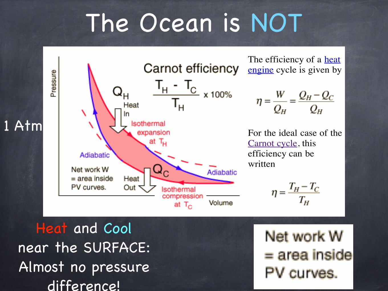
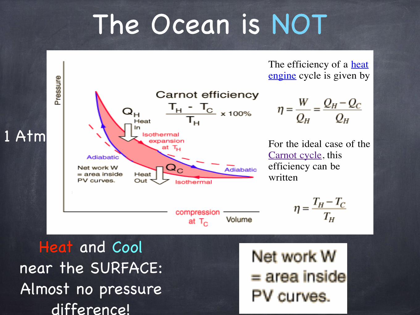
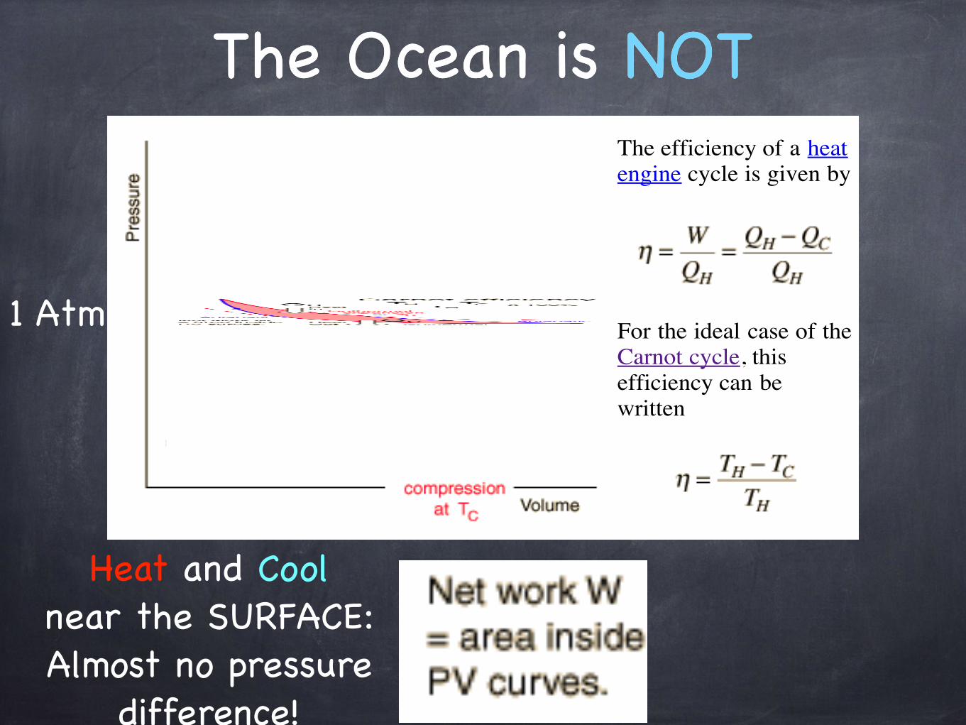
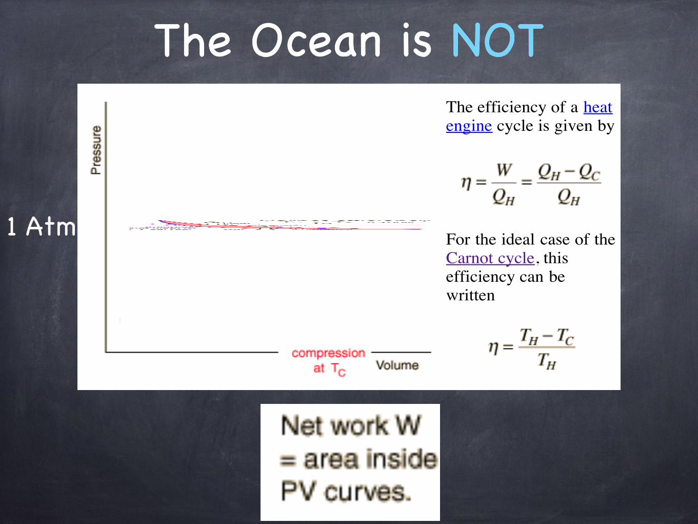
The efficiency of a heatengine cycle is given by

For the ideal case of theCarnot cycle, thisefficiency can bewritten

Using these two expressions together

If we take Q to represent heat added to the system, then heat taken from thesystem will have a negative value. For the Carnot cycle

which can be generalized as an integral around a reversible cycle

Index

Carnotcycle

concepts

Heatengine

concepts

Entropyconcepts

grev ¼R R R

q _QðþÞdV %R R R

q _Qð%ÞdVR R Rq _QðþÞdV

: ð25Þ

Since grev ‡ g, the difference between the two numbersprovides a measure of just how large irreversibilities are.This is discussed in the following section in the contextof the idealized GCM. For this highly simplified GCM,the difference between grev and g is essentially a reflec-tion of energy conservation. However, one could easilyimagine a model in which parameterizations of convec-tion, turbulent diffusion or more complex processes areincluded, whereby the difference between the efficienciesis reflective of irreversibilities due to these parameter-izations.

For a final comparison, the Carnot efficiency for theglobal circulation is calculated. This efficiency is thehighest efficiency possible and, therefore, provides anupper bound on the efficiencies of model-generated cir-culations. It gives a measure of how close to ideal acirculation’s heat engine is. In order to properly calcu-late the Carnot efficiency, it is necessary to weight thetemperature of the heat source and sink by the heatingand cooling rates, respectively. This gives

gc &½Th( % ½Tc(

½Th(; ð26Þ

where [Th] and [Tc] are calculated in the followingmanner:

½Th( ¼1

½ _QðþÞ(

Z Z Z_QðþÞdV

! "; ð27Þ

where ½ _QðþÞ( is the input heating integrated over thevolume. In the case of [Tc], we have

½Tc( ¼1

½ _Qð%Þ(

Z Z Z_Qð%ÞdV

! "; ð28Þ

where ½ _Qð%Þ( is the cooling integrated over the controlvolume. We turn now to applications of these efficienciesto the idealized GCM.

4 Application of framework and discussion

In this section, the sensitivity of the various thermody-namic efficiencies to the modification of physical andnumerical parameters is studied. These experiments aredesigned to provide a ‘‘proof of concept’’ of the idea of

comparing model efficiencies in the assessment of theimportance of irreversibilities. The different experimentscan be classified for convenience into two categories: (1)model numerics and (2) model forcing. For the threeefficiency calculations, steady-state values and at T30resolution were employed. We show below that T30provides sufficient horizontal resolution for these effi-ciency calculations. Specifically, the experiments werestarted from an isothermal state at rest with small per-turbations added to break the symmetry. Integrationswere carried out for 1,000 model days (54,000 time-steps); the model statistics having approached a steady-state (see Figs. 1, 2). The 1,000-day mean, calculatedfrom single daily values, was used to identify the lati-tudinal boundaries of the Hadley cell. The determina-tion of the latitudinal boundaries was based upon thelatitude of maximum vertical velocity and convergenceof the meridional wind. The 1,000-day mean was thenused to restart the experiment. Model integration wasthen carried forward for 1,000 more days in order tocalculate running averages (from all 54,000 timesteps) ofthe necessary quantities for the steady-state energybudget.

4.1 Sensitivity to numerical parameters

Two experiments were carried out in which numericalparameters were modified. These experiments provide asensitivity test of the model’s steady-state solutions tochanges in model numerics. The two experiments in-volved modification of the spectral damping coefficientand changes in the model’s spectral resolution. Resultsare presented for both the general circulation (a closedsystem) and the Hadley cell (an open system).

4.1.1 Spectral damping

The idealized GCM does not have explicit diffusion andonly a scale-selective horizontal mixing is included. Theform of this mixing of vorticity, divergence and tem-perature is a Laplacian raised to the fourth power whosestrength is set to that of an e-folding time of 0.1 days forthe shortest wave. The purpose of this mixing is toprevent the accumulation of energy at the high fre-quencies to control non-linear instabilities. The spectraldamping coefficient was varied by modifying thee-folding time for the smallest wave from between0.2 days; that is, stronger damping, to values of0.005 days; that is, weaker damping. Table 1 summa-rizes the results of these experiments. Reducing thespectral damping results in a more energetic global cir-culation. Frictional dissipation increases by about 30%between the experiments with strong and weak dampingand g, the thermodynamic efficiency based on work,increases. The increase in heat input rate is onlyapproximately 10%, and relative changes in Qnet andQ(+) are small. Hence, the heat-based and Carnot

Table 1 Global thermodynamic efficiencies versus spectral damp-ing coefficient

Efficiency Spectral damping coefficient (day%1)

0.005 0.01 0.05 0.1 0.15 0.2

g 9.12 9.21 8.74 8.17 6.69 7.29grev 12.27 12.47 11.92 12.04 11.77 12.77gc 13.24 13.49 13.34 13.49 13.64 14.64

Adams and Renno: Thermodynamic efficiencies of an idealized global climate model 807

Adams & Renno 2005:

Nave, 2005The atmosphere converts

heating & cooling to kinetic energy that does work.

It’s roughly 10-15% as efficent as ideal thermal engines.

The Ocean is NOT




Nave

Go Back







Index

Carnotcycle

concepts

Heatengine

concepts

Entropyconcepts




Nave

Go Back







Index

Carnotcycle

concepts

Heatengine

concepts

Entropyconcepts




Nave

Go Back







Index

Carnotcycle

concepts

Heatengine

concepts

Entropyconcepts

Heat and Cool near the SURFACE: Almost no pressure

difference!

1 Atm

The Ocean is NOT




Nave

Go Back







Index

Carnotcycle

concepts

Heatengine

concepts

Entropyconcepts




Nave

Go Back







Index

Carnotcycle

concepts

Heatengine

concepts

Entropyconcepts




Nave

Go Back







Index

Carnotcycle

concepts

Heatengine

concepts

Entropyconcepts


difference!

1 Atm

The Ocean is NOT

The Ocean is NOT




Nave

Go Back







Index

Carnotcycle

concepts

Heatengine

concepts

Entropyconcepts




Nave

Go Back







Index

Carnotcycle

concepts

Heatengine

concepts

Entropyconcepts




Nave

Go Back







Index

Carnotcycle

concepts

Heatengine

concepts

EntropyconceptsHeat and Cool

near the SURFACE: Almost no pressure

difference!

1 Atm

The Ocean is NOT

The Ocean is NOT




Nave

Go Back







Index

Carnotcycle

concepts

Heatengine

concepts

Entropyconcepts




Nave

Go Back







Index

Carnotcycle

concepts

Heatengine

concepts

Entropyconcepts




Nave

Go Back







Index

Carnotcycle

concepts

Heatengine

concepts

Entropyconcepts


difference!

1 Atm

The Ocean is NOT

The Ocean is NOT




Nave

Go Back







Index

Carnotcycle

concepts

Heatengine

concepts

Entropyconcepts




Nave

Go Back







Index

Carnotcycle

concepts

Heatengine

concepts

Entropyconcepts




Nave

Go Back







Index

Carnotcycle

concepts

Heatengine

concepts

Entropyconcepts

1 Atm

The Ocean is NOT

Elaborate Schemes: Ocean Transports Heat, But winds drive the system.. plus tides and geothermal...

(Sandstrom 1916, Wunsch & Ferrari 04)

13 Dec 2003 18:52 AR AR203-FL36-12.tex AR203-FL36-12.sgm LaTeX2e(2002/01/18) P1: IBD

302 WUNSCH � FERRARI

Figure 5 Strawman energy budget for the global ocean circulation, with uncertainties of

at least factors of 2 and possibly as large as 10. Top row of boxes represent possible energy

sources. Shaded boxes are the principal energy reservoirs in the ocean, with crude energy

values given [in exajoules (EJ) 1018 J, and yottajoules (YJ) 1024 J]. Fluxes to and from the

reservoirs are in terrawatts (TWs). Tidal input (see Munk & Wunsch 1998) of 3.5 TW is

the only accurate number here. Total wind work is in the middle of the range estimated by

Lueck & Reid (1984); net wind work on the general circulation is from Wunsch (1998).

Heating/cooling/evaporation/precipitation values are all taken from Huang & Wang (2003).

Value for surface waves and turbulence is for surface waves alone, as estimated by Lefevre

& Cotton (2001). The internal wave energy estimate is by Munk (1981); the internal tide

energy estimate is from Kantha & Tierney (1997); the Wunsch (1975) estimate is four times

larger. Oort et al. (1994) estimated the energy of the general circulation. Energy of the

mesoscale is from the Zang &Wunsch (2001) spectrum (X. Zang, personal communication,

2002). Ellipse indicates the conceivable importance of a loss of balance in the geostrophic

mesoscale, resulting in internal waves and mixing, but of unknown importance. Dashed-dot

lines indicate energy returned to the general circulation by mixing, and are first multiplied

by �. Open-ocean mixing by internal waves includes the upper ocean.

such kinetic energy exist, the wind stress and tidal flows. The tides can account

for approximately 1 TW, at most. The wind field provides approximately 1 TW—

directly—to the large-scale circulation and probably at least another 0.5 TW by

generating inertial waves and the internal wave continuum.

Taken together, Sandstrom’s (1908, 1916) and Paparella & Young’s (2002)

theorems, the very small, probably negative, contribution to oceanic potential

energy by buoyancy exchanges with the atmosphere, and the ready availability of

An

nu

. R

ev.

Flu

id.

Mec

h.

20

04

.36

:28

1-3

14

. D

ow

nlo

aded

fro

m a

rjo

urn

als.

ann

ual

rev

iew

s.o

rgb

y M

AS

SA

CH

US

ET

TS

IN

ST

. O

F T

EC

HN

OL

OG

Y o

n 0

3/0

7/0

5.

Fo

r p

erso

nal

use

on

ly.

But Does it matter?A man falls to his death after being pushed from the Empire State Building Observatory. Who is responsible?

Clearly, he was killed by kinetic energy! So, the source of KE is the culprit!

The push was horizontal, thus it supplies no PE and precious little KE.

Most of the KE was converted from PE,

Or, if he took the elevator, then the power company is to blame...

BUT, the company used oil from the Middle East...

The pusher is innocent!

Thus, if he took the stairs, it was suicide

You see how we get in trouble...

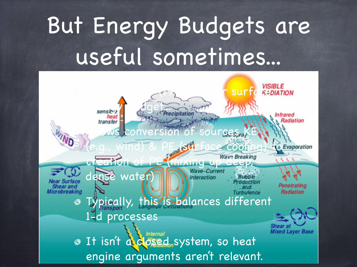
But Energy Budgets are useful sometimes...

Kraus-Turner (1967): near surface energy budget...

Allows conversion of sources KE (e.g., wind) & PE (surface cooling) to creation of PE (mixing up deep, dense water)

Typically, this is balances different 1-d processes

It isn’t a closed system, so heat engine arguments aren’t relevant.

Leads us to thinking about PE:

Potential Energy is just , where z is height and b is buoyancy,

So increase PE by cooling at surface, decrease PE by heating at surface.

In order to move dense water up, you have to input energy (e.g., by mixing with wind or tides)

Instabilities rely on extracting energy. Baroclinic instabilities extract PE by net vertical transport of light water up, cold

⟨−zb⟩

b ≡−g(ρ − ρ0)

ρ0

⟨w′b′⟩ > 0

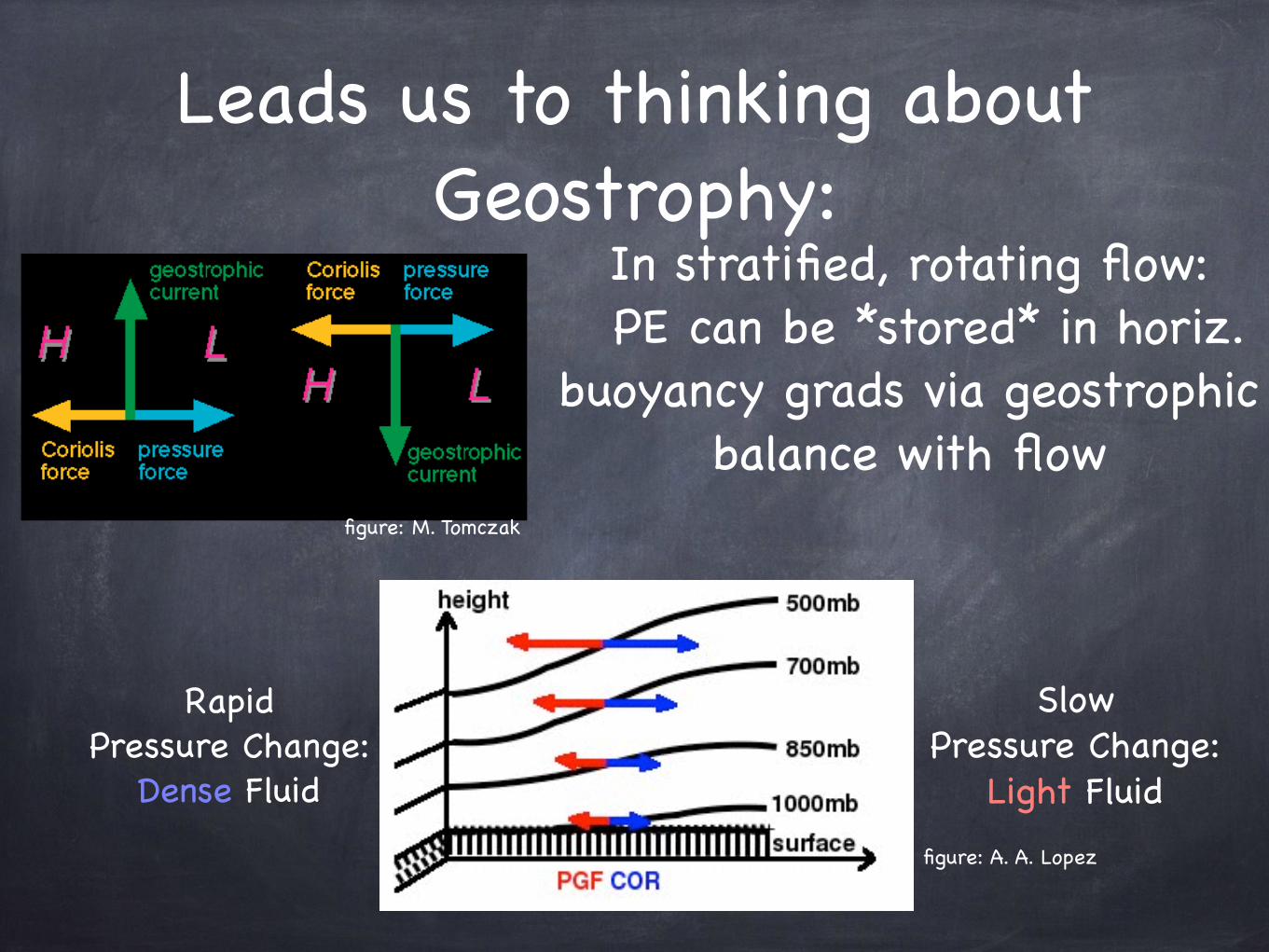
Leads us to thinking about Geostrophy:

figure: M. Tomczak

figure: A. A. Lopez

Rapid Pressure Change:

Dense Fluid

Slow Pressure Change:

Light Fluid

In stratified, rotating flow: PE can be *stored* in horiz. buoyancy grads via geostrophic

balance with flow

Leads us to thinking about Geostrophic ScalesIn stratified, rotating flow:

Stored PE=KE at the scale of the Deformation Radius, or Rossby Radius

This scale is also the width over which an adjusting front slumps,

And sets the typical scale of baroclinic instability eigenvectors

H N/f

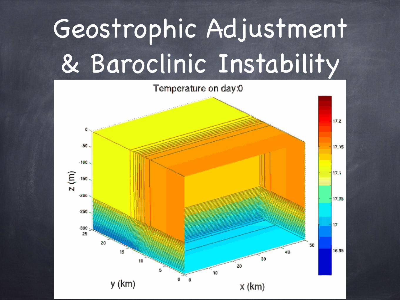
Geostrophic Adjustment & Baroclinic Instability

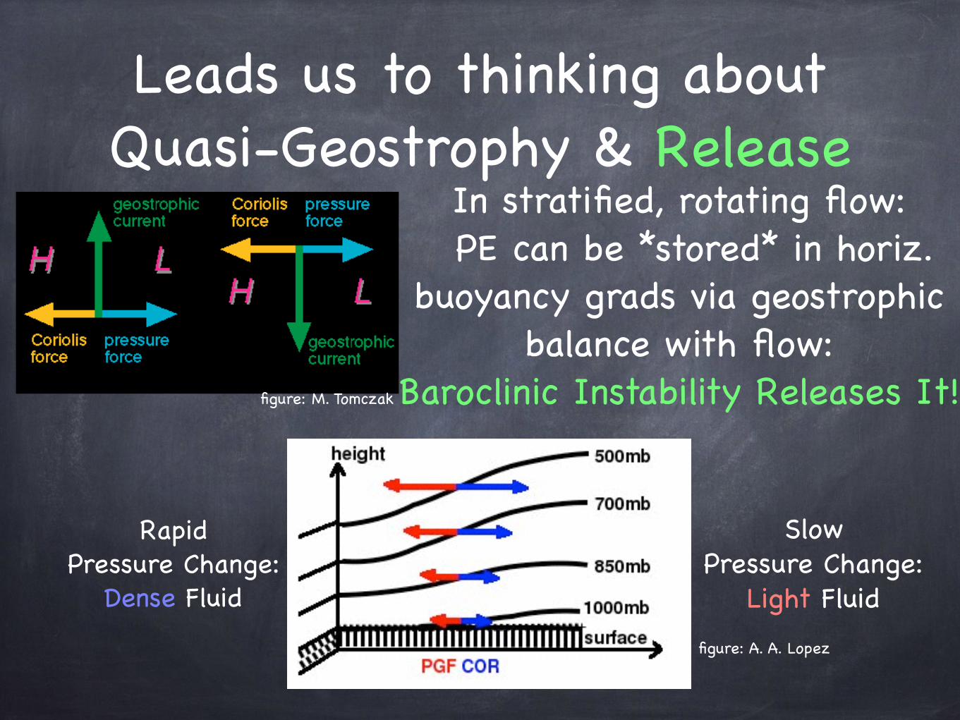
Leads us to thinking about Quasi-Geostrophy & Release

figure: M. Tomczak

figure: A. A. Lopez

Rapid Pressure Change:

Dense Fluid

Slow Pressure Change:

Light Fluid

In stratified, rotating flow: PE can be *stored* in horiz. buoyancy grads via geostrophic

balance with flow: Baroclinic Instability Releases It!

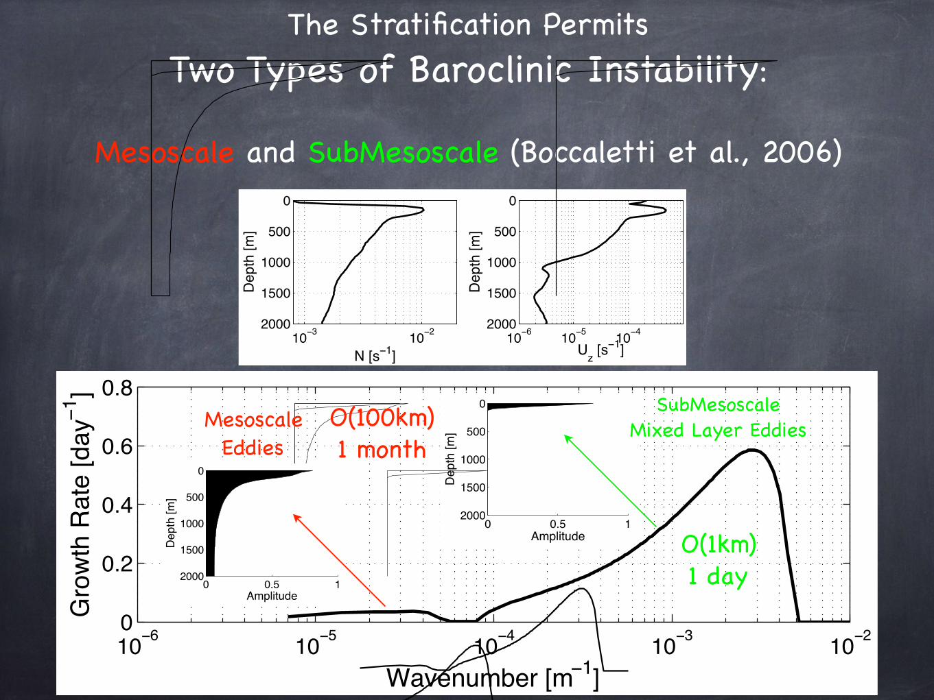
The Stratification Permits Two Types of Baroclinic Instability:

Mesoscale and SubMesoscale (Boccaletti et al., 2006)42

!"!#

!"!$

"

%""

!"""

!%""

$"""

&'()*+,-.

/+,0!!.

!"!1

!"!%

!"!2

"

%""

!"""

!%""

$"""

&'()*+,-.

34+,0!!.

Figure 2: Buoyancy frequency N2 =−g!z/!0 and vertical shearUz = g!x/ f!0 estimated from the133-130◦ W SeaSoar section shown in Fig. 1. The vertical gradients are computed across 8 m,

while the horizontal gradients are computed across 10 km. The profiles are extended to the ocean

bottom by matching the SeaSoar estimates in the upper 320 m with estimates based on Levitus

climatology for the rest of the water column. Details of the calculation are given in Appendix A.

43

! !"# $

!

#!!

$!!!

$#!!

%!!!

&'()*+,-.

/.(+012'3

! !"# $

!

#!!

$!!!

$#!!

%!!!

&'()*+,-.

/.(+012'3

$!!4

$!!#

$!!5

$!!6

$!!%

!

!"%

!"5

!"4

!"7

89:;+01<=+.12-=>!$3

[email protected],'B.912'!$3

Figure 3: Stability analysis of the mean shear shown in Fig. 2.The instability is dominated by

two distinct modes: an interior instability with wavelength close to the internal deformation radius

(approx60 km) and a mixed-layer instability (MLI) peaking at wavelength close to the ML defor-

mation radius (≈ 2 km). The interior instability has a spatial structure (upper left panel) spanningthe whole thermocline depth and represents the mesoscale restratification due to quasigeostrophic

baroclinic instability (Eady, 1949). TheMLI (upper left panel) is confined to the ML and represents

restratification due to ageostrophic instability within the ML (Stone, 1971).

43

! !"# $

!

#!!

$!!!

$#!!

%!!!

&'()*+,-.

/.(+012'3

! !"# $

!

#!!

$!!!

$#!!

%!!!

&'()*+,-.

/.(+012'3

$!!4

$!!#

$!!5

$!!6

$!!%

!

!"%

!"5

!"4

!"7

89:;+01<=+.12-=>!$3








43

! !"# $

!

#!!

$!!!

$#!!

%!!!

&'()*+,-.

/.(+012'3

! !"# $

!

#!!

$!!!

$#!!

%!!!

&'()*+,-.

/.(+012'3

$!!4

$!!#

$!!5

$!!6

$!!%

!

!"%

!"5

!"4

!"7

89:;+01<=+.12-=>!$3








Mesoscale Eddies

SubMesoscale Mixed Layer EddiesO(100km)

1 month

O(1km) 1 day

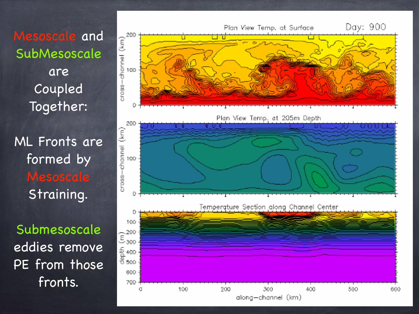
Mesoscale and SubMesoscale

are Coupled Together:

ML Fronts are formed by Mesoscale Straining.

Submesoscale eddies remove PE from those

fronts.

But, Resolving both the Mesoscale and Submesoscale is

expensive

What we need is a Prototypical Problem to

Parameterize!

But, Resolving both the Mesoscale and Submesoscale is

expensive

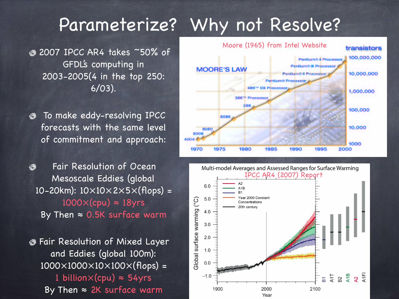
Parameterize? Why not Resolve?2007 IPCC AR4 takes ~50% of

GFDL’s computing in 2003-2005(4 in the top 250:

6/03).

To make eddy-resolving IPCC forecasts with the same level of commitment and approach:

Fair Resolution of Ocean Mesoscale Eddies (global

10-20km): 10×10×2×5×(flops) = 1000×(cpu) ≈ 18yrs

By Then ≈ 0.5K surface warm

Fair Resolution of Mixed Layer and Eddies (global 100m):

1000×1000×10×100×(flops) = 1 billion×(cpu) ≈ 54yrs

By Then ≈ 2K surface warm

Moore (1965) from Intel Website

IPCC AR4 (2007) Report

So, for submesoscale in a climate model:

Not DNS...Not LES...

NES:No Eddy Simulation!

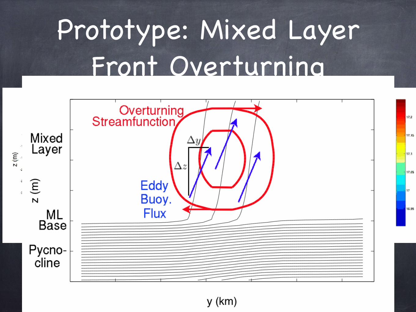
Prototype: Mixed Layer Front Overturning

Simple Spindown Plus, Diurnal Cycle and KPP

Note: initial geostrophic adjustment overwhelmed by eddy restratification

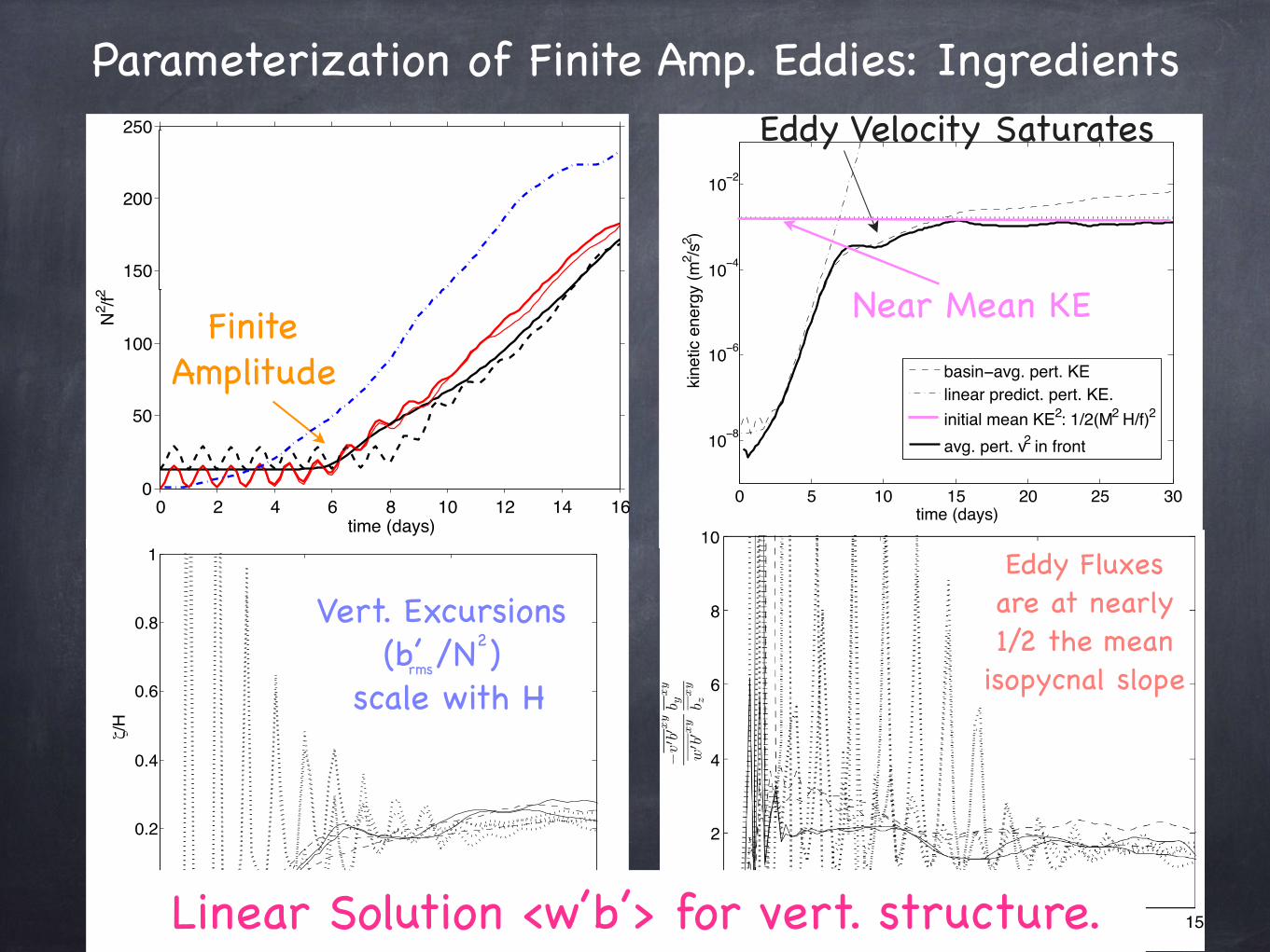
Parameterization of Finite Amp. Eddies: Ingredients

Vert. Excursions (b’ /N )

scale with H

Finite Amplitude

0 5 10 150

0.2

0.4

0.6

0.8

1

time (days)

!/H

0 5 10 15 20 25 30

10!8

10!6

10!4

10!2

time (days)

kin

etic e

nerg

y (

m2/s

2)

basin!avg. pert. KE

linear predict. pert. KE.

initial mean KE2: 1/2(M

2 H/f)

2

avg. pert. v2 in front

Eddy Velocity Saturates

Near Mean KE

rms

2

0 2 4 6 8 10 12 14 160

50

100

150

200

250N

2/f

2

time (days)

unbalanced, Ri0=0

unbalanced, Ri0=1

balanced, Ri0=1

hi−res unbal, Ri0=0

bal, Ri0=0

Eddy Fluxes are at nearly 1/2 the mean

isopycnal slope

Linear Solution <w’b’> for vert. structure.

Magnitude Analysis: Vert. Fluxes

∆z ∝ H

∆y

∆z∝

−∂b∂z

∂b∂y

≈∆PE

∆t∝

∆z∆b

∆t

⟨wb⟩ ∝H2

|f |

!

∂b

∂y

"2

−⟨wb⟩ =

∂⟨PE⟩

∂t

Extraction of potential energy by submesoscale eddies:

Buoy. diff just parcel exchange of large-scale buoy.

Flux slope scales with the buoy. slope:

Vertical scale known:

Time scale is turnover time

⟨wb⟩ ∝∆z∆y ∂b

∂y

∆t⟨wb⟩ ∝

∆z∆y ∂b∂y

∆y/V⟨wb⟩ ∝

∆zH

|f |

!

∂b

∂y

"2

from mean thermal wind:

⟨wb⟩ ∝−∆z∆b

∆t⟨wb⟩ ∝

−∆z!

∆y ∂b∂y

+ ∆z ∂b∂z

"

∆t Fox-Kemper et al., 2007

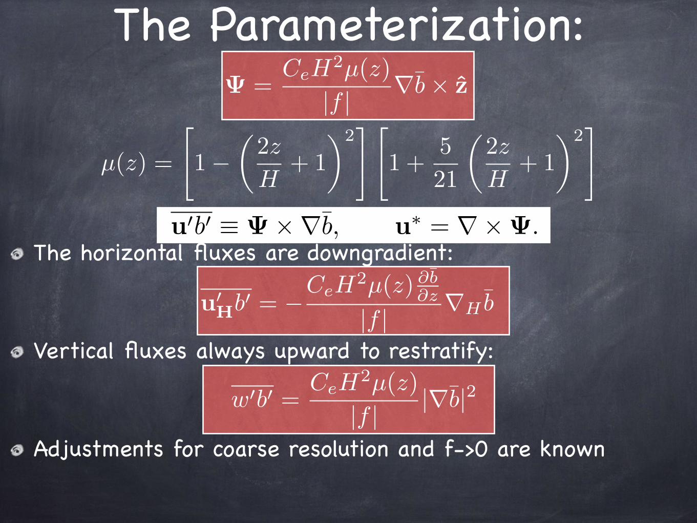
The Parameterization:Ψ =

CeH2µ(z)

|f |∇b × z

w′b′ =CeH

2µ(z)

|f ||∇b|2

u′

Hb′ = −

CeH2µ(z) ∂b

∂z

|f |∇H b

µ(z) =

!

1 −

"

2z

H+ 1

#2$ !

1 +5

21

"

2z

H+ 1

#2$

The horizontal fluxes are downgradient:

Vertical fluxes always upward to restratify:

Adjustments for coarse resolution and f->0 are known

30 March 2007 FOX-KEMPER, FERRARI, and HALLBERG 15

that this scatter is associated with erroneous depen-dence on the time-evolving Ri, rather than otherfactors. (Using the initial value of Ri produces anorder of magnitude more scatter for these scalings,not shown). Fig. 14e shows there is no systematictrend with Ri in the departures of ⇤d from (20),nor is there a systematic trend with the initial valueof Ri (not shown). Dependence on Ro through Lf ,as in (29) and as assumed by Haine and Marshall(1998) is irrelevant as soon as �y > Lf , which oc-curs soon after finite amplitude is attained. A figurelike Fig. 14e, but with Ro as ordinate shows no de-pendence on Ro (not shown).

Additional potentially relevant nondimensionalquantities might appear, such as (H/Lf ), Smagorin-sky coe�cient (Sm), grid resolution to frontwidth (�x/Lf ), diurnal cycle timescale to inertialtimescale f/⌅, and interior stratification to MLstratification (Nml/Nint). Nonlinear optimizationwas used to test sets of nondimensional parameters(Pi) to find exponents b(i) and the e�ciency factorCe that reduced the di⇧erence between ⇤d and theproduct of parameters, CeH2M2|f |�1⇥iP

b(i)i . By

this method, an Ekman number, Ek ⇤ ⇥H�2f�1,factor of approximately Ek�0.2 was found to im-prove the results. No robust dependence on anyother nondimensional parameter was found (i.e.,,the exponents were less than 0.1 in magnitude).Haine and Marshall (1998) note that the parame-ter space needed to distinguish potential scalings isoften unexplored. Even the 241 simulations hereneglect some part of parameter space. Neglected re-gions include nonhydrostatic e⇧ects (H/Lf = O(1)),barotropic instabilities of the front (RiRo2 ⌅ 1),and viscosity su�cient to stabilize the ML instabil-ities. However, the scaling presented here spans theregime relevant for MLEs.

5. Summary and Conclusion

Observations and numerical simulations reveal thatthe ML is host to shallow frontal instabilities thatact to restratify the ML. This paper presents a pa-rameterization of the restratification by these in-stabilities cast as a streamfunction to represent theoverturning of the front. The parameterization de-pends on the horizontal buoyancy gradients and pro-vides a first attempt at incorporating the interac-tion of lateral gradients and vertical mixing in theML. This parameterization will provide GCMs witha novel climate sensitivity, so far ignored by otherML parameterizations. In three dimensions, the pa-

rameterization takes the form,

� = CeH2⌃b

z⇥z|f | µ(z), (38)

µ(z) =⇤1�

�2zH + 1

⇥2⌅ ⇤

1 + 521

�2zH + 1

⇥2⌅, (39)

u⌅b⌅ ⇤ �⇥⌃b, u⇤ = ⌃⇥�. (40)

with Ce between 0.06 and 0.08. Two companion pa-pers (Fox-Kemper and Ferrari, 2007; Fox-Kemperet al., 2007) give further insight into the skill, im-plementation, and importance for climate of the pa-rameterization.

Previous attempts to include eddy driven restrat-ification by horizontal buoyancy gradients in MLmodels relied on ad hoc modification of the GMmesoscale eddy parameterization through taperingfunctions. This approach fails as the mesoscale hor-izontal fluxes–were they to flux along the shallowML slopes–imply excessive vertical fluxes and re-stratify the ML immediately. Indeed, the GM ta-pering schemes are introduced precisely to avoid in-stantaneous ML restratification. In contrast, MLEsprovide the correct amount of eddy restratificationfor the ML.

The approach in developing this parameterizationis novel in that scaling arguments are derived di-rectly for the overturning streamfunction instead ofrelying on di⇧usive closures for the horizontal eddyfluxes. The scaling simply constrains the stream-function to release PE at the rate expected for baro-clinic spindown. Working in terms of di⇧usivities of-fers less obvious constraints. Furthermore, the pa-rameterization avoids parameters that are di�cultin modeling practice: Ri, deformation radius, in-stability length scale, or the width of a ’barocliniczone’. Only the readily available ML depth and hor-izontal buoyancy gradient are needed. (The issue ofestimating the relevant horizontal buoyancy gradi-ent in a coarse model is discussed in Fox-Kemperet al. (2007).) In principle, the approach here couldbe extended to a mesoscale parameterization for usein the ocean interior, but the nontrivial complica-tions of variable background stratification are leftfor a future investigation.

A few observational studies prove the existenceand ubiquity of MLEs. Flament et al. (1985) observethe development of small-scale eddies along a MLfront that compare favorably with the phenomenahere. Munk et al. (2000) have noted MLEs in photostaken by Astronaut Scully-Power. Recent observa-tions also suggest the tendency for MLEs to releasePE from fronts (D’Asaro, pers. comm.). Houghtonet al. (2006) detect submesoscale along-isopycnal fil-

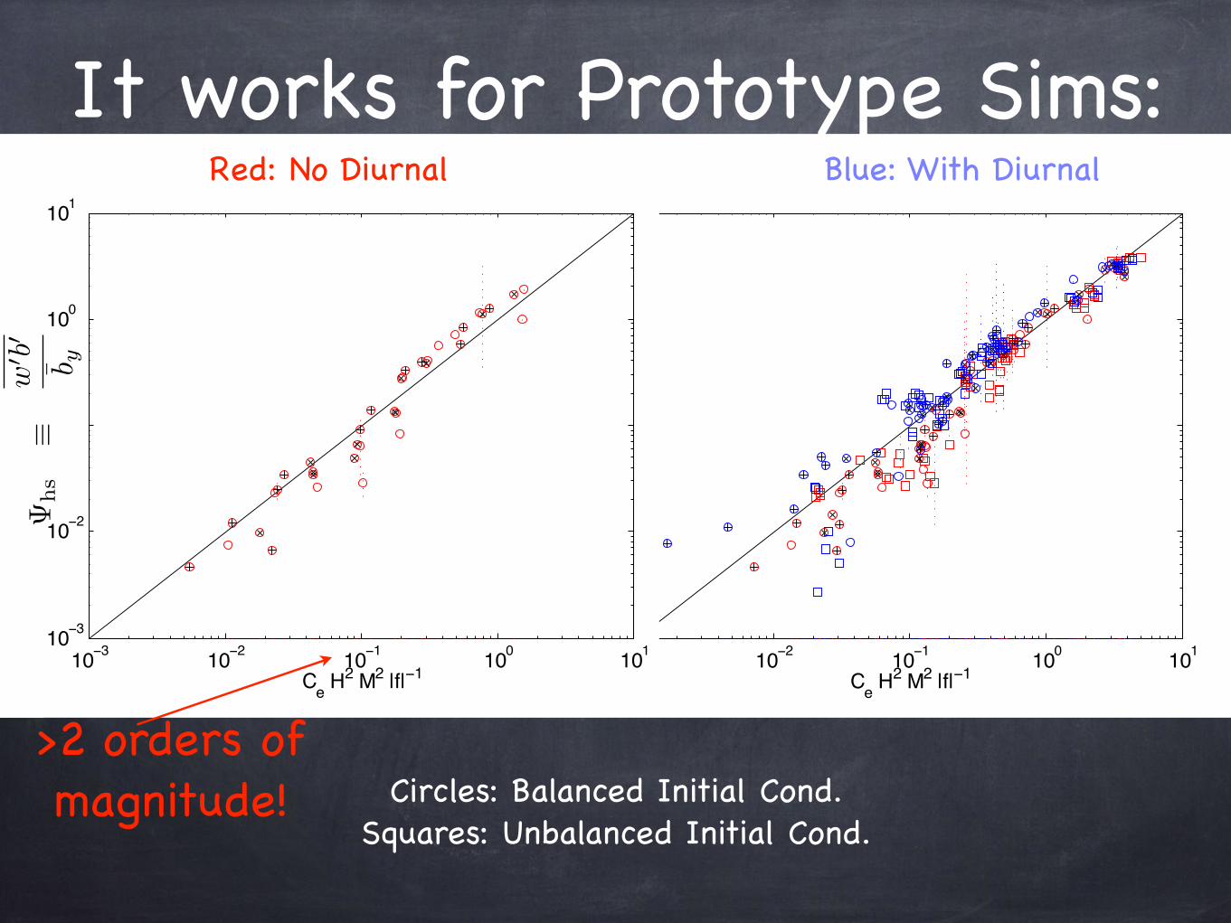
It works for Prototype Sims:

Circles: Balanced Initial Cond. Squares: Unbalanced Initial Cond.

>2 orders of magnitude!

Red: No Diurnal Blue: With Diurnal

10!3

10!2

10!1

100

101

10!3

10!2

10!1

100

101

Ce H

2 M

2 |f|!1

!d

10!3

10!2

10!1

100

101

10!3

10!2

10!1

100

101

Ce H

2 M

2 |f|!1

!d

29Ja

nuar

y20

07FO

X-K

EM

PER

,FER

RA

RI,

and

HA

LLB

ER

G7

boun

dary

-nor

mal

velo

citi

esva

nish

.

�b

�t

+⌅

·ub+⌅

·u� b

�=

D,

(6)

dPE

dt=

d dt�

zbxyz

=�

wbx

yz.

(7)

a.M

agni

tude

ofth

eO

vert

urni

ng

The

first

step

info

rmin

gth

epa

ram

eter

izat

ion

isde

-te

rmin

ing

the

mag

nitu

desc

alin

gof

the

vert

ical

and

hori

zont

aled

dybu

oyan

cyflu

xes.

MLE

sre

sult

from

baro

clin

icin

stab

ility

,whi

chre

-le

ases

PE

from

the

mea

nflo

w.

Con

side

rth

eP

Eex

trac

tion

byex

chan

geof

fluid

parc

els

over

deco

r-re

lation

dist

ance

s�

yan

d�

zin

ati

me

�t.

�P

E�

t⇤

��

z� �

yM2

+�

zN2⇥

�t

,

We

may

estim

ate

the

extr

acti

onra

teby

assu

min

g

1.T

here

leva

ntti

mes

cale

�t

isth

eti

me

itta

kes

for

aned

dyto

trav

erse

the

deco

rrel

atio

nle

ngth

(�t⇤

|�y/

U|=

|�z/

W|).

2.T

heho

rizo

ntal

eddy

velo

city

scal

esas

the

mea

nth

erm

alw

ind

U⇤

⇤ ⇤ M2H

/f⇤ ⇤ (

see

Fig

.5).

3.T

heve

rtic

alde

corr

elat

ion

leng

thsc

ales

wit

hth

eM

Lde

pth

�z⇤

H(s

eeFig

.6).

4.Flu

idex

chan

geoc

curs

alon

ga

slop

ebe

low

(i.e

.,P

Eex

trac

ting

)an

dpr

opor

tion

alto

the

mea

nis

opyc

nals

lope

(⇤ ⇤ �yM

2⇤ ⇤ =

C�

zN2

whe

reC

>1,

see

Fig

.7).

Thu

s,

�P

E�

t⇤

�C

+1

C

M4H

2

|f|

.(8

)

The

MLE

flux

scal

ings

may

befo

und

byno

ting

that

our

sim

ulat

ions

,th

eM

LEve

rtic

alflu

xdo

mi-

nate

sth

em

ean

in(7

).T

hus,

w� b

�xyz⇤

C�

1C

M4H

2

|f|

.(9

)

Ass

umpt

ion

4al

soim

plie

s

v�b�

xyz

=�

Cw

� b�x

yzN

2

M2

⇤�

(C�

1)M

2N

2H

2

|f|

.(10

)

Soas

inFig

.8,th

eve

rtic

alflu

xis

upw

ard

and

v�b�

isdo

wn

the

mea

nbu

oyan

cygr

adie

nt.

b.The

Ove

rtur

ning

Stre

amfu

nction

Apa

ram

eter

izat

ion

coul

dbe

mad

edi

rect

lyfr

om(1

0)an

d(9

),bu

tin

trod

uction

ofan

over

turn

ing

stre

amfu

nction

aids

impl

emen

tation

ina

num

eric

alm

odel

.T

heed

dybu

oyan

cyflu

xes

may

bebr

oken

into

ask

ewflu

xge

nera

ted

bya

stre

amfu

ncti

on(v

� sb�⇥

�⇥

b z,w

� sb�⇥

⇥b y

)an

dth

ere

mai

ning

residu

alflu

x.U

sing

ast

ream

func

tion

in(6

)yi

elds

,

⌅·u

� b�

=�

� �y

� ⇥b z

⇥ +� �z

� ⇥b y

⇥(1

1)

+�(v

� b��

v� sb�

)�y

+�(w

� b��

w� sb�

)�z

,

Ifth

ere

sidu

alflu

xesw

ere

tova

nish

,the

nth

est

ream

-fu

ncti

onw

ould

beun

ique

and

wou

ldge

nera

teal

lof

the

eddy

fluxe

s.H

owev

er,

inth

ese

sim

ulat

ions

,th

ere

sidu

alflu

xdo

esno

tva

nish

.Tra

dition

ally

,the

stre

amfu

nction

isch

osen

toel

imin

ate

the

hori

zont

alre

sidu

alflu

x(A

ndre

ws

and

McI

ntyr

e,19

78;P

lum

ban

dFe

rrar

i,20

05),

⇥tr

⇥�

v�b�

b z,

(12)

⌅·u

� b�

=�

� �y

� ⇥tr

b z⇥ +

� �z

� ⇥tr

b y⇥

(13)

+�(w

� b��

w� sb�

)�z

.

How

ever

,in

(13)

both

the

skew

and

resi

dual

fluxe

sw

ould

need

tobe

para

met

eriz

edan

dst

ably

pro-

duce

the

upgr

adie

nt,

antidi

⇤usi

veto

tal

flux

in(9

):a

daun

ting

num

eric

alta

sk.

The

Hel

dan

dSc

hnei

der

(199

9)st

ream

func

tion

,⇥hs,

ism

ore

conv

enie

nt.

⇥hs⇥

w� b

�

b y,

(14)

⌅·u

� b�

=�

� �y

� ⇥hsb

z

⇥ +� �z

� ⇥hsb

y

⇥(1

5)

+�(v

� b��

v� sb�

)�y

.

Thi

sch

oice

hasad

vant

ages

inth

eM

Lse

ttin

g.Fir

st,

⇥hs

allo

ws

easy

impl

emen

tation

of(9

).Se

cond

,⇥hs

vani

shes

atth

esu

rfac

eof

the

ocea

nw

itho

utta

per-

ing

asw

� b�

vani

shes

ther

e.T

hird

,⇥

hs

leav

esth

ere

sidu

alflu

xas

ato

tally

hori

zont

al,

and

typi

cally

dow

ngra

dien

tpr

oces

s(i.e

.,whe

nC

>1)

.H

oriz

on-

talfl

uxes

are

dom

inat

edby

the

mea

nan

dm

esos

cale

fluxe

sin

any

case

,th

usth

eho

rizo

ntal

resi

dual

flux

ofte

nm

aybe

safe

lyne

glec

ted

(see

sect

ion

3ean

d?)

.

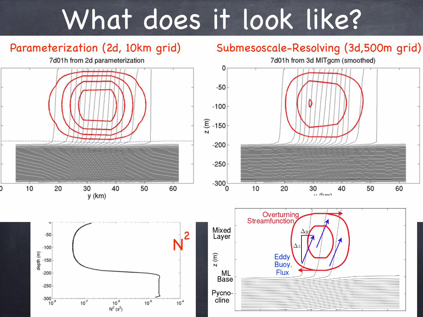
What does it look like?Parameterization (2d, 10km grid) Submesoscale-Resolving (3d,500m grid)

N2

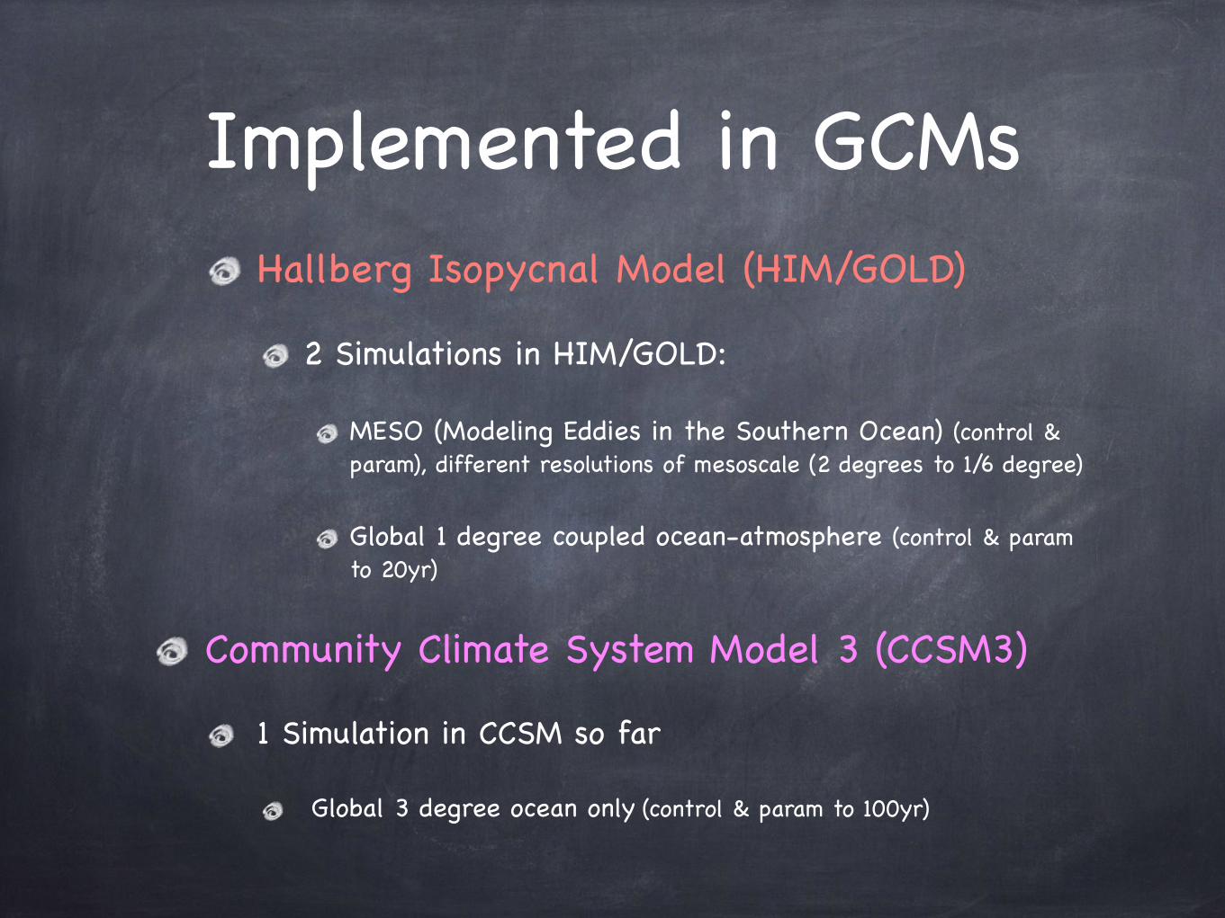
Implemented in GCMs Hallberg Isopycnal Model (HIM/GOLD)

2 Simulations in HIM/GOLD:

MESO (Modeling Eddies in the Southern Ocean) (control & param), different resolutions of mesoscale (2 degrees to 1/6 degree)

Global 1 degree coupled ocean-atmosphere (control & param to 20yr)

Community Climate System Model 3 (CCSM3)

1 Simulation in CCSM so far

Global 3 degree ocean only (control & param to 100yr)

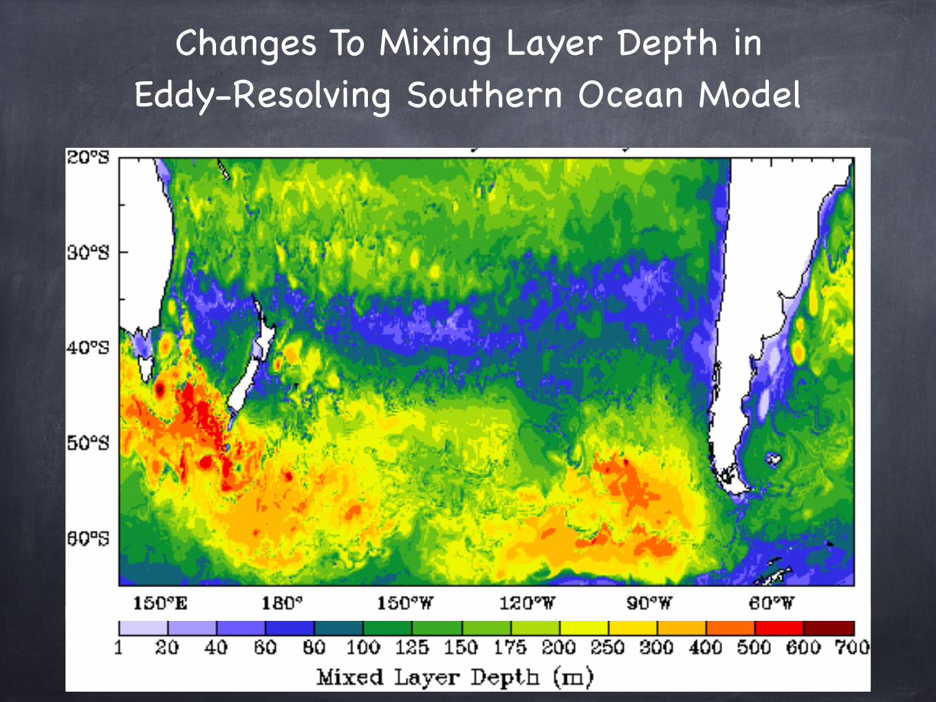
Changes To Mixing Layer Depth in Eddy-Resolving Southern Ocean ModelBulk Mixed Layer New Mixed Layer Model

Bulk Mixed Layer New Mixed Layer Model

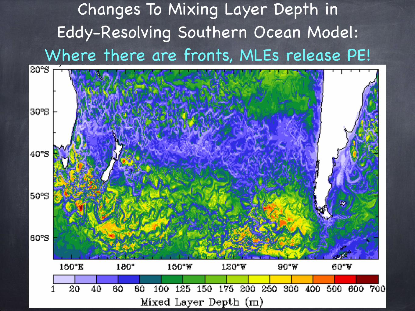
Changes To Mixing Layer Depth in Eddy-Resolving Southern Ocean Model:

Where there are fronts, MLEs release PE!

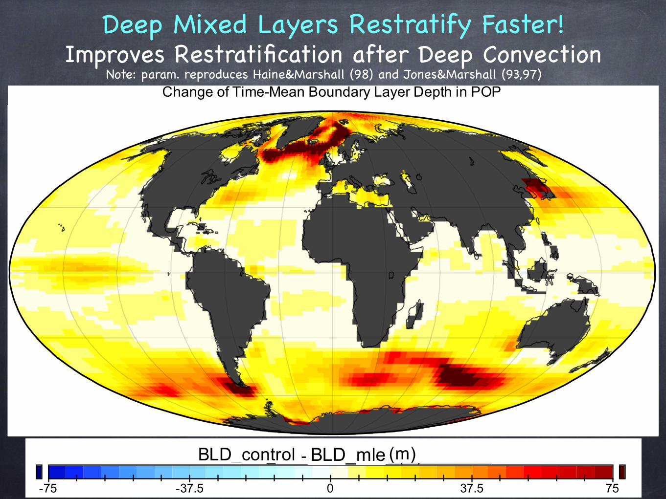
Improves Restratification after Deep ConvectionNote: param. reproduces Haine&Marshall (98) and Jones&Marshall (93,97)

Deep Mixed Layers Restratify Faster!

Data Min = -0.40472, Max = 177.69325Mollweide projection centered on 0.0°E

BLD_mle-BLD_control (m)

-75 -37.5 0 37.5 75

Change of Time-Mean Boundary Layer Depth in POP



-75 -37.5 0 37.5 75

Change of Time-Mean Boundary Layer Depth in GOLD



-75 -37.5 0 37.5 75




-75 -37.5 0 37.5 75




-75 -37.5 0 37.5 75




-75 -37.5 0 37.5 75


Bias Reduction: POP Model Mixed Layer Depth

versus Observations

RMS error: 16m

reduced to 8m

Skewness: 2.4

reduced to 0.6

Submesoscale Conclusion:Submesoscale features, and mixed layer eddies in particular, exhibit large vertical fluxes of buoyancy that are presently ignored in climate models.

A parameterization of mixed layer eddy fluxes as an overturning streamfunction is proposed. The magnitude comes from extraction of potential energy, and the vertical structure resembles the linear Eady solution.

Many observations are consistent, and model biases are reduced. Biogeochemical effects are likely, as vertical fluxes and mixed layer depth are changed.

In HIM and CCSM/POP, soon to be in MITgcm & MOM.

3 Papers so far... Just ask me for them.

Mixing it up! Diagnosing Buoyancy Fluxes & Stirring

Once the potential energy is extracted, the kinetic energy of the mesoscale and submesoscale eddies can be used to stir tracers.

This is an important part of the global tracer transport, and thus of heat, freshwater, pollutants, and greenhouse-gas absorption and storage in the ocean

However, in models with biogeochemistry, we trade high-resolution for reactions, so we have to parameterize all the eddy stirring by NES!

Typically, the parameterizations are ‘trained’ on buoyancy fluxes, but...

One version: Streamfunction

⎡

⎣

u′b′

v′b′

w′b′

⎤

⎦ =

⎡

⎣

0 −Ψz Ψy

Ψz 0 −Ψx

−Ψy Ψx 0

⎤

⎦

⎡

⎣

bx

by

bz

⎤

⎦

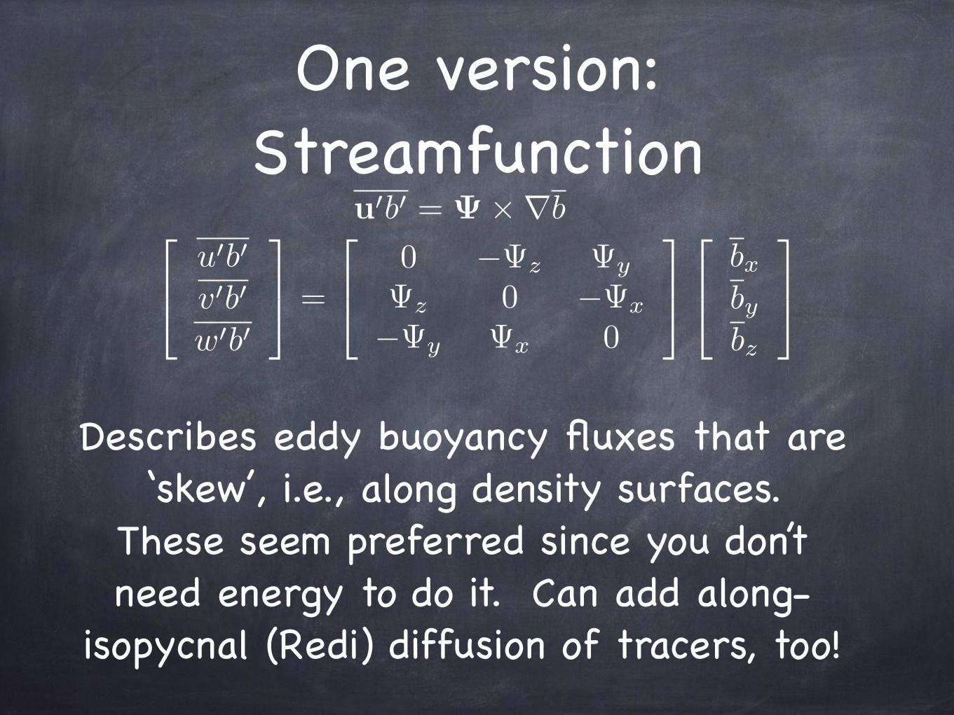
u′b′ = Ψ ×∇b

Describes eddy buoyancy fluxes that are ‘skew’, i.e., along density surfaces.

These seem preferred since you don’t need energy to do it. Can add along-

isopycnal (Redi) diffusion of tracers, too!

One version: Streamfunction

⎡

⎣

u′b′

v′b′

w′b′

⎤

⎦ =

⎡

⎣

0 −Ψz Ψy

Ψz 0 −Ψx

−Ψy Ψx 0

⎤

⎦

⎡

⎣

bx

by

bz

⎤

⎦

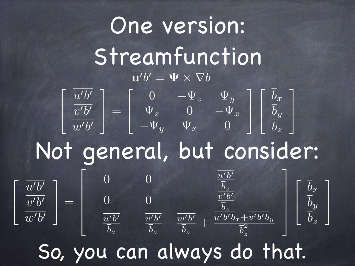
Not general, but consider:

u′b′ = Ψ ×∇b

⎡

⎣

u′b′

v′b′

w′b′

⎤

⎦ =

⎡

⎢

⎢

⎢

⎣

0 0 u′b′

bz

0 0 v′b′

bz

−

u′b′

bz

−

v′b′

bz

w′b′

bz

+u′b′bx+v′b′by

b2

z

⎤

⎥

⎥

⎥

⎦

⎡

⎣

bx

by

bz

⎤

⎦

So, you can always do that.

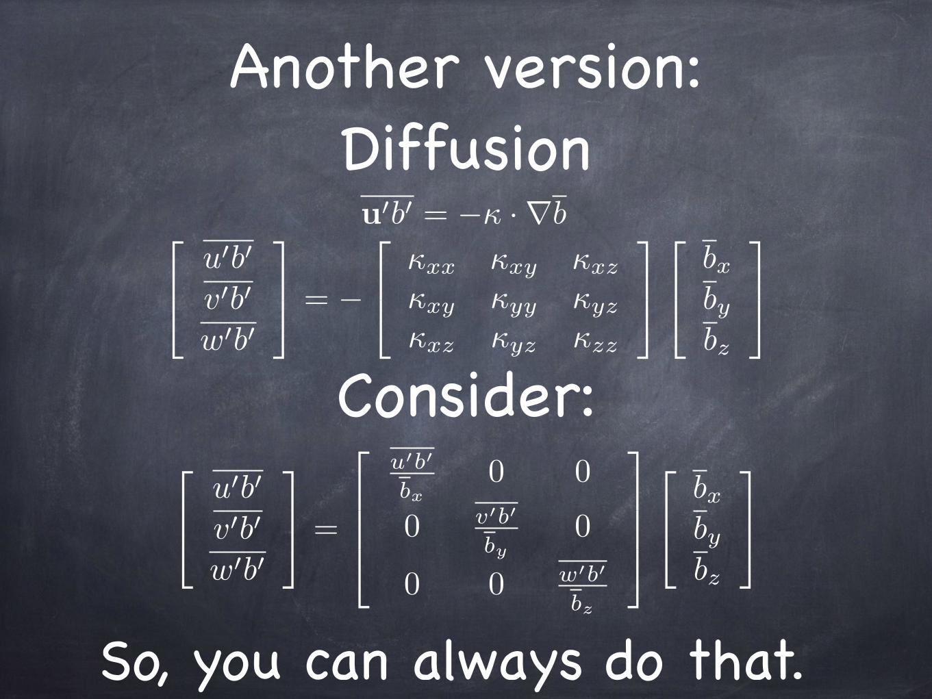
Another version: Diffusion

Consider:

So, you can always do that.

⎡

⎣

u′b′

v′b′

w′b′

⎤

⎦ =

⎡

⎢

⎢

⎣

u′b′

bx

0 0

0v′b′

by

0

0 0w′b′

bz

⎤

⎥

⎥

⎦

⎡

⎣

bx

by

bz

⎤

⎦

⎡

⎣

u′b′

v′b′

w′b′

⎤

⎦

= −

⎡

⎣

κxx κxy κxz

κxy κyy κyz

κxz κyz κzz

⎤

⎦

⎡

⎣

bx

by

bz

⎤

⎦

u′b′ = −κ ·∇b

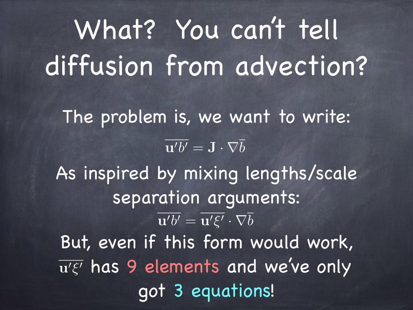
What? You can’t tell diffusion from advection?

The problem is, we want to write:

u′b′ = u

′ξ′ ·∇b

As inspired by mixing lengths/scale separation arguments:

But, even if this form would work, has 9 elements and we’ve only

got 3 equations!u′ξ′

u′b′ = J ·∇b

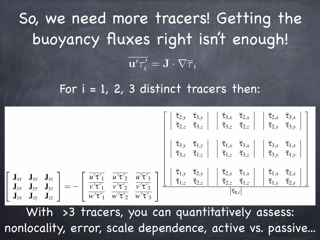
So, we need more tracers! Getting the buoyancy fluxes right isn’t enough!

passive tracers. The method used here initializing and keeping these passive tracers distinct is toinitialize the passive tracer gradients orthogonally, and then weakly restore to the initial, orthogonalconfiguration. Plumb and Mahlman (1987) proved this approach in the GFDL atmospheric model.

3.1 2 Tracers in 2dIn the atmospheric case studied by Plumb and Mahlman (1987) and Bratseth (1998), the averagingoperator is a zonal mean. The stirring tensor J is 2d and has four components: only two tracers arerequired. We can write this out component by component as a matrix equation:

⇥v´⇥´1 v´⇥´2w´⇥´1 w´⇥´2

⇤=�

⇥Jyy JyzJzy Jzz

⇤⇥⇥1,y ⇥2,y⇥1,z ⇥2,z

⇤. (9)

So, if we take the inverse of the tracer gradient matrix (which requires the tracer gradients to beorthogonal, or equivalently for the determinant to be nonzero), then

⇥Jyy JyzJzy Jzz

⇤=�

⇥v´⇥´1 v´⇥´2w´⇥´1 w´⇥´2

⇤1��

⇥1,y ⇥2,y⇥1,z ⇥2,z

��

⇥⇥2,z �⇥2,y�⇥1,z ⇥1,y

⇤. (10)

In the case where the tracer gradients are aligned, then the determinant in the denominator vanishes,and the inversion is not unique. In this case, the stirring matrix is underdetermined, just as in thecase with only one tracer.

3.2 3 tracers in 3dIn three dimensions, the equation is the same in principle but a little uglier, but it is still possible towrite explicitly. In matrix form,

⌅

⌃Jxx Jxy JxzJyx Jyy JyzJzx Jzy Jzz

⇧

⌥=�

⌅

⌃u´⇥´1 u´⇥´2 u´⇥´3v´⇥´1 v´⇥´2 v´⇥´3w´⇥´1 w´⇥´2 w´⇥´3

⇧

⌥

⌅

��⌃

��⇥2,y ⇥3,y⇥2,z ⇥3,z

��

��⇥3,x ⇥2,x⇥3,z ⇥2,z

��

��⇥2,x ⇥3,x⇥2,y ⇥3,y

��

��⇥3,y ⇥1,y⇥3,z ⇥1,z

��

��⇥1,x ⇥3,x⇥1,z ⇥3,z

��

��⇥3,x ⇥1,x⇥3,y ⇥1,y

��

��⇥1,y ⇥2,y⇥1,z ⇥2,z

��

��⇥2,x ⇥1,x⇥2,z ⇥1,z

��

��⇥1,x ⇥2,x⇥1,y ⇥2,y

��

⇧

⌥

|⇥�,i|

Now the determinant of the whole 3d tracer gradient, |⇥�,i|, is required to be nonzero, which requiresthree misaligned gradients.

To verify that the passive tracer restoring approach of Plumb and Mahlman (1987) is valid inthe 3d ocean case, we have completed a short tracer experiment using a 0.4⇥ version of POP as afeasibility test. Three tracers were included, initialized and dampened back towards distributionsproportional to latitude, sine of longitude, and depth respectively. Damping of the first two was ona timescale of 180 days, while that for the last was 10 days at the surface, increasing to 180 days

C–10

u′τ′

i= J ·∇τ i

For i = 1, 2, 3 distinct tracers then:

With >3 tracers, you can quantitatively assess: nonlocality, error, scale dependence, active vs. passive...

Progress on J Tensor Diagnosis (ongoing)

With John Dennis & Frank Bryan (NCAR), and help from LANL (Maltrud) and others (McClean), we’re running a 0.1 degree global ocean model with a suite > 10 tracers at BG/Watson

We’ll see what we see!

Help in thinking about the problem would be appreciated! Difficulties in gauge invariance, etc., need to be sorted before analysis can be completed.

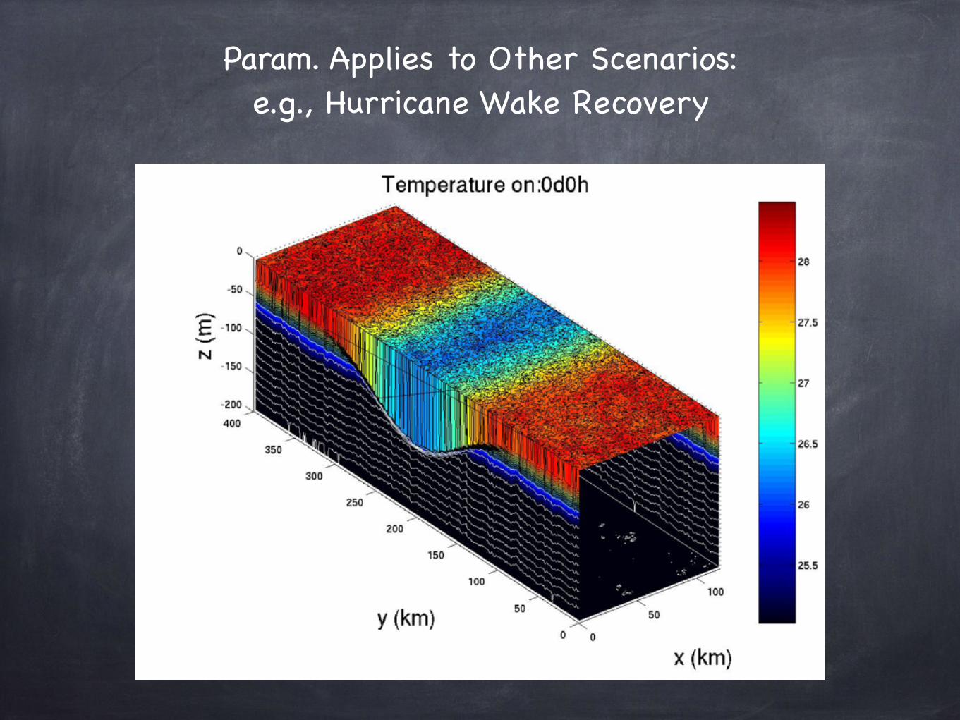
Param. Applies to Other Scenarios: e.g., Hurricane Wake Recovery

Baylor Fox-Kemper - Brown Fluxes in the Ocean... Baylor Fox-Kemper! University of Colorado at...

Documents

Transcript of Baylor Fox-Kemper - Brown Fluxes in the Ocean... Baylor Fox-Kemper! University of Colorado at...