Bayesian Statistics in Software Engineering:Practical Guide and Case Studies

Carlo A. FuriaChalmers University of Technology, Gothenburg, Sweden

furia@chalmers.se bugcounting.net

Abstract—Statistics comes in two main flavors: frequentistand Bayesian. For historical and technical reasons, frequentiststatistics has dominated data analysis in the past; but Bayesianstatistics is making a comeback at the forefront of science. Inthis paper, we give a practical overview of Bayesian statisticsand illustrate its main advantages over frequentist statistics forthe kinds of analyses that are common in empirical softwareengineering, where frequentist statistics still is standard. Wealso apply Bayesian statistics to empirical data from previousresearch investigating agile vs. structured development processes,the performance of programming languages, and random testingof object-oriented programs. In addition to being case studiesdemonstrating how Bayesian analysis can be applied in prac-tice, they provide insights beyond the results in the originalpublications (which used frequentist statistics), thus showing thepractical value brought by Bayesian statistics.

I. INTRODUCTION

A towering figure in evolutionary biology and statistics,Ronald Fisher has exerted a tremendous influence on prettymuch all of experimental science since the early 20th century.The statistical techniques he developed or perfected constitutethe customary data analysis toolset of frequentist statistics,in direct contrast to the other school of statistics—knownas Bayesian since it is ultimately based on Bayes theoremof conditional probabilities. The overwhelming prevalence offrequentist statistics in all the sciences was due partly toFisher’s standing and keen efforts of promotion, partly to itsclaim of being “more objective”, and partly to its techniquesbeing less computationally demanding than Bayesian ones—a crucial concern with the limited computational resourcesavailable in the first part of the past century.

In the last couple of decades, however, the scientific com-munity has begun a critical re-examination of the toolset offrequentist statistics, with particular focus on the widespreadtechnique of statistical hypothesis testing using p-values. Thecritics, who include prominent statisticians such as Cohen [16],have observed methodological shortcomings [17], [31] and,more generally, limitations of the frequentist’s rigid view. Onthe other hand, the difficulties of applying Bayesian analysisdue to its higher computational demands have become mootwith the vast computing power available nowadays. As aresult, Bayesian techniques are becoming increasingly popular,and have buttressed spectacular advances in automation andmachine learning such as the deep neural networks thatpowered Google’s AlphaGo [24].

As we argue in Sect. II, frequentist statistics is still dom-inant in empirical software engineering research, whose bestpractices have been perfected later than in other experimentalsciences. The main contribution of this paper is thus castingthe usage of Bayesian statistics as an alternative and as asupplement to frequentist statistics in the context of the dataanalyses that are common in software engineering.

To make the presentation self contained, in Sect. III webriefly recall some fundamental notions of probability, andthen introduce Bayes theorem—the cornerstone of Bayesiananalysis. In Sect. III-B we explain the shortcomings offrequentist statistical hypothesis testing, and suggest Bayesfactors as an alternative technique. We also present otheranalyses that are fueled by Bayes theorem, and argue aboutthe significant advantages of taking a Bayesian point of view.

In Sect. IV we then proceed to “eat our own dog food” anddemonstrate Bayesian analysis on three case studies whosemain data is taken from previous work of ours on agile vs.structured development processes [22], [23], the performanceof programming languages [43], and random testing withspecifications [49]. We focused on some of our own publi-cations both because their data was (obviously) more readilyavailable to us, and to show that we too used to rely entirelyon the toolset of frequentist analysis. In each case, we takethe same data that we analyzed using frequentist statistics inthe original publications and, after briefly summarizing theoriginal analysis and its results, we describe a new analysisthat refines the original results or increases the confidence wecan have in them. In two case studies we also supplementthe original experiments with additional data obtained byother researchers in comparable conditions. This turns on itshead the criticism that Bayesian analysis is “less objective”than frequentist one because it depends on prior information:incorporating independently obtained information can be, infact, conducive to richer and more robust analyses—providedit is done sensibly following justifiable modeling choices.

Sect. V discusses threats to validity, emphasizing whereBayesian statistics can help mitigate them. Sect. VI concludeswith practical guidelines to applying Bayesian analysis inempirical software engineering. Researchers should be familiarwith all the possibilities offered by statistics and able to deploythe best tools of the trade pragmatically in each situation. Sincefrequentist techniques are already well understood, it is timeto make some room for Bayesian analysis.

Extended version. Sect. IV’s case studies focus on the

arX

iv:1

608.

0686

5v2

[cs

.SE

] 2

8 A

ug 2

016

design of the analyses and their main results; the appendixincludes more details about measures and plots.

II. RELATED WORK

Empirical research in software engineering. Statisticalanalysis of empirical data has become commonplace in soft-ware engineering research [60], and it is even making itsway into software development practices [36]. As we discussbelow, the overwhelming majority of statistical techniques thatare being used in software engineering empirical researchare, however, of the frequentist kind, with Bayesian statisticshardly even mentioned. Of course, Bayesian statistics area fundamental component of many machine learning tech-niques [29], [7]; as such, they are used in software engineeringresearch indirectly whenever machine learning is used. In thispaper, however, we are concerned with the direct usage ofstatistics on empirical data, which is where the state of the artin software engineering seems mainly confined to frequentisttechniques. As we argue in the rest of the paper, this is a lostopportunity because Bayesian techniques do not suffer fromsome technical limitations of frequentist ones, and can supportrich, robust analyses in several situations.

Bayesian analysis in software engineering? To validatethe perception that Bayesian statistics are not normally usedin empirical software engineering, we carried out a smallliterature review of ICSE papers.1 We selected all papers fromthe latest four editions of the International Conference onSoftware Engineering (ICSE 2013 to ICSE 2016) that mention“empirical” in their title or in their section’s name in theproceedings. This gave 22 papers, from which we discardedone [55] that is actually not an empirical study. The exper-imental data in the remaining 21 papers come from varioussources: the output of analyzers and other programs [15],[42], [47], [14], the mining of repositories of software andother artifacts [63], [13], [64], [39], [51], the outcome ofcontrolled experiments involving human subjects [61], [57],[46], interviews and surveys [48], [6], [8], [52], [19], [38],[37], and a literature review [54].

As one would expect from a top-tier venue like ICSE,the papers follow the recommended practices in reportingand analyzing data at least to some extent, using signifi-cance testing (5 papers), effect sizes (3 papers), correlationcoefficients (4 papers), frequentist regression (2 papers), andvisualization in charts or tables (20 papers). None of thepapers, however, uses Bayesian statistics. In fact, no paperbut two [63], [19] even mentions the terms “Bayes” or“Bayesian”. One exception [63] only cites Bayesian machine-learning techniques used in related work to which it compares.The other exception [19] includes a presentation of the twoviews of frequentist and Bayesian statistics—with a critiqueof p-values similar to the one we make in Sect. III-B—butdoes not show how the latter can be used in practice. [19]’smain aim is investigating the relationship between empirical

1[52] has a much more extensive literature survey of empirical publicationsin software engineering.

findings in software engineering and the actual beliefs ofprogrammers about the same topics. To this end, it is based ona survey of programmers whose responses are analyzed usingfrequentist statistics; Bayesian statistics is mentioned to framethe discussion about the relationship between evidence andbeliefs (but it is not mentioned after the introductory secondsection). Our paper has a more direct aim: concretely showinghow Bayesian analysis can be applied in practice in empiricalsoftware engineering research, as an alternative to frequentiststatistics; thus, its scope is largely complementary to [19]’s.

Criticism of the p-value. Statistical hypothesis testing—and its summary outcome, the p-value—has been customary inexperimental science for many decades, both for the influenceof his proponents Fisher, Neyman, and Pearson, and becauseit offers a straightforward, ready-made procedure that is com-putationally simple. More recently, criticism of frequentisthypothesis testing has been voiced in many experimentalsciences, such as psychology [53], [17] and medicine [27],that used to rely on it heavily, as well as in statistics re-search itself [59], [25]. The criticism, which we articulate inSect. III-B, concludes that p-value-based hypothesis testingshould be abandoned. There has been no similar explicitcriticism of p-values in software engineering research, and infact statistical hypothesis testing is still regularly used.

Guidelines for using statistics. Best practices of usingstatistics in empirical software engineering are described ina few books [60], [40] and articles [3], [4], [33]. Given theirfocus on frequentist statistics,2 they all are complementary tothe present paper, whose main goal is showing how Bayesiantechniques can add to, or replace, frequentist ones, and howthey can be applied in practice.

III. A PRACTICAL OVERVIEW OF BAYESIAN STATISTICS

Statistics provides models of events, such as the outputof a randomized algorithm; the probability function P as-signs probabilities—values in the real unit interval [0,1], orequivalently percentages in [0,100]—to events. Often, eventsare values taken by random variables that follow a certainprobability distribution. For example, if X is a random variablemodeling the throwing of a six-face dice, it means thatP[x] = 1/6 for x ∈ [1..6], and P[x] = 0 for x 6∈ [1..6]—whereP[x] is a shorthand for P[X = x], and [m..n] is the set of integersbetween m and n.

The probability of variables over discrete domains is de-scribed by probability mass functions (p.m.f. for short); theircounterparts over continuous domains are probability densityfunctions (p.d.f.), whose integrals give probabilities. In thispaper we mostly deal with discrete domains and p.m.f., orp.m.f. approximating p.d.f., although most notions apply tocontinuous-domain variables as well with a few technicaldifferences. For convenience, we may denote a distribution andits p.m.f. with the same symbol; for example, random variableX has a p.m.f. also denoted X , such that X [x] =P[x] =P[X = x].

2[3], [60], [33] do not mention Bayesian techniques; [4] mentions them onlyto declare they are not discussed; one chapter [10] of [40] outlines Bayesiannetworks as a machine learning technique.

2

Conditional probability. The conditional probabilityP[h | d] is the probability of h given that d has occurred. Whenmodeling experiments, d is the empirical data that has beenrecorded, and h is a hypothesis that is being tested. Considera static analyzer that outputs > (resp. ⊥) to indicate that theinput program never overflows (resp. may overflow); P[OK | >]is the probability that, when the algorithm outputs >, the inputis indeed free from overflows—the data is the output “>” andthe hypothesis is “the input does not overflow”.

A. Bayes Theorem

Bayes theorem connects the conditional probabilitiesP[h | d] and P[d | h]:

P[h | d] =P[d | h] ·P[h]

P[d]. (1)

Suppose that the static analyzer gives true positives and truenegatives with high probability (P[> | OK] = P[⊥ | ERR] =0.99), and that many programs are affected by some overflowerrors (P[OK] = 0.01). Whenever the analyzer outputs >, whatis the chance that the input is indeed free from overflows?Using Bayes theorem, P[OK | >] = (P[> | OK]P[OK])/P[>] =(P[> | OK]P[OK])/(P[> | OK]P[OK] + P[> | ERR]P[ERR]) =(0.99 ·0.01)/(0.99 ·0.01+0.01 ·0.99) = 0.5, we conclude thatwe can have a mere 50% confidence in the analyzer’s output.

Priors, likelihoods, and posteriors. In Bayesian analy-sis [21], each factor of (1) has a special name: 1) P[h] isthe prior—the probability of the hypothesis before havingconsidered the data—written π[h]; 2) P[d | h] is the likelihoodof the data under the hypothesis—written L [d;h]; 3) P[d] isthe normalizing constant; 4) and P[h | d] is the posterior—theprobability of the hypothesis after taking the data into ac-count—written Pd [h]. With this terminology, we say that theposterior is proportional to the likelihood times the prior.

The only role of the normalizing constant is ensuring thatthe posterior defines a correct probability distribution whenevaluated over all hypotheses. In most cases we deal withhypotheses h ∈ H that are mutually exclusive and exhaustive;then, the normalizing constant is simply P[d] = ∑h∈H P[d |h]P[h], which can be computed from the rest of the informa-tion: we say that we update the prior to get the posterior. Thus,it normally suffices to define likelihoods that are proportionalto a probability, and rely on this update rule to normalize themand get a proper probability distribution as posterior.

In case of repeated experiments, the data is a set D thatcollects the outcomes of all experiments. Bayes’ update canbe iterated: update the prior to get the posterior Pd1 [h] usingsome d1 ∈D; then the posterior becomes the new prior, whichis updated using d2 ∈D to get a new posterior Pd2 [h]; and soon for all d ∈ D.

B. Frequentist vs. Bayesian Statistics

Despite being a simple result about an elementary factin probability, Bayes theorem has significant implications inthe way we can reason about statistics. We do not discussthe philosophical differences between how frequentist and

Bayesian statistics interpret their results. Instead, we focus ondescribing how some features of Bayesian statistics supportnew ways of analyzing data. We start by criticizing statisticalhypothesis testing since it is a customary technique in frequen-tist statistics that is widely applied in experimental science, andsuggest how Bayesian techniques could provide more reliableanalyses. Sect. IV will then demonstrate them in practice onsignificant case studies.

Hypothesis testing vs. model comparison. A primary goalof experimental science is validating models of behavior basedon empirical data. This often takes the form of choosingbetween alternative hypotheses, such as deciding whether aprogramming language is faster than another (Sect. IV-B), orwhether agile development methods lead to more successfulprojects (Sect. IV-A). Hypothesis testing is the customaryframework offered by frequentist statistics to choose betweenhypotheses. In the classical setting, a null hypothesis h0corresponds to “no significant difference” between two treat-ments A and B (such as two static analysis algorithms whoseeffectiveness we want to compare); an alternative hypothesish1 is the null hypothesis’s negation, which corresponds to asignificant difference between applying A and applying B. Astatistical significance test [4], such as the t-test or the U-test,is a procedure that inputs two datasets DA and DB, respectivelyrecording the outcome of applying A and B, and outputs aprobability called the p-value. The p-value is the likelihood ofthe data under the null hypothesis; namely, it is the conditionalprobability P[D | h0] that the outcomes in D = DA∪DB wouldoccur assuming that the treatments A and B are equivalent(or, in more precise statistical terms, determine outcomes withthe same distribution). If the p-value is sufficiently small—typically p≤ 0.05 or p≤ 0.01—we reject the null hypothesis,which corresponds to leaning towards preferring the alternativehypothesis h1 over h0: we have confidence that A and B differ.

Unfortunately, this widely used approach to testing hy-potheses suffers from serious shortcomings. The most glaringproblem is that, in order to decide whether h0 is a plausi-ble explanation of the data, we would need the conditionalprobability P[h0 | D] of the hypothesis given the data, notthe p-value P[D | h0]. The two conditionals probabilities arerelated by Bayes theorem (1), so knowing only P[D | h0]is not enough to determine P[h0 | D];3 in fact, Sect. III-A’sexample of the static analyzer showed a case where oneconditional probability is 99% while the other is only 50%.Other problems come from how hypothesis testing pits the nullhypothesis against the alternative hypothesis: as the number ofobservations grows, it becomes increasingly likely that someeffect is detectable (or, conversely, it becomes increasinglyunlikely that no effects are), which leads to rejecting thenull hypothesis, independent of the alternative hypothesis, justbecause it is unreasonably restrictive. This problem may resultboth in suggesting that some negligible effect is significantjust because we reject the null hypothesis, and, conversely, indiscarding some interesting experimental results just because

3Assuming that they are equal is the “confusion of the inverse” [18].

3

they fail to trigger the p ≤ 0.05 threshold of significance.This is part of the more general problem with insisting onbinary decisions between two alternatives: a better approachwould be based on richer statistics than one or few summaryvalues (such as the p-value) and would combine quantitativeand qualitative data to get richer pictures.

In Bayesian statistics, the closest alternative to statisticalsignificance testing is model comparison based on Bayesfactors.4 To evaluate whether a hypothesis H1 is a better expla-nation of the data D than another hypothesis H2, we computethe factor K(D) = P[D |H1]/P[D |H2], which corresponds to aratio of likelihoods. In Bayesian analysis, H1 and H2 normallyare not two fixed hypotheses like h0 and h1, but two familiesof hypotheses with associated probability distributions, so thatwe can compute the Bayes factor as the ratio of weightedsums:

K(D) =∑x∈H1

P[x] ·P[D | x]∑y∈H2

P[y] ·P[D | y] .

The ratio of posteriors equals the Bayes factor times theratio of priors, PD(H1)/PD(H2)=K(D) ·π(H1)/π(H2); thus,K(D) indicates how much the data is likely to shift the priorbelief towards H1 over H2. Choosing between hypothesesbased on Bayes factors avoids the main pitfalls of p-values—which capture information that is not conclusive. Jeffreys [34]suggests the following scale to interpreting K(D):

EVIDENCE FOR H1K(D) < 1 negative (supports H2)

1 < K(D) ≤ 3 barely worth mentioning3 < K(D) ≤ 10 substantial

10 < K(D) ≤ 32 strong32 < K(D) ≤ 100 very strong

100 < K(D) decisive

Scalar summaries vs. posterior distributions. Decisionsbased on Bayes factors still reduce statistical modeling tobinary choices; but a distinctive advantage of full-fledgedBayesian statistics is that it supports deriving a completedistribution of posterior probabilities, by applying (1) forall hypotheses h, rather than just scalar summaries (suchas estimators of mean, median, and standard deviation, orstandardized measures of effect size). Given a distribution wecan still compute scalar summaries, but we retain additionaladvantages of being able to visualize the distribution, as wellas to derive other distributions by iterative application ofBayes theorem. This supports decisions based on a varietyof criteria and on a richer understanding of the experimentaldata, as we demonstrate in the case studies of Sect. IV-B andSect. IV-C. In Sect. IV-B, for example, we visually inspect theposterior distribution to get an idea of whether some borderlinedifferences in performance between programming languagescan be considered significant; in Sect. IV-C, we derive thedistribution of all bugs in a module from the posterior of thebugs found by random testing in one module.

The role of prior information. The other distinguishingfeature of Bayesian analysis is that it starts from a priorprobability which models the initial knowledge about the

4Popularized by Jeffreys [34], who developed it independent of Turing [26].

hypotheses. The prior can record previous results in a waythat is congenial to the way science is supposed to work—not as completely independent experiments in a metaphoricalvacuum, but by constantly scrutinizing previous results andupdating our models based on new evidence. A kind ofcanned criticism observes that using a prior is a potentialsource of bias. However, explicitly taking into account thisvery fact helps analyses being more rigorous. In particular,we can often consider several different alternative priors toperform Bayesian analysis. Priors that do not reflect any strongassumptions are called uninformative; a uniform distributionover hypotheses is the most common example. If it turnsout that the posterior distribution is largely independent ofthe chosen prior, we say that the data swamps the prior, andhence the experimental evidence is quite strong. If, conversely,choosing a suitable prior is necessary to get sensible results,it means that the evidence is not overwhelming, and henceany additional reliable source of information should be vettedand used to sharpen the analysis results. Bayesian analysisstresses the importance of careful modeling of assumptionsand hypotheses, which is more conducive to accurate analysesthan the formulaic application of ready-made statistics.

IV. CASE STUDIES

We present three case studies of applying Bayesian analysisto interpret empirical data in software engineering research.5

Each case study recalls data and results in a previous publi-cation (original data and previous results), and then presentsnovel Bayesian analyses part of the present paper’s research.

Every case study: 1) presents the main data; 2) summa-rizes the analysis we carried out in previous research basedon those data; 3) introduces additional data that providescomplementary information; 4) describes a Bayesian analysis;5) summarizes its results in terms of the case study; 6) suggestsremaining aspects that deserve further investigation.

A. Agile vs. Structured DevelopmentThe Agile vs. Structured study [22], [23] (for brevity, AvsS)

compares agile and heavyweight/structured software develop-ment processes based on a survey of IT companies worldwideinvolved in distributed and outsourced development. Here, wetarget AvsS’s analysis of overall project success. Sect. B alsodiscusses the project importance for customers.

Original data. AvsS surveyed 47 projects P, partitionedaccording to whether they followed an agile process (29projects PA) or a more heavyweight, structured process (18projects PS).6 For each project p∈ P, the survey’s respondentsassessed its outcome O(p) on a scale 1–10, where 1 denotescomplete failure and 10 denotes full success. The multisetOA = {O(p) | p∈PA} collects the outcome of all agile projects;OS = {O(p) | p ∈ PS} the outcome of all structured projects;and O = OA∪OS the outcome of all projects.

5Data analysis was done in Python using the libraries numpy, scipy,matplotlib, and thinkbayes [21]; data and analysis scripts are availableonline at https://bitbucket.org/caf/bayesstats-se.

6A binary classification of development processes is a simplification, butwe took care [23, Sec. 7] of limiting its impact on the validity of data.

4

Previous results. AvsS compared OA to OS using a Utest—a frequentist test applied to the null hypothesis thatthere is no significant difference between projects carriedout using agile or using structured processes; the test’s p-value was quite large: p = 0.571. Indeed, pretty much allthe analyses of AvsS—including many aspects other thansuccess—failed to reject the null hypotheses that projectsfollowing agile processes and projects following structuredprocesses behave significantly differently. AvsS concluded thatthere is no a priori reason to prefer agile over structured;different projects may require different approaches, and eachdevelopment process can be effective in a certain domain.

New questions. AvsS’s analysis does not comply with fre-quentist orthodoxy, according to which you can never “accept”a null hypothesis but only “fail to reject it”. From a Bayesianpoint of view, a large p-value does not warrant the conclu-sion that the null hypothesis is likely to hold (Sect. III-B).Independent of this shortcoming, AvsS’s results go against thegeneral practitioners’ opinion7 that agile processes are moreeffective than traditional, structured ones. Can we validateAvsS’s analysis in a more general context with data comingfrom other sources?

RQ2: What is the typical impact of adopting agile ratherthan structured processes on the overall outcome of soft-ware development projects?Additional data (Ambysoft study). As additional data on

software project outcome we consider Ambysoft’s IT ProjectSuccess Rates Survey [1] (for brevity, ITP). The data from ITPare comparable to those from AvsS as they both consist of theresults from surveys of a substantial number of IT profes-sionals, explicitly classify projects into agile and structured,and target overlapping aspects. Specifically, ITP collecteddata about the “success” of “software delivery teams”, whichdirectly relates to project outcome.

ITP’s data is organized a bit differently than AvsS’s. The173 survey respondents R assessed project outcome in fourcategories of development processes: ad-hoc H, agile A,traditional T , iterative I, and lean L. For each category c ∈{A,H, I,L,T}, each respondent r ∈ R estimated percentagesp0

c(r), p1c(r), and p2

c(r) of projects in category c that werefailures (p0

c), challenges (p1c), and successful (p2

c).8

Bayesian analysis. To make the data in AvsS and in ITPquantitatively comparable, we adjust scales and formats, andmatch categories of processes. In AvsS, we introduce primedversions O′A,O

′S,O

′ of OA,OS,O by uniformly rescaling thedata in the unprimed sets (ranging over [1..10]) over the range[0..2] used in ITP’s data. Then, dA(k) = |{o ∈ O′A | o = k}| isthe number of projects in A with outcome 0≤ k≤ 2; dS(k) andd(k) are defined similarly for structured and for all projects.

In ITP, for every non-empty subset C ⊆ {A,H, I,L,T},we define distribution oC over values in [0..2] as follows.If C is a singleton set {c} with c ∈ {A,H, I,L,T}, oc[k] is

7Experimental evidence is more specific and nuanced [41], [44], [30], [12],[9].

8We discarded the pcs of respondents who declared no experience inprojects of category c.

the probability ∑r∈R pkc/|R| that a project in category c has

outcome k, obtained by averaging all responses. If C is anon-empty subset of {A,H, I,L,T}, oC[k] is the weightedaverage oC[k] = ∑c∈C oc[k]/|C|. We refer to oC as outcomedistribution for projects of categories C. Tab. 1 shows theoutcome distributions for nine subsets C of process categories.

A AIL AILT AIT AL ALT AT IT ToC[0] 7 % 8 % 10 % 11 % 7 % 11 % 12 % 12 % 18 %oC[1] 30 % 27 % 28 % 29 % 27 % 29 % 31 % 29 % 32 %oC[2] 63 % 65 % 62 % 60 % 66 % 60 % 57 % 59 % 50 %

TABLE 1: Data from ITP: for each column header C ⊆{A, I,L,T}, oC[k] is the probability that the outcome ofprojects following processes in categories C is k ∈ [0..2].

Since we are comparing project outcomes, we need a notionof an outcome distribution being better than another: p isbetter than q, written p > q, iff µ(p) > µ(q),9 that is if pleads to higher quality outcomes than q on average; otherwisewe write p≤ q. For example, oA > oT and oA ≤ oAL in Tab. 1.

If p is any outcome distribution, note that the probabilitythat d0 projects have outcome 0, d1 have outcome 1, and d2have outcome 2 out of a total of n projects following p isgiven by the multinomial p.m.f.

M(d0,d1,d2; p) =(d0 +d1 +d2)!

d0!d1!d2!p[0]d0 p[1]d1 p[2]d2 .

The goal of Bayesian analysis is assessing whether thedata from AvsS supports the hypothesis “agile leads to moresuccessful projects” (hA) more than the hypothesis “agile is asgood as structured” (h=). To this end, the likelihood functionLC[D;h] should weigh the same data D differently accordingto whether h = hA or h = h=. Let D = DA∪DS be partitionedin data DA about agile projects and data DS about structuredprojects. Then, LC[D;hA] should assign a different weight toDA with respect to DS, whereas LC[D;h=] should assign thesame weight to D for all projects regardless of their kinds(agile or structured). If we knew accurate distributions ofoutcome pA for agile projects, pS for structured projects,and p∗ for all projects, we could just compute the likeli-hood as LC[D;hA] = M(DA; pA) ·M(DS; pS) and LC[D;h=] =M(DA; p∗) ·M(DS; p∗). However, getting accurate distributionsis the whole point of the analysis! Whatever the choice of fixedpA, pS, and p∗ (for example, we could base it on Tab. 1’sdata), the results of the analysis would hinge on the choice,and hence risk overfitting.

Bayesian analysis, however, can average out over all possi-ble distributions in a certain family. We use ITP’s data onlyto provide a baseline distribution oC. To test whether agileprojects are better than structured, we assign to the formerall outcome distributions that are better than the baseline (firstproduct term in (2)), and to the latter all outcome distributionsthat are worse or as good as the baseline (second term in (2)):

9The mean µ(p) of p is ∑k k · p[k].

5

LC[D;hA] =(

∑p>oC

wp ·M(DA; p))·(

∑p≤oC

wp ·M(DS; p)). (2)

The wps are weights giving the prior probability of each distri-bution, which we define below. The likelihood for hypothesish= is similar but sums over all outcome distributions,10 mod-eling the hypothesis that a project’s outcome is independentof the development process:

LC[D;h=] =(∑p

wp ·M(DA; p))·(∑p

wp ·M(DS; p)). (3)

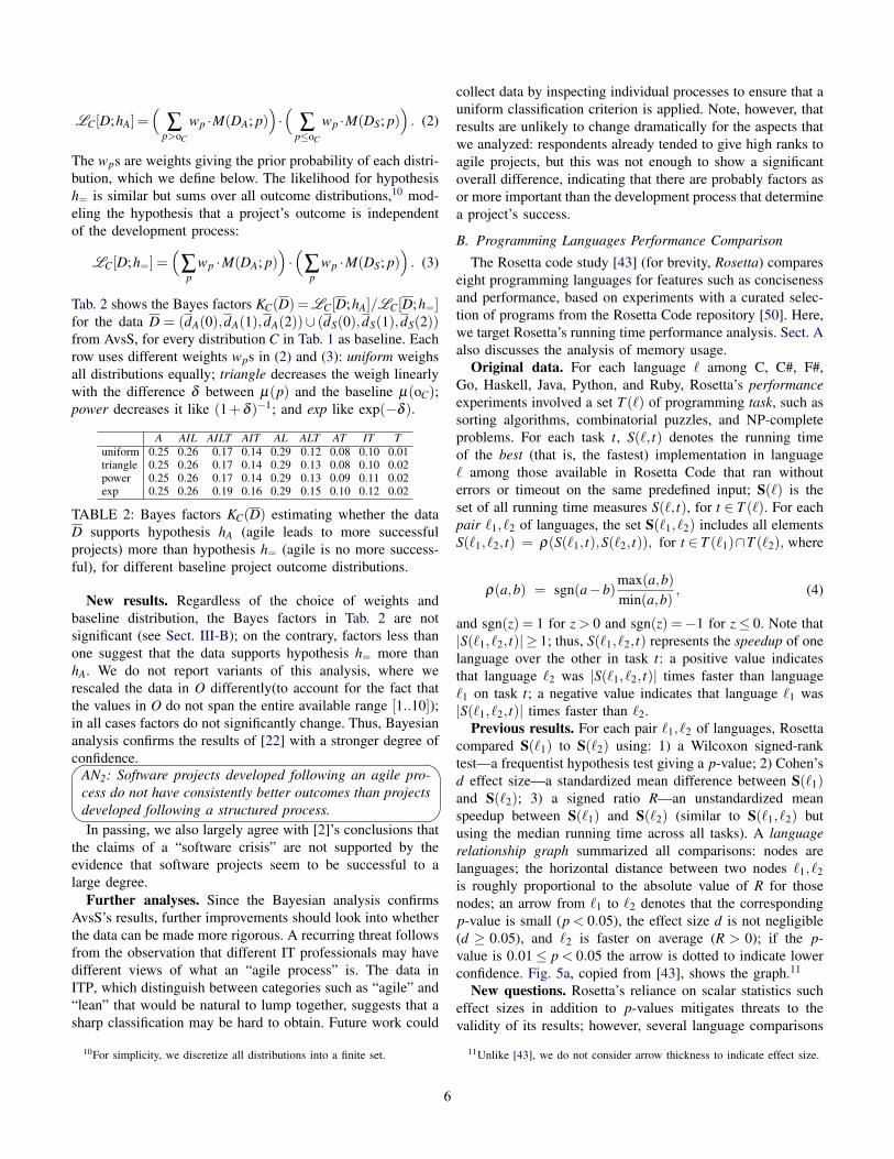
Tab. 2 shows the Bayes factors KC(D) =LC[D;hA]/LC[D;h=]for the data D = (dA(0),dA(1),dA(2))∪ (dS(0),dS(1),dS(2))from AvsS, for every distribution C in Tab. 1 as baseline. Eachrow uses different weights wps in (2) and (3): uniform weighsall distributions equally; triangle decreases the weigh linearlywith the difference δ between µ(p) and the baseline µ(oC);power decreases it like (1+δ )−1; and exp like exp(−δ ).

A AIL AILT AIT AL ALT AT IT Tuniform 0.25 0.26 0.17 0.14 0.29 0.12 0.08 0.10 0.01triangle 0.25 0.26 0.17 0.14 0.29 0.13 0.08 0.10 0.02power 0.25 0.26 0.17 0.14 0.29 0.13 0.09 0.11 0.02exp 0.25 0.26 0.19 0.16 0.29 0.15 0.10 0.12 0.02

TABLE 2: Bayes factors KC(D) estimating whether the dataD supports hypothesis hA (agile leads to more successfulprojects) more than hypothesis h= (agile is no more success-ful), for different baseline project outcome distributions.

New results. Regardless of the choice of weights andbaseline distribution, the Bayes factors in Tab. 2 are notsignificant (see Sect. III-B); on the contrary, factors less thanone suggest that the data supports hypothesis h= more thanhA. We do not report variants of this analysis, where werescaled the data in O differently(to account for the fact thatthe values in O do not span the entire available range [1..10]);in all cases factors do not significantly change. Thus, Bayesiananalysis confirms the results of [22] with a stronger degree ofconfidence.��

��

AN2: Software projects developed following an agile pro-cess do not have consistently better outcomes than projectsdeveloped following a structured process.In passing, we also largely agree with [2]’s conclusions that

the claims of a “software crisis” are not supported by theevidence that software projects seem to be successful to alarge degree.

Further analyses. Since the Bayesian analysis confirmsAvsS’s results, further improvements should look into whetherthe data can be made more rigorous. A recurring threat followsfrom the observation that different IT professionals may havedifferent views of what an “agile process” is. The data inITP, which distinguish between categories such as “agile” and“lean” that would be natural to lump together, suggests that asharp classification may be hard to obtain. Future work could

10For simplicity, we discretize all distributions into a finite set.

collect data by inspecting individual processes to ensure that auniform classification criterion is applied. Note, however, thatresults are unlikely to change dramatically for the aspects thatwe analyzed: respondents already tended to give high ranks toagile projects, but this was not enough to show a significantoverall difference, indicating that there are probably factors asor more important than the development process that determinea project’s success.

B. Programming Languages Performance Comparison

The Rosetta code study [43] (for brevity, Rosetta) compareseight programming languages for features such as concisenessand performance, based on experiments with a curated selec-tion of programs from the Rosetta Code repository [50]. Here,we target Rosetta’s running time performance analysis. Sect. Aalso discusses the analysis of memory usage.

Original data. For each language ` among C, C#, F#,Go, Haskell, Java, Python, and Ruby, Rosetta’s performanceexperiments involved a set T (`) of programming task, such assorting algorithms, combinatorial puzzles, and NP-completeproblems. For each task t, S(`, t) denotes the running timeof the best (that is, the fastest) implementation in language` among those available in Rosetta Code that ran withouterrors or timeout on the same predefined input; S(`) is theset of all running time measures S(`, t), for t ∈ T (`). For eachpair `1, `2 of languages, the set S(`1, `2) includes all elementsS(`1, `2, t) = ρ(S(`1, t),S(`2, t)), for t ∈ T (`1)∩T (`2), where

ρ(a,b) = sgn(a−b)max(a,b)min(a,b)

, (4)

and sgn(z) = 1 for z > 0 and sgn(z) =−1 for z≤ 0. Note that|S(`1, `2, t)| ≥ 1; thus, S(`1, `2, t) represents the speedup of onelanguage over the other in task t: a positive value indicatesthat language `2 was |S(`1, `2, t)| times faster than language`1 on task t; a negative value indicates that language `1 was|S(`1, `2, t)| times faster than `2.

Previous results. For each pair `1, `2 of languages, Rosettacompared S(`1) to S(`2) using: 1) a Wilcoxon signed-ranktest—a frequentist hypothesis test giving a p-value; 2) Cohen’sd effect size—a standardized mean difference between S(`1)and S(`2); 3) a signed ratio R—an unstandardized meanspeedup between S(`1) and S(`2) (similar to S(`1, `2) butusing the median running time across all tasks). A languagerelationship graph summarized all comparisons: nodes arelanguages; the horizontal distance between two nodes `1, `2is roughly proportional to the absolute value of R for thosenodes; an arrow from `1 to `2 denotes that the correspondingp-value is small (p < 0.05), the effect size d is not negligible(d ≥ 0.05), and `2 is faster on average (R > 0); if the p-value is 0.01≤ p < 0.05 the arrow is dotted to indicate lowerconfidence. Fig. 5a, copied from [43], shows the graph.11

New questions. Rosetta’s reliance on scalar statistics sucheffect sizes in addition to p-values mitigates threats to thevalidity of its results; however, several language comparisons

11Unlike [43], we do not consider arrow thickness to indicate effect size.

6

remain inconclusive. For example, it is somewhat surprisingthat Rosetta could not ascertain that a compiled highly-optimized language like Haskell is generally faster than thedynamic scripting languages Python and Ruby. We would alsolike to track down the impact of experimental choices thatdepended on factors Rosetta could not fully control for, suchas which implementations were available in Rosetta Code.

RQ1: Which programming languages have better runningtime performance, after taking into account the potentialsources of bias in Rosetta’s experimental data [43]?Additional data (benchmarks). As additional data on

performance and memory usage we consider the ComputerLanguage Benchmarks Game [56] (for brevity, Bench). Thedata from Bench are comparable to those from Rosetta asthey both consist of curated selections of collectively writtensolutions to well-defined programming tasks running on thesame input and refined over a significant stretch of time;12

on the other hand, Bench was developed independently ofRosetta, which makes it a complementary source of data.

For each language `, Bench’s performance experimentsdetermine a set S(`) with elements S(`, t,n,v), for t rangingover the set T (`) of Bench’s tasks, n ranging over the setN(`, t) of input sizes of task t in `, and v ranging over the setV (`, t) of different implementations of the same task t in `.Bench’s tasks include numerical algorithms, regular expressionmatching, and algorithms on trees. Bench’s performance datainclude experiments with different solutions for the same taskand inputs of different sizes; we avail this to model the possiblevariability in performance measurements. For each pair `1, `2of languages, the set S(`1, `2) includes all elements

S(`1, `2, t) = ρ

(min

v∈V (`1,t)S(`1, t,m,v), min

v∈V (`2,t)S(`2, t,m,v)

),

for t ∈ T (`1)∩ T (`2) and m = max(N(`1, t)∩N(`2, t)); thatis, S(`1, `2, t) is the speedup ratio (4) of the fastest solutionin `1 over the fastest solution in `2 for the same task t andrunning over the largest input that both languages can handle.Thus, S(`1, `2) is directly comparable to S(`1, `2) as the similarnotation suggests.

We also define the set S∆(`1, `2, t) of all valuesρ(S(`1, t,n,v1),S(`1, t,n,v2))−S(`1, `2, t), for n ranging overN(`1, t)∩N(`2, t), v1 ranging over V (`1, t), and v2 rangingover V (`2, t); intuitively, S∆(`1, `2, t) is the distribution ofall differences in speedup measurements for task t betweenany two programs (on input of any size) and the two fastestprograms (on the largest input). S∆(`1, `2, t) gives an idea ofthe variability in speedup ratios that may result from inputs orprograms other than those that turned out to be the fastest.

Bayesian analysis. For every pair `1, `2 of languages, theprior distribution πS(`1, `2) gives the probability πS(`1, `2)[r]of observing a program in `1 and a program in `2—solvingthe same problem and input—respectively running for t1 andt2 time units such that ρ(t1, t2) = r. Informally, the prior

12Some details of the performance measures are also similar, such as thechoice of including the Java VM startup time in the running time measures.

models the initial expectations on the performance differencebetween languages—which one will be faster and how much.We base our initial expectations on the results of Bench;hence, πS(`1, `2) follows the distribution of S(`1, `2). Precisely,S(`1, `2) is based on a finite number of discrete observations,and hence it excludes values that are perfectly acceptable butdid not happen to occur in the experiments. But if, say, `2 istwice as fast as `1 in an experiment and three times as fast inanother experiment, we expect speedup values between 2 and 3to be possible even if they were not observed in any performedexperiment. Thus, πS(`1, `2) is the kernel density estimation(KDE [58] using a normal kernel function13) of S(`1, `2);furthermore, we rework the smooth distribution obtained byKDE to exclude values in the interval (−1,1] since these areimpossible given the definition of ρ in (4).

The likelihood L S(`1, `2)[d;h] expresses how likely ob-serving a speedup d is, under the hypothesis that the actualspeedup is h. We base it on Bench’s extended experimentsfollowing this argumentation. The outcome of performanceexperiments also depends on some parameters, such as theinput size and specific implementation choices, that are some-what accidental; for example, Rosetta’s experiments usedinputs of significant size, manually selected; these choicesseem reasonable, but we cannot exclude that, if input sizeshad been chosen differently, the performance results wouldhave been quantitatively different. In order to assess thisexperimental uncertainty due to effects that cannot be entirelycontrolled, we base the likelihood on the values S∆(`1, `2, t),which span the differences between the reported data S(`1, `2)and the same metric for different choices of input size orprogram variant. Similarly to what we did for the prior, wesmooth the distribution of values

⋃t S∆(`1, `2, t) using KDE14,

which yields a probability density function ∆(`1, `2). Then,the likelihood L S(`1, `2)[d;h] ∝ ∆(`1, `2)[d − h] is a valueproportional to the probability of observing the difference d−hof speedups.

The posterior distribution PSS(`1, `2) is obtained by updat-

ing the prior (Sect. III-B) with Rosetta’s data S; PSS(`1, `2)[r]

is the probability that the speedup of `1 over `2 is r. Tab. 4summarizes the posteriors using two statistics: CI is the 95%credible interval15 (that is, there is a 95% chance that the realspeedup falls in the interval), and m is the median.16 Credibleintervals that include 0 may indicate an inconclusive compar-ison (one or the other language may be faster) One advantageof Bayesian analysis is that it provides distributions (ratherthan just scalar summaries), so that we can sort out borderlinecases by visually inspecting them. For example, Fig. 3 suggeststhat the Java vs. Python comparison is indeed inconclusive(there’s significant probability on both sides of the origin),whereas the F# vs. Ruby comparison has a very sharp peaknext to 1, which suggests that Ruby was consistently faster

13We used Python’s scipy.stats.gaussian_kde function.14We take the union over all tasks in Bench because they differ from

Rosetta’s.15Credible intervals are Bayesian analogues of confidence intervals.16The means are generally close to the medians.

7

−30 −25 −20 −15 −10 −5 0 5runtime ratio

0.0000

0.0005

0.0010

0.0015

0.0020

0.0025

prob

abili

ty

Java/PythonJava/Python (post)

−30 −25 −20 −15 −10 −5 0 5runtime ratio

0.000

0.005

0.010

0.015

0.020

0.025

prob

abili

ty

F#/RubyF#/Ruby (post)

Fig. 3: Posterior distributions PSS of running time ratios of Java vs. Python (left) and F# vs. Ruby (right).

than F#—albeit not much faster. We summarize the results ofthe posteriors’ analysis in the language relationship graph inFig. 5b. It conveys the same general information as the graphin Fig. 5a from [43], but it is based on Bayesian analysis; now,a dotted arrow indicates a speedup relationship that is weakor borderline but still likely to hold (such as F# vs. Ruby).

LANGUAGE C C# F# Go Haskell Java PythonC# CI (-10.1, -8.7)

m -9.22F# CI (-76.0, -64.5) (-8.9, -4.6)

m -72.61 -5.29Go CI (-2.3, -1.3) (1.0, 2.5) (16.9, 20.6)

m -1.67 1.15 18.21Haskell CI (-5.9, -5.7) (1.2, 1.7) (3.2, 15.5) (2.4, 2.5)

m -5.76 1.23 6.77 2.49Java CI (-3.2, -3.1) (-2.0, -1.3) (5.7, 7.5) (-8.5, -7.6) (-8.6, -8.3)

m -3.18 -1.77 6.94 -8.02 -8.63Python CI (-54.2, -32.3) (-1.4, 1.8) (2.1, 12.7) (-27.2, -17.7) (-5.0, -1.2) (-2.1, 2.2)

m -52.47 1.3 7.93 -23.01 -1.82 1.76Ruby CI (-124.0, -90.9) (-21.1, -11.6) (1.0, 1.1) (-142.2, -36.9) (-22.0, -19.9) (-17.0, -8.6) (-19.7, -14.0)

m -100.69 -16.96 1.05 -141.92 -21.85 -15.32 -15.03

TABLE 4: Comparison of running time: each cell in column`1 and row `2 reports the 95% credible interval CI and themedian m of the posterior distribution PS

S(`1, `2).

New results. Compared with Rosetta’s frequentist analy-sis [43], the overall picture emerging from Bayesian analysisis richer and somewhat more nuanced. C remains the king ofspeed, but Go cannot claim to stand out as lone runner up:Haskell is faster than Go on average (it was slower in theprevious analysis), even though the performance advantage ofC over Haskell is still greater than its advantage over Go.On the other hand, several comparisons that were surprisinglyinconclusive in Rosetta are now more clearly defined. Haskellemerges as faster than the scripting languages (Python andRuby) and than the bytecode object-oriented languages (C#and Java). In the opposite direction, F# has shown a generallypoor performance—in particular, quite slower than C# even ifthey both run on the same .NET platform. These differencesindicate that a few results of Rosetta hinged on contingentexperimental details; Bayesian analysis has lessened the biasby incorporating an independent data source.�

�

�

�

AN1: C is the king of performance. Go and Haskell (whichcompile to native) are the runner-ups. Object-orientedlanguages (C#, Java) retain a competitive performance onseveral tasks even if they compile to bytecode. Interpretedscripting languages (Python, Ruby) tend to be the slowest.Further analyses. Since Bayesian analysis relies on the data

from Bench, further analysis could try different sources for theprior and likelihood distributions, in order to understand thesensitivity of the analysis on the particular choice that wasdone. Bench, however, was chosen because it is the only datawe could find that is publicly available, described in detail,and sufficiently similar to Rosetta to be comparable to it; thusgetting more data may require to perform new experiments.

Another natural continuation of this work could collect ad-ditional data specifically for the comparisons where significantuncertainty remains. More data about C is probably redundantas its role as performance king is largely undisputed. Incontrast, F#’s data are unsatisfactory because they often showa large variability and disappointing results for a languagethat compiles to the same .NET platform as C#; more datawould help explain whether F#’s performance gap is intrinsic,or mainly due to a less mature language support.

C. Testing with Specifications

The Testing with Strong Specifications paper [49] (forbrevity, ST) assesses the effectiveness of random testing usingas oracles functional specifications in the form of assertionsembedded in the code (contracts).

Original data. ST’s experiments targeted the EiffelBaselibrary, comprising 21 classes implementing data structures—such as arrays, lists, hash tables, and trees—and iterators. STtested EiffelBase twice using the same random tester AutoTest:once using the simple specifications that come with Eiffel-Base’s code, and once using stronger specifications writtenas part of ST’s research. For each class Ck, k = 1, . . . ,21,testing using simple specifications detected tk bugs, whereastesting using strong specifications detected Tk bugs. These areactual specification violations that expose genuinely incorrectbehavior. t = t1, . . . , t21 and T = T1, . . . ,T21 are the sets of allbugs found using simple and using strong specifications.

Previous results. ST compared t to T using a Wilcoxonsigned-rank test—a frequentist hypothesis test giving a p-value0.006, which lead to rejecting the null hypothesis that usingsimple specifications and using strong specifications makesno difference in testing effectiveness. Also based on otherdata—such as the effort spent writing strong specifications—ST argued that strong specifications bring significant benefitsto random testing and achieve an interesting trade-off between

8

CC#

F#

Go

Haskell

Java

Python

Ruby

(a) Previous analysis [43].

C

C#F#

Go

Haskell

Java

Python

Ruby

(b) Bayesian analysis.

Fig. 5: Comparison of running time: qualitative summaries.

effort and bug-detection effectiveness.New questions. ST’s analysis is quite convincing as it

stands, because it is based on analyses other than hypothesistesting; rather than confirming its results using Bayesianstatistics, we extend its analysis into a different direction:studying the distribution of bugs in classes.

RQ3: What is the distribution of bugs in classes? Does itsatisfy the Pareto principle: “80% of the bugs are locatedin only 20% of the classes”, or, conversely, “80% of theclasses are affected by only 20% of the bugs”?Additional data. Zhang suggested [62] that bug distribu-

tions in modules follow a Weibull—a continuous distribu-tions with positive parameters α and β , p.d.f. wα,β [x] =

(β/α)(x/α)β−1 exp(−(x/α)β ) and c.d.f.17

Wα,β [x] = 1− exp(−( x

α

)β). (5)

Saying that the bug distribution in modules follows a Weibullwith c.d.f. (5) means that a fraction Wα,β [x] of the moduleshas x or fewer bugs; or, equivalently, that a random modulehas x or fewer bugs with probability Wα,β [x]. Under theseconditions, the Pareto principle would hold only for certainvalues of α and β : while β determines the distribution’s shape,and hence qualitative properties such as the Pareto principle,α determines the distribution’s scale, and hence only specificquantitative properties.

Bayesian analysis: Pareto principle. Classes are modulesin object-oriented programs; thus, we can use Bayes theoremto estimate α and β such that a Weibull with c.d.f. Wα,β

fits the distribution of bugs T detected using strong spec-ifications. Using Bayesian analysis, we infer a multivariatedistribution m of values for parameters α and β . Since wehave no inkling of plausible values for α and β , we use anuninformative uniform prior π[α,β ] ∝ 1 for all α,β within abroad range. The likelihood L [d;α,β ] reflects the probabilitythat d is drawn from a Weibull with parameters α and β ; thusL [d;α,β ] ∝ wα,β [d + 1], where we shift the p.d.f. by oneunit to account for classes with no bugs. By applying Bayestheorem, the joint posterior distribution is:

m[α,β ] = PT[α,β ] = ν ∏d∈T

wα,β [d +1] ,

where ν is a normalization factor obtained by the, by nowfamiliar, update rule (Sect. III-B), using data T from testingwith strong specifications. Fig. 6 shows m’s marginals m[α]

17A cumulative distribution function (c.d.f.) X [x] gives P[X ≤ x].

0 5 10 15 20values of parameters α,β

0.000

0.002

0.004

0.006

0.008

0.010

0.012

0.014

0.016

prob

abili

ty

α̂ = 7.64

αh90 = 12.83

α l90 = 5.31

β̂ = 0.82

β h90 = 1.08

β l90 = 0.74

α

β

Fig. 6: Marginals m[α] and m[β ] of the posterior distributionm[α,β ] of parameters α and β . The graph indicates maximaα̂ and β̂ and 90% credible intervals (α l

90,αh90) and (β l

90,βh90).

and m[β ].18 The plot indicates that there is limited uncertaintyabout the value of β , whereas the uncertainty about α issignificant. In terms of the resulting Weibull distributions, theuncertainty is mainly on the scale of the distribution (param-eter α) but not so much on its shape (parameter β ). Fig. 7shows this by plotting the Weibull’s c.d.f. Wα,β for parametersin the 90% credible intervals highlighted in Fig. 6. The picturesuggests that the Pareto principle holds: the number b of bugssuch that Wα,β [b] = 0.8 is 8%, 10%, and 13% of the totalnumber of possible bugs—one percentage for each choice ofα,β in Fig. 7—which is in the ballpark of Pareto’s 80–20proportion. The qualitative conclusions wouldn’t change if weused data t from testing with simple specifications.��

��

AN3-A: The distribution across classes of bugs found byrandom testing with specifications is modeled accuratelyby a Weibull distribution that satisfies the Pareto principle.A significant advantage of Bayesian analysis over using

frequentist statistics is that we have distributions of likelyparameter values, not just pointwise estimates. This entails thatwe can derive distributions of related variables. For example,we could plot how the probability of finding a class with atmost N bugs–for any given N—varies with α and β . SeeSect. C for an example of this.

Bayesian analysis: total bugs. This analysis modeled thenumber of bugs found by random testing; what about the totalnumber of bugs present in a class? Can we use Bayesiananalysis to estimate it as well?

As a first step, suppose that the effectiveness of random

18The maxima are close to means (µ(m[α]) = 8.53, µ(m[β ]) = 0.88) andmedians (m(m[α]) = 6.86 and m(m[β ]) = 0.81).

9

0 20 40 60 80 100 120 140 160# bugs

0.0

0.2

0.4

0.6

0.8

1.0

prob

abili

ty/f

ract

ion

α l90,β

l90

α̂, β̂

αh90,β

h90

Fig. 7: Cumulative distribution function Wα,β (5) for thedifferent values of α and β highlighted in Fig. 6.

testing with strong specifications is E: if testing finds Nbugs—a fraction E of the total—there are actually N/Ebugs in the class. Similarly, let e be the effectiveness ofrandom testing with simple specifications. Given E and e, wecan estimate the distribution B of real bugs using Bayesiananalysis. The prior distribution has p.d.f. πb(α,β ,E) suchthat πb(α,β ,E)[x] = wα,β [x ·E], corresponding to a Weibullscaled so as to follow the expected actual bugs. The likelihoodL b(e)[d;h] is proportional to the probability that testing witheffectiveness e finds d bugs in a class with h total bugs;thus, L b(e)[d;h] ∝ B(h,e)[d], where B(h,e) is the binomialdistribution’s p.m.f. giving the probability of d successes(d bugs found) out of h attempts when each attempt hasprobability e of success. With these prior and likelihood, theposterior distribution Pb

d (α,β ,e,E)[x] =Bα,β (d,e,E)[x] givesthe probability that a class has a total of x bugs given thattesting with effectiveness e found d bugs (and testing witheffectiveness E determined a Weibull with parameters α,β ).

This analysis requires knowing plausible values for α

and β—which we can obtain from the previous analysissummarized in Fig. 6—as well as for e and E—which isinstead the rub of the analysis. Fortunately, we can addone layer of Bayesian inference to abstract over the un-known effectiveness values. The uninformative prior πn

α,β (d)is now a uniform distribution over distributions such thatπn

α,β (d)[e,E] is the probability associated with Bα,β (d,e,E)defined in the previous analysis. The likelihood L n[d;e,E]measures the probability that testing modeled by a distributionwith parameters e,E finds d bugs in a class: L n[d;e,E] ∝

∑h L b(e)[d;h] · Bα,β (d,e,E)[h]. With the usual update rule,compute the posterior Pα,β

d [e,E] given values for α , β , anda number of bugs d detected in some class. Finally, Nα,β

m [n],which gives the probability that class m has n bugs, is amixture that interpolates posteriors:

Nα,βd [n] = ∑

e,EBα,β (d,e,E)[n] ·Pα,β

d [e,E] ,

where d is the number of bugs found in a class by testing witheffectiveness e.

C1 C2 C3 C4 C5 C6 C7 C8 C9 C10 C11 C12 C13 C14 C15 C16 C17 C18 C19 C20 C21m/|M| 0.27 0.03 0.20 0.38 0.52 0.17 0.15 0.15 0.39 0.23 0.11 0.15 0.43 0.15 1.04 0.08 0.15 0.51 0.15 1.21 0.67m(N) 14 3 5 19 38 5 10 2 31 20 5 3 22 13 22 8 1 71 3 67 2Nl

90 5 0 2 18 20 2 2 0 2 2 2 0 22 0 4 4 0 25 0 49 0

Nh90 26 7 17 54 57 17 17 7 17 17 17 7 60 7 22 22 7 66 7 100 7

TABLE 8: Median per public method m/|M|, median m(N),

and 90% credible interval (Nl90,N

h90) of Nα̂,β̂

dm—estimating the

total number of bugs in class Cm.

Tab. 8 shows statistics about Nα̂,β̂dm

for all 21 classes analyzedin ST. The parameters α = α̂ and β = β̂ are the maximumlikelihood values in Fig. 6; prior effectiveness ranges over0.15≤ e≤ 0.5 for testing with simple specifications and over0.7 ≤ E ≤ 0.95 for testing with strong specifications; anddm = tm, for m = 1, . . . ,21, is the number of bugs foundin class Cm by testing with simple specifications in ST’sexperiments. The median bugs per public method—similar tobugs per function point [35]—is an indicator of bug pronenessconsidered more robust than bugs per line of code. Accordingto this metric, trees (class C20) and linked stacks (class C15)data structures are the faultiest, while arrayed lists (class C2)and linked lists (class C11) are the least faulty. The differencecan be explained in terms of which structures are the mostused in Eiffel programs: lists are widely used, and hence theirimplementations have been heavily tested and fixed.��

��

AN3-B: The number of total bugs in a class can be estimatedby Bayesian analysis from the bugs found by randomtesting. Classes that are less used are more error prone.Further analyses. Using Bayesian analysis we obtained a

reliable estimate of the real bugs present in a data structurelibrary; there remains a significant margin of uncertainty,given that we abstracted over several unknown details, butthe uncertainty is quantified and upheld by precise modelingchoices. Generalizing the analysis to include other testingtechniques (e.g., manual testing) or, conversely, specialize itto other domains and conditions to make it more preciseare natural extensions of this work. We used a very simplemodel of testing effectiveness based on detection effectiveness;using more detailed models of random testing [5] may provideadditional insights and more accurate estimates.

V. THREATS TO VALIDITY

Do Bayesian techniques help with mitigating threats tovalidity? To answer this question, we consider each of theusual kinds of threats (construct, conclusion, internal, andexternal), and assess them for the case studies in Sect. IV.

Bayesian analysis is unlikely to affect construct validity,which has to do with whether we measured what the studywas supposed to measure. This threat is very limited forthe programming language and testing studies (Sect. IV-Band Sect. IV-C), which target well-defined and understoodmeasures (running time, number of bugs). It is potentiallymore significant for the agile vs. structured study, becauseclassifying processes in only two categories (agile and struc-tured) may be partly fuzzy and subjective; however, Sect. IV-Adiscusses how the analysis is quite robust w.r.t. how thisclassification is done, which gives us confidence in its results.

10

Conclusion validity depends on the application of appropri-ate statistical tests. As we discuss in Sect. III-B, frequentisthypothesis testing techniques are questionable because theydo not properly assess significance; switching to Bayesiananalysis can certainly help in this respect. Thus, conclusionvalidity threats are lower in our three case studies than in theoriginal studies that provided the data.

Internal validity is mainly concerned with whether causalityis correctly evaluated. This depends on several details ofexperimental design that are generally independent of whetherfrequentist or Bayesian statistics are used. One importantaspect of internal validity pertains to the avoidance of bias;this is where Bayesian statistics can help, thanks to its abilityof weighting out many different competing models rather thanrestricting the analysis to two predefined hypotheses (null vs.alternative hypothesis). This aspect is particularly relevant forthe agile vs. structured study in the way it uses Bayes factors.

Since it integrates previous, or otherwise independentlyobtained, information in the form or priors, Bayesian analysiscan help mitigate threats to external validity, which concernthe generalizability of findings. Using an informative priormakes the statistics reflect not just the current experimentaldata but also prior knowledge and assumptions on the subject;conversely, being able to get to the same conclusions usingdifferent, uninformative priors indicates that the experimentalevidence is strong over initial assumptions. In both cases,Bayesian statistics support analyses where generalizability ismore explicitly taken into account instead of being just anafterthought. This applies to all three case studies, and inparticular to the programming language performance analysis(Sect. IV-B) which integrated independent information to boostthe confidence in the results.

VI. PRACTICAL GUIDELINES

We conclude by summarizing practical guidelines to per-form Bayesian analysis on empirical data from diversesoftware-engineering research.• If previous studies on the same subject are available,

consider incorporating their data into the analysis in theform of prior—if only to estimate to what extent theinterpretation of the new results changes according towhat prior is used.

• To allow other researchers to do the same with your data,make it available in machine-readable form in addition tostatistics and visualizations.

• Try to compute distributions of estimates rather thanonly single-point estimates. Visualize data as well as thecomputed distributions, and use the visual information todirect and refine your analysis.

• Consider alternatives to statistical hypothesis testing, forexample the computation of Bayes factors; in any case,do not rely solely on the p-value to draw conclusions.

• More generally, avoid phrasing your analysis in termsof binary antithetical choices. No statistical tests cansubstitute careful, informed modeling of assumptions.

11

REFERENCES

[1] Scott W. Ambler. Ambysoft’s IT project success rates survey results.http://www.ambysoft.com/surveys/success2013.html, December 2013.

[2] Scott W. Ambler. The non-existent software crisis: Debunking thechaos report. Dr. Dobb’s, February 2014. http://www.drdobbs.com/architecture-and-design/the-non-existent-software-crisis-debunki/240165910.

[3] Andrea Arcuri and Lionel C. Briand. A practical guide for usingstatistical tests to assess randomized algorithms in software engineer-ing. In Proceedings of the 33rd International Conference on SoftwareEngineering (ICSE 2011), pages 1–10. ACM, 2011.

[4] Andrea Arcuri and Lionel C. Briand. A hitchhiker’s guide to statisticaltests for assessing randomized algorithms in software engineering. Softw.Test., Verif. Reliab., 24(3):219–250, 2014.

[5] Andrea Arcuri, Muhammad Zohaib Z. Iqbal, and Lionel C. Briand.Random testing: Theoretical results and practical implications. IEEETrans. Software Eng., 38(2):258–277, 2012.

[6] Alberto Bacchelli and Christian Bird. Expectations, outcomes, andchallenges of modern code review. In Notkin et al. [45], pages 712–721.

[7] David Barber. Bayesian Reasoning and Machine Learning. CambridgeUniversity Press, 2012.

[8] Gabriele Bavota, Bogdan Dit, Rocco Oliveto, Massimiliano Di Penta,Denys Poshyvanyk, and Andrea De Lucia. An empirical study on thedevelopers’ perception of software coupling. In Notkin et al. [45], pages692–701.

[9] Andrew Begel and Nachiappan Nagappan. Pair programming: what’sin it for me? In Proceedings of the Second International Symposiumon Empirical Software Engineering and Measurement (ESEM), pages120–128. ACM, 2008.

[10] A. Bener and A. Tosun. If it is softare engineering, it is (probably) aBayesian factor. In Menzies et al. [40].

[11] Antonia Bertolino, Gerardo Canfora, and Sebastian G. Elbaum, editors.37th IEEE/ACM International Conference on Software Engineering,ICSE 2015, Volume 1. IEEE Computer Society, 2015.

[12] Thirumalesh Bhat and Nachiappan Nagappan. Evaluating the efficacy oftest-driven development: industrial case studies. In 2006 InternationalSymposium on Empirical Software Engineering (ISESE), pages 356–363.ACM, 2006.

[13] Nélio Cacho, Thiago César, Thomas Filipe, Eliezio Soares, Arthur Cas-sio, Rafael Souza, Israel García, Eiji Adachi Barbosa, and AlessandroGarcia. Trading robustness for maintainability: an empirical study ofevolving C# programs. In Jalote et al. [32], pages 584–595.

[14] Junjie Chen, Wenxiang Hu, Dan Hao, Yingfei Xiong, Hongyu Zhang,Lu Zhang, and Bing Xie. An empirical comparison of compiler testingtechniques. In Dillon et al. [20], pages 180–190.

[15] Shauvik Roy Choudhary, Mukul R. Prasad, and Alessandro Orso. X-PERT: accurate identification of cross-browser issues in web applica-tions. In Notkin et al. [45], pages 702–711.

[16] Jacob Cohen. Statistical power analysis for the behavioral sciences.Academic Press, 1969.

[17] Jacob Cohen. The earth is round (p < .05). American Psychologist,49(12):997–1003, 1994.

[18] Confusion of the inverse. http://rationalwiki.org/wiki/Confusion_of_the_inverse, February 2016.

[19] Premkumar T. Devanbu, Thomas Zimmermann, and Christian Bird.Belief & evidence in empirical software engineering. In Dillon et al.[20], pages 108–119.

[20] Laura K. Dillon, Willem Visser, and Laurie Williams, editors. Pro-ceedings of the 38th International Conference on Software Engineering,ICSE 2016. ACM, 2016.

[21] Allen B. Downey. Think Bayes. O’Reilly Media, 2013.[22] H.-Christian Estler, Martin Nordio, Carlo A. Furia, Bertrand Meyer,

and Johannes Schneider. Agile vs. structured distributed softwaredevelopment: A case study. In Proceedings of the 7th InternationalConference on Global Software Engineering (ICGSE’12), pages 11–20.IEEE, 2012.

[23] Hans-Christian Estler, Martin Nordio, Carlo A. Furia, Bertrand Meyer,and Johannes Schneider. Agile vs. structured distributed software de-velopment: A case study. Empirical Software Engineering, 19(5):1197–1224, 2014.

[24] David Silver et al. Mastering the game of Go with deep neural networksand tree search. Nature, 429:484–489, 2016.

[25] Andrew Gelman. The problems with p-values are not just with p-values.The American Statistician, 2016. Online discussion: http://www.stat.columbia.edu/~gelman/research/published/asa_pvalues.pdf.

[26] Irving John Good. Explicativity, corroboration, and the relative odds ofhypotheses. Synthese, 30(1/2):39–73, 1975.

[27] Steven N. Goodman. Toward evidence-based medical statistics. 1: Thep value fallacy. Annals of Internal Medicine, 130(12):995–1004, 1999.

[28] Chris Bambey Guure, Noor Akma Ibrahim, and Al Omari MohammedAhmed. Bayesian estimation of two-parameter Weibull distributionusing extension of Jeffreys’ prior information with three loss functions.Mathematical Problems in Engineering, 2012. http://dx.doi.org/10.1155/2012/589640.

[29] Trevor Hastie, Robert Tibshirani, and Jerome Friedman. The Elements ofStatistical Learning: Data Mining, Inference, and Prediction. Springer,2nd edition, 2009.

[30] Hanna Hulkko and Pekka Abrahamsson. A multiple case study on theimpact of pair programming on Product Quality. In 27th InternationalConference on Software Engineering (ICSE), pages 495–504. ACM,2005.

[31] John P. A. Ioannidis. Why most published research findings are false.PLoS Med, 2(8), 2005.

[32] Pankaj Jalote, Lionel C. Briand, and André van der Hoek, editors. 36thInternational Conference on Software Engineering, ICSE ’14. ACM,2014.

[33] Andreas Jedlitschka, Natalia Juristo Juzgado, and H. Dieter Rombach.Reporting experiments to satisfy professionals’ information needs. Em-pirical Software Engineering, 19(6):1921–1955, 2014.

[34] Harold Jeffreys. Theory of Probability. Oxford Classic Texts in thePhysical Sciences. Oxford University Press, 3rd edition, 1998.

[35] Capers Jones. Function points as a universal software metric. ACMSIGSOFT Software Engineering Notes, 38(4):1–27, 2013.

[36] Miryung Kim, Thomas Zimmermann, Robert DeLine, and AndrewBegel. The emerging role of data scientists on software developmentteams. In Dillon et al. [20], pages 96–107.

[37] Miryung Kim, Thomas Zimmermann, Robert DeLine, and AndrewBegel. The emerging role of data scientists on software developmentteams. In Dillon et al. [20], pages 96–107.

[38] Irene Manotas, Christian Bird, Rui Zhang, David C. Shepherd, Ciera Jas-pan, Caitlin Sadowski, Lori L. Pollock, and James Clause. An empiricalstudy of practitioners’ perspectives on green software engineering. InDillon et al. [20], pages 237–248.

[39] Daniel Matichuk, Toby C. Murray, June Andronick, D. Ross Jeffery,Gerwin Klein, and Mark Staples. Empirical study towards a leadingindicator for cost of formal software verification. In Bertolino et al.[11], pages 722–732.

[40] Tim Menzies, Laurie Williams, and Thomas Zimmermann, editors. Per-spectives on Data Science for Software Engineering. Morgan Kaufmann,2016.

[41] Matthias M. Müller and Walter F. Tichy. Case study: Extreme pro-gramming in a university environment. In Proceedings of the 23rdInternational Conference on Software Engineering, ICSE, pages 537–544. IEEE, 2001.

[42] Sarah Nadi, Thorsten Berger, Christian Kästner, and Krzysztof Czar-necki. Mining configuration constraints: static analyses and empiricalresults. In Jalote et al. [32], pages 140–151.

[43] Sebastian Nanz and Carlo A. Furia. A comparative study of pro-gramming languages in Rosetta Code. In Proceedings of the 37thInternational Conference on Software Engineering (ICSE), pages 778–788. ACM, 2015.

[44] Jerzy R. Nawrocki, Bartosz Walter, and Adam Wojciechowski. Com-parison of CMM Level 2 and eXtreme Programming. In Proceedingsof the 7th Internation Conference on Software Quality (ECSQ), volume2349 of Lecture Notes in Computer Science, pages 288–297. Springer,2002.

[45] David Notkin, Betty H. C. Cheng, and Klaus Pohl, editors. 35thInternational Conference on Software Engineering, ICSE ’13. IEEEComputer Society, 2013.

[46] Sebastiano Panichella, Annibale Panichella, Moritz Beller, Andy Zaid-man, and Harald C. Gall. The impact of test case summaries on bugfixing performance: an empirical investigation. In Dillon et al. [20],pages 547–558.

[47] Mike Papadakis, Yue Jia, Mark Harman, and Yves Le Traon. Trivialcompiler equivalence: A large scale empirical study of a simple, fast

12

and effective equivalent mutant detection technique. In Bertolino et al.[11], pages 936–946.

[48] Marian Petre. UML in practice. In Notkin et al. [45], pages 722–731.[49] Nadia Polikarpova, Carlo A. Furia, Yu Pei, Yi Wei, and Bertrand

Meyer. What good are strong specifications? In Proceedings of the35th International Conference on Software Engineering (ICSE), pages257–266. ACM, May 2013.

[50] Rosetta code. http://rosettacode.org/, Aug 2016.[51] Marija Selakovic and Michael Pradel. Performance issues and opti-

mizations in JavaScript: an empirical study. In Dillon et al. [20], pages61–72.

[52] Janet Siegmund, Norbert Siegmund, and Sven Apel. Views on internaland external validity in empirical software engineering. In Bertolinoet al. [11], pages 9–19.

[53] Joseph P. Simmons, Leif D. Nelson, and Uri Simonsohn. False-positivepsychology. Psychological Science, 22(11):1359–1366, 2011.

[54] Klaas-Jan Stol, Paul Ralph, and Brian Fitzgerald. Grounded theory insoftware engineering research: a critical review and guidelines. In Dillonet al. [20], pages 120–131.

[55] Guoxin Su and David S. Rosenblum. Perturbation analysis of stochasticsystems with empirical distribution parameters. In Jalote et al. [32],pages 311–321.

[56] The computer language benchmarks game. http://benchmarksgame.alioth.debian.org/, Aug 2016.

[57] Phillip Merlin Uesbeck, Andreas Stefik, Stefan Hanenberg, Jan Pedersen,and Patrick Daleiden. An empirical study on the impact of C++ lambdasand programmer experience. In Dillon et al. [20], pages 760–771.

[58] M. P. Wand and M. C. Jones. Kernel Smoothing, volume 60 of Mono-graphs on Statistics and Applied Probability. Chapman & Hall/CRC,1994.

[59] Ronald L. Wasserstein and Nicole A. Lazar. The ASA’s statement onp-values: Context, process, and purpose. The American Statistician,70(2):129–133, 2016.

[60] Claes Wohlin, Per Runeson, Martin Höst, Magnus C. Ohlsson, and BjörnRegnell. Experimentation in Software Engineering. Springer, 2012.

[61] Aiko Fallas Yamashita and Leon Moonen. Exploring the impact ofinter-smell relations on software maintainability: an empirical study. InNotkin et al. [45], pages 682–691.

[62] Hongyu Zhang. On the distibution of software faults. IEEE Transactionson Software Engineering, 34(2):301–302, 2008.

[63] Hongyu Zhang, Liang Gong, and Steven Versteeg. Predicting bug-fixingtime: an empirical study of commercial software projects. In Notkinet al. [45], pages 1042–1051.

[64] Hao Zhong and Zhendong Su. An empirical study on real bug fixes. InBertolino et al. [11], pages 913–923.

13

APPENDIX

CONTENTS

I Introduction 1

II Related Work 2

III A Practical Overview of Bayesian Statistics 2III-A Bayes Theorem . . . . . . . . . . . . . . . . . . . . . . . . . . . . . . . . . . . . . . . . . . . . . . . . 3III-B Frequentist vs. Bayesian Statistics . . . . . . . . . . . . . . . . . . . . . . . . . . . . . . . . . . . . . . 3

IV Case Studies 4IV-A Agile vs. Structured Development . . . . . . . . . . . . . . . . . . . . . . . . . . . . . . . . . . . . . . 4IV-B Programming Languages Performance Comparison . . . . . . . . . . . . . . . . . . . . . . . . . . . . . 6IV-C Testing with Specifications . . . . . . . . . . . . . . . . . . . . . . . . . . . . . . . . . . . . . . . . . . 8

V Threats to Validity 10

VI Practical Guidelines 11

References 12

Appendix 14A Rosetta Code Study . . . . . . . . . . . . . . . . . . . . . . . . . . . . . . . . . . . . . . . . . . . . . . 16

A1 Running time . . . . . . . . . . . . . . . . . . . . . . . . . . . . . . . . . . . . . . . . . . . 16A2 Memory usage . . . . . . . . . . . . . . . . . . . . . . . . . . . . . . . . . . . . . . . . . . . 23

B Agile vs. Structured Study . . . . . . . . . . . . . . . . . . . . . . . . . . . . . . . . . . . . . . . . . . 30B1 Success . . . . . . . . . . . . . . . . . . . . . . . . . . . . . . . . . . . . . . . . . . . . . . . 30B2 Importance for customers . . . . . . . . . . . . . . . . . . . . . . . . . . . . . . . . . . . . . 30

C Testing Study . . . . . . . . . . . . . . . . . . . . . . . . . . . . . . . . . . . . . . . . . . . . . . . . . 32

LIST OF FIGURES

3 Posterior distributions PSS of running time ratios of Java vs. Python (left) and F# vs. Ruby (right). . . . . . . . 8

5 Comparison of running time: qualitative summaries. . . . . . . . . . . . . . . . . . . . . . . . . . . . . . . . . . 96 Marginals m[α] and m[β ] of the posterior distribution m[α,β ] of parameters α and β . The graph indicates maxima

α̂ and β̂ and 90% credible intervals (α l90,α

h90) and (β l

90,βh90). . . . . . . . . . . . . . . . . . . . . . . . . . . . . 9

7 Cumulative distribution function Wα,β (5) for the different values of α and β highlighted in Fig. 6. . . . . . . . 1010 Running time . . . . . . . . . . . . . . . . . . . . . . . . . . . . . . . . . . . . . . . . . . . . . . . . . . . . . . 1611 Running time (C vs. other languages) . . . . . . . . . . . . . . . . . . . . . . . . . . . . . . . . . . . . . . . . . 1712 Running time (C# vs. other languages) . . . . . . . . . . . . . . . . . . . . . . . . . . . . . . . . . . . . . . . . . 1813 Running time (F# vs. other languages) . . . . . . . . . . . . . . . . . . . . . . . . . . . . . . . . . . . . . . . . . 1914 Running time (Go vs. other languages) . . . . . . . . . . . . . . . . . . . . . . . . . . . . . . . . . . . . . . . . 2015 Running time (Haskell vs. other languages) . . . . . . . . . . . . . . . . . . . . . . . . . . . . . . . . . . . . . . 2116 Running time (Java vs. other languages) . . . . . . . . . . . . . . . . . . . . . . . . . . . . . . . . . . . . . . . . 2117 Running time (Python vs. other languages) . . . . . . . . . . . . . . . . . . . . . . . . . . . . . . . . . . . . . . 2218 Comparison of used memory: qualitative summaries. . . . . . . . . . . . . . . . . . . . . . . . . . . . . . . . . . 2320 Maximum RAM usage . . . . . . . . . . . . . . . . . . . . . . . . . . . . . . . . . . . . . . . . . . . . . . . . . 2321 Maximum RAM usage (C vs. other languages) . . . . . . . . . . . . . . . . . . . . . . . . . . . . . . . . . . . . 2422 Maximum RAM usage (C# vs. other languages) . . . . . . . . . . . . . . . . . . . . . . . . . . . . . . . . . . . 2523 Maximum RAM usage (F# vs. other languages) . . . . . . . . . . . . . . . . . . . . . . . . . . . . . . . . . . . . 2624 Maximum RAM usage (Go vs. other languages) . . . . . . . . . . . . . . . . . . . . . . . . . . . . . . . . . . . 2725 Maximum RAM usage (Haskell vs. other languages) . . . . . . . . . . . . . . . . . . . . . . . . . . . . . . . . . 2826 Maximum RAM usage (Java vs. other languages) . . . . . . . . . . . . . . . . . . . . . . . . . . . . . . . . . . . 2827 Maximum RAM usage (Python vs. other languages) . . . . . . . . . . . . . . . . . . . . . . . . . . . . . . . . . 2934 Marginals m[α] and m[β ] of the posterior distribution m[α,β ] of parameters α and β for uniform priors (left)

and for Jeffreys prior (right). . . . . . . . . . . . . . . . . . . . . . . . . . . . . . . . . . . . . . . . . . . . . . . 32

14

35 Cumulative distribution function Wα,β for the values of α and β in Fig. 34 for uniform priors (left) and forJeffreys prior (right). . . . . . . . . . . . . . . . . . . . . . . . . . . . . . . . . . . . . . . . . . . . . . . . . . . 33

36 Marginals of the probability distribution for a module having zero bugs detected by random testing with strongspecifications for the values of α and β in a 90% credible interval for uniform priors (left) and for Jeffreys prior(right). . . . . . . . . . . . . . . . . . . . . . . . . . . . . . . . . . . . . . . . . . . . . . . . . . . . . . . . . . . 33

37 Marginals of the probability distribution for a module having at most five bugs detected by random testing withstrong specifications for the values of α and β in a 90% credible interval for uniform priors (left) and for Jeffreysprior (right). . . . . . . . . . . . . . . . . . . . . . . . . . . . . . . . . . . . . . . . . . . . . . . . . . . . . . . . 34

38 Distributions Nm of total bugs in module Cm (starting with uniform priors to get values of α̂, β̂ for prior Weibull). 35

39 Distributions Nm of total bugs in module Cm (starting with uniform priors to get values of α̂, β̂ for prior Weibull). 36

40 Distributions Nm of total bugs in module Cm (starting with uniform priors to get values of α̂, β̂ for prior Weibull). 37

LIST OF TABLES

1 Data from ITP: for each column header C ⊆ {A, I,L,T}, oC[k] is the probability that the outcome of projectsfollowing processes in categories C is k ∈ [0..2]. . . . . . . . . . . . . . . . . . . . . . . . . . . . . . . . . . . . 5

2 Bayes factors KC(D) estimating whether the data D supports hypothesis hA (agile leads to more successful projects)more than hypothesis h= (agile is no more successful), for different baseline project outcome distributions. . . . 6

4 Comparison of running time: each cell in column `1 and row `2 reports the 95% credible interval CI and themedian m of the posterior distribution PS

S(`1, `2). . . . . . . . . . . . . . . . . . . . . . . . . . . . . . . . . . . 8

8 Median per public method m/|M|, median m(N), and 90% credible interval (Nl90,N

h90) of Nα̂,β̂

dm—estimating the

total number of bugs in class Cm. . . . . . . . . . . . . . . . . . . . . . . . . . . . . . . . . . . . . . . . . . . . 10

9 Comparison of running times . . . . . . . . . . . . . . . . . . . . . . . . . . . . . . . . . . . . . . . . . . . . . . 16

19 Comparison of maximum RAM usage . . . . . . . . . . . . . . . . . . . . . . . . . . . . . . . . . . . . . . . . . 23

28 Different distributions for the baseline probability of outcome for software projects: for C one of the subsets of{A, I,L,T} in the column headers, oC[k] is the probability that outcome is k ∈ {0,1,2} in processes of category C. 30

29 Bayes factors K estimating to what extent the hypothesis “agile leads to more successful projects” is supportedover the other hypothesis “agile is no better than structured”. . . . . . . . . . . . . . . . . . . . . . . . . . . . . 30

30 Different distributions for the baseline probability of customer importance for software projects: for C one of thesubsets of {A, I,L,T} in the column headers, ιC[k] is the probability that customer importance is k ∈ {0,1,2} inprocesses of category C. . . . . . . . . . . . . . . . . . . . . . . . . . . . . . . . . . . . . . . . . . . . . . . . . 30

31 Bayes factors K estimating to what extent the hypothesis “agile is used for projects that are more important forcustomers” is supported over the other hypothesis “agile is no better than structured”. . . . . . . . . . . . . . . . 31

32 For every class Cm, m = 1, . . . ,21, the mean µ(N), median m(N), maximum likelihood N̂, 90% credible interval(Nl

90,Nl90), ratio m(N)/LOC median to lines of code, and ratio m(N)/#R median to number of methods of the

distribution of total bugs in the class. The analysis started with α̂, β̂ given by the maximum likelihood for α,βin m[α,β ] computed from a uniform prior. . . . . . . . . . . . . . . . . . . . . . . . . . . . . . . . . . . . . . . 32

33 For every class Cm, m = 1, . . . ,21, the mean µ(N), median m(N), maximum likelihood N̂, 90% credible interval(Nl

90,Nl90), ratio m(N)/LOC median to lines of code, and ratio m(N)/#R median to number of methods of the

distribution of total bugs in the class. The analysis started with α̂, β̂ given by the maximum likelihood for α,βin m[α,β ] computed from Jeffreys prior. . . . . . . . . . . . . . . . . . . . . . . . . . . . . . . . . . . . . . . . . 32

15

A. Rosetta Code Study

The tables comparing programming languages gray out cells corresponding to values that may provide lower confidence.Given a confidence intervals (c,C), mean µ , and median m, let δ =C− c≥ 0 be the interval size and s = min(|c|, |C|) be theabsolute value of the endpoint closer to the origin. If c < 0 < C or −1.1 < µ < 1.1 the comparison may be not significant(dark gray background); if the comparison is significant and δ ≥ s, s ≤ 2, and |m| ≤ 2 the comparison may be only weaklysignificant (light gray background); in all other cases it is significant (no gray background).

LANGUAGE MEASURE C C# F# Go Haskell Java PythonC# CI (-10.1, -8.7)

m -9.22µ -9.57

F# CI (-76.0, -64.5) (-8.9, -4.6)m -72.61 -5.29µ -70.58 -6.83

Go CI (-2.3, -1.3) (1.0, 2.5) (16.9, 20.6)m -1.67 1.15 18.21µ -1.77 1.52 18.78

Haskell CI (-5.9, -5.7) (1.2, 1.7) (3.2, 15.5) (2.4, 2.5)m -5.76 1.23 6.77 2.49µ -5.82 1.35 7.03 2.47

Java CI (-3.2, -3.1) (-2.0, -1.3) (5.7, 7.5) (-8.5, -7.6) (-8.6, -8.3)m -3.18 -1.77 6.94 -8.02 -8.63µ -3.18 -1.68 6.71 -8.06 -8.39

Python CI (-54.2, -32.3) (-1.4, 1.8) (2.1, 12.7) (-27.2, -17.7) (-5.0, -1.2) (-2.1, 2.2)m -52.47 1.3 7.93 -23.01 -1.82 1.76µ -44.23 1.31 7 -22.78 -2.58 1.31

Ruby CI (-124.0, -90.9) (-21.1, -11.6) (1.0, 1.1) (-142.2, -36.9) (-22.0, -19.9) (-17.0, -8.6) (-19.7, -14.0)m -100.69 -16.96 1.05 -141.92 -21.85 -15.32 -15.03µ -105.99 -16.42 1.05 -105.32 -20.51 -12.76 -16.8

TABLE 9: Comparison of running times

C

C#

F# Go

Haskell

Java

Python

Ruby

Fig. 10: Running time

1) Running time:

16

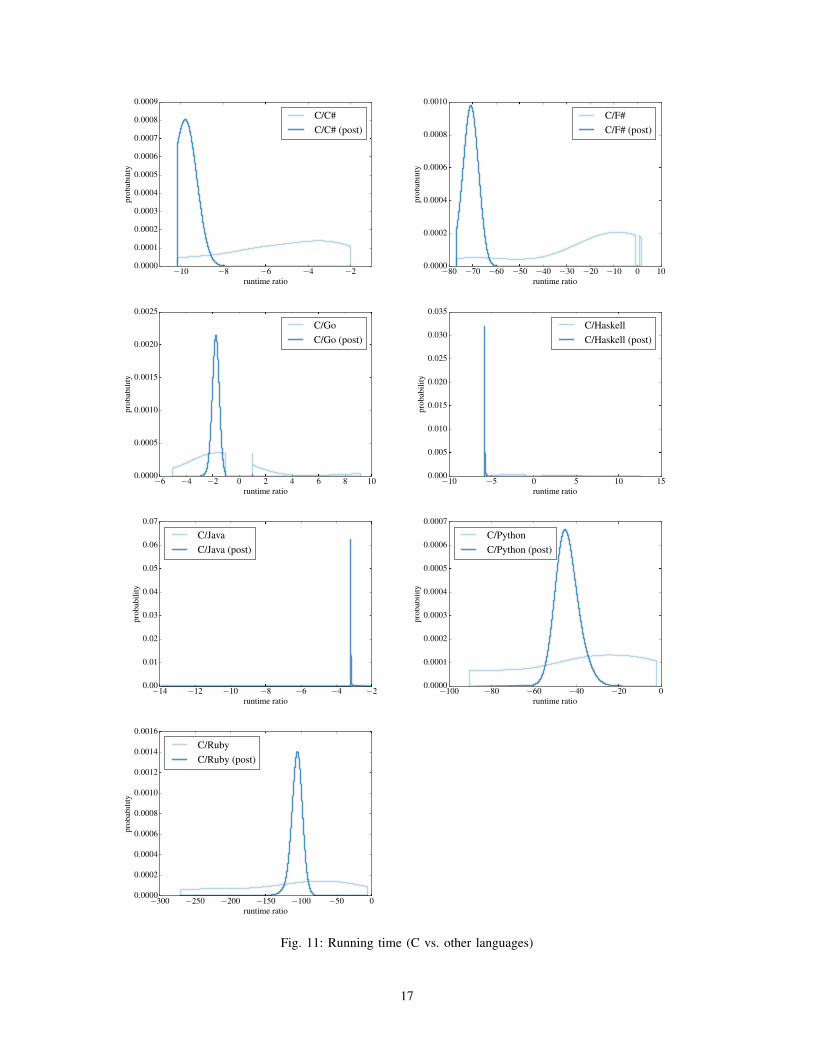
−10 −8 −6 −4 −2runtime ratio

0.0000

0.0001

0.0002

0.0003

0.0004

0.0005

0.0006

0.0007

0.0008

0.0009

prob

abili

tyC/C#C/C# (post)

−80 −70 −60 −50 −40 −30 −20 −10 0 10runtime ratio

0.0000

0.0002

0.0004

0.0006

0.0008

0.0010

prob

abili

ty

C/F#C/F# (post)

−6 −4 −2 0 2 4 6 8 10runtime ratio

0.0000

0.0005

0.0010

0.0015

0.0020

0.0025

prob

abili

ty

C/GoC/Go (post)

−10 −5 0 5 10 15runtime ratio

0.000

0.005

0.010

0.015

0.020

0.025

0.030

0.035

prob

abili

ty

C/HaskellC/Haskell (post)

−14 −12 −10 −8 −6 −4 −2runtime ratio

0.00

0.01

0.02

0.03

0.04

0.05

0.06

0.07

prob

abili

ty

C/JavaC/Java (post)

−100 −80 −60 −40 −20 0runtime ratio

0.0000

0.0001

0.0002

0.0003

0.0004

0.0005

0.0006

0.0007

prob

abili

ty

C/PythonC/Python (post)

−300 −250 −200 −150 −100 −50 0runtime ratio

0.0000

0.0002

0.0004

0.0006

0.0008

0.0010

0.0012

0.0014

0.0016

prob

abili

ty

C/RubyC/Ruby (post)

Fig. 11: Running time (C vs. other languages)

17

−10 −8 −6 −4 −2 0 2 4 6runtime ratio

0.0000

0.0001

0.0002

0.0003

0.0004

0.0005

prob

abili

ty

C#/F#C#/F# (post)

−5 0 5 10 15 20 25 30runtime ratio

0.0000

0.0005

0.0010

0.0015

0.0020

0.0025

0.0030

0.0035

prob

abili

ty

C#/GoC#/Go (post)

0 5 10 15 20 25 30 35 40runtime ratio

0.000

0.005

0.010

0.015

0.020

0.025

prob

abili

ty

C#/HaskellC#/Haskell (post)

−2.0 −1.5 −1.0 −0.5 0.0 0.5 1.0 1.5runtime ratio

0.0000

0.0001

0.0002

0.0003

0.0004

0.0005

0.0006

0.0007

0.0008pr

obab

ility

C#/JavaC#/Java (post)

−30 −25 −20 −15 −10 −5 0 5runtime ratio

0.0000

0.0005

0.0010

0.0015

0.0020

0.0025

0.0030

0.0035

0.0040

0.0045

prob

abili

ty

C#/PythonC#/Python (post)

−50 −40 −30 −20 −10 0runtime ratio

0.0000

0.0001

0.0002

0.0003

0.0004

0.0005

0.0006

0.0007

0.0008

prob

abili

ty

C#/RubyC#/Ruby (post)

Fig. 12: Running time (C# vs. other languages)

18

0 5 10 15 20 25 30 35runtime ratio

0.0000

0.0002

0.0004

0.0006

0.0008

0.0010

0.0012

0.0014

prob

abili

ty

F#/GoF#/Go (post)

0 5 10 15 20 25runtime ratio

0.0000

0.0001

0.0002

0.0003

0.0004

0.0005

0.0006

prob

abili

ty

F#/HaskellF#/Haskell (post)

−4 −2 0 2 4 6 8runtime ratio

0.0000

0.0002

0.0004

0.0006

0.0008

0.0010

prob

abili

ty

F#/JavaF#/Java (post)

−15 −10 −5 0 5 10 15runtime ratio

0.00000

0.00005

0.00010

0.00015

0.00020

0.00025

0.00030

0.00035

0.00040pr

obab

ility

F#/PythonF#/Python (post)

−30 −25 −20 −15 −10 −5 0 5runtime ratio

0.000

0.005

0.010

0.015

0.020

0.025

prob

abili

ty

F#/RubyF#/Ruby (post)

Fig. 13: Running time (F# vs. other languages)

19

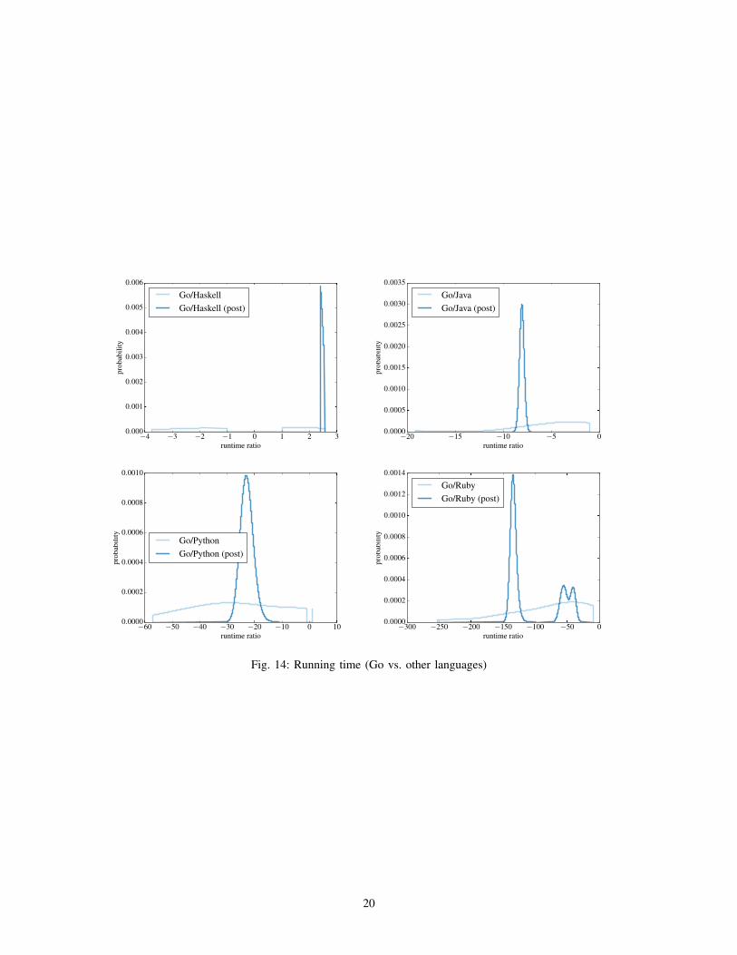
−4 −3 −2 −1 0 1 2 3runtime ratio

0.000

0.001

0.002

0.003

0.004

0.005

0.006

prob

abili

ty

Go/HaskellGo/Haskell (post)

−20 −15 −10 −5 0runtime ratio

0.0000

0.0005

0.0010

0.0015

0.0020

0.0025

0.0030

0.0035

prob

abili

ty

Go/JavaGo/Java (post)

−60 −50 −40 −30 −20 −10 0 10runtime ratio

0.0000

0.0002

0.0004

0.0006

0.0008

0.0010

prob

abili

ty

Go/PythonGo/Python (post)

−300 −250 −200 −150 −100 −50 0runtime ratio

0.0000

0.0002

0.0004

0.0006

0.0008

0.0010

0.0012

0.0014

prob

abili

ty

Go/RubyGo/Ruby (post)

Fig. 14: Running time (Go vs. other languages)

20

−30 −25 −20 −15 −10 −5 0 5runtime ratio

0.000

0.005

0.010

0.015

0.020

0.025pr

obab

ility

Haskell/JavaHaskell/Java (post)

−70 −60 −50 −40 −30 −20 −10 0runtime ratio

0.0000

0.0005

0.0010

0.0015

0.0020

0.0025

prob

abili

ty

Haskell/PythonHaskell/Python (post)

−100 −80 −60 −40 −20runtime ratio

0.000

0.002

0.004

0.006

0.008

0.010

0.012

0.014

prob

abili

ty

Haskell/RubyHaskell/Ruby (post)

Fig. 15: Running time (Haskell vs. other languages)

−30 −25 −20 −15 −10 −5 0 5runtime ratio

0.0000

0.0005

0.0010

0.0015

0.0020

0.0025

prob

abili

ty

Java/PythonJava/Python (post)

−45 −40 −35 −30 −25 −20 −15 −10 −5 0runtime ratio

0.0000

0.0001

0.0002

0.0003

0.0004

0.0005

0.0006

0.0007

0.0008

prob

abili

ty

Java/RubyJava/Ruby (post)

Fig. 16: Running time (Java vs. other languages)

21

−40 −35 −30 −25 −20 −15 −10 −5 0 5runtime ratio

0.0000

0.0002

0.0004

0.0006

0.0008

0.0010

0.0012

prob

abili

ty

Python/RubyPython/Ruby (post)

Fig. 17: Running time (Python vs. other languages)

22

CGoC#

F#

Python

Ruby

JavaHaskell

(a) Previous analysis [43].

CC#F#Go

Haskell

Java

Python

Ruby

(b) Bayesian analysis.

Fig. 18: Comparison of used memory: qualitative summaries.

2) Memory usage: Rosetta’s memory experiments measure the maximum RAM usage of programs implementing the sametasks: M(`, t) is the maximum RAM used by the best (that is, using the least amount of memory) implementation of t in language`; and M(`1, `2) is the vector of elementwise ratios (4), defined like S(`1, `2) but with respect to M(`1) and M(`2). Bench alsoincludes memory experiments that determine vectors M(`1, `2) and sets M∆(`1, `2, t), defined just like their counterparts forrunning time but measuring the maximum RAM used in each case. The following graphs, tables, and plots are the counterpartof the analysis of running time S with respect to the data M on memory usage.

LANGUAGE MEASURE C C# F# Go Haskell Java PythonC# CI (-12.9, 9.6)

m 9.83µ 1.67

F# CI (-65.3, -22.1) (-9.2, -1.4)m -35.28 -6.32µ -39.51 -5.19

Go CI (-3.2, -1.9) (-7.0, 8.8) (61.6, 63.2)m -1.84 -2.96 62.74µ -2.39 0.68 62.72

Haskell CI (-12.8, -8.5) (-5.0, -1.0) (46.1, 49.3) (-3.6, -3.4)m -11.11 -4.14 48.76 -3.56µ -10.71 -2.74 48.05 -3.56

Java CI (-7.8, 1.7) (-4.2, -1.2) (1.4, 4.1) (-33.5, -31.8) (-2.7, 1.2)m -1.06 -2.34 2.26 -32.9 -2.07µ -3.4 -2.52 2.3 -32.89 -1.44

Python CI (-18.0, -2.1) (-15.5, 24.8) (-4.3, 7.1) (-7.0, -1.5) (-2.2, 4.6) (-10.6, -1.6)m -11.1 -7.58 -2.62 -6.82 2.35 -3.51µ -9.73 0.68 1.83 -4.49 2.23 -5.73

Ruby CI (-229.5, -157.0) (-36.5, -6.2) (-23.6, -2.9) (-194.8, -174.3) (-60.7, -10.6) (-25.6, -5.3) (-12.2, -4.3)m -154.78 -15.95 -18.33 -190.44 -43.66 -13 -10.82µ -195.45 -17.16 -9.92 -184.58 -35.02 -12.07 -7.18

TABLE 19: Comparison of maximum RAM usage

C

C#

F#

Go

HaskellJava

Python

Ruby

Fig. 20: Maximum RAM usage

23

−50 −40 −30 −20 −10 0 10 20memory ratio

0.00000

0.00005

0.00010

0.00015

0.00020

0.00025

0.00030

0.00035

0.00040

0.00045

prob

abili

tyC/C#C/C# (post)

−80 −70 −60 −50 −40 −30 −20 −10 0memory ratio

0.00000

0.00005

0.00010

0.00015

0.00020

0.00025

0.00030

0.00035

0.00040

prob

abili

ty

C/F#C/F# (post)

−12 −10 −8 −6 −4 −2 0 2memory ratio

0.0000

0.0002

0.0004

0.0006

0.0008

0.0010

0.0012

0.0014

prob

abili

ty

C/GoC/Go (post)

−80 −70 −60 −50 −40 −30 −20 −10 0memory ratio

0.0000

0.0005

0.0010

0.0015

0.0020

0.0025

0.0030

prob

abili

ty

C/HaskellC/Haskell (post)

−50 −40 −30 −20 −10 0 10 20memory ratio

0.0000

0.0002

0.0004

0.0006

0.0008

0.0010

0.0012

prob

abili

ty

C/JavaC/Java (post)

−20 −15 −10 −5 0memory ratio

0.00000

0.00002

0.00004

0.00006

0.00008

0.00010

0.00012

0.00014

0.00016

prob

abili

ty

C/PythonC/Python (post)

−1000 −800 −600 −400 −200 0memory ratio

0.0000

0.0005

0.0010

0.0015

0.0020

0.0025

prob

abili

ty

C/RubyC/Ruby (post)

Fig. 21: Maximum RAM usage (C vs. other languages)

24

−100 −80 −60 −40 −20 0 20memory ratio

0.0000

0.0005

0.0010

0.0015

0.0020

prob

abili

ty

C#/F#C#/F# (post)

−40 −30 −20 −10 0 10 20 30memory ratio

0.0000

0.0001

0.0002

0.0003

0.0004

0.0005

0.0006

0.0007

0.0008

0.0009

prob

abili

ty

C#/GoC#/Go (post)

−40 −30 −20 −10 0 10 20 30 40memory ratio

0.0000

0.0005

0.0010

0.0015

0.0020

0.0025

prob

abili

ty

C#/HaskellC#/Haskell (post)

−60 −50 −40 −30 −20 −10 0 10memory ratio

0.0000

0.0005

0.0010

0.0015

0.0020

0.0025pr

obab

ility

C#/JavaC#/Java (post)

−120 −100 −80 −60 −40 −20 0 20 40memory ratio

0.0000

0.0002

0.0004

0.0006

0.0008

0.0010

0.0012

0.0014

prob

abili

ty

C#/PythonC#/Python (post)

−900 −800 −700 −600 −500 −400 −300 −200 −100 0memory ratio

0.0000

0.0005

0.0010

0.0015

0.0020

0.0025

0.0030

0.0035

0.0040

0.0045

prob

abili

ty

C#/RubyC#/Ruby (post)

Fig. 22: Maximum RAM usage (C# vs. other languages)

25

0 10 20 30 40 50 60 70memory ratio

0.000

0.002

0.004

0.006

0.008

0.010

0.012

0.014

prob

abili

ty

F#/GoF#/Go (post)

0 10 20 30 40 50memory ratio

0.0000

0.0005

0.0010

0.0015

0.0020

0.0025

prob

abili

ty

F#/HaskellF#/Haskell (post)

0 10 20 30 40 50 60memory ratio

0.0000

0.0005

0.0010

0.0015

0.0020

0.0025

0.0030

0.0035

0.0040

prob

abili

ty

F#/JavaF#/Java (post)

−60 −40 −20 0 20 40 60memory ratio

0.0000

0.0005

0.0010

0.0015

0.0020pr

obab

ility

F#/PythonF#/Python (post)

−600 −500 −400 −300 −200 −100 0memory ratio

0.000

0.001

0.002

0.003

0.004

0.005

0.006

prob

abili

ty

F#/RubyF#/Ruby (post)

Fig. 23: Maximum RAM usage (F# vs. other languages)

26

−4 −3 −2 −1 0 1 2memory ratio

0.000

0.002

0.004

0.006

0.008

0.010

prob

abili

ty

Go/HaskellGo/Haskell (post)

−35 −30 −25 −20 −15 −10 −5 0 5 10memory ratio

0.0000

0.0005

0.0010

0.0015

0.0020

0.0025

0.0030

0.0035

0.0040

0.0045

prob

abili

ty

Go/JavaGo/Java (post)

−8 −7 −6 −5 −4 −3 −2 −1memory ratio

0.00000

0.00002

0.00004

0.00006

0.00008

0.00010

0.00012

0.00014

0.00016

prob

abili

ty

Go/PythonGo/Python (post)

−700 −600 −500 −400 −300 −200 −100 0memory ratio

0.000

0.001

0.002

0.003

0.004

0.005

prob

abili

ty

Go/RubyGo/Ruby (post)

Fig. 24: Maximum RAM usage (Go vs. other languages)

27

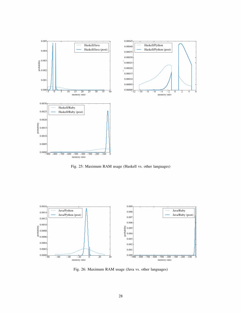
−5 0 5 10 15 20 25 30 35 40memory ratio

0.000

0.001

0.002

0.003

0.004

0.005pr

obab

ility

Haskell/JavaHaskell/Java (post)

−12 −10 −8 −6 −4 −2 0 2 4 6memory ratio

0.00000

0.00005

0.00010

0.00015

0.00020

0.00025

0.00030

0.00035

0.00040

0.00045

prob

abili

ty

Haskell/PythonHaskell/Python (post)

−900 −800 −700 −600 −500 −400 −300 −200 −100 0memory ratio

0.0000

0.0005

0.0010

0.0015

0.0020

0.0025

0.0030

prob

abili

ty

Haskell/RubyHaskell/Ruby (post)

Fig. 25: Maximum RAM usage (Haskell vs. other languages)

−80 −60 −40 −20 0 20 40memory ratio

0.0000

0.0002

0.0004

0.0006

0.0008

0.0010

0.0012

0.0014

0.0016

prob

abili

ty

Java/PythonJava/Python (post)

−900 −800 −700 −600 −500 −400 −300 −200 −100 0memory ratio

0.000

0.001

0.002

0.003

0.004

0.005

0.006

0.007

0.008

0.009

prob

abili

ty

Java/RubyJava/Ruby (post)

Fig. 26: Maximum RAM usage (Java vs. other languages)

28

−160 −140 −120 −100 −80 −60 −40 −20 0memory ratio

0.0000

0.0005

0.0010

0.0015

0.0020

0.0025

0.0030

prob

abili

ty

Python/RubyPython/Ruby (post)

Fig. 27: Maximum RAM usage (Python vs. other languages)

29

B. Agile vs. Structured Study

1) Success: Tab. 28 shows the distributions oC for the nine combinations of process categories we analyze: A, AIL, AILT ,AIT , AL, ALT , AT , AT , IT , and T . These are used as baseline distributions in computing the Bayes factors. Tab. 28 is likeTab. 1 in the main paper.

Tab. 29 shows the Bayes factors KC(D) from AvsS, for each choice of baseline distribution C in Tab. 28. Each row usesdifferent weights wps for the likelihoods (2) and (3). The table is partitioned in four parts separated by horizontal lines; theycorrespond, from top to bottom, to the analysis using different choices of lower bound b = 1,3,4,5 for the scaling of data(row header). The scaling of data translates a project outcome 1≤ x≤ 10 into an outcome 0≤ x′ ≤ r using lower bound b asfollows. For 0 ≤ k ≤ r, let σr(k) = b+ k(10−b)/r be a uniformly spaced point over [b,10]; then x′ = argmink |σr(k)− x|. Inthe main paper, Tab. 2 shows the data for b = 1.

A AIL AILT AIT AL ALT AT IT ToC[0] 7 % 8 % 10 % 11 % 7 % 11 % 12 % 12 % 18 %oC[1] 30 % 27 % 28 % 29 % 27 % 29 % 31 % 29 % 32 %oC[2] 63 % 65 % 62 % 60 % 66 % 60 % 57 % 59 % 50 %

TABLE 28: Different distributions for the baseline probability of outcome for software projects: for C one of the subsets of{A, I,L,T} in the column headers, oC[k] is the probability that outcome is k ∈ {0,1,2} in processes of category C.

A AIL AILT AIT AL ALT AT IT Tuniform 0.2456 0.2609 0.1655 0.1362 0.2881 0.1228 0.0780 0.0986 0.0131triangle 0.2472 0.2614 0.1704 0.1411 0.2883 0.1284 0.0827 0.1037 0.0151power 0.2484 0.2618 0.1735 0.1441 0.2885 0.1320 0.0855 0.1069 0.0162exp 0.2525 0.2633 0.1860 0.1567 0.2891 0.1471 0.0986 0.1208 0.0229uniform 0.0329 0.0277 0.0625 0.0735 0.0188 0.0782 0.0888 0.0853 0.0424triangle 0.0348 0.0295 0.0648 0.0760 0.0201 0.0807 0.0915 0.0879 0.0460power 0.0361 0.0307 0.0665 0.0777 0.0210 0.0824 0.0933 0.0897 0.0480exp 0.0414 0.0358 0.0726 0.0843 0.0248 0.0888 0.1003 0.0965 0.0583uniform 0.0406 0.0336 0.0854 0.1055 0.0220 0.1151 0.1461 0.1325 0.1102triangle 0.0427 0.0356 0.0877 0.1077 0.0235 0.1170 0.1478 0.1344 0.1156power 0.0442 0.0370 0.0894 0.1094 0.0245 0.1185 0.1491 0.1358 0.1187exp 0.0501 0.0427 0.0953 0.1152 0.0287 0.1235 0.1537 0.1406 0.1330uniform 0.0406 0.0336 0.0854 0.1055 0.0220 0.1151 0.1461 0.1325 0.1102triangle 0.0427 0.0356 0.0877 0.1077 0.0235 0.1170 0.1478 0.1344 0.1156power 0.0442 0.0370 0.0894 0.1094 0.0245 0.1185 0.1491 0.1358 0.1187exp 0.0501 0.0427 0.0953 0.1152 0.0287 0.1235 0.1537 0.1406 0.1330

TABLE 29: Bayes factors K estimating to what extent the hypothesis “agile leads to more successful projects” is supportedover the other hypothesis “agile is no better than structured”.

2) Importance for customers: The data in AvsS also reports, for each project p ∈ P, its importance for customers I(p) on ascale 1–10, where 1 denotes an unimportant project and 10 denotes a very critical one. The multisets IA, IS, and I are definedsimilarly to OA, OS, and O but for importance assessments.

The data in ITP also assesses “stakeholder value”, which we can assimilate to importance for customers—a most significantgroup of stakeholders. For each category c∈ {A,H, I,L,T}, each respondent r ∈ R assesses the projects in category c accordingto their stakeholder value vc(r) on a scale 0–4, where 0 denotes no value and 4 denotes very high value.19 For every non-emptysubset C ⊆ {A,H, I,L,T}, we define a distribution ιC over values in the range [0..4] as follows. If C is a singleton set {c}with c ∈ {A,H, I,L,T}, ιc[k] is the probability |{r ∈ R | vc(r) = k}|/|R| that a project in category c has value k. If C is anynon-empty subset of {A,H, I,L,T}, ιC[k] is the weighted average ιC[k] = ∑c∈C ιc[k]/|C|. Tab. 30 shows the distributions ιC forthe nine combinations of process categories we analyze.

A AIL AILT AIT AL ALT AT IT TιC[0] 0 % 1 % 2 % 2 % 0 % 3 % 3 % 3 % 7 %ιC[1] 4 % 3 % 9 % 9 % 6 % 14 % 15 % 11 % 26 %ιC[2] 15 % 18 % 20 % 21 % 13 % 19 % 21 % 24 % 28 %ιC[3] 30 % 35 % 35 % 35 % 33 % 34 % 32 % 37 % 35 %ιC[4] 51 % 43 % 34 % 33 % 48 % 30 % 29 % 25 % 4 %

TABLE 30: Different distributions for the baseline probability of customer importance for software projects: for C one of thesubsets of {A, I,L,T} in the column headers, ιC[k] is the probability that customer importance is k ∈ {0,1,2} in processes ofcategory C.

19Respondents could also mark this question as “not applicable”, in which case we ignored their answer.

30

The Bayes factors are computed just like the analysis of success mutatis mutandis. Tab. 2 shows the Bayes factors for thedata IA ∪ IS from AvsS, using the same conventions as Tab. 29 and using ιC as baseline distributions, for C one of the ninedistributions in Tab. 30.

A AIL AILT AIT AL ALT AT IT Tuniform 0.0395 0.0494 0.0087 0.0087 0.0395 0.0038 0.0019 0.0019 0.0000triangle 0.0429 0.0549 0.0114 0.0116 0.0435 0.0057 0.0029 0.0030 0.0000power 0.0449 0.0570 0.0118 0.0121 0.0452 0.0058 0.0029 0.0030 0.0000exp 0.0547 0.0728 0.0217 0.0238 0.0566 0.0140 0.0074 0.0078 0.0001uniform 0.0003 0.0152 0.0800 0.0800 0.0003 0.0418 0.0205 0.0205 0.0001triangle 0.0003 0.0162 0.0839 0.0854 0.0003 0.0477 0.0238 0.0241 0.0002power 0.0004 0.0168 0.0855 0.0877 0.0004 0.0499 0.0248 0.0252 0.0001exp 0.0005 0.0196 0.0954 0.1024 0.0004 0.0679 0.0348 0.0365 0.0007uniform 0.0000 0.0000 0.0002 0.0002 0.0000 0.0053 0.0129 0.0129 0.0001triangle 0.0000 0.0000 0.0003 0.0003 0.0000 0.0063 0.0154 0.0155 0.0002power 0.0000 0.0000 0.0003 0.0003 0.0000 0.0067 0.0163 0.0164 0.0001exp 0.0000 0.0000 0.0004 0.0004 0.0000 0.0099 0.0242 0.0250 0.0007uniform 0.0000 0.0000 0.0010 0.0010 0.0000 0.0035 0.0203 0.0203 0.0007triangle 0.0000 0.0000 0.0012 0.0012 0.0000 0.0040 0.0231 0.0232 0.0011power 0.0000 0.0000 0.0014 0.0013 0.0000 0.0042 0.0247 0.0247 0.0011exp 0.0000 0.0000 0.0021 0.0020 0.0000 0.0057 0.0330 0.0331 0.0037

TABLE 31: Bayes factors K estimating to what extent the hypothesis “agile is used for projects that are more important forcustomers” is supported over the other hypothesis “agile is no better than structured”.

31

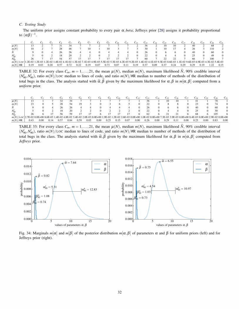
C. Testing Study

The uniform prior assigns constant probability to every pair α,beta; Jeffreys prior [28] assigns it probability proportionalto (αβ )−1.

C1 C2 C3 C4 C5 C6 C7 C8 C9 C10 C11 C12 C13 C14 C15 C16 C17 C18 C19 C20 C21µ(N) 13 2 7 31 34 7 7 2 7 7 7 2 36 2 10 10 2 40 2 68 2m(N) 10 2 7 28 46 7 10 1 10 3 7 3 30 1 10 17 4 26 3 110 2N̂ 9 0 4 26 26 4 4 0 4 4 4 0 26 0 6 6 0 40 0 60 0N l

90 5 0 2 18 20 2 2 0 2 2 2 0 22 0 4 4 0 25 0 49 0Nh

90 26 7 17 54 57 17 17 7 17 17 17 7 60 7 22 22 7 66 7 100 7m(N)/LOC 1.2E-02 1.2E-03 1.2E-02 1.4E-02 4.1E-02 1.3E-02 7.1E-03 4.9E-03 5.5E-02 5.3E-03 4.2E-03 9.2E-03 1.4E-02 4.1E-03 9.3E-03 8.6E-03 1.1E-02 9.6E-03 6.9E-03 4.3E-02 5.4E-03m(N)/#R 0.19 0.03 0.20 0.57 0.72 0.22 0.19 0.07 0.73 0.07 0.11 0.19 0.37 0.09 0.37 0.24 0.29 0.29 0.19 1.22 0.15

TABLE 32: For every class Cm, m = 1, . . . ,21, the mean µ(N), median m(N), maximum likelihood N̂, 90% credible interval(Nl

90,Nl90), ratio m(N)/LOC median to lines of code, and ratio m(N)/#R median to number of methods of the distribution of

total bugs in the class. The analysis started with α̂, β̂ given by the maximum likelihood for α,β in m[α,β ] computed from auniform prior.

C1 C2 C3 C4 C5 C6 C7 C8 C9 C10 C11 C12 C13 C14 C15 C16 C17 C18 C19 C20 C21µ(N) 13 1 7 32 34 7 7 1 7 7 7 1 36 1 10 10 1 41 1 70 1m(N) 23 0 5 28 54 19 3 0 3 6 5 0 22 0 8 8 0 23 0 74 0N̂ 9 0 4 26 26 4 4 0 4 4 4 0 26 0 6 6 0 40 0 60 0N l

90 5 0 2 18 20 2 2 0 2 2 2 0 22 0 4 4 0 25 0 50 0Nh

90 26 6 17 56 59 17 17 6 17 17 17 6 62 6 21 21 6 68 6 105 6m(N)/LOC 2.7E-02 0.0E+00 8.6E-03 1.4E-02 4.8E-02 3.4E-02 2.0E-03 0.0E+00 1.9E-02 1.2E-02 2.6E-03 0.0E+00 1.0E-02 0.0E+00 7.3E-03 3.9E-03 0.0E+00 8.4E-03 0.0E+00 2.9E-02 0.0E+00m(N)/#R 0.43 0.00 0.14 0.57 0.84 0.59 0.05 0.00 0.25 0.15 0.07 0.00 0.26 0.00 0.29 0.11 0.00 0.25 0.00 0.83 0.00

TABLE 33: For every class Cm, m = 1, . . . ,21, the mean µ(N), median m(N), maximum likelihood N̂, 90% credible interval(Nl

90,Nl90), ratio m(N)/LOC median to lines of code, and ratio m(N)/#R median to number of methods of the distribution of

total bugs in the class. The analysis started with α̂, β̂ given by the maximum likelihood for α,β in m[α,β ] computed fromJeffreys prior.

0 5 10 15 20values of parameters α,β

0.000

0.002

0.004

0.006

0.008

0.010

0.012

0.014

0.016

prob

abili

ty

α̂ = 7.64

αh90 = 12.83

α l90 = 5.31

β̂ = 0.82

β h90 = 1.08

β l90 = 0.74

α

β

0 5 10 15 20values of parameters α,β

0.000

0.002

0.004

0.006

0.008

0.010

0.012

0.014

0.016

0.018

prob

abili

ty

α̂ = 6.55

αh90 = 10.97

α l90 = 4.54

β̂ = 0.75

β h90 = 1.03

β l90 = 0.73

α

β

Fig. 34: Marginals m[α] and m[β ] of the posterior distribution m[α,β ] of parameters α and β for uniform priors (left) and forJeffreys prior (right).

32

0 20 40 60 80 100 120 140 160# bugs

0.0

0.2

0.4

0.6

0.8

1.0

prob

abili

ty/f

ract

ion

α l90,β

l90

α̂, β̂

αh90,β

h90

0 20 40 60 80 100 120 140 160# bugs

0.0

0.2

0.4

0.6

0.8

1.0

prob

abili

ty/f

ract

ion

α l90,β

l90

α̂, β̂

αh90,β

h90

Fig. 35: Cumulative distribution function Wα,β for the values of α and β in Fig. 34 for uniform priors (left) and for Jeffreysprior (right).

0 2 4 6 8 10 12 14values of α,β within 90% credible intervals

0.000

0.002

0.004

0.006

0.008

0.010

0.012

0.014

0.016

prob

abili

tyof

atm

ost0

erro

rs

α

β

0 2 4 6 8 10 12values of α,β within 90% credible intervals

0.000

0.002

0.004

0.006

0.008

0.010

0.012

0.014

prob

abili

tyof

atm

ost0

erro

rs

α

β

Fig. 36: Marginals of the probability distribution for a module having zero bugs detected by random testing with strongspecifications for the values of α and β in a 90% credible interval for uniform priors (left) and for Jeffreys prior (right).

33

0 2 4 6 8 10 12 14values of α,β within 90% credible intervals

0.000

0.002

0.004

0.006

0.008

0.010

0.012

0.014

prob

abili

tyof

atm

ost5

erro

rs

α

β

0 2 4 6 8 10 12values of α,β within 90% credible intervals

0.000

0.002

0.004

0.006

0.008

0.010

0.012

0.014

prob

abili

tyof

atm

ost5

erro

rsα

β

Fig. 37: Marginals of the probability distribution for a module having at most five bugs detected by random testing with strongspecifications for the values of α and β in a 90% credible interval for uniform priors (left) and for Jeffreys prior (right).

34

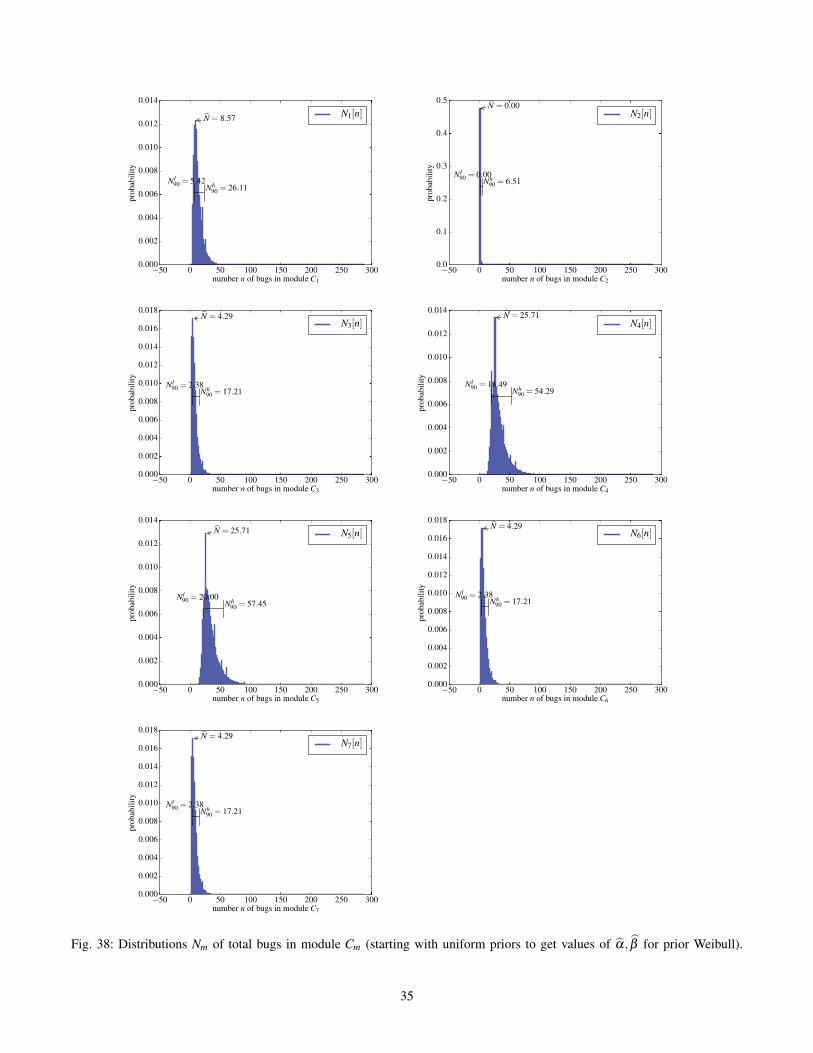
−50 0 50 100 150 200 250 300number n of bugs in module C1

0.000

0.002

0.004

0.006

0.008

0.010

0.012

0.014

prob

abili

ty

N̂ = 8.57

Nh90 = 26.11

Nl90 = 5.42

N1[n]

−50 0 50 100 150 200 250 300number n of bugs in module C2

0.0

0.1

0.2

0.3

0.4

0.5

prob

abili

ty

N̂ = 0.00

Nh90 = 6.51

Nl90 = 0.00

N2[n]

−50 0 50 100 150 200 250 300number n of bugs in module C3

0.000

0.002

0.004

0.006

0.008

0.010

0.012

0.014

0.016

0.018

prob

abili

ty

N̂ = 4.29

Nh90 = 17.21

Nl90 = 2.38

N3[n]

−50 0 50 100 150 200 250 300number n of bugs in module C4

0.000

0.002

0.004

0.006

0.008

0.010

0.012

0.014

prob

abili

ty

N̂ = 25.71

Nh90 = 54.29

Nl90 = 18.49

N4[n]

−50 0 50 100 150 200 250 300number n of bugs in module C5

0.000

0.002

0.004

0.006

0.008

0.010

0.012

0.014

prob

abili

ty

N̂ = 25.71

Nh90 = 57.45

Nl90 = 20.00

N5[n]

−50 0 50 100 150 200 250 300number n of bugs in module C6

0.000

0.002

0.004

0.006

0.008

0.010

0.012

0.014

0.016

0.018

prob

abili

ty

N̂ = 4.29

Nh90 = 17.21

Nl90 = 2.38

N6[n]

−50 0 50 100 150 200 250 300number n of bugs in module C7

0.000

0.002

0.004

0.006

0.008

0.010

0.012

0.014

0.016

0.018

prob

abili

ty

N̂ = 4.29

Nh90 = 17.21

Nl90 = 2.38

N7[n]

Fig. 38: Distributions Nm of total bugs in module Cm (starting with uniform priors to get values of α̂, β̂ for prior Weibull).

35

−50 0 50 100 150 200 250 300number n of bugs in module C8

0.0

0.1

0.2

0.3

0.4

0.5

prob

abili

ty

N̂ = 0.00

Nh90 = 6.51

Nl90 = 0.00

N8[n]

−50 0 50 100 150 200 250 300number n of bugs in module C9

0.000

0.002

0.004

0.006

0.008

0.010

0.012

0.014

0.016

0.018

prob

abili

ty

N̂ = 4.29

Nh90 = 17.21

Nl90 = 2.38

N9[n]

−50 0 50 100 150 200 250 300number n of bugs in module C10

0.000

0.002

0.004

0.006

0.008

0.010

0.012

0.014

0.016

0.018

prob

abili

ty

N̂ = 4.29

Nh90 = 17.21

Nl90 = 2.38

N10[n]

−50 0 50 100 150 200 250 300number n of bugs in module C11

0.000

0.002

0.004

0.006

0.008

0.010

0.012

0.014

0.016

0.018

prob

abili

ty

N̂ = 4.29

Nh90 = 17.21

Nl90 = 2.38

N11[n]

−50 0 50 100 150 200 250 300number n of bugs in module C12

0.0

0.1

0.2

0.3

0.4

0.5

prob

abili

ty

N̂ = 0.00

Nh90 = 6.51

Nl90 = 0.00

N12[n]

−50 0 50 100 150 200 250 300number n of bugs in module C13

0.000

0.002

0.004

0.006

0.008

0.010

0.012

prob

abili

ty

N̂ = 25.71

Nh90 = 60.37

Nl90 = 21.70

N13[n]

−50 0 50 100 150 200 250 300number n of bugs in module C14

0.0

0.1

0.2

0.3

0.4

0.5

prob

abili

ty

N̂ = 0.00

Nh90 = 6.51

Nl90 = 0.00

N14[n]

Fig. 39: Distributions Nm of total bugs in module Cm (starting with uniform priors to get values of α̂, β̂ for prior Weibull).

36

−50 0 50 100 150 200 250 300number n of bugs in module C15

0.000

0.002

0.004

0.006

0.008

0.010

0.012

0.014

prob

abili

ty

N̂ = 5.71

Nh90 = 21.70

Nl90 = 3.97

N15[n]

−50 0 50 100 150 200 250 300number n of bugs in module C16

0.000

0.002

0.004

0.006

0.008

0.010

0.012

0.014

prob

abili

ty

N̂ = 5.71

Nh90 = 21.70

Nl90 = 3.97

N16[n]

−50 0 50 100 150 200 250 300number n of bugs in module C17

0.0

0.1

0.2

0.3

0.4

0.5

prob

abili

ty

N̂ = 0.00

Nh90 = 6.51

Nl90 = 0.00

N17[n]

−50 0 50 100 150 200 250 300number n of bugs in module C18

0.000

0.001

0.002

0.003

0.004

0.005

0.006

0.007

0.008

0.009

prob

abili

ty

N̂ = 40.00

Nh90 = 65.77

Nl90 = 25.15

N18[n]

−50 0 50 100 150 200 250 300number n of bugs in module C19

0.0

0.1

0.2

0.3

0.4

0.5

prob

abili

ty

N̂ = 0.00

Nh90 = 6.51

Nl90 = 0.00

N19[n]

−50 0 50 100 150 200 250 300number n of bugs in module C20

0.000

0.002

0.004

0.006

0.008

0.010

0.012

0.014

0.016

prob

abili

ty

N̂ = 60.00

Nh90 = 99.57

Nl90 = 49.47

N20[n]

−50 0 50 100 150 200 250 300number n of bugs in module C21

0.0

0.1

0.2

0.3

0.4

0.5

prob

abili

ty

N̂ = 0.00

Nh90 = 6.51

Nl90 = 0.00

N21[n]

Fig. 40: Distributions Nm of total bugs in module Cm (starting with uniform priors to get values of α̂, β̂ for prior Weibull).

37