Bayesian Sensor Fusion Methods for Dynamic Object Tracking—A Comparative Study · ·...

Ivan Markovic, Ivan Petrovic

Bayesian Sensor Fusion Methods for Dynamic ObjectTracking — A Comparative Study

In this paper we study the problem of Bayesian sensor fusion for dynamic object tracking. The prospectsof utilizing measurements from several sensors to infer about a system state are manyfold and they range fromincreased estimate accuracy to more reliable and robust estimates. Sensor measurements may be combined, orfused, at a variety of levels; from the raw data level to a state vector level, or at the decision level. In this paper wemainly focus on the Bayesian fusion at the likelihood and state vector level. We analyze two groups of data fusionmethods: centralized independent likelihood fusion, where the sensors report only its measurement to the fusioncenter, and hierarchical fusion, where each sensor runs its own local estimate which is then communicated to thefusion center along with the corresponding uncertainty. We compare the prospects of utilizing both approaches, andpresent explicit solutions in the forms of extended information filter, unscented information filter, and particle filter.Furthermore, we also propose a solution for fusion of arbitrary filters and test it on a hierarchical fusion example oftwo of the aforementioned filters. Hence, the main contributions of this paper are systematic comparative study ofBayesian fusion methods, and a method for hierarchical fusion of arbitrary filters. The fusion methods are testedon a synthetic data generated by multiple Monte Carlo runs for tracking of a dynamic object with several sensorsof different accuracies by analyzing the quadratic Rényi entropy and root-mean-square error.

Key words: Bayesian sensor fusion, Information filter, Particle filter, Rényi entropy

Komparativna studija Bayesovih metoda fuzije u svrhu pracenja gibajucih objekata. U ovom clankurazmatra se problem Bayesove fuzije senzora u svrhu pracenja gibajucih objekata. Prednosti korištenja mjerenjaviše senzora kako bi se estimiralo stanje sustava su višestruke te se krecu od povecanja preciznosti do pouzdanijihi robusnijih estimacija. Fuzija mjerenja senzora može se izvršiti na razini neobradenih mjerenja, razini estimacijestanja te na još višoj razini–razini donošenja odluka. U ovom se clanku fokusira na Bayesovu fuziju senzora narazini funkcija vjerodostojnosti i na razini vektora stanja sustava. Analiziramo dvije grupe metoda fuzije podataka:centraliziranu fuziju nezavisnih funkcija vjerodostojnosti, u kojoj senzori šalju samo svoja mjerenja centru fuzije,i hijerarhijsku fuziju, gdje svaki senzor lokalno estimira stanje sustava koje se potom šalje centru fuzije zajedno sapripadajucom nesigurnosti. Usporedujemo prednosti korištenja oba pristupa te predstavljamo eksplicitna rješenjau obliku proširenog informacijskog filtra, nederivacijskog informacijskog filtra te cesticnog filtra. Nadalje, takoderse predlaže rješenje za fuziju proizvoljnih filtara te se testira na primjeru hijerarhijske fuzije dvaju razlicitih tipovafiltara. Glavni doprinos ovoga clanka je u sustavnoj komparativnoj studiji Bayesovih metoda fuzije te u metodiza hijerarhijsku fuziju proizvoljnih filtara. Metode fuzije provjerene su na, iz višestrukih Monte Carlo simulacijadobivenom, sintetickom skupu podataka pracenja gibajuceg objekta s više senzora razlicitih preciznosti analizirajucikvadraticnu Rényijevu entropiju i srednju kvadraticnu pogrešku.

Kljucne rijeci: Bayesova fuzija senzora, informacijski filtar, cesticni filtar, Rényijeva entropija

1 INTRODUCTIONThe prospects of utilizing measurements from several

sensors to infer about a system state are manyfold. To be-gin with, the use of multiple sensors results in increasedsensor measurement accuracy, and moreover, additionalsensors will never reduce the performance of the optimalestimator [1]. However, in order to ensure this perfor-

mance, special care must be taken when choosing the pro-cess model [2]. Furthermore, system reliability increaseswith additional sensors, since the system itself becomesmore resilient to sensor failure [3]. Therefore, by com-bining data from multiple sensors, and perhaps related in-formation from associated databases, we can achieve im-proved accuracies and more specific inferences than using

Bayesian Sensor Fusion Methods for Dynamic Object Tracking — A Comparative Study I. Markovic, I. Petrovic

only a single sensor [4].

Sensor measurements may be combined, or fused, ata variety of levels; from the raw data level to a state vec-tor level, or at the decision level [4]. Raw sensor data canbe directly combined if the sensor data are commensurate(i.e., if the sensors are measuring the same physical phe-nomena), while if the sensor data are noncommensurate,then the sensor data, i.e. sensor information, must be fusedat a feature/state vector level or decision level.

Information from multiple sensors can be classified asredundant or complementary [3]. Redundant informationis provided from multiple sensors (or a single sensor overtime) when each sensor perceives the same feature in theenvironment. On the other hand, complementary informa-tion from multiple sensors enables the system to perceivefeatures impossible to perceive by using just a single sen-sor. But what is in common for both classifications, is thatall the sensors are used to somehow infer about a systemstate. It is important to note that complementary sensors donot have to necessarily provide information about the fullsystem state. Some sensors, like omnidrectional camerasand microphone arrays, measure angle and not the range ofthe detected objects, while laser range scanners and depthcameras can give measurements in 2D or 3D. Moreover,some sensors can provide measurements at higher ratesthan others, thus making sensor fusion an even more chal-lenging problem.

One way of approaching the problem of sensor fusionis at the likelihood level. Basically, each sensor measure-ment is modelled as a Gaussian random variable and theresulting fused distribution is also Gaussian with the newfused mean and covariance. In [5], the fused moments arecalculated by optimizing a weighted sum of Gaussian ran-dom variables so as to minimise the volume of the fuseduncertainty ellipsoid. The resulting moments are equalto as if they were obtained by calculating the product ofGaussian distributions. Similar results were obtained in [6]where the fused moments are calculated by estimating themoments of a product of Gaussians via maximum likeli-hood approach. Both of these methods do not take anypast measurements into account, and if tracking is neededthen a different approach needs to be utilised.

If the system is linear and the system state is modeledas Gaussian, then multisensor fusion can be performedwith the decentralized Kalman filter (DKF) proposed in[7]. The DKF enables us to fuse not only the measure-ments, but also the local independent Kalman filters. Theinverse covariance form is utilized, thus resulting in addi-tive fusion equations, which can further be elegantly trans-lated to the information filter form as shown in [8]. Forthe case of non-linear systems the extended information fil-ter (EIF) or the unscented information filter (UIF) [9] can

be utilised. Another approach, proposed in [10], is to de-fine for each sensor system, a separate and specific Gaus-sian probability distribution and to fuse them using covari-ance intersection method [11]. If the underlying distribu-tion characterizing the system is not Gaussian and possiblynon-linear, then usually particle filters (PF) are utilized.In [12] a distributed particle filtering algorithm is proposedwhere each sensor maintains a particle filter and the in-formation is propagated in a sensor network in the formof partial likelihood functions. The last sensor then back-propagates the final importance distribution so that a newset of particles is generated at each sensor using the finaldistribution. The standard particle filter algorithm was de-centralized in [13] by communicating and fusing only themost informative subsets of samples. It was applied on mo-bile robots playing the game of laser tag. In [14] a speakertracking system was implemented by using a camera and amicrophone array. Each sensor estimate was modeled as aGaussian distribution in order to obtain the overall likeli-hood function. The fusion was performed by a global par-ticle filter which used the sum of the former Gaussians asthe proposal distribution and their product as the likelihoodfunction for calculating the weights of particles.

In order to perform fusion between decentralized track-ing filters, we have to take into account the common in-formation that the distributions might share. This usu-ally entails a product and a division of particle sets anda solution for consistent fusion was proposed in [15, 16].An overview of decentralized fusion methods and non-Gaussian estimation techniques can be found in [17, 18].In [19] we implicitly used centralized independent likeli-hood fusion via joint probabilistic data association filter inthe problem of multi-target tracking with multiple sensorson a mobile robot.

In this paper we study the problem of Bayesian sensorfusion for dynamic object tracking focusing mainly on theBayesian fusion at the likelihood and state vector level. Weanalyze two groups of data fusion methods: centralized in-dependent likelihood fusion, where the sensors report onlyits measurement to the fusion center, and hierarchical fu-sion, where each sensor runs its own local estimate whichis then communicated to the fusion center along with thecorresponding uncertainty. Both approaches are comparedand explicit solutions are presented in the form of extendedinformation filter, unscented information filter and particlefilter. Furthermore, we also propose a solution for fusionof arbitrary filters and test it on a hierarchical fusion exam-ple of two of the aforementioned filters. The main contri-butions of this paper are a systematic comparative study ofBayesian fusion methods, and a method for hierarchical fu-sion of arbitrary filters. The results are tested on a syntheticdata experiment of tracking a dynamic object with severalsensors of different accuracies by analyzing the quadratic


Rényi entropy and root-mean-square error.In Section 2 we start with the mathematical background

for Bayesian sensor fusion approaches where we assumethat we have a centralized processor in charge of fusionfrom various sensor modalities. These approaches involvesystem dynamics modeling and state estimation, where wefocus mainly on centralized independent likelihood fusion(each sensor modality reports only its likelihood), and hi-erarchical fusion (each sensor reports its estimated stateand uncertainty). In Sections 3 and 4 we give explicit so-lutions to the problems in forms of extended informationfilter, unscented information filter and particle filter. Fur-thermore, we propose a solution for arbitrary filter fusion,i.e. how to fuse estimates from a Kalman and a particlefilter. Moreover, we also present a solution for the case ofasynchronous data arrival. In Section 5 the methods aretested and analyzed with filter entropy and tracking erroron a synthetic data experiment involving dynamic objecttracking, while Section 6 concludes the paper.

2 MATHEMATICAL BACKGROUND OF BAYE-SIAN SENSOR FUSION

The most fundamental approaches to sensor fusion werebased on modeling each measurement as a Gaussian ran-dom variable, where the results were obtained with geo-metrical redundant fusion method proposed in [5] and bymaximum likelihood estimation approach derived in [6].The result would be a new Gaussian with an updated meanand covariance. However, it is important to note that theseapproaches do not take into account any past system statesand depend completely on the current sensors measure-ments and their likelihoods.

In the present paper, the goal of sensor fusion is to es-timate the system state xk at time k based on all previouscontrol inputs u1:k, and all previous sensor measurementsfrom all the m available sensors z1:m

1:k . In other words,from a probabilistic perspective, we need to estimate theposterior distribution p(xk|u1:k, z

11:k, z

21:k, . . . ,z

m1:k) =

p(xk|u1:k, z1:m1:k ). By applying the Bayes theorem, we can

reformulate the problem as follows (for convenience wedrop the condition on u1:k since in tracking this is usuallynot known) [18]:

p(xk|z1:m1:k ) = p(xk|z1:m

k , z1:m1:k−1)

=p(z1:m

k |xk, z1:m1:k−1)p(xk|z1:m

1:k−1)

p(z1:mk |z1:m

1:k−1).

(1)

Furthermore, we assume that (i) given the statexk the mea-surement at the ith sensor is independent of the measure-ments obtained from other sensors, and (ii) that the currentstate xk includes all the required information to evaluatethe likelihood meaning that we can drop the conditional de-pendency of the current measurement of the ith sensor zik

on all the previous measurements of all the sensors z1:m1:k−1:

p(z1:mk |xk, z

1:m1:k−1) =

m∏i=1

p(zik |xk, z1:m1:k−1)

=

m∏i=1

p(zik |xk).

(2)

At this point, we can proceed further in three differentdirections: (i) centralized independent likelihood fusion,(ii) hierarchical fusion without feedback, and (iii) hierar-chical fusion with feedback. If each sensor reports only itsmeasurement modeled in a probabilistic manner, i.e. like-lihood or the sensor model, then this leads us to the firstsolution, in which we have a global estimate of the systemstate updated by fusing only the likelihoods communicatedfrom each sensor:

p(xk|z1:m1:k ) ∝ p(xk|z1:m

1:k−1)m∏i=1

p(zik |xk), (3)

where p(z1:mk |z1:m

1:k−1) is omitted since it only accounts forthe normalization of the calculated posterior. This is anexample of centralized independent likelihood fusion.

Now, the second solution amounts to each sensormodality estimating its own local system state based onlyon its local observations. These local posterior estimatesare then fused on a global level. Since all sensors operatewithout having any knowledge of other sensor measure-ments, at each sensor i we have p(xt|zi1:k) as the localposterior. By inspecting (3) we can see that we need to‘extract’ the likelihood p(zik|xk) from the local posterior.By using a similar procedure as in (1) we can derive theexpression for the needed likelihood:

p(zik|xk) ∝ p(xt|zi1:k)

p(xt|zi1:k−1). (4)

This leads us to the following expression:


1:k−1)

m∏i=1

p(xk|zi1:k)

p(xk|zi1:k−1). (5)

This is an example of hierarchical fusion without feedbackwhich suggests that if we want to fuse a global predic-tion based on all the sensors p(xk|z1:m

1:k−1) with local in-dependent sensor posteriors p(xk|zi1:k), we need to firstremove the local prediction p(xk|zi1:k−1), i.e. the localprior knowledge, by a division. This is logical since wealready have all the prior knowledge in the global predic-tion p(xk|z1:m

1:k−1) and are only interested in acquiring newknowledge arising from new measurements. If the localpredictions p(xk|zi1:k−1) shared common or very similarprior information and were not removed during the fusion,


each of them would implicitly through p(xk|zi1:k) countwith each multiplication, thus resulting in a posterior be-ing too confident, or swayed, by all the multiply-countedprior information.

For the third solution we have the global predictionbased on all the measurements communicated back to eachsensor i to serve as a new local prior which will then beupdated only with the local measurement zik. Therefore, ateach sensor i we have p(xk|z1:m

1:k−1, zik) as the local pos-

terior from which we will need to ‘extract’ the likelihoodp(zik|xk). Again, by following a similar procedure as in(1) we calculate the needed expression for the likelihood:

p(zik|xk) ∝p(xk|z1:m

1:k−1)

p(xk|z1:m1:k−1, z

ik), (6)

which leads us to the following equation for the hierarchi-cal fusion with feedback:


1:k−1)

m∏i=1

p(xk|z1:m1:k−1, z

ik)

p(xk|z1:m1:k−1)

. (7)

Each approach has its benefits. The centralized inde-pendent likelihood fusion is quite elegant since we onlyneed to communicate the likelihoods to the fusion cen-ter, thus requiring only that each likelihood represents eachsensor measurements faithfully. The hierarchical approachwithout feedback requires each sensor to run its own lo-cal estimate independent of other sensors, while the hier-archical fusion with feedback takes one step further andcommunicates the global fused posterior back to each sen-sor to serve as the next prior in the local estimation pro-cess. In this way each sensor benefits by having the sameglobal prior, even in situations when the sensor itself hasno measurements. This approach is closely related to de-centralized systems where we could have several indepen-dent agents exchanging estimations in an unstructured orarbitrary network, but without central fusion processor.Although decentralization has many advantages [7, 8], itrequires dealing with delayed and asequent observations,and filtering of previously exchanged common informationwhich is a much broader topic and out of the scope of thispaper. In this paper we shall concentrate on the centralizedindependent likelihood fusion and the hierarchical fusionwithout feedback, since we want to explore the effects offusion of sensor modalities which share no common infor-mation.

2.1 Mathematical model of the tracked object

Let matrices Ak, Bk and Gk define the propagation of thesystems state, Hk be the observation matrix, zk be the sen-sor measurement, and xk be the states associated with the

system, then the state transition and observation equationscan be written as:

xk = Akxk−1 + Bkuk + Gkvk, (8)zk = Hkxk + nk, (9)

where vk and nk describe uncertainty in the evolution ofthe system state and uncertainty in the measurement, re-spectively. Naturally, both of them are assumed to be nor-mal, zero-mean and white. The associated local processnoise and measurement noise covariance matrices are de-noted as Qk and Rk.

In the present paper we use a fairly general piecewiseconstant white acceleration model in order to describe thesystem behavior [20]. The system state is defined as a vec-tor xk = [xk, xk, yk, yk], where (xk, yk) are the Cartesiancoordinates, while xk and yk represent their respective ve-locities in the x, y-plane. The model itself is given by:

xk = Axk−1 + Gvk =

1 ∆T 0 00 1 0 00 0 1 ∆T0 0 0 1

xk−1

+

∆T 2

2 0∆T 0

0 ∆T 2

20 ∆T

vk,(10)

where ∆T is the sampling period.

For the measurement model, we assume that the sen-sors measure both range and bearing, thus yielding a non-linear measurement equation:

zk = h (xk) + nk =

√x2k + y2

k

arctan

(ykxk

)+ nk. (11)

3 CENTRALIZED SENSOR FUSION

3.1 Centralized extended information filter

With transition and observation equations defined with(10) and (11), respectively, for the Kalman filter the a pri-ori predicted values of the system state and covariance arecalculated as follows:

xk|k−1 = Akxk−1|k−1 + Bkuk, (12)

Pk|k−1 = AkPk−1|k−1ATk + GkQkG

Tk . (13)

Instead of continuing with the Kalman filter update equa-tions, we shall now revert to its equivalent information fil-ter form, whose advantages in sensor fusion will becomeapparent soon.


The information matrix Yk|k and the information vec-tor yk|k are defined as follows:

Yk|k = P−1k|k, yk|k = P−1

k|kxk|k. (14)

If we define the information associated with the observa-tion taken at time k as:

ik = HTkR−1k

(νk + Hkxk|k−1

), Ik = HT

kR−1k Hk,

(15)where νk = zk − h(xk|k−1) is the innovation vector, wecan write the update stage of the information filter as:

yk|k = yk|k−1 + ik, (16)

Yk|k = Yk|k−1 + Ik. (17)

From (16) and (17) we can see that the update stage of theinformation filter is additive. In fact, this very property ofthe information filter is the main reason for its utility inmultisensor fusion.

If we have N sensors, then for each sensor i we candefine an observation equation:

zik = Hikxk + ni

k, i = 1, . . . , N. (18)

Since the measurement model can be linearised about thepredicted state vector, the Jacobian matrix may be intro-duced:

Hik =

∂hi (x)

∂x

∣∣∣∣∣x=xk|k−1

. (19)

For the measurement model (11) the Jacobian matrix takesthe following form:

∂h (x)

∂x=

x√

x2 + y20

y√x2 + y2

0

− y

x2 + y20

x

x2 + y20

. (20)

In the standard Kalman filter notation, contributionsfrom multiple sensors cannot be additively combined,since, although the sensor measurements given the systemstate are themselves independent, the innovations are cor-related through common information from the predictionstage in (12). However, in the information form, the termsiik from each sensor are uncorrelated, thus resulting withadditive update stage with contributions from each sen-sor [7, 8]:

yk|k = yk|k−1 +

N∑i=1

iik, (21)

Yk|k = Yk|k−1 +

N∑i=1

Iik, (22)

where now yk|k and Yk|k represent the central fused infor-mation vector and information matrix. The central fusedestimate of the system state may be found via xk|k =

Y−1k|kyk|k.

By inspecting (21) and (15), we can see that duringfusion each sensor measurement is weighted by its cor-responding variance. In essence, this approach is simi-lar to the product of Gaussians, except that it does takepast values into account through yk|k−1, which we can seefrom (14) that it is just the predicted global system stateweighted by the corresponding global predicted variance.

The previous approach to sensor fusion was derivedin [7] following the work in [21], and was termed decen-tralized Kalman filter (DKF). The main idea was to offera flexible method for decomposing the linear Kalman fil-ter into autonomous local processors associated with eachsensor modality. However, so far we have presented onlythe means for fusing multiple sensor measurements. If wewant to fuse estimates form several running filters each ad-joined to a sensor (for which the DKF was initially derivedfor), then we have to further extend the fusion approach.

3.2 Centralized unscented information filterIn this section the unscented version [22, 23] of the infor-mation filter is utilized for centralized sensor fusion. Un-like EIF which approximates the non-linear function by aTaylor series expansions, the UIF deterministically gener-ates sigma points and uses them to estimate the mean andthe covariance. Therefore, for an n dimensional system weneed to generate 2n+ 1 sigma points X j,k−1 by:

X 0,k−1|k−1 = xk−1|k−1

X j,k−1|k−1 = xk−1|k−1 +(√

(n+ λ)Pk−1|k−1

)j

X j,k−1|k−1 = xk−1|k−1 −(√

(n+ λ)Pk−1|k−1

)j,

(23)

where λ = α2(n + κ) − n is a scaling parameter with0 ≤ α ≤ 1 and κ usually chosen by the heuristic n+ κ =3, and

(√(n+ λ)Pk−1|k−1

)j

is the jth column of thesquare root matrix of the multiplied covariance matrix.

The corresponding weights for recovering the meanand the covariance are calculated as follows:

w(m)0 = λ/(n+ λ)

w(m)j = 1/ [2(n+ λ)]

w(c)0 = λ/(n+ λ) + (1− α2 + β)

w(c)j = 1/ [2(n+ λ)] ,

(24)

where the parameter β is for encoding additional higherorder effects. If the underlying distribution is a Gaussian,then β = 2 is the optimal choice.


The information prediction equations are:

yk|k−1 = Yk|k−1

2n∑j=0

w(m)j X j,k|k−1, (25)

Yk|k−1 = P−1k|k−1, (26)

where X j,k|k−1 are predicted sigma points calculated bythe process model (10), and the predicted covariance ma-trix is computed by:

Pk|k−1 =

2n∑j=0

w(c)j

[X j,k|k−1 − xk|k−1

]·[X j,k|k−1 − xk|k−1

]T+ GQkG

T .

(27)

In order to present the UIF update equations, let us firstdefine a pseudo measurement matrix Hk as [9]:

HTk = P−1

k|k−1PX ,Zk|k−1, (28)

where the cross-covariance matrix is calculated by:

PX ,Zk|k−1 =

2n∑j=1

w(c)j

[X j,k|k−1 − xk|k−1

]·[Zj,k|k−1 − zk|k−1

]T,

(29)

where Zj,k|k−1 = h(X j,k|k−1

)are observation sigma

points, and the predicted measurement vector is obtainedby zk|k−1 =

∑2nj=0 w

(m)j Zj,k|k−1. Then, in terms of

psedo-measurement matrix, information contribution forsensor i can be expressed as 1:

iik = HTi,kR

−1i,k

[zik − zk|k−1 + Hi,kxk|k−1

], (30)

Iik = HTi,kR

−1i,kHi,k. (31)

Now, the measurements are fused just as in the case of EIF,through (21) and (22).

3.3 Centralized particle filter

In the previous sections we have focused mainly on filterswhich assume unimodal (Gaussian) distribution over thesystem state. In many applications this assumption maynot be adequate and more versatile representations may beneeded. In this section we present methods for sensor fu-sion via particle filters which due to their specific repre-sentation of density need additional tools to calculate theupdate equations.

Let {xp, wp}Pp=1 denote a random measure that charac-terises the posterior pdf p(x), where {xp, p = 1, . . . , P}

1Here we use index i in matrices Hi,k and Ri,k to denote the sensori in the subscript instead of superscript in order to more clearly denote thetranspose and the inverse operators.

is a set of particles with associated weights {wp, p =1, . . . , P}. The weights are normalised so that

∑p w

p =1. Then, the posterior density can be approximated as[24, 25]:

p(xk) ≈P∑

p=1

wpkδ(xk − xp

k), (32)

where P is the number of particles and δ(.) is the Diracdelta measure. The expectation of some function f(x) in-tegrable with respect to the pdf p(x) is:

E [f(x)] =

∫f(x)p(x) dx, (33)

and the approximation of the integral with particles is:

E [f(x)] ≈ 1

P

P∑p=1

f(xp), (34)

where xp ∼ p(x) and the expectation converges to the truevalues as P →∞. Often, it is hard to sample from the truedistribution, hence importance sampling is used. The mainidea is to sample from a proposal distribution q(x) whichencompassed the support space of p(x), and then we canrewrite (33) as:

E [f(x)] =

∫f(x)

p(x)

q(x)q(x) dx =

∫f(x)w(x)q(x) dx,

(35)where the importance weights w(x) is given as w(x) =p(x)/q(x). An estimate of the expectation is then givenby:

E [f(x)] ≈ 1

P

P∑p=1

f(xp)w(xp). (36)

In the centralized solution all the sensor modalities reportonly their measurements (likelihoods), which correspondsto estimating the posterior via (3). After similar deriva-tion to the one in [24] we obtain the expression for weightscalculation:

w(xpk) ∝ w(xp

k−1)p(xp

k|xpk−1)

q(xpk|x

pk−1, z

1:mk )

m∏i=1

p(zik |xk)

(37)If we choose the prior as the proposal density,q(xp

k|xpk−1, z

1:mk ) = p(xp

k|xpk−1), then weights are cal-

culated from the following expression:

w(xk) ∝ w(xpk−1)

m∏i=1

p(zik |xk), (38)


where the sensor likelihood is defined by:

p(zik |xk) =1

2π√|Ri,k|

· exp

{−1

2

[zik − h

i(xk)]T

R−1i,k

[zik − h

i(xk)]}.

(39)

Once the weights are calculated we can estimate the stateas follows:

xk|k = E[xk|zk] ≈ 1

P

P∑p=1

w(xpk)xp

k. (40)

The resampling of the particles is done at each iterationvia the sequential importance resampling (SIR) algorithm[24]. At this point, also sample size adaption could be per-formed [26]. Concerning the prediction stage of the filter,we use the model (10) to predict the state of each particle.

4 HIERARCHICAL SENSOR FUSION

4.1 Hierarchical fusion of information filters

In this example each sensor runs its own local instanceof the EIF; prediction through (12) and (13), and updatethrough (16) and (17). Furthermore, all sensor modalitiesutilise the same process model (10). The central processor,on the other hand, also runs its own instance of EIF; pre-diction through (12) and (13) with the same process model(10) as the sensors utilise, but the global update, i.e. fusion,should be performed in the following manner [8]:

yk|k = yk|k−1 +

N∑i=1

[yi,k|k − yi,k|k−1

], (41)

Yk|k = Yk|k−1 +

N∑i=1

[Yi,k|k −Yi,k|k−1

]. (42)

We can see that the sensor modalities only have to commu-nicate the difference between the updated, yi,k|k, and thepredicted, yi,k|k−1, information vector. The same appliesfor the update of the information matrix. This ensures thatonly the new information is used for fusion.

Hierarchical sensor fusion with UIF is performed in asimilar manner as with EIF. Both sensor modalities runtheir own local, independent, and autonomous UIF and re-port their estimates to the central fusion processor. Thecentral processor runs a global UIF, and performs theglobal update, i.e. fusion, through (41) and (42).

4.2 Hierarchical sensor fusion with particle filtering

In this hierarchical solution with particle filters each sen-sor modality runs its own local independent particle filter,

which needs to be fused with the global particle filter. Thiscorresponds to estimating the posterior via (5). Therefore,the importance weights are given by:

w(xpk) ∝ w(xp

k−1)p(xp

k|xpk−1)

q(xpk|x

pk−1, z

1:mk )

m∏i=1

p(xk|zi1:k)

p(xk|zi1:k−1).

(43)If we again choose the global prior as the proposal den-sity, q(xp

k|xpk−1, z

1:mk ) = p(xp

k|xpk−1), then weights are

calculated from the following expression:

w(xpk) ∝ w(xp

k−1)

m∏i=1

p(xk|zi1:k)

p(xk|zi1:k−1). (44)

By inspecting (44) we can see that we need to explic-itly calculate functions p(xk|zi1:k) and p(xk|zi1:k−1), butwe only have particles estimating the mentioned densities.If all the P weights from all them distributions were on thesame support space, then explicit multiplication and divi-sion of weights would be possible. But since most weightsare assigned to an infinitesimally small point mass, directmultiplication and division is not applicable. To solve thisproblem we need a way to estimate the density functionfrom a particle set. One such method is the Parzen win-dow method [27] which involves placing a kernel functionon top of each sample and then evaluating the density as asum of the kernels. We continue this approach as proposedin [17, 28], and convert each sample to a kernel:

Kh(xk) = hnK(xk), (45)

where K(.) is the particle set covariance, and h > 0 is thescaling parameter. For the kernel, we choose:

h =

(4

n+ 2

)e

P−e, (46)

where e = 1n+4 , and P is the number of particles. At this

point, the estimated density function is described as a sumof Gaussian kernels:

p (xk| zi1:k) =

P∑p=1

N (xk;xpk, 2Kh(xk|zi1:k)). (47)

In [15, 16] the authors propose how to utilize this functionestimation for particle set multiplication and division.

4.3 Hierarchical fusion of arbitrary filters

In the previous sections we have addressed centralized andhierarchical fusion of EIFs, UIFs, and PFs. But what ifwee need to fuse a combination of these filters? For anexample, an EIF and a PF? In this section we propose asolution to such a problem.


To answer the question, we first need to choose theglobal filter which will actually keep the global track andfuse the local filters. In most cases we will utilize the fil-ter which has better or higher modeling capabilities. Foran example, UIF is known to handle better high non-linearities than the EIF. Thus if fusing an UIF and an EIF,we might choose a UIF for the global filter. Furthermore,if one of the filters is a PF, then we might choose also aPF for the global filter, since it is capable of handling bothnon-linearities and multimodal distributions. This reason-ing stems from the fact that if we are using a more versa-tile filter for local estimation, there must have been a goodreason for such a choice, and the global filter should beequally versatile. However, this might not always be thecase and there may be situations in which a less versatileand computationally less complex filter could be appliedfor fusion. Therefore, in this section we shall analyze bothof the aforementioned situations, i.e. fusion of a local EIFand PF with a hierarchical EIF, and the fusion of local EIFand PF with a hierarchical PF.

For the case of fusion with the hierarchical EIF wehave equations defined in Section 4.1, from which we cansee that we need to calculate the difference of the informa-tion vectors and matrices of the local updated and predictedstates. For the case of the local EIF this is straightforward,while for the case of the local PF we propose to calculatethe covariance of the particle set first:

Pk|k = E[(xk − E[xk])(xk − E[xk])T|zk]

≈ 1

P

P∑p=1

w(xpk)(xp

k|k − xk|k)(xpk|k − xk|k)T,

(48)

which can then be used to calculate the information vari-ables via (14). Once having analogously calculated the in-formation variables for the prediction, we can readily fusethe local PF and EIF with the hierarchical EIF via (41)and (42).

For the case of fusion with the hierarchical PF, we havepresented fusion equations in Section 4.2, from which wecan see that in order to calculate the weights of the hier-archical PF we need to explicitly evaluate the prior andthe posterior density of the local EIF and PF. Since EIFassumes a Gaussian distribution, the updated density willhave the following form:

p(xk|zi1:k) = N (xk; xk|k,Pk|k) =1

2π√∣∣Pk|k

∣∣· exp

{−1

2

[xk − xk|k

]TP−1

k|k[xk − xk|k

]}.

(49)

A similar expression can be obtained for the predictionxk|k−1 and Pk|k−1. Furthermore, in order to be able todivide the prior and the posterior density of the particle fil-ter we will need to resort to the kernel density estimationmethod presented in Section 4.2. Hence, the updated andthe predicted densities will have the form defined in (47).

All this results with the following expression for thecalculation of the weights w(xq

k) of the global PF whichrelies on the expressions derived for hierarchical sensor fu-sion (5) and on the calculation of the hierarchical particlefilter weights (44):2

w(xqk) ∝ w(xq

k−1) ·∑P

p=1N (xqk;xp

k, 2Kh(xk|zi1:k))∑Pp=1N (xq

k;xpk, 2Kh(xk|zi1:k−1))

·N (xq

k; xk|k,Pk|k)

N (xqk; xk|k−1,Pk|k−1)

.

(50)

4.4 Asynchronous fusion

In the analysis thus far, we have assumed that all themeasurements/estimates arrive synchronously to the fu-sion center. In most real world applications this might notbe the case. So, the question is, how should the fusionbe calculated if the measurements/estimates arrive asyn-chronously? Is there a difference for the centralized andhierarchical case?

Let us assume at this point that all the sensors send theirmeasurements/estimates in fixed, but different time inter-vals. For an example, if we have three sensors, two mightreport each 25 ms, while the third might report each 60 ms.In such a case, only the fusion center has to change in orderto accommodate asynchronous arrivals, since from a localsensor’s point of view, nothing has actually changed.

By inspecting (3) and (5), we see that for the sheer as-pect of fusion itself, we only need to changem, the numberof sensors that we are fusing at a certain point. But thereis also one more very subtle change that needs to be ad-dressed. When we use (10) for state prediction we assumethat the object undergoes a constant acceleration during agiven sampling period, which makes it inappropriate forasynchronous fusion where the prediction and update oc-curs in practically arbitrary time intervals [20]. This, in ef-fect, changes the way we must calculate the prediction ofthe state, and the solution is to switch to discretized con-tinuous white noise acceleration model.

Basically, the state prediction equation remains thesame, only the process noise covariance matrix needs to

2Note that the particular particle in the hierarchical PF is now denotedwith q instead of p in order to leave the p to denote the particles in thelocal PF


be evaluated differently [20]:

Qk = E[vkv

Tk

]= q

∫ ∆T

0

∆T − τ 0

1 00 ∆T − τ0 1

·[∆T − τ 1 0 0

0 0 ∆T − τ 1

]dτ

= q

13∆T 3 1

2∆T 2 0 012∆T 2 ∆T 0 0

0 0 13∆T 3 1

2∆T 2

0 0 12∆T 2 ∆T

,(51)

where q is the continuous-time process noise intensity as-sumed to be a constant. Recommendations on how tochoose q can be found in [20]. This implicitly means thatGkQkG

Tk → Qk in (13).

The result above suggests that regardless of the typeof fusion, centralized or hierarchical, we only need to cor-rectly calculate the process noise covariance if the mea-surements/estimates arrive in asynchronous, but locallyfixed, time intervals.

5 EVALUATION

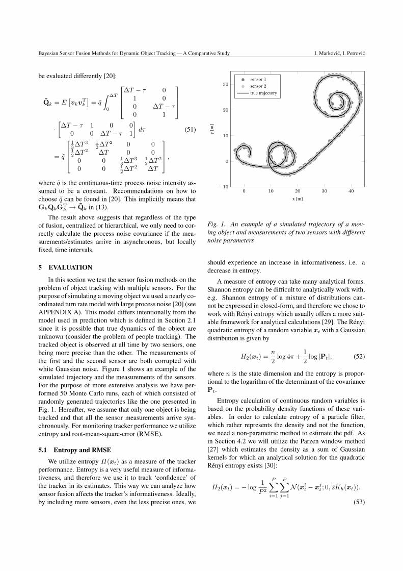
In this section we test the sensor fusion methods on theproblem of object tracking with multiple sensors. For thepurpose of simulating a moving object we used a nearly co-ordinated turn rate model with large process noise [20] (seeAPPENDIX A). This model differs intentionally from themodel used in prediction which is defined in Section 2.1since it is possible that true dynamics of the object areunknown (consider the problem of people tracking). Thetracked object is observed at all time by two sensors, onebeing more precise than the other. The measurements ofthe first and the second sensor are both corrupted withwhite Gaussian noise. Figure 1 shows an example of thesimulated trajectory and the measurements of the sensors.For the purpose of more extensive analysis we have per-formed 50 Monte Carlo runs, each of which consisted ofrandomly generated trajectories like the one presented inFig. 1. Hereafter, we assume that only one object is beingtracked and that all the sensor measurements arrive syn-chronously. For monitoring tracker performance we utilizeentropy and root-mean-square-error (RMSE).

5.1 Entropy and RMSE

We utilize entropy H(xt) as a measure of the trackerperformance. Entropy is a very useful measure of informa-tiveness, and therefore we use it to track ‘confidence’ ofthe tracker in its estimates. This way we can analyze howsensor fusion affects the tracker’s informativeness. Ideally,by including more sensors, even the less precise ones, we

0 10 20 30 40−10

0

10

20

30

x [m]

y[m

]

sensor 1sensor 2true trajectory

Fig. 1. An example of a simulated trajectory of a mov-ing object and measurements of two sensors with differentnoise parameters

should experience an increase in informativeness, i.e. adecrease in entropy.

A measure of entropy can take many analytical forms.Shannon entropy can be difficult to analytically work with,e.g. Shannon entropy of a mixture of distributions can-not be expressed in closed-form, and therefore we chose towork with Rényi entropy which usually offers a more suit-able framework for analytical calculations [29]. The Rényiquadratic entropy of a random variable xt with a Gaussiandistribution is given by

H2(xt) =n

2log 4π +

1

2log |Pt|, (52)

where n is the state dimension and the entropy is propor-tional to the logarithm of the determinant of the covariancePt.

Entropy calculation of continuous random variables isbased on the probability density functions of these vari-ables. In order to calculate entropy of a particle filter,which rather represents the density and not the function,we need a non-parametric method to estimate the pdf. Asin Section 4.2 we will utilize the Parzen window method[27] which estimates the density as a sum of Gaussiankernels for which an analytical solution for the quadraticRényi entropy exists [30]:

H2(xt) = − log1

P 2

P∑i=1

P∑j=1

N (xit − x

jt ; 0, 2Kh(xt)).

(53)


Table 1. Evaluation results of the sensor fusion for 50Monte Carlo runs (number of particles was 250)

RMSE position [m] (velocity [m/s])

EIF UIF PF

Centralized 0.11 (0.17) 0.08 (0.17) 0.08 (0.34)Sensor 1 0.19 (0.24) 0.13 (0.32) 0.18 (0.45)Sensor 2 0.12 (0.18) 0.13 (0.34) 0.08 (0.26)

Hierarchical 0.11 (0.17) 0.13 (0.34) 0.09 (0.31)

Arbitrary local EIF local PF fused EIF

0.06 (0.20) 0.25 (0.47) 0.07 (0.34)

local EIF local PF fused PF

0.06 (0.20) 0.25 (0.47) 0.29 (0.60)

Table 2. Evaluation results of the sensor fusion for thegiven synthetic data example (number of particles was1000)

RMSE position [m] (velocity [m/s])

EIF UIF PF

Centralized 0.69 (1.59) 0.46 (0.85) 0.10 (0.59)Sensor 1 1.10 (2.13) 0.23 (0.70) 0.25 (0.98)Sensor 2 0.77 (1.72) 0.22 (0.68) 0.10 (0.66)

Hierarchical 0.70 (1.61) 0.22 (0.69) 0.13 (0.54)

Arbitrary local EIF local PF fused EIF

0.10 (0.66) 0.11 (0.66) 0.09 (0.59)

local EIF local PF fused PF

0.10 (0.66) 0.11 (0.66) 0.11 (0.60)

The RMSE is calculated both for the position and ve-locity as follows

epos =

√√√√ 1

T

T∑k=1

(xt − xt)2 + (yt − yt)2

evel =

√√√√ 1

T

T∑k=1

(ˆxt − xt)2 + (ˆyt − yt)2,

(54)

where T is the simulation length, (xt, yt) are estimated co-ordinates and (xt, yt) are true coordinates at time index k,while (ˆxt, ˆyt) are the estimated velocities and (xt, yt) aretrue velocities at time index k.

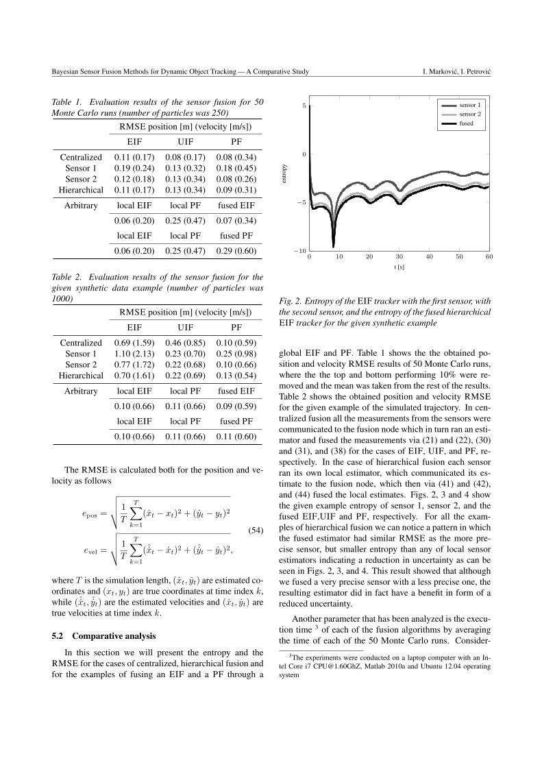
5.2 Comparative analysis

In this section we will present the entropy and theRMSE for the cases of centralized, hierarchical fusion andfor the examples of fusing an EIF and a PF through a

0 10 20 30 40 50 60−10

−5

0

5

t [s]

entr

opy

sensor 1sensor 2fused

Fig. 2. Entropy of the EIF tracker with the first sensor, withthe second sensor, and the entropy of the fused hierarchicalEIF tracker for the given synthetic example

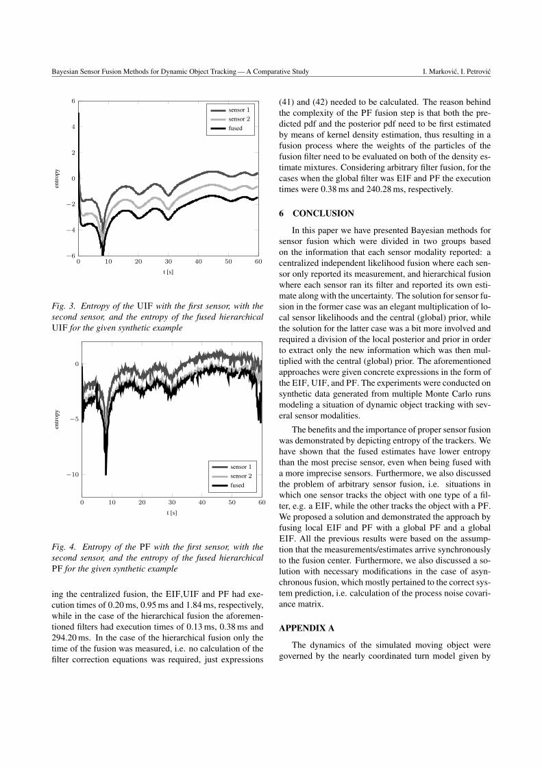
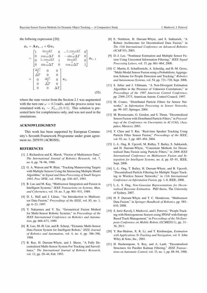
global EIF and PF. Table 1 shows the the obtained po-sition and velocity RMSE results of 50 Monte Carlo runs,where the the top and bottom performing 10% were re-moved and the mean was taken from the rest of the results.Table 2 shows the obtained position and velocity RMSEfor the given example of the simulated trajectory. In cen-tralized fusion all the measurements from the sensors werecommunicated to the fusion node which in turn ran an esti-mator and fused the measurements via (21) and (22), (30)and (31), and (38) for the cases of EIF, UIF, and PF, re-spectively. In the case of hierarchical fusion each sensorran its own local estimator, which communicated its es-timate to the fusion node, which then via (41) and (42),and (44) fused the local estimates. Figs. 2, 3 and 4 showthe given example entropy of sensor 1, sensor 2, and thefused EIF,UIF and PF, respectively. For all the exam-ples of hierarchical fusion we can notice a pattern in whichthe fused estimator had similar RMSE as the more pre-cise sensor, but smaller entropy than any of local sensorestimators indicating a reduction in uncertainty as can beseen in Figs. 2, 3, and 4. This result showed that althoughwe fused a very precise sensor with a less precise one, theresulting estimator did in fact have a benefit in form of areduced uncertainty.

Another parameter that has been analyzed is the execu-tion time 3 of each of the fusion algorithms by averagingthe time of each of the 50 Monte Carlo runs. Consider-

3The experiments were conducted on a laptop computer with an In-tel Core i7 [email protected], Matlab 2010a and Ubuntu 12.04 operatingsystem


0 10 20 30 40 50 60−6

−4

−2

0

2

4

6

t [s]

entr

opy


Fig. 3. Entropy of the UIF with the first sensor, with thesecond sensor, and the entropy of the fused hierarchicalUIF for the given synthetic example

0 10 20 30 40 50 60

−10

−5

0

t [s]

entr

opy


Fig. 4. Entropy of the PF with the first sensor, with thesecond sensor, and the entropy of the fused hierarchicalPF for the given synthetic example

ing the centralized fusion, the EIF,UIF and PF had exe-cution times of 0.20 ms, 0.95 ms and 1.84 ms, respectively,while in the case of the hierarchical fusion the aforemen-tioned filters had execution times of 0.13 ms, 0.38 ms and294.20 ms. In the case of the hierarchical fusion only thetime of the fusion was measured, i.e. no calculation of thefilter correction equations was required, just expressions

(41) and (42) needed to be calculated. The reason behindthe complexity of the PF fusion step is that both the pre-dicted pdf and the posterior pdf need to be first estimatedby means of kernel density estimation, thus resulting in afusion process where the weights of the particles of thefusion filter need to be evaluated on both of the density es-timate mixtures. Considering arbitrary filter fusion, for thecases when the global filter was EIF and PF the executiontimes were 0.38 ms and 240.28 ms, respectively.

6 CONCLUSION

In this paper we have presented Bayesian methods forsensor fusion which were divided in two groups basedon the information that each sensor modality reported: acentralized independent likelihood fusion where each sen-sor only reported its measurement, and hierarchical fusionwhere each sensor ran its filter and reported its own esti-mate along with the uncertainty. The solution for sensor fu-sion in the former case was an elegant multiplication of lo-cal sensor likelihoods and the central (global) prior, whilethe solution for the latter case was a bit more involved andrequired a division of the local posterior and prior in orderto extract only the new information which was then mul-tiplied with the central (global) prior. The aforementionedapproaches were given concrete expressions in the form ofthe EIF, UIF, and PF. The experiments were conducted onsynthetic data generated from multiple Monte Carlo runsmodeling a situation of dynamic object tracking with sev-eral sensor modalities.

The benefits and the importance of proper sensor fusionwas demonstrated by depicting entropy of the trackers. Wehave shown that the fused estimates have lower entropythan the most precise sensor, even when being fused witha more imprecise sensors. Furthermore, we also discussedthe problem of arbitrary sensor fusion, i.e. situations inwhich one sensor tracks the object with one type of a fil-ter, e.g. a EIF, while the other tracks the object with a PF.We proposed a solution and demonstrated the approach byfusing local EIF and PF with a global PF and a globalEIF. All the previous results were based on the assump-tion that the measurements/estimates arrive synchronouslyto the fusion center. Furthermore, we also discussed a so-lution with necessary modifications in the case of asyn-chronous fusion, which mostly pertained to the correct sys-tem prediction, i.e. calculation of the process noise covari-ance matrix.

APPENDIX A

The dynamics of the simulated moving object weregoverned by the nearly coordinated turn model given by


the follwing expression [20]:

xk = Axk−1 + Gvk

=

1 sinω∆T

ω 0 − 1−cosω∆Tω 0

0 cosω∆T 0 − sinω∆T 00 1−cosω∆T

ω 1 sinω∆Tω 0

0 sinω∆T 0 cosω∆T 1

xk−1

+

∆T 2

2 0 0∆T 0 0

0 ∆T 2

2 00 ∆T 00 0 ∆T

vk,(55)

where the state vector from the Section 2.1 was augmentedwith the turn rate ω = 0.5 rad/s, and the process noise wassimulated with vk ∼ N3×1(0, 0.5). This solution is pre-sented here for completeness only, and was not used in thesimulations.

ACKNOWLEDGMENT

This work has been supported by European Commu-nity’s Seventh Framework Programme under grant agree-ment no. 285939 (ACROSS).

REFERENCES

[1] J. Richardson and K. Marsh, “Fusion of Multisensor Data,”The International Journal of Robotics Research, vol. 7,no. 6, pp. 78–96, 1988.

[2] G. A. Watson and W. Blair, “Tracking Maneuvering Targetswith Multiple Sensors Using the Interacting Multiple ModelAlgorithm,” in Signal and Data Processing of Small Targets1993, Proc SPIE, vol. 1954, pp. 438–447, 1993.

[3] R. Luo and M. Kay, “Multisensor Integration and Fusion inIntelligent Systems,” IEEE Transactions on Systems, Man,and Cybernetics, vol. 19, no. 5, pp. 901–931, 1989.

[4] D. L. Hall and J. Llinas, “An Introduction to Multisen-sor Data Fusion,” Proceedings of the IEEE, vol. 85, no. 1,pp. 6–23, 1997.

[5] Y. Nakamura and Y. Xu, “Geometrical Fusion Methodfor Multi-Sensor Robotic Systems,” in Proceedings of theIEEE International Conference on Robotics and Automa-tion, pp. 668–673, 1989.

[6] R. Luo, M.-H. Lin, and R. Scherp, “Dynamic Multi-SensorData Fusion System for Intelligent Robots,” IEEE Journalof Robotics and Automation, vol. 4, no. 4, pp. 386–396,1988.

[7] B. Rao, H. Durrant-Whyte, and J. Sheen, “A Fully De-centralized Multi-Sensor System For Tracking and Surveil-lance,” The International Journal of Robotics Research,vol. 12, pp. 20–44, Feb. 1993.

[8] E. Nettleton, H. Durrant-Whyte, and S. Sukkarieh, “ARobust Architecture for Decentralised Data Fusion,” inThe 11th International Conference on Advanced Robotics(ICAR’03), 2003.

[9] D.-J. Lee, “Nonlinear Estimation and Multiple Sensor Fu-sion Using Unscented Information Filtering,” IEEE SignalProcessing Letters, vol. 15, pp. 861–864, 2008.

[10] C. Martin, E. Schaffernicht, A. Scheidig, and H.-M. Gross,“Multi-Modal Sensor Fusion using a Probabilistic Aggrega-tion Scheme for People Detection and Tracking,” Roboticsand Autonomous Systems, vol. 54, pp. 721–728, Sept. 2006.

[11] S. Julier and J. Uhlmann, “A Non-Divergent EstimationAlgorithm in the Presence of Unknown Correlations,” inProceedings of the 1997 American Control Conference,pp. 2369–2373, American Autom. Control Council, 1997.

[12] M. Coates, “Distributed Particle Filters for Sensor Net-works,” in Information Processing in Sensor Networks,pp. 99–107, Springer, 2004.

[13] M. Rosencrantz, G. Gordon, and S. Thrun, “DecentralizedSensor Fusion with Distributed Particle Filters,” in Proceed-ings of the Conference on Uncertainty in AI (UAI), (Aca-pulco, Mexico), 2003.

[14] Y. Chen and Y. Rui, “Real-time Speaker Tracking UsingParticle Filter Sensor Fusion,” Proceedings of the IEEE,vol. 92, no. 3, pp. 485–494, 2004.

[15] L.-L. Ong, B. Upcroft, M. Ridley, T. Bailey, S. Sukkarieh,and H. Durrant-Whyte, “Consistent Methods for Decen-tralised Data Fusion using Particle Filters,” in 2006 IEEEInternational Conference on Multisensor Fusion and In-tegration for Intelligent Systems, no. d, pp. 85–91, IEEE,Sept. 2006.

[16] L.-L. Ong, T. Bailey, H. Durrant-Whyte, and B. Upcroft,“Decentralised Particle Filtering for Multiple Target Track-ing in Wireless Sensor Networks,” in 11th InternationalConference on Information Fusion, pp. 1–8, IEEE, 2008.

[17] L.-L. S. Ong, Non-Gaussian Representations for Decen-tralised Bayesian Estimation. PhD thesis, The Universityof Sydney, 2007.

[18] H. F. Durrant-Whyte and T. C. Henderson, “MultisensorData Fusion,” in Springer Handbook of Robotics, pp. 585–610, 2008.

[19] S. Juric-Kavelj, I. Markovic, and I. Petrovic, “People Track-ing with Heterogeneous Sensors using JPDAF with EntropyBased Track Management,” in Proceedings of the 5th Euro-pean Conference on Mobile Robots (ECMR2011), pp. 31–36, 2011.

[20] Y. Bar-Shalom, X. R. Li, and T. Kirubarajan, Estimationwith Applications To Tracking and Navigation, vol. 9. JohnWiley & Sons, Inc., 2001.

[21] H. Hashemipour, S. Roy, and A. Laub, “DecentrailzedStructures for Paraller Kalman Filtering,” IEEE Transac-tions on Automatic Control, vol. 33, no. 1, pp. 88–94, 1988.


[22] S. J. Julier and J. K. Uhlmann, “A New Extension of theKalman Filter to Nonlinear Systems,” in International Sym-posium on Aerospace/Defense Sensing, Simulate and Con-trol, vol. 54, (Orlando, FL), 1997.

[23] S. J. Julier, J. K. Uhlmann, and H. F. Durrant-Whyte, “ANew Method for the Nonlinear Transformation of Meansand Covariances in Filters and Estimators,” IEEE Transac-tions on Automatic Control, vol. 45, no. 3, pp. 477–482,2000.

[24] S. Arulampalam, S. Maskell, N. Gordon, and T. Clapp,“A Tutorial on Particle Filters for On-line Non-linear/Non-Gaussian Bayesian Tracking,” Signal Processing, vol. 50,pp. 174–188, 2001.

[25] A. Doucet, N. de Freitas, and N. Gordon, “An Introductionto Sequential Monte Carlo Methods,” in Sequential MonteCarlo Methods in Practice (A. Doucet, N. de Freitas, andN. Gordon, eds.), ch. 1, pp. 3–14, Springer-Verlag, 2001.

[26] D. Fox, “Adapting the Sample Size in Particle Fil-ter Through KLD-Sampling,” International Journal ofRobotics Research, vol. 22, 2003.

[27] E. Parzen, “On Estimation of a Probability Density Func-tion and Mode,” The Annals of Mathematical Statistics,vol. 33, no. 3, pp. 1065–1076, 1962.

[28] C. Musso, N. Oudjane, and F. Le Gland, “Improving Regu-larised Particle Filters,” in Sequential Monte Carlo Methodsin Practice (A. Doucet, N. de Freitas, and N. Gordon, eds.),pp. 247–272, Springer-Verlag, 2001.

[29] T. M. Cover and J. A. Thomas, Elements of InformationTheory. John Wiley & Sons, Inc., 2006.

[30] K. Torkkola, “Feature Extraction by Non-Parametric Mu-tual Information Maximization,” Journal of MachineLearning Research, vol. 3, pp. 1415–1438, Oct. 2003.

Ivan Markovic received the B.Sc. and the Ph.D.degree in Electrical Engineering from the Uni-versity of Zagreb, Faculty of Electrical Engineer-ing and Computing (FER), Croatia in 2008 and2014, respectively. He is currently employed atthe FER, Zagreb, as a Research and Teaching As-sistant funded by the Ministry of Science, Educa-tion and Sport, Republic of Croatia. During hisundergraduate studies, for outstanding academicachievements, he received the “Institute for Nu-clear Technology Award” and the “Josip Loncar

Award” in 2007 and 2006, respectively. In 2013 and 2014 he was a visit-ing researcher at Inria Rennes-Bretagne Atlantique in the Lagadic groupdirected by Prof. François Chaumette, Ph.D. His main research interestsare in mobile robotics, estimation theory and human–robot interaction.

Ivan Petrovic received B.Sc. degree in 1983,M.Sc. degree in 1989 and Ph.D. degree in 1998,all in Electrical Engineering from the Faculty ofElectrical Engineering and Computing (FER Za-greb), University of Zagreb, Croatia. He hadbeen employed as an R&D engineer at the In-stitute of Electrical Engineering of the KoncarCorporation in Zagreb from 1985 to 1994. Since1994 he has been with FER Zagreb, where he iscurrently a full professor and the head of the De-partment of Control and Computer Engineering.

He teaches a number of undergraduate and graduate courses in the fieldof control systems and mobile robotics. His research interests includevarious advanced control strategies and their applications to control ofcomplex systems and mobile robots navigation. Results of his researcheffort have been implemented in several industrial products. He is a mem-ber of IEEE, IFAC – TC on Robotics and FIRA – Executive committee.He is a collaborating member of the Croatian Academy of Engineering.

AUTHORS’ ADDRESSESIvan Markovic, Ph.D.Prof. Ivan Petrovic, Ph.D.University of Zagreb,Faculty of Electrical Engineering and Computing,Department of Control and Computer Engineering,Unska 3, HR-10000, Zagreb, Croatiaemail: {ivan.markovic, ivan.petrovic}@fer.hr

Bayesian Sensor Fusion Methods for Dynamic Object Tracking—A Comparative Study · ·...

Documents

Transcript of Bayesian Sensor Fusion Methods for Dynamic Object Tracking—A Comparative Study · ·...