Bayesian Multi-target Tracking with Merged …ba-ngu.vo-au.com/vo/BVV_MM_TSP15.pdf · Bayesian...

PREPRINT: IEEE TRANSACTIONS ON SIGNAL PROCESSING, VOL. 63, NO. 6, PP. 1433-1447, MARCH 2015 1

Bayesian Multi-target Tracking with MergedMeasurements Using Labelled Random Finite Sets

Michael Beard, Ba-Tuong Vo, and Ba-Ngu Vo

Abstract—Most tracking algorithms in the literature assumethat the targets always generate measurements independently ofeach other, i.e. the sensor is assumed to have infinite resolution.Such algorithms have been dominant because addressing thepresence of merged measurements increases the computationalcomplexity of the tracking problem, and limitations on computingresources often make this infeasible. When merging occurs, thesealgorithms suffer degraded performance, often due to tracksbeing terminated too early. In this paper, we use the theory ofrandom finite sets (RFS) to develop a principled Bayesian solutionto tracking an unknown and variable number of targets in thepresence of merged measurements. We propose two tractableimplementations of the resulting filter, with differing compu-tational requirements. The performance of these algorithms isdemonstrated by Monte Carlo simulations of a multi-targetbearings-only scenario, where measurements become merged dueto the effect of finite sensor resolution.

Index Terms—Multi-target tracking, merged measuremnts,unresolved targets, random finite sets

I. INTRODUCTION

THE sensor models used by the majority of traditionalmulti-target tracking algorithms are based on the assump-

tion that each target generates measurements independently.While this facilitates the development of computationallycheaper tracking algorithms, most real-world sensors violatethis assumption when targets become close together in themeasurement space. A common situation that involves mergedmeasurements is when the sensor has finite resolution [1]. Forexample, most radar and sonar systems divide the measure-ment space into discrete detection cells, and when multipletargets fall within the same cell, they result in a mergedmeasurement. Another example where merging occurs is incomputer vision, where detection algorithms often producemerged measurements for groups of objects appearing closetogether or occluding one-another in an image. In such cases,sensors often generate fewer measurements than there aretargets present, where groups of closely spaced targets producemerged measurements. If the tracking algorithm assumes thateach target generates a measurement independent of eachother, it will usually infer that some targets have disappeared,when in fact their measurements have become merged.

This work was supported in part by the Australian Research Council underFuture Fellowship FT0991854, and Discovery Project DE120102388.

M. Beard is with the Defence Science and Technology Organisa-tion, Rockingham, WA, Australia, and the Department of Electrical andComputer Engineering, Curtin University, Bentley, WA, Australia (email:[email protected]).

B.-T. Vo and B.-N. Vo are with the Department of Electrical and Com-puter Engineering, Curtin University, Bentley, WA, Australia (email: ba-tuong.vo,[email protected]).

Since merged measurements are unavoidable when pro-cessing real world sensor data, and methods that assumeconditionally independent measurements perform poorly whenthis occurs, it is fundamentally important to investigate al-gorithms that can deal with this phenomenon. A numberof Bayesian multi-target tracking algorithms have been pro-posed to handle merged measurements. One such algorithmis Joint Probabilstic Data Association (JPDA), which wasfirst applied to a finite resolution sensor model in [2]. Theproposed algorithm (JPDAM) used a grid-based model forcomputing merging probabilities for two targets, which werethen incorporated into the JPDA update. This technique waslimited to cases where at most two targets are merged at a time.A useful extension to this was proposed in [3], [4] which canhandle an arbirtary number of merged targets, by defining amore general resolution model based on combining pairwisemerging probabilities. This provides a tractable approximationto the probabilities of different resolution events, which areagain incorporated into the JPDA update. The inclusion ofthe resolution model in JPDA has been shown to improveits performance. However, the fundamental limitation of thesemethods is that JPDA implicitly assumes a fixed and knownnumber of targets.

Several other methods have also been applied to mergedmeasurement tracking. An approach based on Multiple Hy-pothesis Tracking (MHT) was proposed in [5], which used atwo-target resolution model to maintain tracks in the pres-ence of merged measurements. A similar resolution modelwas applied to Multiple Model JPDA in [6], [7], which isagain limited to a maximum of two merged targets. Variousnumerical data association techniques have been developed formerged measurements in [8], [9] (Probabilistic Data Associ-ation), and [10] (Markov Chain Monte Carlo). In addition,Probabilistic MHT (PMHT) [11], and existence based methodssuch as Linear Multitarget Integrated PDA (LM-IPDA) [12],and Integrated Track Splitting (ITS) [13] have also been ap-plied to this problem. These are all useful techniques, however,with the exception of LM-IPDA (which trades off performancefor reduced complexity), they only handle a small numberof targets. Moreover, due to the nature of their formulation,it is difficult to establish any results regarding their Bayesoptimality, in the sense of minimising the posterior Bayes risk[14].

In recent times, the concept of random finite sets (RFS)and the tools provided by Finite Set Statistics (FISST) havereceived a great deal of attention, as they provide a principledframework for multi-object estimation for an unknown andtime-varying number of objects [14]. One of the first meth-

2 PREPRINT: IEEE TRANSACTIONS ON SIGNAL PROCESSING, VOL. 63, NO. 6, PP. 1433-1447, MARCH 2015

ods to be derived using this framework was the ProbabilityHypothesis Density (PHD) filter [15], and Mahler proposeda technique in [16] for applying this filter to unresolvedtargets by modelling the multi-target state as an RFS ofpoint clusters. This is a principled approximation which candeal with a variable number of targets. However, it does notprovide labelled track estimates, and the model is limitedto cases where merged measurements arise only when thetargets are close together in the state space, as opposed tothe measurement space. The latter is important in cases wherethe measurement space is a lower dimensional projection ofthe state space (e.g. bearings-only sensors), because pointswhich are well separated in the state space may become closetogether (and therefore unresolvable) when projected onto themeasurement space.

One critisism of the RFS framework has been that it resultedin algorithms that do not maintain target labels over time,i.e. performing multi-object filtering as opposed to tracking. Itwas shown in [17], [18] that the RFS framework does allowestimation of target tracks, and a computationally feasiblemulti-target tracker for the standard sensor model was derived,known as the generalised labelled multi-Bernoulli (GLMB)filter. Our goal in this paper is to further generalise the resultof [17] to a sensor model that includes merged measurements,thereby making it suitable for application to a wider varietyof real world problems. To achieve this, we introduce a multi-target likelihood function that takes into account the possiblemerging of target generated measurements, by consideringfeasible partitions of the target set, and the feasible assign-ments of measurements to groups within these partitions. Toour knowledge, this is the first provably Bayes optimal multi-object tracker that accommodates merged measurements, withtime varying and unknown number of targets. An advantage ofour approach is that it can be parallelised to facilitate potentialreal-time implementation.

Preliminary results of this work have been presented in [20],which this paper builds upon by including a more completeexposition of the derivation and implementation of the mergedmeasurement GLMB filter, including detailed pseudo-code.Furthermore, we propose a computationally cheaper variantof the algorithm using relaxed measurement assignment, anda more extensive simulation study is presented.

The paper is organised as follows. Section II provides somebackground on labelled random finite sets and their applicationto tracking with standard sensor models. In Section III wepropose a merged measurement likelihood model, and uselabelled random finite sets to develop a filter based on thismodel. Section IV presents an approximation technique, andintroduces two methods to aid in its tractable implementation.Further details and pseudo-code are given in Section V.Section VI contains simulation results for a bearings-onlymulti-target tracking scenario, and finally, some concludingremarks are given in Section VII.

II. BACKGROUND: RFS-BASED TRACKING WITHSTANDARD SENSOR MODELS

The goal of recursive multi-object Bayesian estimation is toestimate a finite set of states Xk ⊂ X, called the multi-object

state, at each time k. The multi-object states Xk and multi-object observations Zk ⊂ Z are modelled as random finitesets, and FISST is a framework for working with RFSs [14]based on a notion of integration/density that is consistent withpoint process theory [19].

At the previous time step k − 1, the multi-object state isassumed to be distributed according to a multi-object densityπk−1 (·|Z1:k−1), where Z1:k−1 is an array of finite sets ofmeasurements recieved up to time k− 1. Each Zk is assumedto be generated through a process of thinning of misdetectedobjects, Markov shifts of detected objects, and superpositionof false measurements. The multi-object prediction to time kis given by the Chapman-Kolmogorov equation

πk|k−1 (Xk|Z1:k−1) =

∫fk|k−1 (Xk|X)πk−1 (X|Z1:k−1) δX,

(1)where fk|k−1 (Xk|X) is the multi-object transition kernel fromtime k − 1 to time k, and the integral is the set integral,∫

f (X) δX =

∞∑i=0

1

i!

∫Xif (x1, . . . , xi) d (x1, . . . , xi)

(2)for any function f that takes F (X), the collection of all finitesubsets of X, to the real line. A new set of observationsZk is received at time k, which is modelled by a multi-object likelihood function gk (Zk|Xk). Thus the multi-objectposterior at time k is given by Bayes rule

πk (Xk|Z1:k) =gk (Zk|Xk)πk|k−1 (Xk|Z1:k−1)∫gk (Zk|X)πk|k−1 (X|Z1:k−1) δX

. (3)

Collectively, (1) and (3) are referred to as the multi-objectBayes filter. In general, computing the exact multi-objectposterior is numerically intractable, and approximations arerequired to derive practical algorithms.

One of the first algorithms to be derived based on theseconcepts was the probability hypothesis density (PHD) filter[15], which achieves a tractable approximation to (3) bypropagating only the first moment of the multi-object density.This was followed by the cardinalised PHD (CPHD) filter [22],which propagates the probability distribution on the numberof targets, in addition to the first moment of the multi-objectdensity. Another type of algorithm based on RFSs involvesapproximating the density as a multi-Bernoulli RFS, known asmulti-object multi-Bernoulli (MeMBer) filtering [14], [23]. Acommon feature of the PHD and multi-Bernoulli approaches isthat they do not require data association. However, a significantdrawback is that they do not inherently produce target tracks,instead providing a set of unlabelled target estimates at eachtime step. A recently proposed technique to address thisproblem, which maintains the mathematical rigor of the RFSframework, is the concept of labelled random finite sets [17].This technique involves assigning a distinct label to eachelement of the target set, so that the history of each object’strajectory can be naturally identified.

In this work, we are interested in algorithms that canproduce continuous tracks, so we restrict our attention tomethods based on labelled random finite sets. In [17] and [18],

BEARD et al.: BAYESIAN MULTI-TARGET TRACKING WITH MERGED MEASUREMENTS USING LABELLED RANDOM FINITE SETS 3

an algorithm was proposed for solving the standard multi-object tracking problem, based on a type of labelled RFScalled generalised labelled multi-Bernoulli (GLMB). We nowreview the main points of this technique, and in the nextsection we propose a generalisation, enabling it to handlemerged measurements.

We begin by introducing some notation and definitions relat-ing to labelled random finite sets. The multi-object exponentialof a real valued function h raised to a set X is definedas [h]

X ,∏x∈X h (x), where [h]

∅= 1, and the elements

of X may be of any type such as scalars, vectors, or sets,provided that the function h takes an argument of that type.The generalised Kronecker delta function is defined as

δY (X) ,

1, if Y = X

0, otherwise(4)

where again, X and Y may be of any type, such as scalars,vectors, or sets. Finally, the set inclusion function is

1Y (X) ,

1, if X ⊆ Y0, otherwise

. (5)

In general, we adopt the notational convention that labelledsets are expressed in bold upper case (X), unlabelled sets inregular upper case (X), labelled vectors in bold lower case(x), and unlabelled vectors or scalars in regular lower case(x). The pseudo-code in Section V does not strictly adhere tothis convention, however, any exceptions should be clear fromthe context. We also use the notation x1:n ≡ (x1, . . . , xn) toabbreviate arrays, and x1:n ≡ x1, . . . , xn for sets.

Definition 1. A labelled RFS with state space X and discretelabel space L, is an RFS on X×L, such that the labels withineach realisation are always distinct. That is, if LX is the set ofunique labels in X , and we define the distinct label indicatorfunction as ∆ (X) = δ|X| (|LX |), then a realisation X of alabelled RFS always satisfies ∆ (X) = 1.

Definition 2. A generalised labelled multi-Bernoulli (GLMB)RFS is a labelled RFS with state space X and discrete labelspace L, which satisfies the probability distribution

π (X) = ∆ (X)∑c∈C

w(c) (LX)[p(c) (·)

]X(6)

where C is an arbitrary index set,∑L⊆L

∑c∈C w

(c) (L) = 1,and

∫x∈X p

(c) (x, l) dx = 1.

The GLMB, as defined above, has been shown to be aconjugate prior with respect to the standard multi-objecttransition and multi-object observation functions [17] (i.e.the form of the density is retained through both predictionand update), which facilitates implementation of a BayesianGLMB filter.

A. Multi-object Transition Kernel

Let X be the labelled RFS of objects at the current timewith label space L. A particular object (x, l) ∈ X hasprobability pS (x, l) of surviving to the next time with state(x+, l+) and probability density f (x+|x, l) δl (l+) (where

f (x+|x, l) is the single target transition kernel), and prob-ability, qS (x, l) = 1−pS (x, l) of being terminated. Thus, theset S of surviving objects at the next time is distributed as

fS (S|X) = ∆ (S) ∆ (X) 1LX(LS) [Φ (S; ·)]X (7)

where

Φ (S;x, l) =∑

(x+,l+)∈S

δl (l+) pS (x, l) f (x+|x, l)

+ (1− 1LS(l)) qS (x, l) . (8)

Now let B be the labelled RFS of newborn objects with labelspace B, where L ∩ B = ∅. To ensure that L and B aredisjoint, we adopt a labelling scheme such that each new birthis labelled with a pair (tb, lb), where tb is the current timeand lb is a unique index. Since the time changes from scanto scan, the space of birth labels is always disjoint from thespace of surviving labels. Since the births have distinct labels,and assuming that their states are independent, we model Baccording to a labelled multi-Bernoulli distribution (LMB)

fB (B) = ∆ (B)wB (LB) [pB (·)]B . (9)

where pB (·, l) is the single target birth density, and wB(·) isthe birth weight (see Section IV-D of [17] for more details).We present the prediction based on an LMB birth model,however, this can easily be extended to the case of a GLMBbirth model. The overall multi-object state at the next time stepis the union of survivals and new births, i.e. X+ = S∪B. Thelabel spaces L and B are disjoint, and the states of new bornobjects are independent of surviving objects, hence S and Bare independent. It was shown in [17] that the multi-objecttransition can be expressed as

f (X+|X) = fS (X+ ∩ (X× L) |X) fB (X+ − (X× L)) ,(10)

and that a GLMB density of the form (6) is closed under theChapman-Kolmogorov prediction (1) with the transition kerneldefined by (10).

B. Standard Multi-object Observation Model

Let X be the labelled RFS of objects that exist at theobservation time. A particular object x ∈ X has probabilitypD (x) of generating a detection z with likelihood g (z|x), andprobability qD (x) = 1− pD (x) of being misdetected. Let Dbe the set of target detections. Assuming the elements of Dare conditionally independent, then D is a multi-Bernoulli RFSwith parameter set (pD (x) , g (·|x)) : x ∈X, and we writeits probability density as

πD (D|X) = (pD (x) , g (·|x)) : x ∈X (D) . (11)

Let K be the set of clutter observations, which are independentof the target detections. We model K as a Poisson RFS withintensity κ(·), hence K is distributed according to

πK (K) = e−〈κ,1〉κK . (12)

The overall multi-object observation is the union of targetdetections and clutter observations, i.e. Z = D ∪ K. Since


D and K are independent, the multi-object likelihood is

g (Z|X) =∑D⊆Z

πD (D|X)πK (Z −D) . (13)

As demonstrated in [14], this can be equivalently expressed as

g (Z|X) = e−〈κ,1〉κZ∑

θ∈Θ(LX)

[ψZ (·; θ)]X (14)

where Θ (LX) is the set of all one-to-one mappings oflabels in X to measurement indices in Z, (i.e. θ : LX →0, 1, ..., |Z|, such that [θ (i) = θ (j) > 0] ⇒ [i = j]), andψZ (·; θ) is

ψZ (x, l; θ) =

pD(x,l)g(zθ(l)|x,l)

κ(zθ(l)), θ (l) > 0

qD (x, l) , θ (l) = 0(15)

It was demonstrated in [17] that a GLMB density of theform (6) is closed under the Bayes update (3) with likelihoodfunction defined by (14).

III. RFS-BASED TRACKING WITH MERGEDMEASUREMENTS

A. Multi-object Likelihood Model for Merged Measurements

In [14], Mahler proposed an RFS-based technique forfiltering with unresolved targets, which modelled the multi-target state as a set of point clusters. A point cluster wasdefined as a group of unresolved targets, and was representedas a location in the single-target state space, augmented witha positive integer which holds the number of targets thatare effectively co-located at that point (relative to the sensorresolution). The likelihood function for this model contains asum over partitions of the measurement set, and therefore adirect implementation would be computationally prohibitive. APHD filter based on this model was proposed in [16], however,it has not been implemented in practice.

The point cluster model is intuitively appealing in caseswhere the measurements only become merged when the targetsare close together in the state space. However, this implicitlyassumes that the merging only depends on the target states.There are important cases where this assumption is too restric-tive, examples of which are bearings-only tracking, and visualtracking. In these cases, targets that cannot be resolved alongthe line of sight may be separated by a considerable distancein the state space. The sensor’s position clearly has an impacton whether measurements become merged, but this cannot beaccounted for using the point cluster model. This occurs ingeneral when the measurement space is a lower dimensionalprojection of the state space, such that well separated statescan potentially give rise to closely spaced measurements.

To address these cases, we require a likelihood function thataccommodates measurement merging, not only when targetsare nearby in the state space, but more generally when theyare nearby in the measurement space. To achieve this, we mustconsider partitions of the target set, where each group withina partition produces at most one (merged) measurement.

Definition 3. A partition of a set A is a disjoint collection ofsubsets of A, whose union is equal to A.

Figure 1 contains an example of some of the partitions ofa set of five targets. In the diagram, only six of the total of15 partitions are shown. In general, the number of partitionsof a set of N targets is given by the N -th Bell number,which becomes extremely large with increasing N . However,in the context of multi-target tracking, it is usually possible toeliminate many partitions from consideration, since they arephysically impossible or extremely unlikely to occur.

Figure 1. Some of the partitions of a set of five targets. Each shaded groupof targets can give rise to at most one measurement.

We define our model for the multi-object measurementlikelihood as a sum over partitions of the target set as follows,

g (Z|X) =∑

U(X)∈P(X)

g (Z|U (X)) (16)

where P (X) is the set of all partitions of X , and g (Z|U (X))is the measurement likelihood conditioned on the targetsbeing observed according to partition U (X). This bears somesimilarity to the approach taken in [4], insofar as they bothconsider partitions of the targets in order to form resolutionevents. However, the key difference is that our likelihood isdefined as a function of a set of target states, instead of avector with fixed dimension. This allows us to utilise FISSTprinciples to arrive at an expression for the posterior density.

To obtain an expression for g (Z|U (X)), we generalise thestandard measurement likelihood in (14) to target groups asfollows1

g (Z|U (X)) = e−〈κ,1〉κZ∑

θ∈Θ(U(LX))

[ψZ(·; θ)

]U(X)(17)

where Θ (U (LX)) is defined as the set of all one-to-onemappings of groups of target labels in U (LX) to measurementindices in Z (i.e. θ : U (LX) → 0, 1, ..., |Z|, where[θ (L) = θ (J) > 0] ⇒ [L = J ]), and ψZ (Y ; θ) is a ‘grouplikelihood’ defined by

ψZ (Y ; θ) =

pD(Y )g

(zθ(LY )|Y

)κ(zθ(LY )

) , θ (LY ) > 0

qD(Y ), θ (LY ) = 0

(18)

where pD (Y ) is the detection probability for target group Y ,qD (Y ) = 1−pD (Y ) is the misdetection probability for groupY , and g

(zθ(LY )|Y

)is the likelihood of measurement zθ(LY )

1For notational convenience, we use U (X) to denote a partition of thelabel-state pairs in the labelled set X , and U (LX) to denote the equivalentpartition of the labels only.


given target group Y . For our simulations in Section VI,g (·|Y ) is modelled as a Gaussian centered around the meanof the group, with group size-dependent standard deviation.However, the form of this function in general will depend onthe sensor characteristics, and there are no restrictions placedon its modelling, provided that it can be tractably computed.Note that in (17), the exponent U (X) is a set of target sets,and the base is a real valued function whose argument is atarget set. Substituting (17) into (16) yields the likelihood

g (Z|X) = e−〈κ,1〉κZ∑

U(X)∈P(X)θ∈Θ(U(LX))

[ψZ (·; θ)

]U(X). (19)

B. A General Form for a Merged Measurement Tracker

Definition 4. A labelled RFS mixture density on state spaceX and discrete label space L, is a density of the form

π (X) = ∆ (X)∑c∈C

w(c) (LX) p(c) (X) (20)

where∑L⊆L

∑c∈C

w(c) (L) = 1, p(c) (X) is symmetric in the

elements of X , and p(c) ((·, l1) , ..., (·, ln)) is a joint pdf inXn.

A labelled RFS mixture density differs from the GLMBdensity of definition 2 in that each p(c) (X) is a joint densityof all the targets in X , whereas in definition 2, it is restrictedto a product of single-target densities. Note that any labelledRFS density can be written in the mixture form (20). We usethe mixture form because it is convenient for the update stepof our proposed tracker.

Proposition 5. If the multi-object prior is a labelled RFSmixture density with probability distribution of the form (20),then the predicted multi-object density under the transitionkernel (10) is given by

π+ (X+) = ∆ (X+)∑c∈C

∑L⊆L

w(c)+,L

(LX+

)p

(c)+,L (X+) (21)

where

w(c)+,L (J) = 1L (J ∩ L)wB (J − L)w(c) (L) η

(c)S (L) (22)

p(c)+,L (X+) = [pB (·)]X+−X×L p

(c)S,L (X+ ∩ X× L) (23)

p(c)S,L (S) =

∫p

(c)l1:|L|

(x1:|L|

) |L|∏i=1

Φ (S;xi, li) dx1:|L|

η(c)S (L)

(24)

η(c)S (L) =

∫ ∫p

(c)l1:|L|

(x1:|L|

) |L|∏i=1

Φ (S;xi, li) dx1:|L|δS

(25)

p(c)l1:|L|

(x1:|L|

)≡ p(c)

((x1, l1) , . . .

(x|L|, l|L|

))(26)

Note that for any function f : F (X× L) → R, we haveused the convention fl1:n (x1:n) = f ((x1, l1) , . . . , (xn, ln))to denote it as a function on Xn, given the labels l1:n.

Proposition 6. If the prior is a labelled RFS mixture densitywith probability distribution of the form (20), then the poste-rior multi-object density under the likelihood function (19) isgiven by

π (X|Z) (27)

= ∆ (X)∑c∈C

∑U(X)∈P(X)θ∈Θ(U(LX))

w(c,θ)Z (U (LX)) p(c,θ) (U (X) |Z)

where

w(c,θ)Z (U (L)) =

w(c) (L) η(c,θ)Z (U (L))∑

c∈C

∑J⊆L

∑U(J)∈P(J)θ∈Θ(U(J))

w(c) (J) η(c,θ)Z (U (J))

(28)

p(c,θ) (U (X) |Z) =

[ψZ (·; θ)

]U(X)p(c) (X)

η(c,θ)Z (U (LX))

(29)

η(c,θ)Z (U (L)) =

∫ [ψZ (·; θ)

]U(L)p

(c)l1:|L|

(x1:|L|

)dx1:|L|

(30)

Proofs of Propositions 5 and 6 are given in the appendix.Technically, the family of labelled RFS mixture densities canbe regarded as a conjugate prior with respect to the mergedmeasurement and standard likelihood functions, due to closureunder the Chapman-Kolmogorov prediction and Bayes update.However, this is a very broad class of priors, and is generallynumerically intractable. For this reason, calling the labelledRFS mixture a conjugate prior may be misleading, so werefrain from using this term.

Although it may be possible to directly implement thefilter from Propositions 5 and 6, it would quickly becomeintractable because there is no clear way of truncating thesum over the space of measurement-to-group associationsΘ (U (LX)). The reason is that each component in the overalldensity (20) consists of a single joint density encompassing alltargets, so there may be dependencies between target groups,meaning that standard ranked assignment techniques cannotbe applied. The next section proposes an approximation andtwo alternative methods for implementing a tractable versionof the GLMB filter for the merged measurement likelihood.

IV. TRACTABLE APPROXIMATIONS

The exact form of the filter as specified in Propositions5 and 6, is intractable due to the presence of joint densitiesp(c) (X) in the prior (20). To derive an algorithm that can beimplemented in practice, we approximate the labelled RFSmixture prior by a GLMB of the form (6). Applying themerged measurement likelihood function to a GLMB prioryields a posterior that is no longer a GLMB, but a labelledRFS mixture. However, by marginalising the joint densitiespost-update, we can approximate the posterior as a GLMB, sothat a recursive filter may be implemented. Moreover, usinga recent result on GLMB density approximation [21], it canbe shown that our GLMB approximation preserves the firstmoment and cardinality distribution.


For a prior density in the form of a GLMB as in (6),applying the likelihood function (19) yields a posterior thatis a labelled RFS mixture given by

π (X|Z) (31)

= ∆ (X)∑c∈C


w(c,θ)Z (U (LX))

[p(c,θ) (·|Z)

]U(X)

where

w(c,θ)Z (U (L)) =

w(c) (L)[η

(c,θ)Z (·)

]U(L)

∑c∈C

∑J⊆L

∑U(J)∈P(J)θ∈Θ(U(J))

w(c) (J)[η

(c,θ)Z (·)

]U(J)

(32)

p(c,θ) (Y |Z) =p(c) (Y ) ψZ (Y ; θ)

η(c,θ)Z (LY )

(33)

p(c) (Y ) =[p(c) (·)

]Y(34)

η(c,θ)Z (L) =

⟨p

(c)l1:|L|

(·) ,(ψZ)l1:|L|

(·; θ)⟩

(35)

and ψZ (Y ; θ) is given by (18). The derivation of this is givenin the appendix. In order to bring the posterior density back tothe required GLMB form, we marginalise the joint densitieswithin each component of the labelled RFS mixture as follows

p(c,θ) (Y |Z) ≈[p(c,θ) (·|Z)

]Y,

p(c,θ)(xi, li|Z) =

∫p

(c,θ)l1:|L|

(x1:|L||Z

)d(x1:i−1, xi+1:|L|

).

This allows us to make the following approximation, sincethe set of joint densities representing the groups in partitionU (X) reduces to a set of independent densities representingthe targets in X ,[

p(c,θ) (·|Z)]U(X)

≈[p(c,θ) (·|Z)

]X.

This leads to the following GLMB approximation to the multi-object posterior

π (X|Z) (36)

≈ ∆ (X)∑c∈C


w(c,θ)Z (U (LX))

[p(c,θ) (·|Z)

]X.

It is clear that computing this posterior will still be verycomputationally demanding, since it consists of a triple-nested sum over prior components, partitions of the targetset, and measurement-to-group associations. In the followingsubsections, we propose two methods of truncating this sumto achieve an efficient implementation of the filter.

A. Partitioning with Constrained Measurement Assignment

The most obvious way to compute the terms in (36) isto list all possible partitions of the target set, and thengenerate assignments of measurements to target groups withineach partition. It is clear that this procedure this will be

computationally prohibitive in cases with a large numberof targets, due to the exponentially increasing number ofpartitions. However, it is possible to remove many of theunlikely partitions by exploiting two pieces of information; thecluster structure of the target set, and a model of the sensor’sresolution capabilities. Target clustering can be exploited byconstructing disjoint subsets of the targets that are known tobe well separated, and which have no possibility of sharingmeasurements. An independent filter is executed for eachcluster, and since each of these filters only needs to partitiona smaller set of targets, this can lead to a significant reductionin the total number of partitions to be computed [24], [25].

A method of further reducing the partitions for each clusteris to use a sensor resolution model to remove those that are un-likely to occur. Various resolution models have been proposedin the literature in order to approximate the probability of aresolution event (or equivalently, a partition of the targets) [2],[5], [4]. It would be possible to use such a model to eliminateunlikely partitions, by only retaining those that exceed someminimum probability threshold. In this paper, we use a simplermodel in order to eliminate the unlikely partitions, since ourfilter does not require the use of partition probabilities. Ourmodel requires two parameters; the maximum spread of targetsin an unresolved group in the measurement space (dtmax),and the minimum distance between centroids of unresolvedgroups in the measurement space (dgmin). A partition U (X)is considered infeasible if either of the following is true,

Dmin

(Y ;Y ∈ U (X)

)< dgmin (37)

max (Dmax(Y );Y ∈ U (X)) > dtmax (38)

where Y is the mean of the set Y , Dmin(Y ) is the minimumpairwise distance between points in Y , and Dmax (Y ) is themaximum pairwise distance between points in Y . This modelcan be applied separately to each measurement dimension,and a partition is rejected if condition (37) is satisfied in alldimensions or condition (38) is satisfied in any dimension.Intuitively, this model enforces the constraint that any unre-solved target group cannot be spread over a large distance,and resolved groups cannot appear too close together. Byapplying these constraints, the unlikely partitions are removed,thereby allowing the filter to devote a larger proportion of itscomputational resources to the more likely partitions.

Having generated the feasible partitions, we can now pro-ceed to compute the terms of the posterior GLMB density.In a manner similar to that of the standard GLMB filter[17], a ranked set of alternative measurement assignments isgenerated using Murty’s algorithm [26]. The difference here isthat instead of assigning measurements to individual targets,we now assign the measurements to groups of targets withineach partition. We refer to this version of the algorithm as theGLMB-MP filter, and a more detailed account of the updateroutine is given in Section V-C.

B. Relaxed Measurement Assignment

The previous section described a method of generatinghighly weighted components from the posterior, however,it is very computationally demanding due to the need to


A

B

C1,1C1,2 C1,3 C1,M

C2,1C2,2 C2,3 C2,M

CN,1 CN,2CN,3 CN,M

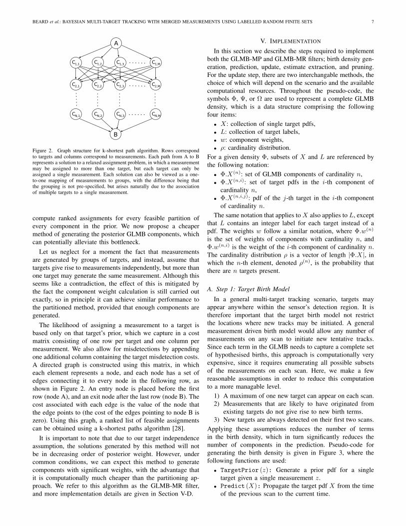
Figure 2. Graph structure for k-shortest path algorithm. Rows correspondto targets and columns correspond to measurements. Each path from A to Brepresents a solution to a relaxed assignment problem, in which a measurementmay be assigned to more than one target, but each target can only beassigned a single measurement. Each solution can also be viewed as a one-to-one mapping of measurements to groups, with the difference being thatthe grouping is not pre-specified, but arises naturally due to the associationof multiple targets to a single measurement.

compute ranked assignments for every feasible partition ofevery component in the prior. We now propose a cheapermethod of generating the posterior GLMB components, whichcan potentially alleviate this bottleneck.

Let us neglect for a moment the fact that measurementsare generated by groups of targets, and instead, assume thattargets give rise to measurements independently, but more thanone target may generate the same measurement. Although thisseems like a contradiction, the effect of this is mitigated bythe fact the component weight calculation is still carried outexactly, so in principle it can achieve similar performance tothe partitioned method, provided that enough components aregenerated.

The likelihood of assigning a measurement to a target isbased only on that target’s prior, which we capture in a costmatrix consisting of one row per target and one column permeasurement. We also allow for misdetections by appendingone additional column containing the target misdetection costs.A directed graph is constructed using this matrix, in whicheach element represents a node, and each node has a set ofedges connecting it to every node in the following row, asshown in Figure 2. An entry node is placed before the firstrow (node A), and an exit node after the last row (node B). Thecost associated with each edge is the value of the node thatthe edge points to (the cost of the edges pointing to node B iszero). Using this graph, a ranked list of feasible assignmentscan be obtained using a k-shortest paths algorithm [28].

It is important to note that due to our target independenceassumption, the solutions generated by this method will notbe in decreasing order of posterior weight. However, undercommon conditions, we can expect this method to generatecomponents with significant weights, with the advantage thatit is computationally much cheaper than the partitioning ap-proach. We refer to this algorithm as the GLMB-MR filter,and more implementation details are given in Section V-D.

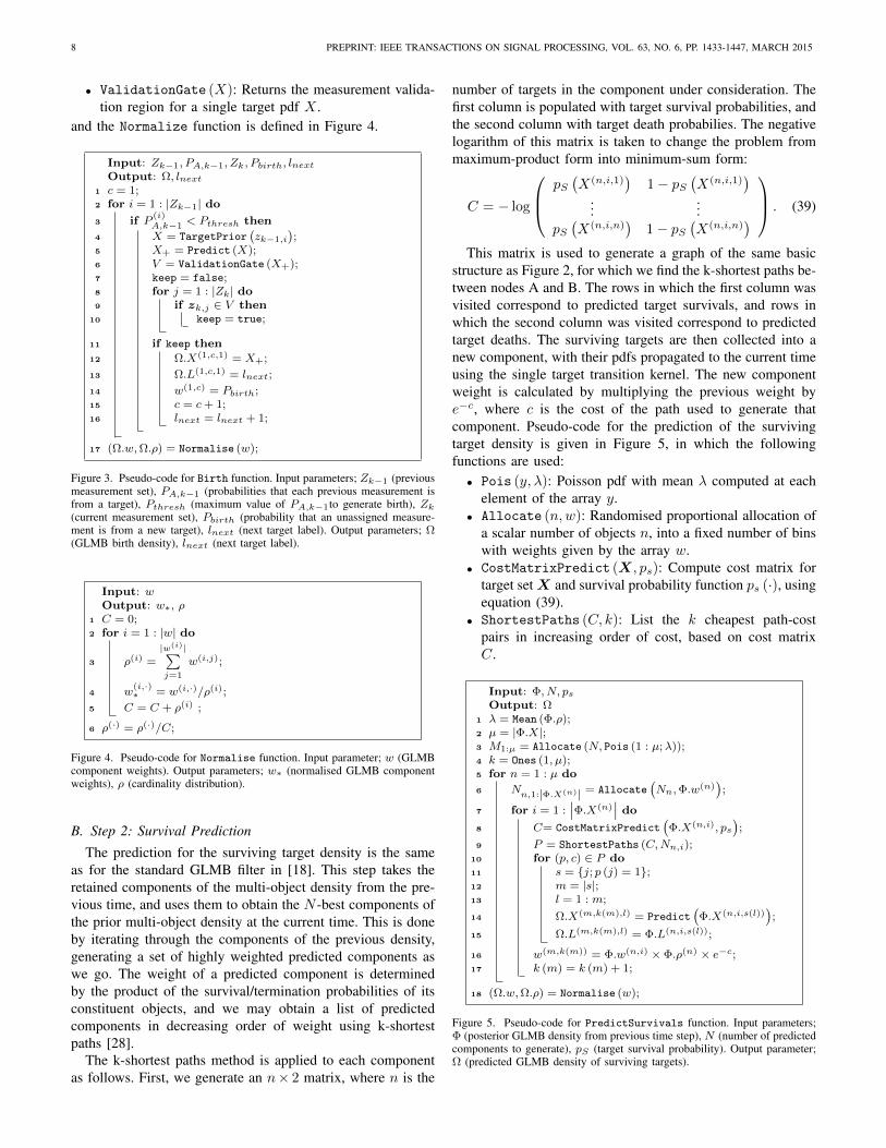
V. IMPLEMENTATION

In this section we describe the steps required to implementboth the GLMB-MP and GLMB-MR filters; birth density gen-eration, prediction, update, estimate extraction, and pruning.For the update step, there are two interchangable methods, thechoice of which will depend on the scenario and the availablecomputational resources. Throughout the pseudo-code, thesymbols Φ, Ψ, or Ω are used to represent a complete GLMBdensity, which is a data structure comprising the followingfour items:• X: collection of single target pdfs,• L: collection of target labels,• w: component weights,• ρ: cardinality distribution.

For a given density Φ, subsets of X and L are referenced bythe following notation:• Φ.X(n): set of GLMB components of cardinality n,• Φ.X(n,i): set of target pdfs in the i-th component of

cardinality n,• Φ.X(n,i,j): pdf of the j-th target in the i-th component

of cardinality n.The same notation that applies to X also applies to L, except

that L contains an integer label for each target instead of apdf. The weights w follow a similar notation, where Φ.w(n)

is the set of weights of components with cardinality n, andΦ.w(n,i) is the weight of the i-th component of cardinality n.The cardinality distribution ρ is a vector of length |Φ.X|, inwhich the n-th element, denoted ρ(n), is the probability thatthere are n targets present.

A. Step 1: Target Birth Model

In a general multi-target tracking scenario, targets mayappear anywhere within the sensor’s detection region. It istherefore important that the target birth model not restrictthe locations where new tracks may be initiated. A generalmeasurement driven birth model would allow any number ofmeasurements on any scan to initiate new tentative tracks.Since each term in the GLMB needs to capture a complete setof hypothesised births, this approach is computationally veryexpensive, since it requires enumerating all possible subsetsof the measurements on each scan. Here, we make a fewreasonable assumptions in order to reduce this computationto a more managable level.

1) A maximum of one new target can appear on each scan.2) Measurements that are likely to have originated from

existing targets do not give rise to new birth terms.3) New targets are always detected on their first two scans.

Applying these assumptions reduces the number of termsin the birth density, which in turn significantly reduces thenumber of components in the prediction. Pseudo-code forgenerating the birth density is given in Figure 3, where thefollowing functions are used:• TargetPrior (z): Generate a prior pdf for a single

target given a single measurement z.• Predict (X): Propagate the target pdf X from the time

of the previous scan to the current time.


• ValidationGate (X): Returns the measurement valida-tion region for a single target pdf X .

and the Normalize function is defined in Figure 4.

Input: Zk−1, PA,k−1, Zk, Pbirth, lnext

Output: Ω, lnext

1 c = 1;2 for i = 1 : |Zk−1| do3 if P

(i)A,k−1 < Pthresh then

4 X = TargetPrior(zk−1,i

);

5 X+ = Predict (X);6 V = ValidationGate (X+);7 keep = false;8 for j = 1 : |Zk| do9 if zk,j ∈ V then

10 keep = true;

11 if keep then

12 Ω.X(1,c,1) = X+;

13 Ω.L(1,c,1) = lnext;

14 w(1,c) = Pbirth;15 c = c+ 1;16 lnext = lnext + 1;

17 (Ω.w,Ω.ρ) = Normalise (w);

Figure 3. Pseudo-code for Birth function. Input parameters; Zk−1 (previousmeasurement set), PA,k−1 (probabilities that each previous measurement isfrom a target), Pthresh (maximum value of PA,k−1to generate birth), Zk

(current measurement set), Pbirth (probability that an unassigned measure-ment is from a new target), lnext (next target label). Output parameters; Ω(GLMB birth density), lnext (next target label).

Input: wOutput: w∗, ρ

1 C = 0;2 for i = 1 : |w| do

3 ρ(i) =|w(i)|∑j=1

w(i,j);

4 w(i,·)∗ = w(i,·)/ρ(i);

5 C = C + ρ(i) ;

6 ρ(·) = ρ(·)/C;

Figure 4. Pseudo-code for Normalise function. Input parameter; w (GLMBcomponent weights). Output parameters; w∗ (normalised GLMB componentweights), ρ (cardinality distribution).

B. Step 2: Survival Prediction

The prediction for the surviving target density is the sameas for the standard GLMB filter in [18]. This step takes theretained components of the multi-object density from the pre-vious time, and uses them to obtain the N -best components ofthe prior multi-object density at the current time. This is doneby iterating through the components of the previous density,generating a set of highly weighted predicted components aswe go. The weight of a predicted component is determinedby the product of the survival/termination probabilities of itsconstituent objects, and we may obtain a list of predictedcomponents in decreasing order of weight using k-shortestpaths [28].

The k-shortest paths method is applied to each componentas follows. First, we generate an n× 2 matrix, where n is the

number of targets in the component under consideration. Thefirst column is populated with target survival probabilities, andthe second column with target death probabilies. The negativelogarithm of this matrix is taken to change the problem frommaximum-product form into minimum-sum form:

C = − log

pS(X(n,i,1)

)1− pS

(X(n,i,1)

)...

...pS(X(n,i,n)

)1− pS

(X(n,i,n)

) . (39)

This matrix is used to generate a graph of the same basicstructure as Figure 2, for which we find the k-shortest paths be-tween nodes A and B. The rows in which the first column wasvisited correspond to predicted target survivals, and rows inwhich the second column was visited correspond to predictedtarget deaths. The surviving targets are then collected into anew component, with their pdfs propagated to the current timeusing the single target transition kernel. The new componentweight is calculated by multiplying the previous weight bye−c, where c is the cost of the path used to generate thatcomponent. Pseudo-code for the prediction of the survivingtarget density is given in Figure 5, in which the followingfunctions are used:• Pois (y, λ): Poisson pdf with mean λ computed at each

element of the array y.• Allocate (n,w): Randomised proportional allocation of

a scalar number of objects n, into a fixed number of binswith weights given by the array w.

• CostMatrixPredict (X, ps): Compute cost matrix fortarget set X and survival probability function ps (·), usingequation (39).

• ShortestPaths (C, k): List the k cheapest path-costpairs in increasing order of cost, based on cost matrixC.

Input: Φ, N, psOutput: Ω

1 λ = Mean (Φ.ρ);2 µ = |Φ.X|;3 M1:µ = Allocate (N, Pois (1 : µ;λ));4 k = Ones (1, µ);5 for n = 1 : µ do

6 Nn,1:|Φ.X(n)| = Allocate(Nn,Φ.w(n)

);

7 for i = 1 :∣∣Φ.X(n)

∣∣ do8 C= CostMatrixPredict

(Φ.X(n,i), ps

);

9 P = ShortestPaths (C,Nn,i);10 for (p, c) ∈ P do11 s = j; p (j) = 1;12 m = |s|;13 l = 1 : m;

14 Ω.X(m,k(m),l) = Predict(Φ.X(n,i,s(l))

);

15 Ω.L(m,k(m),l) = Φ.L(n,i,s(l));

16 w(m,k(m)) = Φ.w(n,i) × Φ.ρ(n) × e−c;17 k (m) = k (m) + 1;

18 (Ω.w,Ω.ρ) = Normalise (w);

Figure 5. Pseudo-code for PredictSurvivals function. Input parameters;Φ (posterior GLMB density from previous time step), N (number of predictedcomponents to generate), pS (target survival probability). Output parameter;Ω (predicted GLMB density of surviving targets).


C. Step 3: Partitioning with Constrained Assignment

The update routine for the GLMB-MP filter involves gener-ating a set of posterior components for each component in theprior, by enumerating the feasible partitions and measurement-to-group assignments. Note that this procedure can be eas-illy parallelised, since there is no dependency between priorcomponents. The first step is to decide how many posteriorcomponents to generate for each prior component. We do thisby allocating a number of components Nn to each cardinalityc, based on a Poisson distribution centered around the meanprior cardinality. This ensures that enough components aregenerated for a variety of cardinalities, to allow for targetbirths and deaths. For each cardinality, we then split up Nnamong the components of cardinality n, where the numberNn,i allocated to component i is proportional to its priorweight. Since it is usually not possible to do this exactlyfor integer numbers of components, we use a randomisedproportional allocation algorithm for this purpose.

For each component, we compute the feasible partitions ofthe target set using the constraints (37) and (38). The numberof allocated components Nn,i is then divided equally amongthese partitions, where the number of components allocated topartition U of the i-th component of cardinality n is denotedNn,i,U . We then compute an assignment cost matrix for eachfeasible partition.

Let X be a set of targets and U (X) a partition of thosetargets. Each row of the cost matrix corresponds to an elementof U (X) (a target group), and each column corresponds to ameasurement, or a misdetection. The cost matrix is of the formC = [D;M ], where D is a |U (X)| × |Z| matrix and M is a|U (X)| × |U (X)| matrix with elements

Di,j = − log

(pD(U (i) (X))g

(zj |U (i) (X)

)κ (zj)

)(40)

Mi,j =

− log

(qD(U (i) (X)

), i = j

∞, i 6= j(41)

where U (i) (X) denotes the i-th group in partition U (X).We now run Murty’s ranked assignment algorithm [26] onthe cost matrix C to obtain a list of the cheapest Nc,k,Umeasurement-to-group assignments in increasing order of cost2. For each assignment, we create a new posterior component,consisting of one updated joint density for each target groupaccording to (33), (35) and (18). Finally, the posterior densityis approximated in the form of a GLMB by computing themarginal distribution for each target, within each posteriorcomponent. Figure 6 shows pseudo-code for the partitionedupdate routine, where the following new functions are used:• Partition (Y ): List partitions of the set Y .• ConstrainPartitions (P, dgmin, d

tmax): Remove infea-

sible partitions in P , according to (37)-(38).• CostMatrixGrp (Z,X,U): Compute cost matrix for

measurement set Z and target set X grouped accordingto partition U , using (40)-(41).

2In our implementation, we have used the auction algorithm [27] to solvethe optimal assignment problem within each iteration of Murty’s algorithm.

• Murty (C, n): Use Murty’s algorithm to list the top nranked assignments based on cost matrix C.

• JointDensity (X): Join the pdfs in the set X to createa joint density.

• MeasUpdate (Y, z): Update the prior density Y usingmeasurement z.

• Marginal (Y, i): Compute the marginal distribution ofthe i-th target from the joint density Y .

• SumWeightSubsets (w, θ): For each set of componentindices in θ, add up the corresponding weights in w.

Input: Φ, Z,N, λ, V, dgmin, dtmax

Output: Ω, PA

1 ρ = Mean (Φ.ρ);2 N1:|Φ.X| = Allocate (N, Pois (0 : |Φ.X| , ρ));

3 χ (i) = ∅,∀i ∈ 1, .., |Z|;4 for n = 1 : |Ω.X| do5 j = 1;


);

7 for i = 1 :∣∣Φ.X(n)

∣∣ do8 P = Partition

(Φ.X(n,i)

);

9 P = ConstrainPartitions(P, dgmin, d

tmax

);

10 Nn,i,1:|P| = Allocate (Nn,i, Ones(1, |P|)/|P|);11 for U ∈ P do

12 C = CostMatrixGrp(Z,Φ.X(n,i),U

);

13 A = Murty(C,Nn,i,U

);

14 for (a, c) ∈ A do15 t = 1;

16 w(n,j) = ρ(n)λ|Z|V −1e−c;17 for G ∈ U do

18 Y = JointDensity(Φ.X(n,i,G)

);

19 YL = Φ.L(n,i,G);20 if a(G) > 0 then21 Y = MeasUpdate

(Y, za(G)

);

22 χ (a(G)) = χ (a(G)) , (n, j);

23 for k = 1 : |G| do24 Ω.X(n,j,t) = Marginal (Y, k);

25 Ω.L(n,j,t) = Y(k)L ;

26 t = t+ 1;

27 j = j + 1;

28 (Ω.w,Ω.ρ) = Normalise (w);29 PA = SumWeightSubsets (Ω.w, χ);

Figure 6. Pseudo-code for PartitionedUpdate. Input parameters; Φ (priorGLMB density), Z (measurement set), N (number of posterior componentsto generate), λ (clutter intensity), V (measurement space volume), dgmin(minimum spacing between group centroids), dtmax (maximum group spread). Output parameters; Ω (posterior GLMB density), PA (probabilities that eachmeasurement is from a target).

D. Alternative Step 3: Relaxed Assignment

As in the partitioned update routine, we generate a setof posterior components for each component in the prior.However, in the GLMB-MR filter, we use a different meansof choosing the components, leading to a cheaper algorithmwhich is scalable to a larger number of targets per cluster. Herewe forego the enumeration of target partitions and Murty-based ranked assignment, in favour of a relaxed assignmentof measurements to targets. This means that a single mea-surement may be assigned to multiple targets simultaneously,


but each target can still only receive one measurement. Thisleads to a simpler and computationally cheaper algorithm, butas one would expect, the performance is not as good as thepartitioning approach.

For each prior component, the cost matrix consists of onerow for each target, and one column for each measurement,with one extra column for misdetections. Thus, the cost matrixis of the form C = [D;M ], where D is a |X| × |Z| matrixand M is a |X| × 1 matrix with elements

Di,j = − log

(pD(X(i))g

(zj |X(i)

)κ (zj)

)(42)

Mi,1 = − log(qD(X(i)

)(43)

The k-shortest paths algorithm is applied to this matrix toselect components for inclusion in the posterior GLMB.The component weights are computed in the same way asin the partitioned update. However, instead of performingjoint updates for each group followed by marginalisation,we approximate the marginal posterior for each target as theindependently updated prior. This avoids the computationalbottleneck of performing a large number of joint multi-targetupdates (one for every possible target grouping). Instead, onlya single independent update needs to be performed for eachunique single target density contained in the prior GLMB.Pseudo-code is provided in Figure 7, where• CostMatrixIndep (Z,X): Compute cost matrix for

measurement set Z and target set X , assuming indepen-dent measurements, i.e. using (42) and (43).

• Unique (y): List the unique elements of the array y.

E. Step 4: Estimate ExtractionLabelled target estimates are extracted from the posterior

GLMB density by finding the maximum a-posteriori estimateof the cardinality, and then finding the highest weightedcomponent with that cardinality. Pseudo-code for this is givenin Figure 8, where τX is the list of estimated tracks, and τLis the list of corresponding labels.

F. Step 5: PruningTo make the algorithm computationally efficient, we need to

prune the posterior density after each update so that insignifi-cant components do not consume computational resources. Acomponent is retained if it is in the top Ncmin components forits cardinality, or if it is in the top Ntot overall and its ratioto the maximum weighted component is less than a thresholdRmax. Pseudo-code is given in Figure 9, where• [c, i] = Sort (w, ρ): Sort components by their absolute

weight, which for the i-th component of cardinality n isgiven by w(n,i)×ρ(n). The sorted components are indexedby their cardinality c, and their position i.

G. Complete AlgorithmThe last function remaining to be defined is that which

multiplies the birth and surviving GLMB densities to arriveat the overall predicted density. Pseudo-code for this functionis given in Figure 10. The top level recursion for the GLMB-Mfilter is given in Figure 11.

Input: Φ, Z,N, λ, VOutput: Ω, PA

1 ρ = Mean (Φ.ρ);2 N1:|Φ.X| = Allocate (N, Pois (0 : |Φ.X| , ρ));

3 χ (i) = ∅, ∀i ∈ 1, .., |Z|;4 for n = 1 : |Φ.X| do5 j = 1;


);

7 for i = 1 :∣∣Φ.X(n)

∣∣ do8 C = CostMatrixIndep

(Z,Φ.X(n,i)

);

9 A = ShortestPaths (C,Nn,i);10 for (a, c) ∈ A do11 t = 1;

12 w(n,j) = ρ(n)λ|Z|V −1;13 for m ∈ Unique (a) do14 G = k : a(k) = m;15 Y = JointDensity

(Φ.X(n,i,G)

);

16 if m > 0 then17 χ (m) = χ (m) , (n, j);18 w(n,j) = w(n,j)PD (Y ) g (zm|Y );

19 else

20 w(n,j) = w(n,j) (1− PD (Y ));

21 for k = 1 : |G| do22 Ω.X(n,j,t) =

MeasUpdate(Φ.X(n,i,G(k)), zm

);

23 Ω.L(n,j,t) = Φ.L(n,i,G(k));24 t = t+ 1;

25 j = j + 1;

26 (Ω.w,Ω.ρ) = Normalise (w);27 PA = SumWeightSubsets (Ω.w, χ);

Figure 7. Pseudo-code for RelaxedUpdate function. Input parameters;Φ (prior GLMB density), Z (measurement set), N (number of posteriorcomponents to generate), λ (clutter intensity), V (measurement space volume).Output parameters; Ω (posterior GLMB density), PA (probabilities that eachmeasurement is from a target).

Input: τX , τL,Ω, TOutput: τX , τL

1 n = argmaxn

(Ω.ρ(n)

);

2 i = argmaxi

(Ω.w(n,i)

);

3 for j = 1 :∣∣Ω.X(n,i)

∣∣ do4 l = Ω.L(n,i,j);5 if l ∈ τL then

6 τX (l) =[τX (l) ;

(T,Ω.X(n,i,j)

)];

7 else8 τL = [τL; l];

9 τX (l) =[(T,Ω.X(n,i,j)

)];

Figure 8. Pseudo-code for ExtractEstimates function. Input parameters;τX (previous track estimates), τL (previous track labels), Ω (GLMB density),T (current time). Output parameters; τX (updated track estimates), τL(updated track labels).

VI. SIMULATION RESULTS

In this section we test the performance of the two proposedversions of the GLMB-M filter on a simulated multi-targettracking scenario. The sensor generates noisy bearings-onlymeasurements with false alarms and misdetections, and thereare multiple crossing targets, each of which follows a whitenoise acceleration dynamic model. The sensor’s motion com-prises legs of constant velocity, interspersed with constant turn


Input: Φ, Ntot, Ncmin, Rmax

Output: Ω1 [C, I] = Sort (w, ρ);

2 wmin = Ω.w(C(1),I(1))/Rmax;3 Mtot = 0;4 Mcdn = Zeros (|Φ.X|);5 for i = 1 : |C| do6 c = C (i) , s = I (i) ,m = Mcdn (c);

7 keep = (Mtot < Ntot)×(Φ.w(c,s) > wmin

)8 + (m < Ncmin);9 if keep then

10 Ω.X(c,m) = Φ.X(c,s);

11 Ω.L(c,m) = Φ.L(c,s);

12 Ω.w(c,m) = Φ.w(c,s);13 Mtot = Mtot + 1;14 Mcdn (c) = m+ 1;

15 (Ω.w,Ω.ρ) = Normalise (Ω.w);

Figure 9. Pseudo-code for Prune function. Input parameters; Φ (GLMBdensity), Ntot (number of components to retain), Ncmin (minimum numberto retain for any cardinality), Rmax (maximum ratio of highest to lowestcomponent weight). Output parameter; Ω (pruned GLMB density).

Input: Φ,ΨOutput: Ω

1 c = Ones (1, |Φ.X|+ |Ψ.X|);2 for m = 1 : |Φ.X| do3 for n = 1 : |Ψ.X| do4 k = m+ n;

5 for i = 1 :∣∣Φ.X(m)

∣∣ do6 for j = 1 :

∣∣Ψ.X(n)∣∣ do

7 Ω.X(k,c(k)) =[Φ.X(m,i); Ψ.X(n,j)

];

8 Ω.L(k,c(k)) =[Φ.L(m,i); Ψ.L(n,j)

];

9 Ω.w(k,c(k)) = Φ.w(m,i) ×Ψ.w(n,j);10 c (k) = c (k) + 1;

11 (Ω.w,Ω.ρ) = Normalise (Ω.w);

Figure 10. Pseudo-code for Multiply function. Input parameters; Φ (GLMBdensity), Ψ (GLMB density). Output parameter; Ω (multiplied GLMB den-sity).

rate manoeuvres. These manoeuvres improve the observabilityover the course of the simulation.

The target state space is defined in terms of 2D Cartesianposition and velocity vectors, i.e. for target t at time k, x(t)

k =[p

(t)x,k p

(t)y,k p

(t)x,k p

(t)y,k

]T. All targets follow the dynamic

model

xk+1 = Fxk + Γvk (44)

F =

[1 T0 1

]⊗ I2, Γ =

[T 2/2T

]⊗ I2 (45)

where T = 20s is the sensor sampling period, and vk ∼N (0, Q) is a 2 × 1 independent and identically distributedGaussian process noise vector with Q = σ2

vI2 where the stan-dard deviation of the target acceleration is σv = 0.005m/s2.

We have simulated the measurements using two alternativemethods; one based on a detection-level measurement model,and the other based on an image simulation followed bypeak detection. The details of these models are given in thesubsections to follow, and in both cases, the measurement

Input: Z1:N , Npred, Nup, Nret, Ncmin, Rmax

Output: τX , τL1 lnext = 1, τX = ∅, τL = ∅;2 PA,1 = Zeros (1, |Z1|);3 for k = 2 : N do4 Ωb, lnext = Birth

(Zk−1, PA,k−1, Zk, lnext

);

5 if k = 2 then6 Ω+ = Ωb;7 else8 Ωs = PredictSurvivals

(Ωk−1, Npred

);

9 Ω+ = Multiply (Ωs,Ωb);

10 if partitioned then11 Ωk, PA,k = PartitionedUpdate (Ω+, Zk, Nup);12 else13 Ωk, PA,k = RelaxedUpdate (Ω+, Zk, Nup);

14 (τX , τL) = ExtractEstimates (τX , τL,Ωk, Tk);15 Ωk = Prune (Ωk, Nret, Ncmin, Rmax);

Figure 11. GLMB-M filter top level recursion. Input parameters; Z1:N

(measurements), Npred (maximum predicted components), Nup (maximumupdated components), Nret (maximum retained components), Ncmin (mini-mum retained for any cardinality),Rmax (maximum component weight ratio).Output parameters; τX (track estimates), τL (track labels).

function is given by

h(x

(t)k , x

(s)k

)= arctan

(p

(t)y,k − p

(s)x,k

p(t)y,k − p

(s)x,k

). (46)

where x(t)k is the target state vector, and x(s)

k is the sensor statevector. For this analysis, we model the pdf of each target usinga single Gaussian, and the measurement updates are carried outusing the extended Kalman filter (EKF). It is clearly possible touse more sophisticated non-linear filters, such as the unscentedor cubature Kalman filter, or to model the single target pdfsusing more accurate representations such as Gaussian mixturesor particle distributions. These techniques may lead to someperformance improvement, but this analysis is beyond thescope of this paper.

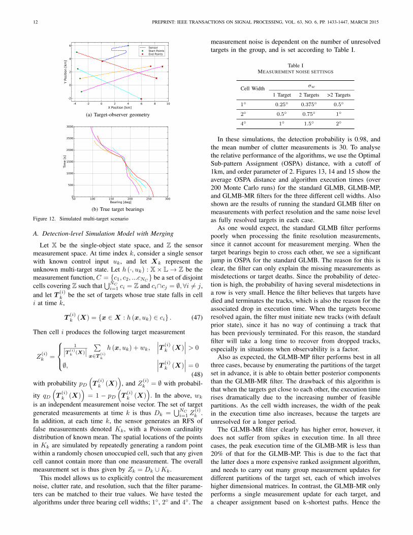
The scenario consists of four targets, with geometry asshown in Figure 12a. One target is present at the beginning,with another three arriving during the first 400 seconds, andthree terminating during the final 900 seconds. The bearings ofall four targets cross one another in the middle of the scenario,which can be seen in Figure 12b. During this time there willbe merged measurements present.

In all cases, the filter initialises the pdf of each newborntarget as a Gaussian with mean range of 10km from thesensor, range standard deviation of 3km, velocity of 5m/smoving directly towards the sensor along the line of bearing,course standard deviation of 50, and speed standard deviationof 2m/s. The filters generate a maximum of Nup = 10000components in the GLMB density during the update, which isreduced to Nret = 1000 (with Ncmin = 10, and Rmax = 108

) during the pruning step. All filters were implemented inC++, and executed on an Intel Core i7 2600 processor. Wehave not parallelised the generation of components in ourimplementation, hence it would be possible significantly speedup the execution time by doing so.


Y Po

sitio

n [k

m]

-2

0

2

4

6

X Position [km]-4 -2 0 2 4 6 8 10

SensorStart PointsEnd Points

(a) Target-observer geometry

Tim

e [s

]

0

500

1000

1500

2000

2500

3000

Bearing [deg]50 100 150 200 250 300

(b) True target bearings

Figure 12. Simulated multi-target scenario

A. Detection-level Simulation Model with Merging

Let X be the single-object state space, and Z the sensormeasurement space. At time index k, consider a single sensorwith known control input uk, and let Xk represent theunknown multi-target state. Let h (·, uk) : X× L→ Z be themeasurement function, C = c1, c2, ...cNC be a set of disjointcells covering Z such that

⋃NCi=1 ci = Z and ci∩cj = ∅,∀i 6= j,

and let T (i)k be the set of targets whose true state falls in cell

i at time k,

T(i)k (X) = x ∈X : h (x, uk) ∈ ci . (47)

Then cell i produces the following target measurement

Z(i)k =

1∣∣∣T (i)

k (X)∣∣∣∑

x∈T (i)k

h (x, uk) + wk,∣∣∣T (i)

k (X)∣∣∣ > 0

∅,∣∣∣T (i)

k (X)∣∣∣ = 0

(48)with probability pD

(T

(i)k (X)

), and Z(i)

k = ∅ with probabil-

ity qD

(T

(i)k (X)

)= 1 − pD

(T

(i)k (X)

). In the above, wk

is an independent measurement noise vector. The set of targetgenerated measurements at time k is thus Dk =

⋃NCi=1 Z

(i)k .

In addition, at each time k, the sensor generates an RFS offalse measurements denoted Kk, with a Poisson cardinalitydistribution of known mean. The spatial locations of the pointsin Kk are simulated by repeatedly generating a random pointwithin a randomly chosen unoccupied cell, such that any givencell cannot contain more than one measurement. The overallmeasurement set is thus given by Zk = Dk ∪Kk.

This model allows us to explicitly control the measurementnoise, clutter rate, and resolution, such that the filter parame-ters can be matched to their true values. We have tested thealgorithms under three bearing cell widths; 1, 2 and 4. The

measurement noise is dependent on the number of unresolvedtargets in the group, and is set according to Table I.

Table IMEASUREMENT NOISE SETTINGS

Cell Width σw

1 Target 2 Targets >2 Targets

1 0.25 0.375 0.5

2 0.5 0.75 1

4 1 1.5 2

In these simulations, the detection probability is 0.98, andthe mean number of clutter measurements is 30. To analysethe relative performance of the algorithms, we use the OptimalSub-pattern Assignment (OSPA) distance, with a cutoff of1km, and order parameter of 2. Figures 13, 14 and 15 show theaverage OSPA distance and algorithm execution times (over200 Monte Carlo runs) for the standard GLMB, GLMB-MP,and GLMB-MR filters for the three different cell widths. Alsoshown are the results of running the standard GLMB filter onmeasurements with perfect resolution and the same noise levelas fully resolved targets in each case.

As one would expect, the standard GLMB filter performspoorly when processing the finite resolution measurements,since it cannot account for measurement merging. When thetarget bearings begin to cross each other, we see a significantjump in OSPA for the standard GLMB. The reason for this isclear, the filter can only explain the missing measurements asmisdetections or target deaths. Since the probability of detec-tion is high, the probability of having several misdetections ina row is very small. Hence the filter believes that targets havedied and terminates the tracks, which is also the reason for theassociated drop in execution time. When the targets becomeresolved again, the filter must initiate new tracks (with defaultprior state), since it has no way of continuing a track thathas been previously terminated. For this reason, the standardfilter will take a long time to recover from dropped tracks,especially in situations when observability is a factor.

Also as expected, the GLMB-MP filter performs best in allthree cases, because by enumerating the partitions of the targetset in advance, it is able to obtain better posterior componentsthan the GLMB-MR filter. The drawback of this algorithm isthat when the targets get close to each other, the execution timerises dramatically due to the increasing number of feasiblepartitions. As the cell width increases, the width of the peakin the execution time also increases, because the targets areunresolved for a longer period.

The GLMB-MR filter clearly has higher error, however, itdoes not suffer from spikes in execution time. In all threecases, the peak execution time of the GLMB-MR is less than20% of that for the GLMB-MP. This is due to the fact thatthe latter does a more expensive ranked assignment algorithm,and needs to carry out many group measurement updates fordifferent partitions of the target set, each of which involveshigher dimensional matrices. In contrast, the GLMB-MR onlyperforms a single measurement update for each target, anda cheaper assignment based on k-shortest paths. Hence the


OSPA

Dis

tanc

e [k

m]

0.0

0.2

0.4

0.6

0.8

1.0

Time [s]0 500 1000 1500 2000 2500 3000

GLMB (1๐)GLMB-MP (1๐)GLMB-MR (1๐)GLMB (perfect)

Exec

utio

n Ti

me

[s]

0.0

0.5

1.0

1.5

2.0

2.5

Time [s]0 500 1000 1500 2000 2500 3000


Figure 13. OSPA distance and execution time: 1 degree resolution

GLMB-MR has a relatively consistent run time, similar to thatof the standard GLMB filter.

OSPA

Dis

tanc

e [k

m]

0.0

0.2

0.4

0.6

0.8

1.0

Time [s]0 500 1000 1500 2000 2500 3000


Exec

utio

n Ti

me

[s]

0.0

0.5

1.0

1.5

2.0

2.5

Time [s]0 500 1000 1500 2000 2500 3000



B. Image-based Simulation Model

The simulation model in the previous section allowed usto explicitly control the clutter rate and measurement noiseparameters via simulation at the detection level. In this sectionwe apply the merged measurement filters to data generatedthrough a more realistic simulation model, in which wegenerate a sensor image, and use a simple peak detector toextract the point measurements. The image is simulated byfirst generating Rayleigh distributed background noise in eachcell. A point spread function is applied to each target toobtain the mean signal amplitude in each cell, and a Riceandistributed signal amplitude is then generated for every cell.This is repeated for all targets, and the signal amplitudes added

OSPA

Dis

tanc

e [k

m]

0.0

0.2

0.4

0.6

0.8

1.0

Time [s]0 500 1000 1500 2000 2500 3000


Exec

utio

n Ti

me

[s]

0.0

0.5

1.0

1.5

2.0

2.5

Time [s]0 500 1000 1500 2000 2500 3000



together in each cell. To generate detections, the vector ofcell amplitudes is interpolated using a spline function, and thelocations of all peaks that exceed a threshold are extracted.Under this model, the combined effect of the cell width andthe point spread function control the distance at which targetsbecome unresolvable. Figure 16 shows an example of theimage generated from this model, with cell width of 1,average signal to noise ratio of 5dB, and a Gaussian pointspread function with standard deviation of 0.5.

Figure 16. Simulated time-bearing image with 1 cell width

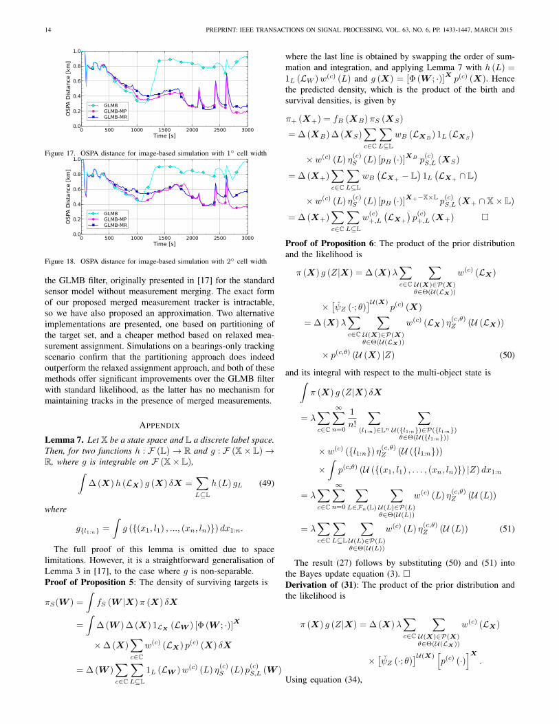
Figures 17 and 18 show the average OSPA distance over200 runs for the standard GLMB, GLMB-MP and GLMB-MR filters, for the case of 1 and 2 cell widths. These resultsfollow the same trend that was observed under the detection-level simulation model. The standard GLMB filter fails due todropped tracks, and the GLMB-MP generally outperforms theGLMB-MR, albeit with a higher computational cost.

VII. CONCLUSION

We have proposed an algorithm for multi-object tracking inthe presence of merged measurements, using the framework oflabelled random finite sets. The algorithm is a generalisation of


OSPA

Dis

tanc

e [k

m]

0.0

0.2

0.4

0.6

0.8

1.0

Time [s]0 500 1000 1500 2000 2500 3000

GLMBGLMB-MPGLMB-MR

Figure 17. OSPA distance for image-based simulation with 1 cell width

OSPA

Dis

tanc

e [k

m]

0.0

0.2

0.4

0.6

0.8

1.0

Time [s]0 500 1000 1500 2000 2500 3000

GLMBGLMB-MPGLMB-MR

Figure 18. OSPA distance for image-based simulation with 2 cell width

the GLMB filter, originally presented in [17] for the standardsensor model without measurement merging. The exact formof our proposed merged measurement tracker is intractable,so we have also proposed an approximation. Two alternativeimplementations are presented, one based on partitioning ofthe target set, and a cheaper method based on relaxed mea-surement assignment. Simulations on a bearings-only trackingscenario confirm that the partitioning approach does indeedoutperform the relaxed assignment approach, and both of thesemethods offer significant improvements over the GLMB filterwith standard likelihood, as the latter has no mechanism formaintaining tracks in the presence of merged measurements.

APPENDIX

Lemma 7. Let X be a state space and L a discrete label space.Then, for two functions h : F (L)→ R and g : F (X× L)→R, where g is integrable on F (X× L),∫

∆ (X)h (LX) g (X) δX =∑L⊆L

h (L) gL (49)

where

gl1:n =

∫g ((x1, l1) , ..., (xn, ln)) dx1:n.

The full proof of this lemma is omitted due to spacelimitations. However, it is a straightforward generalisation ofLemma 3 in [17], to the case where g is non-separable.Proof of Proposition 5: The density of surviving targets is

πS(W ) =

∫fS (W |X)π (X) δX

=

∫∆ (W ) ∆ (X) 1LX

(LW ) [Φ (W ; ·)]X

×∆ (X)∑c∈C

w(c) (LX) p(c) (X) δX

= ∆ (W )∑c∈C

∑L⊆L

1L (LW )w(c) (L) η(c)S (L) p

(c)S,L (W )

where the last line is obtained by swapping the order of sum-mation and integration, and applying Lemma 7 with h (L) =1L (LW )w(c) (L) and g (X) = [Φ (W ; ·)]X p(c) (X). Hencethe predicted density, which is the product of the birth andsurvival densities, is given by

π+ (X+) = fB (XB)πS (XS)

= ∆ (XB) ∆ (XS)∑c∈C

∑L⊆L

wB (LXB) 1L (LXS

)

× w(c) (L) η(c)S (L) [pB (·)]XB p

(c)S,L (XS)

= ∆ (X+)∑c∈C

∑L⊆L

wB(LX+ − L

)1L(LX+ ∩ L

)× w(c) (L) η

(c)S (L) [pB (·)]X+−X×L p

(c)S,L (X+ ∩ X× L)

= ∆ (X+)∑c∈C

∑L⊆L

w(c)+,L

(LX+

)p

(c)+,L (X+)

Proof of Proposition 6: The product of the prior distributionand the likelihood is

π (X) g (Z|X) = ∆ (X)λ∑c∈C


w(c) (LX)

×[ψZ (·; θ)

]U(X)p(c) (X)

= ∆ (X)λ∑c∈C


w(c) (LX) η(c,θ)Z (U (LX))

× p(c,θ) (U (X) |Z) (50)

and its integral with respect to the multi-object state is∫π (X) g (Z|X) δX

= λ∑c∈C

∞∑n=0

1

n!

∑(l1:n)∈Ln

∑U(l1:n)∈P(l1:n)θ∈Θ(U(l1:n))

× w(c) (l1:n) η(c,θ)Z (U (l1:n))

×∫p(c,θ) (U ((x1, l1) , . . . , (xn, ln)) |Z) dx1:n

= λ∑c∈C

∞∑n=0

∑L∈Fn(L)

∑U(L)∈P(L)θ∈Θ(U(L))

w(c) (L) η(c,θ)Z (U (L))

= λ∑c∈C

∑L⊆L

∑U(L)∈P(L)θ∈Θ(U(L))

w(c) (L) η(c,θ)Z (U (L)) (51)

The result (27) follows by substituting (50) and (51) intothe Bayes update equation (3). Derivation of (31): The product of the prior distribution andthe likelihood is

π (X) g (Z|X) = ∆ (X)λ∑c∈C


w(c) (LX)

×[ψZ (·; θ)

]U(X)[p(c) (·)

]X.

Using equation (34),


[p(c) (·)

]U(X)

=∏

Y ∈U(X)

p(c) (Y ) =∏

Y ∈U(X)

[p(c) (·)

]Y=[p(c) (·)

]Xhence we can write

π (X) g (Z|X) = ∆ (X)λ∑c∈C


w(c) (LX)

×[p(c) (·) ψZ (·; θ)

]U(X)

= ∆ (X)λ∑c∈C


w(c) (LX)[η

(c,θ)Z (·)

]U(LX)

×[p(c,θ) (·|Z)

]U(X)

(52)

and its integral∫π (X) g (Z|X) δX

= λ∑c∈C


∫∆ (X)w(c) (LX)

[η

(c,θ)Z (·)

]U(LX)

×[p(c,θ) (·|Z)

]U(X)

δX

= λ∑c∈C


∑L⊆L

w(c) (L)[η

(c,θ)Z (·)

]U(L)

. (53)

The posterior (31)-(35) follows by substitution of (52) and(53) into the Bayes update equation (3).

REFERENCES

[1] F. E. Daum and R. J. Fitzgerald, “The importance of resolution inmultiple target tracking,” Proc. of SPIE 2235, Proc. SPIE Signal &Data Processing of Small Targets , vol. 329, 1994.

[2] K.-C. Chang, Y. Bar-Shalom, “Joint probabilistic data association formultitarget tracking with possibly unresolved measurements and ma-neuvers”, IEEE Trans. Autom. Control, vol. 29, no. 7, pp. 585-594, July1984.

[3] D. Svensson, M. Ulmke, and L. Danielsson, “Joint probabilistic dataassociation filter for partially unresolved target groups”, Proc. 13th Int.Conf. Inform. Fusion, Edinburgh, UK, July 2010.

[4] D. Svensson, M. Ulmke and L. Hammarstrand, “Multitarget SensorResolution Model and Joint Probabilistic Data Association”, IEEETrans. Aerosp. Elecron. Syst., vol. 48, no. 4, pp. 3418-3434, Oct. 2012.

[5] W. Koch, G. van Keuk, “Multiple hypothesis track maintenance withpossibly unresolved measurements”, IEEE Trans. Aerosp. Elecron. Syst.Vol. 33, No. 3, pp. 883-892, July 1997.

[6] H. A. P. Blom, E. A. Bloem, “Bayesian tracking of two possiblyunresolved maneuvering targets”, IEEE Trans. Aerosp. Elecron. Syst.,vol. 43, no. 2, pp. 612-627, Apr. 2007.

[7] S. Jeong, J. K. Tugnait, “Tracking of two targets in clutter with possiblyunresolved measurements”, IEEE Trans. Aerosp. Elecron. Syst., vol. 44,no. 2, pp. 748-765, April 2008.

[8] T. Kirubarajan, Y. Bar-Shalom, K. R. Pattipati, “Multiassignment fortracking a large number of overlapping objects”, IEEE Trans. Aerosp.Electron. Syst., vol. 37, no. 1, pp. 2-21, Jan. 2001.

[9] H. Chen, K. Pattipati, T. Kirubarajan, and Y. Bar-Shalom, "Generaldata association with possibly unresolved measurements using linearprogramming," Proc. Conf. Comput. Vis. Pattern Recog. Workshop(CVPRW), Madison, WI, USA, June 2003.

[10] Z. Khan, T. Balch, and F. Dellaert, “Multitarget tracking with split andmerged measurements”, Proc. IEEE Conf. Computer Vision and PatternRecognition, vol. 1, pp. 605-610, June 2005.

[11] S. J. Davey, “Tracking possibly unresolved targets with PMHT”, Infor-mation, Decision and Control (IDC) 2007, Feb. 2007.

[12] D. Musicki, M. Morelande, “Finite Resolution Multitarget Tracking”,Proc. SPIE Signal and Data Processing of Small Targets, vol. 5913,2005.

[13] D. Musicki, W. Koch, “Multi scan target tracking with finite resolutionsensors”, Proc. 11th Int. Conf. Inform. Fusion, Cologne, Germany, July2008.

[14] R. P. S. Mahler, Statistical Multisource-Multitarget Information Fusion,Artech House, 2007.

[15] R. Mahler, “Multitarget Bayes filtering via first-order multitarget mo-ments”, IEEE Trans. Aerosp. Elecron. Syst., vol. 39, no. 4, pp. 1152-1178, Oct. 2003.

[16] R. Mahler, “PHD filters for nonstandard targets, II: Unresolved targets”,Proc. 12th Int. Conf. Inform. Fusion, pp. 922-929, Seattle, Washington,USA, July 2009.

[17] B.-T. Vo, B.-N. Vo, “Labeled random finite sets and multi-objectconjugate priors”, IEEE Trans. Signal Process., vol. 61, no. 13, pp. 3460-3475, July 2013.

[18] B.-N. Vo, B.-T. Vo, and D. Phung, “Labeled Random Finite Sets andthe Bayes Multi-Target Tracking Filter”, IEEE Trans. Signal Process.,vol. 62, no. 29, pp. 6554-6567, 2014.

[19] B.-N. Vo, S. Singh, and A. Doucet, “Sequential Monte Carlo methods forBayesian Multi-target filtering with Random Finite Sets”, IEEE Trans.Aerosp. Electron. Syst., vol. 41, no. 4, pp. 1224-1245, 2005.

[20] M. Beard, B.-T. Vo, B.-N. Vo, “Multi-target Tracking with MergedMeasurements Using Labelled Random Finite Sets”, Proc. 17th Int.Conf. Inform. Fusion, Salamanca, Spain, July 2014.

[21] F. Papi, B.-N. Vo, B.-T. Vo, C. Fantacci, M. Beard. “GeneralizedLabeled Multi-Bernoulli Approximation of Multi-Object Densities”,arXiv preprint arXiv:1412.5294, December 2014.

[22] R. Mahler, “PHD filters of higher order in target number”, IEEE Trans.Aerosp. and Elec. Syst., vol. 43, no. 4, pp.1523-1543, Oct 2007.

[23] B.-T. Vo, B.-N. Vo, A. Cantoni. “The cardinality balanced multi-targetmulti-Bernoulli filter and its implementations”, IEEE Trans. SignalProcess., vol. 57, no. 2, pp. 409-423, Feb. 2009.

[24] D. B. Reid, “An Algorithm for Tracking Multiple Targets”, IEEE Trans.Autom. Control, vol. AC-24, pp. 843-854, Dec. 1979.

[25] T. Kurien, “Issues in the Design of Practical Multitarget TrackingAlgorithms”, Multisensor-Multitarget Tracking: Advanced ApplicationsVol. 1, pp. 43-83, Artech House, 1990.

[26] K. G. Murty, “An algorithm for ranking all the assignments in increasingorder of cost”, Operations Research, vol. 16, no. 3, pp. 682-678, 1968.

[27] D. P. Bertsekas, “The auction algorithm: A distributed relaxation methodfor the assignment problem”, Annals of Operations Research, vol. 14,no. 1, pp. 105-123, 1988.

[28] J. Y. Yen, “Finding the K-shortest loopless paths in a network”,Management Science, vol. 17, pp. 712-716, 1971.

[29] D. Schuhmacher, B.-T. Vo, B.-N. Vo, “A consistent metric for perfor-mance evaluation of multi-object filters”, IEEE Trans. Signal Process.,vol. 56, no. 8, pp. 3447-3457, Aug. 2008.

Bayesian Multi-target Tracking with Merged …ba-ngu.vo-au.com/vo/BVV_MM_TSP15.pdf · Bayesian...

Documents

Transcript of Bayesian Multi-target Tracking with Merged …ba-ngu.vo-au.com/vo/BVV_MM_TSP15.pdf · Bayesian...