
Bayesian methods for time series with mixed and mixture ...
199
Bayesian methods for time series with mixed and mixture distributions with an application to daily rainfall data Muhammad Safwan Bin Ibrahim Thesis submitted for the degree of Doctor of Philosophy School of Mathematics, Statistics & Physics Newcastle University Newcastle upon Tyne United Kingdom November 2018
Transcript of Bayesian methods for time series with mixed and mixture ...

Bayesian methods for time series with mixedand mixture distributions with an application
to daily rainfall data
Muhammad Safwan Bin Ibrahim
Thesis submitted for the degree ofDoctor of Philosophy
School of Mathematics, Statistics & PhysicsNewcastle UniversityNewcastle upon Tyne
United Kingdom
November 2018

I dedicate this thesis to my beloved father, Ibrahim Bin Othman and my late mother,Rokiyah Bt Ismail, who kept me going with their unconditional support and love. I amalso grateful to my lovely family, supervisor, lecturers and friends for their support and
encouragement.

Acknowledgements
First and foremost, I am very grateful to Allah The Almighty for giving me the strengthto finish this research. I would like to thank my supervisor, Dr Malcolm Farrow for hispatience, guidance, comments, encouragement and kindness which led to the completionof this thesis. I am really appreciating his support and very glad to have a good supervisorlike him.
I would like to extend my most sincere gratitude to my family especially my belovedfather, Ibrahim Bin Othman, for his support, encouragement, and advice. Not forgottento all my siblings for their support and love.
Besides, I would like to thank and acknowledge the financial support I have receivedfrom the Ministry of Higher Education (Malaysia) and Islamic Science University ofMalaysia (USIM).
Last but no least, I would like to express my special appreciation to all my teachers,lecturers, and friends for their encouragement, help and support towards the completionof this thesis. Thanks for all your support and understanding.

Abstract
A mixture model can be used to represent two or more sub-populations. A special case iswhen one of the sub-populations has a degenerate (or discrete) distribution, and anotherhas a continuous distribution. This leads to a mixed distribution. For example, dailyrainfall data contain zero and positive values. This can be represented using two processes:an amount process and an occurrence process.
This thesis is concerned with Bayesian time series models for non-independent mixture-distributed data, especially in the case of mixed distributions. Particular attention is givento the relationship between the occurrence and amount processes.
The main application in the thesis is to daily rainfall data from weather stations in Italyand the United Kingdom. Firstly, the models for univariate rainfall series are developed.These are then extended to multivariate models by developing spatiotemporal models forrainfall at several sites, giving attention to how the spatiotemporal dependencies affectboth the occurrence and amount processes. For the case of the British data, the modelsinvolve dependence on the Lamb weather types. Seasonal effects are included for allmodels.
Posterior distributions of model parameters are computed using Markov chain MonteCarlo (MCMC) methods.

Contents
1 Introduction 1
1.1 Introduction . . . . . . . . . . . . . . . . . . . . . . . . . . . . . . . . . . . . 1
1.2 Research objectives . . . . . . . . . . . . . . . . . . . . . . . . . . . . . . . . 2
1.3 Outline of the thesis . . . . . . . . . . . . . . . . . . . . . . . . . . . . . . . 3
2 Introduction to Bayesian Inference and Time Series 5
2.1 Introduction . . . . . . . . . . . . . . . . . . . . . . . . . . . . . . . . . . . . 5
2.2 Time Series Models . . . . . . . . . . . . . . . . . . . . . . . . . . . . . . . . 6
2.2.1 Introduction . . . . . . . . . . . . . . . . . . . . . . . . . . . . . . . 6
2.2.2 Markov chains . . . . . . . . . . . . . . . . . . . . . . . . . . . . . . 6
2.2.2.1 Introduction . . . . . . . . . . . . . . . . . . . . . . . . . . 6
2.2.2.2 Discrete state . . . . . . . . . . . . . . . . . . . . . . . . . . 7
2.2.2.3 Continuous state . . . . . . . . . . . . . . . . . . . . . . . . 9
2.2.3 State space models . . . . . . . . . . . . . . . . . . . . . . . . . . . . 11
2.2.3.1 Introduction . . . . . . . . . . . . . . . . . . . . . . . . . . 11
2.2.3.2 Dynamic linear models . . . . . . . . . . . . . . . . . . . . 12
2.2.3.3 Dynamic generalised linear models . . . . . . . . . . . . . . 13
2.2.3.4 Hidden Markov models . . . . . . . . . . . . . . . . . . . . 14
2.2.3.5 Markov switching models . . . . . . . . . . . . . . . . . . . 15
2.3 Bayesian Inference . . . . . . . . . . . . . . . . . . . . . . . . . . . . . . . . 16
2.3.1 Introduction . . . . . . . . . . . . . . . . . . . . . . . . . . . . . . . 16
2.3.2 Bayes’ theorem . . . . . . . . . . . . . . . . . . . . . . . . . . . . . . 16
2.3.3 Prior distributions . . . . . . . . . . . . . . . . . . . . . . . . . . . . 18
i

Contents
2.3.4 Markov Chain Monte Carlo (MCMC) methods . . . . . . . . . . . . 19
2.3.4.1 Introduction . . . . . . . . . . . . . . . . . . . . . . . . . . 19
2.3.4.2 Metropolis-Hastings Algorithm . . . . . . . . . . . . . . . . 19
2.3.4.3 Gibbs Sampler . . . . . . . . . . . . . . . . . . . . . . . . . 22
2.3.4.4 Analysing MCMC output . . . . . . . . . . . . . . . . . . . 23
2.3.5 Data augmentation . . . . . . . . . . . . . . . . . . . . . . . . . . . . 24
2.3.6 Bayesian inference for time series models . . . . . . . . . . . . . . . 25
2.4 Conclusion . . . . . . . . . . . . . . . . . . . . . . . . . . . . . . . . . . . . 26
3 Introduction to Bayesian inference in mixture models 27
3.1 Introduction . . . . . . . . . . . . . . . . . . . . . . . . . . . . . . . . . . . . 27
3.2 Finite mixture model . . . . . . . . . . . . . . . . . . . . . . . . . . . . . . . 28
3.3 Markov chain Monte Carlo (MCMC) for mixture model . . . . . . . . . . . 30
3.3.1 Algorithm . . . . . . . . . . . . . . . . . . . . . . . . . . . . . . . . . 30
3.3.2 Label switching . . . . . . . . . . . . . . . . . . . . . . . . . . . . . . 31
3.4 Mixed Distribution . . . . . . . . . . . . . . . . . . . . . . . . . . . . . . . . 32
3.5 Application: Mixture Model for Ultrasound Data . . . . . . . . . . . . . . . 33
3.5.1 Background . . . . . . . . . . . . . . . . . . . . . . . . . . . . . . . . 33
3.5.2 The model . . . . . . . . . . . . . . . . . . . . . . . . . . . . . . . . 34
3.5.2.1 Lognormal mixture model . . . . . . . . . . . . . . . . . . . 35
3.5.2.2 Gamma Mixture Model . . . . . . . . . . . . . . . . . . . . 39
3.6 Summary . . . . . . . . . . . . . . . . . . . . . . . . . . . . . . . . . . . . . 46
4 Modelling Univariate Daily Rainfall Data 47
4.1 Introduction . . . . . . . . . . . . . . . . . . . . . . . . . . . . . . . . . . . . 47
4.2 Modelling Daily Rainfall : The Basic Model . . . . . . . . . . . . . . . . . . 48
4.2.1 General structure . . . . . . . . . . . . . . . . . . . . . . . . . . . . . 48
4.2.2 Amount Process . . . . . . . . . . . . . . . . . . . . . . . . . . . . . 52
4.2.3 Occurrence Process . . . . . . . . . . . . . . . . . . . . . . . . . . . . 52
4.2.4 Seasonal Effect . . . . . . . . . . . . . . . . . . . . . . . . . . . . . . 54
4.2.5 Prior and Posterior Distributions . . . . . . . . . . . . . . . . . . . . 56
ii
Contents
4.2.5.1 Priors in truncated Fourier representation of seasonality . . 56
4.2.6 Diagnostic checking for mixed-distribution time series . . . . . . . . 59
4.3 Daily Rainfall Model for Urbino, Italy . . . . . . . . . . . . . . . . . . . . . 60
4.3.1 Data . . . . . . . . . . . . . . . . . . . . . . . . . . . . . . . . . . . . 60
4.3.2 The Model . . . . . . . . . . . . . . . . . . . . . . . . . . . . . . . . 62
4.3.2.1 Amount Process . . . . . . . . . . . . . . . . . . . . . . . . 62
4.3.2.2 Occurrence Process . . . . . . . . . . . . . . . . . . . . . . 66
4.3.2.3 Prior specifications . . . . . . . . . . . . . . . . . . . . . . . 68
4.3.2.4 Posterior distributions . . . . . . . . . . . . . . . . . . . . . 69
4.3.3 Application . . . . . . . . . . . . . . . . . . . . . . . . . . . . . . . . 75
4.3.3.1 Prior distributions for the amount process . . . . . . . . . 75
4.3.3.2 Prior distributions for the occurrence process . . . . . . . . 78
4.3.3.3 Prior distributions for the Fourier series coefficients . . . . 80
4.3.3.4 Fitting the model . . . . . . . . . . . . . . . . . . . . . . . 81
4.3.3.5 Residuals . . . . . . . . . . . . . . . . . . . . . . . . . . . . 88
4.3.3.6 Zero/positive distribution . . . . . . . . . . . . . . . . . . . 88
4.3.4 Conclusion . . . . . . . . . . . . . . . . . . . . . . . . . . . . . . . . 89
4.4 Application to daily rainfall in Britain . . . . . . . . . . . . . . . . . . . . . 95
4.4.1 Data . . . . . . . . . . . . . . . . . . . . . . . . . . . . . . . . . . . . 95
4.4.2 Atmospheric data: Lamb weather types . . . . . . . . . . . . . . . . 96
4.4.3 Modelling Lamb weather types . . . . . . . . . . . . . . . . . . . . . 98
4.4.3.1 Homogeneous Markov chain for Lamb weather types . . . . 98
4.4.3.2 Nonhomogeneous Markov chain of Lamb weather types . . 101
4.4.4 The rainfall model . . . . . . . . . . . . . . . . . . . . . . . . . . . . 103
4.4.4.1 Prior Specifications . . . . . . . . . . . . . . . . . . . . . . 109
4.4.4.2 Posterior distributions . . . . . . . . . . . . . . . . . . . . . 110
4.4.5 Application . . . . . . . . . . . . . . . . . . . . . . . . . . . . . . . . 117
4.4.5.1 Prior distribution . . . . . . . . . . . . . . . . . . . . . . . 117
4.4.5.2 Fitting the model . . . . . . . . . . . . . . . . . . . . . . . 121
4.4.6 Conclusion . . . . . . . . . . . . . . . . . . . . . . . . . . . . . . . . 127
iii
Contents
4.5 Summary . . . . . . . . . . . . . . . . . . . . . . . . . . . . . . . . . . . . . 128
5 Spatiotemporal Model for Daily Rainfall Data 130
5.1 Introduction . . . . . . . . . . . . . . . . . . . . . . . . . . . . . . . . . . . . 130
5.2 Description of the spatiotemporal model . . . . . . . . . . . . . . . . . . . . 131
5.3 Data . . . . . . . . . . . . . . . . . . . . . . . . . . . . . . . . . . . . . . . . 131
5.4 The model . . . . . . . . . . . . . . . . . . . . . . . . . . . . . . . . . . . . . 136
5.4.1 Model structure . . . . . . . . . . . . . . . . . . . . . . . . . . . . . 136
5.4.2 Modelling the rainfall amount . . . . . . . . . . . . . . . . . . . . . . 136
5.4.3 Modelling the rainfall occurrence . . . . . . . . . . . . . . . . . . . . 139
5.5 Prior distribution . . . . . . . . . . . . . . . . . . . . . . . . . . . . . . . . . 140
5.5.1 Prior distribution for the amount process . . . . . . . . . . . . . . . 140
5.5.2 Prior distribution for the occurrence process . . . . . . . . . . . . . . 142
5.6 Posterior distribution . . . . . . . . . . . . . . . . . . . . . . . . . . . . . . . 143
5.6.1 The full conditional distributions for the amount process . . . . . . . 143
5.6.2 Full conditional distributions for the occurrence process . . . . . . . 150
5.7 Application . . . . . . . . . . . . . . . . . . . . . . . . . . . . . . . . . . . . 154
5.7.1 Prior distributions . . . . . . . . . . . . . . . . . . . . . . . . . . . . 154
5.7.2 Fitting the model . . . . . . . . . . . . . . . . . . . . . . . . . . . . . 156
5.8 Summary . . . . . . . . . . . . . . . . . . . . . . . . . . . . . . . . . . . . . 165
6 Conclusion and Future Work 166
6.1 Conclusion . . . . . . . . . . . . . . . . . . . . . . . . . . . . . . . . . . . . 166
6.2 Review of objectives . . . . . . . . . . . . . . . . . . . . . . . . . . . . . . . 168
6.3 Future work . . . . . . . . . . . . . . . . . . . . . . . . . . . . . . . . . . . . 170
A Appendix to Chapter 5 172
A.1 The full summaries of posterior mean and standard deviation of the un-known parameters for the amount process . . . . . . . . . . . . . . . . . . . 172
A.2 The full summaries of posterior mean and standard deviation of unknownparameters for the occurrence process . . . . . . . . . . . . . . . . . . . . . 175
iv

List of Figures
2.1 A directed acyclic graph (DAG) showing the dependence structure of aMarkov chain . . . . . . . . . . . . . . . . . . . . . . . . . . . . . . . . . . . 7
2.2 A DAG showing the dependence structure of a “standard” hidden Markovmodel . . . . . . . . . . . . . . . . . . . . . . . . . . . . . . . . . . . . . . . 15
2.3 A DAG showing the dependence structure of Markov switching model withq = 1 . . . . . . . . . . . . . . . . . . . . . . . . . . . . . . . . . . . . . . . . 16
3.1 Density plot and histogram of mixture model example from “Old Faithful”geyser data . . . . . . . . . . . . . . . . . . . . . . . . . . . . . . . . . . . . 29
3.2 The example of the features for zero-continuous distribution . . . . . . . . . 32
3.3 Histogram for Ultrasound data . . . . . . . . . . . . . . . . . . . . . . . . . 35
3.4 The trace plots for the first 1000 iterations of µ1, µ2, τ1, τ2 and p for thelognormal mixture model . . . . . . . . . . . . . . . . . . . . . . . . . . . . 40
3.5 The prior (red dashed) and posterior (black solid) densities of µ1, µ2, τ1, τ2
and p for the lognormal mixture model . . . . . . . . . . . . . . . . . . . . . 41
3.6 The trace plots for the first 1000 iterations of α1, α2, µ1, µ2 and p for thegamma mixture model . . . . . . . . . . . . . . . . . . . . . . . . . . . . . . 44
3.7 The prior (red dashed) and posterior (black solid) densities of α1, α2, µ1,µ2 and p for the gamma mixture model . . . . . . . . . . . . . . . . . . . . 45
3.8 The posterior density of λj for component 1 and component 2 with lognor-mal (red) and gamma (blue) models . . . . . . . . . . . . . . . . . . . . . . 46
4.1 A DAG showing the temporal dependence structure of the Italian dailyrainfall model . . . . . . . . . . . . . . . . . . . . . . . . . . . . . . . . . . . 51
4.2 Location of daily rainfall in the city of Urbino, Italy . . . . . . . . . . . . . 60
v

List of Figures
4.3 Daily rainfall for Urbino rain gauge station in year 1981, 1991 and 2001.Days with zero rainfall are shown in red. . . . . . . . . . . . . . . . . . . . 61
4.4 The forms of probability density function for lognormal distribution withdifferent ϑ . . . . . . . . . . . . . . . . . . . . . . . . . . . . . . . . . . . . . 63
4.5 The forms of probability density function for gamma distribution with dif-ferent β . . . . . . . . . . . . . . . . . . . . . . . . . . . . . . . . . . . . . . 64
4.6 The forms of probability density function for gamma distribution with dif-ferent α . . . . . . . . . . . . . . . . . . . . . . . . . . . . . . . . . . . . . . 65
4.7 The trace (for the first 1000 iterations) and density plots for parameters τ ,α and β . . . . . . . . . . . . . . . . . . . . . . . . . . . . . . . . . . . . . . 82
4.8 The posterior mean of the mean potential rainfall amount from three dif-ferent distributions . . . . . . . . . . . . . . . . . . . . . . . . . . . . . . . . 84
4.9 The posterior mean of the median potential rainfall amount from threedifferent distributions . . . . . . . . . . . . . . . . . . . . . . . . . . . . . . 85
4.10 The posterior mean of conditional probabilities, p01 and p11 . . . . . . . . . 86
4.11 The posterior mean of unconditional probabilities . . . . . . . . . . . . . . . 86
4.12 Posterior mean for predictive distribution of monthly potential rainfall amounts 87
4.13 The ACF and PACF plots for residuals . . . . . . . . . . . . . . . . . . . . 88
4.14 Zero-positive plots for gamma (green) and lognormal (red) distributionsfrom January until March . . . . . . . . . . . . . . . . . . . . . . . . . . . . 90
4.15 Zero-positive plots for gamma (green) and lognormal (red) distributionsfrom April until June . . . . . . . . . . . . . . . . . . . . . . . . . . . . . . . 91
4.16 Zero-positive plots for gamma (green) and lognormal (red) distributionsfrom July until September . . . . . . . . . . . . . . . . . . . . . . . . . . . . 92
4.17 Zero-positive plots for gamma (green) and lognormal (red) distributionsfrom October until December . . . . . . . . . . . . . . . . . . . . . . . . . . 93
4.18 Location of Darlington South Park weather station . . . . . . . . . . . . . . 96
4.19 Frequencies of Lamb Weather types occurrence from 1966 until 1985 . . . . 98
4.20 (a) Mean wet day daily rainfall amounts and (b) proportion of wet days bythe Lamb weather types for Darlington South Park Station . . . . . . . . . 99
4.21 The posterior mean of transition probabilities, q11. For details, see Table 4.3.104
4.22 The posterior mean of transition probabilities, q1l where l = 2, · · · , 9. Fordetails, see Table 4.3. . . . . . . . . . . . . . . . . . . . . . . . . . . . . . . . 104
vi
List of Figures
4.23 The posterior mean of transition probabilities, q1l where l = 10, · · · , 17, 27.For details, see Table 4.3. . . . . . . . . . . . . . . . . . . . . . . . . . . . . 105
4.24 The posterior mean of transition probabilities, q1l where l = 18, · · · , 26. Fordetails, see Table 4.3. . . . . . . . . . . . . . . . . . . . . . . . . . . . . . . . 105
4.25 The posterior (black) and prior (red) densities plots for ζ1 when linking theoccurrence process through (a) µt and (b) yt. . . . . . . . . . . . . . . . . . 108
4.26 A DAG showing the temporal dependence structure for a single site in theBritish daily rainfall model . . . . . . . . . . . . . . . . . . . . . . . . . . . 108
4.27 The trace and density plots for parameters α, η10, τ , v, ζ1
0 and ζ1 . . . . . . 122
4.28 The posterior mean with 95% credible intervals for ηk0 where k ∈ {1, · · · , 27} 125
4.29 The posterior mean with 95% credible intervals for ζk0 where k ∈ {1, · · · , 27} 125
4.30 The FDTR and NFTR plots for British daily rainfall . . . . . . . . . . . . . 126
4.31 QQ, ACF and PACF plots for British daily rainfall . . . . . . . . . . . . . . 127
5.1 The locations of the United Kingdom weather stations chosen as the mea-surement sites for daily rainfall . . . . . . . . . . . . . . . . . . . . . . . . . 132
5.2 (a) The mean daily rainfall on wet days and (b) the proportion of wet daysby the Lamb weather types for five sites within the UK. See Table 4.3 fordetails. . . . . . . . . . . . . . . . . . . . . . . . . . . . . . . . . . . . . . . 134
5.3 (a) Spearman’s rank correlation coefficients between non-zero rainfall amountsand (b) log odds ratios for rainfall occurrence for all pairs of sites, UK network135
5.4 (a) Correlations and (b) log odds ratios against distance, UK network . . . 135
5.5 A DAG showing the temporal dependence structure of the spatiotemporalmodel . . . . . . . . . . . . . . . . . . . . . . . . . . . . . . . . . . . . . . . 137
5.6 The trace and density plots for parameters α, φ and τ . . . . . . . . . . . . 160
5.7 The posterior means of ηk0 (s) with 95% credible intervals for all weatherstations where s ∈ {1, · · · , 5} and k ∈ {1, · · · , 27}. See Table 4.3 for detailsof LWTs. . . . . . . . . . . . . . . . . . . . . . . . . . . . . . . . . . . . . . 161
5.8 The posterior means of ζk0 (s) with 95% credible intervals for all weatherstations where s ∈ {1, · · · , 5} and k ∈ {1, · · · , 27}. See Table 4.3 for detailsof LWTs. . . . . . . . . . . . . . . . . . . . . . . . . . . . . . . . . . . . . . 162
5.9 The FDTR and NFTR plots for Ardleigh Hull Farm weather station . . . . 163
5.10 QQ, ACF and PACF plots for Ardleigh Hull Farm weather station . . . . . 163
vii

List of Figures
5.11 The FDTR and NFTR plots for Bastreet weather station . . . . . . . . . . 164
5.12 QQ, ACF and PACF plots for Bastreet weather station . . . . . . . . . . . 164
viii

List of Tables
3.1 The prior and posterior means and standard deviations (SD) of the unknownparameters for the lognormal mixture model . . . . . . . . . . . . . . . . . . 39
3.2 The prior and posterior means with standard deviations (SD) of the un-known parameters for the gamma mixture model . . . . . . . . . . . . . . . 43
4.1 The prior and posterior means with standard deviations (SD) of the un-known parameters for three different amount distributions . . . . . . . . . . 83
4.2 The prior and posterior means with standard deviations (SD) of the un-known parameters for occurrence process . . . . . . . . . . . . . . . . . . . 84
4.3 Labelling of the objective Lamb weather types . . . . . . . . . . . . . . . . 97
4.4 Posterior means of the LWTs probabilties . . . . . . . . . . . . . . . . . . . 102
4.5 The prior and posterior means with standard deviations (SD) of the un-known parameters for the amount process . . . . . . . . . . . . . . . . . . . 123
4.6 The prior and posterior means with standard deviations (SD) of the un-known parameters for the occurrence process . . . . . . . . . . . . . . . . . 124
5.1 Summary of data from five sites within the UK from 1966 until 1985 . . . . 133
5.2 The prior and posterior means with standard deviations (SDs) of the un-known parameters of the amount process for Balmoral weather station . . . 158
5.3 The prior and posterior means with standard deviations (SDs) of the un-known parameters of the occurrence process for Balmoral weather station . 159
A.1 The prior and posterior means with standard deviations (SDs) of the un-known parameters of the amount process . . . . . . . . . . . . . . . . . . . 174
A.2 The prior and posterior means with standard deviations (SDs) of the un-known parameters of the occurrence process . . . . . . . . . . . . . . . . . . 177
ix
Chapter 1
Introduction
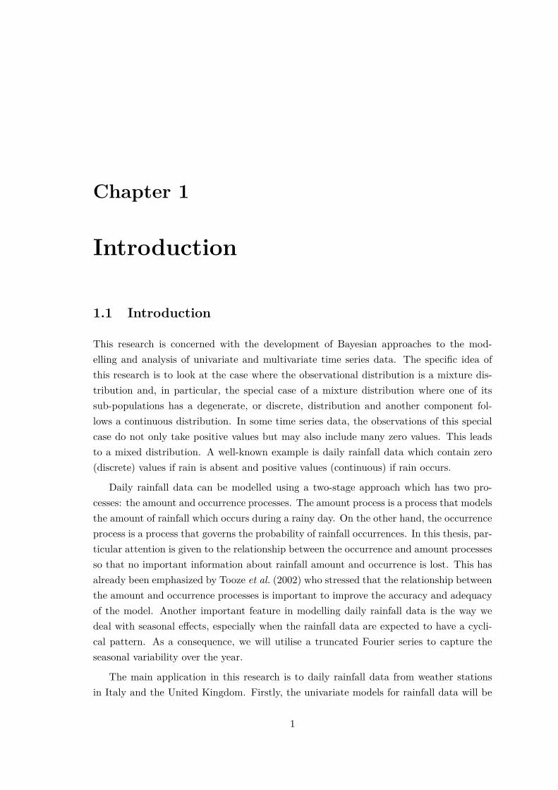
1.1 Introduction
This research is concerned with the development of Bayesian approaches to the mod-elling and analysis of univariate and multivariate time series data. The specific idea ofthis research is to look at the case where the observational distribution is a mixture dis-tribution and, in particular, the special case of a mixture distribution where one of itssub-populations has a degenerate, or discrete, distribution and another component fol-lows a continuous distribution. In some time series data, the observations of this specialcase do not only take positive values but may also include many zero values. This leadsto a mixed distribution. A well-known example is daily rainfall data which contain zero(discrete) values if rain is absent and positive values (continuous) if rain occurs.
Daily rainfall data can be modelled using a two-stage approach which has two pro-cesses: the amount and occurrence processes. The amount process is a process that modelsthe amount of rainfall which occurs during a rainy day. On the other hand, the occurrenceprocess is a process that governs the probability of rainfall occurrences. In this thesis, par-ticular attention is given to the relationship between the occurrence and amount processesso that no important information about rainfall amount and occurrence is lost. This hasalready been emphasized by Tooze et al. (2002) who stressed that the relationship betweenthe amount and occurrence processes is important to improve the accuracy and adequacyof the model. Another important feature in modelling daily rainfall data is the way wedeal with seasonal effects, especially when the rainfall data are expected to have a cycli-cal pattern. As a consequence, we will utilise a truncated Fourier series to capture theseasonal variability over the year.
The main application in this research is to daily rainfall data from weather stationsin Italy and the United Kingdom. Firstly, the univariate models for rainfall data will be
1
Chapter 1. Introduction
developed. These are then extended to multivariate models by developing spatiotemporalmodels for rainfall at several sites, with a particular attention to how the spatiotemporaldependencies affect both the occurrence and amount processes. For the British dailyrainfall application, the atmospheric circulation patterns will be directly incorporated intothe model to provide a relationship between rainfall and climate. This is in contrast withthe previous works by Heaps et al. (2015) and Germain (2010) who linked the atmosphericcirculation patterns to latent weather states to influence the daily rainfall pattern. Hence,the model for the British daily rainfall is an alternative to the models developed by Heapset al. (2015) and Germain (2010).
1.2 Research objectives
An important feature in this research is that we aim to develop and modify the work ofHeaps et al. (2015) and Germain (2010) on spatiotemporal models for daily rainfall at anetwork of weather stations. The following developments will be investigated:
1. Removing the hidden weather states from the model and using the Lamb WeatherType (LWT) as the actual weather states.
2. The modelling approach will cover rainfall data over the whole year including theseasonal effects, extending the work of Heaps et al. (2015) and Germain (2010) whoonly used the winter data in their model development. When looking at daily rainfalldata for the whole year, the transition probabilities in a Markov chain for the LWTwill depend on the particular time of year.
3. A careful examination of the conditional distribution of the rainfall amount andhow the mixed distribution of rainfall should be parameterised, how the parametersshould change under different conditions and how the dependence between sites andbetween times should be modelled in terms of these parameterisations.
The methods are illustrated using daily rainfall data from the UK and Italy.
The main objectives of this research are:
1. To investigate Bayesian time series modelling in mixed or mixture distribution ap-plications.
2. To develop novel approaches in modelling dependence, on both covariates and be-tween realisations, and how this affects both the between-component distribution(eg the occurence process in the rainfall case) and the conditional within-componentdistribution (eg for the amount process in the rainfall case).
2

Chapter 1. Introduction
3. To investigate the computation of posterior distributions in univariate and multi-variate models for mixture and mixed distributions.
4. To apply the developed methods to a number of practical problems and assess thestrengths and weaknesses of each approach.
1.3 Outline of the thesis
The structure of this thesis is organised as follows. Chapter 2 describes the general ideaof Bayesian inference and time series. We introduce some suitable models that can beused for modelling time series data. Particular attention is given to Markov chains andstate space models. The state space models can be regarded as an alternative approachto autoregressive integrated moving average (ARIMA) models in the time series context.After that, we review Bayesian inference including the use of Bayes’ theorem and someMarkov chain Monte Carlo (MCMC) techniques which include the Metropolis-Hastingsalgorithm and Gibbs sampling. The data augmentation approach is also introduced inthis chapter that can be used in the MCMC scheme to make the posterior sampling forsome models more tractable.
Chapter 3 describes the introduction of Bayesian inference in mixture models withparticular emphasis given to finite mixture models. The MCMC scheme for finite mixturemodels is then introduced with some discussion on the label switching problem. In addi-tion, we also introduce the mixed distribution which is a special case of mixture models.Using the Bayesian framework, we then develop a mixture model for some ultrasound datawith some discussion on the prior elicitation and posterior distribution.
In Chapter 4, we present the idea of modelling daily rainfall data within the Bayesianframework. We start with the general idea of how to develop a model for the amount andoccurrence processes. We then discuss the seasonal effects and their utility in capturingthe seasonal variations of daily rainfall over the year. To assess the adequacy of themodel, we introduce a diagnostic checking procedure for mixed distribution time series.For the Italian daily rainfall dataset, three different probability density functions (pdfs)are considered for modelling the amount process, and these three pdfs are subsequentlycompared by using the posterior predictive distribution. A first-order Markov chain is alsoused to model the occurrence process. For a British daily rainfall dataset, we propose analternative model to the models developed by Heaps et al. (2015) and Germain (2010).Instead of using hidden weather states, we incorporate atmospheric circulation patternsdirectly to the amount and occurrence processes. The atmospheric circulation patterns forthe British daily rainfall application are represented by the Lamb weather types (LWTs).For preliminary investigation, we will solely focus on a single site before extending the
3

Chapter 1. Introduction
work to multiple sites in Chapter 5.
Chapter 5 introduces a spatiotemporal model for the daily rainfall data at multiplesites within the United Kingdom. This model is an extended version of the univariatemodel in Chapter 4. The multivariate model is more challenging to develop than theunivariate model since it involves a large number of parameters and a high computationalcost is required to fit the model. The exploratory examination of the dataset and thesummary of investigations into the spatial and temporal characteristics of the data willalso be discussed in this chapter. The adequacy of the model will then be assessed usinga similar diagnostic checking method as introduced in Chapter 4.
Finally, Chapter 6 summarises our conclusions about the whole thesis and these includesuggestions for future work.
4
Chapter 2
Introduction to Bayesian Inferenceand Time Series
2.1 Introduction
In this chapter, we will introduce some models that are suitable to use for modelling timeseries data. We will introduce Markov chains in Section 2.2.2 and state space modelsin Section 2.2.3. The Markov chain has two different types of states: discrete (Section2.2.2.2) and continuous (Section 2.2.2.3). The state space model presents an alternativeapproach to autoregressive integrated moving average (ARIMA) models in building timeseries models. If the model is linear and the observations follow a Gaussian distribution,then we can use dynamic linear models (DLMs) to analyse the data as in Section 2.2.3.2.Alternatively, we can use dynamic generalised linear models (DGLMs) to model both non-normal and nonlinear time series (see Section 2.2.3.3). Hidden Markov models (HMMs)are another type of state space model which contain two different layers of a system: anobserved process and an unobserved process. The behaviour of the observed process can bereproduced by modelling the unobserved process as a Markov chain (see Section 2.2.3.4).
We will also describe briefly Bayesian inference including Bayes’ theorem (Section 2.3.2)and prior distributions (Section 2.3.3). After that, we will discuss the use of samplingtechniques, specifically Markov chain Monte Carlo (MCMC) to obtain posterior samplesfor parameters in Section 2.3.4. We will also introduce the data augmentation techniquein Section 2.3.5 which can be used in the MCMC scheme when the direct computation ofthe posterior samples for some models is difficult to handle. In Section 2.3.6, we reviewthe application of the Bayesian approach in time series models.
5
Chapter 2. Introduction to Bayesian Inference and Time Series
2.2 Time Series Models
2.2.1 Introduction
A time series is a collection of observations that are generated sequentially in time. Itcan also be considered as a realisation of a stochastic process. The order of a time seriesis crucial because the observations are ordered with respect to time. The applications oftime series can be found widely in various fields such as monthly rainfall, the number ofaccidents in a week, daily stock market prices, and annual series of the number of cancerpatients in a hospital. The observations of a time series are given as
y1, y2, ..., yT
where t ∈ {1, 2, · · · , T}. The observation yt is regarded as a realisation of a randomvariable Yt and can be either continuous or discrete. For the time index t, it can also havecontinuous and discrete values. However, in this thesis we only consider a discrete timeindex t, where the observations are drawn at fixed intervals.
There are some reasons why we look at time series analysis. Firstly, we want to analysethe data and describe what has happened in the past in terms of the components of interestsuch as trends, seasonal effects, patterns and fluctuations. From here, the information willbe gathered and then we will make some inferences from the data. Time series can alsobe used to assess the effects of other variables and interventions based on the behaviourof data, for example the effect of weather on gas consumption. Of course, time series canalso be used to make some predictions about the future based on the observed data.
The modelling and analysis of time series are mainly focused on two main approacheswhich are autoregressive integrated moving average (ARIMA) models (Box & Jenkins,1976) and state space models, e.g. dynamic linear models (DLMs) (West & Harrison,1997). We will use some of these approaches in our analysis. For instance, we will use thefirst order autoregressive model AR(1) for the random effect in our daily rainfall model inChapter 4. In the next section, we will review some basic theory about state space models.For an introductory survey of approaches to time series analysis, see Chatfield (2003).
2.2.2 Markov chains
2.2.2.1 Introduction
In this section, we review some basic ideas about Markov chains. A Markov chain is asequence of random variables, X(0), X(1), X(2), · · · where the future states are conditionally
6

Chapter 2. Introduction to Bayesian Inference and Time Series
independent of the past states given the present state. This process is also known as a“memoryless” process because it has no information about where it has been in the past.Beyond the present state, the process must satisfy the Markov property for all t ∈ N andthe conditional probabilities can be written as
Pr(Xt+1 = xt+1|Xt = xt, Xt−1 = xt−1, · · · , X0 = x0)
= Pr(Xt+1 = xt+1|Xt = xt). (2.1)
Figure 2.1 shows the directed acyclic graph (DAG) for the dependence structure of aMarkov chain where Xt ∈ S denotes the state of the process at time t and S is a statespace.
XtXt−1 Xt+1
Figure 2.1: A directed acyclic graph (DAG) showing the dependence structure of a Markov chain
2.2.2.2 Discrete state
When dealing with discrete state spaces, the notation for the states of a Markov chain in(2.1) can be substituted by a single letter such as i, j, k ∈ S:
Pr(Xt+1 = j|Xt = i) = pij .
The conditional probabilities for a Markov chain are known as transition probabilitiesfrom state i to state j. If we have a finite state system, that is a system with J stateswhere J <∞, then the transition matrix can be written as
P (t) =
p1,1(t) · · · p1,J(t)
... . . . ...pJ,1(t) · · · pJ,J(t)
.The elements of the matrix must satisfy these two properties:
1. 0 ≤ pij(t) ≤ 1
2.∑Jj=1 pij(t) = 1 where i, j ∈ J .
The matrix P (t) is called a Markov matrix or stochastic matrix at time t if it fulfills theseproperties. If these probabilities depend on time t, the process is called a nonhomogeneous
7
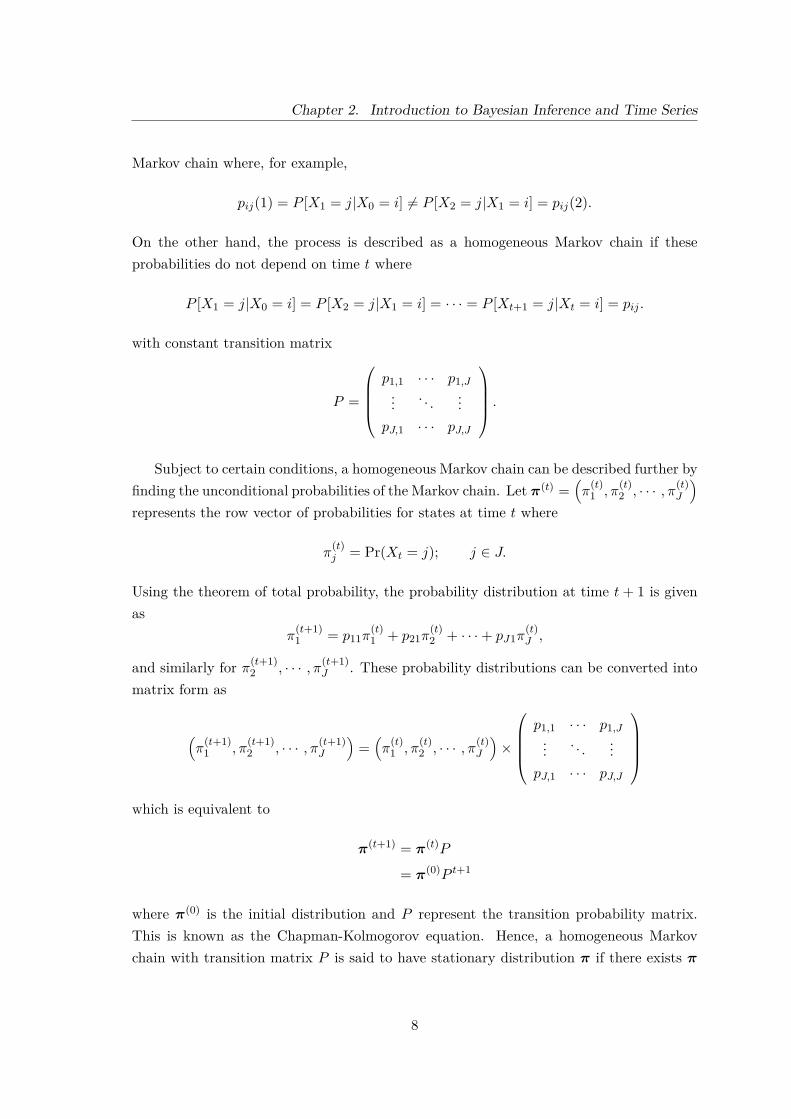
Chapter 2. Introduction to Bayesian Inference and Time Series
Markov chain where, for example,
pij(1) = P [X1 = j|X0 = i] 6= P [X2 = j|X1 = i] = pij(2).
On the other hand, the process is described as a homogeneous Markov chain if theseprobabilities do not depend on time t where
P [X1 = j|X0 = i] = P [X2 = j|X1 = i] = · · · = P [Xt+1 = j|Xt = i] = pij .
with constant transition matrix
P =
p1,1 · · · p1,J
... . . . ...pJ,1 · · · pJ,J
.
Subject to certain conditions, a homogeneous Markov chain can be described further byfinding the unconditional probabilities of the Markov chain. Let π(t) =
(π
(t)1 , π
(t)2 , · · · , π(t)
J
)represents the row vector of probabilities for states at time t where
π(t)j = Pr(Xt = j); j ∈ J.
Using the theorem of total probability, the probability distribution at time t + 1 is givenas
π(t+1)1 = p11π
(t)1 + p21π
(t)2 + · · ·+ pJ1π
(t)J ,
and similarly for π(t+1)2 , · · · , π(t+1)
J . These probability distributions can be converted intomatrix form as
(π
(t+1)1 , π
(t+1)2 , · · · , π(t+1)
J
)=(π
(t)1 , π
(t)2 , · · · , π(t)
J
)×
p1,1 · · · p1,J
... . . . ...pJ,1 · · · pJ,J
which is equivalent to
π(t+1) = π(t)P
= π(0)P t+1
where π(0) is the initial distribution and P represent the transition probability matrix.This is known as the Chapman-Kolmogorov equation. Hence, a homogeneous Markovchain with transition matrix P is said to have stationary distribution π if there exists π
8

Chapter 2. Introduction to Bayesian Inference and Time Series
such thatπ = πP
with π × 1′ = 1. It is called a stationary distribution because the distribution π(t) stays
the same as the time moves at any number k-steps:
π(t) = π(t+k) = π ∀k > 0.
Under certain conditions (see Stewart (2009)),
π(0)P t −→ π as t −→∞. (2.2)
However, in some cases, for example, P =( 0 1
1 0), (2.2) does not hold. The unconditional
probability of a homogeneous Markov chain can be found by solving
π(I − P ) = 0
where I is the J × J identity matrix. A comprehensive description of Markov chains canbe found in Zucchini (2009) and Stewart (2009).
In a hidden Markov model (see Section 2.2.3.4), the application of a Markov chainis important to model the values of the hidden process. The stationary distribution ofa Markov chain is also used in Bayesian inference to draw samples from the posteriordistribution. Markov chains are widely used in applications such as analysing rainfalloccurrence (Gabriel & Neumann, 1962), queues of customers (Kendall, 1953) and exchangerates of currencies (Masson, 2001). In the rainfall case, the homogeneous Markov chainis a favoured method to find the probability of rainfall occurrence. However, the non-homogeneous Markov chain is also employed if we believe that the probability of rainfallat time t may depend, for example, on seasonal factors. In Chapter 3, we will use bothhomogeneous and nonhomogeneous Markov chains to analyse the rainfall occurrence andthe Lamb weather types (LWTs).
2.2.2.3 Continuous state
Now, let the state space S be continuous (S ⊂ R) where the time is still discrete. For anyA ⊂ S and x ∈ S, a homogeneous chain for continuous state space is defined in a similarway to the discrete case as follows:
P (x,A) = Pr(Xt+1 ∈ A|Xt = x).
9

Chapter 2. Introduction to Bayesian Inference and Time Series
In the discrete case, this is equivalent to
P (x, x) = Pr(Xt+1 = x|Xt = x)
for x, x ∈ S. For the continuous case, we can not use this form because P (x, {x}) = 0.Instead, the notation P (x, x) can be defined as:
P (x, x) = Pr(Xt+1 ≤ x|Xt = x) = Pr(X1 ≤ x|X0 = x)
for x, x ∈ S. This form represents the transition matrix for the continuous case and theconditional density is given by
p(x, x) = ∂
∂xP (x, x)
which defines the density form of the transition kernel of the chain. Assume that theconditional transition probability moves to k-steps as follows:
P k(x, x) = Pr(Xt+k ≤ x|Xt = x),
where the transition kernel is given by
pk(x, x) = ∂
∂xP k(x, x)
for x, x ∈ S. This can be further extended by using the theorem of total probability wherethe conditional distribution at any step t+ k has the form
P t+k(x, x) =∫SP k(x, x)pt(x, x)dx
which is a continuous version of the Chapman-Kolmogorov equations. At k = 1, we have
P t+1(x, x) =∫SP (x, x)pt(x, x)dx.
Then, the marginal distribution at any time t+ 1 can be obtained as follows:
π(t+1)(x) =∫Sp(x, x)π(t)(x)dx.
A distribution π(x) on continuous state spaces is said to be a stationary distribution if itsatisfies
π(x) =∫Sp(x, x)π(x)dx.
10

Chapter 2. Introduction to Bayesian Inference and Time Series
A full comprehensive discussion about the continuous state space Markov chains can befound in Gamerman & Lopes (2006).
2.2.3 State space models
2.2.3.1 Introduction
In this section, we review some basic theory of state space models in time series analysis.State space models are an alternative to ARIMA models for constructing time series modelsand forecasting. It is a flexible model where computations for monitoring and forecastingcan be done recursively. Originally, it was developed in the engineering field for updatinginformation about the system continuously from the current position (Kalman & Bucy,1961). This is one of the reasons why the state space model literature can be found morein engineering applications. However, it is still applicable to use in many other fields suchas economics and computer sciences. For example, state space models can be used toforecast the unemployment rate as an “output” of the underlying state of the economy.This technique is also very popular among Bayesian statisticians and some of the notationsused in state space models are expressed in Bayesian terms. For instance, the expectationof future values can be considered as our belief about the future and can be updated afterwe observe the data.
The basic idea of a state space model is to have a probabilistic dependence betweenthe observation, Yt and an unobserved state variable Xt:
Yt = h(Xt) + ηt
where h(.) is some function. Often h(.) is a linear function that contains a linear com-bination of several components such as trend, seasonal or regressive components. Theunobserved state variable Xt is also known as the signal and the random variable ηt iscalled the noise. In most cases, ηt is assumed to be independent from ηs when s 6= t.Therefore Yt is conditionally independent of Ys given Xt where s 6= t. The observations Ytcan be either univariate or multivariate. Typically, the sequence {Xt} is a Markov chain.In this case, in terms of the joint probability density, the state space model can be writtenas
π(x1:T , y1:T ) =π(x1)π(x2|x1)π(x3|x2) · · · × π(y1|x1)π(y2|x2)π(y3|x3) · · ·
= π(x1)π(y1|x1)T∏t=2
[π(xt|xt−1)π(yt|xt)]
where the conditional distributions often stay the same over time. By introducing the
11
Chapter 2. Introduction to Bayesian Inference and Time Series
initial distribution π(x0), the state space model can be simplified to
π(x0:T , y1:T ) = π(x0)T∏t=1
[π(xt|xt−1)π(yt|xt)] . (2.3)
The state space model can help to solve a broad range of time series problems such asinference for unknown parameters, smoothing and prediction. For details, see Kitagawa(1998), Durbin & Koopman (2000), and Christensen et al. (2012). It is considered to beone of the best approaches in time series at handling missing values. A particular exampleof a state space model in time series is a hidden Markov model. We will discuss hiddenMarkov models in Section 2.2.3.4. In addition, the parameterisation of ARIMA modelscan be converted into state space form.
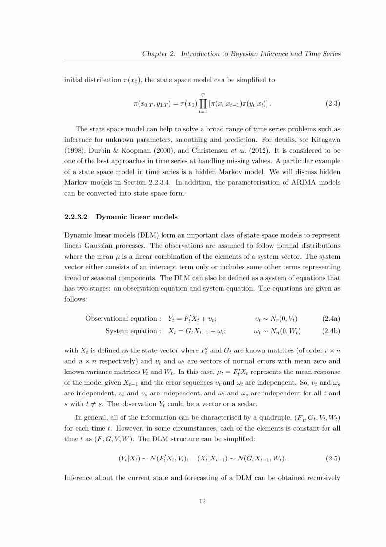
2.2.3.2 Dynamic linear models
Dynamic linear models (DLM) form an important class of state space models to representlinear Gaussian processes. The observations are assumed to follow normal distributionswhere the mean µ is a linear combination of the elements of a system vector. The systemvector either consists of an intercept term only or includes some other terms representingtrend or seasonal components. The DLM can also be defined as a system of equations thathas two stages: an observation equation and system equation. The equations are given asfollows:
Observational equation : Yt = F ′tXt + υt; υt ∼ Nr(0, Vt) (2.4a)
System equation : Xt = GtXt−1 + ωt; ωt ∼ Nn(0,Wt) (2.4b)
with Xt is defined as the state vector where F ′t and Gt are known matrices (of order r×nand n × n respectively) and υt and ωt are vectors of normal errors with mean zero andknown variance matrices Vt and Wt. In this case, µt = F ′tXt represents the mean responseof the model given Xt−1 and the error sequences υt and ωt are independent. So, υt and ωsare independent, υt and υs are independent, and ωt and ωs are independent for all t ands with t 6= s. The observation Yt could be a vector or a scalar.
In general, all of the information can be characterised by a quadruple, (F t, Gt, Vt,Wt)for each time t. However, in some circumstances, each of the elements is constant for alltime t as (F ,G, V,W ). The DLM structure can be simplified:
(Yt|Xt) ∼ N(F ′tXt, Vt); (Xt|Xt−1) ∼ N(GtXt−1,Wt). (2.5)
Inference about the current state and forecasting of a DLM can be obtained recursively
12
Chapter 2. Introduction to Bayesian Inference and Time Series
by using the Kalman filter. Detailed explanations and examples of DLM can be found inWest & Harrison (1997) and Petris et al. (2009).
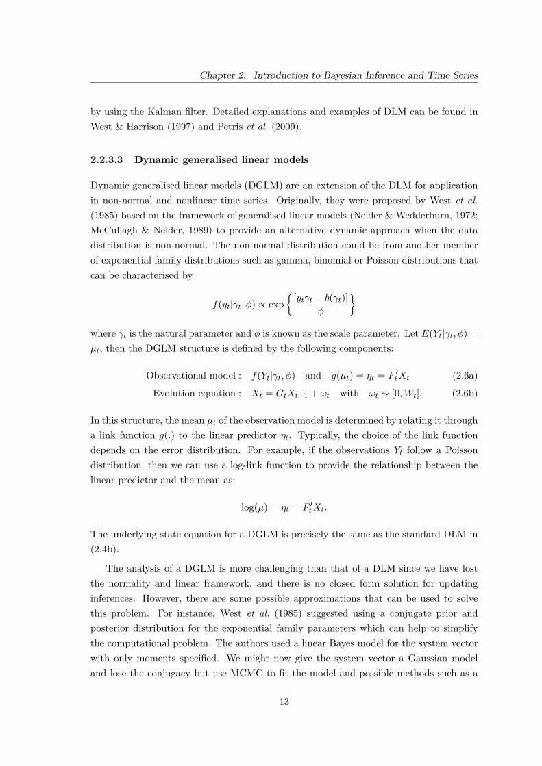
2.2.3.3 Dynamic generalised linear models
Dynamic generalised linear models (DGLM) are an extension of the DLM for applicationin non-normal and nonlinear time series. Originally, they were proposed by West et al.(1985) based on the framework of generalised linear models (Nelder & Wedderburn, 1972;McCullagh & Nelder, 1989) to provide an alternative dynamic approach when the datadistribution is non-normal. The non-normal distribution could be from another memberof exponential family distributions such as gamma, binomial or Poisson distributions thatcan be characterised by
f(yt|γt, φ) ∝ exp{ [ytγt − b(γt)]
φ
}where γt is the natural parameter and φ is known as the scale parameter. Let E(Yt|γt, φ) =µt, then the DGLM structure is defined by the following components:
Observational model : f(Yt|γt, φ) and g(µt) = ηt = F ′tXt (2.6a)
Evolution equation : Xt = GtXt−1 + ωt with ωt ∼ [0,Wt]. (2.6b)
In this structure, the mean µt of the observation model is determined by relating it througha link function g(.) to the linear predictor ηt. Typically, the choice of the link functiondepends on the error distribution. For example, if the observations Yt follow a Poissondistribution, then we can use a log-link function to provide the relationship between thelinear predictor and the mean as:
log(µ) = ηt = F ′tXt.
The underlying state equation for a DGLM is precisely the same as the standard DLM in(2.4b).
The analysis of a DGLM is more challenging than that of a DLM since we have lostthe normality and linear framework, and there is no closed form solution for updatinginferences. However, there are some possible approximations that can be used to solvethis problem. For instance, West et al. (1985) suggested using a conjugate prior andposterior distribution for the exponential family parameters which can help to simplifythe computational problem. The authors used a linear Bayes model for the system vectorwith only moments specified. We might now give the system vector a Gaussian modeland lose the conjugacy but use MCMC to fit the model and possible methods such as a
13
Chapter 2. Introduction to Bayesian Inference and Time Series
particle filter for filtering. The full comprehensive development of DGLMs can found inWest et al. (1985) and West & Harrison (1997).
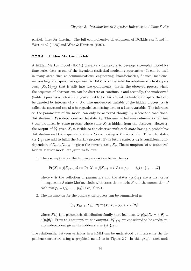
2.2.3.4 Hidden Markov models
A hidden Markov model (HMM) presents a framework to develop a complex model fortime series data as one of the ingenious statistical modelling approaches. It can be usedin many areas such as communications, engineering, bioinformatics, finance, medicine,meteorology and speech recognition. A HMM is a bivariate discrete-time stochastic pro-cess, {Xt,Yt}t≥1 that is split into two components: firstly, the observed process wherethe sequence of observations can be discrete or continuous and secondly, the unobserved(hidden) process which is usually assumed to be discrete with a finite state space that canbe denoted by integers {1, · · · , J}. The unobserved variable of the hidden process, Xt iscalled the state and can also be regarded as missing data or a latent variable. The inferenceon the parameters of the model can only be achieved through Yt where the conditionaldistribution of Yt is dependent on the state Xt. This means that every observation at timet was produced by some process whose state Xt is hidden from the observer. However,the output of Yt given Xt is visible to the observer with each state having a probabilitydistribution and the sequence of states Xt comprising a Markov chain. Then, the states{Xt}t≥1 are said to fulfill the Markov property if the future state, Xt+1 is conditionally in-dependent of Xt−1, Xt−2, · · · given the current state, Xt. The assumptions of a “standard”hidden Markov model are given as follows:
1. The assumption for the hidden process can be written as
Pr(Xt = j|X1:t−1,θ) = Pr(Xt = j|Xt−1 = i, P ) = pij i, j ∈ {1, · · · , J}
where θ is the collection of parameters and the states {Xt}t≥1 are a first orderhomogeneous J-state Markov chain with transition matrix P and the summation ofeach row pi = (pi1, · · · , pij) is equal to 1.
2. The assumption for the observation process can be summarised as
(Yt|Y1:t−1, X1:T ,θ) ≡ (Yt|Xt = j,θ) ∼ F(θj)
where F(.) is a parametric distribution family that has density p(yt|Xt = j,θ) ≡p(yt|θj). From this assumption, the outputs {Yt}t≥1 are considered to be condition-ally independent given the hidden states {Xt}t≥1.
The relationship between variables in a HMM can be understood by illustrating the de-pendence structure using a graphical model as in Figure 2.2. In this graph, each node
14

Chapter 2. Introduction to Bayesian Inference and Time Series
XtXt−1 Xt+1
YtYt−1 Yt+1
Figure 2.2: A DAG showing the dependence structure of a “standard” hidden Markov model
represents a random variable. The arrows correspond to the structure of the joint proba-bility distribution. A hidden Markov model is said to be homogeneous when the transitionprobabilities of the Markov chain for the underlying process are constant over time andthe conditional distributions of Yt|Xt remain constant over time.
There are a few extensions for HMM which have been reviewed by Germain (2010)and Cappe et al. (2005). For example, the order of the Markov chain for the hiddenprocess can be more than one. Let the hidden state sequence {Xt}t≥1 be a d-th orderMarkov process. Then, we can say that the conditional distribution of the future state,Xt+1 depends on the previous d values, Xt−d, Xt−d+1, · · · , Xt−1. Conceptually, modelswith d > 1 are as straightforward as in a standard hidden Markov model but we willnot consider this case in our study. The hidden Markov model can be further extendedby allowing the model to have non-homogeneous transition probabilities for the hiddenprocess or non-homogeneous observation distributions for the observation process. Then,we can say that the distribution of Xt+1 given Xt or Yt given Xt is changed for everytime-step t.
2.2.3.5 Markov switching models
A notable generalisation for hidden Markov models is Markov switching models. Forthis generalisation, the observed process allows the conditional distribution of Yt+1 giventhe history of past variables to depend not only on Xt+1 but also on the previous qobservations, Yt−q,Yt−q+1, · · · ,Yt−1. The dependence structure of this model is illustratedas in Figure 2.3. The statistical analysis for a Markov switching model is more complicatedthan for a HMM since Yt does not simply depend on Xt only but also on Yt−q, · · · ,Yt−1.
15

Chapter 2. Introduction to Bayesian Inference and Time Series
XtXt−1 Xt+1
YtYt−1 Yt+1
Figure 2.3: A DAG showing the dependence structure of Markov switching model with q = 1
2.3 Bayesian Inference
2.3.1 Introduction
In the Bayesian framework, probability distributions are used to describe uncertaintyabout the values of unknown quantities, whether these are parameters, missing data,latent variables or future observations. This is in contrast with the frequentist approachwhere, for example, the value of a parameter is regarded as fixed but unknown and nodistinction is made between possible values which are more or less likely.
In Bayesian inference, the distribution given to the value of an unknown quantitybefore data are observed is called a prior distribution. When data are observed, thelikelihood function from these data is combined with the prior distribution to give aposterior distribution which describes the new state of uncertainty about the value of theunknown quantity. The information from the posterior distribution can be summarised tomake statistical inferences.
2.3.2 Bayes’ theorem
Bayes’ theorem or Bayes’ rule plays a central role in Bayesian inference where it combinesprior belief with observed data to obtain the conditional probability of a given hypothesis.Let A1, A2, ..., An be a set of mutually exclusive events that form the sample space S.Given an additional event B from the same sample space with Pr(B) > 0, Bayes’ theoremcan be written as:
Pr(Aj |B) = Pr(Aj ∩B)Pr(A1 ∩B) + Pr(A2 ∩B) + ...+ Pr(An ∩B) = Pr(Aj ∩B)∑n
i=1 Pr(Ai ∩B)
16

Chapter 2. Introduction to Bayesian Inference and Time Series
Using the fact that Pr(Aj ∩B) = Pr(Aj) Pr(B|Aj), Bayes’ theorem can then be rewrittenas:
Pr(Aj |B) = Pr(Aj) Pr(B|Aj)∑ni=1 Pr(Ai) Pr(B|Ai)
Suppose we have a set of observations y=(y1, y2, ..., yn) which depend on a set of k unknownquantities, θ = (θ1, θ2, ..., θk) and we are interested in making inference about θ. Thelikelihood of parameter θ can be expressed as
L(θ|y) = f(y|θ).
If y1, · · · , yn are conditionally independent given θ, then we can write
L(θ|y) =n∏i=1
fi(yi|θ).
The prior beliefs for θ can be represented as a probability density or probability massfunction, π(θ). Hence, we can summarise our beliefs about θ using information fromthe prior and this is subsequently updated by the likelihood, resulting in a posteriordistribution, π(θ|y). Using Bayes’ theorem, the posterior density π(θ|y) can be expressedas:
π(θ|y) = π(θ)f(y|θ)f(y) (2.7)
where
f(y) =
∫Θ π(θ)f(y|θ)dθ if θ is continuous
∑Θ π(θ)f(y|θ) if θ is discrete
and Θ is the set of possible values of θ. From (2.7), f(y) is a normalising constant ormarginal likelihood of the data which ensures that the posterior density always integratesto one (if continuous) or sums to one (if discrete). Since this is not a function of θ, thenthe posterior distribution can be simplified as
π(θ|y) ∝ π(θ)× f(y|θ) (2.8)
that isPosterior ∝ Prior × Likelihood.
In many cases, the normalising constant p(y) is not available in analytical closed form.Numerical integration or analytic approximation is hence required to solve the difficultyof not having a closed form especially when we have an integral for continuous unknowns.There are several techniques that can be used to solve this problem but the most popularone is known as Markov Chain Monte Carlo (MCMC) which generates samples of the
17
Chapter 2. Introduction to Bayesian Inference and Time Series
values of parameters from the posterior distribution in complex models without computingthe integral for the normalising constant f(y) in Bayes’ rule. As this technique is easierand more practical to use, MCMC techniques will be used for analysis in this study.
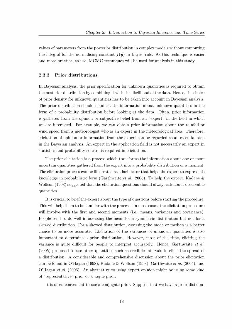
2.3.3 Prior distributions
In Bayesian analysis, the prior specification for unknown quantities is required to obtainthe posterior distribution by combining it with the likelihood of the data. Hence, the choiceof prior density for unknown quantities has to be taken into account in Bayesian analysis.The prior distribution should manifest the information about unknown quantities in theform of a probability distribution before looking at the data. Often, prior informationis gathered from the opinion or subjective belief from an “expert” in the field in whichwe are interested. For example, we can obtain prior information about the rainfall orwind speed from a meteorologist who is an expert in the meteorological area. Therefore,elicitation of opinion or information from the expert can be regarded as an essential stepin the Bayesian analysis. An expert in the application field is not necessarily an expert instatistics and probability so care is required in elicitation.
The prior elicitation is a process which transforms the information about one or moreuncertain quantities gathered from the expert into a probability distribution or a moment.The elicitation process can be illustrated as a facilitator that helps the expert to express hisknowledge in probabilistic form (Garthwaite et al., 2005). To help the expert, Kadane &Wolfson (1998) suggested that the elicitation questions should always ask about observablequantities.
It is crucial to brief the expert about the type of questions before starting the procedure.This will help them to be familiar with the process. In most cases, the elicitation procedurewill involve with the first and second moments (i.e. means, variances and covariance).People tend to do well in assessing the mean for a symmetric distribution but not for askewed distribution. For a skewed distribution, assessing the mode or median is a betterchoice to be more accurate. Elicitation of the variances of unknown quantities is alsoimportant to determine a prior distribution. However, most of the time, eliciting thevariance is quite difficult for people to interpret accurately. Hence, Garthwaite et al.(2005) proposed to use other quantities such as credible intervals to elicit the spread ofa distribution. A considerable and comprehensive discussion about the prior elicitationcan be found in O’Hagan (1998), Kadane & Wolfson (1998), Garthwaite et al. (2005), andO’Hagan et al. (2006). An alternative to using expert opinion might be using some kindof “representative” prior or a vague prior.
It is often convenient to use a conjugate prior. Suppose that we have a prior distribu-
18
Chapter 2. Introduction to Bayesian Inference and Time Series
tion for θ that has probability density function π(θ). When we have observed data, thelikelihood function is given as L(θ|y). By combining the prior distribution and likelihood,we can obtain the posterior distribution as
π(θ|y) ∝ π(θ)L(θ|y).
If π(θ) and π(θ|y) belong to the same family of distributions, then π(θ) is said to be aconjugate prior distribution. The form of the conjugate prior relies closely on the form ofthe likelihood. Hence we will have a different conjugate distribution if we have a differentdata distribution. Prior beliefs might not always be well represented by a conjugatedistribution. However, sometimes a conjugate prior will represent prior beliefs sufficientlyclosely and this will help to make the calculations easier.
2.3.4 Markov Chain Monte Carlo (MCMC) methods
2.3.4.1 Introduction
In Bayesian analysis, computing the posterior density is relatively straightforward whenwe use a conjugate prior. However, it may become difficult if the distributions are complexand analytically intractable especially in higher dimensions. Markov chain Monte Carlo(MCMC) is a technique to tackle this problem by drawing samples from the complexposterior distributions without computing the integral in Bayes’ rule. The basic idea ofMCMC techniques is to construct a Markov chain which has the posterior distribution asits stationary distribution. Then, by generating a realisation of the Markov chain for asufficiently long number of steps and provided that the chain has converged, the sampleswill be generated from the posterior distribution. The introduction of MCMC gives analternative for us to make any inference of interest by generating the whole distributionnumerically. For comprehensive theory, developments and applications of MCMC, thereader can refer to Besag et al. (1995), Gamerman (1997), Brooks & Gelman (1998),Gamerman & Lopes (2006) and Brooks et al. (2011). In the following sections, we willbriefly define two fundamental MCMC techniques: the Gibbs sampler and Metropolis-Hastings algorithms, to generate samples from posterior distributions.
2.3.4.2 Metropolis-Hastings Algorithm
The Metropolis algorithm was developed by Metropolis et al. (1953) before it was gen-eralised by Hastings (1970) to be the Metropolis-Hastings algorithm. Suppose we areinterested in sampling realisations from the posterior distribution π(θ|y) which has a non-standard form. By introducing a proposal distribution with density q(θ∗|θ), it makes
19
Chapter 2. Introduction to Bayesian Inference and Time Series
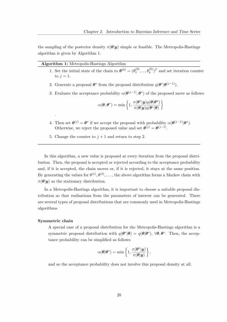
the sampling of the posterior density π(θ|y) simple or feasible. The Metropolis-Hastingsalgorithm is given by Algorithm 1.
Algorithm 1: Metropolis-Hastings Algorithm1. Set the initial state of the chain to θ(0) = (θ(0)
1 , ..., θ(0)k )T and set iteration counter
to j = 1.
2. Generate a proposal θ∗ from the proposal distribution q(θ∗|θ(j−1)).
3. Evaluate the acceptance probability α(θ(j−1),θ∗) of the proposed move as follows:
α(θ,θ∗) = min{
1, π(θ∗|y)q(θ|θ∗)π(θ|y)q(θ∗|θ)
}.
4. Then set θ(j) = θ∗ if we accept the proposal with probability α(θ(j−1)|θ∗).Otherwise, we reject the proposed value and set θ(j) = θ(j−1).
5. Change the counter to j + 1 and return to step 2.
In this algorithm, a new value is proposed at every iteration from the proposal distri-bution. Then, the proposal is accepted or rejected according to the acceptance probabilityand, if it is accepted, the chain moves or, if it is rejected, it stays at the same position.By generating the values for θ(1), θ(2), . . . , the above algorithm forms a Markov chain withπ(θ|y) as the stationary distribution.
In a Metropolis-Hastings algorithm, it is important to choose a suitable proposal dis-tribution so that realisations from the parameters of interest can be generated. Thereare several types of proposal distributions that are commonly used in Metropolis-Hastingsalgorithms.
Symmetric chainA special case of a proposal distribution for the Metropolis-Hastings algorithm is asymmetric proposal distribution with q(θ∗|θ) = q(θ|θ∗), ∀θ,θ∗. Then, the accep-tance probability can be simplified as follows:
α(θ|θ∗) = min{
1, π(θ∗|y)π(θ|y)
},
and so the acceptance probability does not involve this proposal density at all.
20
Chapter 2. Introduction to Bayesian Inference and Time Series
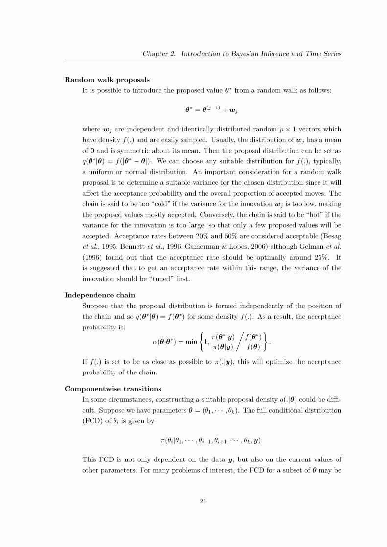
Random walk proposalsIt is possible to introduce the proposed value θ∗ from a random walk as follows:
θ∗ = θ(j−1) +wj
where wj are independent and identically distributed random p × 1 vectors whichhave density f(.) and are easily sampled. Usually, the distribution of wj has a meanof 0 and is symmetric about its mean. Then the proposal distribution can be set asq(θ∗|θ) = f(|θ∗ − θ|). We can choose any suitable distribution for f(.), typically,a uniform or normal distribution. An important consideration for a random walkproposal is to determine a suitable variance for the chosen distribution since it willaffect the acceptance probability and the overall proportion of accepted moves. Thechain is said to be too “cold” if the variance for the innovation wj is too low, makingthe proposed values mostly accepted. Conversely, the chain is said to be “hot” if thevariance for the innovation is too large, so that only a few proposed values will beaccepted. Acceptance rates between 20% and 50% are considered acceptable (Besaget al., 1995; Bennett et al., 1996; Gamerman & Lopes, 2006) although Gelman et al.(1996) found out that the acceptance rate should be optimally around 25%. Itis suggested that to get an acceptance rate within this range, the variance of theinnovation should be “tuned” first.
Independence chainSuppose that the proposal distribution is formed independently of the position ofthe chain and so q(θ∗|θ) = f(θ∗) for some density f(.). As a result, the acceptanceprobability is:
α(θ|θ∗) = min{
1, π(θ∗|y)π(θ|y)
/f(θ∗)f(θ)
}.
If f(.) is set to be as close as possible to π(.|y), this will optimize the acceptanceprobability of the chain.
Componentwise transitionsIn some circumstances, constructing a suitable proposal density q(.|θ) could be diffi-cult. Suppose we have parameters θ = (θ1, · · · , θk). The full conditional distribution(FCD) of θi is given by
π(θi|θ1, · · · , θi−1, θi+1, · · · , θk,y).
This FCD is not only dependent on the data y, but also on the current values ofother parameters. For many problems of interest, the FCD for a subset of θ may be
21

Chapter 2. Introduction to Bayesian Inference and Time Series
suitable for sampling. Let the FCD for the ith component of θ be denoted by
π(θi | θ1, . . . , θi−1, θi+1, . . . , θk,y) = π(θi | θ−i,y); i = 1, · · · , k.
The algorithm for componentwise transitions is given by Algorithm 2.
Algorithm 2: Metropolis-Hastings: Componentwise Transitions1. Set the initial state of the chain to θ(0) = (θ(0)
1 , ..., θ(0)k )T and set the iteration
counter to j = 1.2. For every iteration j, we obtain a new value of θ(j) from θ(j−1) by successive
generation from distributions:
• θ(j)1 ∼ π(θ1|θ(j−1)
2 , θ(j−1)3 , ..., θ
(j−1)k ,y) using a Metropolis-Hastings step with
proposal distribution q1(θ∗1|θ(j−1)1 )
• θ(j)2 ∼ π(θ2|θ(j)
1 , θ(j−1)3 , ..., θ
(j−1)k ,y) using a Metropolis-Hastings step with
proposal distribution q2(θ∗2|θ(j−1)2 )
...• θ(j)
k ∼ π(θk|θ(j)1 , θ
(j)2 , ..., θ
(j)k−1,y) using a Metropolis-Hastings step with proposal
distribution qk(θ∗k|θ(j−1)k ).
3. Change the iteration counter from j to j + 1 and return to step 2.
This is in fact the original form of the Metropolis algorithm where the Metropolis-Hastings algorithm presented in Algorithm 1 can be regarded as a special case ofthis algorithm. If the full conditional distribution for the particular component θi isavailable for sampling directly, then it is easy to show that the resulting acceptanceprobability is one. For this reason, this algorithm can also be called Metropolis-within-Gibbs. When all full conditional distributions are completely known andavailable for sampling from, then we can obtain an algorithm known as the Gibbssampler which is presented in the next section.
2.3.4.3 Gibbs Sampler
The Gibbs sampler was originally developed by Geman & Geman (1984) for image pro-cessing before Gelfand & Smith (1990) brought this approach to the larger statisticalcommunity (Gamerman & Lopes, 2006). Suppose we have a posterior density π(θ|y),where θ = (θ1, θ2, ..., θk)T . To generate realisations from this posterior density, samplesare drawn from full conditional distributions, with densities
π(θi|θ1, ..., θi−1, θi+1..., θk,y) = π(θi|.), i = 1, 2, ..., k.
22
Chapter 2. Introduction to Bayesian Inference and Time Series
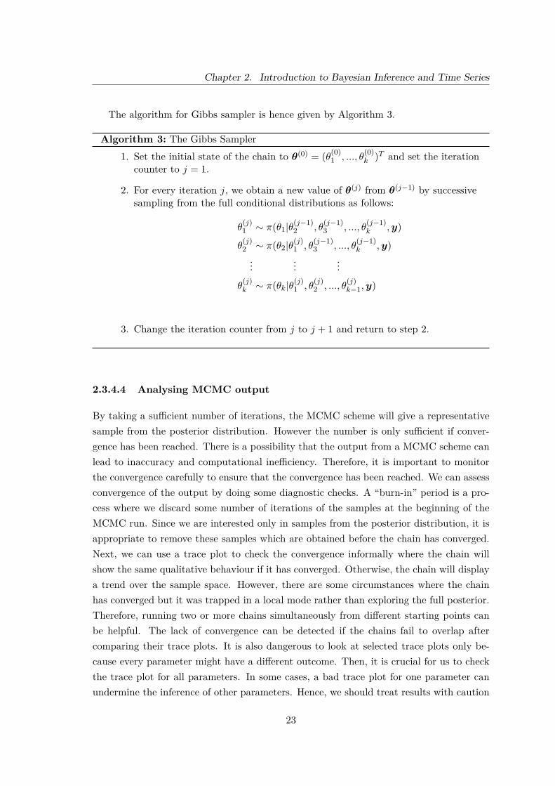
The algorithm for Gibbs sampler is hence given by Algorithm 3.
Algorithm 3: The Gibbs Sampler1. Set the initial state of the chain to θ(0) = (θ(0)
1 , ..., θ(0)k )T and set the iteration
counter to j = 1.
2. For every iteration j, we obtain a new value of θ(j) from θ(j−1) by successivesampling from the full conditional distributions as follows:
θ(j)1 ∼ π(θ1|θ(j−1)
2 , θ(j−1)3 , ..., θ
(j−1)k ,y)
θ(j)2 ∼ π(θ2|θ(j)
1 , θ(j−1)3 , ..., θ
(j−1)k ,y)
......
...
θ(j)k ∼ π(θk|θ
(j)1 , θ
(j)2 , ..., θ
(j)k−1,y)
3. Change the iteration counter from j to j + 1 and return to step 2.
2.3.4.4 Analysing MCMC output
By taking a sufficient number of iterations, the MCMC scheme will give a representativesample from the posterior distribution. However the number is only sufficient if conver-gence has been reached. There is a possibility that the output from a MCMC scheme canlead to inaccuracy and computational inefficiency. Therefore, it is important to monitorthe convergence carefully to ensure that the convergence has been reached. We can assessconvergence of the output by doing some diagnostic checks. A “burn-in” period is a pro-cess where we discard some number of iterations of the samples at the beginning of theMCMC run. Since we are interested only in samples from the posterior distribution, it isappropriate to remove these samples which are obtained before the chain has converged.Next, we can use a trace plot to check the convergence informally where the chain willshow the same qualitative behaviour if it has converged. Otherwise, the chain will displaya trend over the sample space. However, there are some circumstances where the chainhas converged but it was trapped in a local mode rather than exploring the full posterior.Therefore, running two or more chains simultaneously from different starting points canbe helpful. The lack of convergence can be detected if the chains fail to overlap aftercomparing their trace plots. It is also dangerous to look at selected trace plots only be-cause every parameter might have a different outcome. Then, it is crucial for us to checkthe trace plot for all parameters. In some cases, a bad trace plot for one parameter canundermine the inference of other parameters. Hence, we should treat results with caution
23

Chapter 2. Introduction to Bayesian Inference and Time Series
if there is evidence of non-convergence in any of the trace plots. There are also variousformal diagnostic checks available such as those recommended by Heidelberger & Welch(1983), Geweke (1992), Raftery & Lewis (1992) and Gelman & Rubin (1992) and thesehad been thoroughly reviewed by Cowles & Carlin (1996).
Apart from that, we can also use kernel density plots to identify multimodality in theposterior distribution. If multimodality of the marginal posterior is detected, then we mayneed to take an action by running the MCMC algorithm longer to ensure that the entiresample space is covered adequately.
Samples of the MCMC scheme will be dependent, meaning successive draws are au-tocorrelated. This can be observed by looking at an autocorrelation plot. When thereis little dependence between successive samples, the chain is said to mix well. If there isstrong correlation between successive values in the chain, it will take longer to explore theentire region of the parameter space which is described as poor mixing in the chain.
In general, the distribution of the chain θ(i)|y tends to the posterior distribution θ|yby increasing the number of iterations until convergence is reached.
2.3.5 Data augmentation
In some circumstances, the direct computation of the posterior density for some modelsis difficult to handle because it is laborious to compute the likelihood. In some cases,it is possible to simplify this problem by using data augmentation. Data augmentationis a common approach in Bayesian statistics to construct an iterative algorithm for theposterior sampling by introducing unobservable variables, known as auxiliary variables. Ifthese variables were observed, then the computation of the posterior density would becomestraightforward. This approach was demonstrated by Tanner & Wong (1987) and MCMCmethods are well suited to this approach.
Suppose we have observed data, y from a distribution which is conditional on theparameter vector, θ. The idea of this approach is to augment y with the auxiliary data,z. Thus, the posterior density is given as follows:
π(θ|y) =∫π(θ|y, z)π(z|y)dz (2.9)
whereπ(z|y) =
∫π(z|θ,y)π(θ|y)dθ. (2.10)
Tanner & Wong (1987) then introduced an iterative sampling scheme to construct approx-imations for π(θ|y) and π(z|y) using two steps:
24
Chapter 2. Introduction to Bayesian Inference and Time Series
1. draw samples for z using π(z|θ,y),
2. then, based on z, draw samples for θ using π(θ|y, z).
The first step is known as “imputation” step and the later is called “posterior” step.Often, the data augmentation is used to handle missing data using an MCMC scheme. Itcan also be applied in mixture distributions by introducing a group-membership variablewhich is unobserved. In this case, z can be expressed as the component of the mixturewhich generates the observed data. If z is known, then the computational analysis becomesimpler by considering that zi = j, where j ∈ {1, · · · , J} is a component of the mixturedistribution. This will be discussed in Chapter 3, Section 3.2.
2.3.6 Bayesian inference for time series models
In time series analysis, the Bayesian approach can provide a systematic framework whichoffers a complete way to analyse data by combining the prior information with the data.Then, Bayesian analysis can be applied to various types of time series models. For instance,a Bayesian approach can be used to analyse the uncertainty of missing values in thesequence of any observations. Kong et al. (1994) showed that the posterior distribution formissing data could be generated by applying the data augmentation and a Gibbs samplerto the model. Originally, the Bayesian approach was not very popular in time seriesanalysis since it is analytically intractable especially when the conjugate distributions donot represent the prior distribution of the parameters. However, this difficulty has beenresolved in the 1990s due to more advanced computing power and the introduction ofMCMC for sampling from Bayesian posterior distributions. Some of the Bayesian methodsto compute the posterior distribution have already been discussed in Section 2.3.4.
Traditionally, the DLM approach tends to be favoured by Bayesian statisticians formodelling time series, probably for historical reasons (see Harrison & Stevens (1971) andWest & Harrison (1997)). The DLM approach is more easily described in Bayesian terms.For instance, our beliefs about the future can be represented by the expectation of futurevalues and can be updated when we observe data. The Bayesian approach can also beextended to other types of state space model such as DGLM (see West et al. (1985)) andHMM (see Scott (2002)). Consider a DGLM where the observational distribution at timet has a density fy (yt|µt, φ), where φ is a scale parameter and µt is a location parameter.Let ηt = g(µt) = F
′tXt and the evolution is given in (2.6b). Using the ideas of data
augmentation, as in Section 2.3.5, the full-data likelihood is
f0(X0)T∏t=1
fY (yt|µt, φ)fX(Xt|Xt−1).
25

Chapter 2. Introduction to Bayesian Inference and Time Series
The system vectors X0, X1, · · · , XT are unobserved and can be treated as auxiliary datain an MCMC scheme.
However, there is no reason why Bayesians can not use other models in time seriessuch as ARMA models. A considerable amount of early literature has been publishedon ARMA models within a Bayesian framework, for example, Zellner (1971), Harrison& Stevens (1976), and Monahan (1983). The ARMA models can also be found in someapplication of microeconomics time series such as unemployment rates using Bayesianapproach (de Alba, 1993; Rosenberg & Young, 1999). Thus, there is strong evidence thatthe Bayesian approach can be applied to any time series models.
2.4 Conclusion
This chapter has briefly discussed the general approaches in time series models andBayesian inference. We have presented a simple discussion in Section 2.3.6 about theapplication of Bayesian approach in time series models. There are a few time series meth-ods that we will apply to build a daily rainfall model within the Bayesian framework. Itis important to introduce some of the preliminary ideas that we will use in this study. Wehave also emphasised the use of MCMC techniques to generate posterior samples for theunknown parameters. Next, we will discuss the application of the Bayesian approach in amixture model.
26

Chapter 3
Introduction to Bayesian inferencein mixture models
3.1 Introduction
Mixture models were introduced by Newcomb (1886) and Pearson (1894) as a tool forstatistical modelling. There are two main reasons why we want to use a mixture modelas a sampling distribution. Firstly, we believe that there are two or more sub-populationsand it is therefore reasonable to represent them as mixture components. For example, thesize of starlings might be different for resident birds and migrants. Thus, it is sensible toassume that there are two sub-populations of starlings in the samples. Secondly, a mixturedistribution gives greater flexibility in the sampling model and the shape of the distributionin spite of not having the “physical” interpretation for the mixture components.
In this chapter we will review the application of Bayesian inference in mixture mod-els, focusing on finite mixtures. The form of the likelihood for the finite mixture modelwill be discussed in Section 3.2. Section 3.3 illustrates the construction of Monte CarloMarkov Chain (MCMC) schemes for the finite mixture model with discussions on the labelswitching problem. We will discuss the special case of mixture models which is also knownas a mixed distribution in Section 3.4. The observations in this model type contain bothdiscrete and continuous components for example zero values and positive values. Then, wewill apply the developed mixture models to data on ultrasound measurements within theBayesian framework in Section 3.5. In this section, two types of mixture models will beconsidered in this application. The construction of the prior distribution and the resultingposterior distribution for both models will also be discussed in this section.
27
Chapter 3. Introduction to Bayesian inference in mixture models
3.2 Finite mixture model
In general, the distribution of Yi given the parameter θj is called a finite mixture model ifthe probability density function of Yi is
f(yi|π,θ) =J∑j=1
πjfj(yi|θj) (3.1)
where∑Jj=1 πj = 1 and πj ≥ 0 is the probability of each component j membership
with J as the number of components. Then, if we have independent observations y =(y1, y2, · · · , yn)T , the likelihood for the mixture model can be written as:
f(y|π,θ) =n∏i=1
J∑j=1
πjfj(yi|θj)
(3.2)
which is known as the observed data likelihood.
For instance, suppose that we have a simple two-component mixture model. Then thedensity of Yi is given as:
f(yi|π, θ1, θ2) = πf1(yi|θ1) + (1− π)f2(yi|θ2)
where fj(y|θj) is the density for component j which depends on parameters θj . In thismodel, the probability for the first component is represented by π and the probabilityof second component is (1 − π), with 0 ≤ π ≤ 1. Thus, the likelihood of independentobservations y is given as:
f(y|π, θ1, θ2) =n∏i=1
[πf1(yi|θ1) + (1− π)f2(yi|θ2)].
However, if we have more than two components, the likelihood in (3.2) could be verycomplicated. One way to simplify inference for this model is by using data augmentation(Tanner & Wong, 1987). Using this approach, we can introduce a group-membershipvariable for mixture components which is unobserved. Suppose that we have a set ofauxiliary variables z = (z1, · · · , zn)T which corresponds to the unknown component ofmixture with zi ∈ {1, · · · , J}. Given zi = j, the conditional likelihood can be written as
f(y|z,π,θ) =n∏i=1
fzi(yi|θzi).
If z is known, the conditional density for yi can thus be simplified as fzi(yi|θi). Given the
28

Chapter 3. Introduction to Bayesian inference in mixture models
probability of each unknown component of mixture, Pr(zi = j) = πj , the variables z havea multinomial or categorical distribution. Then, by observing y and z, the likelihood isgiven as
f(y, z|π,θ) =n∏i=1
πzifzi(yi|θzi).
This likelihood is called the complete data likelihood, which is in contrast to the likelihoodin (3.2), which only assumes the knowledge of the observed data and not the auxiliaryvariables. Nonetheless, the marginal likelihood of the observed data, y can be obtained bysumming the complete data likelihood over all possible z. Here, we can either use a Gibbssampler or Metropolis-within-Gibbs algorithm to sample the correct marginal posteriordistribution of the parameters and the auxiliary variables.
A considerable amount of literature has been published on mixture models. McLachlan& Peel (2001), Jasra et al. (2005), Marin et al. (2005), and Fruhwirth-Schnatter (2006) givea comprehensive review for finite mixture models. Finite mixture models can be used inwide-ranging application areas such as economics, medicine, biology and physics, and thiscan be further extended to bioinformatics and genetics (Fruhwirth-Schnatter, 2006). Forfurther information, see Delmar et al. (2004) and Tadesse et al. (2005). A fine example onthe use of a finite mixture model for the modelling of the time intervals between eruptionsat the “Old Faithful” geyser in the Yellowstone National Park, Wyoming, USA is given byAzzalini & Bowman (1990). The data are illustrated in Figure 3.1. From this figure, we
40 60 80 100
0.00
0.01
0.02
0.03
y
Dens
ity
y
Frequ
ency
40 50 60 70 80 90
010
2030
4050
Figure 3.1: Density plot and histogram of mixture model example from “Old Faithful” geyser data
29

Chapter 3. Introduction to Bayesian inference in mixture models
can see clearly that there are two distinct modes. Thus, it is possible to infer that thereare two sub-populations in the data, justifying the use of a mixture model for this kind ofproblem.
3.3 Markov chain Monte Carlo (MCMC) for mixture model
3.3.1 Algorithm
In this section, we will briefly describe the Markov chain Monte Carlo (MCMC) stepsfor a mixture model. Suppose that we have a joint prior density π(π,θ) where π =(π1, · · · , πJ)T and θ = (θ1, · · · ,θJ). In general, the joint density for all quantities is givenby:
π(y, z,π,θ) = f(y, z|π,θ)π(π,θ)
={
n∏i=1
πzifzi(yi|θzi)}π(π,θ).
To draw posterior samples for θ, π and z, we can use an MCMC scheme and draw samplesfrom their full conditional distributions which are in turn dependent upon the form of thejoint prior for θ and π. Consider that we have a case where θj and π are independentfrom each other and θj is independent of θk for k 6= j. The joint prior distribution can bewritten as
π(π,θ) = π(π)J∏j=1
π(θj).
Therefore, an MCMC scheme for a mixture model is given as follows:
1. Sample a new value for θ.
Let θ−j = (θ1, · · · ,θj−1,θj+1, · · · ,θJ). The full conditional distribution for θj isgiven as
π(θj |θ−j ,y, z,π) ∝ π(y, z,π,θ)
∝{
n∏i=1
πzifzi(yi|θzi)}π(π)
J∏j=1
πj(θj)
∝ πj(θj)∏i∈Cj
fj(yi|θj)
where Cj = {i : zi = j} represents the subset of observations belonging to componentj. The parameterisation of π(θj |θ−j ,y, z,π) can be simplified as π(θj |y, z,π) sincethe full conditional distribution does not depend on θk where k 6= j. Then, the new
30

Chapter 3. Introduction to Bayesian inference in mixture models
value for θ is obtained by taking an independent realisation from each of π(θj |y, z,π)with j = 1, · · · , J .
2. Sample a new value for π
The full conditional distribution of π can be written as
π(π|y, z,θ) ∝ π(y, z,π,θ)
∝{
n∏i=1
πzifzi(yi|θzi)}π(π)
J∏j=1
π(θj)
∝ π(π)J∏j=1
πnjj
where nj represents the number of observations belonged to component j. Typically,the density of π(π) is that of a Dirichlet distribution and since the full conditionaldistribution is also multinomial, then this is a conjugate update.
3. Sample a new value for z
Let z−i = (z1, · · · , zi−1, zi+1, · · · , zn) and then, the full conditional distribution forzi is a discrete distribution with
π(zi = j|yi,π,θ) ∝ π(y, z,π,θ)
∝{
n∏i=1
πzifzi(yi|θzi)}π(π)
J∏j=1
π(θj)
∝ πjfj(yi|θj).
where π(zi = j|yi,π,θ) = π(zi = j|z−i,y,π,θ) since the full conditional distributiondoes not depend on zk with k 6= i. The new value for z can then be sampled by takingindependent realisations from each π(zi = j|yi,π,θ), j = 1, · · · , J for i = 1, · · · , n.
3.3.2 Label switching
Label switching in mixture models was first described by Redner & Walker (1984). Labelswitching causes difficulties in MCMC sampling, making the posterior distribution difficultto summarize. This usually occurs in a mixture model because of the unchanged likeli-hood under relabelling of mixture components (Stephens, 2000). For example, consider Jcomponents in (3.2) where each component is set to the same distribution family. Then,the likelihood value for all J ! possible permutations will all be the same and the posteriorwill become multimodal unless we have a strong prior that can distingush between thecomponents of the mixture.
31

Chapter 3. Introduction to Bayesian inference in mixture models
Label switching happens when the sampler starts to jump from one component toanother, causing switching from one permutation of the labels to another. One solutionto prevent label switching is to restrict the order of the J parameters such as θ1 < θ2 <
. . . < θJ . This solution is effective but it has the disadvantage when our model containsmore components than we actually need. Hence, we might encounter another problemwhere label switching occurs between different possibilities. At present, there are severaladvanced solutions that can be used to prevent label switching in mixture models. Forexample, see Stephens (2000) and Puolamaki & Kaski (2009).
3.4 Mixed Distribution
In most discussion of time series, the data are either discrete or continuous. However,there is a special case of mixture models where the data are composed of both discreteand continuous components and this is called a mixed distribution. An important caseof a mixed distribution occurs when the observations may not only take positive valuesbut also include a lot of zero values. As a result, the observations of the time series are acombination of a discrete component at zero and a continuous component on the positivereal line. A distribution of this type commonly has the features of a spike or a discreteprobability mass at zero, followed by a bump or ramp for the positive values on the realline as demonstrated in Figure 3.2. In this figure, the area of the ellipse at y = 0 represents
0 2 4 6 8
0.0
0.1
0.2
0.3
0.4
0.5
y
f Y(y)
Figure 3.2: The example of the features for zero-continuous distribution
the probability of a zero observation and the total area of this circle and the area under the
32

Chapter 3. Introduction to Bayesian inference in mixture models
density curve is equal to one. Frequently, this happens in many application areas such asmeteorology, ecology, economics, and environmental sciences. An example is daily rainfallamounts.
The majority of literature suggests that data of this type can be conceptually modelledusing a “two-part framework” (Tooze et al., 2002; Grunwald & Jones, 2000; Stern &Coe, 1984). The model can be separated into two parts that represent two differentprocesses. The first part is the occurrence process which governs the probability of apositive observation whilst the second part corresponds to the amount process whichcharacterizes the amount of each positive observation. To fit the amount process, the choiceof distribution is critical to ensure a good fit and an accurate predictive distribution. Forrainfall data, Heaps et al. (2015) used a log-normal distribution, while Grunwald & Jones(2000) and Stern & Coe (1984) used a gamma distribution. On the other hand, Sanso &Guenni (1999) used a power transformed truncated normal distribution for fitting rainfallamounts.
In general, the likelihood for independent observations from a zero-positive mixeddistribution with parameters π and θ can be represented as follows:
L(π,θ|y) =n∏i=1
[πf(yi|θ)]ri [(1− π)]1−ri (3.3)
where f(.) is the probability density function for the amount process and r = 1 if y > 0and otherwise r = 0. The binomial distribution is employed for the occurrence processand this is used for finding the probability for each component. To relax the assumptionof independence in the occurrences, a Markov chain is often used to model the sequence ofzero and positive components. For example, Grunwald & Jones (2000) and Stern & Coe(1984) employ a Markov chain for the occurrence process when modelling rainfall data.
3.5 Application: Mixture Model for Ultrasound Data
3.5.1 Background
Ultrasound can be used as a means to monitor and characterize fluid systems in researchand industry for example in fermentation processes, since ultrasound can be propagatedthrough fluid systems. Normally, the propagation is characterized by the time-of flightand the voltage amplitude attenuation of the wave. However, the existence of large-scaledynamic fluctuations such as the presence of bubbles crossing the ultrasound path in theultrasonic data is inevitable due to the nature of the system. One way to ensure that theultrasonic properties of the background fluid are accurately isolated is by removing these
33
Chapter 3. Introduction to Bayesian inference in mixture models
“rogue” measurements.
Cowburn et al. (2018) set up an experiment to measure the time-of-flight and voltageof the ultrasound pulse traveling through water containing bubbles. The experiment is setup by housing the ultrasound transducer near to an aluminum vessel which contained thesample fluid. To maintain an ambient temperature of 25◦C (±0.5◦C), the vessel neededto be submerged in a heated water bath. The sample fluid was stirred to ensure thehorizontal positions of the bubbles are randomized. To produce a broadband ultrasoundpulse, a USB-connected pulser-receiver played a role to stimulate the transducer using anarrow Radio Frequency (RF) pulse with a duration of 1 µs. Subsequently, the pulse wasrepeated at a frequency of 1 kHz (for details, see Cowburn et al. (2018)).
The ultrasonic data are collected by recording the measurement of returning ultrasoundwaves which generate a voltage signal. These returning ultrasound waves occur because oftwo conditions. Firstly, the echo occurs secondary to the reflection off the container’s walland secondly, from the bubbles in the container. In this experiment, monitoring the peakof the voltage trace and recording its time-of-flight and voltage amplitude are important.Two voltage peaks can be seen at the early and late times of flight, corresponding to thereflections off the container’s wall and bubble surfaces.
3.5.2 The model
In this section, we will introduce the mixture model for the ultrasound data. As we believethat there are two distinct types of observations (bubble reflections - rogue measurementand the real reflection off the container’s wall), it makes sense to represent each componentusing a mixture model. For this case, the first component is represented by the ultrasoundwaves reflected from bubbles and the second component is represented by the ultrasoundwaves that were being reflected from the container’s wall. Figure 3.3 shows a histogram ofthe ultrasound data. The figure shows that the data are mostly concentrated around 0.13and the other observations are scattered between 0 and 0.12. Even though we do not havestrong evidence from these data, we will still consider fitting a two-component mixturemodel to these data. We hence propose to fit the data using a two-component lognormalmixture model since the observations are always positive. Furthermore, the lognormaldistribution is similar in shape to a gamma distribution. Therefore we also considerapplying a two-component gamma mixture to these data. There are five parameters intotal for each mixture model: one for the mixing probability and two for each componentdistribution. We note that the likelihood might not clearly distinguish all possible valuesof these parameters. Therefore, the prior specification for each parameter is importantbecause this may affect the separation and identification of each component in the mixture.
34
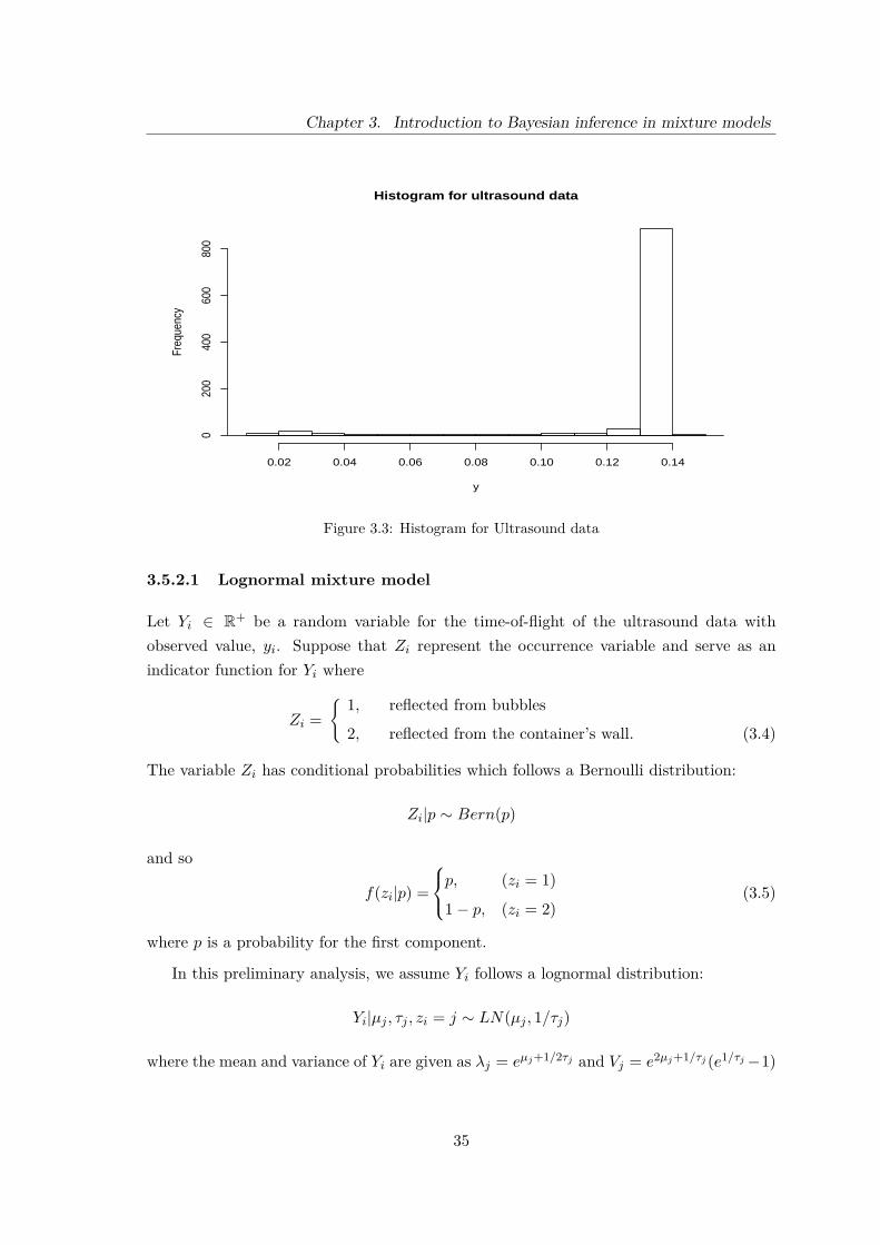
Chapter 3. Introduction to Bayesian inference in mixture models
Histogram for ultrasound data
y
Freq
uenc
y
0.02 0.04 0.06 0.08 0.10 0.12 0.14
020
040
060
080
0
Figure 3.3: Histogram for Ultrasound data
3.5.2.1 Lognormal mixture model
Let Yi ∈ R+ be a random variable for the time-of-flight of the ultrasound data withobserved value, yi. Suppose that Zi represent the occurrence variable and serve as anindicator function for Yi where
Zi ={ 1, reflected from bubbles
2, reflected from the container’s wall. (3.4)
The variable Zi has conditional probabilities which follows a Bernoulli distribution:
Zi|p ∼ Bern(p)
and so
f(zi|p) =
p, (zi = 1)
1− p, (zi = 2)(3.5)
where p is a probability for the first component.
In this preliminary analysis, we assume Yi follows a lognormal distribution:
Yi|µj , τj , zi = j ∼ LN(µj , 1/τj)
where the mean and variance of Yi are given as λj = eµj+1/2τj and Vj = e2µj+1/τj (e1/τj−1)
35
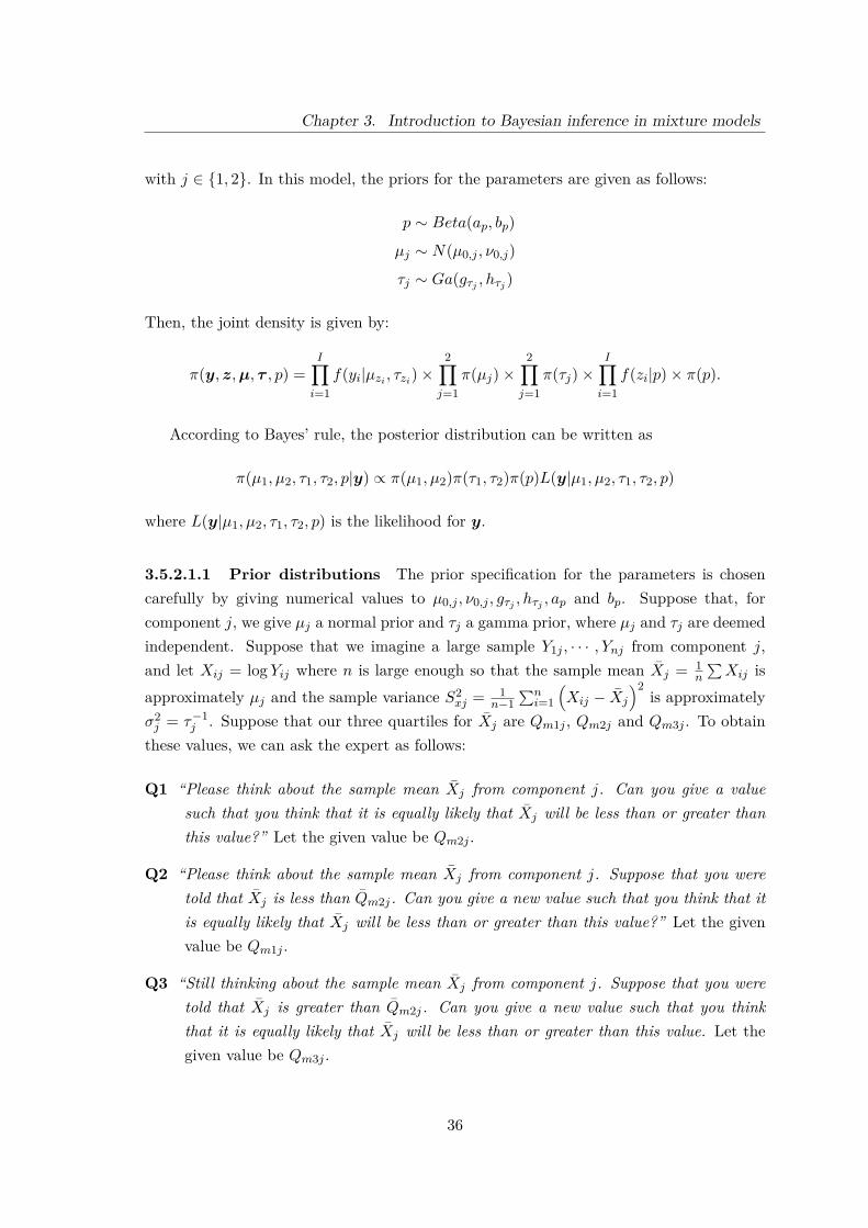
Chapter 3. Introduction to Bayesian inference in mixture models
with j ∈ {1, 2}. In this model, the priors for the parameters are given as follows:
p ∼ Beta(ap, bp)
µj ∼ N(µ0,j , ν0,j)
τj ∼ Ga(gτj , hτj )
Then, the joint density is given by:
π(y, z,µ, τ , p) =I∏i=1
f(yi|µzi , τzi)×2∏j=1
π(µj)×2∏j=1
π(τj)×I∏i=1
f(zi|p)× π(p).
According to Bayes’ rule, the posterior distribution can be written as
π(µ1, µ2, τ1, τ2, p|y) ∝ π(µ1, µ2)π(τ1, τ2)π(p)L(y|µ1, µ2, τ1, τ2, p)
where L(y|µ1, µ2, τ1, τ2, p) is the likelihood for y.
3.5.2.1.1 Prior distributions The prior specification for the parameters is chosencarefully by giving numerical values to µ0,j , ν0,j , gτj , hτj , ap and bp. Suppose that, forcomponent j, we give µj a normal prior and τj a gamma prior, where µj and τj are deemedindependent. Suppose that we imagine a large sample Y1j , · · · , Ynj from component j,and let Xij = log Yij where n is large enough so that the sample mean Xj = 1
n
∑Xij is
approximately µj and the sample variance S2xj = 1
n−1∑ni=1
(Xij − Xj
)2is approximately
σ2j = τ−1
j . Suppose that our three quartiles for Xj are Qm1j , Qm2j and Qm3j . To obtainthese values, we can ask the expert as follows:
Q1 “Please think about the sample mean Xj from component j. Can you give a valuesuch that you think that it is equally likely that Xj will be less than or greater thanthis value?” Let the given value be Qm2j .
Q2 “Please think about the sample mean Xj from component j. Suppose that you weretold that Xj is less than Qm2j. Can you give a new value such that you think that itis equally likely that Xj will be less than or greater than this value?” Let the givenvalue be Qm1j .
Q3 “Still thinking about the sample mean Xj from component j. Suppose that you weretold that Xj is greater than Qm2j. Can you give a new value such that you thinkthat it is equally likely that Xj will be less than or greater than this value. Let thegiven value be Qm3j .
36

Chapter 3. Introduction to Bayesian inference in mixture models
Then our prior mean for µj is µ0j = 12 (Qm1j +Qm3j) and our prior variance for µj is
v0j = [(Qm3j −Qm1j) /1.349]2.
Suppose that our three quartiles for S2xj are QS1j , QS2j and QS3j where we can gain
these point values using these questions:
Q4 “Please think about the sample variance S2xj from component j. Please give a value
such that S2xj is equally likely to be less than or greater than this value.” Let the given
value be QS2j .
Q5 “Still thinking about the sample variance S2xj from component j. Suppose that you
were told that S2xj is less than QS2j. Please give a new value such that it is equally
likely that S2xj is less than or greater than this value.”.Let the given value be QS1j .
Q6 “Still thinking about the sample variance S2xj from component j. Suppose that you
were told that S2xj is above than QS2j. Please give a new value such that it is equally
likely that S2xj is less than or greater than this value.” Let the given value be QS3j .
Then our three quartiles for τj are Q−1S3j , Q
−1S2j and Q−1
S1j . The parameter τj has aGa (gτj , hτj) distribution where gτj is chosen by iteratively solvingQ−1
S1j/Q−1S3j = R3 (gτj) /R1 (gτj),
where Rq(a) is quartile q for a Ga(a, 1) distribution, and hτj = R2 (gτj) /Q−1S2j .
Using this method, we have reasonable values which can be used for illustration asfollows:
Qm11 = −3.5 Qm31 = −2.5
Qm12 = −2.05 Qm32 = −1.95
QS11 = 0.5 QS21 = 0.8 QS31 = 1.2
QS12 = 0.0002 QS22 = 0.0004 QS32 = 0.0008
and henceµ01 = −3 v01 = 0.55
µ02 = −2 v02 = 0.005
gτ1 = 2.64 hτ1 = 1.85
gτ2 = 1.22 hτ2 = 0.0004.
Now, suppose that the probability of component 1 is given by p which follows a betadistribution. To elicit the prior for p, we can use these questions to ask the expert, basedon the hypothetical future sample method of Winkler (1967):
Q7 “Please give your assessment of the probability that a randomly chosen observationbelongs to component j.” Let the given value be m0 which is the prior mean for p.
37

Chapter 3. Introduction to Bayesian inference in mixture models
Q8 “Suppose that you were given a random sample of nf observations and that xf ofthese belonged to component j. With these additional data, what would now be yourassessment of the probability that a new observation would belong to component j?”Let the given value be mf . Note that actual numerical values are given for nf and xf .These are chosen in the light of the value given for m0, so that xf/nf is sufficientlydifferent from m0 and an initial judgement about the expert’s certainty about p.Larger values of nf are required if the expert has greater prior precision.
Then we have
apap + bp
= m0 and ap + xfap + bp + nf
= mf .
Solving these, we obtain
ap = m0
(nfmf − xfm0 −mf
)and bp = (1−m0)
(nfmf − xfm0 −mf
).
Using this method, we obtain illustrative values as follows:
m0 = 1/6 = 0.167, mf = 1/5 = 0.2
with nf = 12 and xf = 4. Hence
ap = 8, bp = 40.
For further discussion of relevant elicitation methods, see, for example, O’Hagan et al.(2006).
3.5.2.1.2 Posterior distributions The joint posterior distribution has been demon-strated in Section 3.5.2.1. To draw the posterior samples for the unknown parameters, anMCMC scheme was applied using the R JAGS package (Plummer, 2012). We also imposethe restriction µ1 < µ2 to avoid label switching. Following a burn-in of 5000 iterations, afurther 10000 iterations were taken to draw the posterior samples. The computing timethat was required to generate 10000 posterior draws was around 40 seconds by using Rsoftware on a 2.00GHz Samsung laptop 300V3A model with Intel Core i7-2630QM pro-cessor and 12 Gbytes of random-access memory. Based on the analysis, 10000 iterationsare sufficient to obtain the realisations from the posterior distribution since the chainsconverge after the initial burn-in period. The trace plots in Figure 3.4 indicate that themixing for all parameters is very satisfactory. Figure 3.5 shows the differences between
38
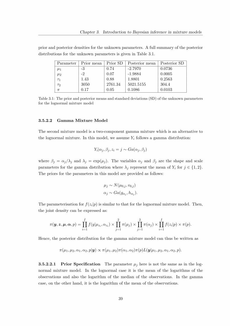
Chapter 3. Introduction to Bayesian inference in mixture models
prior and posterior densities for the unknown parameters. A full summary of the posteriordistributions for the unknown parameters is given in Table 3.1.
Parameter Prior mean Prior SD Posterior mean Posterior SDµ1 -3 0.74 -2.7970 0.0736µ2 -2 0.07 -1.9884 0.0005τ1 1.43 0.88 1.8801 0.2563τ2 3050 2761.34 5021.5155 304.4π 0.17 0.05 0.1086 0.0103
Table 3.1: The prior and posterior means and standard deviations (SD) of the unknown parametersfor the lognormal mixture model
3.5.2.2 Gamma Mixture Model
The second mixture model is a two-component gamma mixture which is an alternative tothe lognormal mixture. In this model, we assume Yi follows a gamma distribution:
Yi|αj , βj , zi = j ∼ Ga(αj , βj)
where βj = αj/λj and λj = exp(µj). The variables αj and βj are the shape and scaleparameters for the gamma distribution where λj represent the mean of Yi for j ∈ {1, 2}.The priors for the parameters in this model are provided as follows:
µj ∼ N(µ0,j , v0,j)
αj ∼ Ga(gαj , hαj ).
The parameterisation for f(zi|p) is similar to that for the lognormal mixture model. Then,the joint density can be expressed as:
π(y, z,µ,α, p) =I∏i=1
f(y|µzi , αzi)×2∏j=1
π(µj)×2∏j=1
π(αj)×I∏i=1
f(zi|p)× π(p).
Hence, the posterior distribution for the gamma mixture model can thus be written as
π(µ1, µ2, α1, α2, p|y) ∝ π(µ1, µ2)π(α1, α2)π(p)L(y|µ1, µ2, α1, α2, p).
3.5.2.2.1 Prior Specification The parameter µj here is not the same as in the log-normal mixture model. In the lognormal case it is the mean of the logarithms of theobservations and also the logarithm of the median of the observations. In the gammacase, on the other hand, it is the logarithm of the mean of the observations.
39

Chapter 3. Introduction to Bayesian inference in mixture models
µ1
Iteration
Val
ue
0 200 400 600 800 1000
−3.
0−
2.9
−2.
8−
2.7
−2.
6
µ2
IterationV
alue
0 200 400 600 800 1000
−1.
9900
−1.
9890
−1.
9880
−1.
9870
τ1
Iteration
Val
ue
0 200 400 600 800 1000
1.0
1.5
2.0
2.5
3.0
τ2
Iteration
Val
ue
0 200 400 600 800 1000
4500
5000
5500
6000
p
Iteration
Val
ue
0 200 400 600 800 1000
0.08
0.09
0.10
0.11
0.12
0.13
0.14
Figure 3.4: The trace plots for the first 1000 iterations of µ1, µ2, τ1, τ2 and p for the lognormalmixture model
40
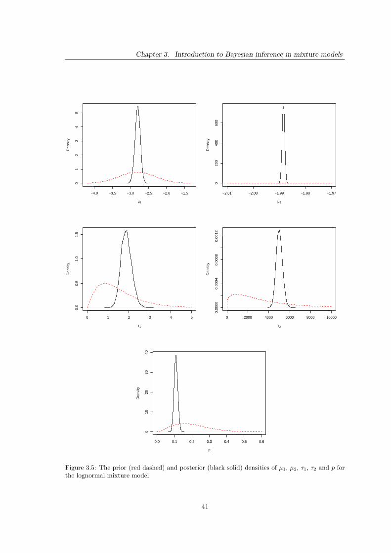
Chapter 3. Introduction to Bayesian inference in mixture models
−4.0 −3.5 −3.0 −2.5 −2.0 −1.5
01
23
45
µ1
Den
sity
−2.01 −2.00 −1.99 −1.98 −1.97
020
040
060
0
µ2
Den
sity
0 1 2 3 4 5
0.0
0.5
1.0
1.5
τ1
Den
sity
0 2000 4000 6000 8000 10000
0.00
000.
0004
0.00
080.
0012
τ2
Den
sity
0.0 0.1 0.2 0.3 0.4 0.5 0.6
010
2030
40
p
Den
sity
Figure 3.5: The prior (red dashed) and posterior (black solid) densities of µ1, µ2, τ1, τ2 and p forthe lognormal mixture model
41
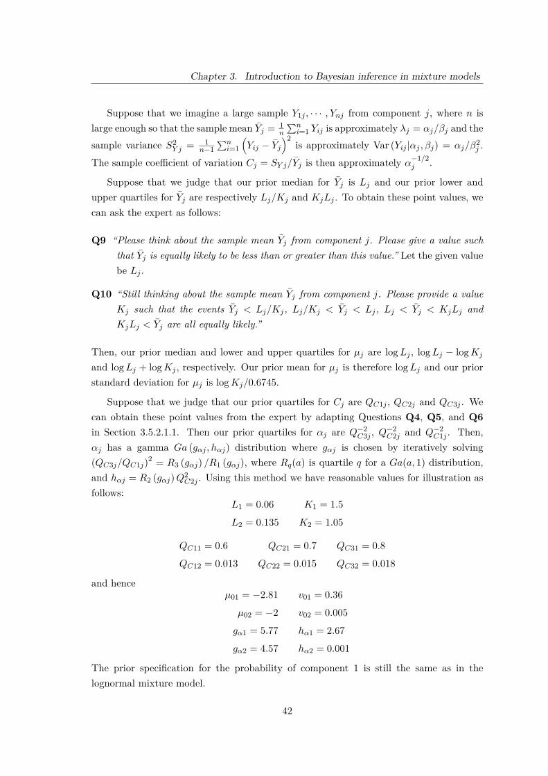
Chapter 3. Introduction to Bayesian inference in mixture models
Suppose that we imagine a large sample Y1j , · · · , Ynj from component j, where n islarge enough so that the sample mean Yj = 1
n
∑ni=1 Yij is approximately λj = αj/βj and the
sample variance S2Y j = 1
n−1∑ni=1
(Yij − Yj
)2is approximately Var (Yij |αj , βj) = αj/β
2j .
The sample coefficient of variation Cj = SY j/Yj is then approximately α−1/2j .
Suppose that we judge that our prior median for Yj is Lj and our prior lower andupper quartiles for Yj are respectively Lj/Kj and KjLj . To obtain these point values, wecan ask the expert as follows:
Q9 “Please think about the sample mean Yj from component j. Please give a value suchthat Yj is equally likely to be less than or greater than this value.” Let the given valuebe Lj .
Q10 “Still thinking about the sample mean Yj from component j. Please provide a valueKj such that the events Yj < Lj/Kj, Lj/Kj < Yj < Lj, Lj < Yj < KjLj andKjLj < Yj are all equally likely.”
Then, our prior median and lower and upper quartiles for µj are logLj , logLj − logKj
and logLj + logKj , respectively. Our prior mean for µj is therefore logLj and our priorstandard deviation for µj is logKj/0.6745.
Suppose that we judge that our prior quartiles for Cj are QC1j , QC2j and QC3j . Wecan obtain these point values from the expert by adapting Questions Q4, Q5, and Q6in Section 3.5.2.1.1. Then our prior quartiles for αj are Q−2
C3j , Q−2C2j and Q−2
C1j . Then,αj has a gamma Ga (gαj , hαj) distribution where gαj is chosen by iteratively solving(QC3j/QC1j)2 = R3 (gαj) /R1 (gαj), where Rq(a) is quartile q for a Ga(a, 1) distribution,and hαj = R2 (gαj)Q2
C2j . Using this method we have reasonable values for illustration asfollows:
L1 = 0.06 K1 = 1.5
L2 = 0.135 K2 = 1.05
QC11 = 0.6 QC21 = 0.7 QC31 = 0.8
QC12 = 0.013 QC22 = 0.015 QC32 = 0.018
and henceµ01 = −2.81 v01 = 0.36
µ02 = −2 v02 = 0.005
gα1 = 5.77 hα1 = 2.67
gα2 = 4.57 hα2 = 0.001
The prior specification for the probability of component 1 is still the same as in thelognormal mixture model.
42

Chapter 3. Introduction to Bayesian inference in mixture models
3.5.2.2.2 Posterior distribution The form of the joint posterior distribution wasgiven in Section 3.5.2.2. We used a similar approach as for the lognormal mixture modelby using an MCMC scheme to draw posterior samples for the unknown parameters. Here,the MCMC chain is run for 5000 iterations as burn-in and then a further 10000 iterationswere obtained as the posterior samples. Similar to the lognormal mixture model, thecomputing time that was used to obtain 10000 posterior draws is around 1.3 minutesusing the same software and machine. Based on the trace plots in Figure 3.6, the chainconverges very well and the mixing appears to be very satisfactory for all parameters. Theprior and posterior densities of the unknown parameters are shown in Figure 3.7. Thefull summary of the posterior distributions for the unknown parameters is given in Table3.2. In addition, Figure 3.8 shows the comparison of posterior density of the mean,
Parameter Prior mean Prior SD Posterior mean Posterior SDα1 2.16 0.9 2.4490 0.2951α2 4570 2137.76 5099.9498 302.7µ1 -2.81 0.6 -2.5733 0.0638µ2 -2 0.07 -1.9882 0.0005π 0.17 0.05 0.1102 0.0105
Table 3.2: The prior and posterior means with standard deviations (SD) of the unknown parametersfor the gamma mixture model
λj for component 1 and 2 for both models. From this figure, there are some differencesbetween the lognormal and gamma mixture models for component 1 but there are no largedifferences for component 2. These differences might be attributed to the different shapeof the distributions. In component 2, where α2 is large, there is little difference in shape.
43

Chapter 3. Introduction to Bayesian inference in mixture models
α1
Iteration
Valu
e
0 200 400 600 800 1000
2.0
2.5
3.0
3.5
α2
IterationVa
lue
0 200 400 600 800 1000
4500
5000
5500
6000
µ1
Iteration
Valu
e
0 200 400 600 800 1000
−2.8
−2.7
−2.6
−2.5
−2.4
µ2
Iteration
Valu
e
0 200 400 600 800 1000
−1.9
895
−1.9
885
−1.9
875
p
Iteration
Valu
e
0 200 400 600 800 1000
0.08
0.09
0.10
0.11
0.12
0.13
0.14
Figure 3.6: The trace plots for the first 1000 iterations of α1, α2, µ1, µ2 and p for the gammamixture model
44
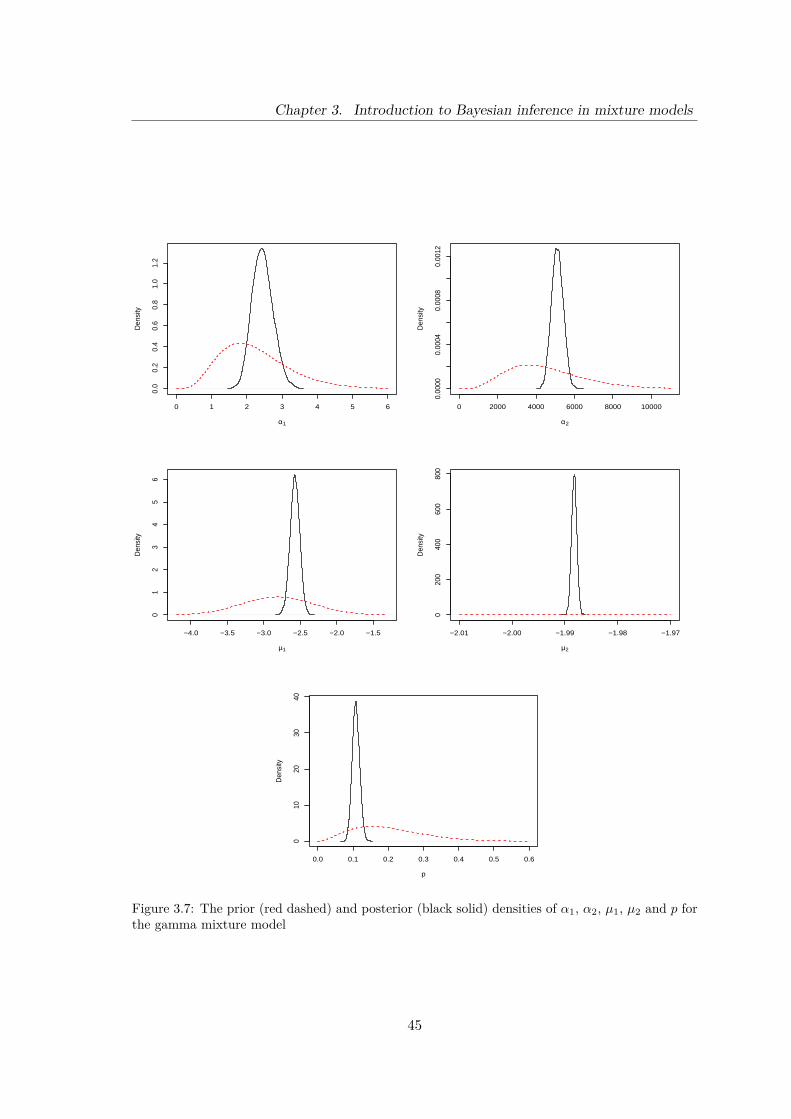
Chapter 3. Introduction to Bayesian inference in mixture models
0 1 2 3 4 5 6
0.0
0.2
0.4
0.6
0.8
1.0
1.2
α1
Den
sity
0 2000 4000 6000 8000 10000
0.00
000.
0004
0.00
080.
0012
α2D
ensi
ty
−4.0 −3.5 −3.0 −2.5 −2.0 −1.5
01
23
45
6
µ1
Den
sity
−2.01 −2.00 −1.99 −1.98 −1.97
020
040
060
080
0
µ2
Den
sity
0.0 0.1 0.2 0.3 0.4 0.5 0.6
010
2030
40
p
Den
sity
Figure 3.7: The prior (red dashed) and posterior (black solid) densities of α1, α2, µ1, µ2 and p forthe gamma mixture model
45
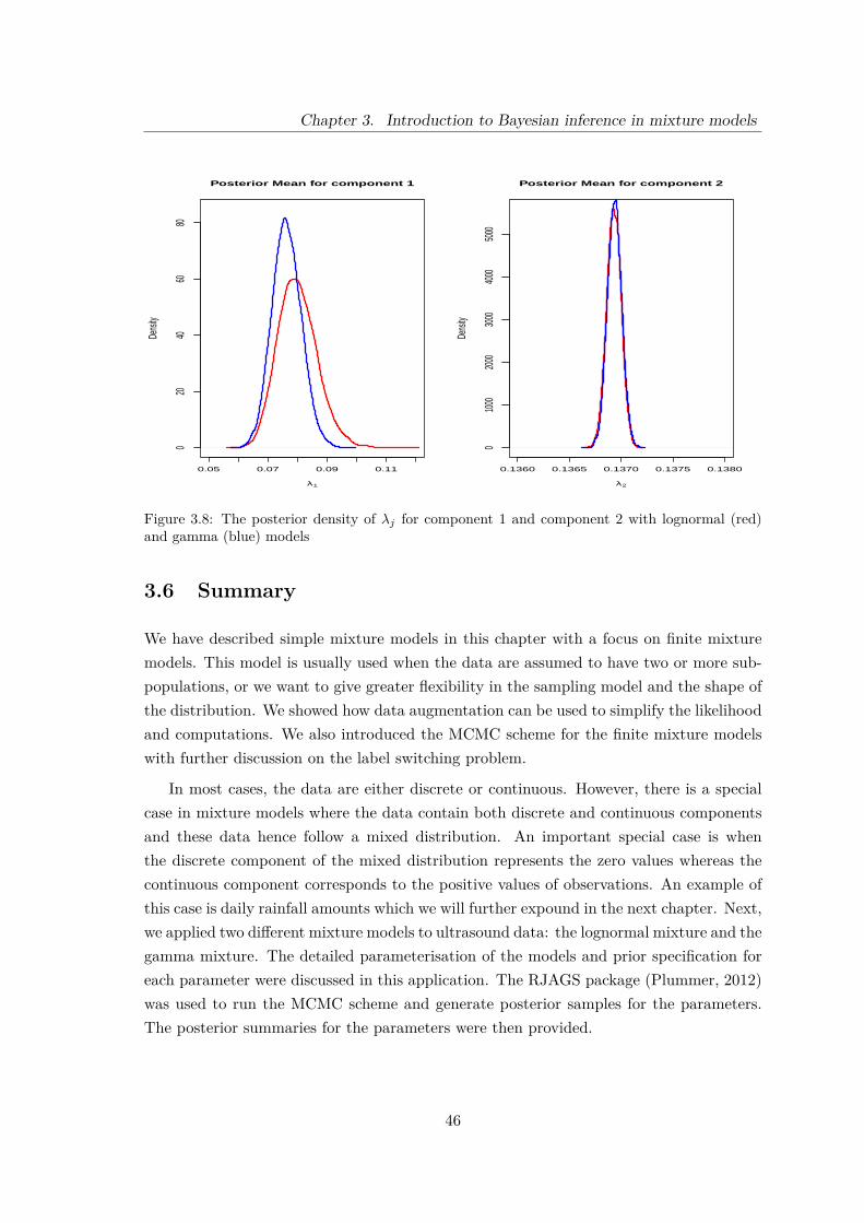
Chapter 3. Introduction to Bayesian inference in mixture models
0.05 0.07 0.09 0.11
020
4060
80Posterior Mean for component 1
λ1
Dens
ity
0.1360 0.1365 0.1370 0.1375 0.1380
010
0020
0030
0040
0050
00
Posterior Mean for component 2
λ2
Dens
ity
Figure 3.8: The posterior density of λj for component 1 and component 2 with lognormal (red)and gamma (blue) models
3.6 Summary
We have described simple mixture models in this chapter with a focus on finite mixturemodels. This model is usually used when the data are assumed to have two or more sub-populations, or we want to give greater flexibility in the sampling model and the shape ofthe distribution. We showed how data augmentation can be used to simplify the likelihoodand computations. We also introduced the MCMC scheme for the finite mixture modelswith further discussion on the label switching problem.
In most cases, the data are either discrete or continuous. However, there is a specialcase in mixture models where the data contain both discrete and continuous componentsand these data hence follow a mixed distribution. An important special case is whenthe discrete component of the mixed distribution represents the zero values whereas thecontinuous component corresponds to the positive values of observations. An example ofthis case is daily rainfall amounts which we will further expound in the next chapter. Next,we applied two different mixture models to ultrasound data: the lognormal mixture and thegamma mixture. The detailed parameterisation of the models and prior specification foreach parameter were discussed in this application. The RJAGS package (Plummer, 2012)was used to run the MCMC scheme and generate posterior samples for the parameters.The posterior summaries for the parameters were then provided.
46
Chapter 4
Modelling Univariate DailyRainfall Data
4.1 Introduction
The literature of time series modelling is immense and involves many approaches andparameterisations. In some circumstances, the time series data consist of positive and zerovalues. This type of data is quite challenging since it requires models for both discrete andcontinuous components. A distribution of this type is known as a mixed distribution. Thisfrequently materializes in many application areas such as meteorology, ecology, economicsand environmental sciences. A well-known example is the daily rainfall whose values areeither positive if rain occurs or zero if rain is absent.
This chapter introduces the idea of modelling daily rainfall data within the Bayesianframework. In this chapter, we only fit the daily rainfall data for one site with twodifferent applications before extending it to multiple locations in the next chapter. Section4.2 outlines the basic model for modelling mixed distributions. In this section, we willgive detailed descriptions on how to model the amount and occurrence processes. Thismethod will be subsequently applied to daily rainfall data in Italy in Section 4.3. Theprior beliefs will be incorporated with the likelihood of the data to obtain the posteriordistribution using MCMC. In addition, we also endeavour to determine and propose thebest probability density function (pdf) to represent the amount process. To accomplishthis, three pdfs will be considered to fit the daily rainfall data.
Next, in Section 4.4, we will extend the rainfall model developed in Section 4.3 by in-corporating the atmospheric circulation pattern, which is also known as the Lamb weathertype (LWT), into the British daily rainfall model. The LWT is included in the model byallowing the rainfall occurrence probabilities and the mean of the amount distribution to
47

Chapter 4. Modelling Univariate Daily Rainfall Data
be dependent upon the LWT. This will result in a more complex and challenging modelconstruction. Relating the occurrence probabilities and the amounts directly to the LWTis in contrast to the approach of Germain (2010) and Heaps et al. (2015) who introduceda latent “weather state” between the LWT and the observed rainfall. In addition Ger-main (2010) and Heaps et al. (2015) considered only winter rainfall and did not includeseasonal effects in the model. Seasonal effects will be introduced in Section 4.2.4. MCMCtechniques will be used to evaluate the posterior distribution for each model parameter.This will be discussed in detail in each section.
4.2 Modelling Daily Rainfall : The Basic Model
4.2.1 General structure
In this section, we shall describe the construction of a general daily rainfall model for asingle site. This work aims to provide the methodology required for modelling daily rainfallwithin the Bayesian framework before this can be extended to multiple sites. Modellingdaily rainfall data is a complex process since the distribution is a mixture of discrete andcontinuous components. Daily rainfall models commonly distinguish between the discretecomponent which represents rainfall occurrence and the continuous counterpart whichcorresponds to the rainfall amount when rain occurs. Hence, the daily rainfall can bemodelled separately in two parts: the occurrence process and the amount process. Theoccurrence process is a process that models the probability of rainfall occurrences whichmeans that the data has a zero value when rain is absent and a positive value when rainoccurs. On the other hand, the amount process is a process that models the amount ofrainfall which occurs during a rainy day. It is hence important to represent the rainfallamount with an appropriate distribution that only allows non-negative values.
Over the past few decades, most research using mixed distributions has advocated theuse of a two-stage approach. Stern & Coe (1984) demonstrated that the utilisation ofa two-stage approach in a daily rainfall model is relatively straightforward for hydrologyapplications. Tooze et al. (2002) also employed the same approach for the analysis ofmedical expenditure in the United States. Both examples have demonstrated that thetwo-stage approach is an appropriate way to model mixed distributions.
Generalized Linear Models (GLMs) have also been employed to model a daily rainfall.The GLMs are an effective class of probability models which can accommodate varioustypes of data such as climatological and meteorological data. The response variable for theGLM approach generally does not necessarily need to be Gaussian, as long as it comes fromone of the members of the exponential family. Therefore, GLMs can handle non-normal
48
Chapter 4. Modelling Univariate Daily Rainfall Data
responses using well defined characteristics for modelling the continuous and strictly pos-itive amount process and the discrete component of occurrence process. Basically, theresponse variable is linked to the linear predictor through a specific link function. Theearly works by Coe & Stern (1982) and Stern & Coe (1984) have shown that it is quitestraightforward to model daily rainfall using GLMs in a hydrology context. They used asimple linear regression with a Fourier series function as the covariate for both amountand occurrence processes. Grunwald & Jones (2000) utilised a similar approach to this inan Australian daily rainfall model by incorporating more complex covariates in the GLMmodel. Moreover, recent literature in rainfall modelling indicates that the covariates in theGLM may also include sophisticated weather variables such as temperature, wind speed,and atmospheric circulation pattern (Chandler & Wheater, 2002; Furrer & Katz, 2007).The GLM approach can also be extended to include spatio-temporal models. Chandler& Wheater (2002), Yang et al. (2005) and Fernandes et al. (2009) successfully proposeda GLM-based framework for spatiotemporal structure in daily rainfall models, an ideawhich we will use in the next chapter. However, the majority of this literature in rainfallmodelling does not use the Bayesian approach. Therefore, we want to contribute to thissmall literature and utilise the ideas from Coe & Stern (1982), Stern & Coe (1984) andGrunwald & Jones (2000) by using a Fourier series function as a covariate for both theamount and occurrence processes within the Bayesian framework. Particular attention isalso given to the relationship between these two processes. For the case of British dailyrainfall, we will extend the model by incorporating Lamb weather types (LWTs) directlyto the amount and occurrence processes.
Let Wt ∈ R+ be a random variable for the daily rainfall amount with an observedvalue, wt at a single site at time t (measured in days), where t = 1, . . . , T . Suppose thateach observation in the daily rainfall data is generated from a random process where thedistribution of Wt, given quantities pt and µt (where 0 ≤ pt ≤ 1), can be defined as follows:
Fw(wt|pt, µt) = Pr (Wt ≤ wt|pt, µt) =
0, (wt < 0)
1− pt, (wt = 0)
ptFA(wt|µt), (wt > 0)
where FA(wt|µt) is the distribution function of the amount distribution. Hence Pr(Wt =0) = 1 − pt. Given that Wt > 0, the conditional pdf of Wt is f(wt|µt). Let Rt representthe rainfall occurrence and serve as an indicator function for Wt. Then we have:
Rt ={ 0, Wt = 0
1, Wt > 0. (4.1)
49

Chapter 4. Modelling Univariate Daily Rainfall Data
Thus, the random variable Wt can be re-expressed as:
Wt = I(Wt > 0)Yt= RtYt (4.2)
where Yt = g(Zt) is a continuous random variable and g(.) is some monotonic functiondefining a suitable transformation (e.g. exponential) together with the transformed value,Zt. Here Wt is the actual rainfall amount whose value could be zero but it is alwaysobserved. According to Stern & Coe (1984) and Grunwald & Jones (2000), Yt can beregarded as the intensity process which can also be viewed as the potential rainfall amount.The value of Yt is always positive but not always observed.
In order to describe the serial structure of the daily rainfall, it is necessary to considera model that can accommodate the relationship between the amount and occurrence pro-cesses. Stern & Coe (1984) does not explicitly take into account any relationship betweenthe probability of rainfall and the rainfall amount. It is hence one of our primary objectivesto relate these two processes in our modelling strategies so that no important informationabout the rainfall amount and occurrence is lost. Our goal is further emphasized by Toozeet al. (2002) who stressed that it is critical to elucidate the relationship between the prob-ability and the level of nonzero observation so that the accuracy and adequacy of analysismight be improved. There are several approaches that we can employ to expound therelationship between the rainfall amount and occurrence. In the first approach, we can fitthe occurrence process and then use that information to analyse the amount process asfollows:
Pr(Rt = 1) = pt and f(wt|Rt = 1) (4.3)
where f(wt|Rt = 1) is the conditional pdf for the rainfall amount when rt = 1. Alterna-tively, we can evaluate the model for the potential rainfall amount first, and then, computethe rainfall probability as:
f(yt) and Pr(Rt = 1|Yt = yt) = h(yt) (4.4)
where h(y) is some function for the rainfall probability which incorporates the informationcontained in the amount process. A third possibility is that we can use a property of thedistribution, such as the mean, µ, as a covariate of the rainfall probability to link betweenthe amount and occurrence processes.
Heaps et al. (2015) demonstrated the first approach by introducing two normal vari-ables, {Z0, Z1} where
Wt = I(Z0,t > 0) exp(Z1,t) = Rt exp(Z1,t)
50

Chapter 4. Modelling Univariate Daily Rainfall Data
with Z0,t as the occurrence function and Z1,t as the amount function. In this case,f(wt|Rt = 1) is a lognormal density and the authors included the Z0,t as the covari-ate of Z1,t for the log-rainfall amount. On the other hand, Sofia (2007) utilised the thirdapproach by conditioning the occurrence process on the mean of the log potential rainfallamount, ϑt using logistic regression for monthly rainfall data. Thus, the probability ofrainfall is given by
Pr(Wt > 0|ϑt) = pt = exp(ζ0 + ζ1ϑt)1 + exp(ζ0 + ζ1ϑt)
.
In this case, Rt and Yt are conditionally independent given ϑt so f(wt|Rt = 1, ϑt) =f(yt|ϑt). For example, we can have Zt = log(Yt) and, given ϑt, Zt has a normal distributionwith mean ϑt and Yt has a lognormal distribution.
While Germain (2010) and Heaps et al. (2015) used the first approach, in this the-sis we propose to investigate the other two approaches as alternative models for dailyrainfall, within the Bayesian framework. In particular, we will use the third approach,which was used by Sofia (2007), for the Italian daily rainfall and the second approach forthe British daily rainfall. We will also investigate the daily rainfall data over the wholeyear in our model instead of just focusing on the daily rainfall data in the winter as inthe case of Germain (2010) and Heaps et al. (2015), or monthly data, as in the case ofSofia (2007). Figure 4.1 illustrates the example of a directed acyclic graph (DAG) for thegeneral structure of the univariate daily rainfall model. This model is the first proposalthat we will use for the univariate daily rainfall in the context of the Italian data. In thismodel, · · · , Yt−1, Yt, Yt+1, · · · are assumed to be independent and only depend on µt whichchanges over time. It means that Yt variables are independent given the model parametersand not just conditionally independent given Rt. The detail of this model will be discussedin Section 4.3.2 and we will also examine the assumption of conditional independence inthe amount process, through analysis of residuals in Section 4.3.3.5. There are other possi-bilities which we might consider, such as direct dependence between · · · , Yt−1, Yt, Yt+1, · · ·as well as · · · , Rt−1, Rt, Rt+1, · · · but with a different context of rainfall data.
RtRt−1 Rt+1
µtµt−1 µt+1WtWt−1 Wt+1
YtYt−1 Yt+1
Figure 4.1: A DAG showing the temporal dependence structure of the Italian daily rainfall model
51

Chapter 4. Modelling Univariate Daily Rainfall Data
4.2.2 Amount Process
The ideal distribution for the amount process has been a topic of interest in the pastfew decades, especially in modelling daily rainfall. It is thus vital to choose the rightdistribution to model the rainfall amount. Several studies have been conducted to identifythe best distribution for daily rainfall. However, there is no general consensus on whichprobability density function is the best to represent rainfall amount (Wilks, 1990, Kedem etal 1990, Cho et al 2004). The most commonly utilised distributions for the amount processare gamma (Katz, 1977; Stern & Coe, 1984; Grunwald & Jones, 2000), lognormal (Toozeet al., 2002; Heaps et al., 2015) and power transformed truncated normal distributions(Sanso & Guenni, 1999). Other distributions that have been employed for the modellingof daily rainfall data are Weibull (Tooze et al., 2002), exponential (Fernandes et al., 2009),and mixed exponential distributions (Wilks, 1999).
For the amount process, f(yt|µt, θ) is the pdf for the potential rainfall amount witha range between 0 and ∞. If Yt and Rt are conditionally independent given µt thenf(wt|Rt = 1, µt) is equivalent to f(yt|µt, θ) except for dry days, where Wt = 0. Thedistribution for Yt still remains identical whether the day is wet or dry. However, Yt isnot observed if Wt = 0. For example, Yt could have a lognormal distribution and then,if Yt = exp(Zt), Zt has a normal distribution. We can then propose to utilise the GLMapproach for fitting the mean of the amount distribution as:
g(µt) = ηt (4.5)
ηt = x′tη
where g(.) is the link function, ηt is the linear predictor, η is a vector of coefficients and xtis the covariate vector for observation t that may consist of temporal covariates, seasonaland trend components, and weather variables (e.g. the Lamb weather type). For thisprocess, Yt and Ys where s 6= t could be conditionally independent given µt, µs and theshape of the distribution could also change when one of the parameters varies over time t.For this reason, it is useful to illustrate and monitor these changes using zero-continuousplots (as in Figure 3.2) as the shape could shift from time to time. This will be explainedin more detail using the Italian daily rainfall example.
4.2.3 Occurrence Process
The proportion of wet and dry days can be described by modelling the occurrence pro-cess. Let R = {R1, R2, · · · , Rt} denote the sequence of daily rainfall occurrence witht = 1, 2, · · · , T . The conditional distribution of the occurrence process given pt is a
52

Chapter 4. Modelling Univariate Daily Rainfall Data
Bernoulli distribution:Rt ∼ Bern(pt).
In the literature on rainfall models, the vast majority of studies have utilised the first-orderMarkov chain to model the occurrence probability and this was performed by assumingthat the conditional probability of rain occurrence on a specific day only depends on theoccurrence of rainfall on the previous day (Gabriel & Neumann, 1962; Coe & Stern, 1982;Stern & Coe, 1984; Suhaila et al., 2011; Grunwald & Jones, 2000). For instance, Gabriel &Neumann (1962) successfully demonstrated that the sequence of daily rainfall occurrencein Tel Aviv, Israel could be modelled by using the first-order Markov chain. The Markovchain can also be extended to higher-order models. However, Jimoh & Webster (1996)found that a first-order Markov chain model is sufficient to predict the daily rainfalloccurrence. In our case, it is thus reasonable to use the first-order Markov chain for theoccurrence process.
Similar to the amount process, we may also use a GLM approach, considering that theBernoulli distribution is a part of the exponential family. Following the GLM framework,the probability of rainfall occurrence is governed by the link function. Practically, let
h(pt) = ζt (4.6)
ζt = x′tζ
where h(.) is the link function, ζt is the linear predictor, ζ is a vector of coefficients andxt is the covariate vector. Without loss of generality, this is the same covariate vector asfor the amount process. There are several link functions that can be used to relate theobserved variable to the linear predictor. Most research has emphasized the use of thelogit link function to transform pt from a (0, 1) scale to a (−∞,+∞) scale (Stern & Coe,1984; Grunwald & Jones, 2000; Lima & Lall, 2009). By using a logistic transformation,the relationship between the linear predictor, ζt, and transition probabilities of rainfalloccurrence, pt, can be expressed as
ζt = log(
pt1− pt
)= logit {pt} (4.7)
with an inverse transformation of
pt = exp(ζt)1 + exp
(ζt) . (4.8)
From this relationship, the value of ζt → ∞ if pt → 1 and if pt → 0 then ζt → −∞.Alternatively, we can employ other link functions such as the probit link function which
53

Chapter 4. Modelling Univariate Daily Rainfall Data
is denoted by:ζt = Φ−1 {pt} ,
where Φ−1 is the inverse of the standard normal distribution function, or the complemen-tary log-log link:
ζt = log [− log {1− pt}] .
Since Heaps et al. (2015) used the first approach for linking the occurence and amountprocesses and used a lognormal amount distribution, in effect they used a probit link.Other authors in the rainfall modelling literature, such as Gabriel & Neumann (1962),Coe & Stern (1982), Stern & Coe (1984), Grunwald & Jones (2000), Sofia (2007) andFernandes et al. (2009), have used a logit link. We have chosen to use a logit link incommon with these authors and to provide a contrast to Heaps et al. (2015). Althoughthe shapes of the two link functions are quite similar, the use of the logit link may providean advantage in terms of computational speed since we do not have to evaluate a normalcumulative distribution function or its inverse.
4.2.4 Seasonal Effect
One of the novelties that are proposed in this study is dealing with seasonal effects, es-pecially when the rainfall data is expected to have a cyclical pattern. In temperate andsubpolar regions such as the European countries, daily rainfall occurrence may be affectedby seasonal changes where the mean rainfall amount and the frequency of occurrence mightbe different, for example, during the winter and the summer periods. The changes of theannual rainfall cycle are important in agricultural planning especially for determining theoptimal time for planting crops and for estimating the crop yields. Hence, it is reasonableto incorporate seasonal effect to evaluate the nature of rainfall variability for countries inthe temperate region. In the Heaps et al. (2015) model, only winter rainfall data wereused and the model did not incorporate seasonal effects.
The most popular method that is extensively used in meteorological studies for mod-elling periodic time series is a truncated Fourier series. The earlier work by Jones &Brelsford (1967) and West & Harrison (1997) have highlighted that the periodic structurein time series can be modelled by sinusoidal representations. Furthermore, Stern & Coe(1984) have adopted the Fourier series to evaluate daily rainfall occurrence and amount foragriculture planning. Grunwald & Jones (2000) used the same approach to describe theseasonal pattern of the occurrence and amount processes for the Australian daily rainfalldata.
The Fourier series consists of sine and cosine terms of harmonic frequencies with a
54

Chapter 4. Modelling Univariate Daily Rainfall Data
period ω and this can be represented as:
F (t) =F∑f=1
[afcos (ωf t) + bf sin (ωf t)] (4.9)
where F denotes the number of sinusoids and af and bf represent the Fourier coefficientswith ωf = 2πf/L, the angular frequency where L is the period. For daily data that exhibitan annual cyclic pattern, L = 365.25. This Fourier series representation can be furthermodified by performing further substitutions for af and bf . Let ϕf be a phase of theFourier function, then af and bf are given by:
af = Afcos(ϕf )
bf = −Af sin(ϕf ).
Then, we can define the amplitude, A and the phase, ϕf as
Af =√a2f + b2f
and
ϕf = −arctan (bf/af ) .
Using this information, we can reparameterise the Fourier function in equation (4.9) inthe following form:
F (t) =∑Ff=1Afcos (ωf t+ ϕf ) . (4.10)
Now, this alternative Fourier series representation is easier for interpretation than theoriginal Fourier series form.
To fit a Fourier function in the model, we need to determine the optimal numberof harmonics to be used for this purpose. We can opt for any reasonable number ofFourier harmonics, up to a maximum of 182. However, previous studies have advocatedthat the first three harmonics are generally adequate to model seasonal effects on rainfall(Liu et al., 2011; Roldan & Woolhiser, 1982; Richardson, 1981). We will therefore usethis recommendation when incorporating the seasonal effects into our models. We mayemploy both Fourier series forms to model the amount and occurrence processes for thedaily rainfall model that will also allow for seasonal variability.
55

Chapter 4. Modelling Univariate Daily Rainfall Data
4.2.5 Prior and Posterior Distributions
To complete the model, we need to specify the prior distribution for the parameters.Let θ be the unknown parameter vector. If we assume prior independence between theparameters for the amount and occurrence processes, the joint prior distribution is hencegiven by:
π(θ) = π(θamt)× π(θocc)
where π(θamt) and π(θocc) are the prior distributions for the amount and occurrence pro-cesses. Practically, prior selections for the unknown parameters should be based on ourprior beliefs, the information gained from the expert or from the previous studies. Forinstance, normal prior distributions are often assigned to the regression coefficients η andζ since η and ζ can take any value within the range of −∞ to ∞. Apart from the re-quirement that prior specifications should reflect reasonable prior beliefs, inappropriate orcareless specifications might also adversely affect, for example, the convergence of MCMCalgorithms.
Based on Bayes theorem, the posterior distribution of θ is proportional to likelihood× prior. Thus, the posterior distribution of θ can be written as:
π(θ|w, r) ∝ f(w|θ)× f(r|w,θ)× π(θ). (4.11)
To obtain samples from π(θ|w, r), we can use an MCMC scheme. The full conditionaldistribution (FCD) for each unknown parameter can be easily derived from Equation(4.11). If the FCD is in a standard form, we can draw samples directly from it. If it doesnot correspond to any standard density form, we need to use the Metropolis-Hastings(MH) algorithm to obtain samples. Thus, we use a Metropolis-within-Gibbs algorithm.
4.2.5.1 Priors in truncated Fourier representation of seasonality
In this section, we will describe prior distributions for Fourier series coefficients. Theprior distribution for Fourier parameters in Equation (4.9) is difficult to interpret. How-ever, we can think more directly about the prior distribution in terms of the phase andamplitude as in Equation (4.10). Suppose that we have (af , bf )′ ∼ N2(mf , Vf ) wheremf = (mf,a,mf,b)
′ and
Vf =(
v2f,a ρfvf,avf,b
ρfvf,avf,a v2f,b
).
56

Chapter 4. Modelling Univariate Daily Rainfall Data
We can derive the prior distribution for Af and ϕf using the fact that Af =√a2f + b2f
and ϕf = − arctan (bf/af ) ∈ [−π, π). The Jacobian of the transformation is given by
(∂(af , bf )∂(Af , ϕf )
)=
∂af∂Af
∂bf∂Af
∂af∂ϕf
∂bf∂ϕf
=
cos(ϕf ) − sin(ϕf )
−Af sin(ϕf ) −Af cos(ϕf )
and hence ∣∣∣∣∣det
(∂(af , bf )∂(Af , ϕf )
)∣∣∣∣∣ =∣∣∣−Af cos2(ϕf )−Af sin2(ϕf )
∣∣∣ = |−Af | = Af .
The density for (Af , ϕf )′ is therefore
f(Af , ϕf ) =f(af , bf )∣∣∣∣∣det
(∂(af , bf )∂(Af , ϕf )
)∣∣∣∣∣Af
2πvf,avf,a√
1− ρ2f
exp{−Q(Af , ϕf )
2(1− ρ2f )
}
where
Q(Af , ϕf ) =(Af sin(ϕf )−mf,a)2
v2f,a
− 2ρf (Af sin(ϕf )−mf,a) (Af cos(ϕf )−mf,b)vf,avf,b
+ (Af cos(ϕf )−mf,b)2
v2f,b
for Af ≥ 0 and ϕ ∈ [−π, π). Assuming mf,a = mf,b = 0 and vf,a = vf,b = vf , the densitysimplifies to
f(Af , ϕf ) = Af
2πv2f
√1− ρ2
f
exp{−
A2f
2v2f (1− ρ2
f ){1− ρf sin(2ϕf )} .
}(4.12)
This density can be further simplified by assuming ρf = 0 which gives
f(Af , ϕf ) = Afv2f
exp{−A2f
2v2f
.
}× 1
2π .
In this case, it is clear that Af and ϕf are independent and
Af ∼ Ray(vf ) and ϕ ∼ U(−π, π)
where Ray(vf ) denotes the Rayleigh distribution with scale parameter, vf .
57

Chapter 4. Modelling Univariate Daily Rainfall Data
Provided that we wish to give the phase a uniform prior, this provides a convenientway to convert a prior for the amplitude into a bivariate normal prior for the Fouriercoefficients. This may be appropriate for the higher frequencies. In the case of the funda-mental frequency, with period one year, and perhaps the second frequency, we may wellhave prior information about the annual pattern of rainfall which we can use. In this casewe can give the phase a more informative prior, for example a von Mises distribution. Inthis case the distribution of the Fourier coefficients will not be bivariate normal. The vonMises distribution is not a standard distribution in JAGS. While, of course, we need notuse JAGS and could use a specially-written sampler, in principle we can also overcome thedifficulty by using, for example, the “ones trick” (Lunn et al., 2012, Chapter 9) in JAGS.
However a more direct approach is as follows. Suppose that we wish to use F harmon-ics. We can choose 2F time-points during the year and elicit beliefs about the value ofthe seasonal term at these times. The times might include, for example the times whichare expected to give the maximum and minimum of the seasonal effect. Let the times bet1, . . . , t2F . Then, using elicitation questions in which other model quantities are fixed asappropriate, we can first elicit marginal means and variances for F1, . . . , F2F where Fj isthe value of the seasonal effect at time tj . So
Fj =F∑f=1
[af cos(ωf tj) + bf sin(ωf tj)].
We choose a multivariate normal prior distribution for F = (F1, . . . , F2F )′ and assumethat this will adequately represent prior beliefs. It remains to specify covariances betweenthe elements of F. In the style of Farrow (2003) we write
Fj − E(Fj) = kj{U0 + U1 cos(ωtj) + U2 sin(ωtj) + Ej}
where ω = 2π/365.25, U0, U1, U2 and E1, . . . , E2F are all independent, zero-mean randomvariables and Var(U0) = V0, Var(U1) = Var(U1) = V1 and Var(Ej) = VE . We constrainV0 +V1 +VE = 1. Hence the marginal variance is Var(Fj) = k2
j . The covariances are givenby
Covar(Fj , Fh) = V0 + V1(cosωtj cosωth + sinωtj sinωth) = V0 + V1 cos(ω[tj − th]).
By choosing values for V0, V1 and VE , we determine a covariance matrix VF for F.
Now we can writeF = Tc
where c = (a1, . . . , aF , b1, . . . , bF )′ and T is a 2F×2F matrix where column f is (cosωf t1, . . . , cosωf tF )′
58

Chapter 4. Modelling Univariate Daily Rainfall Data
and column f + F is (sinωf t1, . . . , sinωf tF )′. Then c = T−1F and the covariance matrixof c is T−1VF (T−1)′. Thus we obtain a multivariate normal prior distribution for the setof Fourier coefficients.
4.2.6 Diagnostic checking for mixed-distribution time series
One class of diagnostic checks for the non-standard time series models has been proposedby Smith (1985) to assess whether the fitted model is well calibrated. The author intro-duced two types of residuals for the diagnostic checking which are the “forecast distributiontransformed residuals” (FDTR) and the normal-transformed version called “normal fore-cast transformed residuals” (NFTR). An important feature of the FDTR is that, whenthe distribution of the observations is continuous and if the observations are drawn fromthe forecast distribution, the FDTR are distributed uniformly U(0, 1). If the observationswere generated according to our model and we knew the true values of the parameters andused these values to calculate the forecast distribution, the FDTR would then be indepen-dent. Since we do not know the values of the parameters and our forecast distribution isa posterior predictive distribution, the FDTR will only be approximately independent.
In the case of rainfall, the distribution of the observations is not continuous since it is amixture of zeros (discrete) and positive values (continuous). Therefore, some modificationsare required to make the Smith (1985) method work. Smith (1985) already discusses ingreat detail how to deal with the case where the observation distribution is discrete. Inour case, we need to do something similar and we therefore choose that, instead of workingin terms of the observations on the random variable W , which has a mixed distribution,we define another random variable U , which has a continuous distribution, and work interms of this. Of course U and W are closely related and, in fact, given the value of U ,we can find the value of W . Thus, we propose to define U as follows:
• If W > 0 then U = W .
• If W = 0 then U is drawn from a uniform U(−1, 0) distribution. In fact, we could useany continuous distribution on (−∞, 0] for this purpose but this uniform distributionis sufficiently convenient.
Hence, we simulate the values of U for the days with zero rainfall and use these as data. Wethen use the forecast distributions of U , rather than W , and compare the observed valuesof U with these distributions. The FDTR should then have a uniform U(0, 1) distributionas required. NFTR can be obtained by using
VU = Φ−1(U)
59

Chapter 4. Modelling Univariate Daily Rainfall Data
where Φ is the standard normal distribution function. If the fitted model is “good”, thenthe residuals U and VU should be approximately independent and follow the uniformU(0, 1) or standard normal, N(0, 1) distributions. If the residuals are unsatisfactory, thenwe need to revise our model to improve the forecasting system by using the deviations in{U} and {V } from their expected forms (Smith, 1985).
4.3 Daily Rainfall Model for Urbino, Italy
4.3.1 Data
Figure 4.2: Location of daily rainfall in the city of Urbino, Italy
To apply the developed model, we utilized daily rainfall data from the Urbino raingauge station in Italy. Figure 4.2 shows the location of Urbino which is in the region ofMarche, the central area of Italy. We used daily rainfall data recorded from 1981 until2007 (27 years), a total of 9861 observations. These data have more zeros than positivevalues as indicated in Figure 4.3.
From Figure 4.3, we can see that the occurrence of rainfall is quite low, with incon-sistent rainfall patterns for each year. On average, the wettest days are usually betweenaround November and January, whilst the driest days took place in July and August. Thehighest recorded rainfall amount was on the 24th of November 1991 with a precipitation of113.8 mm. Fitting this type of rainfall data is considered very challenging since we havemore zeros than positive values. Hence, this warrants a more flexible modelling approach.This will be discussed in more detail in the next section.
60
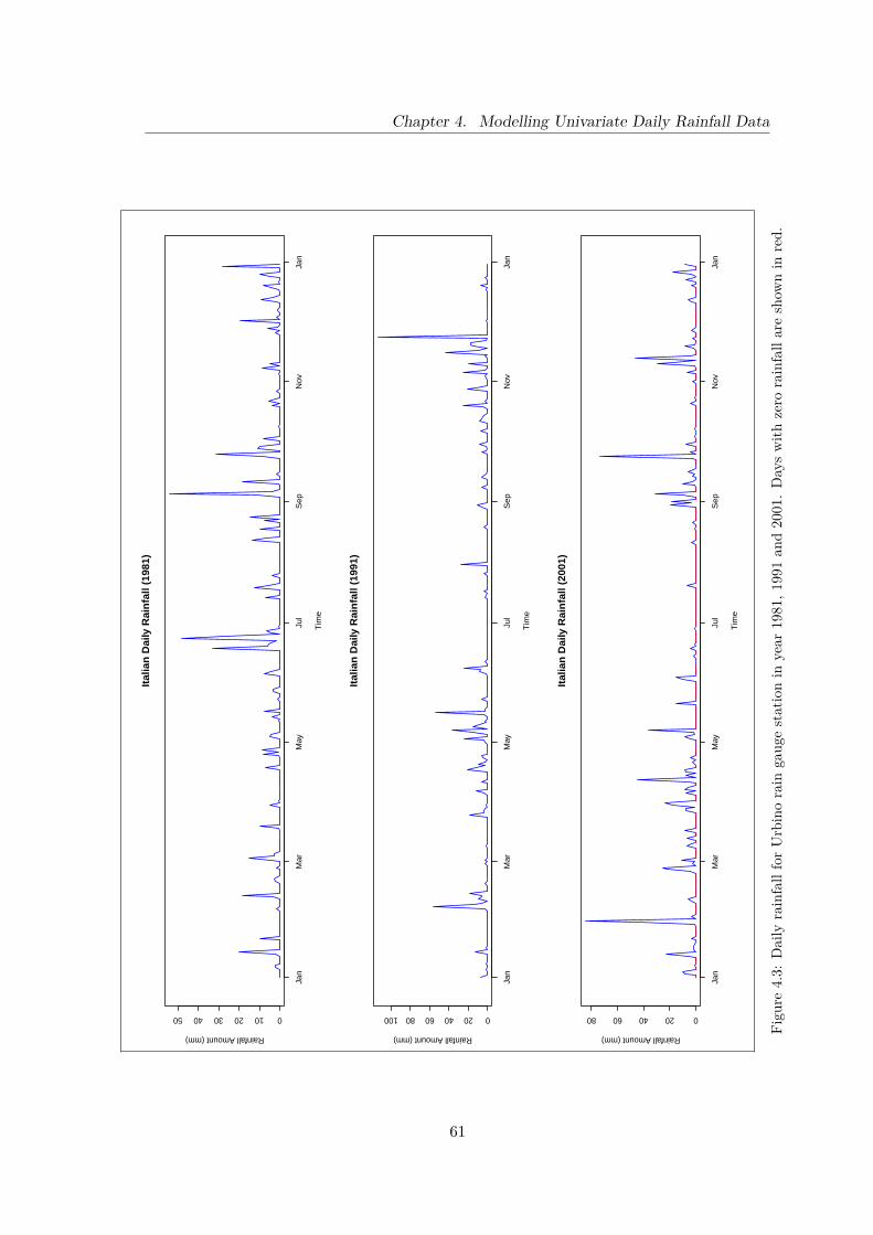
Chapter 4. Modelling Univariate Daily Rainfall Data
Jan
Mar
May
Jul
Sep
Nov
Jan
01020304050
Italia
n D
aily
Rai
nfal
l (19
81)
Tim
e
Rainfall Amount (mm)
Jan
Mar
May
Jul
Sep
Nov
Jan
020406080100
Italia
n D
aily
Rai
nfal
l (19
91)
Tim
e
Rainfall Amount (mm)
Jan
Mar
May
Jul
Sep
Nov
Jan
020406080
Italia
n D
aily
Rai
nfal
l (20
01)
Tim
e
Rainfall Amount (mm) Figu
re4.
3:D
aily
rain
fall
for
Urb
ino
rain
gaug
est
atio
nin
year
1981
,199
1an
d20
01.
Day
sw
ithze
rora
infa
llar
esh
own
inre
d.
61

Chapter 4. Modelling Univariate Daily Rainfall Data
4.3.2 The Model
4.3.2.1 Amount Process
In order to model the amount process, we utilised the ideas from Fernandes et al. (2009)and Suhaila et al. (2011) by which we chose several distributions so that we can assessand determine the best distribution for the amount process. To accomplish this, we willcompare the lognormal and gamma distributions since both distributions have 0 to ∞support, a desirable property for modelling the amount process. Cho et al. (2004) hadpreviously compared the lognormal and gamma distributions for rainfall data and theyestablished that the lognormal distribution is more appropriate for dry regions, whilst a wetregion is better modelled using a gamma distribution. However, we will use two differentparameterisations for the gamma distribution. For the first parameterisation, we shall usea gamma distribution with fixed shape parameter (α) and variable scale parameter, (β),denoted as “G1” distribution, and in the second parameterisation, a gamma distributionwith a variable shape parameter (α) and fixed scale parameter, (β), denoted as “G2”distribution, will be used. The full details of these distributions are given below:
• Lognormal distribution:The observed rainfall amount can be defined as
Wt = RtYt
where Yt is assumed to follow a lognormal distribution. If Zt = log(Yt), then Zt
follows a normal distribution with the probability density function given by:
f(zt|ϑt, τ) =√τ
2π exp{−τ2 (zt − ϑt)2
}(4.13)
where E(Zt) = ϑt and Var(Zt) = 1/τ . The mean and variance of Yt are given asµt = eϑt+1/2τ and Vyy = e2ϑt+1/τ (e1/τ − 1).
If Zt and Zs, s 6= t, are conditionally independent given ϑt, ϑs and τ , the likelihoodfunction for ϑt and τ is represented by:
L(ϑt, τ |zt) =T∏t=1
√τ
2π exp{−τ2 [zt − ϑt]2
}. (4.14)
This transformation allows us to evaluate the parameter in a much simpler andstraightforward way since a Gaussian distribution can be used. Sofia (2007) employedthe lognormal distribution to evaluate the monthly rainfall in the Mediterranean re-gion. Heaps et al. (2015) also used the lognormal distribution in non-homogeneous
62

Chapter 4. Modelling Univariate Daily Rainfall Data
hidden Markov models (NHMMs) for describing the rainfall amount during winter.Figure 4.4 shows different plots of probability density functions for the lognormal
0 1 2 3 4 5 6
0.0
0.5
1.0
1.5
Probability density for lognormal distribution
y
Dens
ity
ϑ= 1 , τ= 1ϑ= 0.5 , τ= 1ϑ= 0 , τ= 1ϑ= − 0.5 , τ= 1ϑ= − 1 , τ= 1
Figure 4.4: The forms of probability density function for lognormal distribution with different ϑ
distribution, each having different mean, ϑ and constant precision, τ , for the loga-rithm of rainfall amount. As we can clearly observe, the shape of the distributionis skewed to the right and its mode decreases as ϑ decreases. The density is alwayszero at y = 0.
• Gamma distribution:Another distribution that is widely used for rainfall amount representation is thegamma distribution. The gamma distribution is a popular choice for rainfall databecause it produces a good fit and its shape is approximately identical to the his-togram of rainfall data (Ben-Gai et al., 1998). The observed rainfall is hence givenby:
Wt = RtYt
where Yt follows a gamma distribution. The G1 distribution parameterisation isrepresented by:
f(yt|α, βt) = βαt yα−1t e−βtyt
Γ (α) (4.15)
with constant shape parameter, α > 0 and variable scale parameter, βt = α/µt. Themean of this distribution is E(Yt) = µt and the variance is Var(Yt) = µ2
t /α. If the
63

Chapter 4. Modelling Univariate Daily Rainfall Data
observations are conditionally independent over time, the likelihood function basedon the G1 distribution for α and µt is given by:
L(α, µt|yt) =T∏t=1
(α/µt)α yα−1t e−(α/µt)yt
Γ (α) . (4.16)
In Figure 4.5, the probability density function plots for gamma distributions with
0 1 2 3 4 5 6
0.0
0.5
1.0
1.5
Probability density for gamma distribution
y
Dens
ity
α=2 , β=4α=2 , β=3α=2 , β=2α=2 , β=1α=2 , β=0.5
Figure 4.5: The forms of probability density function for gamma distribution with different β
variable β and constant α = 2 are shown.
For the G2 distribution, the probability density function is specified as
f(yt|β, αt) = βαtyαt−1t e−βyt
Γ (αt)(4.17)
where αt = µtβ represents the variable shape parameter and β > 0 is the fixedscale parameter. The mean for this distribution is analogous to the mean of the G1distribution but the variance is dissimilar. Since we have fixed β, the variance for thisdistribution is Var(Yt) = µt/β. If the observations are assumed to be conditionallyindependent with time, then the likelihood function for β and µt is:
L(β, µt|yt) =T∏t=1
βµtβyµtβ−1t e−βyt
Γ (µtβ) . (4.18)
64
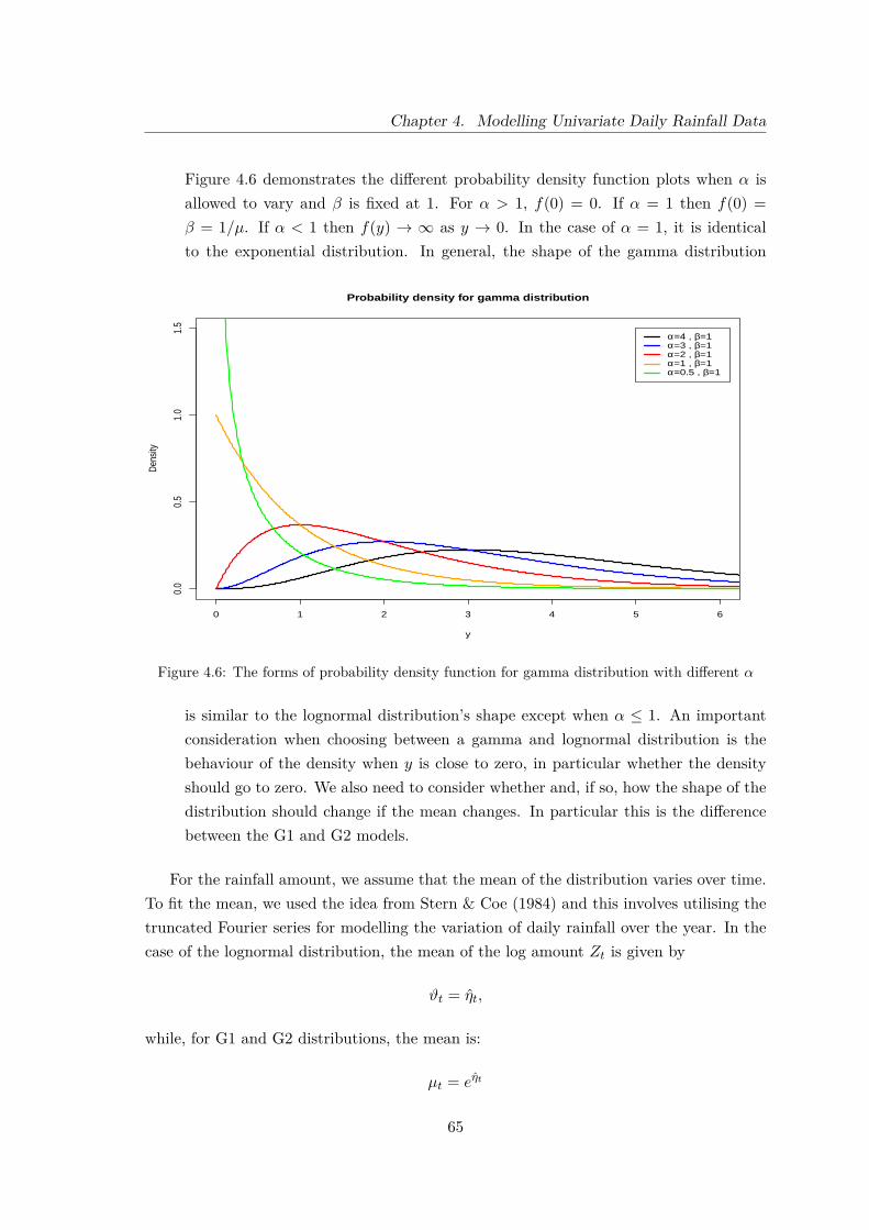
Chapter 4. Modelling Univariate Daily Rainfall Data
Figure 4.6 demonstrates the different probability density function plots when α isallowed to vary and β is fixed at 1. For α > 1, f(0) = 0. If α = 1 then f(0) =β = 1/µ. If α < 1 then f(y) → ∞ as y → 0. In the case of α = 1, it is identicalto the exponential distribution. In general, the shape of the gamma distribution
0 1 2 3 4 5 6
0.0
0.5
1.0
1.5
Probability density for gamma distribution
y
Dens
ity
α=4 , β=1α=3 , β=1α=2 , β=1α=1 , β=1α=0.5 , β=1
Figure 4.6: The forms of probability density function for gamma distribution with different α
is similar to the lognormal distribution’s shape except when α ≤ 1. An importantconsideration when choosing between a gamma and lognormal distribution is thebehaviour of the density when y is close to zero, in particular whether the densityshould go to zero. We also need to consider whether and, if so, how the shape of thedistribution should change if the mean changes. In particular this is the differencebetween the G1 and G2 models.
For the rainfall amount, we assume that the mean of the distribution varies over time.To fit the mean, we used the idea from Stern & Coe (1984) and this involves utilising thetruncated Fourier series for modelling the variation of daily rainfall over the year. In thecase of the lognormal distribution, the mean of the log amount Zt is given by
ϑt = ηt,
while, for G1 and G2 distributions, the mean is:
µt = eηt
65

Chapter 4. Modelling Univariate Daily Rainfall Data
where
ηt = η0 +F∑f=1
[afcos
( 2πft365.25
)+ bf sin
( 2πft365.25
)]. (4.19)
The parameter η0 is the common level for the amount of rainfall. We will use threeharmonics of the Fourier series as indicated in Section 4.2.4 to represent the seasonaleffect of the rainfall amount over the year.
4.3.2.2 Occurrence Process
In the Italian daily rainfall application, we use a first-order Markov chain to model theprobability of rainfall. The transition probabilities of the first-order Markov chain modelare given by:
pij(t) = Pr{rt = j|rt−1 = i}; i, j ∈ {0, 1},
with the transition matrix:
Pt =( rt = 0 rt = 1
rt−1 = 0 p00(t) p01(t)rt−1 = 1 p10(t) p11(t)
).
To represent the rainfall probability, we use a logistic link function to connect the predic-tors with the rainfall probability pi1(t):
logit [pi1(t)] = ζi,t; i = 0, 1.
If the distribution of Yt is a lognormal distribution, then the parameterisation for ζi,t isgiven by
ζi,t = ζ0 +F∑f=1
[cfcos
( 2πf365.25
)+ df sin
( 2πf365.25
)]+ ζ1ϑt + ζ2
(i− 1
2
). (4.20)
If Yt follows a gamma distribution, then we have
ζi,t = ζ0 +F∑f=1
[cfcos
( 2πf365.25
)+ df sin
( 2πf365.25
)]+ ζ1 log(µt) + ζ2
(i− 1
2
). (4.21)
The parameter ζ0 is a common intercept for logit [pi1(t)] and the term i is an indicatorfunction with a value of i = 1 if rain occurs on the previous day and i = 0 otherwise. Wealso included ϑt and log(µt) in Equations (4.20) and (4.21) to create a link between the
66

Chapter 4. Modelling Univariate Daily Rainfall Data
amount and occurrence processes so that the accuracy of the rainfall probability can beimproved. For instance, the rainfall probability increases if µt increases. We also employeda Fourier series with three harmonics for rainfall occurrence to allow for the seasonal effectover the year.
The conditional probabilities can be summarised as follows:
p11(t) =exp
(ζ1,t)
1 + exp(ζ1,t) ; p10(t) = 1− p11(t),
p01(t) =exp
(ζ0,t)
1 + exp(ζ0,t) ; p00(t) = 1− p01(t).
The unconditional probability can be represented by:
pt =p11(t)pt−1 + p01(t) (1− pt−1)
=p01(t) + [p11(t)− p01(t)] pt−1
pt + [p01(t)− p11(t)] pt−1 =p01(t).
We can write this asAP = p
and henceP = A−1p (4.22)
with P = (p1, · · · , p365)′, p = (p01(1), · · · , p01(365))′ and
A =
1 0 0 · · · 0 a1
a2 1 0 · · · 0 00 a3 1 · · · 0 0...
...... . . . ...
...0 0 0 · · · 1 00 0 0 · · · a365 1
where at = p01(t)− p11(t).
However, the parameterisation in Equations (4.20) and (4.21) may lead to poor mixingwhen we run the MCMC algorithm. To overcome this problem, we centered the predictorvariables as follows:
67
Chapter 4. Modelling Univariate Daily Rainfall Data
• lognormal distribution
ζi,t = ζ0 +F∑f=1
[cfcos
( 2πf365.25
)+ df sin
( 2πf365.25
)]+ ζ1 (ϑt − ζ0) + ζ2
(i− 1
2
).
(4.23)
• gamma distribution
ζi,t = ζ0 +F∑f=1
[cfcos
( 2πf365.25
)+ df sin
( 2πf365.25
)]+ ζ1 (log(µt)− ζ0) + ζ2
(i− 1
2
).
(4.24)
4.3.2.3 Prior specifications
This section provides the detailed descriptions on the construction of the prior distributionsfor the unknown parameters in our model. The prior density of the unknown parametersis represented by π(θ). Priors will be constructed based on the information acquired fromprevious studies and personal beliefs.
Suppose that the precision parameter, τ , in the lognormal distribution follows a gammadistribution:
τ ∼ Ga(gτ , hτ )
for fixed hyperparameters gτ and hτ since the values are strictly positive on the real line.This is a sensible choice because the gamma distribution is semi-conjugate to the likelihoodfunction of the lognormal form. For parameters α in the G1 distribution and β in theG2 distribution, we also assign gamma priors since their values are stricly positive. Thepriors are therefore:
α ∼ Ga(gα, hα); β ∼ Ga(gβ, hβ)
with fixed hyperparameters gα, hα, gβ and hβ.
In our model, we use a GLM approach to relate the linear predictor to the responsevariable using a link function for both the amount and occurrence processes. The set oflinear coefficients for the amount process is represented by η = (η0, a1, a2, a3, b1, b2, b3) andζ = (ζ0, ζ1, ζ2, c1, c2, c3, d1, d2, d3) is the parameter vector for the occurrence process. Sincethe linear predictor can take any values from −∞ to ∞, a normal prior for each unknownparameter in the linear predictors is appropriate. If we assume prior independence betweenthe parameters, then the priors for all parameters are given below:
68

Chapter 4. Modelling Univariate Daily Rainfall Data
• Amount process
η0 ∼ N(mA0, vA0) a1 ∼ N(ma1 , va1)
a2 ∼ N(ma2 , va2) a3 ∼ N(ma3 , va3)
b1 ∼ N(mb1 , vb1) bf ∼ N(mb2 , vb2)
b3 ∼ N(mb3 , vb3)
• Occurrence process
ζ0 ∼ N(mC0, vC0) ζ1 ∼ N(mC1, vC1)
ζ2 ∼ N(mC2, vC2) c1 ∼ N(mc1 , vc1)
c2 ∼ N(mc2 , vc2) c3 ∼ N(mc3 , vc3)
d1 ∼ N(md1 , vd1) d2 ∼ N(md2 , vd2)
d3 ∼ N(md3 , vd3).
We can relax the prior independence assumption by assigning a multivariate normal priorfor η and ζ :
η ∼ N7(η, P−1η )
ζ ∼ N9(ζ, P−1ζ )
where η and ζ represent the mean vectors with precisions Pη and Pζ .
4.3.2.4 Posterior distributions
The joint density of (θ,y, r) is given by:
π(θ,y, r) = π(θ)× f(y|θ)× f(r|θ)
= π(θamt)× π(θocc)×T∏t=1
f(yt|θamt)× f(r1 | θocc,θamt)T∏t=2
f(rt | rt−1,θocc,θamt).
Note that yt is only observed when rt = 1. To obtain the posterior distribution, we needto work out the FCD for each unknown parameter from this joint density. The FCDs inthis section are provided only as general information and for future work. The full detailsof the joint posterior and the FCDs for the amount process for these three distributionsare given as follows:
69
Chapter 4. Modelling Univariate Daily Rainfall Data
1. Lognormal distribution
The FCD for τ is given as follows:
π(τ |z,θamt) ∝T∏t=1
f(zt|ϑt)× π(τ)
∝T∏t=1
√τ
2π exp{−τ2 (zt − ϑt)2
}× hτ
gτ τ gτ−1e−hτ τ
Γ (gτ )
∝ τT/2+gτ−1 exp{−τ
[12
T∑t=1
(zt − ϑt)2 + hτ
]}.
This form corresponds to a gamma density
τ ∼ Ga(Gτ , Hτ )
where
Gτ = T/2 + gτ
Hτ = 12
T∑t=1
(yt − ϑt)2 + hτ .
Let ϑ = {ϑ1, · · · , ϑT }′represent the mean vector, hence
∑(zt − ϑt)2) is (z − ϑ)′ (z − ϑ).
Then,f(z|θamt) ∝ exp
{−τ2 (z − ϑ)′ (z − ϑ)
}.
Although the Markov chain is non-homogeneous, the transition probabilities changeslowly and a reasonable approximation to the marginal probabilities for r1 is
f(r1|θocc,θamt) =[ 1− p01(1)p01(1) + p10(1)
]r1 [ p01(1)p01(1) + p10(1)
]1−r1
=[p01(1)]r1 [p10(1)]1−r1
p10(1) + p01(1) ,
and hence,
f(r|θocc,θamt) = [p01(1)]r1 [p10(1)]1−r1
p10(1) + p01(1)
T∏t=2
[pi1(t)]rt [1− pi1(t)]1−rt .
70
Chapter 4. Modelling Univariate Daily Rainfall Data
Therefore, the FCD for η is given by:
π(η|z, r) ∝f(z|θamt)× f(r|θocc,θamt)× π(η)
∝ exp{−τ2 (z − ϑ)′ (z − ϑ)
}
× [p01(1)]r1 [p10(1)]1−r1
p10(1) + p01(1)
T∏t=2
[pi1(t)]rt [1− pi1(t)]1−rt
× |Pη|1/2
(2π)2F/2 exp{− 1
2(η − η0)′Pη(η − η0)}
∝ [p01(1)]r1 [p10(1)]1−r1
p10(1) + p01(1)
T∏t=2
[pi1(t)]rt [1− pi1(t)]1−rt
exp{−1
2[τ (z − ϑ)′ (z − ϑ) + (η − η0)′Pη(η − η0)
]}where i = rt−1 ∈ {0, 1}. This distribution does not belong to any standard form.
2. G1 distribution
The FCD of the shape parameter, α for the G1 distribution is given by:
π(α|y) ∝T∏t=1
f(yt|θamt)× π(α)
∝∏Tt=1(α/µt)αyα−1
t e−(α/µt)yt
Γ (α) × hgαα αgα−1e−hαα
Γ (gα)
∝ααT+gα−1∏T
t=1Eαt exp
{−α
[∑Tt=1Et + hα
]}[Γ (α)]T
where Et = yt/µt. This is again not in a standard form.
71
Chapter 4. Modelling Univariate Daily Rainfall Data
For the scale parameter, η, the FCD is derived as follows:
π(η|y, r) ∝T∏t=1
f(yt|θamt)×T∏t=1
f(rt|θocc,θamt)× π(η)
∝∏Tt=1(α/µt)αyα−1
t e−(α/µt)yt
Γ (α)
× [p01(1)]r1 [p10(1)]1−r1
p10(1) + p01(1)
T∏t=2
[pi1(t)]rt [1− pi1(t)]1−rt
× |Pη|1/2
(2π)2F/2 exp{− 1
2(η − η0)′Pη(η − η0)}
∝ [p01(1)]r1 [p10(1)]1−r1
p10(1) + p01(1)
T∏t=2
[pi1(t)]rt [1− pi1(t)]1−rt
T∏t=1
Eαt exp{−[α
T∑t=1
Et + 12(η − η0)′Pη(η − η0)
]}.
This FCD for η again does not correspond to any standard density form.
3. G2 distribution
The FCD of β can be derived as follows:
π(β|y) ∝T∏t=1
f(yt|θamt)× π(β)
∝T∏t=1
ββµtyβµt−1t e−βyt
Γ (βµt)×hgββ β
gβ−1e−hββ
Γ (gβ)
∝ ββ∑T
t=1 µt+gβ−1∏Tt=1 y
βµt−1t
Γ (βµt)exp
[−β
(T∑t=1
yt + hβ
)].
This is not the density of a standard distribution.
72

Chapter 4. Modelling Univariate Daily Rainfall Data
For η, the FCD is obtained as follows:
π(η|y, β) ∝T∏t=1
f(yt|θamt)×T∏t=1
f(rt|θocc,θamt)× π(η)
∝T∏t=1
ββµtyβµt−1t e−βyt
Γ (βµt)
× [p01(1)]r1 [p10(1)]1−r1
p10(1) + p01(1)
T∏t=2
[pi1(t)]rt [1− pi1(t)]1−rt
× |Pη|1/2
(2π)2F/2 exp{− 1
2(η − η0)′Pη(η − η0)}
∝ [p01(1)]r1 [p10(1)]1−r1
p10(1) + p01(1)
T∏t=2
[pi1(t)]rt [1− pi1(t)]1−rt
ββ∑T
t=1 µt+gβ−1∏Tt=1 y
βµt−1t
Γ (βµt)exp
{−[β
T∑t=1
yt + 12(η − η0)′Pη(η − η0)
]}.
This density also does not correspond to any standard-form density.
The latent values, yt and zt are not observed when it is a dry day (Wt = 0). It is notstrictly necessary to sample the missing potential rainfall values in the Italian model.However it simplifies the computations if we do. Let ydry and zdry be the values that arenot observed and thus we can treat them as auxiliary data within the data augmentationframework (Tanner & Wong, 1987). When rt = 0, it is necessary to sample the posteriorvalue of ydry and zdry by considering the FCD as follows:
1. Lognormal distribution
π(zdry|r = 0, ϑt, τ) ∝f(zdry|ϑt, τ)
∝√τ
2π exp{−τ2 (zdry − ϑt)2
}.
2. G1 distribution
π(ydry|r = 0, α, µt) ∝f(ydry|α, µt)
∝(α/µt)αyα−1
dry e−(α/µt)ydry
Γ (α) .
73

Chapter 4. Modelling Univariate Daily Rainfall Data
3. G2 distribution
π(ydry|r = 0, β, µt) ∝π(ydry|β, µt)
∝ββµtyβµt−1
dry e−βydry
Γ (βµt).
For the occurrence process, the FCD for ζ can be written as
π(ζ|r) ∝T∏t=1
f(rt|θocc,θamt)× π(ζ)
∝ [p01(1)]r1 [p10(1)]1−r1
p10(1) + p01(1)
T∏t=2
[pi1(t)]rt [1− pi1(t)]1−rt × |Pζ |1/2
(2π)2F/2
exp{− 1
2(ζ − ζ0)′Pζ(ζ − ζ0)}
∝ [p01(1)]r1 [p10(1)]1−r1
p10(1) + p01(1)
T∏t=2
[pi1(t)]rt [1− pi1(t)]1−rt exp{− 1
2(ζ − ζ0)′Pζ(ζ − ζ0)}
where i = rt−1 ∈ {0, 1}. Again, the FCD does not conform to any density of a standardform.
As we can see, the FCDs of the majority of parameters for the amount and occurrenceprocesses are not of any standard form. Therefore, the implementation of a Metropolis-within-Gibbs scheme is required to generate the posterior samples for each parameter. Forexample, the detailed steps of the MCMC scheme when we use the lognormal distributionare given as follows:
1. Initialise the iteration counter to j = 1 and set the initial state of the chain toθ(0) =
(τ (0),η(0), ζ(0), z
(0)dry
).
2. Obtain a new value θ(j) from θ(j−1) by successive generation of values for the fol-lowing quantities
• τ (j) ∼ π(τ |η(j−1), z
)using a Gibbs sampler step where
τ (j) ∼ Ga (Gτ , Hτ ) .
• η(j) ∼ π(η|α(j), z
)using a Metropolis-Hastings step with proposal distribu-
tion:η∗ ∼ N7
(η(j−1), Ση∗
).
74
Chapter 4. Modelling Univariate Daily Rainfall Data
• ζ(j) ∼ π (ζ|r) using a Metropolis-Hastings step with proposal distribution:
ζ∗ ∼ N9(ζ(j−1), Σζ∗
).
• z(j)dry ∼ π
(zdry|τ (j),η(j), z
).
3. Change the iteration counter from j to j + 1 and return to step 2.
4.3.3 Application
4.3.3.1 Prior distributions for the amount process
For the Italian daily rainfall application, the prior specification was constructed using suit-able distributions based on the information acquired from previous studies and personalbeliefs. The form of the prior here is a recommendation but the choice of hyperparametersis an illustrative example only. However, it is recommended that, in practical applications,prior information should be obtained from experts on rainfall since they are the ones whohave a great deal of knowledge about rainfall. While it was not possible, within thescope of this project, to conduct experiments to test elicitation methods, we provide hereelicitation questions about observable quantities which could help the experts to specifyjudgements for prior distributions. By providing these questions we show that it is possibleto construct an elicitation scheme based on judgements about observable quantities. Weadopt a similar approach with the other examples later in this thesis.
We begin by considering the prior distribution for the parameters of the amount dis-tribution at a particular time of year. We will consider the seasonal effect later, in Section4.3.3.3.
• Lognormal distribution
Suppose that we imagine a large number of wet days, Y1, · · · , YTw for a certain time,for example, in March. Let Zj = log Yj and we have Tw which is large enough sothat the sample mean Z = 1
Tw
∑Twj=1 Zj is approximately ϑt and the sample variance
S2z = 1
Tw−1∑Twt=1
(Zt − Z
)2is approximately σ2 = 1/τ . To assess the uncertainty
for Z, we can ask the expert as follows:
Q11 “Please give a value such that you think that it is equally likely that Z is lessthan or greater than the value.” Let the given value be Qz,2.
Q12 “Suppose you were told that Z is less than Qz,2. Please give a new value suchthat you think that it is equally likely that Z is less than or greater than thisvalue.” Let the given value be Qz,1.
75

Chapter 4. Modelling Univariate Daily Rainfall Data
Q13 “Suppose you were told that Z is greater Qz,2. Please give a new value suchthat you think that it is equally likely that Z is less than or greater than thisvalue.” Let the given value be Qz,3.
ThenQz,1 andQz,3 are our lower and upper quartiles for Z. Hence, the prior mean forηt is mA0 = 1
2(Qz,1+Qz,3) and the prior variance for ηt is vA0 = [(Qz,3−Qz,1)/1.349]2.
Suppose that our three quartiles for S2Z are QS,1, QS,2 and QS,3 where we can obtain
these values by asking the expert as follows:
Q14 “Please now consider the sample variance, S2Z . Can you give a value QS,2 such
that S2Z is equally likely to be less than or greater than QS,2.”
Q15 “Suppose you were told that S2Z will be less than QS,2. Please give a value QS,1
such that it is equally that S2Z is less than or greater than QS,1.”
Q16 “Suppose you were told that S2Z will be greater than QS,2. Please give a value
QS,3 such that it is equally that S2Z is less than or greater than QS,3.”
Then our three quartiles for τ are Q−1S,3, Q−1
S,2 and Q−1S,1. Let τ follow a Ga(gτ , hτ )
distribution. Then we solve Q−1S,1/Q
−1S,3 = A3(gτ )/A1(gτ ) interatively to find the
hyperparameter gτ , where Aq(a) is quartile q for a Ga(a, 1) distribution and hτ =A2(gτ )/Q−1
S,2. Using this method, we have chosen suitable numbers for illustrationas follows:
Qz,1 = 0.5, Qz,3 = 1.5,
QS,1 = 1.25, QS,2 = 2, QS,3 = 2.5,
and hencemA0 = 1, vA0 = 0.55,
gτ = 4.08, hτ = 7.51.
• G1 and G2 distributions
Suppose that we imagine a large number of wet days, Y1, · · · , YTw in, for exam-ple, March where Tw is large enough so that the sample mean Y = 1
Tw
∑Twj=1 Yj is
approximately µ = α/β and the sample variance S2Y = 1
Tw−1∑Twj=1
(Yj − Y
)2is ap-
proximately Var(Yt|α, β) = α/β2. The sample coefficient of variation CY = SY /Y
is then approximately α−1/2. Furthermore, the sample mean divided by the samplevariance, DY = Y /S2
Y , is approximately β. In the case of the G1 distribution, weneed to assess prior beliefs about the mean ηt and the shape parameter α. In the caseof the G2 distribution, we need prior beliefs for the mean ηt and the scale parameterβ.
76

Chapter 4. Modelling Univariate Daily Rainfall Data
To assess the values of the parameters of the prior distribution for the mean rainfallamount, we can ask a sequence of questions to the expert as follows:
Q17 “Please think about the sample mean Y . Please give a value such that Y isequally likely to be less than or greater than this value.” Let the given value beL.
Q18 “Please provide a value K such that the events Y < L/K, L/K < Y < L,L < Y < KL and KL < Y are all equally likely.”
Then L is our median for Y and the lower and upper quartiles for Y are respectivelyL/K and KL. Hence, our prior median and lower and upper quartiles for ηt arelogL, logL− logK and logL+ logK, respectively. Therefore, the prior mean for ηtis mA0 = logL and the prior variance for ηt is vA0 = (logK/0.6745)2.
For the G1 distribution, we need to assess beliefs about CY . We can use a directapproach to ask the expert as follows:
Q19 “Please give a value QC,2 such that CY is equally likely to be less than or greaterthan QC,2.” The given value, QC,2 is the median for CY .
Q20 “Suppose you were told that CY will be less than QC,2. Please give a numberQC,1 such that it is equally that CY is less than or greater than QC,1.” The givenvalue, QC,1 is the lower quartile for CY .
Q21 “Suppose you were told that CY is greater QC,2. Please give a number QC,3such that it is equally that CY is less than or greater than QC,3.” The givenvalue, QC,3 is the upper quartile for CY .
Then our prior quartiles for α are Q−2C,3, Q−2
C,2 and Q−2C,1. We suppose that α fol-
lows a gamma Ga(gα, hα) distribution and then gα is chosen iteratively solving(QC,3/QC,1)2 = A3(gα)/A1(gα) where Aq(a) is quartile q for a Ga(a, 1) distribu-tions, and hα = A2(gα)Q2
C,2.
For the G2 distribution, we need to assess beliefs about DY . We can use a directapproach to ask the expert as follows:
Q20 “Please give a value QD,2 such that DY is equally likely to be less than orgreater than QD,2.” The given value, QD,2 is the median for DY .
Q21 “Suppose you were told that DY will be less than QD,2. Please give a numberQD,1 such that it is equally that DY is less than or greater than QD,1.” Thegiven value, QD,1 is the lower quartile for DY .
Q19 “Suppose you were told that DY is greater QD,2. Please give a number QD,3such that it is equally that DY is less than or greater than QD,3.” The givenvalue, QD,3 is the upper quartile for DY .
77
Chapter 4. Modelling Univariate Daily Rainfall Data
Then our prior quartiles for β are QD,1, QD,2 and QD,3. We suppose that β follows agammaGa(gβ, hβ) distribution and then gβ is chosen iteratively solvingQD,3/QD,1 =A3(gβ)/A1(gβ) where Aq(a) is quartile q for a Ga(a, 1) distributions, and hβ =A2(gβ)QD,2.
Suppose that we choose a day of the year when we believe that the seasonal effectsin (4.19) will cancel out. That is, it is a time of the year when mean rainfall amountswill be expected to be close to the annual average. Then our distribution for ηt onthis day is, in effect, our distribution for η0. Using the elicitation procedure abovewe obtain, for illustration, η0 ∼ N(1.95, 1.06). That is mA0 = 1.95 and vA0 = 1.06.We will return to the question of beliefs about the seasonal effects, and therefore theFourier coefficients in (4.19) in Section 4.3.3.3.
For the G1 distribution, we obtain α ∼ Ga(4.31, 6.75). That is gα = 4.31 andhα = 6.75.
For the G2 distribution, we obtain β ∼ Ga(3.87, 44.33). That is gβ = 3.87 andhβ = 44.33.
4.3.3.2 Prior distributions for the occurrence process
The prior specification of the unknown parameters for the occurrence process is morearduous. However, we can start by considering rainfall occurence on a day of the yearwhen we believe that the seasonal effects in (4.23) and (4.24) will cancel out. That is,it is a time of year when rainfall occurence probabilities will be expected to be close tothe annual average. (An alternative would be to consider a randomly chosen day of theyear). In this case the Fourier series terms in (4.23) and (4.24) can be disregarded (at leastapproximately) . We can then have a simple regression model for the occurrence processas
logit(p) = log(
p
1− p
)= ζ0 + ζ1ψ1 + ζ2ψ2
where ψ1 = ηt − η0 and ψ2 = rt−1 − 0.5.
To determine the prior distribution for unknown parameters, ζ0, ζ1 and ζ2, we need toconsult the expert to elicit beliefs about rainfall probabilities in three situations in orderto obtain three simultaneous equations. We can specify rt−1 = 1, that is it rained on thepreceding day, or rt−1 = 0, that it it was dry on the preceding day. We can also specifydifferent values for ψ1. Given a specified value for rt−1 and ψ1, we can use questionssimilar to Q7 and Q8 in Section 3.5.2.1.1. For example:
Q22 “Please give your assessment of the probability p1 that it will rain on the selectedday, given that it rained on the preceding day and that ψ1 = Aψ.” Let the given
78
Chapter 4. Modelling Univariate Daily Rainfall Data
value be m1 which is the prior mean for p1.
Q23 “Suppose that you were given a random sample of nf observations from similar daysand that on xf of these it rained. With these additional data, what would now beyour assessment of p1?” Let the given value be mf . Note that actual numericalvalues are given for nf and xf . These are chosen in the light of the value given form0, so that xf/nf is sufficiently different from m0 and an initial judgement aboutthe expert’s certainty about p. Larger values of nf are required if the expert hasgreater prior precision.
As in 3.5.2.1.1, the answers can be used to choose a distribution for p1. Ideally wewould use a logit-normal distribution but, for elicitation purposes, it is reasonable to usea beta distribution as an approximation. The quartiles of this distribution can then betransformed to quartiles of logit(p1). We give logit(p1) a normal distribution with meangiven by the average of the first and third quartiles and standard deviation given by thedifference between the third and first quartiles divided by 1.349.
Using Question Q22, we have chosen three different (Aψ, rt−1) pairs, (2, 0), (0.1, 1)and (−1, 1), for illustration. This leads to the following three equations.
Kp1 = logit(p1) = ζ0 + 2ζ1 − 0.5ζ2
Kp2 = logit(p2) = ζ0 + 0.1ζ1 + 0.5ζ2
Kp3 = logit(p3) = ζ0 − ζ1 + 0.5ζ2
where
Pr(p1 < 0.407) = Pr(p1 > 0.489) = 0.25
Pr(p2 < 0.459) = Pr(p2 > 0.541) = 0.25
Pr(p3 < 0.249) = Pr(p3 > 0.332) = 0.25.
Suppose that Kp1 ∼ N(mKp1 , σ2Kp1
). Then from the specification for p1 we have
Pr(Kp1 < logit 0.407 = −0.375) = 0.25
Pr(Kp1 > logit 0.489 = −0.045) = 0.25
and so, from the properties of the normal distribution, we have that
mKp1 − 0.674σKp1 = −0.375, mKp1 + 0.674σKp1 = 0.045.
This leads to mKp1 = (−0.375− 0.045)/2 = −0.210 and σ2Kp1
= [(0.375− 0.045)/1.35]2 =
79

Chapter 4. Modelling Univariate Daily Rainfall Data
0.060. Similar calculations are given to Kp2 and Kp3 where we have
Kp1 ∼ N(−0.21, 0.06)
Kp2 ∼ N(0, 0.06)
Kp3 ∼ N(−0.9, 0.09).
This gives marginal means and variances for Kp1,Kp2 and Kp3. We might wish toassess nonzero covariances between them. This can be done by asking questions aboutthe effect of a hypothetical future sample in one scenario on beliefs in the other scenarios.For illustration here, however, we treat Kp1,Kp2 and Kp2 as mutually independent.
Let ζ = (ζ0, ζ1, ζ2)′ and Kp = (Kp1,Kp2,Kp2)′. Hence Kp = MKζζ where
MKζ =
1 2 −0.51 0.1 0.51 −1 0.5
.By solving the linear equations, we obtain
E(ζ0)E(ζ1)E(ζ2)
= M−1K,ζE(Kp) =
−0.960.821.76
and
Var(ζ0) Cov(ζ0, ζ1) Cov(ζ0, ζ2)Cov(ζ0, ζ1) Var(ζ1) Cov(ζ1, ζ2)Cov(ζ0, ζ2) Cov(ζ2, ζ2) Var(ζ2)
= M−1K,ζVar(Kp)(M−1
K,ζ)′
=
0.11 −0.10 −0.25−0.10 0.12 0.29−0.25 0.29 0.77
.
4.3.3.3 Prior distributions for the Fourier series coefficients
Provided that we are willing, at each frequency f , to give the amplitude Af and phaseϕf independent prior distributions with the distribution of Af being Rayleigh and thedistribution of ϕf being uniform, then we can construct the prior distributions for theFourier coefficients based on the discussion in Section 4.2.5.1. At each frequency, this onlyrequires elicitation of the parameter, vf , of the Rayleigh distribution. This can be doneby eliciting the mean of the amplitude, that is the mean of the difference between the
80

Chapter 4. Modelling Univariate Daily Rainfall Data
maximum and minimum in the annual cycle. Then
vf =√
2π
E(Af).
Following Section 4.2.5.1, we then see that the Fourier coefficients, af and bf (or cf anddf ), have independent and identical normal distributions with
af ∼ N(0, v2f ).
The amplitude would typically be expected to become smaller as the frequency in-creases. Therefore, for example, we can then set
v2f = 2
πf
for f = 1, 2, 3. The prior elicitations for cf and df are performed similarly as for af andbf . The full prior specifications of the Fourier coefficients for the amount and occurrenceprocesses are then given as follows:
af ∼ N(
0, 2πf
), bf ∼ N
(0, 2πf
),
cf ∼ N(
0, 2πf
), df ∼ N
(0, 2πf
),
for f = 1, 2, 3.
4.3.3.4 Fitting the model
To generate the posterior sample, the RJAGS package (Plummer, 2012) was used andthis was implemented in R software (R Development Core Team, 2008). We will use thedata augmentation technique as elaborated in Section 2.3.5 to simplify the calculationwhere the potential rainfall amount is entered as “NA” for any day when rain was absent.The MCMC algorithm was run for 1000 iterations and these were discarded as a burn-in. Then, the subsequent 20000 iterations were preserved as the posterior samples. Thecomputing time that was required to obtain 20000 posterior samples was around 5 to 6hours for all models by using R software on a 3.40GHz Ergo Desktop AS4 All-in-Onewith Intel Core i7-3770 processor and 8 Gbytes of random-access memory. Based on ouranalysis, 20000 iterations are deemed sufficient to obtain realisations from the posteriordistribution since the chain has sufficiently converged after the initial burn-in period.Convergence was assessed by the visual inspection of trace plots which indicates that thechain has converged very well, and that there is good mixing for all parameters in both
81

Chapter 4. Modelling Univariate Daily Rainfall Data
processes. The trace and density plots for some parameters of the lognormal, G1 andG2 distributions are shown in Figure 4.7. By combining the prior beliefs and the data,the uncertainty associated with the unknown parameters has been reduced. For example,there is a reduction in the variability of parameter τ when comparison is made between theprior and posterior distributions. The full summaries of the posterior means and standarddeviations of the unknown parameters for both processes are presented in Tables 4.1 and4.2.
τ
Iteration
Valu
e
0 200 400 600 800 1000
0.43
0.44
0.45
0.46
0.47
0.48
0.49
0.0 0.5 1.0 1.5
05
1015
2025
3035
τ
Value
Dens
ity
α
Iteration
Valu
e
0 200 400 600 800 1000
0.62
0.64
0.66
0.68
0.70
0.0 0.5 1.0 1.5
05
1015
2025
α
Value
Dens
ity
β
Iteration
Valu
e
0 200 400 600 800 1000
0.09
00.
095
0.10
00.
105
0.00 0.05 0.10 0.15 0.20
020
4060
8010
012
014
0
β
Value
Dens
ity
Figure 4.7: The trace (for the first 1000 iterations) and density plots for parameters τ , α and β
The posterior mean for the mean of the potential rainfall amounts µt is shown inFigure 4.8 for the three different amount distributions. Obvious differences can be seen
82

Chapter 4. Modelling Univariate Daily Rainfall Data
Lognormal distribution (LN)Parameter Prior mean Prior SD Posterior mean Posterior SDτ 0.54 0.27 0.45 0.01η0 1 0.74 1.04 0.03a1 0 0.80 -0.21 0.04a2 0 0.56 -0.07 0.04a3 0 0.46 0.05 0.04b1 0 0.80 -0.13 0.04b2 0 0.56 0.13 0.04b3 0 0.46 -0.08 0.04
Gamma 1 distribution (G1)Parameter Prior mean Prior SD Posterior mean Posterior SDα 0.64 0.31 0.66 0.01η0 1.95 1.03 1.94 0.02a1 0 0.80 -0.12 0.03a2 0 0.56 -0.03 0.03a3 0 0.46 0.01 0.03b1 0 0.80 -0.16 0.03b2 0 0.56 0.05 0.03b3 0 0.46 -0.09 0.03
Gamma 1 distribution (G2)Parameter Prior mean Prior SD Posterior mean Posterior SDβ 0.09 0.04 0.10 0.003η0 1.95 1.03 1.94 0.02a1 0 0.80 -0.10 0.02a2 0 0.56 -0.04 0.02a3 0 0.46 0.03 0.02b1 0 0.80 -0.06 0.02b2 0 0.56 0.07 0.02b3 0 0.46 -0.04 0.02
Table 4.1: The prior and posterior means with standard deviations (SD) of the unknown parametersfor three different amount distributions
between the gamma and lognormal distributions. The fitted values for the G1 and G2distributions indicate that they are close to each other. In contrast, the fitted values forthe lognormal distribution are consistently above those of the G1 and G2 distributions. Weobserve that the fitted values produce smooth plots which indicate the seasonal variabilitiesover the year. One may note, for example, that the maximum level of potential rainfallamounts for all three different distributions is between July and October, while the lowestlevel is roughly between November and February for the lognormal and G2 distributions.However, for the G1 distribution, the lowest level of potential rainfall amounts is possiblybetween January and March. Figure 4.9 illustrates the posterior mean of the medianspotential rainfall amount from three different distributions. Once again, we can see obvious
83

Chapter 4. Modelling Univariate Daily Rainfall Data
Occurrence process
Parameter Prior mean Prior SD Posterior mean Posterior SDLN G1 G2 LN G1 G2
ζ0 -0.96 0.33 -0.57 -0.57 -0.57 0.02 0.02 0.02ζ1 0.82 0.35 0.52 0.55 0.54 0.30 0.30 0.30ζ2 1.76 0.88 1.45 1.45 1.45 0.05 0.04 0.05c1 0 0.80 0.39 0.35 0.34 0.07 0.05 0.05c2 0 0.56 -0.11 -0.13 -0.13 0.05 0.04 0.04c3 0 0.46 0.01 0.03 0.02 0.04 0.04 0.04d1 0 0.80 0.06 0.09 0.04 0.05 0.06 0.04d2 0 0.56 -0.31 -0.27 -0.28 0.06 0.04 0.04d3 0 0.46 0.06 0.06 0.04 0.05 0.05 0.04
Table 4.2: The prior and posterior means with standard deviations (SD) of the unknown parametersfor occurrence process
Jan Mar May Jul Sep Nov Jan
68
1012
14
µt
Time
Rai
nfal
l Am
ount
(m
m)
Lognormal distributionG1 distributionG2 distribution
Figure 4.8: The posterior mean of the mean potential rainfall amount from three different distri-butions
differences between the gamma and lognormal distributions where the medians of the G1and G2 distributions are now higher than the lognormal distribution. Hence, we canconclude that the reason why the results for the lognormal distribution are different isbecause of the difference in the shape of the distribution.
The posterior means for the transition probabilities p01 and p11 of the occurrence
84

Chapter 4. Modelling Univariate Daily Rainfall Data
Jan Mar May Jul Sep Nov Jan
23
45
67
Medians
Time
Rai
nfal
l Am
ount
(m
m)
Lognormal distributionG1 distributionG2 distribution
Figure 4.9: The posterior mean of the median potential rainfall amount from three different dis-tributions
process are distinctly different (Figure 4.10) and these are similar for all three distributionsof the amount process. We notice that if rain was absent on the previous day, the rainfallprobability for the present day is only between 0.2 and 0.3. In contrast, typically therainfall probability will be more than 0.5 if rain occurred on the previous day. Both plotsare strongly indicative of the relative dependence of the rainfall probability on the previousday’s rainfall occurrence. The fitted values also produce smooth plots for both conditionalprobabilities over the year where the minimum rainfall probability is between June andSeptember. Surprisingly, this is in contradiction to the results obtained for the amountprocess since the rainfall amounts in this period are higher than in the other period.This can be explained by the fact that when rain occurs, the duration and intensity ofrain (heavy rain) are higher than for precipitation in the other periods. In addition, theunconditional rainfall probabilities can also be calculated using Equation (4.22). Figure4.11 shows the unconditional rainfall probabilities over the year where these probabilitiesare mostly below 0.5. This indicates that the rain was absent on most days at the Urbinorain gauge station and this explains why our data have many zeros.
We also generated the posterior values for the predictive distribution of Y over theyear for the three different amount distributions. We can use these predictive valuesto compute the posterior predictive means for the monthly average amount of rainfall
85

Chapter 4. Modelling Univariate Daily Rainfall Data
Jan Mar May Jul Sep Nov Jan
0.0
0.2
0.4
0.6
0.8
1.0
Conditional probabilities
Time
Prob
abilit
y
Posterior Mean of p11(t)Posterior Mean of p01(t)95% Credible Interval of p11(t)95% Credible Interval of p01(t)
Figure 4.10: The posterior mean of conditional probabilities, p01 and p11
Jan Mar May Jul Sep Nov Jan
0.0
0.1
0.2
0.3
0.4
0.5
0.6
p(t)
Time
Pro
babi
lity
Posterior Mean95% Credible Interval
Figure 4.11: The posterior mean of unconditional probabilities
86

Chapter 4. Modelling Univariate Daily Rainfall Data
as depicted in Figure 4.12. The monthly average amount is obtained by computing theaverage of posterior predictive means for every month. Then, we may use this quantityto compare the posterior predictive mean with the observed data. We may concludethat both the posterior predictive mean and the observed data have similar patternsover the year especially for the G1 and G2 distributions which very closely resemble theobserved data. However, the predictive means of the monthly rainfall amounts when thelognormal distribution is used seem always greater than those obtained by the G1 andG2 distributions. A possible explanation is that the shape parameter for the gammadistribution is less than 1 so the density does not go to zero as the rainfall amount goes tozero but, in the case of the lognormal distribution, the density always goes to zero as theamount goes to zero. The shape of the implied gamma distribution is therefore differentfrom any shape which can be achieved with a lognormal distribution, especially close to theorigin. So it is harder for the lognormal distribution to provide a good fit to that part ofthe distribution and this will affect the posterior distribution of the parameter values. Onaverage, the lowest level of monthly rainfall amounts is in July where the highest is aroundNovember for the G1 and G2 distributions and in April for the lognormal distribution.
Jan Mar May Jul Sep Nov
050
100
150
Time
Rai
nfal
l am
ount
(m
m)
Predicted monthly potential amount
Actual dataLognormal distributionG1 distributionG2 distribution
Figure 4.12: Posterior mean for predictive distribution of monthly potential rainfall amounts
87

Chapter 4. Modelling Univariate Daily Rainfall Data
4.3.3.5 Residuals
In this section, we will re-examine the assumption we have made in this model where Ytvariables are independent given model parameters. To re-examine this assumption, weneed to do some transformation for yt. Let ut = Gt(yt) where Gt(.) is the cumulativedistribution function (cdf) of Yt. Then we transform ut to a normally distributed dt =Φ−1(ut) where Φ(.) is the standard normal cdf and Φ−1(.) is its inverse. Then we canplot the autocorrelation function (ACF) and partial autocorrelation function (PACF) forthese residuals. Based on Figure 4.13, the ACF and PACF plots show some evidence of
0 10 20 30 40
−0.0
50.
100.
20
Lag
ACF
Residuals
0 10 20 30 40
−0.0
50.
100.
20
Lag
Parti
al A
CF
Residuals
Figure 4.13: The ACF and PACF plots for residuals
autocorrelation. Hence, the assumption of conditional independence between Yt and Ys
where s 6= t, given µt, µs, for this model is not valid. Therefore, we will describe a newmodel which allows for temporal correlation in the amount process in Section 4.4.
4.3.3.6 Zero/positive distribution
Another goal of this study is to investigate the changes in the shape and scale of theprobability density function for the mixed distribution. As discussed in Chapter 3, Sec-tion 3.4, it is difficult to construct a graph for the mixed distribution which contains bothpositive and zero components. Nonetheless, we can visualise the mixed distribution byrepresenting the pdf for the non-zero rainfall amounts with a density curve and the “lol-
88

Chapter 4. Modelling Univariate Daily Rainfall Data
lipop” component at zero for the zero-rainfall probability as shown in Figure 3.2. Thesetwo components are then linked together and the area of the ellipse is equal to the proba-bility of zero rainfall. For illustrative purposes, we will plot the graphs on a monthly basisto monitor the changes in the rainfall pattern.
Figures 4.14 until 4.17 represent the changes in the zero-positive plots from Januaryuntil December for two different amount distributions. It is evident from the zero-positiveplots that the G1 and G2 distributions are very similar to each other. Hence, we willportray them as a single gamma distribution and this will be compared with the lognormaldistribution. With respect to the gamma distribution, the distribution become more “L”shaped when the shape parameter is less than 1 as fy(y) approaches∞. In contrast, fy(y)approaches 0 when y = 0 for the lognormal distribution. Overall, there are no significantchanges in the shape of the distributions for the amount process from month to month. Theonly significant change is in the scale parameter, where a relatively decreasing magnitudeof the rainfall amount was detected in August and September. We also observed that thesizes of the ellipses are bigger in July and September due to the lack of rainfall occurrence.
It is also important to note that the “lollipop” plots are based on the ellipse for Pr(Rt =0) and the curve for Pr(Rt = 1)f(Yt|Rt = 1) = Pr(Rt = 1)f(Wt|Rt = 1). In thismodel, Rt and Yt are conditionally independent given µt and this means that, given µt,f(Yt|µt, Rt = 1) is the specified gamma pdf. However, this would not work if we allowPr(Rt = 1) to be dependent on Yt rather than on µt. In this case, f(Yt|Rt = 1) andf(Wt|Rt = 1) would still be equal but they would not be the specified gamma distribution.In fact, they would not be a gamma distribution at all.
4.3.4 Conclusion
From these results, we can conclude that the gamma distribution is a better choice forthe modelling of the amount process in the Italian rainfall data as shown in Figure 4.12.Our findings are corroborated by several results from previous studies which verify thatthe gamma distribution fits the data slightly better than other distributions. Accordingto Fernandes et al. (2009), they discovered that the gamma distribution is a preferablealternative in terms of its predictive properties to either the exponential or lognormaldistributions. Bruno et al. (2014) also established that the gamma distribution is superiorto the log-normal distribution in terms of modelling spatiotemporal rainfall data at SanPietro Capofiume, Brazil. There is also evidence from our study that the shape parameterdoes not noticeably change over the year. In contrast, the scale parameter shows con-spicuous shifts when comparisons were made from month to month. This might suggestthat the parameterisation used in the G1 distribution is more appropriate to represent theItalian daily rainfall than that in G2 distribution.
89

Chapter 4. Modelling Univariate Daily Rainfall Data
−5 0 5 10 15 20 25 30
0.00.2
0.40.6
0.8
January
y
f y(y)
(a)
−5 0 5 10 15 20 25 30
0.0
0.2
0.4
0.6
0.8
February
y
f y(y)
(b)
−5 0 5 10 15 20 25 30
0.0
0.2
0.4
0.6
0.8
March
y
f y(y)
(c)
Figure 4.14: Zero-positive plots for gamma (green) and lognormal (red) distributions from Januaryuntil March
90

Chapter 4. Modelling Univariate Daily Rainfall Data
−5 0 5 10 15 20 25 30
0.00.2
0.40.6
0.8
April
y
f y(y)
(a)
−5 0 5 10 15 20 25 30
0.0
0.2
0.4
0.6
0.8
May
y
f y(y)
(b)
−5 0 5 10 15 20 25 30
0.0
0.2
0.4
0.6
0.8
June
y
f y(y)
(c)
Figure 4.15: Zero-positive plots for gamma (green) and lognormal (red) distributions from Apriluntil June
91

Chapter 4. Modelling Univariate Daily Rainfall Data
−5 0 5 10 15 20 25 30
0.00.2
0.40.6
0.8
July
y
f y(y)
(a)
−5 0 5 10 15 20 25 30
0.0
0.2
0.4
0.6
0.8
August
y
f y(y)
(b)
−5 0 5 10 15 20 25 30
0.0
0.2
0.4
0.6
0.8
September
y
f y(y)
(c)
Figure 4.16: Zero-positive plots for gamma (green) and lognormal (red) distributions from Julyuntil September
92

Chapter 4. Modelling Univariate Daily Rainfall Data
−5 0 5 10 15 20 25 30
0.00.2
0.40.6
0.8
October
y
f y(y)
(a)
−5 0 5 10 15 20 25 30
0.0
0.2
0.4
0.6
0.8
November
y
f y(y)
(b)
−5 0 5 10 15 20 25 30
0.0
0.2
0.4
0.6
0.8
December
y
f y(y)
(c)
Figure 4.17: Zero-positive plots for gamma (green) and lognormal (red) distributions from Octoberuntil December
93
Chapter 4. Modelling Univariate Daily Rainfall Data
To find an appropriate model for the occurrence and amount processes in daily rainfalldata is the primary objective of this study. For the amount process, we have investigatedand compared three different distributions to identify which distribution has the best fitto our data. Our findings show that the G1 and G2 distributions fitted the data slightlybetter than the lognormal distribution, as evident from the more accurate posterior meandaily rainfall and posterior predictive values. The reasons for these findings have alreadybeen discussed in Section 4.3.3.4.
Our next objective is to extend our model by incorporating the atmospheric circulationpatterns known as the Lamb weather types (LWTs). The LWTs will be incorporatedinto the models for both the amount and occurrence processes via the mean of amountdistribution and rainfall probabilities.
94

Chapter 4. Modelling Univariate Daily Rainfall Data
4.4 Application to daily rainfall in Britain
In the previous section, we successfully demonstrated the application of our approach toItalian daily rainfall by making the occurrence process dependent on the information fromthe amount process. For the British daily rainfall application, we will extend the previousmodel by incorporating the atmospheric circulation patterns. There is a common prob-lem, especially in the hydrology and agriculture fields, which concerns how to downscalesynoptic atmospheric variables to the small-scale daily precipitation patterns. One of thesolutions that we can use to handle this problem is by using statistical downscaling. Sta-tistical downscaling provides a solution by using a weather state model where each day isassigned to one of a small number of weather states based on the atmospheric circulationpatterns and typically these weather states are observable. Precipitation is then modelledwithin each weather state which is generally assumed to evolve according to some tempo-ral process. The weather state model is a part of the statistical downscaling model whichwas introduced by Hay et al. (1991).
The classification of atmospheric circulation patterns can be represented by weathertypes (WTs) (Yarnal, 1993; Barry & Chorley, 2003; Jones et al., 2013). Notable examplesof WTs include the Grosswetterlagen types for Central Europe (Hess & Brezowsky, 1969)and the Lamb weather types (LWTs) for the British Isles (Lamb, 1972). In this application,the LWTs will be incorporated into the British daily rainfall model. Heaps et al. (2015) andGermain (2010) used the objective LWT scheme for characterising atmospheric circulationpatterns by combining them with the weather state process using non-homogeneous hiddenMarkov models (NHMMs) for UK winter rainfall. We propose to build an alternativemodel to Heaps et al. (2015) and Germain (2010) that allows the rainfall amounts andoccurrences to be conditional upon the values of some synoptic atmospheric variables.However, instead of using weather state models, we will apply LWTs directly to our modelbecause we believe that LWTs have a critical role in determining rainfall amounts andoccurrences over the British Isles. In addition, we are also interested to investigate therelationship between the LWTs and local daily rainfall. For the first phase, we will onlyfocus on a single site before extending the model to multiple sites around the UnitedKingdom in Chapter 5.
4.4.1 Data
For this application, we choose daily rainfall data from Darlington South Park weatherstation located at Darlington in County Durham, North East England. The exact locationof this station is at 54◦30′54.0′′N latitude and 1◦33′29.4′′W longitude as depicted in Figure4.18. The location is close to the River Tees that represents the natural boundary between
95

Chapter 4. Modelling Univariate Daily Rainfall Data
Durham and Yorkshire. The data cover the period from January 1966 to December 1985with a total of 7305 observations, which include five leap years. The datasets were obtainedfrom the United Kingdom (UK) Meteorological Office integrated data archive system(MIDAS)(Met Office, 2017).
Figure 4.18: Location of Darlington South Park weather station
4.4.2 Atmospheric data: Lamb weather types
In UK climatology, the atmospheric circulation patterns are commonly represented bythe objective Lamb Weather Types (LWTs) which are a popular choice to represent theatmospheric variables. The original objective of LWTs as established by Lamb (1972),was to characterise weather types using a subjective classification scheme based on dailysynoptic charts and atmospheric flows over the British Isles. Subsequently, Jenkinson &Collinson (1977) created an objective scheme to identify the daily pattern of atmosphericcirculation in terms of the LWTs using daily grid-point mean sea level pressure data. Thesedata give enough information to evaluate the dominant direction and speed of the flowincluding its vorticity which are usually associated with cyclonic or anticyclonic weatherpatterns. By using this information, the direction and synoptic type of the surface flowover the British Isles can be categorised on any particular day as a specific LWT.
96
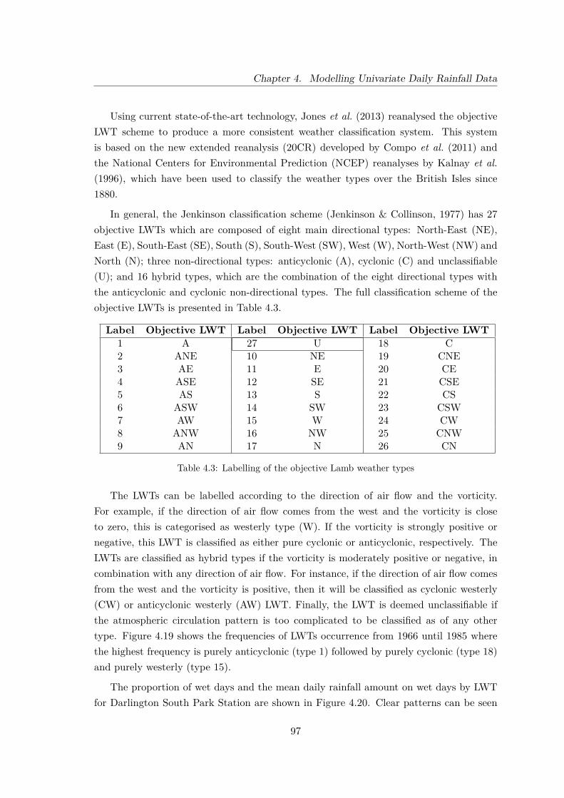
Chapter 4. Modelling Univariate Daily Rainfall Data
Using current state-of-the-art technology, Jones et al. (2013) reanalysed the objectiveLWT scheme to produce a more consistent weather classification system. This systemis based on the new extended reanalysis (20CR) developed by Compo et al. (2011) andthe National Centers for Environmental Prediction (NCEP) reanalyses by Kalnay et al.(1996), which have been used to classify the weather types over the British Isles since1880.
In general, the Jenkinson classification scheme (Jenkinson & Collinson, 1977) has 27objective LWTs which are composed of eight main directional types: North-East (NE),East (E), South-East (SE), South (S), South-West (SW), West (W), North-West (NW) andNorth (N); three non-directional types: anticyclonic (A), cyclonic (C) and unclassifiable(U); and 16 hybrid types, which are the combination of the eight directional types withthe anticyclonic and cyclonic non-directional types. The full classification scheme of theobjective LWTs is presented in Table 4.3.
Label Objective LWT Label Objective LWT Label Objective LWT1 A 27 U 18 C2 ANE 10 NE 19 CNE3 AE 11 E 20 CE4 ASE 12 SE 21 CSE5 AS 13 S 22 CS6 ASW 14 SW 23 CSW7 AW 15 W 24 CW8 ANW 16 NW 25 CNW9 AN 17 N 26 CN
Table 4.3: Labelling of the objective Lamb weather types
The LWTs can be labelled according to the direction of air flow and the vorticity.For example, if the direction of air flow comes from the west and the vorticity is closeto zero, this is categorised as westerly type (W). If the vorticity is strongly positive ornegative, this LWT is classified as either pure cyclonic or anticyclonic, respectively. TheLWTs are classified as hybrid types if the vorticity is moderately positive or negative, incombination with any direction of air flow. For instance, if the direction of air flow comesfrom the west and the vorticity is positive, then it will be classified as cyclonic westerly(CW) or anticyclonic westerly (AW) LWT. Finally, the LWT is deemed unclassifiable ifthe atmospheric circulation pattern is too complicated to be classified as of any othertype. Figure 4.19 shows the frequencies of LWTs occurrence from 1966 until 1985 wherethe highest frequency is purely anticyclonic (type 1) followed by purely cyclonic (type 18)and purely westerly (type 15).
The proportion of wet days and the mean daily rainfall amount on wet days by LWTfor Darlington South Park Station are shown in Figure 4.20. Clear patterns can be seen
97
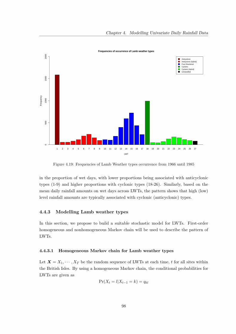
Chapter 4. Modelling Univariate Daily Rainfall Data
1 2 3 4 5 6 7 8 9 10 11 12 13 14 15 16 17 18 19 20 21 22 23 24 25 26 27
Frequencies of occurrence of Lamb weather types
LWT
Fre
qu
en
cy
05
00
10
00
15
00
20
00
AnticyclonicAnticyclonic (hybrid)Pure DirectionalCyclonicCyclonic (hybrid)Unclassified
Figure 4.19: Frequencies of Lamb Weather types occurrence from 1966 until 1985
in the proportion of wet days, with lower proportions being associated with anticyclonictypes (1-9) and higher proportions with cyclonic types (18-26). Similarly, based on themean daily rainfall amounts on wet days across LWTs, the pattern shows that high (low)level rainfall amounts are typically associated with cyclonic (anticyclonic) types.
4.4.3 Modelling Lamb weather types
In this section, we propose to build a suitable stochastic model for LWTs. First-orderhomogeneous and nonhomogeneous Markov chain will be used to describe the pattern ofLWTs.
4.4.3.1 Homogeneous Markov chain for Lamb weather types
Let X = X1, · · · , XT be the random sequence of LWTs at each time, t for all sites withinthe British Isles. By using a homogeneous Markov chain, the conditional probabilities forLWTs are given as
Pr(Xt = l|Xt−1 = k) = qkl
98

Chapter 4. Modelling Univariate Daily Rainfall Data
1 2 3 4 5 6 7 8 9 10 11 12 13 14 15 16 17 18 19 20 21 22 23 24 25 26 27
Mean wet day daily rainfall by Lamb weather type
LWT
Mill
ime
tre
s (m
m)
01
23
45
67
AnticyclonicAnticyclonic (hybrid)Pure DirectionalCyclonicCyclonic (hybrid)Unclassified
(a)
1 2 3 4 5 6 7 8 9 10 11 12 13 14 15 16 17 18 19 20 21 22 23 24 25 26 27
Proportion of wet day by Lamb weather type
LWT
Pro
ba
bili
ty
0.0
0.2
0.4
0.6
0.8
1.0
AnticyclonicAnticyclonic (hybrid)Pure DirectionalCyclonicCyclonic (hybrid)Unclassified
(b)
Figure 4.20: (a) Mean wet day daily rainfall amounts and (b) proportion of wet days by the Lambweather types for Darlington South Park Station
99

Chapter 4. Modelling Univariate Daily Rainfall Data
where state Xt is dependent on Xt−1 and qkl is the transition probability from state k tostate l. Let Q represent the transition matrix for LWTs as:
Q =
q1,1 · · · q1,27
... . . . ...q27,1 · · · q27,27
where
∑27l=1 qkl = 1 and 0 ≤ qkl ≤ 1 with the vector qk representing row k of matrix Q.
Then we can obtain a probability vector π = (π1, π2, · · · , π27) satisfying:
πQ = π
which gives the marginal probabilities when the process is stationary. Subject to cer-tain conditions (see Stewart (2009)), the state probabilities converge to this stationarydistribution as time increases. We can rearrange this equation as:
π(Q− I) = 0 (4.25)
πQ = 0 (4.26)
where I is the identity matrix, 0 is a zero vector and Q = Q−I. By using the informationgiven by
π1 + π2 + · · ·+ π27 = 1,
we can replace the last column of Q and 0 by 1, so that
Q =
q1,1 · · · 1
q2,1. . . 1
......
...q27,1 · · · 1
and 0 = (0, 0, 0, · · · , 1). Hence,
π = 0Q−1. (4.27)
Now, let Nkl represent the observed number of transitions from state k to state l:
N =
N11 · · · N1,27
... . . . ...N27,1 · · · N27,27
100

Chapter 4. Modelling Univariate Daily Rainfall Data
with Nk = (Nk,1, · · · , Nk,27) with nk =∑27l=1Nkl. Then, Nk follows a multinomial distri-
bution:
Nk ∼M27(nk, qk). (4.28)
Let the prior specification for the transition probabilities, qkl, be defined as follows.Let
qkl = eΥkl∑27l=1 e
Υkl.
To avoid a non-identiafiability problem, we set Υkk = 0 for all k = 1, · · · , 27. For Υkl wherek 6= l, we define it as:
Υkl = Υ0l + δkl
where δkl ∼ N(0, υε). To induce general positive correlations between the non-diagonaltransition probabilities and allow borrowing of strength for less-frequent LWTs, we willuse a hierarchical prior as follows:
Υ0l = Υ0 + γl
Υ0 ∼ N(mΥ0, υΥ0
)
γl ∼ N(0, υγ).
Table 4.4 shows an example of posterior means for LWT marginal probabilities using 7305observations of LWTs from 1966 until 1985. The posterior samples were obtained using anMCMC algorithm with 2000 burn-in iterations and subsequent 5000 iterations to obtainthe posterior samples. The computing time that was required to obtain 5000 posteriorsamples was around 2 minutes by using R software on a 2.00GHz Samsung laptop 300V3Amodel with Intel Core i7-2630QM processor and 12 Gbytes of random-access memory.From the table, we can see clearly that type 1 LWT has the highest probability with0.211, where type 2 and 3 LWTs have the lowest probabilities which are 0.08. This resultis consistent with the earlier inference in Figure 4.19.
4.4.3.2 Nonhomogeneous Markov chain of Lamb weather types
Initially, the LWTs are assumed to follow a homogeneous Markov chain. However, thismay not be the case since the frequencies of the different LWTs may depend on the timeof the year resulting in varied LWTs probabilities for every time t. Let the transitionprobabilities for LWTs be given as follows:
Pr(Xt = l|Xt−1 = k) = qkl(t)
101

Chapter 4. Modelling Univariate Daily Rainfall Data
Parameter Mean Parameter Meanπ1 0.211 π15 0.095π2 0.008 π16 0.060π3 0.008 π17 0.033π4 0.012 π18 0.135π5 0.016 π19 0.007π6 0.027 π20 0.007π7 0.032 π21 0.010π8 0.022 π22 0.019π9 0.015 π23 0.025π10 0.015 π24 0.022π11 0.014 π25 0.018π12 0.026 π26 0.015π13 0.053 π27 0.012π14 0.079
Table 4.4: Posterior means of the LWTs probabilties
with a transition matrix of:
Q(t) =
q1,1(t) · · · q1,27(t)
... . . . ...q27,1(t) · · · q27,27(t)
where
∑27l=1 qkl(t) = 1 and 0 ≤ qkl(t) ≤ 1. Since the transition probabilities depend on
time, the process is called a non-homogeneous Markov chain. Given that Xt−1 = k, thestate Xt follows a categorical distribution:
Xt ∼ Cat(qkl(t))
where the transition probabilities qkl(t) are defined to be:
qkl(t) = eΥkl(t)∑27l=1 e
Υkl(t).
Similar to the previous homogeneous process, zero values are assigned to Υkk(t) for allk = 1, · · · , 27 so that the non-identifiability problem can be avoided. In general, the Υkl(t)for k 6= l can be written as
Υkl(t) = Υ0l +F∑f=1
[alfcos
( 2πft365.25
)+ blf sin
( 2πft365.25
)]+ δkl (4.29)
102
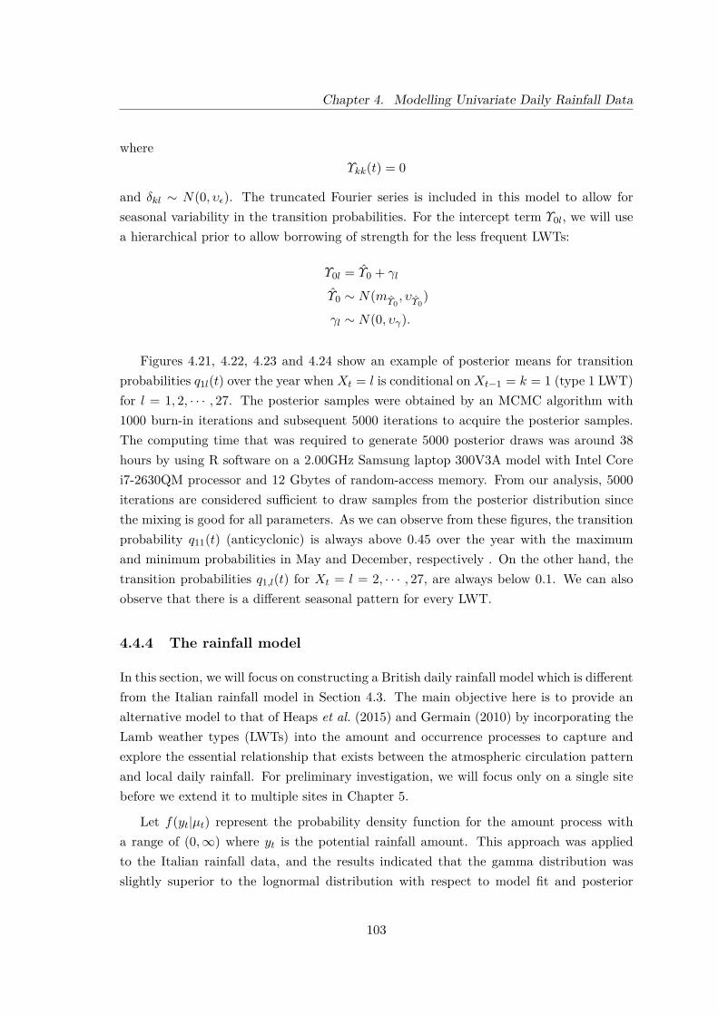
Chapter 4. Modelling Univariate Daily Rainfall Data
whereΥkk(t) = 0
and δkl ∼ N(0, υε). The truncated Fourier series is included in this model to allow forseasonal variability in the transition probabilities. For the intercept term Υ0l, we will usea hierarchical prior to allow borrowing of strength for the less frequent LWTs:
Υ0l = Υ0 + γl
Υ0 ∼ N(mΥ0, υΥ0
)
γl ∼ N(0, υγ).
Figures 4.21, 4.22, 4.23 and 4.24 show an example of posterior means for transitionprobabilities q1l(t) over the year when Xt = l is conditional on Xt−1 = k = 1 (type 1 LWT)for l = 1, 2, · · · , 27. The posterior samples were obtained by an MCMC algorithm with1000 burn-in iterations and subsequent 5000 iterations to acquire the posterior samples.The computing time that was required to generate 5000 posterior draws was around 38hours by using R software on a 2.00GHz Samsung laptop 300V3A model with Intel Corei7-2630QM processor and 12 Gbytes of random-access memory. From our analysis, 5000iterations are considered sufficient to draw samples from the posterior distribution sincethe mixing is good for all parameters. As we can observe from these figures, the transitionprobability q11(t) (anticyclonic) is always above 0.45 over the year with the maximumand minimum probabilities in May and December, respectively . On the other hand, thetransition probabilities q1,l(t) for Xt = l = 2, · · · , 27, are always below 0.1. We can alsoobserve that there is a different seasonal pattern for every LWT.
4.4.4 The rainfall model
In this section, we will focus on constructing a British daily rainfall model which is differentfrom the Italian rainfall model in Section 4.3. The main objective here is to provide analternative model to that of Heaps et al. (2015) and Germain (2010) by incorporating theLamb weather types (LWTs) into the amount and occurrence processes to capture andexplore the essential relationship that exists between the atmospheric circulation patternand local daily rainfall. For preliminary investigation, we will focus only on a single sitebefore we extend it to multiple sites in Chapter 5.
Let f(yt|µt) represent the probability density function for the amount process witha range of (0,∞) where yt is the potential rainfall amount. This approach was appliedto the Italian rainfall data, and the results indicated that the gamma distribution wasslightly superior to the lognormal distribution with respect to model fit and posterior
103
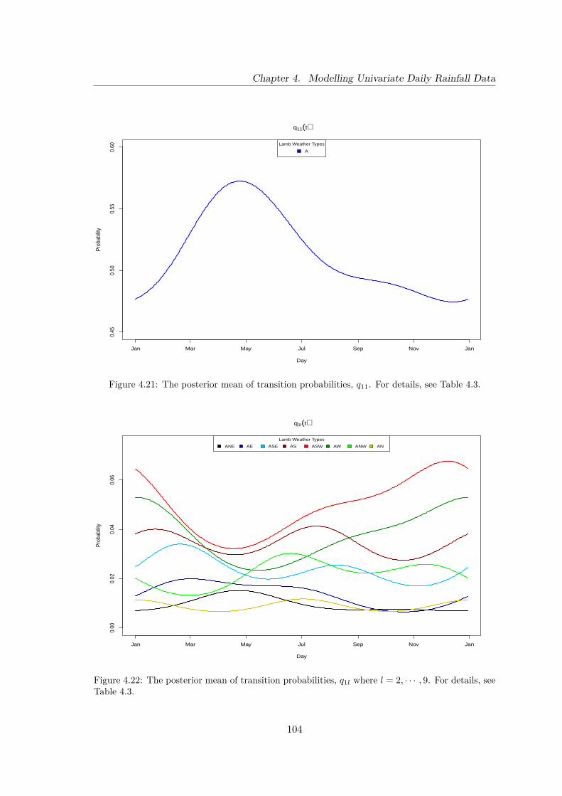
Chapter 4. Modelling Univariate Daily Rainfall Data
Jan Mar May Jul Sep Nov Jan
0.45
0.50
0.55
0.60
q11(t)
Day
Prob
abilit
y
Lamb Weather Types
A
Figure 4.21: The posterior mean of transition probabilities, q11. For details, see Table 4.3.
Jan Mar May Jul Sep Nov Jan
0.00
0.02
0.04
0.06
q1l(t)
Day
Prob
abilit
y
Lamb Weather Types
ANE AE ASE AS ASW AW ANW AN
Figure 4.22: The posterior mean of transition probabilities, q1l where l = 2, · · · , 9. For details, seeTable 4.3.
104

Chapter 4. Modelling Univariate Daily Rainfall Data
Jan Mar May Jul Sep Nov Jan
0.00
0.02
0.04
0.06
0.08
0.10
q1l(t)
Day
Prob
abilit
y
Lamb Weather Types
U NE E SE S SW W NW N
Figure 4.23: The posterior mean of transition probabilities, q1l where l = 10, · · · , 17, 27. Fordetails, see Table 4.3.
Jan Mar May Jul Sep Nov Jan
0.00
00.
005
0.01
00.
015
0.02
0
q1l(t)
Day
Prob
abilit
y
Lamb Weather Types
C CNE CE CSE CS CSW CW CNW CN
Figure 4.24: The posterior mean of transition probabilities, q1l where l = 18, · · · , 26. For details,see Table 4.3.
105
Chapter 4. Modelling Univariate Daily Rainfall Data
predictive performance. From the previous investigation in Section 4.3.3.6, we found thatthe shape parameter did not show significant changes from month to month, while thescale parameter did show some changes over time. Therefore, we propose to use theG1 distribution to describe the potential rainfall amount for the British daily rainfall asfollows:
Yt|α, µt ∼ Ga(α,
α
µt
)where α is the shape parameter, and µt is the mean of the gamma distribution. Forsimplification, we will make the parameter α constant over time. In the case of theamount process, the LWT will be incorporated through the parameter µt. Specifically, letthe parameter µt be modelled using the log link function:
log(µt|xt = k) = ηk0 +F∑f=1
[akfcos
( 2πft365.25
)+ bkf sin
( 2πft365.25
)]+ εt (4.30)
where εt is a random effect at time t. The Fourier series is added to the amount processto capture seasonal variability over the year using three harmonics as indicated in Section4.2.4. The parameter µt is said to be conditional on the LWT by making the intercept,ηk0 , and Fourier coefficients dependent on the LWT at time t. By formulating the ηk0 andFourier coefficients to vary between the LWT, we gain the facility to model the behaviour ofeach LWT. As indicated in Figure 4.20a, we can observe that certain LWTs are associatedwith greater amounts of rainfall than others. Moreover, some of the LWTs might beassociated with greater rainfall at some times of year and less at others. Then, the interceptparameter, ηk0 plays a prominent role in controlling the level of potential rainfall amountswhile Fourier coefficients play a role in accommodating changes in the rainfall amountsassociated with a LWT over the year. In this model, we introduce a random effect in thelinear regression of log(µt) which is assumed to follow a first-order autoregressive modelgiven by
εt = φεεt−1 + ωε
where ωε ∼ N(0, 1/τ). Specifically, this random effect is assumed to follow a normaldistribution:
εt|εt−1 ∼ N(φεεt−1,
1τ
)and the distribution of the random effect at time t = 1 is given by
ε1 ∼ N(
0, 1τ (1− φ2
ε )
)
with |φε| < 1 to ensure stationarity. Then, the mean of the distribution is said to beconditionally dependent on the previous random effect, εt−1. Therefore, the distribution
106
Chapter 4. Modelling Univariate Daily Rainfall Data
of µt is a lognormal distribution. Note that the marginal distribution of Yt given otherparameters obtained by integrating out µt from the joint density of Yt and µt is now nota gamma distribution.
The rainfall occurrence can be modelled using a logit link function and a linear regres-sion to relate the rainfall probabilities to the potential rainfall amount:
logit (p1(t)|xt = k) = ζk0 +F∑f=1
[ckfcos
( 2πf365.25
)+ dkf sin
( 2πf365.25
)]+ ζ1 log(yt) (4.31)
where p0(t) = 1 − p1(t) represents the probability of zero rainfall. This parameterisationis in contrast to the Italian daily rainfall application where we used a nonhomogeneousfirst-order Markov chain to generate the probability of rainfall. As in the amount process,ζk0 is regarded as an intercept parameter for the probability of rainfall with a Fourierseries to allow for seasonal variability where the information of the LWT is incorporatedthrough these parameters. Three harmonics of the Fourier series will be used to representthe seasonal effect of the rainfall amount over the year as suggested in Section 4.2.4.
There are various ways we can use to build the relationship between the amount andoccurrence processes. For example, we can use the mean of the amount distribution,µt, as in Sofia (2007) and the previous Italian model to link between the amount andoccurrence processes. In this model, we use a different approach by incorporating thepotential rainfall amount, yt, into Equation (4.31) to build the relationship between theamount and occurrence processes. Based on the preliminary analysis, we found that theparameters in the occurrence process are well identified when we use yt rather than µt.For instance, Figure 4.25 shows that the posterior density of ζ1 is well identified whenwe used yt instead of µt. Hence, we decided to use the potential rainfall amount, yt as abridge to link between the amount and occurrence processes. The resulting structure isshown in the DAG in Figure 4.26. This figure illustrates the detail of temporal dependencestructure for the univariate model in the context of the British data which is different fromthe previous univariate model.
The parameterisations used for both the amount and occurrence processes are reason-able to model British daily rainfall. However, the model contains a very large number ofparameters since we have many parameters for every single LWT. Therefore, we decided tomodify our model to avoid any difficulties caused by this. The model for both the amountand occurrence process can be simplified by allowing only the intercept parameters ηk0 andζk0 to depend on the LWT while the Fourier coefficients are constant over LWT. Thus, thenew models for rainfall amounts and occurrences are given by
107
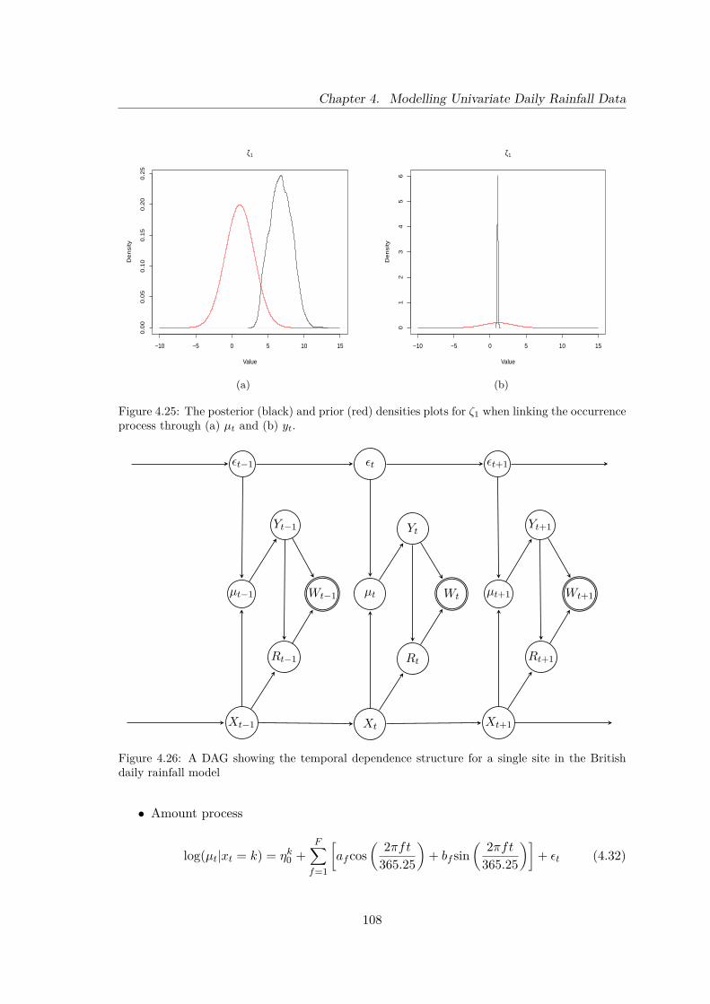
Chapter 4. Modelling Univariate Daily Rainfall Data
−10 −5 0 5 10 15
0.0
00
.05
0.1
00
.15
0.2
00
.25
ζ1
Value
De
nsity
(a)
−10 −5 0 5 10 15
01
23
45
6
ζ1
Value
De
nsity
(b)
Figure 4.25: The posterior (black) and prior (red) densities plots for ζ1 when linking the occurrenceprocess through (a) µt and (b) yt.
εtεt−1 εt+1
µtµt−1 µt+1WtWt−1 Wt+1
YtYt−1 Yt+1
RtRt−1 Rt+1
XtXt−1 Xt+1
Figure 4.26: A DAG showing the temporal dependence structure for a single site in the Britishdaily rainfall model
• Amount process
log(µt|xt = k) = ηk0 +F∑f=1
[afcos
( 2πft365.25
)+ bf sin
( 2πft365.25
)]+ εt (4.32)
108

Chapter 4. Modelling Univariate Daily Rainfall Data
• Occurrence process
logit (p1(t)|xt = k) = ζk0 +F∑f=1
[cfcos
( 2πft365.25
)+ df sin
( 2πft365.25
)]+ ζ1 log(yt).
(4.33)
4.4.4.1 Prior Specifications
This section provides a suggestion for the structure of the prior specifications for theunknown parameters in our model. Normally, the prior distribution is chosen based onthe information acquired from previous studies or personal beliefs. Illustrative values forthe hyperparameters in the prior specifications are given in Section 4.4.5.1.
The shape parameter, α is given a gamma prior distribution:
α ∼ Ga(gα, hα).
A gamma distribution is a sensible prior choice for α since it has only a positive support.The prior distribution for the linear parameters is a normal distribution to allow theparameters to take the values from −∞ to ∞. Then, the prior distribution of the linearparameters for the amount and occurrence processes can be written as follows:
• Amount process
ηk0 ∼N (mη0 , vη0)
af ∼N (ma,f , va,f )
bf ∼N (mb,f , vb,f )
• Occurrence process
ζk0 ∼N (mζ0 , vζ0)
ζ1 ∼N (mζ1 , vζ1)
cf ∼N (mc,f , vc,f )
df ∼N (md,f , vd,f )
where k ∈ {1, 2, · · · , 27} and f ∈ {1, 2, 3}. The Fourier coefficients can be combined as avector for each process as η = (a1, a2, a3, b1, b2, b3)′ and ζ = (c1, c2, c3, d1, d2, d3)′, respec-
109
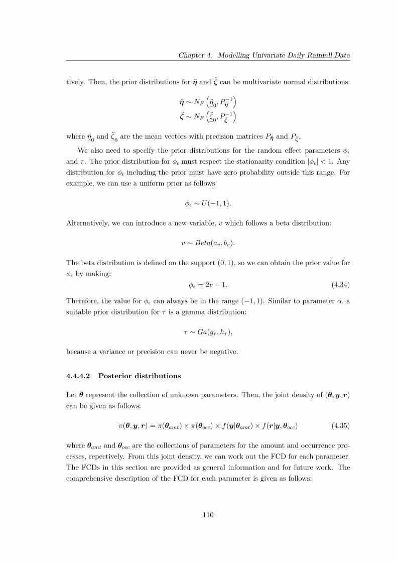
Chapter 4. Modelling Univariate Daily Rainfall Data
tively. Then, the prior distributions for η and ζ can be multivariate normal distributions:
η ∼ NF
(η0, P
−1η
)ζ ∼ NF
(ζ0, P
−1ζ
)where η0 and ζ0 are the mean vectors with precision matrices Pη and Pζ .
We also need to specify the prior distributions for the random effect parameters φεand τ . The prior distribution for φε must respect the stationarity condition |φε| < 1. Anydistribution for φε including the prior must have zero probability outside this range. Forexample, we can use a uniform prior as follows
φε ∼ U(−1, 1).
Alternatively, we can introduce a new variable, v which follows a beta distribution:
v ∼ Beta(av, bv).
The beta distribution is defined on the support (0, 1), so we can obtain the prior value forφε by making:
φε = 2v − 1. (4.34)
Therefore, the value for φε can always be in the range (−1, 1). Similar to parameter α, asuitable prior distribution for τ is a gamma distribution:
τ ∼ Ga(gτ , hτ ),
because a variance or precision can never be negative.
4.4.4.2 Posterior distributions
Let θ represent the collection of unknown parameters. Then, the joint density of (θ,y, r)can be given as follows:
π(θ,y, r) = π(θamt)× π(θocc)× f(y|θamt)× f(r|y,θocc) (4.35)
where θamt and θocc are the collections of parameters for the amount and occurrence pro-cesses, repectively. From this joint density, we can work out the FCD for each parameter.The FCDs in this section are provided as general information and for future work. Thecomprehensive description of the FCD for each parameter is given as follows:
110

Chapter 4. Modelling Univariate Daily Rainfall Data
• Parameter α
The FCD for the shape parameter, α is given by:
π(α|ηk0 , η, v, τ,y) ∝T∏t=1
f(yt|θamt, εt)× π(α)
∝T∏t=1
(α/µt)αyα−1t e−(α/µt)yt
Γ (α) × hgαα αgα−1e−hαα
Γ (gα)
∝(α)αT+gα−1
[Γ (α)]TT∏t=1
Eαt exp{−α
(T∑t=1
Et + hα
)}
where Et = yt/µt. This form does not correspond to any standard distribution.
• Parameter ηk0
Let ηk∗0 =(η1
0, · · · , ηk−10 , ηk+1
0 , · · · , ηK0). With this prior, the FCD for ηk0 is
π(ηk0 |ηk∗0 , α, η, v, τ,y) ∝∏t∈Tk
f(yt|θamt, εt)× π(ηk0 )
∝∏t∈Tk
(α/µt)αyα−1t e−(α/µt)yt
Γ (α) ×√
12πvη0
exp{− 1
2vη0(ηk0 −mη0)2
}
∝∏t∈Tk
Eαt exp{−[α∑t∈Tk
Et + 12vη0
((ηk0 )2 − 2ηk0mη0
) ]}
where Tk = {t : xt = k} is the set of observations for days where the LWT is k.Notice that this FCD does not depend on ηl0, l 6= k and so π(ηk0 |ηk∗0 , α, η, φε, τ,y) =π(ηk0 |α, η, φε, τ,y). The posterior samples can be obtained by taking an independentrealisation from each of π(ηk0 |α, η, φε, τ,y), where k = 1, · · · ,K. However, this FCDdoes not belong to any standard form.
111

Chapter 4. Modelling Univariate Daily Rainfall Data
• Parameter η
The FCD for η is
π(η|α, ηk0 , v, τ,y) ∝T∏t=1
f(yt|θamt, εt)× π(η)
∝T∏t=1
(α/µt)αyα−1t e−(α/µt)yt
Γ (α) × |Pη|1/2
(2π)2F exp{− 1
2(η − η0)′Pη(η − η0)}
∝T∏t=1
Eαt exp{−[α
T∑t=1
Et + 12(η − η0)′Pη(η − η0)
]}.
This is again not in a standard form of any distribution.
• Parameter v
Now, we need to define the FCD for the parameter v as follows:
π(v|ε, τ) ∝f(ε1|τ, φε)T∏t=2
f(εt|εt−1, τ, φε)× π(v)
∝
√τ(1− φ2
ε
)2π exp
{−τ
(1− φ2
ε
)2 ε21
}×
T∏t=2
√τ
2π exp{−τ2 (εt − φεεt−1)2
}
× Γ (av + bv)Γ (av)Γ (bv)
vav−1(1− v)bv−1
∝vav−1(1− v)bv−1√
(1− φ2ε ) exp
{−τ2
[(1− φ2
ε
)ε21 +
T∑t=2
(εt − φεεt−1)2]}
which also does not correspond to any standard distribution.
• Parameter τ
The FCD for the parameter τ is given by
π(τ |ε, v) ∝f(ε1|τ, φε)T∏t=2
f(εt|εt−1, τ, φε)× π(τ)
∝
√τ(1− φ2
ε
)2π exp
{−τ
(1− φ2
ε
)2 ε21
}×
T∏t=2
√τ
2π exp{−τ2 (εt − φεεt−1)2
}
× hgττ τgτ−1e−hτ τ
Γ (gτ )
∝τ gτ+T2 −1 exp
{−τ2
[(1− φ2
ε
)ε21 +
T∑t=2
(εt − φεεt−1)2 + 2hτ
]}.
112

Chapter 4. Modelling Univariate Daily Rainfall Data
This is a gamma distribution Ga(Gτ , Hτ ) with
Gτ = gτ + T
2
and
Hτ = hτ + 12
[(1− φ2
ε
)ε21 +
T∑t=2
(εt − φεεt−1)2].
• Random effect εt
To obtain the sampled values for the random effect εt, the FCD for εt is givenby:
π(εt|τ, φε, yt) ∝f(yt|θamt, εt)× π(εt|εt−1)× π(εt+1|εt)
∝(α/µt)αyα−1t e−(α/µt)yt
Γ (α) ×√τ
2π exp{−τ2 (εt − φεεt−1)2
}×√τ
2π exp{−τ2 (εt+1 − φεεt)2
}∝Eαt exp
{−[αEt + τ
2[(εt − φεεt−1)2 + (εt+1 − φεεt)2
]]}for 1 < t < T − 1. For t = 1, the FCD is given by:
π(ε1|τ, φε, y1) ∝f(y1|θamt, ε1)× π(ε1)× π(ε2|ε1)
∝(α/µ1)αyα−11 e−(α/µ1)y1
Γ (α) ×
√τ(1− φ2
ε
)2π exp
{−τ
(1− φ2
ε
)2 ε21
}
×√τ
2π exp{−τ2 (ε2 − φεε1)2
}∝Eα1 exp
{−[αE1 + τ
2[(
1− φ2ε
)ε21 + (ε2 − φεε1)2
]]}and the FCD for εT is
π(εT |τ, φε, yT ) ∝f(yT |θamt, εT )× π(εT |εT−1)
(α/µT )αyα−1T e−(α/µT )yT
Γ (α) ×√τ
2π exp{−τ2 (εT − φεεT−1)2
}∝EαT exp
{−[αET + τ
2[(εT − φεεT−1)2
]]}.
113
Chapter 4. Modelling Univariate Daily Rainfall Data
• Parameter ζ0
Let ζk∗0 =(ζ1
0 , · · · , ζk−10 , ζk+1
0 , · · · , ζK0). Therefore, the FCD for ζk0 is given by
π(ζk0 |ζk∗0 , ζ1, ζ, r) ∝∏t∈Tk
f(rt|yt,θocc)× π(ζk0 )
∝∏t∈Tk
[p1(t)]rt [1− p1(t)](1−rt) ×√
12πvζ0
exp{− 1
2vζ0
(ζk0 −mζ0)2}
∝∏t∈Tk
[p1(t)]rt [1− p1(t)](1−rt) exp{− 1
2vζ0
(ζk0
)2− 2ζk0mζ0
}.
This distribution is not in a standard form. Notice that this FCD does not dependon ζ l0, l 6= k and so π(ζk0 |ζk∗0 , ζ1, ζ, r) = π(ζk0 |, ζ1, ζ, r). We can sample the posteriorvalue by taking an independent realisation from each of π(ζk0 |, ζ1, ζ, r), where k =1, · · · , 27.
• Parameter ζ1
Next, the FCD for ζ1 is
π(ζ1|ζk0 ζ, r) ∝T∏t=1
f(rt|yt,θocc)× π(ζ1)
∝T∏t=1
[p1(t)]rt [1− p1(t)](1−rt) ×√
12πvζ1
exp{− 1
2vζ1
(ζ1 −mζ1)2}
∝T∏t=1
[p1(t)]rt [1− p1(t)](1−rt) exp{− 1
2vζ1
(ζk1
)2− 2ζk1mζ1
}
where the form indicates that it does not belong to any standard distribution.
• Parameter ζ
For parameter ζ, the FCD can be obtained as follows:
π(ζ|ζk0 , ζ1, z) ∝T∏t=1
f(rt|yt,θocc)× π(ζ)
∝T∏t=1
[p1(t)]rt [1− p1(t)](1−rt) ×|Pζ |1/2
(2π)3 exp{− 1
2(ζ − ζ0)′Pζ(ζ − ζ0)}
∝T∏t=1
[p1(t)]rt [1− p1(t)](1−rt) exp{− 1
2(ζ − ζ0)′Pζ(ζ − ζ0)}.
114

Chapter 4. Modelling Univariate Daily Rainfall Data
Once again, this distribution does not belong to any standard form.
• Latent y-values: ydry
The latent value, yt is not observed when it is a dry day (Wt = 0) which can bedefined as ydry. The values of ydry are treated as auxiliary data in a data augmenta-tion process (Tanner & Wong, 1987). Then, it is necessary to sample the posteriorvalue of ydry when rt = 0 by considering the FCD as follows:
π(ydry|rt = 0, α, µt) ∝f(ydry|α, µt)× Pr(rt = 0|ydry)
∝(α/µt)αyα−1
dry e−(α/µt)ydry
Γ (α) × p0(t)
where p0(t) = 1 − p1(t) represents the probability of a dry day (rt = 0) which alsodepends on ydry.
As we can see, the distributions of most parameters are not in a standard form. Hence,we need to use a Metropolis-within-Gibbs scheme to generate posterior samples for eachparameter. The detailed steps of the MCMC scheme for drawing posterior samples aregiven as follow:
1. Initialise the iteration counter to j=1. Set the initial state of the chain to θ(0) =(α(0), η
1(0)0 , · · · , η27(0)
0 , η(0), v(0), τ (0), ε(0)t , ζ
1(0)0 , · · · , ζ27(0)
0 , ζ(0)1 , ζ(0), ydry
)′.
2. Obtain a new value θ(j) from θ(j−1) by successive generation of values
• α(j) ∼ π(α∣∣∣η1(j−1)
0 , · · · , η27(j−1)j−1 , η(j−1), v(j−1), τ (j−1), ε
(t−1)t , ζ
1(j−1)0 , · · · , ζ27(j−1)
0 ,
ζ(j−1)1 , ζ(j−1),y,x
)using a Metropolis-Hastings step with proposal distribution:
α∗ ∼ Ga(hα∗α
(j−1), hα∗).
• η1(j)0 ∼ π
(η1
0
∣∣∣α(j), η2(j−1)0 , · · · , η27(j−1)
0 , η(j−1), v(j−1), τ (j−1), ε(t−1)t , ζ
1(j−1)0 , · · · ,
ζ27(j−1)0 , ζ
(j−1)1 , ζ(j−1),y,x
)using a Metropolis-Hastings step with proposal dis-
tribution:η1∗
0 ∼ N(η
1(j−1)0 , Ση∗0
)with a suitable variance, Ση∗0 .
...
115

Chapter 4. Modelling Univariate Daily Rainfall Data
• η27(j)0 ∼ π
(η27
0
∣∣∣α(j), η1(j)0 , · · · , η26(j)
0 , η(j−1), v(j−1), τ (j−1), ε(j−1)t , ζ
1(j−1)0 , · · · ,
ζ27(j−1)0 , ζ
(j−1)1 , ζ(j−1),y,x
)using a Metropolis-Hastings step with proposal dis-
tribution:η27∗
0 ∼ N(η
27(j−1)0 , Ση∗0
).
• η(j) ∼ π(η∣∣∣α(j), η
1(j)0 , · · · , η27(j)
0 , v(j−1), τ (j−1), ε(j−1)t , ζ
1(j−1)0 , · · · , ζ27(j−1)
0 , ζ(j−1)1 ,
ζ(j−1),y,x)
using a Metropolis-Hastings step with proposal distribution:
η∗ ∼ N6(η(j−1), Ση∗
).
• v(j) ∼ π(v∣∣∣α(j), η
1(j)0 , · · · , η27(j)
0 , η(j), τ (j−1), ε(j−1)t , ζ
1(j−1)0 , · · · , ζ27(j−1)
0 , ζ(j−1)1 ,
ζ(j−1),y,x)
using a Metropolis-Hastings step with proposal distribution:
v∗ ∼ Beta(bv∗v
(j−1), bv∗(1− v(j−1)
)).
• τ (j) ∼ π(τ∣∣∣α(j), η
1(j)0 , · · · , η27(j)
0 , η(j), v(j), ε(j−1)t , ζ
1(j−1)0 , · · · , ζ27(j−1)
0 , ζ(j−1)1 ,
ζ(j−1),y,x)
using a Gibbs sampler step where
τ∗ ∼ Ga (Gτ , Hτ ) .
• ε(j)t ∼ π(εt∣∣∣α(j), η
1(j)0 , · · · , η27(j)
0 , η(j), v(j), τ j , ζ1(j−1)0 , · · · , ζ27(j−1)
0 , ζ(j−1)1 , ζ(j−1),y
)using a Metropolis-Hastings step with proposal distribution:
ε∗t ∼ N(ε(j−1)t , σ2
ε∗
)with a suitable variance, σ2
ε∗ . For example σ2ε∗ = [τ(1− φ2
ε )]−1.
• ζ1(j)0 ∼ π
(ζ1
0
∣∣∣α(j), η1(j)0 , · · · , η27(j)
0 , η(j), v(j), τ (j), ε(j)t , ζ
2(j−1)0 , · · · , ζ27(j−1)
0 , ζ(j−1)1 ,
ζ(j−1),y,x)
using a Metropolis-Hastings step with proposal distribution:
ζ1∗0 ∼ N
(ζ
1(j−1)0 , Σζ∗0
).
...
• ζ27(j)0 ∼ π
(ζ27
0
∣∣∣α(j), η1(j)0 , · · · , η27(j)
0 , η(j), v(j), τ (j), ε(j)t , ζ
1(j)0 , · · · , ζ26(j)
0 , ζ(j−1)1 ,
ζ(j−1),y,x)
using a Metropolis-Hastings step with proposal distribution:
116
Chapter 4. Modelling Univariate Daily Rainfall Data
ζ27∗0 ∼ N
(ζ
27(j−1)0 , Σζ∗0
).
• ζ(j)1 ∼ π
(ζ1∣∣∣α(j), η
1(j)0 , · · · , η27(j)
0 , η(j), v(j), τ (j), ε(j)t , ζ
1(j)0 , · · · , ζ27(j)
0 , ζ(j−1),y,x)
using a Metropolis-Hastings step with proposal distribution:
ζ∗1 ∼ N(ζ
(j−1)1 , Σζ∗1
).
• ζ(j) ∼ π(ζ∣∣∣α(j), ζ
1(j)0 , · · · , ζ27(j)
0 , η(j), v(j), τ (j), ε(j)t , ζ
1(j)0 , · · · , ζ27(j)
0 , ζ(j)1 ,y,x
)using a Metropolis-Hastings step with proposal distribution:
ζ∗ ∼ N6(ζ(j−1), Σζ∗
).
• y(j)dry ∼ π
(ydry
∣∣∣α(j), ζ1(j)0 , · · · , ζ27(j)
0 , η(j), v(j), τ (j), ε(j)t , ζ
1(j)0 , · · · , ζ27(j)
0 , ζ(j)1 , ζ(j),
y,x)
3. Change counter j to j + 1, and return to step 2.
4.4.5 Application
4.4.5.1 Prior distribution
The prior specifications for the British daily rainfall model were constructed using suitabledistributions based on the information gained from previous studies and personal beliefs.The chosen prior structure for this model and the methods of elicitation are intended asrecommendations. The actual choice of hyperparameters here is for illustrative purposesonly.
In the British daily rainfall model we use the G1 distribution for the rainfall amount.However the situation is more complicated for two reasons. The first is that we do notobserve samples from the distribution of Yt. We only observe samples from the distributionof Wt. The second is the presence of the random effect εt in (4.32). Pragmatically forelicitation purposes, we propose to ignore the first problem and elcit beliefs about observedrainfall amounts and to approximate the distribution of the rainfall amount Yt with alognormal distribution. So, approximately, Zt = log Yt has a normal distribution.
Suppose that we writeZt = η?t + et + εt
where et ∼ N(0, ve), εt ∼ N(0, vε) and vε = [τ(1 − φ2ε )]−1. Then the expectation of Yt,
117
Chapter 4. Modelling Univariate Daily Rainfall Data
given model parameters and the LWT, is
E(Yt | xt = k, ηt) = exp{η?t + (ve + vε)/2}.
So we writelog{E(Yt | xt = k, ηt)} = ηt = η?t + (ve + vε)/2
where, from (4.32),
η?t = ηk0 +F∑f=1
[af cos
( 2πft365.25
)+ bf sin
( 2πft365.25
)].
To find the marginal prior distribution of η?t = E(Zt) we can use the first part of themethod for the lognormal distribution in Section 4.3.3.1, and questions Q11, Q12 andQ13.
To elicit beliefs about ve, τ and φε, we need to consider rainfall on, at least, threewet days, t, t − k1 and t − k2, where, for example, k1 = 1 and k2 = 3. Given the modelparameters and LWT, the log rainfall amounts, Zt, Zt−k1 and Zt−k2 on these days haveapproximately a multivariate normal distribution. Al-Awadhi & Garthwaite (1998, 2001)describe a method for eliciting prior distributions for the parameters of multivariate normaldistributions. However, in our case, the multivariate normal distributions has a specific,time-series, structure which does not correspond well with this method. We proposeinstead that the expert is asked to imagine a large number of replications of sequencesof wet days at a similar time of year and under the same atmospheric conditions. Thevariance of Zt is ve + vε. The covariance of Zt and Zt−k is φkε vε. The correspondingcorrelation is
Corr(Zt,Zt−k) = φkεvε
ve + vε.
The expert’s quartiles for the corresponding sample covariances from a large numberof replications can be elicited. Alternatively, the correlation may be expressed in termsof the reduction in conditional variance of Zt given knowledge of Zt−k. We then give theparameters distributions as follows:
τ ∼ Ga(gτ , hτ ),
α = [exp(ve)− 1]−1 ∼ Ga(gα, hα), (4.36)
v = (φε + 1)/2 ∼ Beta(av, bv).
The hyperparameters gτ , hτ , gα, hα, av and bv are varied iteratively until the specified quar-tiles for the variance and covariances are reasonably matched by the implied quartiles
118
Chapter 4. Modelling Univariate Daily Rainfall Data
which are numerically computed. The relationship α = [exp(ve) − 1]−1 in (4.36) arisesfrom considering the case where εt = 0, in which case
E(Yt | εt = 0) = exp{η?t + ve/2} = α/β and
Var(Yt | εt = 0) = exp{2η?t + ve}(exp{ve} − 1) = α/β2.
For illustration, we have chosen carefully suitable values for the hyperparameters ofthe unknown parameters in the amount process using the above methods as follows:
mA0 = 0.69, vA0 = 4.22,
gα = 4.31, hα = 5.78,
gτ = 3.69, hτ = 1.68,
av = 3.7, bv = 1.9.
As in Section 4.3.3.3, we can elicit beliefs about rainfall amounts at several differenttimes of year in order to develop a prior distribution for the Fourier coefficients. In ourillustration we use the same values as used there.
The prior specification for the unknown parameters of the occurrence process is morecumbersome. However we can use a method similar to that in Section 4.3.3.2. If weconsider rainfall occurence on a day of the year when we believe that the seasonal effectsin (4.33) will cancel out, we might then represent the occurrence process using a simplelogistic regression:
logit(p) = log(
p
1− p
)= ζ0 + ζ1 log(y).
The second term on the right hand side has two effects which are observable, at leastin theory. Firstly it causes a change in the distribution of observed rainfall amounts butdirect prior beliefs about such a subtle change are unlikely to be reliably elicited. Secondly,because Yt and Yt−1 are autocorrelated, it causes dependence between successive rainfalloccurrences. However this relationship is somewhat complicated.
Our approach is as follows. We substitute log Yt = η?t +et+εt. Then, as a first step, weconsider different values of η?t with et and εt assumed to be zero. We use a similar approachas in Questions Q22 and Q23 in Section 4.3.3.2 to elicit a prior for unknown parametersin the occurrence process in this situation. In this case, though, we do not condition onit having rained on the preceding day. It is then possible to refine the elicitation by usingan iterative numerical procedure considering the effect of the distribution of et and εt. We
119
Chapter 4. Modelling Univariate Daily Rainfall Data
have chosen carefully two different scenarios for illustration as follows:
Kp1 = logit(p1) = ζ0 + log(0.2)ζ1,
Kp2 = logit(p2) = ζ0 + log(0.6)ζ1
where we assess that
Pr(p1 < 0.139) = Pr(p1 > 0.432) = 0.25,
Pr(p2 < 0.335) = Pr(p2 > 0.806) = 0.25.
Suppose that Kp1 ∼ N(mKp1 , σ2Kp1
). From the specification for p1 we have
Pr(Kp1 < logit 0.139 = −1.824) = 0.25,
Pr(Kp1 > logit 0.432 = −0.274) = 0.25
and using the properties of the normal distribution, we can get
mKp1 − 0.674σKp1 = −1.824, mKp1 + 0.674σKp1 = −0.274
where mKp1 = (−1.824−0.274)/2 = −1.049 and σ2Kp1
= [(1.824−0.274)/2×0.674]2 = 1.33.Similar calculations are given to Kp2 where we have
Kp1 ∼ N(−1.05, 1.33)
Kp2 ∼ N(0.37, 2.44).
Suppose that Kp1 and Kp2 is independent and therefore this can be summarised as follows:
E(ζ0 − 1.6094ζ1) = −1.05
E(ζ0 − 0.5108ζ1) = 0.37
and
Var(ζ0 − 1.6094ζ1) = 1.33
Var(ζ0 − 0.5108ζ1) = 2.44
Cov(ζ0 − 1.6094ζ1, ζ0 − 0.5108ζ1) = 0.
120
Chapter 4. Modelling Univariate Daily Rainfall Data
By solving the linear equations above, we obtain(E(ζ0)E(ζ1)
)=(
1.031.29
)
and (Var(ζ0) Cov(ζ0, ζ1)
Cov(ζ0, ζ1) Var(ζ1)
)=(
5.52 3.823.82 3.12
).
We can use the method of Section 4.3.3.3 to determine a prior distribution for theFourier coefficients.
4.4.5.2 Fitting the model
The Rjags package (Plummer, 2012) is used to compute the posterior samples for thismodel. The MCMC algorithm was run for 10000 iterations to allow for burn-in, and anadditional 150000 iterations were obtained as the posterior samples. The computing timethat was used to obtain 150000 posterior draws was around 38 hours by using R softwareon a 3.40GHz Ergo Desktop AS4 All-in-One with Intel Core i7-3770 processor and 8 Gbytesof random-access memory. The trace plots can be used as a visual diagnostic to monitorthe convergence of the sampler. In this model, the trace plots for all parameters wereconsidered before we make any inferences or conclusions. Figure 4.27 displays the exampleof trace plots and posterior density of the parameters for the Anticyclonic type (type 1)with some other parameters. An issue that has to be considered when using MCMCmethods is that the sample values from the stationary distribution are not independent.The trace plots in Figure 4.27, for the parameters α and τ indicate that these parametershave a relatively high autocorrelation, which suggests mixing is slow. The chain movesmore slowly around the distribution, and so more samples are required. Thus, 150000iterations were considered necessary to draw posterior samples. Poor mixing can affectposterior summary statistics, and obviously we want the sampled numerical summariesto be as close to the true posterior values as possible. We can observe that the samplesfor the other parameters are not as strongly autocorrelated and the mixing is good inthe same figure. The uncertainty associated with most of the unknown parameters hasbeen reduced after we combined the prior beliefs with the data. For example, there is areduction in the variability of parameter ζ1 when a comparison is made between the priorand posterior distributions. The posterior mean of parameter ζ1 is shifted to the left ofits prior mean. The full summaries of posterior means and standard deviations of theunknown parameters for the amount and occurrence processes are given in Table 4.5 and4.6.
121

Chapter 4. Modelling Univariate Daily Rainfall Data
Figure 4.27: The trace and density plots for parameters α, η10 , τ , v, ζ1
0 and ζ1
122

Chapter 4. Modelling Univariate Daily Rainfall Data
Amount processParameter Prior mean Prior SD Posterior mean Posterior SDα 0.75 0.36 0.717 0.056η1
0 0.69 2.05 -0.411 0.085η2
0 0.69 2.05 0.776 0.236η3
0 0.69 2.05 0.125 0.253η4
0 0.69 2.05 -0.229 0.241η5
0 0.69 2.05 -0.756 0.226η6
0 0.69 2.05 -0.735 0.188η7
0 0.69 2.05 -0.395 0.147η8
0 0.69 2.05 0.392 0.164η9
0 0.69 2.05 0.305 0.186η10
0 0.69 2.05 0.846 0.163η11
0 0.69 2.05 0.531 0.179η12
0 0.69 2.05 -0.045 0.159η13
0 0.69 2.05 -0.452 0.128η14
0 0.69 2.05 -0.030 0.093η15
0 0.69 2.05 0.074 0.081η16
0 0.69 2.05 0.410 0.093η17
0 0.69 2.05 1.140 0.118η18
0 0.69 2.05 1.116 0.066η19
0 0.69 2.05 1.354 0.244η20
0 0.69 2.05 1.093 0.250η21
0 0.69 2.05 0.875 0.210η22
0 0.69 2.05 0.448 0.158η23
0 0.69 2.05 0.541 0.137η24
0 0.69 2.05 0.773 0.136η25
0 0.69 2.05 1.006 0.152η26
0 0.69 2.05 1.258 0.170η27
0 0.69 2.05 0.339 0.203a1 0 0.80 0.033 0.044a2 0 0.56 0.049 0.042a3 0 0.46 0.011 0.042b1 0 0.80 -0.106 0.041b2 0 0.56 -0.001 0.042b3 0 0.46 0.011 0.042τ 2.2 1.14 1.967 0.328v 0.66 0.18 0.803 0.021
Table 4.5: The prior and posterior means with standard deviations (SD) of the unknown parametersfor the amount process
123

Chapter 4. Modelling Univariate Daily Rainfall Data
Occurrence processParameter Prior mean Prior SD Posterior mean Posterior SDζ1
0 1.03 2.35 -0.256 0.131ζ2
0 1.03 2.35 0.414 0.401ζ3
0 1.03 2.35 0.717 0.410ζ4
0 1.03 2.35 -0.150 0.359ζ5
0 1.03 2.35 0.077 0.337ζ6
0 1.03 2.35 -0.220 0.272ζ7
0 1.03 2.35 0.181 0.228ζ8
0 1.03 2.35 0.047 0.253ζ9
0 1.03 2.35 0.516 0.304ζ10
0 1.03 2.35 1.423 0.324ζ11
0 1.03 2.35 1.170 0.314ζ12
0 1.03 2.35 0.337 0.247ζ13
0 1.03 2.35 0.157 0.186ζ14
0 1.03 2.35 0.530 0.151ζ15
0 1.03 2.35 0.651 0.145ζ16
0 1.03 2.35 1.029 0.179ζ17
0 1.03 2.35 1.222 0.239ζ18
0 1.03 2.35 1.291 0.137ζ19
0 1.03 2.35 0.659 0.490ζ20
0 1.03 2.35 1.247 0.521ζ21
0 1.03 2.35 1.011 0.395ζ22
0 1.03 2.35 0.938 0.285ζ23
0 1.03 2.35 1.175 0.262ζ24
0 1.03 2.35 1.262 0.269ζ25
0 1.03 2.35 1.378 0.312ζ26
0 1.03 2.35 1.179 0.358ζ27
0 1.03 2.35 0.906 0.348c1 0 0.80 0.369 0.054c2 0 0.56 -0.034 0.053c3 0 0.46 0.005 0.053d1 0 0.80 0.107 0.053d2 0 0.56 0.104 0.053d3 0 0.46 -0.037 0.053ζ1 1.29 1.77 1.060 0.068
Table 4.6: The prior and posterior means with standard deviations (SD) of the unknown parametersfor the occurrence process
124

Chapter 4. Modelling Univariate Daily Rainfall Data
−1.0
−0.5
0.0
0.5
1.0
1.5
η0k
Type
Valu
e
1 2 3 4 5 6 7 8 9 10 11 12 13 14 15 16 17 18 19 20 21 22 23 24 25 26 27
Figure 4.28: The posterior mean with 95% credible intervals for ηk0 where k ∈ {1, · · · , 27}
−0.5
0.0
0.5
1.0
1.5
2.0
ζ0k
Type
Valu
e
1 2 3 4 5 6 7 8 9 10 11 12 13 14 15 16 17 18 19 20 21 22 23 24 25 26 27
Figure 4.29: The posterior mean with 95% credible intervals for ζk0 where k ∈ {1, · · · , 27}
125

Chapter 4. Modelling Univariate Daily Rainfall Data
Figure 4.28 shows the posterior mean and 95% credible intervals of the parameterηk0 for every type k ∈ {1, · · · , 27}. In this figure, the cyclonic types (18-26) have largerposterior means of ηk0 with the means being greater than 0.5. This finding is consistentwith the early inference as shown in Figure 4.20a. The LWTs thus play an important rolein influencing the quantity of rainfall. For example, the cyclonic type might produce agreater rainfall amount than other types over a year. Also, the previous random effect attime t−1 is also vital in determining the level of the rainfall amount at time t. It is highlypossible that the rainfall amount will increase if the rainfall does occur on the previousday. Figure 4.29 shows that the posterior mean of ζk0 varies between types k ∈ {1, · · · , 27},and thus the LWT will determine the rainfall probability at time t. This can be illustratedby referring to the Figure 4.20b where the cyclonic types are associated with the greatestlevels of rainfall probability which is also consistent with the early inference.
FDT residuals
Value
Freq
uenc
y
0.0 0.2 0.4 0.6 0.8 1.0
040
80
0 200 400 600
−20
2
NFT residuals
Time
Value
Figure 4.30: The FDTR and NFTR plots for British daily rainfall
Section 4.2.6 describes the diagnostic checking methods used for the mixed distributionbased on Smith (1985). Therefore, we will use this approach to assess the adequacy of ourmodel by generating the posterior mean of the FDTR and NFTR from year 1967 until1968. The graphs of these residuals are shown in Figure 4.30. In these figures, we canobserve that these residuals conform to the respective series of independent uniform andindependent normal observations. We can further examine the model by looking at thequantile-quantile (QQ), ACF and PACF plots for the NFTR in Figure 4.31. The linearityof the points in the QQ plot indicates that the NFTR are normally distributed. The ACFand PACF plots demonstrate that the residuals are not highly correlated. The evidencefrom the plots suggests that the model fits the data very well.
126
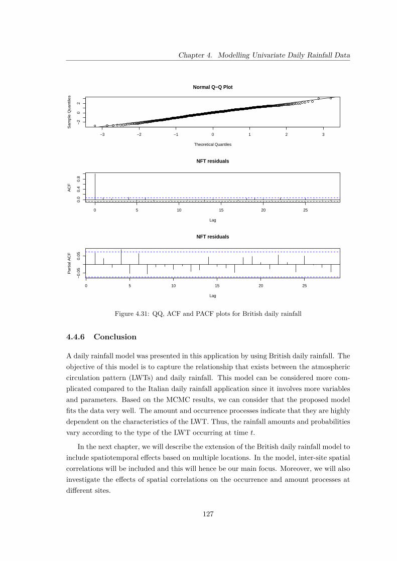
Chapter 4. Modelling Univariate Daily Rainfall Data
−3 −2 −1 0 1 2 3
−2
02
Normal Q−Q Plot
Theoretical Quantiles
Sa
mp
le Q
ua
ntil
es
0 5 10 15 20 25
0.0
0.4
0.8
Lag
AC
F
NFT residuals
0 5 10 15 20 25
−0
.05
0.0
5
Lag
Pa
rtia
l AC
F
NFT residuals
Figure 4.31: QQ, ACF and PACF plots for British daily rainfall
4.4.6 Conclusion
A daily rainfall model was presented in this application by using British daily rainfall. Theobjective of this model is to capture the relationship that exists between the atmosphericcirculation pattern (LWTs) and daily rainfall. This model can be considered more com-plicated compared to the Italian daily rainfall application since it involves more variablesand parameters. Based on the MCMC results, we can consider that the proposed modelfits the data very well. The amount and occurrence processes indicate that they are highlydependent on the characteristics of the LWT. Thus, the rainfall amounts and probabilitiesvary according to the type of the LWT occurring at time t.
In the next chapter, we will describe the extension of the British daily rainfall model toinclude spatiotemporal effects based on multiple locations. In the model, inter-site spatialcorrelations will be included and this will hence be our main focus. Moreover, we will alsoinvestigate the effects of spatial correlations on the occurrence and amount processes atdifferent sites.
127
Chapter 4. Modelling Univariate Daily Rainfall Data
4.5 Summary
In this chapter, we have described the construction of a general daily rainfall model for asingle site within the Bayesian framework. Modelling daily rainfall can be quite challengingsince there is a mixture of discrete and continuous components in the data. In the generalmodel, we have emphasised the relationship between the amount and occurrence processesusing a two-stage approach as shown in Section 4.2. We have also described methods thatwe can use to construct a model for the amount and occurrence processes in Sections 4.2.2and 4.2.3. An important novelty in this study is dealing with seasonal effects as the dataobtained spans the whole year. We have introduced two different types of Fourier seriesin Section 4.2.4 to take into account the seasonal variability over a year. Then, we appliedthis general model to the Italian and British datasets.
For the Italian daily rainfall application in Section 4.3, we have proposed to use threedifferent distributions for the amount process: lognormal distribution, G1 distribution andG2 distribution (for details, see Section 4.3.2.1). From these three distributions, it wasfound that both the G1 and G2 distributions fitted the data slightly better compared to alognormal distribution based on the posterior mean for the mean of the potential rainfallamount and posterior predictive values. Since both G1 and G2 distributions are gammadistributions, we can observe that the gamma distribution is a better choice for the amountprocess modelling for the Italian rainfall data. Furthermore, we have discovered that theshape parameter does not change noticeably over the year while the scale parameter hasclear-cut shifts as comparisons were made from month to month as shown in Section4.3.3.6. For the occurrence process, we have used a first-order Markov chain to fit therainfall occurrence where the rainfall occurrence at current time t is dependent on that ofthe previous time t− 1. The detailed parameterisation for the occurrence process can befound in Section 4.3.2.2.
We have also built a model for the British daily rainfall which is different from theItalian application by incorporating the atmospheric circulation patterns in the model.In the British model, we have chosen the LWTs to represent the atmospheric circulationpatterns. The LWT is incorporated into the model through the amount and occurrenceprocesses. Our aim for this model is to build an alternative model from the previous workby Heaps et al. (2015) and Germain (2010). These authors used the LWT to characteriseatmospheric circulation patterns by combining it with the weather state process usinga NHMM approach for the UK winter rainfall. This model is entirely different fromour model where we applied the LWT directly to the model instead of using hiddenweather states and a NHMM approach. We believe that the LWT plays a critical rolein determining rainfall amounts and occurrences over the British Isles as we can see in
128

Chapter 4. Modelling Univariate Daily Rainfall Data
Section 4.4.2. Furthermore, we used data from all times of year to generate the Britishdaily rainfall model where the Fourier series is used to allow for seasonal variability in thedata. To build a model for the amount process, we have used a gamma distribution wherewe introduced a random effect at time t which is conditionally dependent on the previoustime t−1. For the occurrence process, we proposed a simple parameterisation to calculatethe probability of rainfall occurrence. As we can see in Section 4.4.4, the parameterisationfor the amount and occurrence processes of the British application is in contrast withthe Italian application. The MCMC results have indicated that the model fits the datavery well as shown in Section 4.4.5.2. It also shows that the level of the potential rainfallamount and the probability of rainfall occurrence are relatively dependent on the typeof LWT. In the next chapter, we will describe the extension of this British daily rainfallmodel with multiple sites.
129

Chapter 5
Spatiotemporal Model for DailyRainfall Data
5.1 Introduction
Following the introduction of the daily rainfall model in Chapter 4, we will now introducea spatiotemporal model which is the extended version of the previous univariate model.The purpose of this chapter is hence to present an alternative spatiotemporal model tothe previous models developed by Heaps et al. (2015) and Germain (2010) who used non-homogeneous hidden Markov models to fit a model for the winter daily rainfall data inthe United Kingdom (UK). In their modelling framework, the atmospheric circulationpatterns were linked to the latent weather states to model their influence on the dailyrainfall pattern. Instead of using hidden weather states, we propose a model in whichwe can directly link the atmospheric circulation patterns to the rainfall occurrences andamounts via the conditional model parameters. We also aim to capture the relationshipthat exists between the sites and investigate how this relationship can affect the dailyrainfall pattern at neighboring sites.
Section 5.2 describes the general information about the spatiotemporal model. Theexploration of the daily rainfall dataset and the spatial characteristics of each location willbe subsequently discussed in Section 5.3. Next, we introduce the spatiotemporal model forUK daily rainfall in Section 5.4. Similar to the univariate model, the Lamb weather types(LWTs) will be incorporated into the model via the amount and occurrence processes.This will lead to a more complex model that requires extensive computational time. Thedetailed prior and posterior distributions for the model are described in Sections 5.5 and5.6, respectively.
130
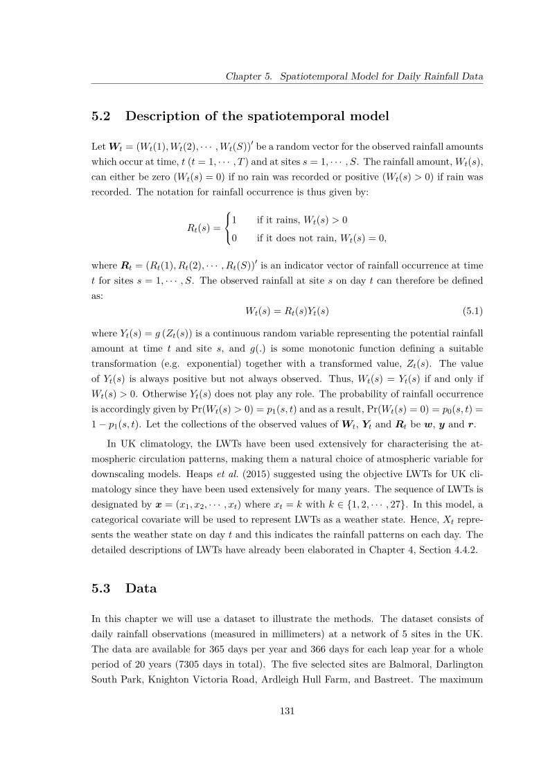
Chapter 5. Spatiotemporal Model for Daily Rainfall Data
5.2 Description of the spatiotemporal model
LetWt = (Wt(1),Wt(2), · · · ,Wt(S))′ be a random vector for the observed rainfall amountswhich occur at time, t (t = 1, · · · , T ) and at sites s = 1, · · · , S. The rainfall amount, Wt(s),can either be zero (Wt(s) = 0) if no rain was recorded or positive (Wt(s) > 0) if rain wasrecorded. The notation for rainfall occurrence is thus given by:
Rt(s) =
1 if it rains, Wt(s) > 0
0 if it does not rain, Wt(s) = 0,
where Rt = (Rt(1), Rt(2), · · · , Rt(S))′ is an indicator vector of rainfall occurrence at timet for sites s = 1, · · · , S. The observed rainfall at site s on day t can therefore be definedas:
Wt(s) = Rt(s)Yt(s) (5.1)
where Yt(s) = g (Zt(s)) is a continuous random variable representing the potential rainfallamount at time t and site s, and g(.) is some monotonic function defining a suitabletransformation (e.g. exponential) together with a transformed value, Zt(s). The valueof Yt(s) is always positive but not always observed. Thus, Wt(s) = Yt(s) if and only ifWt(s) > 0. Otherwise Yt(s) does not play any role. The probability of rainfall occurrenceis accordingly given by Pr(Wt(s) > 0) = p1(s, t) and as a result, Pr(Wt(s) = 0) = p0(s, t) =1− p1(s, t). Let the collections of the observed values of Wt, Yt and Rt be w, y and r.
In UK climatology, the LWTs have been used extensively for characterising the at-mospheric circulation patterns, making them a natural choice of atmospheric variable fordownscaling models. Heaps et al. (2015) suggested using the objective LWTs for UK cli-matology since they have been used extensively for many years. The sequence of LWTs isdesignated by x = (x1, x2, · · · , xt) where xt = k with k ∈ {1, 2, · · · , 27}. In this model, acategorical covariate will be used to represent LWTs as a weather state. Hence, Xt repre-sents the weather state on day t and this indicates the rainfall patterns on each day. Thedetailed descriptions of LWTs have already been elaborated in Chapter 4, Section 4.4.2.
5.3 Data
In this chapter we will use a dataset to illustrate the methods. The dataset consists ofdaily rainfall observations (measured in millimeters) at a network of 5 sites in the UK.The data are available for 365 days per year and 366 days for each leap year for a wholeperiod of 20 years (7305 days in total). The five selected sites are Balmoral, DarlingtonSouth Park, Knighton Victoria Road, Ardleigh Hull Farm, and Bastreet. The maximum
131

Chapter 5. Spatiotemporal Model for Daily Rainfall Data
and minimum distances between the sites in this network are 724.8 km and 221.8 km,respectively. A spatial plot of the network of the measurement sites (i.e. the 5 weatherstations) is given in Figure 5.1.
Longitude
Latit
ude
−8 −6 −4 −2 0 2 4
5052
5456
58
Balmoral
Darlington South Park
Knighton Victoria RoadArdleigh Hull Farm
Bastreet
Figure 5.1: The locations of the United Kingdom weather stations chosen as the measurement sitesfor daily rainfall
As explained in Chapter 4, rainfall data contain zeros and positive values. A dry dayis defined as a day in which the rain does not occur or the rainfall amount is insufficientto meet the standard operational definition of a positive rainfall. For this purpose, we usethe operational definition adopted by the American Meteorological Society which is thata recorded rainfall amount of less than 0.01 inches or 0.2 mm within a 24-hour period isclassified as zero rainfall (Glickman, 2000; Germain, 2010). This cut-off will hence be usedto classify a day as either dry or wet as we scrutinise the British rainfall data.
Table 5.1 shows summaries of the altitude, the proportion of wet days, the meanand maximum daily rainfall amounts for each site. Contingent upon this information, thehighest proportion of wet days were recorded at Bastreet (66.50%) whilst Darlington SouthPark had the smallest proportion (49.39%) of wet days. The mean daily rainfall amount
132

Chapter 5. Spatiotemporal Model for Daily Rainfall Data
Site Altitude(m)
Proportionwet days
(%)
Mean dailyrainfall(mm)
Maxrainfallamount(mm)
1 Balmoral 276.82 60.82 2.33 74.72 Darlington South Park 44.20 49.39 1.84 48.83 Knighton Victoria Road 179.58 65.43 2.75 51.84 Ardleigh Hull Farm 34.09 49.50 1.57 47.15 Bastreet 270.60 66.50 4.65 114.3
Table 5.1: Summary of data from five sites within the UK from 1966 until 1985
ranges from 1.5 mm to 5.0 mm with the highest mean daily rainfall amount recorded atBastreet. In addition, the daily rainfall amount may also reach up to nearly 115 mm for aparticular site such as Bastreet which recorded a maximal daily rainfall amount of 114.3mm over the 20-year observation period.
Figure 5.2 depicts the mean daily rainfall amounts on the wet days and the proportionsof wet days classified according to the LWTs for all sites. We can observe that the highamounts of daily rainfall in Figure 5.2a are associated with the cyclonic types whereas thelow daily rainfall amounts are related to the anticyclonic types. A similar pattern can alsobe evidently seen for the proportions of wet days (Figure 5.2b), where a higher probabilityof rain occurrence is associated with the cyclonic types whilst the anticyclonic types areassociated with a lower probability of rainfall occurrence.
We can also investigate the spatial structure of the daily rainfall pattern to evaluatewhether similar rainfall characteristics are observed between sites. For this endeavour,we take heed of the recommendations made by Germain (2010). Hence, we used theSpearman’s rank correlation and log odds ratio to assess the spatial autocorrelations inthe rainfall amounts and occurrences. Suppose that we have two sites, i and j, the oddsratio can then be defined as
n11n01
/n10n00
= n00n11n01n10
(5.2)
where
• n00= the number of dry days at both sites
• n11= the number of wet days at both sites
• n01= the number of dry days at site i and wet days at site j
• n10= the number of wet days at site i and dry days at site j.
133

Chapter 5. Spatiotemporal Model for Daily Rainfall Data
1
2
3
4
5
1 2 3 4 5 6 7 8 9 10 11 12 13 14 15 16 17 18 19 20 21 22 23 24 25 26 27
LWT
Site
3
6
9
Amount
(a)
1
2
3
4
5
1 2 3 4 5 6 7 8 9 10 11 12 13 14 15 16 17 18 19 20 21 22 23 24 25 26 27
LWT
Site
0.4
0.6
0.8
Probability
(b)
Figure 5.2: (a) The mean daily rainfall on wet days and (b) the proportion of wet days by theLamb weather types for five sites within the UK. See Table 4.3 for details.
By taking logarithm on both sides of the (5.2), the log odds ratio is now expressible as:
log(n00n11n01n10
).
The correlations between two sites, presented in Figure 5.3a using the Spearman’s rankcorrelation coefficients, show that one of them exceeds 0.6. Figure 5.3b also indicatesa similar pattern for the log odds ratio in which the highest correlations are associatedwith the highest log odds ratio. In addition, we can observe that the correlation andthe log odds ratio decrease with distance as shown in Figure 5.4a and 5.4b, respectively.This relationship may suggest that the rainfall patterns are also governed by the distancesbetween the sites. Therefore, a pair of sites might have similar rainfall characteristicsif they are in the neighbourhood of each other. Exponential correlation functions, with
134
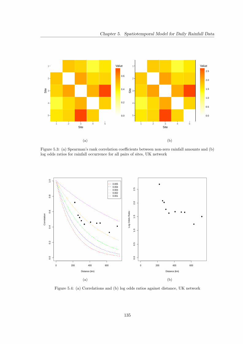
Chapter 5. Spatiotemporal Model for Daily Rainfall Data
1
2
3
4
5
1 2 3 4 5
Site
Site
0.0
0.2
0.4
0.6
Value
(a)
1
2
3
4
5
1 2 3 4 5
SiteS
ite
0.0
0.5
1.0
1.5
2.0
2.5
Value
(b)
Figure 5.3: (a) Spearman’s rank correlation coefficients between non-zero rainfall amounts and (b)log odds ratios for rainfall occurrence for all pairs of sites, UK network
0 200 400 600
0.0
0.2
0.4
0.6
0.8
1.0
Distance (km)
Co
rre
latio
n
0.0050.0040.0030.0020.001
(a)
0 200 400 600
0.0
0.5
1.0
1.5
2.0
2.5
Distance (km)
Lo
g O
dd
s R
atio
(b)
Figure 5.4: (a) Correlations and (b) log odds ratios against distance, UK network
135

Chapter 5. Spatiotemporal Model for Daily Rainfall Data
different values of the decay parameter, are also superimposed on Figure 5.4a. Apart fromone point, the point at the greatest distance, the fit to an exponential function with decayparameter around 0.002 seems reasonably good. There is no suggestion that the limit ofthe correlation as the distance tends to zero is less than 1 so there is no obvious need toinclude a “nugget” effect.
5.4 The model
5.4.1 Model structure
When building a spatiotemporal model for rainfall, it is natural to provide a more generalparameterisation for the model before we modify it to simplify the process. In our case,the daily rainfall patterns assume a mixed distribution. It is therefore crucial to considerthe relationship between the amount and occurrence processes. Following the discussionin Chapter 4, we opted for the same approach developed by Sofia (2007) whose conceptualframework relies on making the occurrence process dependent upon the amount process.Consequently, this method is contrary to the model implemented by Heaps et al. (2015)and Germain (2010). A similar parameterisation has been applied to a single site in NorthEast England. In this section, we will introduce and develop a spatiotemporal modelfor daily rainfall which is an extension of the previous univariate daily rainfall model inChapter 4, Section 4.4.
The resulting model structure is shown in the DAG in Figure 5.5. The structure isessentially the same as that for the univariate British rainfall model in Section 4.4 exceptthat now the nodes represent vector variables.
5.4.2 Modelling the rainfall amount
Following the univariate rainfall model elaborated in Chapter 4, Section 4.4, we will de-velop a spatiotemporal model for daily rainfall using the concept of the potential dailyrainfall amount. Firstly, the potential daily rainfall amount at site s on day t is assumedto follow a gamma distribution:
Yt(s)|xt = k, α, µt(s) ∼ Ga(α,
α
µt(s)
)(5.3)
136
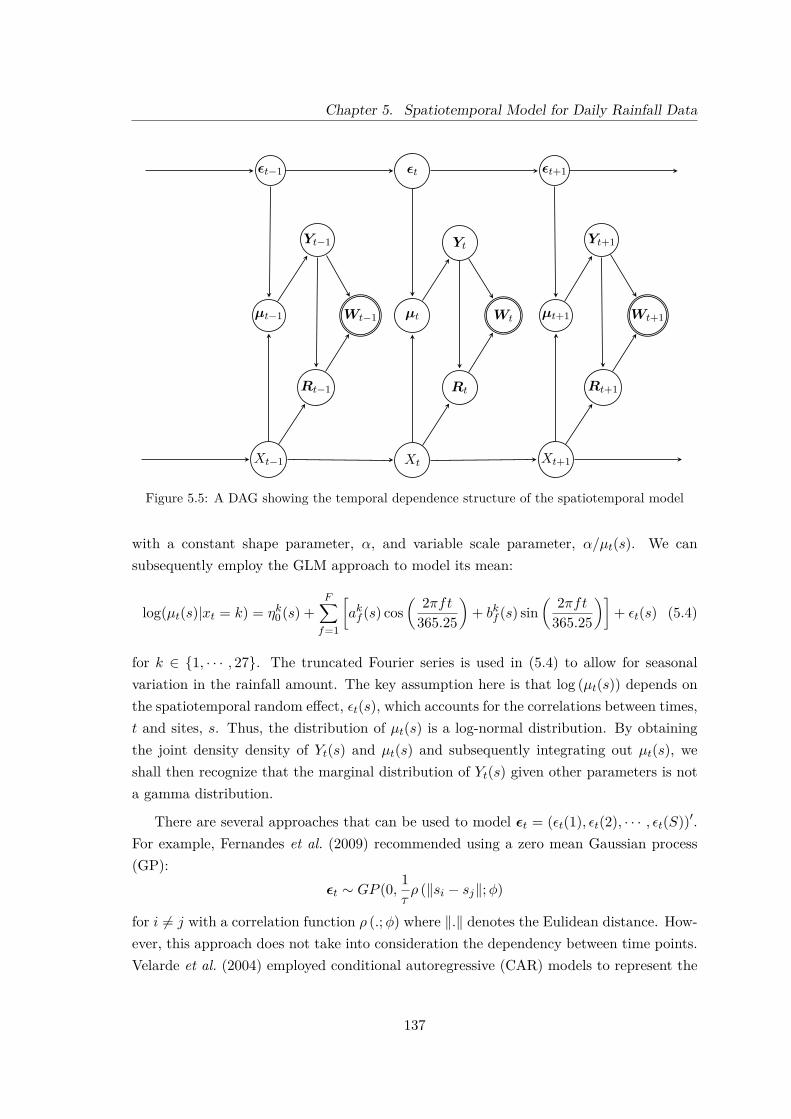
Chapter 5. Spatiotemporal Model for Daily Rainfall Data
εtεt−1 εt+1
µtµt−1 µt+1WtWt−1 Wt+1
YtYt−1 Yt+1
RtRt−1 Rt+1
XtXt−1 Xt+1
Figure 5.5: A DAG showing the temporal dependence structure of the spatiotemporal model
with a constant shape parameter, α, and variable scale parameter, α/µt(s). We cansubsequently employ the GLM approach to model its mean:
log(µt(s)|xt = k) = ηk0 (s) +F∑f=1
[akf (s) cos
( 2πft365.25
)+ bkf (s) sin
( 2πft365.25
)]+ εt(s) (5.4)
for k ∈ {1, · · · , 27}. The truncated Fourier series is used in (5.4) to allow for seasonalvariation in the rainfall amount. The key assumption here is that log (µt(s)) depends onthe spatiotemporal random effect, εt(s), which accounts for the correlations between times,t and sites, s. Thus, the distribution of µt(s) is a log-normal distribution. By obtainingthe joint density density of Yt(s) and µt(s) and subsequently integrating out µt(s), weshall then recognize that the marginal distribution of Yt(s) given other parameters is nota gamma distribution.
There are several approaches that can be used to model εt = (εt(1), εt(2), · · · , εt(S))′.For example, Fernandes et al. (2009) recommended using a zero mean Gaussian process(GP):
εt ∼ GP (0, 1τρ (‖si − sj‖;φ)
for i 6= j with a correlation function ρ (.;φ) where ‖.‖ denotes the Eulidean distance. How-ever, this approach does not take into consideration the dependency between time points.Velarde et al. (2004) employed conditional autoregressive (CAR) models to represent the
137

Chapter 5. Spatiotemporal Model for Daily Rainfall Data
spatiotemporal effects. This approach, introduced by Besag (1974), has been routinelyused for mapping disease (Waller & Carlin (2010), Reich et al. (2006), and Knorr-Held& Besag (1998)). In our model, we assume each εt is dependent on the previous value,εt−1, in a vector autoregression allowing for the temporal dependency. More specifically,suppose εt follows a multivariate normal distribution:
εt|εt−1 ∼ NS
(φεεt−1,
1τΣ
)(5.5)
for t > 1. For t = 1, the random effect is given by:
ε1 ∼ NS
(0, 1τ (1− φ2
ε )Σ
). (5.6)
The marginal mean of εt is zero with parameters φε and τ whereΣ is the spatial correlationmatrix. Banerjee et al. (2004) recommended some possible forms for the spatial covariancefunction and the most popular choice is the exponential covariance function which is givenby:
Σij = exp(−φ‖si − sj‖) (5.7)
with i 6= j, φ > 0 and ‖si − sj‖ is the distance between site si and sj . If i = j, the distanceis equal to zero. According to Sanso & Guenni (1999), this is the standard correlationfunction in hydrological applications which ensures that Σij is always symmetric andpositive definite. Another popular choice for the spatial covariance function is the Materncorrelation function which was originally introduced by Matern (1986).
This model also incorporates LWTs, xt, by applying them directly to the parameters ofthe linear function as shown in (5.4). This modelling strategy is in contrast to the methodsused by Heaps et al. (2015) and Germain (2010) who introduced the LWTs through thehidden Markov models. Since many parameters are dependent on the LWTs and site, thereis a strong possibility of poor identification of some parameters. Therefore, we simplifythe parameterisation in (5.4) by allowing only ηk0 (s) to depend on the LWTs while theFourier coefficients are constant over LWTs and sites. Thus, the new parameterisation forlog (µt(s)) is :
log(µt(s)|xt = k) = ηk0 (s) +F∑f=1
[af cos
( 2πft365.25
)+ bf sin
( 2πft365.25
)]+ εt(s).
138

Chapter 5. Spatiotemporal Model for Daily Rainfall Data
5.4.3 Modelling the rainfall occurrence
The rainfall occurrence can only take the values of either 0 or 1, therefore the appropriateprobability mass function (pmf) for the occurrence process is a Bernoulli distribution:
Rt(s)|xt = k, yt(s) ∼ Bern (p1(s, t)) (5.8)
where p1(s, t) is the rainfall probability at site s on day t. There are several approachesthat we can use to model the probability of rainfall which have already been discussedin Chapter 4, Section 4.2.3. The most common approach is a logit link function. Analternative approach is a probit link function which has been used by Heaps et al. (2015),Germain (2010) and Thompson et al. (2007). We then propose to apply a logit linkfunction in this occurrence process to model the rainfall probability as follows:
logit(p1(s, t)|xt = k
)=ζk0 (s) +
F∑f=1
[ckf (s) cos
( 2πft365.25
)+ dkf (s) sin
( 2πft365.25
)]+ ζk1 (s) log
(yt(s)
) (5.9)
for k ∈ {1, · · · , 27}. Similar to the amount process, the truncated Fourier series is used toallow for seasonal variation in the rainfall probability. Note that logit
(p1(s, t)|xt = k
)is
conditioned upon log (yt(s)) to create a link between the amount and occurrence processes.This parameterisation is in contrast to that of Heaps et al. (2015) and Germain (2010)who used the rainfall occurrence as a covariate to construct a model for the log-rainfallamounts. We do not include the spatiotemporal effect directly in the occurrence processsince the spatiotemporal effect has already been represented by yt(s).
Similar to the amount process, the original idea is to apply the LWTs directly to allparameters in the logit function (5.9). However, this may lead to poor identification ofsome parameters. Therefore, we simplify the parameterisation by applying the LWTs onlyto ζk0 (s) while the Fourier coefficients and ζ1 are constant over LWTs and sites. Thus, thenew parameterisation for the occurrence process is
logit(p1(s, t)|xt = k
)= ζk0 (s) +
F∑f=1
[cf cos
( 2πft365.25
)+ df sin
( 2πft365.25
)]+ ζ1 log
(yt(s)
).
139

Chapter 5. Spatiotemporal Model for Daily Rainfall Data
5.5 Prior distribution
5.5.1 Prior distribution for the amount process
Since the shape parameter, α can only take positive values, it is assigned a gamma distri-bution:
α ∼ Ga(gα, hα).
For the intercept term, ηk0 (s), we assign a common prior mean, mη0, for all s and k. Inorder to generate an appropriate prior covariance structure for the collection of interceptterms, we represent the deviations from the prior mean in terms of a number of zero-meanrandom variables, η01(k), η0,2(s) and η0,3(k, s), which are mutually independent, in thestyle of Farrow (2003). Thus we write
ηk0 (s) = mη0 + η01(k) + η0,2(s) + η0,3(k, s).
In the cases of η01(k) and η0,2(s), we introduce hierarchical structures. By conditioningη01(k) on η01, we have
η01(k) | η01 ∼ N(η01, vη1)
whereη01 ∼ N(0, vη0)
and the variance, covariance and correlation are given by:
Var[η01(k)] = vη0 + vη1 ,
Covar[η01(k), η0,1(k′)] = vη0 ,
Corr[η01(k), η0,1(k′)] = vη0
vη0 + vη1.
Similarly, for η02(s), we have
η02(s) | η02 ∼ N(η02, vη1)
whereη02 ∼ N(0, vη0)
140

Chapter 5. Spatiotemporal Model for Daily Rainfall Data
and
Var[η02(s)] = vη0 + vη1 ,
Covar[η02(s), η0,2(s)] = vη0 ,
Corr[η02(s), η0,2(s)] = vη0
vη0 + vη1.
The terms η0,3(k, s) are mutually independent and
η03(k, s) ∼ N(0, τ−1η3 ).
In the terminology of Farrow (2003), η01(k) and η02(s) are common uncertainty factorsand the terms η03(k, s) are specific uncertainty factors.
Let η = (a1, a2, b1, b2)′ represent the collection of Fourier coefficients for the amountprocess. Then, the prior distribution for η is given by:
η ∼ N4(mη, P
−1η
)where mη is the mean vector with precision matrix, Pη. For the parameters τ and φ,gamma distributions are assigned as their priors:
τ ∼ Ga(gτ , hτ )
andφ ∼ Ga(gφ, hφ).
A gamma distribution is a sensible prior choice for τ and φ since it can only assume positivevalues. The prior distribution for φε must adhere to the stationary condition |φε| < 1.Suppose that a new variable, v, follows a beta distribution:
v ∼ Beta(av, bv).
Since the beta distribution has a range between 0 and 1, we can then fix:
φε = 2v − 1
so that the value for φε is between -1 and 1.
141

Chapter 5. Spatiotemporal Model for Daily Rainfall Data
5.5.2 Prior distribution for the occurrence process
The prior distribution for the parameters in the occurrence process is similar to that forthe amount process. Let the intercept term ζk0 (s) is given by:
ζk0 (s) = mζ0 + ζ01(k) + ζ02(s) + ζ03(k, s)
where mζ0 is a common prior mean for all s and k. Similar to the amount process, ζ01(k),ζ02(s) and ζ03(k, s) are given to generate an approriate prior covariance structure for thecollection of intercept terms.
In the case of ζ01(k) and ζ02(s), we introduce hierarchical structures. By conditioningζ01(k) upon ζ01, the distribution of ζ01(k) is:
ζ01(k)|ζ01 ∼ N(ζ01, υζ1)
whereζ01 ∼ N(0, υζ0)
and the variance, covariance and correlation are given by:
Var[ζ01(k)] =υζ0 + υζ1
Covar[ζ01(k), ζ01(k′)] =υζ0
Corr[ζ01(k), ζ01(k′)] = υζ0
υζ0 + υζ1
.
Similarly, for ζ02(s), we have:
ζ02(s)|ζ02 ∼ N(ζ02, νζ1)
whereζ02 ∼ N(0, νζ0)
and
Var[ζ02(s)] =νζ0 + νζ1
Covar[ζ02(s), ζ02(s′)] =νζ0
Corr[ζ02(s), ζ02(s′)] = νζ0
νζ0 + νζ1
.
The terms ζ03(k, s) are mutually independent and:
ζ03(k, s) ∼ N(0, 1/τ−1
ζ3
).
142

Chapter 5. Spatiotemporal Model for Daily Rainfall Data
By following the terminology of Farrow (2003), ζ01(k) and ζ02(s) are common uncertaintyfactors and the terms ζ03(k, s) are specific uncertainty factors. A normally-distributedprior is also assigned for ζ1:
ζ1 ∼ N (mζ1 , 1/τζ1)
since ζ1 can take any values from −∞ to ∞.
Let the set of Fourier coefficients for the occurrence process be represented by ζ =(c1, c2, d1, d2)′. Then, the prior distribution for the Fourier coefficients is defined in asimilar manner as for the amount process:
ζ ∼ N4(mζ , P
−1ζ
)where mζ and Pζ are the mean vector and the precision matrix, respectively.
5.6 Posterior distribution
Let θ be the collection of unknown parameters. The joint density of (θ,Y ,R) is thengiven by:
π(θ,y, r) = π(θamt)× π(θocc)× f(y|θamt)× f(r|y,θocc) (5.10)
where θamt and θocc are the collections of parameters for the amount and occurrenceprocesses, respectively. To evaluate the posterior distribution, we use a Metropolis-within-Gibbs algorithm. We use data augmentation and treat the unobserved potential rainfallamounts Yt(s) and the random effects εt(s) as auxiliary data. We therefore need to findthe full conditional distributions of the model parameters and the auxiliary data.
5.6.1 The full conditional distributions for the amount process
From (5.10), we can work out the full conditional distribution (FCD) for each parameterin the amount process. The FCDs in this section are provided only as general informationand for future work. Then, the FCD for each parameter are derived as follows:
143
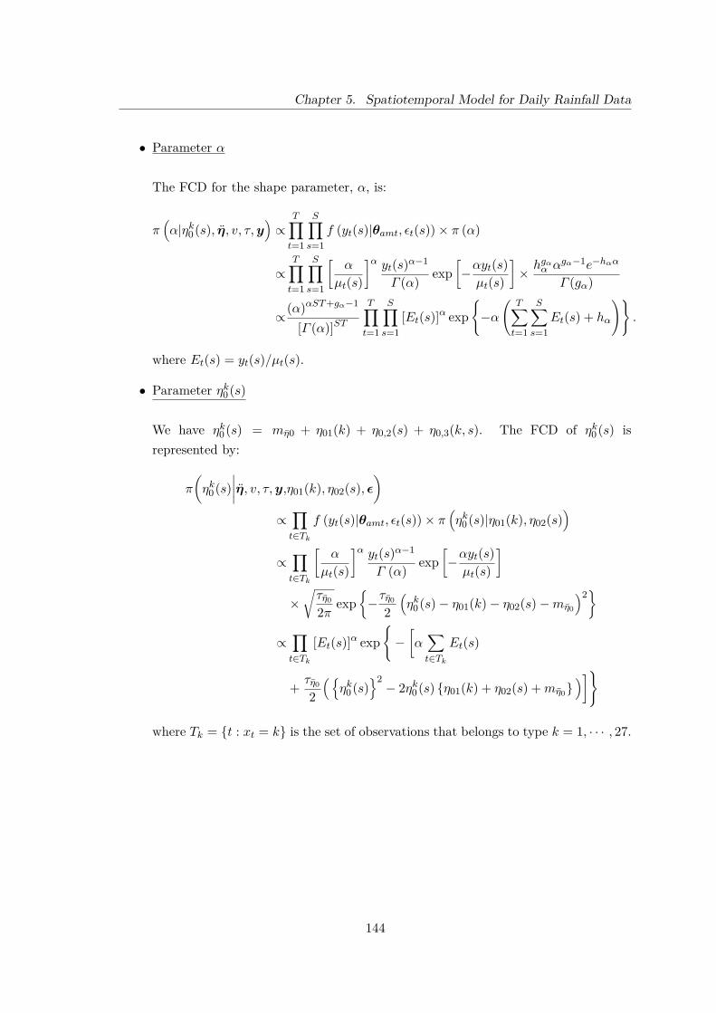
Chapter 5. Spatiotemporal Model for Daily Rainfall Data
• Parameter α
The FCD for the shape parameter, α, is:
π(α|ηk0 (s), η, v, τ,y
)∝
T∏t=1
S∏s=1
f (yt(s)|θamt, εt(s))× π (α)
∝T∏t=1
S∏s=1
[α
µt(s)
]α yt(s)α−1
Γ (α) exp[−αyt(s)µt(s)
]× hgαα α
gα−1e−hαα
Γ (gα)
∝(α)αST+gα−1
[Γ (α)]STT∏t=1
S∏s=1
[Et(s)]α exp{−α
(T∑t=1
S∑s=1
Et(s) + hα
)}.
where Et(s) = yt(s)/µt(s).
• Parameter ηk0 (s)
We have ηk0 (s) = mη0 + η01(k) + η0,2(s) + η0,3(k, s). The FCD of ηk0 (s) isrepresented by:
π
(ηk0 (s)
∣∣∣∣η, v, τ,y,η01(k), η02(s), ε)
∝∏t∈Tk
f (yt(s)|θamt, εt(s))× π(ηk0 (s)|η01(k), η02(s)
)
∝∏t∈Tk
[α
µt(s)
]α yt(s)α−1
Γ (α) exp[−αyt(s)µt(s)
]
×√τη0
2π exp{−τη0
2(ηk0 (s)− η01(k)− η02(s)−mη0
)2}
∝∏t∈Tk
[Et(s)]α exp{−[α∑t∈Tk
Et(s)
+ τη0
2({
ηk0 (s)}2− 2ηk0 (s) {η01(k) + η02(s) +mη0}
)]}
where Tk = {t : xt = k} is the set of observations that belongs to type k = 1, · · · , 27.
144

Chapter 5. Spatiotemporal Model for Daily Rainfall Data
The FCD of η01(k) is given by:
π
(η01(k)
∣∣∣∣ηk0 (1), · · · , ηk0 (S),η02(1), · · · , η02(S), η01
)
∝S∏s=1
f(ηk0 (s)|η01(k), η02(s)
)× π (η01(k)|η01)
∝S∏s=1
√τη0
2π exp{−τη0
2(ηk0 (s)− η01(k)− η02(s)−mη0
)2}
×√
12πυη1
exp{− 1
2υη1(η01(k)− η01)2
}
∝ exp{−Dη01
2 (η01(k)−Bη01)2}
whereDη01 = Sτη0 + 1
υη1
and
Bη01 = 1Dη01
{τη0
[S∑s=1
ηk0 (s)−S∑s=1
η02(s)− Smη0
]+ η01υη1
}.
This form corresponds to a normal density, N(Bη01 , 1/Dη01).
The FCD of η01 is derived as follows:
π
(η01
∣∣∣∣η01(1), · · · , η01(27))∝
27∏k=1
f (η01(k)|η01)× π(η01)
∝27∏k=1
√1
2πυη1exp
{− 1
2υη1(η01(k)− η01)2
}
×√
12πυη0
exp{− 1
2υη0(η01)2
}
∝ exp{Dη01
2(η01 − Bη01
)2}
whereDη01 = K
υη1+ 1υη0
andBη01 =
∑27k=1 η01(k)Dη01υη0
.
This form also corresponds to a normal density, N(Bη01 , 1/Dη01).
145

Chapter 5. Spatiotemporal Model for Daily Rainfall Data
The FCD of η02(s) is represented by:
π
(η02(s)
∣∣∣∣η10(s), · · · , η27
0 (s),η01(1), · · · , η01(27), η02
)
∝27∏k=1
f(ηk0 (s)|η01(k), η02(s)
)× π (η02(s)|η02)
∝27∏k=1
√τη0
2π exp{−τη0
2(ηk0 (s)− η01(k)− η02(s)−mη0
)2}
×√
12πνη1
exp{− 1
2νη1(η02(s)− η02)2
}
∝ exp{−Dη02
2 (η02(s)−Bη02)2}
whereDη02 = Sτη0 + 1
νη1
and
Bη02 = 1Dη02
{τη0
[ 27∑k=1
ηk0 (s)−27∑k=1
η01(k)−Kmη0
]+ η02νη1
}.
This is a normal distribution.
For η02, the FCD is:
π
(η02
∣∣∣∣η02(1), · · · , η02(S))∝
S∏s=1
f (η02(s)|η02)× π(η02)
∝S∏s=1
√1
2πνη1exp
{− 1
2νη1(η02(s)− η02)2
}
×√
12πνη0
exp{− 1
2νη0η02
}
∝ exp{Dη02
2(η01 − Bη02
)2}
whereDη02 = S
νη1+ 1νη0
andBη02 =
∑Ss=1 η02(s)Dηνη0
.
Again, this is the density form of a normal distribution.
146

Chapter 5. Spatiotemporal Model for Daily Rainfall Data
• Parameter η
The FCD for η is given by:
π(η|ηk0 (s), v, τ,y
)∝
T∏t=1
S∏s=1
f (yt(s)|θamt, εt(s))× π (η)
∝T∏t=1
S∏s=1
[α
µt(s)
]α yt(s)α−1
Γ (α) exp[−αyt(s)µt(s)
]× (2π)−2F |Pη|1/2 exp
{−1
2(η −mη)TPη(η −mη)}
∝T∏t=1
S∏s=1
[Et(s)]α exp{−[α
T∑t=1
S∑s=1
Et(s) + 12(η −mη)TPη(η −mη)
]}.
• Parameter v
The FCD for v can be derived as follows:
π (v|ε, φ, τ) ∝f (ε1|v, φ, τ)T∏t=2
f (εt|εt−1, v, φ, τ)× π (v)
∝√τ (1− φ2
ε )(2π)S |Σ| exp
{−τ
(1− φ2
ε
)2 (ε1)′Σ−1 (ε1)
}
×T∏t=2
√τ
(2π)S |Σ| exp{− τ
2(εt − φεεt−1
)′Σ−1(εt − φεεt−1
)}
× Γ (av + bv)Γ (av)Γ (bv)
vav−1(1− v)bv−1
∝vav−1(1− v)bv−1√
(1− φ2ε ) exp
{− τ
2
[(1− φ2
ε
)(ε1)′Σ−1 (ε1)
+T∑t=1
(εt − φεεt−1)′Σ−1(εt − φεεt−1)]}.
147

Chapter 5. Spatiotemporal Model for Daily Rainfall Data
• Parameter φ
For φ, the FCD can be expressed using the following:
π (φ|ε, v, τ) ∝f (ε1|v, φ, τ)T∏t=2
f (εt|εt−1, v, φ, τ)× π (φ)
∝√τ (1− φ2
ε )(2π)S |Σ| exp
{−τ
(1− φ2
ε
)2 (ε1)′Σ−1 (ε1)
}
×T∏t=2
√τ
(2π)S |Σ| exp{− τ
2(εt − φεεt−1
)′Σ−1(εt − φεεt−1
)}
×hgφφ φ
gφ−1 exp [−hφφ]Γ (gφ)
∝φgφ−1 exp{−[τ
2[(
1− φ2ε
)(ε1)′Σ−1 (ε1) +
T∑t=2
(εt − φεεt−1
)′Σ−1(εt − φεεt−1
)]+ hφφ
]}.
• Parameter τ
The full conditional distribution for τ is:
π (τ |ε, v, φ) ∝f (ε1|v, φ, τ)T∏t=2
f (εt|εt−1, v, φ, τ)× π (τ)
∝√τ (1− φ2
ε )(2π)S |Σ| exp
{−τ
(1− φ2
ε
)2 (ε1)′Σ−1 (ε1)
}
×T∏t=2
√τ
(2π)S |Σ| exp{− τ
2(εt − φεεt−1
)′Σ−1(εt − φεεt−1
)}
× hgττ τgτ−1 exp [−hττ ]Γ (gτ )
∝τ gτ+T2 −1
{− τ
[12(1− φ2
ε
)(ε1)′Σ−1 (ε1)
+ 12
T∑t=1
(εt − φεεt−1)′Σ−1(εt − φεεt−1) + hτ
]}.
This form corresponds to a gamma density, Ga(Gτ , Hτ ) where
Gτ = gτ + T
2
148

Chapter 5. Spatiotemporal Model for Daily Rainfall Data
and
Hτ =[1
2(1− φ2
ε
)(ε1)′Σ−1 (ε1) + 1
2
T∑t=1
(εt − φεεt−1)′Σ−1(εt − φεεt−1) + hτ
].
• Random effect εt
To obtain the sampled values for the random effect εt, the FCD for εt isworked out as follows:
π (εt|φε, φ, τ,yt) ∝S∏s=1
f (yt(s)|θamt, εt)× π (εt|εt−1)× π (εt+1|εt)
∝S∏s=1
[α
µt(s)
]α yt(s)α−1
Γ (α) exp[−αyt(s)µt(s)
]
×√
τ
(2π)S |Σ| exp{− τ
2(εt − φεεt−1
)′Σ−1(εt − φεεt−1
)}
×√
τ
(2π)S |Σ| exp{− τ
2(εt+1 − φεεt
)′Σ−1(εt+1 − φεεt
)}
∝S∏s=1
[Et(s)]α exp{−[α
S∑s=1
Et(s) + τ
2[Qt +Qt+1
]]}
whereQt = (εt − φεεt−1)′Σ−1 (εt − φεεt−1)
for 1 < t < T − 1. For t = 1, the FCD is given by:
π (ε1|φε, φ, τ,y1) ∝S∏s=1
f (y1(s)|θamt, ε1)× π (ε1)× π (ε2|ε1)
∝S∏s=1
[α
µ1(s)
]α y1(s)α−1
Γ (α) exp[−αy1(s)µ1(s)
]
×√τ (1− φ2
ε )(2π)S |Σ| exp
{−τ
(1− φ2
ε
)2 (ε1)′Σ−1 (ε1)
}
×√
τ
(2π)S |Σ| exp{− τ
2(ε2 − φεε1
)′Σ−1(ε2 − φεε1
)}
∝S∏s=1
[E1(s)]α exp{−[α
S∑s=1
E1(s) + τ
2[ (
1− φ2ε
)(ε1)′Σ−1 (ε1)
+ (ε2 − φεε1)′Σ−1 (ε2 − φεε1)]]}
149

Chapter 5. Spatiotemporal Model for Daily Rainfall Data
and the FCD for εT is
π (εT |φε, φ, τ,yT ) ∝S∏s=1
f (yT (s)|θamt, εT )× π (εT |εT−1)
∝S∏s=1
[α
µT (s)
]α yT (s)α−1
Γ (α) exp[−αyT (s)µT (s)
]
×√
τ
(2π)S |Σ| exp{− τ
2(εT − φεεT−1
)′Σ−1(εT − φεεT−1
)}
∝S∏s=1
[ET (s)]α exp{−[α
S∑s=1
ET (s) + τ
2QT]}
whereQT = (εT − φεεT−1)′Σ−1 (εT − φεεT−1) .
• Latent y-values: ydry
When Wt(s) = 0, the latent value, yt(s), is not observed and we can henceregard it as ydry. In this case, the values of ydry are treated as auxiliary data withinthe data augmentation framework. Therefore, the FCD for ydry can be written as:
π(ydry|rt(s) = 0, α, µt(s)) ∝f(ydry|α, µt(s))× Pr(Rt(s) = 0|ydry,θocc)
∝(α/µt(s))αyα−1
dry e−(α/µt(s))ydry
Γ (α) × p0(s, t)
for every rt(s) = 0 where p0(t, s) = 1− p1(t, s) is the probability of a dry day whichdepends on yt(s).
The FCDs of the majority of parameters in the amount process are not in standard forms.Therefore, we have to utilise a Metropolis-within-Gibbs scheme to obtain the posteriorsamples for each parameter.
5.6.2 Full conditional distributions for the occurrence process
Suppose that we want to obtain posterior samples for each parameter in the occurrenceprocess. Therefore, we need to derive the FCD for each parameter from equation (5.10).Similar to the amount process, the FCDs are provided as general information and forfuture work. The FCD for each parameter is given as follows:
150
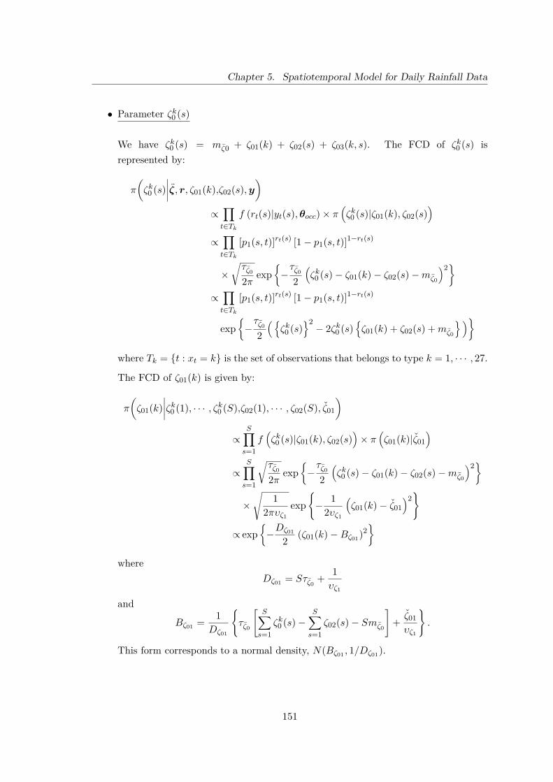
Chapter 5. Spatiotemporal Model for Daily Rainfall Data
• Parameter ζk0 (s)
We have ζk0 (s) = mζ0 + ζ01(k) + ζ02(s) + ζ03(k, s). The FCD of ζk0 (s) isrepresented by:
π
(ζk0 (s)
∣∣∣∣ζ, r, ζ01(k),ζ02(s),y)
∝∏t∈Tk
f (rt(s)|yt(s),θocc)× π(ζk0 (s)|ζ01(k), ζ02(s)
)∝∏t∈Tk
[p1(s, t)]rt(s) [1− p1(s, t)]1−rt(s)
×√τζ0
2π exp{−τζ0
2(ζk0 (s)− ζ01(k)− ζ02(s)−mζ0
)2}
∝∏t∈Tk
[p1(s, t)]rt(s) [1− p1(s, t)]1−rt(s)
exp{−τζ0
2({
ζk0 (s)}2− 2ζk0 (s)
{ζ01(k) + ζ02(s) +mζ0
})}where Tk = {t : xt = k} is the set of observations that belongs to type k = 1, · · · , 27.
The FCD of ζ01(k) is given by:
π
(ζ01(k)
∣∣∣∣ζk0 (1), · · · , ζk0 (S),ζ02(1), · · · , ζ02(S), ζ01
)
∝S∏s=1
f(ζk0 (s)|ζ01(k), ζ02(s)
)× π
(ζ01(k)|ζ01
)
∝S∏s=1
√τζ0
2π exp{−τζ0
2(ζk0 (s)− ζ01(k)− ζ02(s)−mζ0
)2}
×√
12πυζ1
exp{− 1
2υζ1
(ζ01(k)− ζ01
)2}
∝ exp{−Dζ01
2 (ζ01(k)−Bζ01)2}
whereDζ01 = Sτζ0
+ 1υζ1
and
Bζ01 = 1Dζ01
{τζ0
[S∑s=1
ζk0 (s)−S∑s=1
ζ02(s)− Smζ0
]+ ζ01υζ1
}.
This form corresponds to a normal density, N(Bζ01 , 1/Dζ01).
151
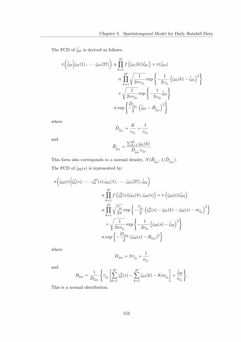
Chapter 5. Spatiotemporal Model for Daily Rainfall Data
The FCD of ζ01 is derived as follows:
π
(ζ01
∣∣∣∣ζ01(1), · · · , ζ01(27))∝
27∏k=1
f(ζ01(k)|ζ01
)× π(ζ01)
∝27∏k=1
√1
2πυζ1
exp{− 1
2υζ1
(ζ01(k)− ζ01
)2}
×√
12πυζ0
exp{− 1
2υζ0
ζ01
}
∝ exp{Dζ01
2(ζ01 − Bζ01
)2}
whereDζ01
= K
υζ1
+ 1υζ0
andBζ01
=∑27k=1 ζ01(k)Dζ01
υζ0
.
This form also corresponds to a normal density, N(Bζ01, 1/Dζ01
).
The FCD of ζ02(s) is represented by:
π
(ζ02(s)
∣∣∣∣ζ10 (s), · · · , ζ27
0 (s),ζ01(1), · · · , ζ01(27), ζ02
)
∝27∏k=1
f(ζk0 (s)|ζ01(k), ζ02(s)
)× π
(ζ02(s)|ζ02
)
∝27∏k=1
√τζ0
2π exp{−τζ0
2(ζk0 (s)− ζ01(k)− ζ02(s)−mζ0
)2}
×√
12πνζ1
exp{− 1
2νζ1
(ζ02(s)− ζ02
)2}
∝ exp{−Dζ02
2 (ζ02(s)−Bζ02)2}
whereDζ02 = Sτζ0
+ 1νζ1
and
Bζ02 = 1Dζ02
{τζ0
[ 27∑k=1
ζk0 (s)−27∑k=1
ζ01(k)−Kmζ0
]+ ζ02νζ1
}.
This is a normal distribution.
152
Chapter 5. Spatiotemporal Model for Daily Rainfall Data
For ζ02, the FCD is:
π
(ζ02
∣∣∣∣ζ02(1), · · · , ζ02(S))∝
S∏s=1
f(ζ02(s)|ζ02
)× π(ζ02)
∝S∏s=1
√1
2πνζ1
exp{− 1
2νζ1
(ζ02(s)− ζ02
)2}
×√
12πνζ0
exp{− 1
2νζ0
(ζ02)2}
∝ exp{Dζ02
2(ζ01 − Bζ02
)2}
whereDζ02
= S
νζ1
+ 1νζ0
andBζ02
=∑Ss=1 ζ02(s)Dζνζ0
.
Again, this is the density form of a normal distribution.
• Parameter ζ
The FCD for ζ can be derived as follows:
π(ζ|ζk0 (s), ζ1, r,y
)∝
T∏t=1
S∏s=1
f (rt(s)|yt(s),θocc)× π(ζ)
∝T∏t=1
S∏s=1
[p1(s, t)]rt(s) [1− p1(s, t)]1−rt(s)
× (2π)−4|Pζ |1/2 exp
{−1
2(ζ −mζ)′Pζ(ζ −mζ)
}
∝T∏t=1
S∏s=1
[p1(s, t)]rt(s) [1− p1(s, t)]1−rt(s)
exp{−1
2(ζ −mζ)′Pζ(ζ −mζ)
}.
153
Chapter 5. Spatiotemporal Model for Daily Rainfall Data
• Parameter ζ1(s)
For ζ1, the FCD is given by:
π(ζ1|ζk0 (s), ζ, r,y
)∝
T∏t=1
S∏s=1
f (rt(s)|yt(s),θocc)× π (ζ1)
∝T∏t=1
S∏s=1
[p1(s, t)]rt(s) [1− p1(s, t)]1−rt(s)
×√τζ1
2π exp{−τζ1
2 (ζ1 −mζ1)2}
∝T∏t=1
S∏s=1
[p1(s, t)]rt(s) [1− p1(s, t)]1−rt(s)
exp{−τζ1
2(ζ2
1 − 2ζ1mζ1
)}.
Similar to the amount process, the FCDs of the majority of parameters for the occurrenceprocess are not of any standard form. Therefore, we require a Metropolis-within-Gibbsscheme to sample the posterior values for each parameter.
5.7 Application
5.7.1 Prior distributions
Similar to the previous models, the prior distributions for the spatiotemporal model wereelicited using the information gained from previous studies and personal beliefs. The priorconstruction for a single site in the UK has already been discussed in Chapter 4, Section4.4.5.1. Therefore, we will use the same argument for the spatiotemporal model to specifythe priors since the sites are within the same network.
For the additional parameter φ, which governs the spatial correlation, we follow theidea of Banerjee et al. (2004) by considering the “effective range” D as follows:
e−φD =0.05
so − φD = log(0.05)
so φ =− log(0.05)D
where D is the interlocation distance at which the between-site correlation has fallen to0.05. We can use a direct approach to elicit prior quartiles for D and then convert these toprior quartiles for φ. Let our prior quartiles for φ be Qφ,1, Qφ,2 and Qφ,3, respectively. We
154

Chapter 5. Spatiotemporal Model for Daily Rainfall Data
give φ a Ga(gφ, hφ) distribution. Since hφ is a scale parameter, Qφ,3/Qφ,1 depends only ongφ where gφ can be determined using numerical iteration to solve Qφ,3/Qφ,1 = R3(a)/R1(a)where Rq(a) is quartile q for a Ga(a, 1) distribution. Once gφ is obtained, then we can findthe value for hφ using R2(gφ)/Qφ,2. Suppose that the prior median for the effective rangeis 750 km, then the prior median of φ is Qφ,2 = 0.004. We have also chosen carefully asuitable value of the lower and upper quartiles for illustration where we have Qφ,1 = 0.001and Qφ,3 = 0.0045, respectively. Using this method, we have gφ = 1.07 and hφ = 190.59.
In this spatiotemporal model, we employed a Fourier series with just two harmonicsfor the amount process. The prior elicitation for the Fourier coefficients is still the same asin Section 4.3.3.3. The full prior specifications for the unknown parameters of the amountprocess can be summarised as follows:
α ∼ Ga(4.31, 5.78); v ∼ Beta(3.7, 1.9);
τ ∼ Ga(3.69, 1.69); φ ∼ N(1.07, 190.59);
andη ∼ N4
(η0, P
−1η
)where
η0 =
0000
, P−1η =
2π 0 0 00 1
π 0 00 0 2
π 00 0 0 1
π
for k ∈ {1, · · · , 27} and s ∈ {1, · · · , 5}.
Based on the previous univariate British model, we have chosen the prior mean of η0
to be 0.69. Then, we will use the same argument to give a value for mη0. In the caseof η01(k), η02(s) and η03(k, s), we have chosen a suitable values for the variances of theuncertainty factors as follows:
η01(k)|η01 ∼ N(η01, 1); η01 ∼ N(0, 1)
η02(s)|η02 ∼ N(η02, 1); η02 ∼ N(0, 1)
η03(k, s) ∼ N(0, 4).
This gives ηk0 (s) a marginal prior variance of 8. Let k′ 6= k and s′ 6= s. The covariancebetween ηk0 (s) and ηk
′0 (s) is 3, giving a correlation 0f 0.375. Similarly the covariance
between ηk0 (s) and ηk0 (s′) is 3, giving a correlation 0f 0.375. The covariance between ηk0 (s)and ηk
′0 (s′) is 2, giving a correlation of 0.250. Thus the prior correlations are fairly weak.
For the occurrence process, we also use the same argument as for the British univariate
155

Chapter 5. Spatiotemporal Model for Daily Rainfall Data
model and the amount process to elicit the prior for the unknown parameters. We willuse two harmonics of the Fourier series to represent the seasonal effect of the rainfalloccurrence over the year. Hence, the prior specifications for the unknown parameters forthe occurrence process are given by the following:
ζ1 ∼ N(1.29, 3.12)
andζ ∼ N4
(ζ0, P
−1ζ
)where
ζ0 =
0000
, P−1ζ
=
2π 0 0 00 1
π 0 00 0 2
π 00 0 0 1
π
for k ∈ {1, · · · , 27} and s ∈ {1, · · · , 5}.
The values for mζ0 and the variances of ζ01(k), ζ02(s) and ζ03(k, s) are chosen as follows:
ζ01(k)|ζ01 ∼ N(ζ01, 1); ζ01 ∼ N(0, 1)
ζ02(s)|ζ02 ∼ N(ζ02, 1); ζ02 ∼ N(0, 1)
ζ03(k, s) ∼ N(0, 5.52); mζ0 = 1.03.
This gives ζk0 (s) a marginal prior variance of 9.52. Let k′ 6= k and s′ 6= s. Thecovariance between ζk0 (s) and ζk
′0 (s) is 3, giving a correlation 0f 0.315. Similarly the
covariance between ζk0 (s) and ζk0 (s′) is 3, giving a correlation 0f 0.315. The covariancebetween ζk0 (s) and ζk
′0 (s′) is 2, giving a correlation of 0.210. Thus the prior correlations
are again fairly weak.
5.7.2 Fitting the model
The Rjags package (Plummer, 2012) is used to compute the posterior samples for thismodel. The MCMC algorithm was run for 50000 iterations to allow for burn-in, and anadditional 150000 iterations were drawn as the posterior samples. The computing timethat was required to generate 150000 posterior draws was around 240 hours by usingR software on a 2.00GHz Samsung laptop 300V3A model with Intel Core i7-2630QMprocessor and 12 Gbytes of random-access memory. The trace plots can be used as avisual diagnostic method to monitor the convergence of the sampler. Before we makeany inferences or conclusions, it is essential to look at the trace plots for parameters.
156

Chapter 5. Spatiotemporal Model for Daily Rainfall Data
Figure 5.6 displays the example of trace plots and posterior densities for α, τ and ζ1.Based on the trace plots, the mixing appears very satisfactory for the majority of theunknown parameters. However, some of the unknown parameters have a relatively highautocorrelation, which suggests mixing is a little slower. This can be seen in Figure5.6 for the parameters α and τ which suggest that the effective sample size (ESS) of theparameters is likely to be extremely low. The ESS is the number of effectively independentsamples obtained from the posterior distribution. The issue of low posterior sample sizefor α and τ happens because both α and τ contribute to the variance of the rainfallamount and therefore they are, to some extent, confounded. As a result, they are stronglynegatively correlated in the posterior. This might also suggest that a large number ofiterations are required to obtain a good representation of the posterior distribution.
The uncertainty associated with most of the unknown parameters has been reducedafter we combined the prior beliefs with the data. For example, there is a reduction in thevariability of parameter ζ1 when a comparison is made between the prior and posteriordistributions. The posterior mean of parameter ζ1 is shifted to the right of its prior mean.The full summaries of posterior means and standard deviations of the unknown parametersfor the amount and occurrence processes at Balmoral weather station are given in Tables5.2 and 5.3 (see Appendices A.1 and A.2 for the other weather stations).
In this spatiotemporal model, it is also important to observe the parameter φ sinceit controls the rate of decay of the correlation as the distance between sites increases.From Table 5.2, we can observe that the posterior value for φ is centred around 0.0012.This suggests that the correlation falls to 0.5 after about 578 km. This implies highspatial correlation even at large distances. Figure 5.4 suggests that the correlation doesnot decrease quickly with increasing distance. It may also be that the correlation doesnot tend to 1 as the distance tends to zero because of a “nugget effect”. For this reason,it might be better to use a different spatial correlation function. A lot of the correlationmay be explained by the LWT, leaving little for the spatial effect to explain. The LWTplays an important role in determining the rainfall amount and probability at time t. Thisis supported by looking at Figures 5.7 and 5.8. These plots show the posterior meansand 95% credible intervals of the intercepts parameters ηk0 (s) and ζk0 (s) for all weatherstations. It can be seen that the value for the LWT of type 1 (Anticylconic) is quite smallfor both processes despite being the most commonly-occurred LWT. The previous randomeffect at time t − 1 also plays a crucial role in determining the level of rainfall at time t.It is therefore highly possible that the rainfall amount will increase if rainfall did occur onthe previous day.
For model checking, we chose two weather stations that have the maximum and min-imum mean of daily rainfall amounts and these are Bastreet and Ardleigh Hull Farm
157

Chapter 5. Spatiotemporal Model for Daily Rainfall Data
Amount processParameter Prior mean Prior SD Posterior mean Posterior SDα 0.75 0.36 1.153 0.037η1
0(1) 0.69 2.83 -0.927 0.075η2
0(1) 0.69 2.83 -0.194 0.267η3
0(1) 0.69 2.83 -0.389 0.298η4
0(1) 0.69 2.83 -1.065 0.289η5
0(1) 0.69 2.83 -1.523 0.239η6
0(1) 0.69 2.83 -1.256 0.167η7
0(1) 0.69 2.83 -0.656 0.140η8
0(1) 0.69 2.83 0.183 0.161η9
0(1) 0.69 2.83 0.645 0.190η10
0 (1) 0.69 2.83 0.266 0.190η11
0 (1) 0.69 2.83 -0.048 0.203η12
0 (1) 0.69 2.83 -0.647 0.168η13
0 (1) 0.69 2.83 -1.184 0.122η14
0 (1) 0.69 2.83 -0.468 0.088η15
0 (1) 0.69 2.83 0.009 0.082η16
0 (1) 0.69 2.83 0.407 0.093η17
0 (1) 0.69 2.83 0.907 0.117η18
0 (1) 0.69 2.83 0.575 0.065η19
0 (1) 0.69 2.83 0.131 0.278η20
0 (1) 0.69 2.83 0.047 0.319η21
0 (1) 0.69 2.83 0.137 0.233η22
0 (1) 0.69 2.83 -0.200 0.170η23
0 (1) 0.69 2.83 0.136 0.144η24
0 (1) 0.69 2.83 0.547 0.143η25
0 (1) 0.69 2.83 0.814 0.170η26
0 (1) 0.69 2.83 1.121 0.180η27
0 (1) 0.69 2.83 -0.0003 0.241a1 0 0.8 0.420 0.035a2 0 0.56 0.055 0.039b1 0 0.8 -0.095 0.043b2 0 0.56 0.004 0.031τ 2.18 1.14 0.479 0.013v 0.66 0.18 0.750 0.007φ 0.006 0.005 0.001 4.79E-05
Table 5.2: The prior and posterior means with standard deviations (SDs) of the unknown param-eters of the amount process for Balmoral weather station
158
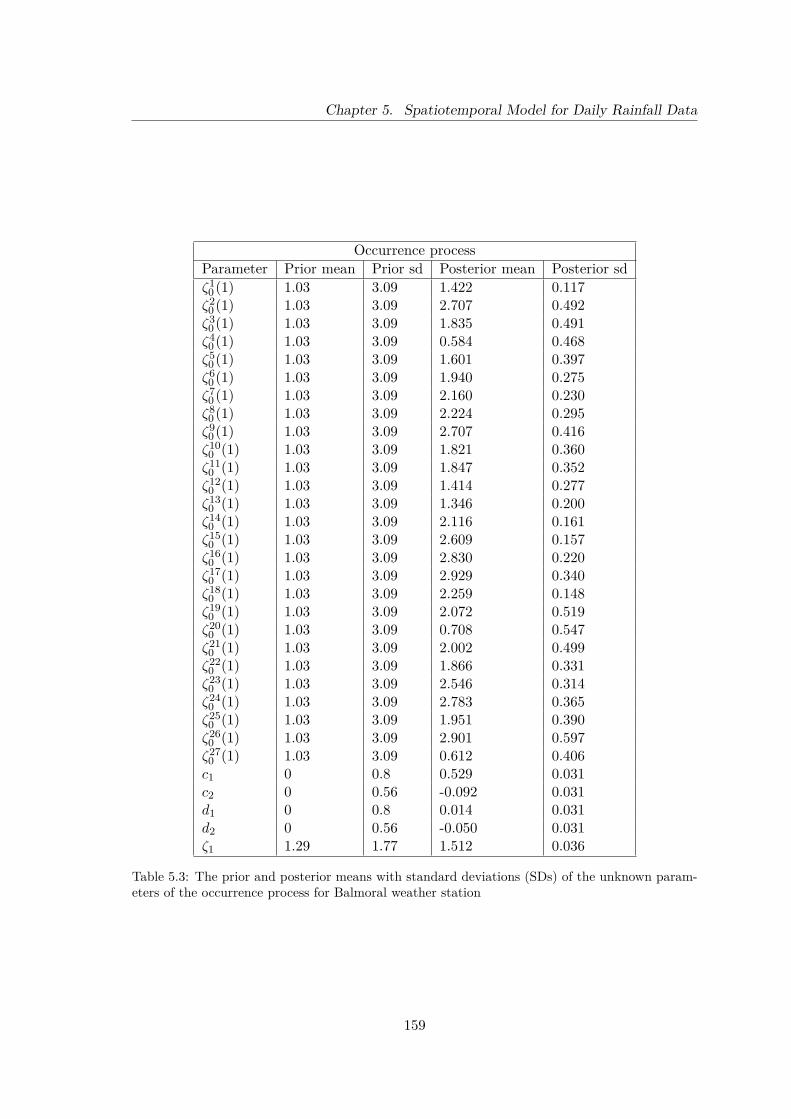
Chapter 5. Spatiotemporal Model for Daily Rainfall Data
Occurrence processParameter Prior mean Prior sd Posterior mean Posterior sdζ1
0 (1) 1.03 3.09 1.422 0.117ζ2
0 (1) 1.03 3.09 2.707 0.492ζ3
0 (1) 1.03 3.09 1.835 0.491ζ4
0 (1) 1.03 3.09 0.584 0.468ζ5
0 (1) 1.03 3.09 1.601 0.397ζ6
0 (1) 1.03 3.09 1.940 0.275ζ7
0 (1) 1.03 3.09 2.160 0.230ζ8
0 (1) 1.03 3.09 2.224 0.295ζ9
0 (1) 1.03 3.09 2.707 0.416ζ10
0 (1) 1.03 3.09 1.821 0.360ζ11
0 (1) 1.03 3.09 1.847 0.352ζ12
0 (1) 1.03 3.09 1.414 0.277ζ13
0 (1) 1.03 3.09 1.346 0.200ζ14
0 (1) 1.03 3.09 2.116 0.161ζ15
0 (1) 1.03 3.09 2.609 0.157ζ16
0 (1) 1.03 3.09 2.830 0.220ζ17
0 (1) 1.03 3.09 2.929 0.340ζ18
0 (1) 1.03 3.09 2.259 0.148ζ19
0 (1) 1.03 3.09 2.072 0.519ζ20
0 (1) 1.03 3.09 0.708 0.547ζ21
0 (1) 1.03 3.09 2.002 0.499ζ22
0 (1) 1.03 3.09 1.866 0.331ζ23
0 (1) 1.03 3.09 2.546 0.314ζ24
0 (1) 1.03 3.09 2.783 0.365ζ25
0 (1) 1.03 3.09 1.951 0.390ζ26
0 (1) 1.03 3.09 2.901 0.597ζ27
0 (1) 1.03 3.09 0.612 0.406c1 0 0.8 0.529 0.031c2 0 0.56 -0.092 0.031d1 0 0.8 0.014 0.031d2 0 0.56 -0.050 0.031ζ1 1.29 1.77 1.512 0.036
Table 5.3: The prior and posterior means with standard deviations (SDs) of the unknown param-eters of the occurrence process for Balmoral weather station
159
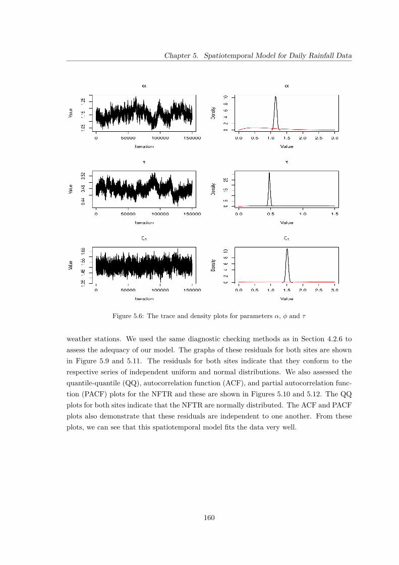
Chapter 5. Spatiotemporal Model for Daily Rainfall Data
Figure 5.6: The trace and density plots for parameters α, φ and τ
weather stations. We used the same diagnostic checking methods as in Section 4.2.6 toassess the adequacy of our model. The graphs of these residuals for both sites are shownin Figure 5.9 and 5.11. The residuals for both sites indicate that they conform to therespective series of independent uniform and normal distributions. We also assessed thequantile-quantile (QQ), autocorrelation function (ACF), and partial autocorrelation func-tion (PACF) plots for the NFTR and these are shown in Figures 5.10 and 5.12. The QQplots for both sites indicate that the NFTR are normally distributed. The ACF and PACFplots also demonstrate that these residuals are independent to one another. From theseplots, we can see that this spatiotemporal model fits the data very well.
160
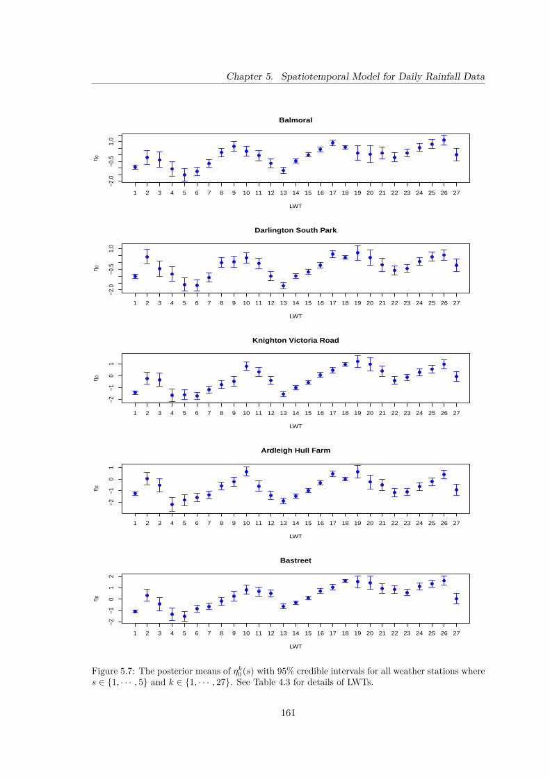
Chapter 5. Spatiotemporal Model for Daily Rainfall Data
−2.0
−0.5
1.0
Balmoral
LWT
η 0
1 2 3 4 5 6 7 8 9 10 11 12 13 14 15 16 17 18 19 20 21 22 23 24 25 26 27
−2.0
−0.5
1.0
Darlington South Park
LWT
η 0
1 2 3 4 5 6 7 8 9 10 11 12 13 14 15 16 17 18 19 20 21 22 23 24 25 26 27
−2−1
01
Knighton Victoria Road
LWT
η 0
1 2 3 4 5 6 7 8 9 10 11 12 13 14 15 16 17 18 19 20 21 22 23 24 25 26 27
−2−1
01
Ardleigh Hull Farm
LWT
η 0
1 2 3 4 5 6 7 8 9 10 11 12 13 14 15 16 17 18 19 20 21 22 23 24 25 26 27
−2−1
01
2
Bastreet
LWT
η 0
1 2 3 4 5 6 7 8 9 10 11 12 13 14 15 16 17 18 19 20 21 22 23 24 25 26 27
Figure 5.7: The posterior means of ηk0 (s) with 95% credible intervals for all weather stations where
s ∈ {1, · · · , 5} and k ∈ {1, · · · , 27}. See Table 4.3 for details of LWTs.
161

Chapter 5. Spatiotemporal Model for Daily Rainfall Data
01
23
4
Balmoral
LWT
ζ 0
1 2 3 4 5 6 7 8 9 10 11 12 13 14 15 16 17 18 19 20 21 22 23 24 25 26 27
0.0
1.0
2.0
3.0
Darlington South Park
LWT
ζ 0
1 2 3 4 5 6 7 8 9 10 11 12 13 14 15 16 17 18 19 20 21 22 23 24 25 26 27
12
34
5
Knighton Victoria Road
LWT
ζ 0
1 2 3 4 5 6 7 8 9 10 11 12 13 14 15 16 17 18 19 20 21 22 23 24 25 26 27
01
23
4
Ardleigh Hull Farm
LWT
ζ 0
1 2 3 4 5 6 7 8 9 10 11 12 13 14 15 16 17 18 19 20 21 22 23 24 25 26 27
12
34
5
Bastreet
LWT
ζ 0
1 2 3 4 5 6 7 8 9 10 11 12 13 14 15 16 17 18 19 20 21 22 23 24 25 26 27
Figure 5.8: The posterior means of ζk0 (s) with 95% credible intervals for all weather stations where
s ∈ {1, · · · , 5} and k ∈ {1, · · · , 27}. See Table 4.3 for details of LWTs.
162
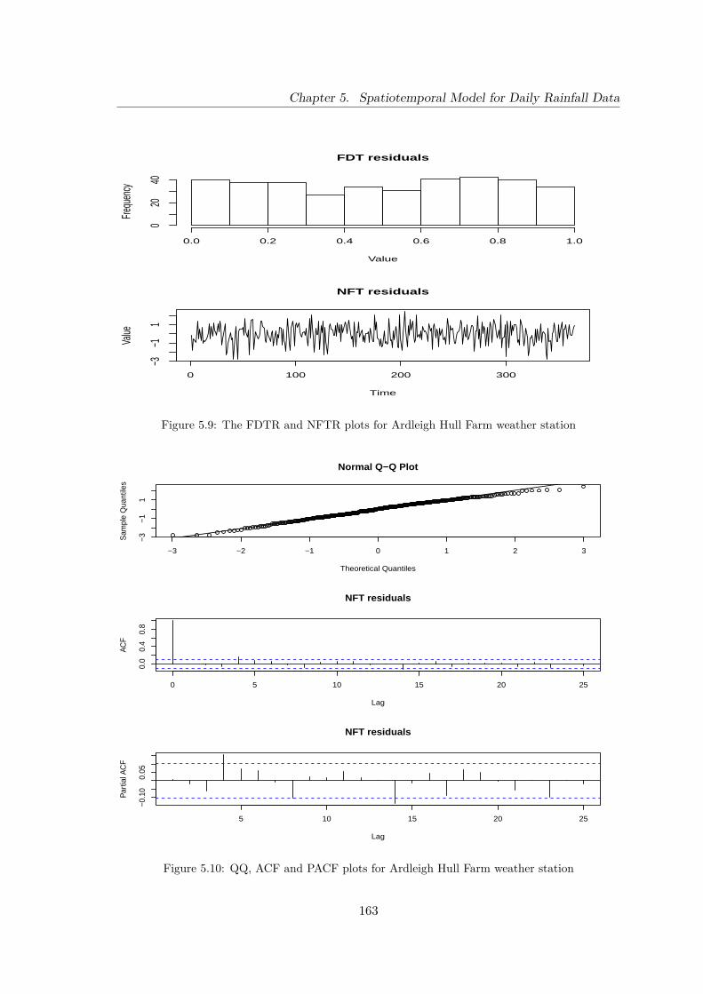
Chapter 5. Spatiotemporal Model for Daily Rainfall Data
FDT residuals
Value
Freq
uenc
y
0.0 0.2 0.4 0.6 0.8 1.0
020
40
0 100 200 300
−3−1
1
NFT residuals
Time
Value
Figure 5.9: The FDTR and NFTR plots for Ardleigh Hull Farm weather station
−3 −2 −1 0 1 2 3
−3−1
1
Normal Q−Q Plot
Theoretical Quantiles
Sam
ple
Qua
ntile
s
0 5 10 15 20 25
0.0
0.4
0.8
Lag
AC
F
NFT residuals
5 10 15 20 25
−0.1
00.
05
Lag
Par
tial A
CF
NFT residuals
Figure 5.10: QQ, ACF and PACF plots for Ardleigh Hull Farm weather station
163

Chapter 5. Spatiotemporal Model for Daily Rainfall Data
FDT residuals
Value
Freq
uenc
y
0.0 0.2 0.4 0.6 0.8 1.0
020
40
0 100 200 300
−3−1
13
NFT residuals
Time
Value
Figure 5.11: The FDTR and NFTR plots for Bastreet weather station
−3 −2 −1 0 1 2 3
−3−1
13
Normal Q−Q Plot
Theoretical Quantiles
Sam
ple
Qua
ntile
s
0 5 10 15 20 25
0.0
0.4
0.8
Lag
AC
F
NFT residuals
5 10 15 20 25
−0.1
00.
05
Lag
Par
tial A
CF
NFT residuals
Figure 5.12: QQ, ACF and PACF plots for Bastreet weather station
164

Chapter 5. Spatiotemporal Model for Daily Rainfall Data
5.8 Summary
The spatiotemporal model was presented in this chapter and applied to British dailyrainfall data at multiple sites within the UK network. This model is the extended versionof the univariate model in Chapter 4, Section 4.4 and also an alternative model to theprevious works by Heaps et al. (2015) and Germain (2010). The objective of this modelis to capture the relationship that exists between the sites and how this relationship mayaffect the daily rainfall for each site, especially when two sites are close to each other.In addition, the LWT is directly incorporated into the model through the amount andoccurrence processes since the LWT plays a crucial role in determining rainfall amountsand occurrence over the UK network.
This model is more challenging to develop than the previous univariate model in Chap-ter 4, Section 4.4 because it involves many variables and parameters to fit the data. Italso requires intensive computation to obtain the results. Based on the MCMC results inSection 5.7.2, we can consider that the proposed model fits the data very well. This isstrongly supported by the diagnostic check for the FDTR and NFTR which show that theyare independently distributed and respectively follow uniform and normal distributions.We also found high spatial correlation between sites, even at large distances in this model.From our discussion, we may consider using different types of spatial correlation functionto capture the spatial variability between sites. The amount and occurrence processesindicate that they are still highly dependent on the LWT ocurring at time t.
165
Chapter 6
Conclusion and Future Work
6.1 Conclusion
This thesis is concerned with the development of Bayesian approaches to the modelling andanalysis of univariate and multivariate time series data, especially when the observationaldistribution is a mixture distribution. Particular attention is given to the special case ofa mixture distribution which has a degenerate component at zero and another componentwith positive values and this is known as a mixed distribution. The main focus of thisresearch is to investigate and develop both univariate and multivariate models in thecase of a mixed distribution, focusing on daily rainfall data. Developing and modifyingthe work of Heaps et al. (2015) and Germain (2010) on spatiotemporal models for dailyrainfall at multiple sites is also an important feature of this research. Instead of usinghidden weather states, we applied the Lamb weather types (LWTs) directly to the model.We also used the daily rainfall dataset for the whole year in modelling the daily rainfallwith seasonal effects. This is in contrast with Heaps et al. (2015) and Germain (2010) whoonly considered winter rainfall data and excluded the seasonal effects from the model.
In Chapter 2, we presented the general concepts of time series models and Bayesianinference. We also briefly discussed the application of Bayesian inference in time seriesmodels. In Chapter 3, we introduced the basic ideas of Bayesian inference in mixturemodels, focusing on finite mixture models. Then, we presented the MCMC scheme forfinite mixture models with some discussion on the label switching problem. The case ofa mixed distribution was also discussed in this chapter and this was further expoundedin Chapters 4 and 5 using an example of daily rainfall. We also applied two differentmixture models to ultrasound data: a lognormal mixture and gamma mixture to illustratethe application of Bayesian inference in mixture models. The detailed parameterisationof the models and prior elicitation for each parameter were discussed in this chapter. We
166
Chapter 6. Conclusion and Future Work
ran an MCMC scheme using the RJAGS package to generate posterior samples for theparameters. The posterior summaries for both models were discussed and in general, theresults indicated that there is no large difference between the models.
In Chapter 4, we presented a model for a univariate time series with a mixed distri-bution applied to daily rainfall data. Firstly, we introduced the general model for dailyrainfall data in which we divided the model into two distinct processes: the amount andoccurrence processes. The amount process was used to model the amount of daily rainfall,whilst the occurrence process was used to model the probability of rainfall occurrence.In the daily rainfall model, we emphasised the relationship between the amount and oc-currence process so that no important information was lost. An important novelty inthis study is the way we deal with the seasonal effects for the daily rainfall. To achievethis, we introduced two different types of truncated Fourier series to take into accountthe seasonal variability over a year. We also constructed suitable prior distributions forthe Fourier coefficients. The diagnostic checking procedure for the mixed distribution wasalso introduced in this chapter to assess the adequacy of the model.
The general model was then applied to Italian and British daily rainfall datasets. Forthe Italian daily rainfall application, we considered three different models for the amountprocess. We found that the gamma distribution provided a slightly better fit compared tothe lognormal distribution based on the posterior mean of mean potential rainfall amountand the posterior predictive values. Therefore, we concluded that the gamma distributionis a better choice for modelling the amount process for the Italian daily rainfall data. Wecompared two different ways to model the effect of covariates on the gamma distribution.The covariate effect was applied to the scale parameter for the G1 model, whilst the effectwas applied to the shape parameter for the G2 model. Analysis of the Italian rainfall datasuggested that the shape parameter tended not to change and those effects were seen inthe scale parameter. We therefore concluded that the G1 model provided a better fit tothe observed behaviour. For the occurrence process, we used a first-order Markov chainto represent the probability of rainfall occurrence. In this parameterisation, we used themean of the amount distribution as a covariate to create a link between the amount andoccurrence processes.
For the British daily rainfall dataset, we developed and modified the previous work byHeaps et al. (2015) and Germain (2010) by incorporating atmospheric circulation patternsdirectly into the model. The atmospheric circulation patterns for the United Kingdom arerepresented by the LWTs. Based on the exploratory analysis of the British dataset, wefound a strong relationship between the LWTs and the daily rainfall data where a lowerproportion of wet days was associated with anticyclonic types and a higher proportiontended to be associated with cyclonic types. A similar relationship was found with the
167

Chapter 6. Conclusion and Future Work
mean daily rainfall amounts on wet days, where the high rainfall amounts are associatedwith cyclonic types, whilst the low level rainfall amounts are typically associated withanticyclonic types. We also developed two models for the LWTs using homogeneous andnonhomogenous first-order Markov chains. After that, we built a univariate model forBritish daily rainfall where the LWT is directly incorporated into the model through theamount and occurrence processes. We also introduced a random effect at each time t whichis conditionally dependent on the previous time t− 1 to allow for temporal variability inthe amount process parameterisation. The potential daily amounts were then fitted usinga gamma distribution. To build the relationship between the amount and occurrenceprocesses, we used the potential daily amount yt as a covariate in the parameterisation ofthe occurrence process. From the MCMC results and diagnostic checking, we found thatthe model fitted the data very well. It indicated that the potential rainfall amount andthe probability of rainfall occurrence are strongly associated with the LWTs.
In Chapter 5, we presented a spatiotemporal model for British daily rainfall usingthe data from multiple sites within the UK network. This is an extended version ofthe previous univariate model discussed in Chapter 4 and also an alternative model tothe model of Heaps et al. (2015) and Germain (2010). We also investigated the spatialcharacteristics of the dataset and we found a decreasing dependence between the rainfallamounts and occurrences as the between-site distance increases. Therefore, it is importantto add the spatial effect into the model to capture spatial variability between sites. Thecomputation of posterior distributions for the multivariate model is more challenging thanthe univariate model since it involves a large number of parameters. It also requires longercomputational time to generate posterior samples for the parameters. The adequacy ofthe model was assessed using similar diagnostic checking methods as in Chapter 4. Basedon this assessment, we found that the model provides a good fit to the data. The decayparameter also suggested that the spatial correlation falls to 0.5 when the distance betweensites is more than 578 km and this indicates high correlations between sites, even for thesites that are separated by large distances. We also found that the amount and occurrenceprocesses are highly dependent on the LWT occurring at time t, a similar characteristicto the British univariate model.
6.2 Review of objectives
The objectives of the research were stated in the beginning of this thesis as follows:
1. To investigate Bayesian time series modelling in mixed or mixture distribution ap-plications.
168
Chapter 6. Conclusion and Future Work
2. To develop novel approaches to modelling dependence, both on covariates and be-tween realisations, and how this affects both the between-component distribution(eg the occurence process in the rainfall case) and the conditional within-componentdistribution (eg for the amount process in the rainfall case).
3. To investigate the computation of posterior distributions in univariate and multi-variate models for mixture and mixed distributions.
4. To apply the developed methods to a number of practical problems and assess thestrengths and weaknesses of each approach.
We have fulfilled the first objective in Chapter 3 by presenting Bayesian inferencein mixture models. This chapter provided guidance on the general ideas and conceptsof the analysis of mixture and mixed distributions within the Bayesian framework. Forexample, we presented the MCMC scheme for mixture models to sample the posteriordistribution of parameters and auxiliary variables. We also addressed several interestingideas and issues that were relevant to mixture models such as the label switching problem.This investigation helps us to increase our understanding of Bayesian analysis in mixturemodels in terms of methodology and applications.
The development of Bayesian approaches to the modelling and analysis of univariateand multivariate time series data is the central theme of this thesis. Throughout Chapters4 and 5, we have developed univariate and multivariate models for mixed distributionusing daily rainfall data. This fulfills the second objective of this thesis. In these chapters,we give particular attention to modelling dependences, both on covariates and betweenrealisations. For instance, we have shown how the Lamb weather types (LWTs) can bedirectly incorporated into the model for the British daily rainfall. We found that thelevel of potential rainfall amount and the probability of rainfall occurrence depend on theLWTs. We also emphasised the relationship between the amount and occurrence processesfor all models by making the occurrence process dependent on the amount process.
For the computation of posterior distributions, we described the general idea in Chapter3 of an MCMC scheme to sample the posterior distribution of the parameters of mixturemodels. Thus, we use a similar technique to compute the posterior distributions for theunivariate and multivariate models for daily rainfall in Chapters 4 and 5. Both univariateand multivariate models are quite complicated. However, we found that the computationof posterior distributions for the multivariate model is more challenging since it involvesa large number of parameters which required a high computational cost to fit the model.This investigation satisfies the third objective.
Finally, the developed models are applied to the datasets in Chapters 3, 4 and 5 andthis accomplishes the fourth objective. We used the ultrasound data in Chapter 3 to
169

Chapter 6. Conclusion and Future Work
illustrate the application of mixture models. We also used the Italian and British dailyrainfall data to fit the univariate model in Chapter 4. The British univariate model isthen extended to the multivariate model in Chapter 5 by adding multiple sites withinthe United Kingdom network. We have also discussed the strengths and pitfalls of theapproaches in each chapter. For instance, the British daily rainfall model fitted the datavery well but it required a large number of iterations when running the MCMC algorithmto obtain the posterior samples.
6.3 Future work
There are several possible areas throughout this thesis where we can suggest further workusing similar concepts and methodologies. One of the possible areas is further investigationof daily rainfall using different datasets from tropical regions such as Malaysia, Indonesiaand Brazil. The tropical regions have a high average precipitation over a year which isin contrast with the temperate and subpolar regions (e.g. Italy and United Kingdom).They have also a clear pattern of wet and dry seasons over a year. For instance, inMalaysia, the wet season usually occurs between November and March and the dry seasonalways occurs from May to September. The rainfall patterns for the tropical regions areusually influenced by the El Nino Southern Oscilation (ENSO) which is a different typeof atmospheric circulation pattern. Therefore, we would endeavour to apply and extendthe methodologies in this thesis to daily rainfall data for the tropical regions. This willimprove our understanding of the rainfall impacts on flood and drought occurrences atsome specific locations.
We also recommend incorporating other physical variables such as temperature, hu-midity and wind speed into our daily rainfall model since there are strong correlationsbetween precipitation and these variables. Hence, the addition of these physical variablesmay improve the predictive accuracy and adequacy of the model. Looking at Figure 5.4a,there may be some suggestion that the spatial correlation, as the distance becomes greater,is not tending to zero. Therefore a correlation function where the limit of the correlationas the distance tends to infinity is greater than zero might be considered. For example,instead of (5.7) we could have
Σij = α+ (1− α) exp(−φ||si − sj ||)
with the additional parameter α where 0 ≤ α < 1. We can also use different typesof spatial correlation functions such as the Matern correlation function to capture thespatial variability between sites. The Matern correlation function is a popular correlationfunction that is increasingly used in spatial statistical modelling. The Matern correlation
170

Chapter 6. Conclusion and Future Work
function can be defined as follows:
Σij = 12ν−1Γ (ν)
(√νφ‖si − sj‖
)νKν
(2√νφ‖si − sj‖
)where Kν is a modified Bessel function, ν > 0 and φ are smoothness and scale parameters,respectively. We can then compare the exponential and Matern correlation functions interms of their suitability for modelling the spatial effect. The computing time for thespatiotemporal model to obtain posterior samples is quite long. Hence, it is recommendedto do future research on the computational methods to reduce computing time.
171

Appendix A
Appendix to Chapter 5
A.1 The full summaries of posterior mean and standard de-viation of the unknown parameters for the amount pro-cess
Amount processParameter Prior mean Prior SD Posterior mean Posterior SDη1
0(2) 0.69 2.83 -1.014 0.082η2
0(2) 0.69 2.83 0.409 0.271η3
0(2) 0.69 2.83 -0.451 0.275η4
0(2) 0.69 2.83 -0.849 0.268η5
0(2) 0.69 2.83 -1.628 0.245η6
0(2) 0.69 2.83 -1.663 0.203η7
0(2) 0.69 2.83 -1.102 0.164η8
0(2) 0.69 2.83 -0.018 0.181η9
0(2) 0.69 2.83 0.051 0.207η10
0 (2) 0.69 2.83 0.331 0.192η11
0 (2) 0.69 2.83 -0.067 0.197η12
0 (2) 0.69 2.83 -0.997 0.168η13
0 (2) 0.69 2.83 -1.704 0.124η14
0 (2) 0.69 2.83 -0.984 0.091η15
0 (2) 0.69 2.83 -0.688 0.088η16
0 (2) 0.69 2.83 -0.209 0.102η17
0 (2) 0.69 2.83 0.617 0.127η18
0 (2) 0.69 2.83 0.362 0.066η19
0 (2) 0.69 2.83 0.705 0.278η20
0 (2) 0.69 2.83 0.354 0.295η21
0 (2) 0.69 2.83 -0.177 0.241η22
0 (2) 0.69 2.83 -0.580 0.172
172

Appendix A. Appendix to Chapter 5
Amount processParameter Prior mean Prior SD Posterior mean Posterior SDη23
0 (2) 0.69 2.83 -0.443 0.146η24
0 (2) 0.69 2.83 0.069 0.146η25
0 (2) 0.69 2.83 0.419 0.169η26
0 (2) 0.69 2.83 0.534 0.194η27
0 (2) 0.69 2.83 -0.216 0.228η1
0(3) 0.69 2.83 -1.403 0.074η2
0(3) 0.69 2.83 -0.225 0.253η3
0(3) 0.69 2.83 -0.330 0.274η4
0(3) 0.69 2.83 -1.632 0.258η5
0(3) 0.69 2.83 -1.590 0.208η6
0(3) 0.69 2.83 -1.673 0.152η7
0(3) 0.69 2.83 -1.144 0.147η8
0(3) 0.69 2.83 -0.727 0.170η9
0(3) 0.69 2.83 -0.465 0.199η10
0 (3) 0.69 2.83 0.793 0.190η11
0 (3) 0.69 2.83 0.325 0.198η12
0 (3) 0.69 2.83 -0.379 0.154η13
0 (3) 0.69 2.83 -1.526 0.105η14
0 (3) 0.69 2.83 -0.999 0.085η15
0 (3) 0.69 2.83 -0.550 0.085η16
0 (3) 0.69 2.83 0.076 0.098η17
0 (3) 0.69 2.83 0.473 0.125η18
0 (3) 0.69 2.83 0.958 0.065η19
0 (3) 0.69 2.83 1.199 0.261η20
0 (3) 0.69 2.83 0.973 0.289η21
0 (3) 0.69 2.83 0.400 0.225η22
0 (3) 0.69 2.83 -0.398 0.163η23
0 (3) 0.69 2.83 -0.121 0.135η24
0 (3) 0.69 2.83 0.308 0.145η25
0 (3) 0.69 2.83 0.560 0.159η26
0 (3) 0.69 2.83 0.964 0.190η27
0 (3) 0.69 2.83 -0.061 0.215η1
0(4) 0.69 2.83 -1.233 0.080η2
0(4) 0.69 2.83 0.042 0.279η3
0(4) 0.69 2.83 -0.523 0.300η4
0(4) 0.69 2.83 -2.183 0.302η5
0(4) 0.69 2.83 -1.786 0.239η6
0(4) 0.69 2.83 -1.575 0.185η7
0(4) 0.69 2.83 -1.350 0.168η8
0(4) 0.69 2.83 -0.582 0.176η9
0(4) 0.69 2.83 -0.217 0.205η10
0 (4) 0.69 2.83 0.639 0.193η11
0 (4) 0.69 2.83 -0.601 0.225η12
0 (4) 0.69 2.83 -1.400 0.178η13
0 (4) 0.69 2.83 -1.877 0.129
173

Appendix A. Appendix to Chapter 5
Amount processParameter Prior mean Prior SD Posterior mean Posterior SDη14
0 (4) 0.69 2.83 -1.460 0.098η15
0 (4) 0.69 2.83 -0.986 0.089η16
0 (4) 0.69 2.83 -0.311 0.102η17
0 (4) 0.69 2.83 0.463 0.130η18
0 (4) 0.69 2.83 0.005 0.069η19
0 (4) 0.69 2.83 0.629 0.273η20
0 (4) 0.69 2.83 -0.228 0.309η21
0 (4) 0.69 2.83 -0.481 0.241η22
0 (4) 0.69 2.83 -1.144 0.188η23
0 (4) 0.69 2.83 -1.079 0.150η24
0 (4) 0.69 2.83 -0.635 0.166η25
0 (4) 0.69 2.83 -0.203 0.168η26
0 (4) 0.69 2.83 0.408 0.195η27
0 (4) 0.69 2.83 -0.906 0.239η1
0(5) 0.69 2.83 -1.068 0.076η2
0(5) 0.69 2.83 0.344 0.265η3
0(5) 0.69 2.83 -0.414 0.291η4
0(5) 0.69 2.83 -1.307 0.274η5
0(5) 0.69 2.83 -1.493 0.225η6
0(5) 0.69 2.83 -0.830 0.155η7
0(5) 0.69 2.83 -0.635 0.139η8
0(5) 0.69 2.83 -0.170 0.171η9
0(5) 0.69 2.83 0.258 0.216η10
0 (5) 0.69 2.83 0.827 0.191η11
0 (5) 0.69 2.83 0.680 0.200η12
0 (5) 0.69 2.83 0.517 0.146η13
0 (5) 0.69 2.83 -0.621 0.106η14
0 (5) 0.69 2.83 -0.306 0.088η15
0 (5) 0.69 2.83 0.113 0.080η16
0 (5) 0.69 2.83 0.721 0.097η17
0 (5) 0.69 2.83 1.041 0.128η18
0 (5) 0.69 2.83 1.620 0.068η19
0 (5) 0.69 2.83 1.542 0.269η20
0 (5) 0.69 2.83 1.439 0.293η21
0 (5) 0.69 2.83 0.938 0.217η22
0 (5) 0.69 2.83 0.858 0.164η23
0 (5) 0.69 2.83 0.582 0.140η24
0 (5) 0.69 2.83 1.130 0.149η25
0 (5) 0.69 2.83 1.348 0.157η26
0 (5) 0.69 2.83 1.628 0.188η27
0 (5) 0.69 2.83 0.045 0.224
Table A.1: The prior and posterior means with standard deviations (SDs) of the unknown param-eters of the amount process
174

Appendix A. Appendix to Chapter 5
A.2 The full summaries of posterior mean and standard de-viation of unknown parameters for the occurrence pro-cess
Occurrence processParameter Prior mean Prior SD Posterior mean Posterior SDζ1
0 (2) 1.03 3.09 0.869 0.123ζ2
0 (2) 1.03 3.09 0.759 0.476ζ3
0 (2) 1.03 3.09 1.993 0.503ζ4
0 (2) 1.03 3.09 0.697 0.436ζ5
0 (2) 1.03 3.09 1.353 0.394ζ6
0 (2) 1.03 3.09 1.048 0.307ζ7
0 (2) 1.03 3.09 1.252 0.261ζ8
0 (2) 1.03 3.09 0.681 0.288ζ9
0 (2) 1.03 3.09 1.156 0.361ζ10
0 (2) 1.03 3.09 2.050 0.363ζ11
0 (2) 1.03 3.09 1.881 0.363ζ12
0 (2) 1.03 3.09 1.339 0.283ζ13
0 (2) 1.03 3.09 1.262 0.203ζ14
0 (2) 1.03 3.09 1.307 0.155ζ15
0 (2) 1.03 3.09 1.435 0.146ζ16
0 (2) 1.03 3.09 1.725 0.178ζ17
0 (2) 1.03 3.09 1.633 0.255ζ18
0 (2) 1.03 3.09 1.644 0.135ζ19
0 (2) 1.03 3.09 1.062 0.587ζ20
0 (2) 1.03 3.09 1.787 0.615ζ21
0 (2) 1.03 3.09 1.787 0.456ζ22
0 (2) 1.03 3.09 1.603 0.327ζ23
0 (2) 1.03 3.09 1.892 0.294ζ24
0 (2) 1.03 3.09 1.811 0.299ζ25
0 (2) 1.03 3.09 1.787 0.342ζ26
0 (2) 1.03 3.09 1.546 0.403ζ27
0 (2) 1.03 3.09 1.662 0.404ζ1
0 (3) 1.03 3.09 2.918 0.140ζ2
0 (3) 1.03 3.09 4.263 0.540ζ3
0 (3) 1.03 3.09 1.927 0.527ζ4
0 (3) 1.03 3.09 2.250 0.443ζ5
0 (3) 1.03 3.09 3.118 0.365ζ6
0 (3) 1.03 3.09 3.323 0.274ζ7
0 (3) 1.03 3.09 2.914 0.251ζ8
0 (3) 1.03 3.09 2.998 0.300ζ9
0 (3) 1.03 3.09 2.692 0.377ζ10
0 (3) 1.03 3.09 3.795 0.447
175
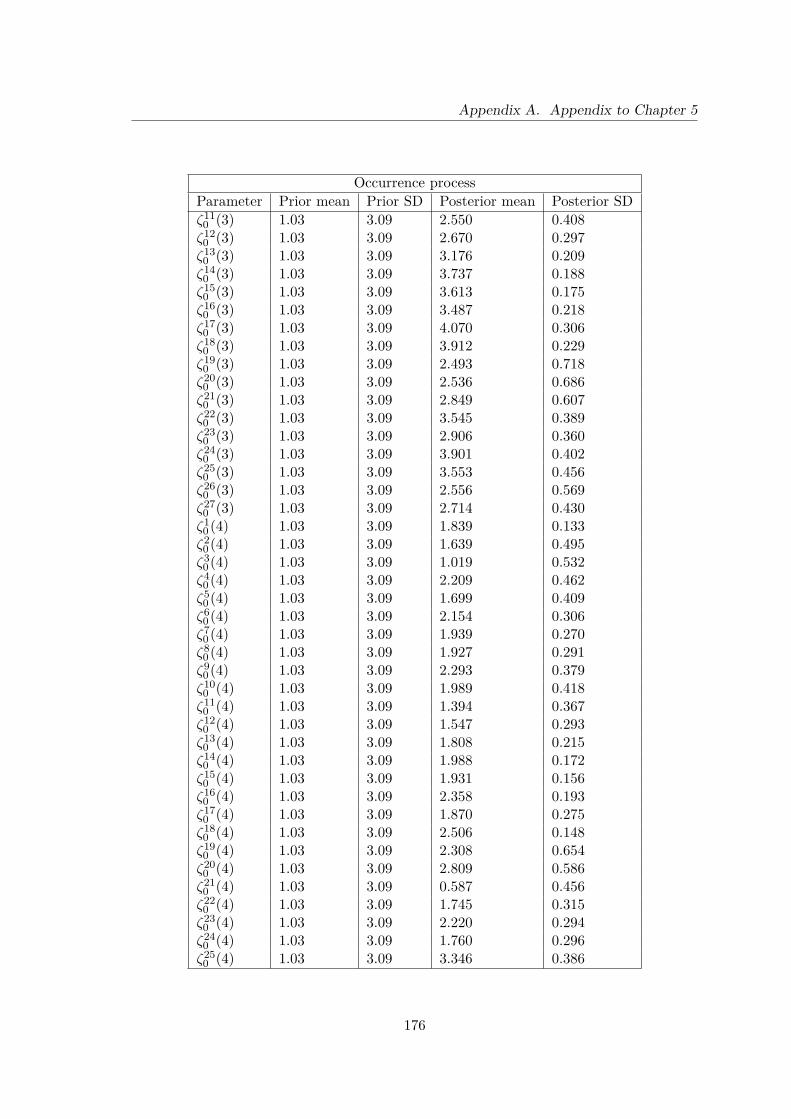
Appendix A. Appendix to Chapter 5
Occurrence processParameter Prior mean Prior SD Posterior mean Posterior SDζ11
0 (3) 1.03 3.09 2.550 0.408ζ12
0 (3) 1.03 3.09 2.670 0.297ζ13
0 (3) 1.03 3.09 3.176 0.209ζ14
0 (3) 1.03 3.09 3.737 0.188ζ15
0 (3) 1.03 3.09 3.613 0.175ζ16
0 (3) 1.03 3.09 3.487 0.218ζ17
0 (3) 1.03 3.09 4.070 0.306ζ18
0 (3) 1.03 3.09 3.912 0.229ζ19
0 (3) 1.03 3.09 2.493 0.718ζ20
0 (3) 1.03 3.09 2.536 0.686ζ21
0 (3) 1.03 3.09 2.849 0.607ζ22
0 (3) 1.03 3.09 3.545 0.389ζ23
0 (3) 1.03 3.09 2.906 0.360ζ24
0 (3) 1.03 3.09 3.901 0.402ζ25
0 (3) 1.03 3.09 3.553 0.456ζ26
0 (3) 1.03 3.09 2.556 0.569ζ27
0 (3) 1.03 3.09 2.714 0.430ζ1
0 (4) 1.03 3.09 1.839 0.133ζ2
0 (4) 1.03 3.09 1.639 0.495ζ3
0 (4) 1.03 3.09 1.019 0.532ζ4
0 (4) 1.03 3.09 2.209 0.462ζ5
0 (4) 1.03 3.09 1.699 0.409ζ6
0 (4) 1.03 3.09 2.154 0.306ζ7
0 (4) 1.03 3.09 1.939 0.270ζ8
0 (4) 1.03 3.09 1.927 0.291ζ9
0 (4) 1.03 3.09 2.293 0.379ζ10
0 (4) 1.03 3.09 1.989 0.418ζ11
0 (4) 1.03 3.09 1.394 0.367ζ12
0 (4) 1.03 3.09 1.547 0.293ζ13
0 (4) 1.03 3.09 1.808 0.215ζ14
0 (4) 1.03 3.09 1.988 0.172ζ15
0 (4) 1.03 3.09 1.931 0.156ζ16
0 (4) 1.03 3.09 2.358 0.193ζ17
0 (4) 1.03 3.09 1.870 0.275ζ18
0 (4) 1.03 3.09 2.506 0.148ζ19
0 (4) 1.03 3.09 2.308 0.654ζ20
0 (4) 1.03 3.09 2.809 0.586ζ21
0 (4) 1.03 3.09 0.587 0.456ζ22
0 (4) 1.03 3.09 1.745 0.315ζ23
0 (4) 1.03 3.09 2.220 0.294ζ24
0 (4) 1.03 3.09 1.760 0.296ζ25
0 (4) 1.03 3.09 3.346 0.386
176
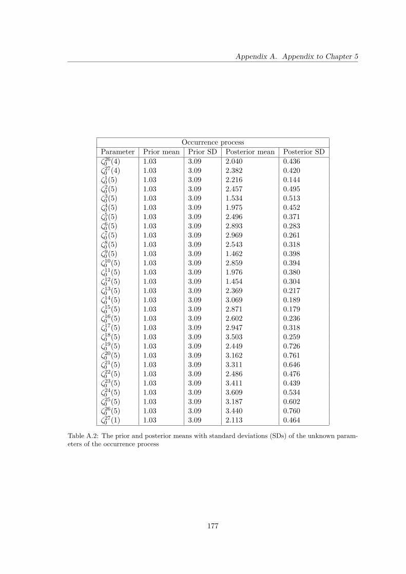
Appendix A. Appendix to Chapter 5
Occurrence processParameter Prior mean Prior SD Posterior mean Posterior SDζ26
0 (4) 1.03 3.09 2.040 0.436ζ27
0 (4) 1.03 3.09 2.382 0.420ζ1
0 (5) 1.03 3.09 2.216 0.144ζ2
0 (5) 1.03 3.09 2.457 0.495ζ3
0 (5) 1.03 3.09 1.534 0.513ζ4
0 (5) 1.03 3.09 1.975 0.452ζ5
0 (5) 1.03 3.09 2.496 0.371ζ6
0 (5) 1.03 3.09 2.893 0.283ζ7
0 (5) 1.03 3.09 2.969 0.261ζ8
0 (5) 1.03 3.09 2.543 0.318ζ9
0 (5) 1.03 3.09 1.462 0.398ζ10
0 (5) 1.03 3.09 2.859 0.394ζ11
0 (5) 1.03 3.09 1.976 0.380ζ12
0 (5) 1.03 3.09 1.454 0.304ζ13
0 (5) 1.03 3.09 2.369 0.217ζ14
0 (5) 1.03 3.09 3.069 0.189ζ15
0 (5) 1.03 3.09 2.871 0.179ζ16
0 (5) 1.03 3.09 2.602 0.236ζ17
0 (5) 1.03 3.09 2.947 0.318ζ18
0 (5) 1.03 3.09 3.503 0.259ζ19
0 (5) 1.03 3.09 2.449 0.726ζ20
0 (5) 1.03 3.09 3.162 0.761ζ21
0 (5) 1.03 3.09 3.311 0.646ζ22
0 (5) 1.03 3.09 2.486 0.476ζ23
0 (5) 1.03 3.09 3.411 0.439ζ24
0 (5) 1.03 3.09 3.609 0.534ζ25
0 (5) 1.03 3.09 3.187 0.602ζ26
0 (5) 1.03 3.09 3.440 0.760ζ27
0 (1) 1.03 3.09 2.113 0.464
Table A.2: The prior and posterior means with standard deviations (SDs) of the unknown param-eters of the occurrence process
177

References
Al-Awadhi, S. A. & Garthwaite, P. H. 1998 An elicitation method for multivariatenormal distributions. Communications in Statistics – Theory and Methods 27, 1123–1142.
Al-Awadhi, S. A. & Garthwaite, P. H. 2001 Prior distribution assessment for amultivariate normal distribution: An experimental study. Journal of Applied Statistics28, 5–23.
de Alba, E. 1993 Constrained forecasting in autoregressive time series models: ABayesian analysis. International Journal of Forecasting 9 (1), 95–108.
Azzalini, A. & Bowman, A. W. 1990 A look at some data on the old faithful geyser.Applied Statistics 39 (3), 357.
Banerjee, S., Carlin, B. & Gelfand, A. 2004 Hierarchical Modeling and Analysis forSpatial Data. CRC Press.
Barry, R. G. & Chorley, R. J. 2003 Atmosphere, weather, and climate, 8th edn.London : Routledge.
Ben-Gai, T., Bitan, A., Manes, A., Alpert, P. & Rubin, S. 1998 Spatial andtemporal changes in rainfall frequency distribution patterns in Israel. Theoretical andApplied Climatology 61 (3), 177–190.
Bennett, J., Racine-Poon, A. & Wakefiled, J. 1996 MCMC for non-linear hierar-chical models. In Markov chain Monte Carlo in practice (ed. W. R. Gilks, S. Richardson& D. J. Spiegelhalter), pp. 339–357. Chapman & Hall/CRC.
Besag, J. 1974 Spatial interaction and the statistical analysis of lattice systems. Journalof the Royal Statistical Society. Series B (Methodological) 36 (2), 192–236.
Besag, J., Green, P., Higdon, D. & Mengersen, K. 1995 Bayesian computation instochastic systems. Statistical Science 10, 3–66.
178
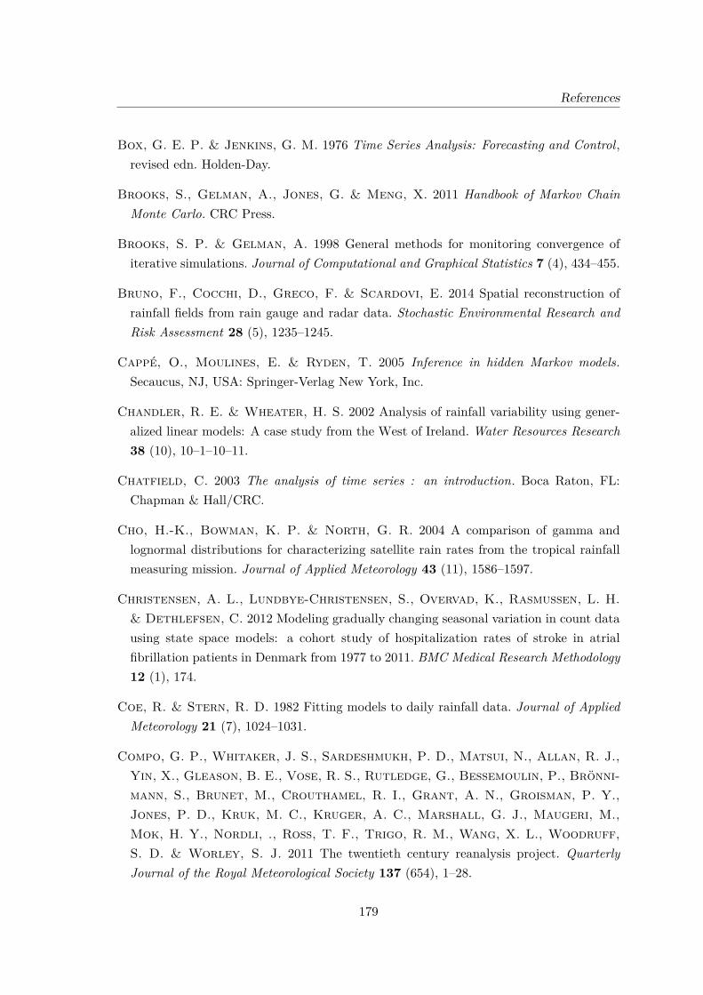
References
Box, G. E. P. & Jenkins, G. M. 1976 Time Series Analysis: Forecasting and Control,revised edn. Holden-Day.
Brooks, S., Gelman, A., Jones, G. & Meng, X. 2011 Handbook of Markov ChainMonte Carlo. CRC Press.
Brooks, S. P. & Gelman, A. 1998 General methods for monitoring convergence ofiterative simulations. Journal of Computational and Graphical Statistics 7 (4), 434–455.
Bruno, F., Cocchi, D., Greco, F. & Scardovi, E. 2014 Spatial reconstruction ofrainfall fields from rain gauge and radar data. Stochastic Environmental Research andRisk Assessment 28 (5), 1235–1245.
Cappe, O., Moulines, E. & Ryden, T. 2005 Inference in hidden Markov models.Secaucus, NJ, USA: Springer-Verlag New York, Inc.
Chandler, R. E. & Wheater, H. S. 2002 Analysis of rainfall variability using gener-alized linear models: A case study from the West of Ireland. Water Resources Research38 (10), 10–1–10–11.
Chatfield, C. 2003 The analysis of time series : an introduction. Boca Raton, FL:Chapman & Hall/CRC.
Cho, H.-K., Bowman, K. P. & North, G. R. 2004 A comparison of gamma andlognormal distributions for characterizing satellite rain rates from the tropical rainfallmeasuring mission. Journal of Applied Meteorology 43 (11), 1586–1597.
Christensen, A. L., Lundbye-Christensen, S., Overvad, K., Rasmussen, L. H.& Dethlefsen, C. 2012 Modeling gradually changing seasonal variation in count datausing state space models: a cohort study of hospitalization rates of stroke in atrialfibrillation patients in Denmark from 1977 to 2011. BMC Medical Research Methodology12 (1), 174.
Coe, R. & Stern, R. D. 1982 Fitting models to daily rainfall data. Journal of AppliedMeteorology 21 (7), 1024–1031.
Compo, G. P., Whitaker, J. S., Sardeshmukh, P. D., Matsui, N., Allan, R. J.,Yin, X., Gleason, B. E., Vose, R. S., Rutledge, G., Bessemoulin, P., Bronni-mann, S., Brunet, M., Crouthamel, R. I., Grant, A. N., Groisman, P. Y.,Jones, P. D., Kruk, M. C., Kruger, A. C., Marshall, G. J., Maugeri, M.,Mok, H. Y., Nordli, ., Ross, T. F., Trigo, R. M., Wang, X. L., Woodruff,S. D. & Worley, S. J. 2011 The twentieth century reanalysis project. QuarterlyJournal of the Royal Meteorological Society 137 (654), 1–28.
179

References
Cowburn, G. J., Parker, N. G. & Farrow, M. 2018 Bayesian inference for fluctuatingultrasonic pulse-echo measurements. In preparation.
Cowles, M. K. & Carlin, B. P. 1996 Markov chain Monte Carlo convergence diagnos-tics: A comparative review. Journal of the American Statistical Association 91 (434),883–904.
Delmar, P., Robin, S. & Daudin, J. J. 2004 VarMixt: efficient variance modellingfor the differential analysis of replicated gene expression data. Bioinformatics 21 (4),502–508.
Durbin, J. & Koopman, S. J. 2000 Time series analysis of non-Gaussian observationsbased on state space models from both classical and Bayesian perspectives. Journal ofthe Royal Statistical Society B 62, 3–56.
Farrow, M. 2003 Practical building of subjective covariance structures for large compli-cated systems. The Statistician 52, 553–573.
Fernandes, M. V., Schmidt, A. M. & Migon, H. S. 2009 Modelling zero-inflatedspatio-temporal processes. Statistical Modelling 9 (1), 3–25.
Fruhwirth-Schnatter, S. 2006 Finite mixture and Markov switching models. Springer.
Furrer, E. & Katz, R. 2007 Generalized linear modeling approach to stochastic weathergenerators. Climate Research 34, 129–144.
Gabriel, K. R. & Neumann, J. 1962 A Markov chain model for daily rainfall occurrenceat Tel Aviv. Quarterly Journal of the Royal Meteorological Society 88 (375), 90–95.
Gamerman, D. 1997 Sampling from the posterior distribution in generalized linear mixedmodels. Statistics and Computing 7 (1), 57–68.
Gamerman, D. & Lopes, H. F. 2006 Markov chain Monte Carlo : stochastic simulationfor Bayesian inference. Boca Raton: Taylor & Francis.
Garthwaite, P. H., Kadane, J. B. & O’Hagan, A. 2005 Statistical methods for elicit-ing probability distributions. Journal of the American Statistical Association 100 (470),680–701.
Gelfand, A. E. & Smith, A. F. M. 1990 Sampling-based approaches to calculatingmarginal densities. Journal of the American Statistical Association 85 (410), 398–409.
Gelman, A., Roberts, G. & Gilks, W. 1996 Efficient Metropolis jumping rules. InBayesian Statistics (ed. J. M. Bernado et al.), pp. 599–607. OUP.
180

References
Gelman, A. & Rubin, D. B. 1992 Inference from iterative simulation using multiplesequences. Statist. Sci. 7 (4), 457–472.
Geman, S. & Geman, D. 1984 Stochastic relaxation, Gibbs distribution, and theBayesian restoration of images. IEEE Transactions on Pattern Recognition 6, 721–741.
Germain, S. E. 2010 Bayesian spatio-temporal modelling of rainfall through non-homogeneous hidden Markov models. PhD thesis, School of Mathematics & Statistics,Newcastle University, UK.
Geweke, J. 1992 Evaluating the accuracy of sampling-based approaches to the calculationof posterior moments. In IN BAYESIAN STATISTICS , pp. 169–193. University Press.
Glickman, T. S. 2000 Glossary of meteorology. American Meteorological Society.
Grunwald, G. K. & Jones, R. H. 2000 Markov models for time series with mixeddistribution. Environmetrics 11 (3), 327–339.
Harrison, P. J. & Stevens, C. F. 1971 A Bayesian approach to short-term forecasting.Journal of the Operational Research Society 22 (4), 341–362.
Harrison, P. J. & Stevens, C. F. 1976 Bayesian forecasting. Journal of the RoyalStatistical Society. Series B (Methodological) 38 (3), 205–247.
Hastings, W. K. 1970 Monte Carlo sampling methods using Markov chains and theirapplications. Biometrika 57 (1), 97–109.
Hay, L. E., McCabe, G. J., Wolock, D. M. & Ayers, M. A. 1991 Simulation ofprecipitation by weather type analysis. Water Resources Research 27 (4), 493–501.
Heaps, S. E., Boys, R. J. & Farrow, M. 2015 Bayesian modelling of rainfall data byusing non-homogeneous hidden Markov models and latent Gaussian variables. Journalof the Royal Statistical Society: Series C (Applied Statistics) 71, 543–568.
Heidelberger, P. & Welch, P. D. 1983 Simulation run length control in the presenceof an initial transient. Operations Research 31 (6), 1109–1144.
Hess, P. & Brezowsky, H. 1969 Katalog der Grosswetterlagen Europas. D.W.
Jasra, A., Holmes, C. C. & Stephens, D. A. 2005 Markov chain Monte Carlo methodsand the label switching problem in Bayesian mixture modeling. Statist. Sci. 20 (1), 50–67.
Jenkinson, A. F. & Collinson, B. P. 1977 An initial climatology of gales over theNorth Sea. Synoptic climatology branch memorandum 62. Meteorological Office, Brack-nell, UK.
181

References
Jimoh, O. & Webster, P. 1996 The optimum order of a Markov chain model for dailyrainfall in Nigeria. Journal of Hydrology 185 (1), 45 – 69.
Jones, P. D., Harpham, C. & Briffa, K. R. 2013 Lamb weather types derived fromreanalysis products. International Journal of Climatology 33 (5), 1129–1139.
Jones, R. H. & Brelsford, W. M. 1967 Time series with periodic structure. Biometrika54 (3-4), 403–408.
Kadane, J. & Wolfson, L. J. 1998 Experiences in elicitation. Journal of the RoyalStatistical Society: Series D (The Statistician) 47 (1), 3–19.
Kalman, R. E. & Bucy, R. S. 1961 New results in linear filtering and prediction theory.Journal of Basic Engineering 83 (1), 95.
Kalnay, E., Kanamitsu, M., Kistler, R., Collins, W., Deaven, D., Gandin,L., Iredell, M., Saha, S., White, G., Woollen, J., Zhu, Y., Leetmaa, A.,Reynolds, R., Chelliah, M., Ebisuzaki, W., Higgins, W., Janowiak, J.,Mo, K. C., Ropelewski, C., Wang, J., Jenne, R. & Joseph, D. 1996 TheNCEP/NCAR 40-year reanalysis project. Bulletin of the American Meteorological Soci-ety 77 (3), 437–471.
Katz, R. W. 1977 Precipitation as a chain-dependent process. Journal of Applied Mete-orology 16 (7), 671–676.
Kendall, D. G. 1953 Stochastic processes occurring in the theory of queues and theiranalysis by the method of the imbedded Markov chain. The Annals of MathematicalStatistics 24 (3), 338–354.
Kitagawa, G. 1998 A self-organizing state-space model. Journal of the American Statis-tical Association 93 (443), 1203.
Knorr-Held, L. & Besag, J. 1998 Modelling risk from a disease in time and space.Statistics in Medicine 17 (18), 2045–2060.
Kong, A., Liu, J. S. & Wong, W. H. 1994 Sequential imputations and Bayesian missingdata problems. Journal of the American Statistical Association 89 (425), 278.
Lamb, H. H. 1972 British Isles weather types and a register of the daily sequence ofcirculation patterns 1861-1971 . H.M. Stationery Off.
Lima, C. H. R. & Lall, U. 2009 Hierarchical Bayesian modeling of multisite daily rainfalloccurrence: Rainy season onset, peak, and end. Water Resources Research 45 (7).
182

References
Liu, Y., Zhang, W., Shao, Y. & Zhang, K. 2011 A comparison of four precipitationdistribution models used in daily stochastic models. Advances in Atmospheric Sciences28 (4), 809–820.
Lunn, D., Jackson, C., Best, N., Thomas, A. & Spiegelhalter, D. 2012 TheBUGS Book: A Practical Introduction to Bayesian Analysis. London: Chapman andHall.
Marin, J.-M., Mengersen, K. & Robert, C. P. 2005 Bayesian modelling and infer-ence on mixtures of distributions. Handbook of Statistics 25, (D. Dey and C. R. Rao,eds.) volume 25 (to appear), 15840–15845.
Masson, P. R. 2001 Exchange rate regime transitions. Journal of Development Eco-nomics 64 (2), 571–586.
Matern, B. 1986 Spatial Variation, 2nd edn. Berlin: Springer-Verlag.
McCullagh, P. & Nelder, J. A. 1989 Generalized linear models (Second edition).London: Chapman & Hall.
McLachlan, G. & Peel, D. 2001 Finite mixture models. Wiley.
Met Office 2017 Meteorological Office land surface stations observations 2017. http:
//data.ceda.ac.uk/badc/ukmo-surface/data/united_kingdom/.
Metropolis, N., Rosenbluth, A. W., Rosenbluth, M. N., Teller, A. H. &Teller, E. 1953 Equation of state calculations by fast computing machines. The Jour-nal of Chemical Physics 21 (6), 1087–1092.
Monahan, J. F. 1983 Fully Bayesian analysis of ARMA time series models. Journal ofEconometrics 21 (3), 307–331.
Nelder, J. A. & Wedderburn, R. W. M. 1972 Generalized linear models. Journal ofthe Royal Statistical Society, Series A, General 135, 370–384.
Newcomb, S. 1886 A generalized theory of the combination of observations so as toobtain the best result. American Journal of Mathematics 8 (4), 343.
O’Hagan, A. 1998 Eliciting expert beliefs in substantial practical applications. Journalof the Royal Statistical Society: Series D (The Statistician) 47 (1), 21–35.
O’Hagan, A., Buck, C. E., Daneshkhah, A., Eiser, J. R., Garthwaite, P. H.,Jenkinson, D. J., Oakley, J. E. & Rakow, T. 2006 Uncertain Judgements: Elic-iting Expert Probabilities. Chichester: John Wiley.
183
References
Pearson, K. 1894 Contributions to the mathematical theory of evolution. PhilosophicalTransactions of the Royal Society A: Mathematical, Physical and Engineering Sciences185 (0), 71–110.
Petris, G., Petrone, S. & Campagnoli, P. 2009 Dynamic linear models with R.Dordrecht New York: Springer-Verlag.
Plummer, M. 2012 Bayesian Graphical Models using MCMC , 3rd edn. CRAN.
Puolamaki, K. & Kaski, S. 2009 Bayesian solutions to the label switching problem.Lecture Notes in Computer Science 5772 LCNS, 381–392, cited By 1.
R Development Core Team 2008 R: A Language and Environment for StatisticalComputing. R Foundation for Statistical Computing, Vienna, Austria, ISBN 3-900051-07-0.
Raftery, A. E. & Lewis, S. 1992 How many iterations in the Gibbs sampler? InBayesian Statistics 4 , pp. 763–773. Oxford University Press.
Redner, R. A. & Walker, H. F. 1984 Mixture densities, maximum likelihood and theEM algorithm. SIAM Rev. 26 (2), 195–239.
Reich, B. J., Hodges, J. S. & Zadnik, V. 2006 Effects of residual smoothing on theposterior of the fixed effects in disease-mapping models. Biometrics 62 (4), 1197–1206.
Richardson, C. W. 1981 Stochastic simulation of daily precipitation, temperature, andsolar radiation. Water Resources Research 17 (1), 182–190.
Roldan, J. & Woolhiser, D. A. 1982 Stochastic daily precipitation models: 1. Acomparison of occurrence processes. Water Resources Research 18 (5), 1451–1459.
Rosenberg, M. A. & Young, V. R. 1999 A Bayesian approach to understanding timeseries data. North American Actuarial Journal 3 (2), 130–143.
Sanso, B. & Guenni, L. 1999 A stochastic model for tropical rainfall at a single location.Journal of Hydrology 214 (1-4), 64–73.
Scott, S. L. 2002 Bayesian methods for hidden Markov models. Journal of the AmericanStatistical Association 97 (457), 337–351.
Smith, J. Q. 1985 Diagnostic checks of non-standard time series models. Journal ofForecasting 4 (3), 283–291.
Sofia, S. 2007 Nonlinear time-series models for Mediterranean rainfall data with zeroes.PhD thesis, University of Sunderland, UK.
184
References
Stephens, M. 2000 Dealing with label switching in mixture models. Journal of the RoyalStatistical Society: Series B (Statistical Methodology) 62 (4), 795–809.
Stern, R. D. & Coe, R. 1984 A model fitting analysis of daily rainfall data. Journal ofthe Royal Statistical Society. Series A (General) 147 (1), 1.
Stewart, W. 2009 Probability, Markov chains, queues, and simulation : the mathematicalbasis of performance modeling. Princeton, N.J: Princeton University Press.
Suhaila, J., Ching-Yee, K., Fadhilah, Y. & Hui-Mean, F. 2011 Introducing themixed distribution in fitting rainfall data. Open Journal of Modern Hydrology 01 (02),11–22.
Tadesse, M. G., Sha, N. & Vannucci, M. 2005 Bayesian variable selection in clusteringhigh-dimensional data. Journal of the American Statistical Association 100 (470), 602–617.
Tanner, M. A. & Wong, W. H. 1987 The calculation of posterior distributions by dataaugmentation. Journal of the American Statistical Association 82 (398), 528.
Thompson, C. S., Thomson, P. J. & Zheng, X. 2007 Fitting a multisite daily rainfallmodel to New Zealand data. Journal of Hydrology 340 (1), 25 – 39.
Tooze, J. A., Grunwald, G. K. & Jones, R. H. 2002 Analysis of repeated measuresdata with clumping at zero. Statistical Methods in Medical Research 11 (4), 341–355.
Velarde, L. G. C., Migon, H. S. & Pereira, B. d. B. 2004 Space–time modeling ofrainfall data. Environmetrics 15 (6), 561–576.
Waller, L. A. & Carlin, B. P. 2010 Disease mapping. Chapman Hall CRC HandbMod Stat Methods 2010, 217–243.
West, M. & Harrison, J. 1997 Bayesian forecasting and dynamic methods. Springer-Verlag.
West, M., Harrison, P. J. & Migon, H. S. 1985 Dynamic generalised linear modelsand Bayesian forecasting (with discussion). Journal of the American Statistical Associ-ation 80, 73–97.
Wilks, D. 1999 Interannual variability and extreme-value characteristics of severalstochastic daily precipitation models. Agricultural and Forest Meteorology 93 (3), 153–169.
Winkler, R. L. 1967 The assessment of prior distributipons in Bayesian analysis. Journalof the American Statistical Association 62, 776–880.
185
References
Yang, C., Chandler, R. E., Isham, V. S. & Wheater, H. S. 2005 Spatial-temporalrainfall simulation using generalized linear models. Water Resources Research 41 (11),w11415.
Yarnal, B. 1993 Synoptic climatology in environmental analysis : a primer . BelhavenPress London ; Boca Raton, Fla.
Zellner, A. 1971 An introduction to Bayesian inference in econometrics. John Wiley.
Zucchini, W. 2009 Hidden Markov models for time series : an introduction using R.Boca Raton: CRC Press/Taylor & Francis Group.
186


