Bayesian k-nearest-neighbour classificationjunliu/Workshops/workshop2007/talk... · Bayesian...
97
Bayesian k-nearest-neighbour classification Bayesian k-nearest-neighbour classification Christian P. Robert Universit´ e Paris Dauphine & CREST, INSEE http://www.ceremade.dauphine.fr/ ∼ xian Joint work with G. Celeux, J.M. Marin, & D.M. Titterington
Transcript of Bayesian k-nearest-neighbour classificationjunliu/Workshops/workshop2007/talk... · Bayesian...
Bayesian k-nearest-neighbour classification
Bayesian k-nearest-neighbour classification
Christian P. Robert
Universite Paris Dauphine & CREST, INSEE
http://www.ceremade.dauphine.fr/∼xian
Joint work with G. Celeux, J.M. Marin, & D.M. Titterington

Bayesian k-nearest-neighbour classification
Outline
1 MRFs
2 Bayesian inference in Gibbs random fields
3 Perfect sampling
4 k-nearest-neighbours
5 Pseudo-likelihood reassessed
6 Variable selection
Bayesian k-nearest-neighbour classification
MRFs
MRFs
Markov random fields: natural spatial generalisation of Markovchains

Bayesian k-nearest-neighbour classification
MRFs
MRFs
Markov random fields: natural spatial generalisation of Markovchains
They can be derived from graph structures, when ignoring timedirectionality/causality
E.g., a Markov chain is also a chain graph of random variables,where each variable in the graph has the property that it isindependent of all (both past and future) others given its twonearest neighbours.
Bayesian k-nearest-neighbour classification
MRFs
MRFs (cont’d)
Definition (MRF)
A general Markov random field is the extension of the above toany graph structure on the random variables, i.e., a collection ofrv’s such that each one is independent of all the others given itsimmediate neighbours in the corresponding graph.
[Cressie, 1993]
Bayesian k-nearest-neighbour classification
MRFs
A formal definition
Take y1, . . . , yn, rv’s with values in a finite set S, and letG = (N, E) be a finite graph with N = {1, ..., n} the collection ofnodes and E the collection of edges, made of pairs from N .
Bayesian k-nearest-neighbour classification
MRFs
A formal definition
Take y1, . . . , yn, rv’s with values in a finite set S, and letG = (N, E) be a finite graph with N = {1, ..., n} the collection ofnodes and E the collection of edges, made of pairs from N .For A ⊆ N , δA denotes the set of neighbours of A, i.e. thecollection of all points in N/A that have a neighbour in A.
Definition (MRF)
y = (y1, . . . , yn) is a Markov random field associated with thegraph G if its full conditionals satisfy
f (yi|y−i) = f (yi|yδi) .
Cliques are sets of points that are all neighbours of one another.
Bayesian k-nearest-neighbour classification
MRFs
Gibbs distributions
Special case of MRF:
Bayesian k-nearest-neighbour classification
MRFs
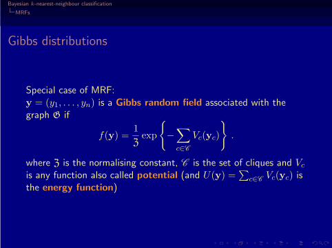
Gibbs distributions
Special case of MRF:y = (y1, . . . , yn) is a Gibbs random field associated with thegraph G if
f(y) =1
Zexp
{−
∑
c∈C
Vc(yc)
}.
where Z is the normalising constant, C is the set of cliques and Vc
is any function also called potential (and U(y) =∑
c∈CVc(yc) is
the energy function)

Bayesian k-nearest-neighbour classification
MRFs
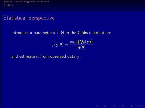
Statistical perspective
Introduce a parameter θ ∈ Θ in the Gibbs distribution:
f(y|θ) =exp {Qθ(y)}
Z(θ)
Bayesian k-nearest-neighbour classification
MRFs
Statistical perspective
Introduce a parameter θ ∈ Θ in the Gibbs distribution:
f(y|θ) =exp {Qθ(y)}
Z(θ)
and estimate it from observed data y.
Bayesian k-nearest-neighbour classification
MRFs
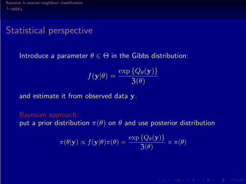
Statistical perspective
Introduce a parameter θ ∈ Θ in the Gibbs distribution:
f(y|θ) =exp {Qθ(y)}
Z(θ)
and estimate it from observed data y.
Bayesian approach:put a prior distribution π(θ) on θ and use posterior distribution
π(θ|y) ∝ f(y|θ)π(θ) =exp {Qθ(y)}
Z(θ)× π(θ)

Bayesian k-nearest-neighbour classification
MRFs
Potts model
Example (Boltzman dependence)
Case when Qθ(y) is of the form
Qθ(y) = θS(y)
= θ∑
l∼ki
δyl=yi
Path for Potts
Bayesian k-nearest-neighbour classification
Bayesian inference in Gibbs random fields
1 MRFs
2 Bayesian inference in Gibbs random fieldsPseudo-posterior inferencePath samplingAuxiliary variables
3 Perfect sampling
4 k-nearest-neighbours
5 Pseudo-likelihood reassessed
6 Variable selection

Bayesian k-nearest-neighbour classification
Bayesian inference in Gibbs random fields
Bayesian inference in Gibbs random fields
Use the posterior π(θ|y) to draw inference
Bayesian k-nearest-neighbour classification
Bayesian inference in Gibbs random fields
Bayesian inference in Gibbs random fields
Use the posterior π(θ|y) to draw inferenceProblem
Z(θ) =∑
y
exp {Qθ(y)}
not available analytically & exact computation not feasible.
Bayesian k-nearest-neighbour classification
Bayesian inference in Gibbs random fields
Bayesian inference in Gibbs random fields
Use the posterior π(θ|y) to draw inferenceProblem
Z(θ) =∑
y
exp {Qθ(y)}
not available analytically & exact computation not feasible.
Solutions:
Pseudo-posterior inference
Path sampling approximations
Auxiliary variable method
Bayesian k-nearest-neighbour classification
Bayesian inference in Gibbs random fields
Pseudo-posterior inference
Pseudo-posterior inference
Oldest solution: replace the likelihood with the pseudo-likelihood
pseudo-like(y|θ) =
n∏
i=1
f(yi|y−i, θ) .
Then define pseudo-posterior
pseudo-post(θ|y) ∝n∏
i=1
f(yi|y−i, θ)π(θ)
and resort to MCMC methods to derive a sample from pseudo-post[Besag, 1974-75]

Bayesian k-nearest-neighbour classification
Bayesian inference in Gibbs random fields
Path sampling
Path sampling
Generate a sample from [the true] π(θ|y) by aMetropolis-Hastings algorithm, with acceptance probability
MH1(θ′|θ) =
{Z(θ)
Z(θ′)
} {exp [Qθ′(y)] π(θ′)
exp [Qθ(y)] π(θ)
} {q1(θ|θ
′)
q1(θ′|θ)
}
where q1(θ′|θ) is a [arbitrary] proposal density.
[Robert & Casella, 1999/2004]
Bayesian k-nearest-neighbour classification
Bayesian inference in Gibbs random fields
Path sampling
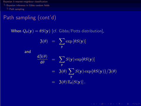
Path sampling (cont’d)
When Qθ(y) = θS(y) [cf. Gibbs/Potts distribution],
Z(θ) =∑
y
exp [θS(y)]
anddZ(θ)
dθ=
∑
y
S(y) exp[θS(y)]
= Z(θ)∑
y
S(y) exp{θS(y)}/Z(θ)
= Z(θ) Eθ[S(y)] .
Bayesian k-nearest-neighbour classification
Bayesian inference in Gibbs random fields
Path sampling
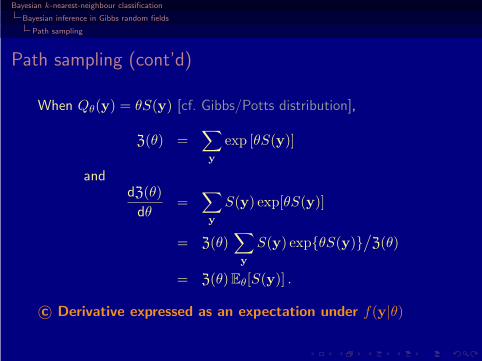
Path sampling (cont’d)
When Qθ(y) = θS(y) [cf. Gibbs/Potts distribution],
Z(θ) =∑
y
exp [θS(y)]
anddZ(θ)
dθ=
∑
y
S(y) exp[θS(y)]
= Z(θ)∑
y
S(y) exp{θS(y)}/Z(θ)
= Z(θ) Eθ[S(y)] .
c© Derivative expressed as an expectation under f(y|θ)

Bayesian k-nearest-neighbour classification
Bayesian inference in Gibbs random fields
Path sampling
Path sampling identity
Therefore, the ratio Z(θ)/Z(θ′) can be derived from an integral,since
log
{Z(θ)
Z(θ′)
}=
∫ θ′
θ
Eu[S(y)]du .
[Gelman & Meng, 1998]
Bayesian k-nearest-neighbour classification
Bayesian inference in Gibbs random fields
Path sampling
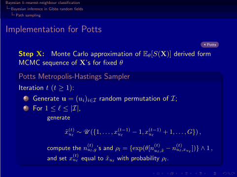
Implementation for Potts
Potts
Step X: Monte Carlo approximation of Eθ[S(X)] derived formMCMC sequence of X’s for fixed θ
Potts Metropolis-Hastings Sampler
Iteration t (t ≥ 1):
1 Generate u = (ui)i∈I random permutation of I;2 For 1 ≤ ℓ ≤ |I|,
generate
x(t)uℓ
∼ U ({1, . . . , x(t−1)uℓ
− 1, x(t−1)uℓ
+ 1, . . . , G}) ,
compute the n(t)ul,g’s and ρl = {exp(θ[n
(t)uℓ,x − n
(t)uℓ,xuℓ
])} ∧ 1 ,
and set x(t)uℓ
equal to xuℓwith probability ρl.
Bayesian k-nearest-neighbour classification
Bayesian inference in Gibbs random fields
Path sampling
Implementation for Potts (2)
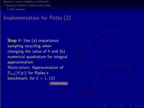
Step θ: Use (a) importancesampling recycling whenchanging the value of θ and (b)numerical quadrature for integralapproximation
Bayesian k-nearest-neighbour classification
Bayesian inference in Gibbs random fields
Path sampling
Implementation for Potts (2)
Step θ: Use (a) importancesampling recycling whenchanging the value of θ and (b)numerical quadrature for integralapproximationIllustration: Approximation ofEβ,k[S(y)] for Ripley’sbenchmark, for k = 1, 125
Perfect Potts

Bayesian k-nearest-neighbour classification
Bayesian inference in Gibbs random fields
Auxiliary variables
Auxiliary variables
Introduce z auxiliary/extraneous variable on the same state spaceas y, with conditional density g(z|θ,y) and consider the [artificial]joint posterior
π(θ, z|y) ∝ π(θ, z,y) = g(z|θ,y)f(y|θ)π(θ)
Expl’tion: Integrating out z gets us back to π(θ|y)[Møller et al., 2006]

Bayesian k-nearest-neighbour classification
Bayesian inference in Gibbs random fields
Auxiliary variables
Auxiliary variables (cont’d)
For q1 [arbitrary] proposal density on θ and
q2((θ′, z′)|(θ, z))) = q1(θ
′|θ)f(z′|θ′) ,
(i.e., simulating z from the likelihood), the Metropolis-Hastingsratio associated with q2 is
MH2((θ′, z′)|(θ, z)) =
(Z(θ)
Z(θ′)
) (exp {Qθ′(y)}π(θ′)
exp {Qθ(y)}π(θ)
)(g(z′|θ′,y)
g(z|θ,y)
)
×
(q1(θ|θ′) exp {Qθ(z)}
q1(θ′|θ) exp {Qθ′(z)}
)(Z(θ′)
Z(θ)
)
and....
Bayesian k-nearest-neighbour classification
Bayesian inference in Gibbs random fields
Auxiliary variables
Auxiliary variables (cont’d)
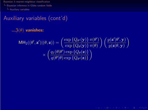
...Z(θ) vanishes:
MH2((θ′, z′)|(θ, z)) =
(exp {Qθ′(y)}π(θ′)
exp {Qθ(y)}π(θ)
) (g(z′|θ′,y)
g(z|θ,y)
)
×
(q1(θ|θ
′) exp {Qθ(z)}
q(θ′|θ) exp {Qθ′(z)}
)
Bayesian k-nearest-neighbour classification
Bayesian inference in Gibbs random fields
Auxiliary variables
Auxiliary variables (cont’d)
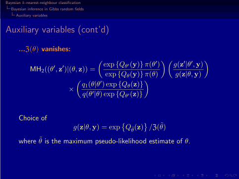
...Z(θ) vanishes:
MH2((θ′, z′)|(θ, z)) =
(exp {Qθ′(y)}π(θ′)
exp {Qθ(y)}π(θ)
) (g(z′|θ′,y)
g(z|θ,y)
)
×
(q1(θ|θ
′) exp {Qθ(z)}
q(θ′|θ) exp {Qθ′(z)}
)
Choice ofg(z|θ,y) = exp
{Q
θ(z)
}/Z(θ)
where θ is the maximum pseudo-likelihood estimate of θ.

Bayesian k-nearest-neighbour classification
Bayesian inference in Gibbs random fields
Auxiliary variables
Auxiliary variables (cont’d)
...Z(θ) vanishes:
MH2((θ′, z′)|(θ, z)) =
(exp {Qθ′(y)}π(θ′)
exp {Qθ(y)}π(θ)
) (g(z′|θ′,y)
g(z|θ,y)
)
×
(q1(θ|θ
′) exp {Qθ(z)}
q(θ′|θ) exp {Qθ′(z)}
)
Choice ofg(z|θ,y) = exp
{Q
θ(z)
}/Z(θ)
where θ is the maximum pseudo-likelihood estimate of θ.
New problem: Need to simulate from f(y|θ)
Bayesian k-nearest-neighbour classification
Perfect sampling
Perfect sampling
Coupling From The Past:algorithm that allows for exact and iid sampling from a givendistribution while using basic steps from an MCMC algorithm
Bayesian k-nearest-neighbour classification
Perfect sampling
Perfect sampling
Coupling From The Past:algorithm that allows for exact and iid sampling from a givendistribution while using basic steps from an MCMC algorithm
Underlying concept: run coupled Markov chains that start from allpossible states in the state space. Once all chains havemet/coalesced, they stick to the same path; the effect of the initialstate has “vanished”.
[Propp & Wilson, 1996]

Bayesian k-nearest-neighbour classification
Perfect sampling
Implementation for Potts (3)
In the case of a two-colour Ising model, existence of a perfectsampler by virtue of monotonicity properties: Potts
Bayesian k-nearest-neighbour classification
Perfect sampling
Implementation for Potts (3)
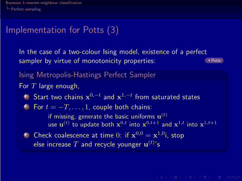
In the case of a two-colour Ising model, existence of a perfectsampler by virtue of monotonicity properties: Potts
Ising Metropolis-Hastings Perfect Sampler
For T large enough,
1 Start two chains x0,−t and x1,−t from saturated states2 For t = −T, . . . , 1, couple both chains:
if missing, generate the basic uniforms u(t)
use u(t) to update both x0,t into x0,t+1 and x1,t into x1,t+1
3 Check coalescence at time 0: if x0,0 = x1,0i, stopelse increase T and recycle younger u(t)’s

Bayesian k-nearest-neighbour classification
Perfect sampling
Implementation for Potts (3)
In the case of a two-colour Ising model, existence of a perfectsampler by virtue of monotonicity properties: Potts
Ising Metropolis-Hastings Perfect Sampler
For T large enough,
1 Start two chains x0,−t and x1,−t from saturated states2 For t = −T, . . . , 1, couple both chains:
if missing, generate the basic uniforms u(t)
use u(t) to update both x0,t into x0,t+1 and x1,t into x1,t+1
3 Check coalescence at time 0: if x0,0 = x1,0i, stopelse increase T and recycle younger u(t)’s
Limitation: Slow down & down when θ increase

Bayesian k-nearest-neighbour classification
k-nearest-neighbours
KNN’s as a probability distribution
1 MRFs
2 Bayesian inference in Gibbs random fields
3 Perfect sampling
4 k-nearest-neighboursKNN’s as a clustering ruleKNN’s as a probabilistic modelBayesian inference on KNN’sMCMC implementation
5 Pseudo-likelihood reassessed
Variable selection
Bayesian k-nearest-neighbour classification
k-nearest-neighbours
KNN’s as a clustering rule
KNN’s as a clustering rule
The k-nearest-neighbour procedure is a supervised clusteringmethod that allocates [new] subjects to one of G categories basedon the most frequent class [within a learning sample] in theirneighbourhood.

Bayesian k-nearest-neighbour classification
k-nearest-neighbours
KNN’s as a clustering rule
Supervised classification
Infer from a partitioned datasetthe classes of a new dataset

Bayesian k-nearest-neighbour classification
k-nearest-neighbours
KNN’s as a clustering rule
Supervised classification
Infer from a partitioned datasetthe classes of a new datasetData: training dataset
(ytr
i , xtri
)i=1,...,n
with class label 1 ≤ ytri ≤ Q and
predictor covariates xtri

Bayesian k-nearest-neighbour classification
k-nearest-neighbours
KNN’s as a clustering rule
Supervised classification
Infer from a partitioned datasetthe classes of a new datasetData: training dataset
(ytr
i , xtri
)i=1,...,n
with class label 1 ≤ ytri ≤ Q and
predictor covariates xtri
and testing dataset
(yte
i , xtei
)i=1,...,m
with unknown ytei ’s
−1.0 −0.5 0.0 0.5 1.0
−1
.0−
0.5
0.0
0.5
1.0
x2

Bayesian k-nearest-neighbour classification
k-nearest-neighbours
KNN’s as a clustering rule
Classification
Skip animation
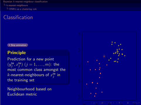
Principle
Prediction for a new point(yte
j , xtej ) (j = 1, . . . , m): the
most common class amongst thek-nearest-neighbours of xte
j inthe training set
Neighbourhood based onEuclidean metric
−1.0 −0.5 0.0 0.5 1.0
−1
.0−
0.5
0.0
0.5
1.0
x2
Bayesian k-nearest-neighbour classification
k-nearest-neighbours
KNN’s as a clustering rule
Classification
Skip animation
Principle
Prediction for a new point(yte
j , xtej ) (j = 1, . . . , m): the
most common class amongst thek-nearest-neighbours of xte
j inthe training set
Neighbourhood based onEuclidean metric
−1.0 −0.5 0.0 0.5 1.0
−1
.0−
0.5
0.0
0.5
1.0
x2
Bayesian k-nearest-neighbour classification
k-nearest-neighbours
KNN’s as a clustering rule
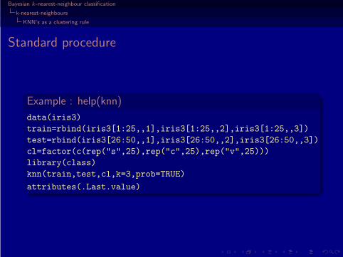
Standard procedure
Example : help(knn)
data(iris3)
train=rbind(iris3[1:25,,1],iris3[1:25,,2],iris3[1:25,,3])
test=rbind(iris3[26:50,,1],iris3[26:50,,2],iris3[26:50,,3])
cl=factor(c(rep("s",25),rep("c",25),rep("v",25)))
library(class)
knn(train,test,cl,k=3,prob=TRUE)
attributes(.Last.value)
Bayesian k-nearest-neighbour classification
k-nearest-neighbours
KNN’s as a clustering rule
Model choice perspective
Back to idea
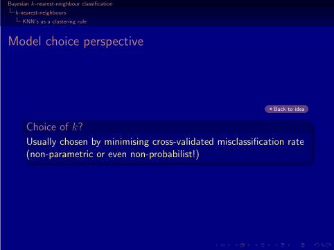
Choice of k?
Usually chosen by minimising cross-validated misclassification rate(non-parametric or even non-probabilist!)

Bayesian k-nearest-neighbour classification
k-nearest-neighbours
KNN’s as a clustering rule
Influence of k
Dataset of Ripley (1994),with two classes whereeach population of xi’s isfrom a mixture of twobivariate normaldistributions.Training set of n = 250points and testing set on aset of m = 1, 000 points
−1.0 −0.5 0.0 0.5 1.0
−0.
20.
00.
20.
40.
60.
81.
01.
2
k=1
−1.0 −0.5 0.0 0.5 1.0
−0.
20.
00.
20.
40.
60.
81.
01.
2
k=11
−1.0 −0.5 0.0 0.5 1.0
−0.
20.
00.
20.
40.
60.
81.
01.
2
k=57
−1.0 −0.5 0.0 0.5 1.0
−0.
20.
00.
20.
40.
60.
81.
01.
2
k=137
Bayesian k-nearest-neighbour classification
k-nearest-neighbours
KNN’s as a clustering rule
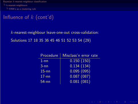
Influence of k (cont’d)
k-nearest-neighbour leave-one-out cross-validation:
Solutions 17 18 35 36 45 46 51 52 53 54 (29)
Procedure Misclass’n error rate
1-nn 0.150 (150)3-nn 0.134 (134)15-nn 0.095 (095)17-nn 0.087 (087)54-nn 0.081 (081)
Bayesian k-nearest-neighbour classification
k-nearest-neighbours
KNN’s as a probabilistic model
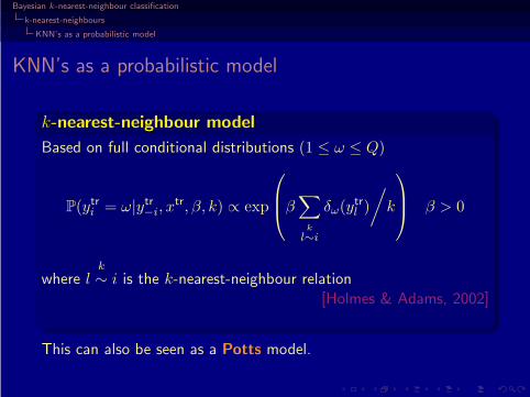
KNN’s as a probabilistic model
k-nearest-neighbour model
Based on full conditional distributions (1 ≤ ω ≤ Q)
P(ytri = ω|ytr
−i, xtr, β, k) ∝ exp
β∑
k
l∼i
δω(ytrl )
/k
β > 0
wherek
l ∼ i is the k-nearest-neighbour relation[Holmes & Adams, 2002]
This can also be seen as a Potts model.

Bayesian k-nearest-neighbour classification
k-nearest-neighbours
KNN’s as a probabilistic model
Motivations
β does not exist in the original k-nn procedure.

Bayesian k-nearest-neighbour classification
k-nearest-neighbours
KNN’s as a probabilistic model
Motivations
β does not exist in the original k-nn procedure.
It is only relevant from a statistical point of view as a measure ofuncertainty about the model:
β = 0 corresponds to a uniform distribution on all classes ;
β = +∞ leads to a point mass distribution on the prevalentclass.

Bayesian k-nearest-neighbour classification
k-nearest-neighbours
KNN’s as a probabilistic model
MRF-like expression
Closed form expression for the full conditionals
P(ytri = ω|ytr
−i, xtr, β, k) = exp (βnω(i)/k)
/ ∑
q
exp (βnq(i)/k)
where nω(i) number of neighbours of i with class label ω
Potts

Bayesian k-nearest-neighbour classification
k-nearest-neighbours
KNN’s as a probabilistic model
Drawback
Because the neighbourhoodstructure is not symmetric (xi
may be one of the k nearestneighbours of xj while xj is notone of the k nearest neighboursof xi),

Bayesian k-nearest-neighbour classification
k-nearest-neighbours
KNN’s as a probabilistic model
Drawback
Because the neighbourhoodstructure is not symmetric (xi
may be one of the k nearestneighbours of xj while xj is notone of the k nearest neighboursof xi), there usually is no jointprobability distributioncorresponding to these “fullconditionals”!
Bayesian k-nearest-neighbour classification
k-nearest-neighbours
KNN’s as a probabilistic model
Drawback (2)
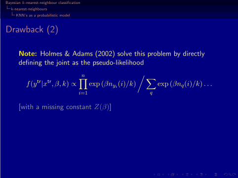
Note: Holmes & Adams (2002) solve this problem by directlydefining the joint as the pseudo-likelihood
f(ytr|xtr, β, k) ∝n∏
i=1
exp (βnyi(i)/k)
/ ∑
q
exp (βnq(i)/k) . . .
[with a missing constant Z(β)]

Bayesian k-nearest-neighbour classification
k-nearest-neighbours
KNN’s as a probabilistic model
Drawback (2)
Note: Holmes & Adams (2002) solve this problem by directlydefining the joint as the pseudo-likelihood
f(ytr|xtr, β, k) ∝n∏
i=1
exp (βnyi(i)/k)
/ ∑
q
exp (βnq(i)/k) . . .
[with a missing constant Z(β)]... but they are still using the same [wrong] predictive
P(ytej = ω|ytr, xtr, xte
j , β, k) = exp (βnω(j)/k)
/ ∑
q
exp (βnq(j)/k)

Bayesian k-nearest-neighbour classification
k-nearest-neighbours
KNN’s as a probabilistic model
Resolution
Symmetrise the neighbourhood relation:

Bayesian k-nearest-neighbour classification
k-nearest-neighbours
KNN’s as a probabilistic model
Resolution
Symmetrise the neighbourhood relation:
Principle: if xtri belongs to the
k-nearest-neighbour set for xtrj
and xtrj does not belong to the
k-nearest-neighbour set for xtri ,
xtrj is added to the set of
neighbours of xtri
Bayesian k-nearest-neighbour classification
k-nearest-neighbours
KNN’s as a probabilistic model
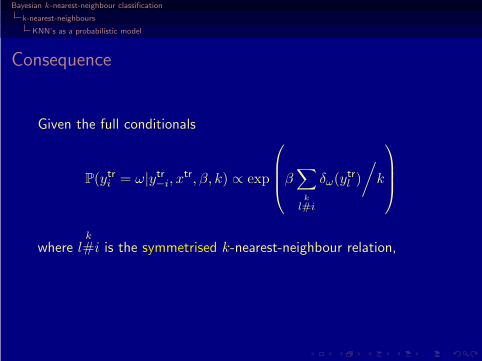
Consequence
Given the full conditionals
P(ytri = ω|ytr
−i, xtr, β, k) ∝ exp
β∑
k
l#i
δω(ytrl )
/k
wherek
l#i is the symmetrised k-nearest-neighbour relation,

Bayesian k-nearest-neighbour classification
k-nearest-neighbours
KNN’s as a probabilistic model
Consequence
Given the full conditionals
P(ytri = ω|ytr
−i, xtr, β, k) ∝ exp
β∑
k
l#i
δω(ytrl )
/k
wherek
l#i is the symmetrised k-nearest-neighbour relation,
there exists a corresponding joint distribution

Bayesian k-nearest-neighbour classification
k-nearest-neighbours
KNN’s as a probabilistic model
Extension to unclassified points
Predictive distribution of ytej (j = 1, . . . , m) defined as
P(ytej = ω|xte
j , ytr, xtr, β, k) ∝ exp
β∑
k
l#j
δω(ytrl )
/k
wherek
l#j is the symmetrised k-nearest-neighbour relation wrt thetraining set {xtr
1 , . . . , xtrn}
Bayesian k-nearest-neighbour classification
k-nearest-neighbours
Bayesian inference on KNN’s
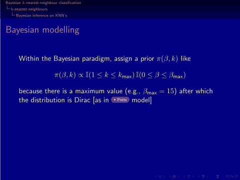
Bayesian modelling
Within the Bayesian paradigm, assign a prior π(β, k) like
π(β, k) ∝ I(1 ≤ k ≤ kmax) I(0 ≤ β ≤ βmax)
because there is a maximum value (e.g., βmax = 15) after whichthe distribution is Dirac [as in Potts model]
Bayesian k-nearest-neighbour classification
k-nearest-neighbours
Bayesian inference on KNN’s
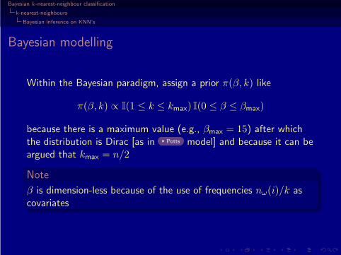
Bayesian modelling
Within the Bayesian paradigm, assign a prior π(β, k) like
π(β, k) ∝ I(1 ≤ k ≤ kmax) I(0 ≤ β ≤ βmax)
because there is a maximum value (e.g., βmax = 15) after whichthe distribution is Dirac [as in Potts model] and because it can beargued that kmax = n/2
Note
β is dimension-less because of the use of frequencies nω(i)/k ascovariates

Bayesian k-nearest-neighbour classification
k-nearest-neighbours
Bayesian inference on KNN’s
Bayesian global inference
Use marginal predictive distribution of ytej given xte
j (j = 1, . . . , m)
∫P(yte
j = ω|xtej , ytr, xtr, β, k)π(β, k|ytr, xtr)dβ dk
whereπ(β, k|ytr, xtr) ∝ f(ytr|xtr, β, k)π(β, k)
posterior distribution of (β, k) given the training dataset ytr
[ytej = MAP estimate]
Note
Model choice with no varying dimension because β is the same forall models
Bayesian k-nearest-neighbour classification
k-nearest-neighbours
MCMC implementation
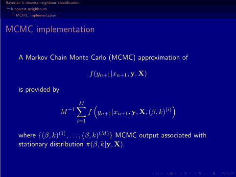
MCMC implementation
A Markov Chain Monte Carlo (MCMC) approximation of
f(yn+1|xn+1,y,X)
is provided by
M−1M∑
i=1
f(yn+1|xn+1,y,X, (β, k)(i)
)
where {(β, k)(1), . . . , (β, k)(M)} MCMC output associated withstationary distribution π(β, k|y,X).
Bayesian k-nearest-neighbour classification
k-nearest-neighbours
MCMC implementation
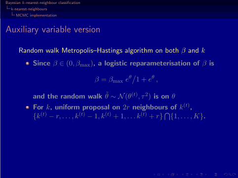
Auxiliary variable version
Random walk Metropolis–Hastings algorithm on both β and k
Since β ∈ (0, βmax), a logistic reparameterisation of β is
β = βmax eθ/1 + eθ ,
and the random walk θ ∼ N (θ(t), τ2) is on θ
For k, uniform proposal on 2r neighbours of k(t),{k(t) − r, . . . , k(t) − 1, k(t) + 1, . . . k(t) + r}
⋂{1, . . . , K}.

Bayesian k-nearest-neighbour classification
k-nearest-neighbours
MCMC implementation
Auxiliary variable version
Random walk Metropolis–Hastings algorithm on both β and k
Since β ∈ (0, βmax), a logistic reparameterisation of β is
β = βmax eθ/1 + eθ ,
and the random walk θ ∼ N (θ(t), τ2) is on θ
For k, uniform proposal on 2r neighbours of k(t),{k(t) − r, . . . , k(t) − 1, k(t) + 1, . . . k(t) + r}
⋂{1, . . . , K}.
Simulation of f(ztr|xtr, β, k) by perfect sampling taking advantageof monotonicity properties [but may get stuck for too large valuesof β]
Bayesian k-nearest-neighbour classification
k-nearest-neighbours
MCMC implementation
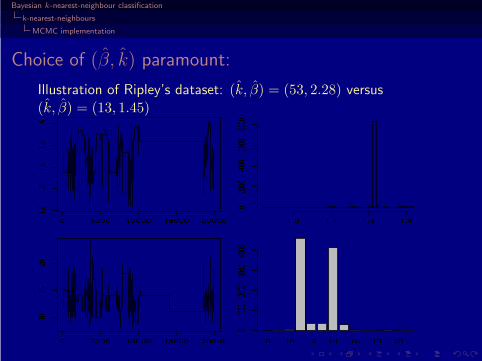
Choice of (β, k) paramount:
Illustration of Ripley’s dataset: (k, β) = (53, 2.28) versus(k, β) = (13, 1.45)

Bayesian k-nearest-neighbour classification
k-nearest-neighbours
MCMC implementation
Choice of (β, k) paramount:
Illustration of Ripley’s dataset: (k, β) = (53, 2.28) versus(k, β) = (13, 1.45)

Bayesian k-nearest-neighbour classification
k-nearest-neighbours
MCMC implementation
Diabetes in Pima Indian women
Example (R benchmark)
“A population of women who were at least 21 years old, of Pima Indianheritage and living near Phoenix (AZ), was tested for diabetes accordingto WHO criteria. The data were collected by the US National Institute ofDiabetes and Digestive and Kidney Diseases. We used the 532 completerecords after dropping the (mainly missing) data on serum insulin.”
number of pregnancies
plasma glucose concentration in an oral glucose tolerance test
diastolic blood pressure
triceps skin fold thickness
body mass index
diabetes pedigree function
age

Bayesian k-nearest-neighbour classification
k-nearest-neighbours
MCMC implementation
Diabetes in Pima Indian womenMCMC output for βmax = 1.5, β = 1.15, k = 40, and 20, 000simulations.
Bayesian k-nearest-neighbour classification
k-nearest-neighbours
MCMC implementation
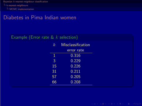
Diabetes in Pima Indian women
Example (Error rate & k selection)
k Misclassificationerror rate
1 0.3163 0.22915 0.22631 0.21157 0.20566 0.208

Bayesian k-nearest-neighbour classification
k-nearest-neighbours
MCMC implementation
Predictive output
The approximate Bayesian prediction of yn+1 is
yn+1 = arg maxg
M−1M∑
i=1
f(g|xn+1,y,X, β(i), k(i)
).

Bayesian k-nearest-neighbour classification
k-nearest-neighbours
MCMC implementation
Predictive output
The approximate Bayesian prediction of yn+1 is
yn+1 = arg maxg
M−1M∑
i=1
f(g|xn+1,y,X, β(i), k(i)
).
E.g., Ripley’s dataset misclassification error rate: 0.082.

Bayesian k-nearest-neighbour classification
Pseudo-likelihood reassessed
A reassessment of pseudo-likelihood
1 MRFs
2 Bayesian inference in Gibbs random fields
3 Perfect sampling
4 k-nearest-neighbours
5 Pseudo-likelihood reassessed
6 Variable selection
Bayesian k-nearest-neighbour classification
Pseudo-likelihood reassessed
Pseudo-likelihood
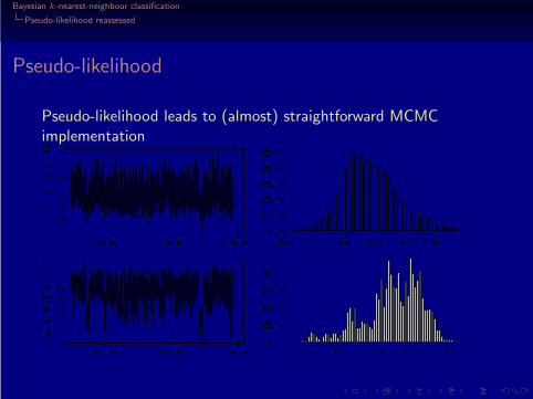
Pseudo-likelihood leads to (almost) straightforward MCMCimplementation

Bayesian k-nearest-neighbour classification
Pseudo-likelihood reassessed
Magnitude of the approximation
Since perfect and path sampling approaches also are available forsmall datasets, possibility of evaluation of pseudo-likelihoodapproximation

Bayesian k-nearest-neighbour classification
Pseudo-likelihood reassessed
Ripley’s benchmark (1)
Approximations to the posterior of β based on the pseudo (green),the path (red) and the perfect (yellow) schemes withk = 1, 10, 70, 125, for 20, 000 iterations:

Bayesian k-nearest-neighbour classification
Pseudo-likelihood reassessed
Ripley’s benchmark (2)
Approximations of posteriors of β (top) and k (bottom)

Bayesian k-nearest-neighbour classification
Variable selection
Variable selection
1 MRFs
2 Bayesian inference in Gibbs random fields
3 Perfect sampling
4 k-nearest-neighbours
5 Pseudo-likelihood reassessed
6 Variable selection
Bayesian k-nearest-neighbour classification
Variable selection
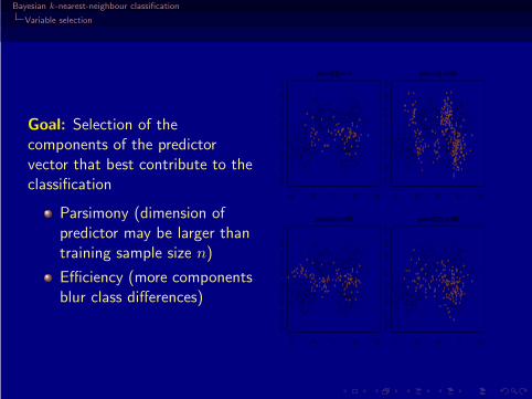
Goal: Selection of thecomponents of the predictorvector that best contribute to theclassification
Parsimony (dimension ofpredictor may be larger thantraining sample size n)
Efficiency (more componentsblur class differences)
−1.0 −0.5 0.0 0.5 1.0
−0
.20
.00
.20
.40
.60
.81
.01
.2
gamma=(1,1), err=78
−1.0 −0.5 0.0 0.5 1.0
−0
.20
.00
.20
.40
.60
.81
.01
.2
gamma=(1,0), err=284
−1.0 −0.5 0.0 0.5 1.0
−0
.20
.00
.20
.40
.60
.81
.01
.2
gamma=(0,1), err=116
−1.0 −0.5 0.0 0.5 1.0
−0
.20
.00
.20
.40
.60
.81
.01
.2
gamma=(1,1,1), err=159
Bayesian k-nearest-neighbour classification
Variable selection
Component indicators
Completion of (β, k) with indicator variables γj ∈ {0, 1}(1 ≤ j ≤ p) that determine which components of x are active inthe model
P(yi = Cj |y−i,X, β, k,γ) ∝ exp
β∑
l∈vk(i)
δCj(yl)
/k
with vk(i) (symmetrised) k nearest neighbourhood of xi for thedistance
d(xi, xℓ)2 =
p∑
j=1
γj(xij − xℓj)2
Bayesian k-nearest-neighbour classification
Variable selection
Variable selection
Formal similarity with usual variable selection in regression models.Use of a uniform prior on the γj ’s on {0, 1}, independently for allj’sExploration of a range of models Mγ of size 2p that may be toolarge (see, e.g., the vision dataset with p = 200)
Bayesian k-nearest-neighbour classification
Variable selection
Implementation
Use of a naive “reversible jump” MCMC, where
1 (β, k) are changed conditional on γ and
2 γ is changed one component at a time conditional on (β, k)[and the data]
Note
Validation of simple jumps due to (a) saturation of the dimensionby associating a γj to each variable and (b) hierarchical structureof the (β, k) part.
c© This is not a varying dimension problem
Bayesian k-nearest-neighbour classification
Variable selection
MCMC algorithm
Variable selection k-nearest-neighbours
At time 0, generate γ(0)j ∼ B(1/2), log β(0) ∼ N
(0, τ2
)and
k(0) ∼ U{1,...,K}
At time 1 ≤ t ≤ T ,
1 Generate log β ∼ N(log β(t−1), τ2
)and
k ∼ U ({k − r, k − r + 1, . . . , k + r − 1, k + r})
2 Calculate Metropolis-Hastings acceptance probabilityρ(β, k, β(t−1), k(t−1))
3 Move to(β(t), k(t)
)by Metropolis-Hastings step
4 For j = 1, . . . , p, generate γ(t)j ∼ π(γj |y,X, γ
(t)−j , β
(t), k(t))
Bayesian k-nearest-neighbour classification
Variable selection
Benchmark 1
Ripley’s dataset with 8 additional potential [useless] covariatessimulated from N (0, .052)
Using the 250 datapoints for variable selection, comparison of the210 = 1024 models by pseudo-maximum likelihood estimation of(k, β) and by comparison of pseudo-likelihoods leads to select theproper submodel
γ1 = γ2 = 1 and γ3 = · · · = γ10 = 0
with k = 3.1 and β = 3.8. Forward and backward selectionprocedures lead to same conclusion.
MCMC algorithm produces γ1 = γ2 = 1 and γ3 = · · · = γ10 = 0 asthe MMAP, with very similar values for k and β [Hardly any moveaway from (1, 1, 0, . . . , 0) is accepted]

Bayesian k-nearest-neighbour classification
Variable selection
Benchmark 2
Ripley’s dataset with now 28 additional covariates simulated fromN (0, .052)
Using the 250 datapoints for variable selection, direct comparisonof the 230 models by pseudo-maximum likelihood estimationimpossible!
Forward and backward selection procedures both lead to the propersubmodel γ = (1, 1, 0, . . . , 0)

Bayesian k-nearest-neighbour classification
Variable selection
Benchmark 2
Ripley’s dataset with now 28 additional covariates simulated fromN (0, .052)
Using the 250 datapoints for variable selection, direct comparisonof the 230 models by pseudo-maximum likelihood estimationimpossible!
Forward and backward selection procedures both lead to the propersubmodel γ = (1, 1, 0, . . . , 0)MCMC algorithm again produces γ1 = γ2 = 1 andγ3 = · · · = γ10 = 0 as the MMAP, with more moves aroundγ = (1, 1, 0, . . . , 0)