Bayesian inference and mathematical imaging. Part III ...

Bayesian inference and mathematical imaging.Part III: probability & convex optimisation.

Dr. Marcelo Pereyrahttp://www.macs.hw.ac.uk/∼mp71/

Maxwell Institute for Mathematical Sciences, Heriot-Watt University

January 2019, CIRM, Marseille.

M. Pereyra (MI — HWU) Bayesian mathematical imaging 0 / 53

Outline

1 Bayesian inference in imaging inverse problems

2 MAP estimation with Bayesian confidence regionsPosterior credible regionsUncertainty visualisationHypothesis testing

3 A decision-theoretic derivation of MAP estimation

4 Hierarchical MAP estimation with unknown regularisation parameters

5 Conclusion


Imaging inverse problems

We are interested in an unknown image x ∈ Rd .

We measure y , related to x by a statistical model p(y ∣x).

The recovery of x from y is ill-posed or ill-conditioned, resulting insignificant uncertainty about x .

For example, in many imaging problems

y = Ax +w ,

for some operator A that is rank-deficient, and additive noise w .


The Bayesian framework

We use priors to reduce uncertainty and deliver accurate results.

Given the prior p(x), the posterior distribution of x given y

p(x ∣y) = p(y ∣x)p(x)/p(y)

models our knowledge about x after observing y .

In this talk we consider that p(x ∣y) is log-concave; i.e.,

p(x ∣y) = exp{−φ(x)}/Z ,

where φ(x) is a convex function and Z = ∫ exp{−φ(x)}dx .


Maximum-a-posteriori (MAP) estimation

The predominant Bayesian approach in imaging is MAP estimation

xMAP = argmaxx∈Rd

p(x ∣y),

= argminx∈Rd

φ(x),(1)

computed efficiently, even in very high dimensions, by (proximal) convexoptimisation (Green et al., 2015; Chambolle and Pock, 2016).

However, MAP estimation has some limitations, e.g.,

1 it provides little information about p(x ∣y),

2 it is not theoretically well understood (yet),

3 it struggles with unknown/partially unknown models.


Illustrative example: astronomical image reconstruction

Recover x ∈ Rd from low-dimensional degraded observation

y =MFx +w ,

where F is the continuous Fourier transform, M ∈ Cm×d is a measurementmask operator, and w is Gaussian noise. We use the model

p(x ∣y)∝ exp (−∥y −MFx∥2/2σ2

− θ∥Ψx∥1)1Rn+(x). (2)

∣y ∣xMAP

Figure : Radio-interferometric image reconstruction of the W28 supernova.M. Pereyra (MI — HWU) Bayesian mathematical imaging 5 / 53

Outline





5 Conclusion


Posterior credible regions

Where does the posterior probability mass of x lie?

Recall that Cα is a (1 − α)% posterior credible region if

P [x ∈ Cα∣y] = 1 − α,

and the decision-theoretically optimum is the HPD region (Robert, 2001)

C∗α = {x ∶ φ(x) ≤ γα} ,

with γα ∈ R chosen such that ∫C∗αp(x ∣y)dx = 1 − α holds.

We could estimate C∗α by MCMC sampling, but in high-dimensional

log-concave models this is not necessary because something beautifulhappens...


A concentration phenomenon!

Figure : Convergence to “typical” set {x ∶ log p(x ∣y) ≈ E[log p(x ∣y)]}.


Proposed approximation of C ∗α

Theorem 2.1 (Pereyra (2016))

Suppose that the posterior p(x ∣y) = exp{−φ(x)}/Z is log-concave on Rd .Then, for any α ∈ (4 exp (−n/3),1), the HPD region C∗

α is contained by

Cα = {x ∶ φ(x) ≤ φ(xMAP) +√dτα + d)},

with universal positive constant τα =√

16 log(3/α) independent of p(x ∣y).

Remark 1: Cα is a conservative approximation of C∗α , i.e.,

x ∉ Cα Ô⇒ x ∉ C∗α .

Remark 2: Cα is available as a by-product in any convex inferenceproblem that is solved by MAP estimation!


Approximation error bounds

Is Cα a reliable approximation of C∗α?

Theorem 2.2 (Finite-dimensional error bound (Pereyra, 2016))

Let γα = φ(xMAP) +√dτα + d . If p(x ∣y) is log-concave on Rd , then

0 ≤γα − γα

d≤ 1 + ηαd

−1/2,

with universal positive constant ηα =√

16 log(3/α) +√

1/α.

Remark 3: Cα is stable (as d becomes large, the error (γα − γα)/d ⪅ 1).Remark 4: The lower and upper bounds are asymptotically tight w.r.t. d .


Outline





5 Conclusion


Example: Uncertainty visualisation in astro-imaging

Radio-interferometry with redundant wavelet frame (Cai et al., 2017).

dirty image xpenML(y) xMAP

approx. credible intervals (scale 10 × 10 pixels) “exact” intervals (MCMC, minutes)

M31 radio galaxy (size 256 × 256 pixels, comp. time 1.8 secs.)


Example: Uncertainty visualisation in astro-imaging

Radio-interferometry with redundant wavelet frame (Cai et al., 2017).

dirty image xpenML(y) xMAP

approx. credible intervals (scale 10 × 10 pixels) “exact” intervals (MCMC, minutes)

3C2888 radio galaxy (size 256 × 256 pixels, comp. time 1.8 secs.)


Example: uncertainty visualisation in microscopy

Live cell microscopy sparse super-resolution (Zhu et al., 2012):

y = Ax +w(A is a blur operator)

xMAP = argminx∈Rd ∥y−Hx∥2/2σ2+λ∥x∥1

(log-scale)

Consider the molecular structure in the highlighted region:

Are we confident about this structure (its presence, position, etc.)?

Idea: use Cα to explore/quantify the uncertainty about this structure.


Example: uncertainty visualisation in microscopy

Position uncertainty quantificationFind maximum molecule displacement within C0.05:

xMAP = argminx∈Rd ∥y−Ax∥2/2σ2+λ∥x∥1Molecule position uncertainty

(±93nm × ±140nm)

Note: Uncertainty analysis (±93nm × ±140nm) in agreement with MCMCestimates (±78nm × ±125nm - approx. error of order of 1 pixel), and withexperimental results (average precision ±80nm) of Zhu et al. (2012).


Outline





5 Conclusion


Hypothesis testing

Bayesian hypothesis test for specific image structures (e.g., lesions)

H0 ∶ The structure of interest is ABSENT in the true image

H1 ∶ The structure of interest is PRESENT in the true image

The null hypothesis H0 is rejected with significance α if

P(H0∣y) ≤ α.

Theorem (Repetti et al., 2018)Let S denote the region of Rd associated with H0, containing all imageswithout the structure of interest. Then

S ∩ Cα = ∅ Ô⇒ P(H0∣y) ≤ α .

If in addition S is convex, then checking S ∩ Cα = ∅ is a convex problem

minx , x∈Rd

∥x − x∥22 s.t. x ∈ Cα , x ∈ S .


Uncertainty quantification in MRI imaging

xMAP x ∈ C0.01 x ∈ S

xMAP (zoom) x ∈ C0.01 (zoom) x ∈ S (zoom)

MRI experiment: test images x = x, hence we fail to reject H0 and conclude that

there is little evidence to support the observed structure.


Uncertainty quantification in MRI imaging

xMAP x ∈ C0.01 x ∈ S0

xMAP (zoom) x ∈ C0.01 (zoom) x ∈ S0 (zoom)

MRI experiment: test images x ≠ x, hence we reject H0 and conclude that there is

significant evidence in favour of the observed structure.


Uncertainty quantification in radio-interferometric imaging

Quantification of minimum energy of different energy structures, at level(1 − α) = 0.99, as the number of measurements T = dim(y)/2 increases.

∣y ∣ xMAP(T = 200)ρα, energy ratio preserved at α = 0.01

Figure : Analysis of 3 structures in the W28 supernova RI image.

Note: energy ratio calculated as

ρα =∥x − x∥2

∥xMAP − xMAP∥2

where x , x are computed with α = 0.01, and xMAP is a modified version of xMAP

where the structure of interest has been carefully removed from the image.M. Pereyra (MI — HWU) Bayesian mathematical imaging 21 / 53

Outline





5 Conclusion


Bayesian point estimators

Bayesian point estimators arise from the decision ”what point x ∈ Rd

summarises x ∣y best?”. The optimal decision under uncertainty is

xL = argminu∈Rd

E{L(u, x)∣y} = argminu∈Rd

∫ L(u, x)p(x ∣y)dx

where the loss L(u, x) measures the “dissimilarity” between u and x .

Example: Euclidean setting L(u, x) = ∥u − x∥2 and xL = xMMSE = E{x ∣y}.

General desiderata:

1 L(u, x) ≥ 0, ∀u, x ∈ Rd ,

2 L(u, x) = 0 ⇐⇒ u = x ,

3 L strictly convex w.r.t. its first argument (for estimator uniqueness).


Bayesian point estimators

Does the convex geometry of p(x ∣y) define an interesting loss L(u, x)?

We use differential geometry to relate the convexity of p(x ∣y), thegeometry of the parameter space, and the loss L to perform estimation.


Differential geometry

A Riemannian manifold M = (Rd ,g), with metric g ∶ Rd → Sd++ and globalcoordinate system x , is a vector space that is locally Euclidean.

For any point x ∈ Rd we have an Euclidean tangent space TxRd with innerproduct ⟨u, x⟩ = u⊺g(x)x and norm ∥x∥ =

√x⊺g(x)x .

This geometry is local and may vary smoothly from TxRd to Tx ′Rd

following the affine connection Γ ∈ Rd×d×d , given by Γij , k(x) = ∂kgi ,j(x).


Divergence functions

Similarly to Euclidean spaces, the manifold (Rd ,g) supports divergences:

Definition 1 (Divergence functions)

A function D ∶ Rd ×Rd → R is a divergence function on Rd if the followingconditions hold for any u, x ∈ Rd :

D(u, x) ≥ 0, ∀u, x ∈ Rd ,

D(u, x) = 0 ⇐⇒ x = u,

D(u, x) is strongly convex w.r.t. u, and C2 w.r.t u and x .


Canonical divergence

We focus on the canonical divergence on (Rd ,g), a generalisation of theEuclidean squared distance to this kind of manifold:

Definition 2 (Canonical divergence (Ay and Amari, 2015))

For any (u, x) ∈ Rd ×Rd , the canonical divergence on (Rd ,g) is given by

D(u, x) = ∫1

0tγt

⊺g(γt)γtdt (3)

where γt is the Γ-geodesic from u to x and γt = d/dt γt .

1 D fully species (Rd ,g) and vice-versa.

2 D(x + dx , x) = ∥dx∥2/2 + o(∥dx∥2) where ∥ ⋅ ∥ is the norm on TxRd .

3 For Euclidean space with ⟨u, x⟩ = u⊺gx , D(u, x) = 12(u − x)⊺g(u − x).


Differential-geometric derivation of xMAP and xMMSE

Theorem 3 (Canonical Bayesian estimators - Part 1 (Pereyra, 2016))

Suppose that φ(x) = − log p(x ∣y) is strongly convex, continuous, and C3

on Rd . Let (Rd ,g) be the manifold induced by φ, i.e., gi ,j(x) = ∂i∂jφ(x).Then, the canonical divergence on (Rd ,g) is the φ-Bregman divergence

Dφ(u, x) = φ(u) − φ(x) −∇φ(x)(u − x).

Remark: Because φ is strongly convex, then φ(u) > φ(x) −∇φ(x)(u − x)for any u ≠ x . The divergence Dφ(u, x) quantifies this gap, related to thelength of the affine geodesic from u to x on the space induced by p(x ∣y).




The Bayesian estimator associated with Dφ(u, x) is unique and is given by

xDφ ≜ argminu∈Rd

Ex ∣y [Dφ(u, x)] ,

= argminx∈Rd

φ(x) ,

= xMAP .

Remark2: xMAP stems from Bayesian decision theory, and hence it standson the same theoretical footing as the core Bayesian methodologies.

Remark3: The definition of the MAP estimator as the maximiserxMAP = argmaxx∈Rd p(x ∣y) is mainly algorithmic for these models.




Moreover, the Bayesian estimator associated with the dual canonicaldivergence D∗

φ(u, x) = Dφ(x ,u) is also unique and is given by

xD∗φ≜ argmin

u∈Rd

Ex ∣y [D∗φ(u, x)] ,

= ∫Rd

xp(x ∣y)dx ,

= xMMSE .

Remark 4: xMAP and xMMSE exhibit a surprising duality, arising from theasymmetry of the canonical divergence that p(x ∣y) induces on Rd .

Remark 5: These results carry partially to models that are not stronglyconvex, not smooth, or that involve constraints on the parameter space.


Expected estimation error bound

Are xMAP and xMMSE “good” estimators of x ∣y ?

Proposition 3.1 (Expected canonical error bound)

Suppose that φ(x) = − logπ(x ∣y) is convex on Rd and C1. Then,

Ex ∣y [D∗φ(xMMSE , x)/d] ≤ Ex ∣y [D∗

φ(xMAP , x)/d] ≤ 1.

Proposition 3.2 (Expected error w.r.t. regularisation function)

Also assume that the regularisation h(x) = − log p(x) is convex. Then,

Ex ∣y [D∗h (xMMSE , x)/d] ≤ Ex ∣y [D∗

h (xMAP , x)/d] ≤ 1.

Remark 6: These are high-dimensional stability results for xMAP andxMMSE ; the estimation error cannot grow faster than the number of pixels.


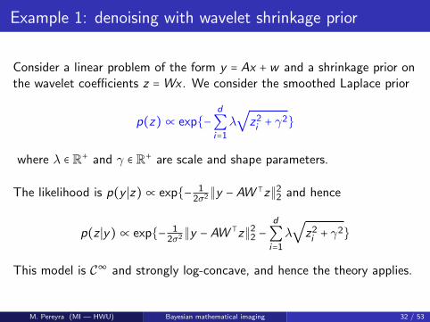
Example 1: denoising with wavelet shrinkage prior

Consider a linear problem of the form y = Ax +w and a shrinkage prior onthe wavelet coefficients z =Wx . We consider the smoothed Laplace prior

p(z)∝ exp{−d

∑i=1

λ√

z2i + γ

2}

where λ ∈ R+ and γ ∈ R+ are scale and shape parameters.

The likelihood is p(y ∣z)∝ exp{− 12σ2 ∥y −AW ⊺z∥2

2 and hence

p(z ∣y)∝ exp{− 12σ2 ∥y −AW ⊺z∥2

2 −d

∑i=1

λ√

z2i + γ

2}

This model is C∞ and strongly log-concave, and hence the theory applies.



To analyse the geometry induced by φ(z) = − log p(z ∣y) we suppose thatA = I and W ⊺W = I, and obtain Dφ(u, z) = ∑

di=1 Dψ(ui , zi) with

Dψ(ui , zi) =1

2σ2(ui − zi)

2+ λ

√z2i + γ

2√

u2i + γ

2 − ziui − γ2

√z2i + γ

2.

The non-quadratic term introduces additional shrinkage and leads to thedifferences between xMMSE and xMAP .

To develop an intuition for this behaviour we analyse zi ≪ γ and zi ≫ γ.



When zi ≫ γ the non-quadratic term vanishes, hence

Dψ(ui , zi) ≈1

2σ2 (ui − zi)2 .

Hence, when p(zi ∣y) has most of its mass in large values of zi , the MAPestimate for zi will agree with the MMSE estimate E(zi ∣y).

In this case there is no additional shrinkage from the estimator.



Conversely, when zi ≪ γ we have

Dψ(ui , zi) ≈1

2σ2 (ui − zi)2+ λ∣ui ∣ ,

≈ 12σ2 u

2i + λ∣ui ∣ ,

for ui ≫ γ, and for ui ≪ γ we obtain

Dψ(ui , zi) ≈1

2σ2 (ui − zi)2+ λ [

u2i

2γ+

z2i

2α−−ziuiγ

] = (1

2σ2+λ

2γ) (ui − zi)

22

In these two cases Dψ boosts the effect of the shrinkage prior by promotingui values that are close to zero (explicitly via the penalty λ∣ui ∣, or byamplifying the constant of the quadratic loss from 1/2σ2 to 1/2σ2 +λ/2γ).



Illustration with the Flinstones image (σ = 0.08, λ = 12 and γ = 0.01).

noisy image y (SNR 17.6dB) xMAP (SNR 19.8dB)

xMMSE (SNR 17.7dB) denoising functions for zMAP and zMMSE

Illustrative example of a model where the action of the shrinkage prior acts

predominantly via Dψ (Note: setting γ = 0 leads to xMAP with SNR 18.8dB).M. Pereyra (MI — HWU) Bayesian mathematical imaging 36 / 53

Illustrative example: astronomical image reconstruction

Generalisation warning: shrinkage priors can also act predominantly via themodel (not Dψ), producing similar xMAP and xMMSE results; e.g.,

dirty image xpenML(y) xMAP xMMSE

Radio-interferometric imaging of the Cygnus A galaxy ?.


Outline





5 Conclusion


Problem statement

We consider the class of priors of the form

p(x ∣θ) = exp{−θh(x)}/C(λ)

where h ∶ Rn → [0,∞] promotes expected properties of x , and θ ∈ R+ is a“regularisation” parameter controlling the strength of the prior.

When θ is fixed and the posterior p(x ∣y , θ) is log-concave,

x(θ)MAP = argmin

x∈Rd

gy(x) + θh(x)− logC(θ) − log p(y),

is a convex optimisation problem that can be often solved efficiently.

Here we consider the infamous problem of not specifying the value of θ.


Hierarchical Bayesian treatment of unknown θ

Hierarchical Bayesian inference allows estimating x without specifying θ.

We incorporate θ to the model by assigning it an hyper-prior p(θ).

The extended model is

p(x , θ∣y) = p(y ∣x)p(x ∣θ)p(θ)/p(y),

∝exp{−gy(x) − θh(x) − log p(θ)}

C(θ),

(4)

but C(θ) = ∫Rd exp{−θh(x)}dx is typically intractable!

If we had access to C(θ) we could either estimate x and θ jointly, oralternatively marginalise θ followed by inference on x .


Idea: Use Prox-MCMC to estimate E [h(x)∣θ] over a θ-grid, and thenapproximate logC(θ) by using the identity d

dθ logC(θ) = E [h(x)∣θ].

Figure : Monte Carlo approximations of E [h(x)∣θ] for 4 widely used priordistributions and for θ ∈ [10−3,102]. Surprise: they all coincide!


Main theoretical result

Definition 4.1 (k-homogeneity)

The regulariser h is a k-homogeneous function if ∃k ∈ R+ such that

h(ηx) = ηkh(x), ∀x ∈ Rd ,∀η > 0. (5)

Theorem 4.1 (Pereyra et al. (2015))

Suppose that h, the sufficient statistic of p(x ∣θ), is k-homogenous. Thenthe normalisation factor has the form

C(θ) = Dθ−d/k ,

with (generally intractable) constant D = C(1) independent of θ.

Note: This result holds for all norms (e.g., `1, `2, total-variation, nuclear,etc.), composite norms (e.g., `1 − `2), and compositions of norms withlinear operators (e.g., analysis terms of the form ∥Ψx∥1)!


Marginal maximum-a-posteriori estimation of x

Knowledge of C(λ) enables (for example) marginal MAP estimation of x

x†MAP = argmax

x∈Rd∫

∞

0p(x , λ∣y)dλ,

= argminx∈Rd

gy(x) + (d/k + α) log{h(x) + β},(6)

where we have used the hyper-prior λ ∼ Gamma(α,β).

We can compute x† efficiently by majorisation-minimisation optimisation

x(t) = argminx∈Rd

gy(x) + θ(t−1)h(x),

θ(t) =d/k + α

h(x(t)) + β.

(7)

which is also an expectation-maximisation algorithm.


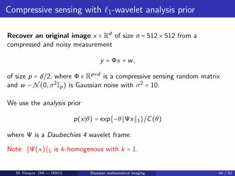
Compressive sensing with `1-wavelet analysis prior

Recover an original image x ∈ Rd of size n = 512 × 512 from acompressed and noisy measurement

y = Φx +w ,

of size p = d/2, where Φ ∈ Rp×d is a compressive sensing random matrixand w ∼ N (0, σ2Ip) is Gaussian noise with σ2 = 10.

We use the analysis prior

p(x ∣θ) = exp{−θ∥Ψx∥1}/C(θ)

where Ψ is a Daubechies 4 wavelet frame.

Note: ∥Ψ(x)∥1 is k-homogenous with k = 1.


Experiment with the Boat and Mandrill test images

(θ∗ = 56.4, PSNR=33.4) (θ∗ = 2.04, PSNR=25.3)

Figure : Compressive sensing experiment with the Boat and Mandrill testimages, with automatic selection of θ by marginalisation - see (7).


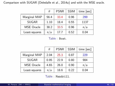
Comparison with SUGAR (Deledalle et al., 2014a) and with the MSE oracle.

θ PSNR SSIM time [sec]

Marginal MAP 56.4 33.4 0.96 299

SUGAR 1.10 18.4 0.55 1137

MSE Oracle 38.2 33.5 0.96 n/a

Least-squares n/a 17.7 0.52 0.04

Table : Boat.

θ PSNR SSIM time [sec]

Marginal MAP 2.04 25.3 0.87 229

SUGAR 0.95 22.9 0.80 984

MSE Oracle 4.65 26.0 0.90 n/a

Least-squares n/a 18.6 0.22 0.04

Table : Mandrill.


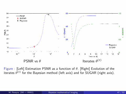
PSNR vs θ Iterates θ(t)

Figure : [Left] Estimation PSNR as a function of θ. [Right] Evolution of theiterates θ(t) for the Bayesian method (left axis) and for SUGAR (right axis).


Illustrative example - Image deblurring with TV prior

In a manner akin to Fernandez-Vidal and Pereyra (2018), we also applythe method to the Bayesian image deblurring model

p(x ∣y , θ)∝ exp (−∥y −Ax∥2/2σ2

− θ∥∇dx∥1−2) ,

and compute θ = argmaxθ∈R+ p(y ∣θ).

We obtain the following results:

Method SNR=20 dB SNR=30 dB SNR=40 dBAvg. MSE Avg. Time Avg. MSE Avg. Time Avg. MSE Avg. Time

θ∗(Oracle) 22.95 ± 3.10 – 21.05 ± 3.19 – 18.76 ± 3.19 –Marginalization 24.67 ± 3.08 17.27 22.39 ± 3.07 6.31 19.44 ± 3.26 6.77Empirical Bayes 23.24 ± 3.23 43.01 21.16 ± 3.24 41.50 18.90 ± 3.39 42.85

SUGAR 24.14 ±3.19 15.74 23.96 ± 3.26 20.87 23.94± 3.27 20.59

Comparison with the empirical Bayesian method (Fernandez-Vidal and Pereyra, 2018), the SUGAR method (Deledalle et al.,2014b), and an oracle that knows the optimal value of θ. Average values over 10 test images of size 512 × 512 pixels.

An exhaustive evaluation comparing different methods on a range of imagingproblems will be reported soon.


Outline





5 Conclusion


Conclusion

The challenges facing modern imaging sciences require amethodological paradigm shift to go beyond point estimation.

In Part I we discussed how the Bayesian framework can support thisparadigm shift, provided we significantly accelerate computations.

In Part II we considered efficiency improvements by integratingmodern stochastic and variational computation approaches.

In Part III we explored methods based on convex optimisation andprobability, and developed theory for MAP estimation.


Conclusion

In the next lecture...We will explore Bayesian models and stochastic computation algorithmsfor problems that are significantly more difficult, and where deterministicapproaches fail.

Thank you!


Bibliography:

Ay, N. and Amari, S.-I. (2015). A novel approach to canonical divergences withininformation geometry. Entropy, 17(12):7866.

Cai, X., Pereyra, M., and McEwen, J. D. (2017). Uncertainty quantification for radiointerferometric imaging II: MAP estimation. ArXiv e-prints.

Chambolle, A. and Pock, T. (2016). An introduction to continuous optimization forimaging. Acta Numerica, 25:161–319.

Deledalle, C., Vaiter, S., Peyre, G., and Fadili, J. (2014a). Stein Unbiased GrAdientestimator of the Risk (SUGAR) for multiple parameter selection. SIAM J. ImagingSci., 7(4):2448–2487.

Deledalle, C.-A., Vaiter, S., Fadili, J., and Peyre, G. (2014b). Stein unbiased gradientestimator of the risk (sugar) for multiple parameter selection. SIAM Journal onImaging Sciences, 7(4):2448–2487.

Fernandez-Vidal, A. and Pereyra, M. (2018). Maximum likelihood estimation ofregularisation parameters. In Proc. IEEE ICIP 2018.

Green, P. J., Latuszynski, K., Pereyra, M., and Robert, C. P. (2015). Bayesiancomputation: a summary of the current state, and samples backwards and forwards.Statistics and Computing, 25(4):835–862.

Pereyra, M. (2016). Maximum-a-posteriori estimation with bayesian confidence regions.SIAM J. Imaging Sci., 6(3):1665–1688.


Pereyra, M. (2016). Revisiting maximum-a-posteriori estimation in log-concave models:from differential geometry to decision theory. ArXiv e-prints.

Pereyra, M., Bioucas-Dias, J., and Figueiredo, M. (2015). Maximum-a-posterioriestimation with unknown regularisation parameters. In Proc. Europ. Signal Process.Conf. (EUSIPCO) 2015.

Repetti, A., Pereyra, M., and Wiaux, Y. (2018). Scalable Bayesian uncertaintyquantification in imaging inverse problems via convex optimisation. ArXiv e-prints.

Robert, C. P. (2001). The Bayesian Choice (second edition). Springer Verlag, New-York.

Zhu, L., Zhang, W., Elnatan, D., and Huang, B. (2012). Faster STORM usingcompressed sensing. Nat. Meth., 9(7):721–723.


Bayesian inference and mathematical imaging. Part III ...

Documents

Transcript of Bayesian inference and mathematical imaging. Part III ...