Bayesian hierarchical modeling of simply connected 2D shapes

Kelvin Gu, Debdeep Pati and David B. Dunson

Department of Statistical Science,

Duke University, NC 27708

email: gu.kelvin@gmail.com, debdeep.pati@stat.duke.edu, dunson@stat.duke.edu

February 6, 2012

Abstract

Models for distributions of shapes contained within images can be widely used in biomedical applications

ranging from tumor segmentation for targeted radiation therapy to classifying cells in a blood sample. Our

focus is on hierarchical probability models of shape and size, described using 2D closed curves. Prevalent

methods for analyzing a population of shapes assume that each shape is already well defined by a set

of landmarks or a function specifying its boundary. However, in many applications there is substantial

uncertainty in the boundary due to noise or occlusion, and this is typically not accounted for during analysis.

We develop a Bayesian hierarchical model which not only characterizes a population of closed curvecs, but

also uses this inferred population-level knowledge to better estimate the boundary of each shape in situations

with high uncertainty or missing data. Our model is based on multiscale deformation of closed curves, and

is shown to be highly flexible in representing 2D shapes. E�cient Markov chain Monte Carlo methods are

developed, evaluated through simulation examples and applied to a brain tumor contour detection problem.

Keywords: Biomedical imaging, closed curves, cyclic basis, deformation, functional data, hierarchical

modeling, multiscale, shape analysis

1

1. INTRODUCTION

Collections of shapes are widely studied across many disciplines, such as biomedical imaging, cytology and

computer vision. Perhaps the most fundamental issue when studying shape is the choice of representation.

The simplest representations for shape are basic geometric objects, such as ellipses (Cinquin, Chalmond and

Berard 1982; Amenta, Bern and Kamvysselis 1998; Rossi and Willsky 2003), polygons (Malladi, Sethian and

Vemuri 1994; Malladi, Sethian and Vemuri 1995; Sederberg, Gao, Wang and Mu 1993; Sato, Wheeler and

Ikeuchi 1997), and slightly more involved specifications such as superellipsoids (Gong, Pathak, Haynor, Cho

and Kim 2004).

Clearly, not all shapes can be adequately characterized by simple geometric objects. The landmark-

based approach was developed to describe more complex shapes by reducing them to a finite set of landmark

coordinates. This is appealing because the joint distribution of these landmarks is tractable to analyze, and

because landmarks make registration/alignment of di↵erent shapes straightforward. There is a very rich

statistical literature on parametric joint distributions for multiple landmarks (Bookstein 1986; Bookstein

1996c; Bookstein 1996b; Bookstein 1996a; Dryden and Mardia 1998; Dryden and Mardia 1993; Mardia and

Dryden 1989; Dryden and Gattone 2001; Zheng, John, Liao, Boese, Kirschstein, Georgescu, Zhou, Kempfert,

Walther, Brockmann et al. 2010), with some recent work on nonparametric distributions, both frequentist

(Kume, Dryden and Le 2007; Kent, Mardia, Morris and Aykroyd 2001; Bhattacharya 2008; Bhattacharya

and Bhattacharya 2009) and Bayesian (Bhattacharya and Dunson 2011b; Bhattacharya and Dunson 2010;

Bhattacharya and Dunson 2011a).

Unfortunately, in many applications it is not possible to define landmarks if the target collection of

objects vary greatly. Furthermore, even if landmarks can be chosen, there may be substantial uncertainty

in estimating their location, which is not accounted for in most landmark-based statistical analyses.

In these situations, one can instead characterize shapes by describing their boundary, using a nonpara-

metric curve (2D) or surface (3D). Curves and surfaces are widely used in biomedical imaging and commercial

computer-aided design (Barnhill 1985; Lang and Roschel 1992; Hagen and Santarelli 1992; Aziz, Bata and

Bhat 2002), because they provide a flexible model for a broad range of objects (cells, pollen grains, protein

molecules, machine parts, etc.).

A collection of introductory work on curve and surface modeling can be found in Su and Liu (1989)

and subsequent developments in Muller (2005). Popular representations include: Bezier curves, splines, and

principal curves (Hastie and Stuetzle 1989) (a nonlinear generalization of principal components, involving

smooth curves which ‘pass through the middle’ of a data cloud). Kurtek, Srivastava, Klassen and Ding

(2011) and Su, Dryden, Klassen, Le and Srivastava (2011) dealt with curve modeling based on smooth

stochastic processes. Although there is a vast literature on estimating curves and surfaces, most of the focus

2

is on estimating unrestricted functions. Estimating a closed surface or curve involves a di↵erent modeling

strategy and there has been little work in this regime, particularly from a Bayesian point of view. To our

knowledge, only Pati and Dunson (2011) developed a Bayesian approach for fitting a closed surface, using

tensor-products.

Many of the above curve representations can successfully fit and describe complex shape boundaries,

but they often have high or infinite dimensionality, and it is not clear how to directly analyze them. Also,

they were not designed to facilitate comparison between shapes or characterize a collection of shapes. One

solution is to re-express each curve using Fourier or wavelet descriptors (Whitney 1937; Zahn and Roskies

1972; Mortenson 1985; Persoon and Fu 1977). These approaches decompose a curve into components of

di↵erent scales, so that the coarsest scale components carry the global approximation information while the

finer scale components contain the local detailed information. Such multiscale transforms make it easier to

compare objects that share the same coarse shape, but di↵er on finer details, or vice versa. The finer scale

components can also be discarded to yield a finite and low-dimensional representation. Other dimensionality-

reducing transformations include principal component analysis and distance weighted discrimination. After

some type of multiscale or dimension-reducing transform, one can finally analyze the population of shapes

via existing tools for clustering, classification, regression etc.

Note that the entire process is fragmented into three separate tasks: 1) curve fitting, 2) transformation,

3) population-level analysis. This can be problematic for several reasons. First, curve-fitting is not always

accurate. If uncertainty is not accounted for, mistakes made during curve-fitting will be propagated into later

analyses. This is not acceptable in sensitive applications such as brain tumor tracing. Second, dimension-

reducing transformations may throw away some of the information captured by curve-fitting. Third, one

suspects that the curve-fitting and transformation steps should be able to benefit from higher-level observa-

tions made during subsequent population analysis. For example, if the curve-fitting procedure is struggling

to fit a missing or noisy shape boundary, it should be able to draw on similar shapes in the population to

achieve a more informed fit. In this paper, we propose a Bayesian hierarchical model for 2D shapes, which

addresses all of the aforementioned problems by performing curve fitting, multiscale transformation, and

population analysis simultaneously within a single joint model.

The key innovation in our shape model is a shape-generating random process which can produce the whole

range of simply-connected 2D shapes (shapes which contain no holes), by applying a sequence of multiscale

deformations to a novel type of closed curve based on the work of Roth, Juhasz, Schicho and Ho↵mann

(2009). Mokhtarian and Mackworth (1992), Desideri and Janka (2004) and Desideri, Abou El Majd and

Janka (2007) also proposed multiscale curves (with the latter two being more similar to our work, in their

usage of Bezier curves and degree-elevation). However, none of these developed a statistical model around

3

their representation. They also only considered single curves, rather than a collection of shapes. In analyzing

a population of shapes, a notion of average shape or mean shape is important. Dryden and Mardia (1998)

discussed notions of mean shape, shape variability and various methods of estimating them in the context

of landmark-based analysis. We will define similar notions of ‘central shape’ and shape variability in terms

of the basis coe�cients of our proposed model.

In §2, we describe the shape-generating random process, how it specifies a multiscale probability distri-

bution over shapes, and how this can be used to express various modeling assumptions, such as symmetry.

In §3, we provide theory regarding the flexibility of our model (support of the prior). In §4 and §5, we

show how the random process can be used to fit a curve to a point cloud or an image. In §6, we show how

to simultaneously fit and characterize a collection of shapes. In §7, we describe the computational details

of Bayesian inference behind each of the tasks described earlier. We use a fast Markov chain Monte Carlo

algorithm which is scalable to a huge collection of shapes having a dense point cloud each. Finally, in §8 and

§9, we test our model on simulated shapes and apply our approach to brain tumor imaging.

En route, we solve several important sub-problems that may be generally useful in the study of curve

and surface fitting. First, we develop a model-based approach for parameterizing point cloud data. Second,

we show how fully Bayesian joint modeling can be used to incorporate several pieces of auxiliary information

in the process of curve-fitting, such as when a surface orientation is reported for each point within a point

cloud. Lastly, the concept of multi-scale deformation can be generalized to 3D surfaces in a straightforward

manner.

2. SHAPE-GENERATING RANDOM PROCESS

2.1 Overview

Our shape-generating random process starts with a closed curve and performs a sequence of multiscale

deformations to generate a final shape. In §2.2, we introduce the Roth curve developed by Roth et al.

(2009), which is used to represent the shape boundary. Then, in §2.3, we demonstrate how to deform a

Roth curve at multiple scales to produce any simply-connected shape. Using the mechanisms developed

in §2.2 and §2.3, we present the full random process in §2.5. In §4, we use this as a prior distribution for

curve-fitting.

2.2 Roth curve

A Roth curve is a closed parametric curve, C : [�⇡,⇡] ! R2, defined by a set of 2n + 1 points in R2,

{cj , j = 1, . . . , 2n+1} (also known as control points), where n is the degree of the curve and we may choose

it to be any positive integer. For convenience, we will refer to the total number of control points as J , where

4

J(n) = 2n + 1. For notational simplicity, we will drop the dependence of n in J(n). As a function of t,

the curve can be viewed as the trajectory of a particle over time. At every time t, the particle’s location

is defined as some convex combination of all control points. The weight accorded to each control point in

this convex combination varies with time according to a set of basis functions, {Bnj (t), j = 1, . . . , J}, where

Bnj (t) > 0 and

PJj=1 B

nj (t) = 1 for all t.

C(t) =JX

j=1

cjBnj (t), t 2 [�⇡,⇡] , (1)

Bnj (t) =

hn

2n

⇢

1 + cos

✓

t+2⇡(j � 1)

2n+ 1

◆�n

, hn =(2nn!)2

(2n+ 1)!, (2)

where cj = [cj,x cj,y]0 specifies the location of the jth control point and Bnj : [�⇡,⇡] ! [0, 1] is the jth basis

function. For simplicity, we omit the superscript n denoting a basis function’s degree, unless it requires

special attention. This representation is a type of Bezier curve. The Roth curve has several appealing

properties:

1. It is fully defined by a finite set of control points, despite being an infinite dimensional curve.

2. It is always closed, i.e. C(�⇡) = C(⇡). This is necessary to represent the boundary of a shape.

3. All basis functions are nonlinear translates of each other, and are evenly spaced over the interval

[�⇡,⇡]. They can be cyclically permuted without altering the curve. This implies that each control

point exerts the same ‘influence’ over the curve.

4. A degree 1 Roth curve having 3 control points is always a circle or ellipse.

5. Any closed curve can be approximated arbitrarily well by a Roth curve, for some large degree n. This

is because the Roth basis, for a given n, spans the vector space of trigonometric polynomials of degree

n and as n ! 1, the basis functions span the vector space of Fourier series. We elaborate on this in

§3.

6. Roth curves are infinitely di↵erentiable (C1).

2.3 Deforming a Roth curve

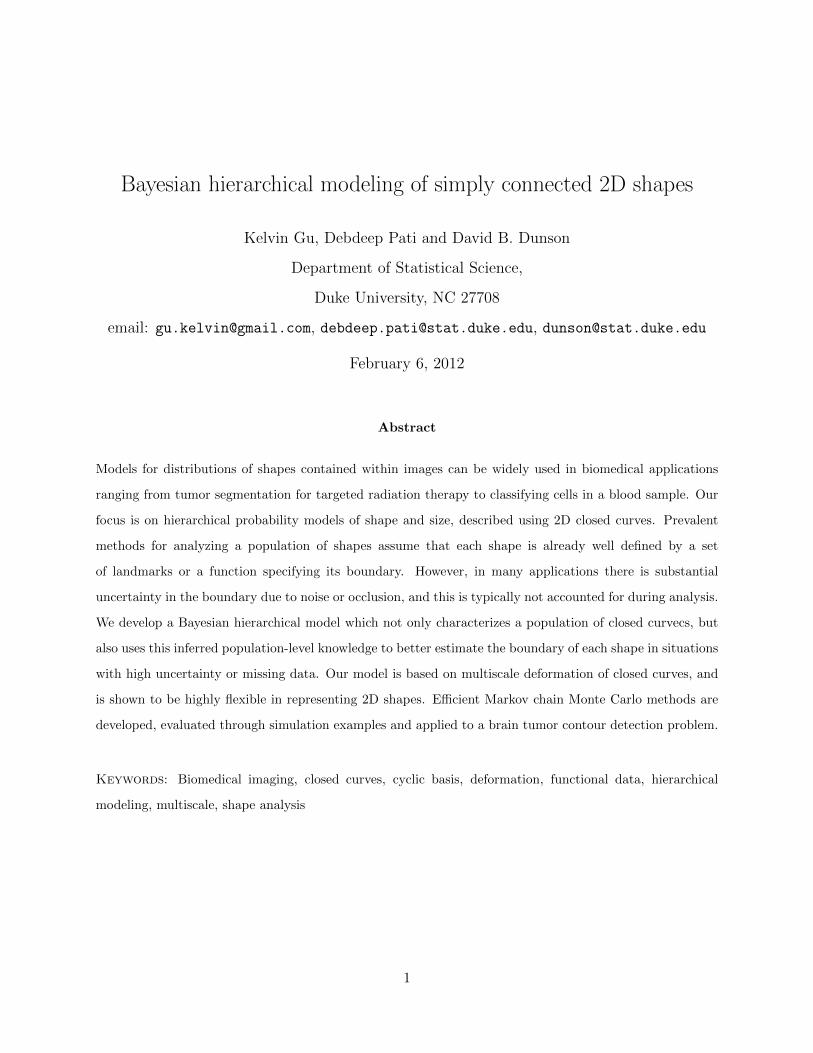
A Roth curve can be deformed simply by translating some of its control points. We now formally define

deformation and illustrate it in Figure 1.

Definition Suppose we are given two Roth curves,

C(t) =JX

j=1

cjBj(t), eC(t) =JX

j=1

ecjBj(t), (3)

5

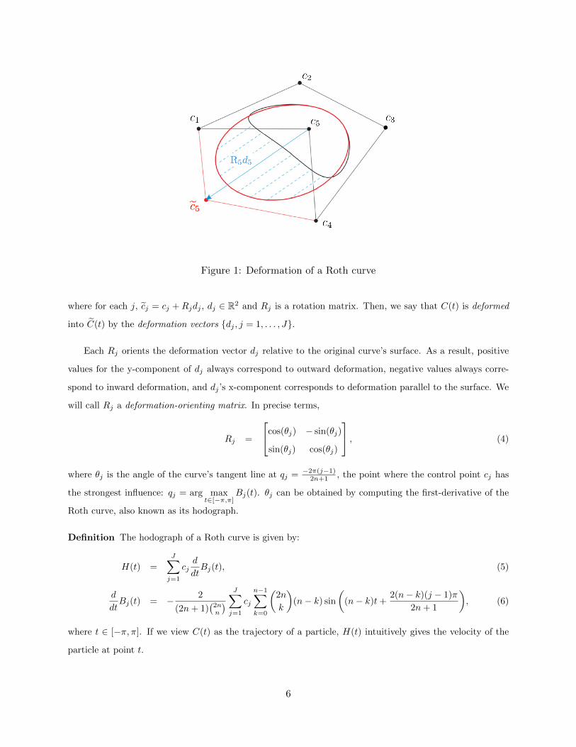
Figure 1: Deformation of a Roth curve

where for each j, ecj = cj + Rjdj , dj 2 R2 and Rj is a rotation matrix. Then, we say that C(t) is deformed

into eC(t) by the deformation vectors {dj , j = 1, . . . , J}.

Each Rj orients the deformation vector dj relative to the original curve’s surface. As a result, positive

values for the y-component of dj always correspond to outward deformation, negative values always corre-

spond to inward deformation, and dj ’s x-component corresponds to deformation parallel to the surface. We

will call Rj a deformation-orienting matrix. In precise terms,

Rj =

2

4

cos(✓j) � sin(✓j)

sin(✓j) cos(✓j)

3

5 , (4)

where ✓j is the angle of the curve’s tangent line at qj = �2⇡(j�1)2n+1 , the point where the control point cj has

the strongest influence: qj = arg maxt2[�⇡,⇡]

Bj(t). ✓j can be obtained by computing the first-derivative of the

Roth curve, also known as its hodograph.

Definition The hodograph of a Roth curve is given by:

H(t) =JX

j=1

cjd

dtBj(t), (5)

d

dtBj(t) = �

2

(2n+ 1)�2nn

�

JX

j=1

cj

n�1X

k=0

✓

2n

k

◆

(n� k) sin

✓

(n� k)t+2(n� k)(j � 1)⇡

2n+ 1

◆

, (6)

where t 2 [�⇡,⇡]. If we view C(t) as the trajectory of a particle, H(t) intuitively gives the velocity of the

particle at point t.

6

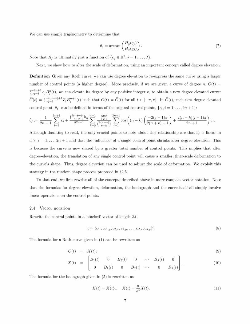
We can use simple trigonometry to determine that

✓j = arctan

✓

Hy(qj)

Hx(qj)

◆

. (7)

Note that Rj is ultimately just a function of {cj 2 R2, j = 1, . . . , J}.

Next, we show how to alter the scale of deformation, using an important concept called degree elevation.

Definition Given any Roth curve, we can use degree elevation to re-express the same curve using a larger

number of control points (a higher degree). More precisely, if we are given a curve of degree n, C(t) =P2n+1

j=1 cjBnj (t), we can elevate its degree by any positive integer v, to obtain a new degree elevated curve:

bC(t) =P2(n+v)+1

j=1 bcjBn+vj (t) such that C(t) = bC(t) for all t 2 [�⇡,⇡]. In bC(t), each new degree-elevated

control point, bcj , can be defined in terms of the original control points, {ci, i = 1, . . . , 2n+ 1}:

bcj :=1

2n+ 1

2n+1X

i=1

ci +

�2(n+v)n+v

�

hn

22n�1

n�1X

k=0

�2nk

�

�2(n+v)v+k

�

2n+1X

i=1

cos

✓

(n� k)

✓

�2(j � 1)⇡

2(n+ v) + 1

◆

+2(n� k)(i� 1)⇡

2n+ 1

◆

ci.

Although daunting to read, the only crucial points to note about this relationship are that bcj is linear in

ci’s, i = 1, . . . , 2n + 1 and that the ‘influence’ of a single control point shrinks after degree elevation. This

is because the curve is now shared by a greater total number of control points. This implies that after

degree-elevation, the translation of any single control point will cause a smaller, finer-scale deformation to

the curve’s shape. Thus, degree elevation can be used to adjust the scale of deformation. We exploit this

strategy in the random shape process proposed in §2.5.

To that end, we first rewrite all of the concepts described above in more compact vector notation. Note

that the formulas for degree elevation, deformation, the hodograph and the curve itself all simply involve

linear operations on the control points.

2.4 Vector notation

Rewrite the control points in a ‘stacked’ vector of length 2J ,

c = (c1,x, c1,y, c2,x, c2,y, . . . , cJ,x, cJ,y)0. (8)

The formula for a Roth curve given in (1) can be rewritten as

C(t) = X(t)c (9)

X(t) =

2

4

B1(t) 0 B2(t) 0 · · · BJ(t) 0

0 B1(t) 0 B2(t) · · · 0 BJ(t)

3

5 . (10)

The formula for the hodograph given in (5) is rewritten as

H(t) = ˙X(t)c, X(t) =d

dtX(t). (11)

7

Deformation can be written as

ec = c+ T (c)d, d = (d1,x, d1,y, d2,x, d2,y, . . . , dJ,x, dJ,y)0, T (c) = block(R1, R2, . . . , RJ), (12)

where block(A1, . . . , Aq) is a pq ⇥ pq block diagonal matrix using p⇥ p matrices Ai, i = 1, . . . , q. We call T

the stacked deformation-orientating matrix. Note that T is a function of c, because each Rj depends on c.

Degree elevation can be written as the linear operator, E:

bc = Ec, E = (Ei,j)n+v,ni=1,j=1.

where

Ei,j =1

2n+ 1+

�2(n+v)n+v

�

hn

22n�1

n�1X

k=0

�2nk

�

�2(n+v)v+k

�

cos

(n� k)

⇢

�2(i� 1)⇡

2(n+ v) + 1

�

+2(n� k)(j � 1)⇡

2n+ 1

�

.

We will maintain this vector notation throughout the rest of the paper.

2.5 Random Shape Process

The random shape process starts with some initial Roth curve, specified by an initial set of control points,

c(0). From here on, we will refer to all curves by the stacked vector of their control points, c. Then, drawing on

the deformation and degree-elevation operations defined earlier, we repeatedly apply the following recursive

operation R times:

bc(r�1) = Erc(r�1), d(r) ⇠ N(µr,⌃r), c(r) = bc(r�1) + Tr(c

(r�1))d(r) (13)

resulting in a final curve c(R). In other words, (i) degree elevate the current curve, (ii) randomly deform it,

and repeat a total of R times. This random process specifies a probability distribution over c(R).

We now elaborate on the details of this recursive process. The parameters of the process are

1. R 2 Z, the number of steps in the process.

2. nr 2 Z, the degree of the curve c(r), for each r = 0, . . . , R. The sequence of {nr}R0 must be strictly

monotonically increasing. For convenience, we will denote the number of control points at a certain

step r to be Jr = 2nr + 1.

3. µr 2 R2Jr , the average set of deformations applied at step r = 0, . . . , R. Note that this vector contains

a stack of deformations, not just one.

4. ⌃r 2 R2Jr

⇥2Jr , the covariance in the set of deformations applied at step r = 0, . . . , R.

For these parameters, Er is the degree-elevation matrix going from degree nr�1to nr, N(·, ·) is a 2Jr-variate

normal distribution and Tr is the stacked deformation orienting matrix.

8

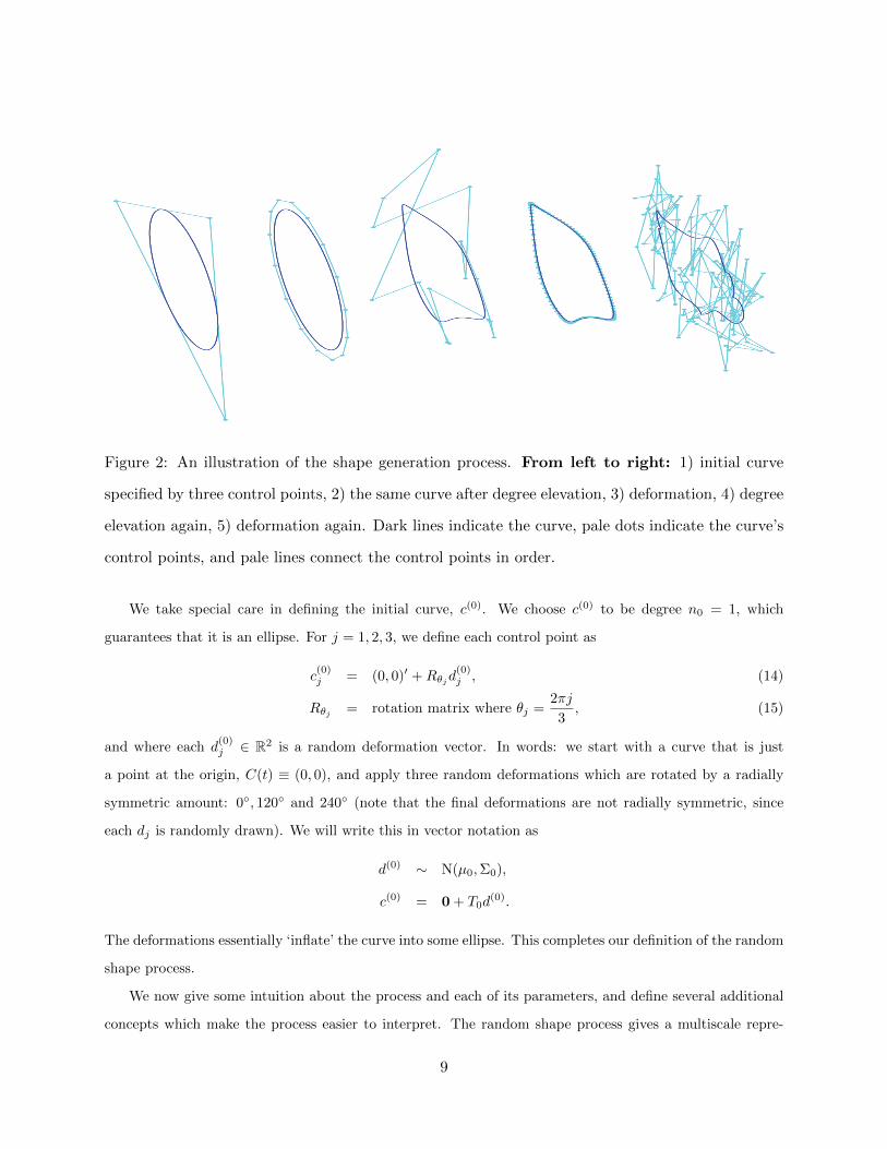
Figure 2: An illustration of the shape generation process. From left to right: 1) initial curve

specified by three control points, 2) the same curve after degree elevation, 3) deformation, 4) degree

elevation again, 5) deformation again. Dark lines indicate the curve, pale dots indicate the curve’s

control points, and pale lines connect the control points in order.

We take special care in defining the initial curve, c(0). We choose c(0) to be degree n0 = 1, which

guarantees that it is an ellipse. For j = 1, 2, 3, we define each control point as

c(0)j = (0, 0)0 +R✓j

d(0)j , (14)

R✓j

= rotation matrix where ✓j =2⇡j

3, (15)

and where each d(0)j 2 R2 is a random deformation vector. In words: we start with a curve that is just

a point at the origin, C(t) ⌘ (0, 0), and apply three random deformations which are rotated by a radially

symmetric amount: 0�, 120� and 240� (note that the final deformations are not radially symmetric, since

each dj is randomly drawn). We will write this in vector notation as

d(0) ⇠ N(µ0,⌃0),

c(0) = 0+ T0d(0).

The deformations essentially ‘inflate’ the curve into some ellipse. This completes our definition of the random

shape process.

We now give some intuition about the process and each of its parameters, and define several additional

concepts which make the process easier to interpret. The random shape process gives a multiscale repre-

9

sentation of shapes, because each step in the process produces increasingly fine-scale deformations, through

degree-elevation.

R is then the number of scales or ‘resolutions’ captured by the process. Each nr specifies the number of

control points at resolution r. We will use Sr to denote the class of shapes that can be exactly represented

by a degree nr Roth curve. If {nr}R1 is monotonically increasing, then S1 ⇢ S2 ⇢ . . . ⇢ SR. Thus, the

deformations d(r) roughly describe the additional details gained going from Sr�1 to Sr.

µr is the mean deformation at level r. Based on {µr, r = 0, . . . , R}, we define the ‘central shape’ of the

random shape process, cµ as:

cµ := c(R)µ

c(r)µ = Erc(r�1)µ + Tr(c

(r�1)µ )µr

Note that c⇤ is simply the deterministic result of the random shape process when each d(r) = µr, rather

than being drawn from a distribution centered on µr. Thus, all shapes generated by the process tend to be

deformed versions of the central shape. We illustrate this in Figure 3. If the random shape process is used

to describe a population of shapes, the central shape provides a good summary.

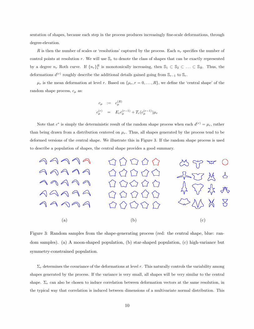
(a) (b) (c)

Figure 3: Random samples from the shape-generating process (red: the central shape, blue: ran-

dom samples). (a) A moon-shaped population, (b) star-shaped population, (c) high-variance but

symmetry-constrained population.

⌃r determines the covariance of the deformations at level r. This naturally controls the variability among

shapes generated by the process. If the variance is very small, all shapes will be very similar to the central

shape. ⌃r can also be chosen to induce correlation between deformation vectors at the same resolution, in

the typical way that correlation is induced between dimensions of a multivariate normal distribution. This

10

allows us to incorporate higher-level assumptions about shape, such as reflected or radial symmetry. For

example, if R = 2, n1 = 1 and n2 = 2, we can specify perfect correlation in ⌃2, such that d(2)1 = d(2)4 and

d(2)2 = d(2)3 . The resulting shapes are guaranteed to be symmetrical along an axis of reflection.

In the subsequent sections 4 and 5, we show how to use our random shape process to guide curve-fitting

for various types of data.

3. PROPERTIES OF THE PRIOR

3.1 General notations

The supremum and L1-norm are denoted by || · ||1 and || · ||1, respectively. We let || · ||p,⌫ denote the

norm of Lp(⌫), the space of measurable functions with ⌫-integrable pth absolute power. The notation C(X )

is used for the space of continuous functions f : X ! R endowed with the uniform norm. For ↵ > 0

, we let C↵(X ) denote the Holder space of order ↵, consisting of the functions f 2 C(X ) that have b↵c

continuous derivatives with the b↵cth derivative fb↵c being Lipschitz continuous of order ↵�b↵c. We write

“-” for inequality up to a constant multiple and {a(1), a(2), . . . , a(n)} to denote the order statistics of the set

{ai : ai 2 R, i = 1, . . . , n}.

3.2 Support

Let the Holder class of periodic functions on [�⇡,⇡] of order ↵ be denoted by C↵([�⇡,⇡]). Define the class

of closed parametric curves SC(↵1,↵2) having di↵erent smoothness along di↵erent coordinates as

SC(↵1,↵2) := {S = (S1, S2) : [�⇡,⇡] ! R2, Si2 C↵

i([�⇡,⇡]), i = 1, 2}. (16)

Consider for simplicity a single resolution Roth curve with control points {cj , j = 0, . . . , 2n}. Assume

we have independent Gaussian priors on each of the two coordinates of cj for j = 0, . . . , 2n, i.e., C(t) =P2n

j=0 cjBnj (t), cj ⇠ N2(0,�2

j I2), j = 0, . . . , 2n. Denote the prior for C by ⇧Cn . ⇧Cn defines an independent

Gaussian process for each of the components of C. Technically speaking, the support of a prior is defined

as the smallest closed set with probability one. Intuitively, the support characterizes the variety of prior

realizations along with those which are in their limit. We construct a prior distribution to have large

support so that the prior realizations are flexible enough to approximate the true underlying target object.

As reviewed in van der Vaart and van Zanten (2008), the support of a Gaussian process (in our case ⇧Cn)

is the closure of the corresponding reproducing kernel Hilbert space (RKHS). The following Lemma 3.1

describes the RKHS of ⇧Cn , which is a special case of Lemma 2 in Pati and Dunson (2011).

11

Lemma 3.1 The RKHS Hn of ⇧Cn consists of all functions h : [�⇡,⇡] ! R2 of the form

h(t) =2nX

j=0

cjBnj (t) (17)

where the weights cj range over R2. The RKHS norm is given by

||h||2Hn

=2nX

j=0

||cj ||2/�2

j . (18)

The following theorem describes how well an arbitrary closed parametric surface S0 2 SC(↵1,↵2) can be

approximated by the elements of Hn for each n. Refer to Appendix A for a proof.

Theorem 3.2 For any fixed S0 2 SC(↵1,↵2), there exists h 2 Hn with ||h||2Hn

K1P2n

j=0 1/�2j such that

||S0 � h||1 K2n�↵(1) log n (19)

for some constants K1,K2 > 0 independent of n.

This shows that the Roth basis expansion is su�ciently flexible to approximate any closed curve arbitrarily

well. Although we have only shown large support of the prior under independent Gaussian priors on the

control points, the multiscale structure should be even more flexible and hence rich enough to characterize

any closed curve. We can also expect minimax optimal posterior contraction rates using the prior ⇧Cn

similar to Theorem 2 in Pati and Dunson (2011) for suitable choices of prior distributions on n.

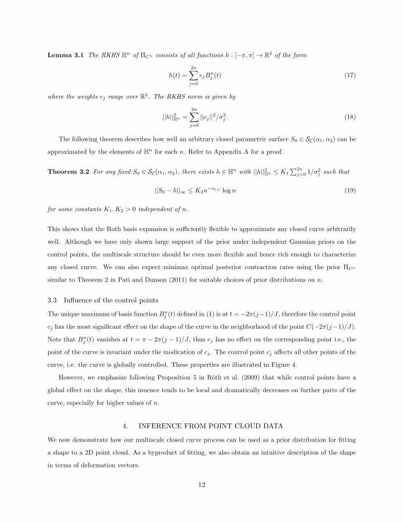
3.3 Influence of the control points

The unique maximum of basis function Bnj (t) defined in (1) is at t = �2⇡(j�1)/J , therefore the control point

cj has the most significant e↵ect on the shape of the curve in the neighborhood of the point C(�2⇡(j�1)/J).

Note that Bnj (t) vanishes at t = ⇡ � 2⇡(j � 1)/J , thus cj has no e↵ect on the corresponding point i.e., the

point of the curve is invariant under the modication of cj . The control point cj a↵ects all other points of the

curve, i.e. the curve is globally controlled. These properties are illustrated in Figure 4.

However, we emphasize following Proposition 5 in Roth et al. (2009) that while control points have a

global e↵ect on the shape, this inuence tends to be local and dramatically decreases on further parts of the

curve, especially for higher values of n.

4. INFERENCE FROM POINT CLOUD DATA

We now demonstrate how our multiscale closed curve process can be used as a prior distribution for fitting

a shape to a 2D point cloud. As a byproduct of fitting, we also obtain an intuitive description of the shape

in terms of deformation vectors.

12

Figure 4: Influence of the control point on the Roth curve

Assume that the data consist of points {pi 2 <

2, i = 1, . . . , N} concentrated near a 2D closed curve.

Since a Roth curve can be thought of as a function expressing the trajectory of a particle over time, we view

each data point, pi, as a noisy observation of the particle’s location at a given time ti,

pi = C(ti) + ✏i, ✏i ⇠ N2(0,�2I2). (20)

(20) shares a similar form to nonlinear factor models, where ti is the latent factor score. First, we will rewrite

the point cloud model in stacked vector notation. Defining

p = (p1,x, p1,y, . . . , pN,x, pN,y)0, ✏ = (✏1,x, ✏1,y, . . . , ✏N,x, ✏N,y)

0

t = (t1,x, t1,y, . . . , tN,x, tN,y)0, X(t)0 = [X(t1)

0X(t2)0 . . . X(tN )0]

we have

p = X(t)c+ ✏, ✏ ⇠ N2N (0,�2I2N ) (21)

where X(ti) is as defined in (11).

To fit a Roth curve through the data, we want to infer P (c | p), the posterior distribution over control

points c, given the data points p. To compute this, we must specify P (p | c), the likelihood, and P (c),

the prior distribution over Roth curves. We choose P (c) to be the probability distribution induced by the

shape-generating random process specified in §2.5. From (21), we can specify the likelihood function as,

P ({pi}N1 | {ci}

J1 ) =

NY

i=1

N2

✓

pi;JX

j=1

cjBj(ti),�2I2

◆

, (22)

P (p | c) = N2N (p;X(t)c,�2I2N ). (23)

This completes the Bayesian formulation for inferring c, given p and t. In §7, we describe the exact method

for performing Bayesian inference.

13

In many applications, ti is not known and can be treated as a latent variable. We propose a prior for ti

conditionally on c, which is designed to be uniform over the curve’s arc-length. This prior is motivated by

the frequentist literature on arc-length parameterizations (Madi 2004), but instead of assigning the values

{ti 2 [�⇡,⇡]} in a deterministic preliminary step prior to statistical analysis, we use a Bayesian approach

to formally accommodate uncertainty in parameterization of the points. Define the arc-length function

A : [�⇡,⇡] 7! R+

A(u) := A(u; (c0, . . . , c2n)) =

Z u

�⇡

||H(t)||dt. (24)

Note that A is monotonically increasing and satisfies A(�⇡) = 0, A(⇡) = L(c0, . . . , c2n) where L(c0, . . . , c2n)

is the length of the curve conditional on the control points (c0, . . . , c2n) and is given byR ⇡

�⇡||H(t)||dt.

Given (c0, . . . , c2n), we draw li ⇠ Unif(0, L(c0, . . . , c2n)) and set ti = A�1(li). Thus we obtain a prior

for the ti’s which is uniform along the length of the curve and is given by

p(t) =||H(t)||

R ⇡

�⇡||H(t)||dt

.

Thus the high velocity regions on the curve are penalized more and the low velocity regions are penalized less

to enable uniform arc-length parameterizations. We will discuss a griddy Gibbs algorithm for implementing

the arc-length parametrization in a fully Bayesian framework in §7.

5. INFERENCES FROM PIXELATED IMAGE DATA

In this section, we show how to model image data by converting it to point cloud data. We also show how

image data gives a bonus estimate for the object’s surface orientation, !i at each point pi. We incorporate this

extra information into our model to improve fitting, with essentially no sacrifice in computational e�ciency.

A grayscale image can be treated as a function Z : R2! R. The gradient of this function, rZ : R2

! R2

is a vector field, where rZ(x, y) is a vector pointing in the direction of steepest ascent at (x, y). In computer

vision, it is well known that the gradient norm of the image, ||rZ||2 : R2! R approximates a ‘line-drawing’

of all the high-contrast edges in the image. Our goal is to fit the edges in the image with our shape model.

In practice, an image is discretized into pixels {za,b | a = 1, . . . , X, b = 1, . . . , Y } but a discrete version

of the gradient can still be computed by taking the di↵erence between neighboring pixels, such that one

gradient vector, ga,b is computed at each pixel. The image’s gradient norm is then just another image, where

each pixel ma,b = ||ga,b||2.

Finally, we extract a point cloud: {(a, b) | ma,b > M, a = 1, . . . , X, b = 1, . . . , Y } where M is some

user-specified threshold. Each point (a, b) can still be matched to a gradient vector ga,b. For convenience, we

will re-index them as pi and gi. The gradient vector points in the direction of steepest change in contrast, i.e.

14

it points across the edge of the object, approximating the object’s surface normal. The surface orientation

is then just !i = arctan( gi,ygi,x

).

In the following, we describe a model relating a Roth curve to each !i. This model can be used together

with the model we specified earlier for the pi.

5.1 Modeling surface orientation

Denote by vi = (Hx(ti), Hy(ti)) 2 R2 the velocity vector of the curve C(t) at the parameterization location

ti, i = 1, . . . , N . Note that vi is always tangent to the curve. Since each !i points roughly normal to the

curve, we can rotate all of them by 90 degrees, ✓i = !i +⇡2 , and treat each ✓i as a noisy estimate of vi’s

orientation. Note that we cannot rotate the vector gi by 90 degrees and directly treat it as a noisy observation

of vi. In particular, gi ’s magnitude bears no relationship to the magnitude of vi: ||gi|| is the rate of change

in image brightness when crossing the edge of the shape, while ||vi|| describes the speed at which the curve

passes through pi.

Suppose we did have some noisy observation of vi, denoted ui. Then, we could have specified the following

linear model relating the curve {cj , j = 1, . . . , J} to the ui’s:

ui = vi + �i (25)

=JX

j=1

cjd

dtBj(ti) + �i (26)

for i = 1, . . . , N where �i ⇠ N2(0, ⌧2I2). Instead, we only know the angle of ui, ✓i. In §7, we show that using

this model, we can still write the likelihood for ✓i, by marginalizing out the unknown magnitude of ui. The

resulting likelihood still results in conditional conjugacy of the control points.

6. FITTING A POPULATION OF SHAPES

We can extend our methodology in the previous section to simultaneously fit and characterize a collection of

K separate point clouds, via hierarchical modeling. In the previous section, we used the random shape process

as a prior with fixed parameters. Now, we will instead treat the random shape process as a latent mechanism

which generated all K shapes. The inferred parameters of the latent shape process then characterize the

collection of shapes.

As a reminder, the parameters of the random shape process and their interpretations are defined in §2.5.

Rather than fixing their values, we will treat µr and ⌃r for r = 0, . . . , R as unknowns and place the following

priors on them:

15

µr ⇠ N2Jr

(µµr

,⌃µr

),

⌃�1r = diag

✓

h

⌧ (r)1,x , ⌧(r)1,y , ⌧

(r)2,x , ⌧

(r)2,y , · · · , ⌧

(r)Jr

,x, ⌧(r)Jr

,y

i0◆

,

⌧ (r)u ⇠ Gamma (↵⌧ ,�⌧ ) for u = {1, . . . Jr}⇥ {x, y},

where diag (v) takes any vector v 2 Rd and produces the diagonal matrix V 2 Rd⇥d with elements of v along

the diagonal. We will continue to treat R and {nr | r = 0, . . . , R} as fixed, although we plan to consider in-

ferring these quantities in future work. Note that the prior on ⌃r only permits diagonal covariance structure,

assuming independence between deformations (and between the x/y components of each deformation). In

future work, it will be interesting to remove this simplifying assumption and characterize inter-deformation

correlation. Nonetheless, the inferred values ofn

⌧ (r)u | u = {1, . . . Jr}⇥ {x, y}, r = 0, . . . , Ro

can still be use-

fully interpreted. For example, a high value for ⌧ (R)2,y indicates that there is a high-level of variability in

the second deformation vector at resolution R (implying a fairly fine-scale deformation). Since it is the

y-component, this corresponds to variability normal to the shape surface.

We now formalize the concept that all K shapes are generated from a single random shape process.

Denote the kth point cloud as pk for k = 1, . . .K. Each pk is fit by a curve ck, which is composed from the

deformations�

d(r),k | r = 0, . . . , R

and each d(r),k ⇠ N (µr,⌃r). This hierarchical structure also induces

dependence between the K shapes, enabling curves to borrow information from each other during fitting.

An additional challenge that arises from modeling multiple shapes is inter-shape alignment (also known

as registration). This typically involves removing di↵erences in object position, orientation and scale. Here,

we only deal with position and orientation. According to (14), our random shape process generates shapes

centered at (0, 0) and rotated to a fixed angle. However, in an actual population of shapes, each shape is

rotated to a di↵erent angle and centered at a di↵erent location. We can modify (14) to account for this

simply by adding parameters for the position, mk2 R2, and orientation, �k

2 [�⇡,⇡], of each object k:

c(0)j = mk +R�kR✓j

d(0)j ,

where R�k is a rotation matrix. In the experiments we perform, we manually set �k for each object k. The

orientation of level r = 0 orients all subsequent levels. This is su�cient to align the entire population and

make the deformation vectors of each shape directly comparable.

We also note that the definition of �k has an important anchoring e↵ect on tk. The prior for tk is

conditional on the curve ck. Since the random shape process prior for the curve is oriented by �k, the prior

for tk favors parametrizations that conform to this orientation.

16

7. POSTERIOR COMPUTATION

In §6, we presented a model for characterizing and fitting a population of K closed curves, with unknown

underlying parametrization. We now present an MCMC algorithm for sampling from the joint posterior of

this model. This involves deriving the conditional posteriors of mk, d(r),k, µr,⌃r and tk for r = 0, . . . , R and

k = 1, . . . ,K.

7.1 Conditional posteriors for mk and d(r),k

The conditional posteriors for mk and d(r),k are the most challenging to sample from, because our model’s

likelihood function is nonlinear in these terms, preventing conditional conjugacy. To overcome this, we derive

a linear approximation to the true likelihood function, which does yield conditional conjugacy, and then use

samples from the approximate conditional posterior as proposals in a Metropolis-Hastings step.

We first present the source of nonlinearity in the likelihood function. Recall from §4 that:

P (pk | c(R),k) = N2N (pk;X(tk)c(R),k,�2I2N ).

From §2.5, we note that c(R),k is the result of combining the deformations�

d(r),k | r = 0, . . . , R

through

the following recursive relation, with mk appearing in the base case:

c(r),k = Erc(r�1),k + Tr

⇣

c(r�1),k⌘

d(r),k (27)

c(0),k = mk + T�kT0d(0),k (28)

At each step r of the recursive process, the deformation-orienting matrix Tr is a nonlinear function of the

previous c(r�1),k. As a result, c(R),k is nonlinear in d(r),k for r = 0, . . . , R � 1. For any given step of

the process, we can replace the true recursive relation with a linear approximation. In particular, we will

substitute Tr(c(r�1),k)d(r),k with Tr,kc(r�1),k, where Tr,k will be derived shortly. The new approximate step

is then

c(r),k ⇡

⇣

Er + Tr,k

⌘

c(r�1),k. (29)

If we wish to write c(R),k linearly in terms of c(r),k for any r = 0, . . . , R, we can replace every recursive

step from r to R with the approximate step given in (29). We emphasize that steps 0, . . . r � 1 follow the

original recursive relation. This yields the following approximation:

c(R),k⇡ ⌦R

r+1c(r),k, ⌦b

a =

8

>

>

>

<

>

>

>

:

bY

⇢=a

⇣

E⇢ + T⇢,k

⌘

if a < b

1 otherwise.

(30)

17

Now, by combining (27) and (30), we have that:

c(R),k⇡

8

>

<

>

:

⌦Rr+1

⇥

Erc(r�1),k + Tr

�

c(r�1),k�

d(r),k⇤

r > 0

⌦R1

�

mk + T�kT0d(0),k�

r = 0

Thus, the approximation of c(R),k can be written linearly in terms of any d(r),k or mk. Note that it is

still nonlinear in d(⇢),k for any ⇢ 6= r. However, for MCMC sampling, we only need one d(r),k to be linear

at a time, holding all others fixed. Lastly, we note that the approximation becomes increasingly good as r

approaches R, because the number of approximate steps (contained in ⌦ba) decrease.

We are now ready to derive the approximate conditional posteriors for mk and d(r),k. First, we claim

that these posteriors can all be written in the following form for generic ‘x’, ‘y’ and ‘z’.

P (x | �) / N(y;Qx,⌃y) N (x; z,⌃x) (31)

P (x | �) = N⇣

µ, ⌃⌘

, ˆ⌃�1 = ⌃�1x +

X

k

Q0⌃�1y Q, µ = ⌃

⌃�1x z +

X

k

Q0⌃�1y y

!

. (32)

Note that each approximate conditional posterior is simply a multivariate normal. We now show that each

approximate posterior can be rearranged to match the form of (31) - (32).

Papprox(mk| �) / N

⇣

pk;X(tk)c(R),k,�2I2Nk

⌘

N(mk;µm,⌃m)

/ N⇣

pk;X(tk)⌦R,k1

⇣

mk + T0d(0),k

⌘

,�2I2Nk

⌘

N(mk;µm,⌃m)

/ N⇣

pk � X(tk)⌦R,k1 T0d

(0),k;X(tk)⌦R,k1 mk,�2I2Nk

⌘

N(mk;µm,⌃m)

Papprox(d(r),k

| �) / N⇣

pk;X(tk)c(R),k,�2I2Nk

⌘

N(d(r),k;µr,⌃r)

/ N⇣

pk;X(tk)⌦Rr+1

h

Erc(r�1),k + Tr

⇣

c(r�1),k⌘

d(r),ki

,�2I2Nk

⌘

N(d(r),k;µr,⌃r)

/ N⇣

pk � X(tk)⌦Rr+1Erc

(r�1),k;X(tk)⌦Rr+1Tr

⇣

c(r�1),k⌘

d(r),k,�2I2Nk

⌘

N(d(r),k;µr,⌃r)

We then use Papprox(mk| �) and Papprox(d(r),k | �) as M-H proposal distributions to sample from their

true counterparts. Both are multivariate normals and if necessary, their variance parameters may be tuned

to improve sampling e�ciency.

7.2 Derivation of the approximate deformation-orienting matrix, T

For visual clarity of the derivation, we will temporarily drop superscripts denoting the resolution r and object

index k of each variable. First, we recall from §2 that T (c) is a block diagonal matrix with blocks consisting

of the rotation matrices Rj , for j = 1, . . . , J (where J is the total number of control points at the particular

resolution r). Each Rj rotates its corresponding deformation, dj , by ✓j = arctan⇣

Hy

(qj

)H

x

(qj

)

⌘

. Now, using the

18

identities

cos(arctan(x/y)) =x

p

x2 + y2, sin(arctan(x/y)) =

yp

x2 + y2,

we can write Rj as:

Rj =1

sj(c)

2

4

Hx(qj) �Hy(qj)

Hy(qj) Hx(qj)

3

5

where sj(c) =p

Hx(qj)2 +Hy(qj)2. This term intuitively represents the “speed” of the curve at parametric

position qj . It is reasonable to think that the curve’s speed does not vary greatly among samples in the

posterior, because in §4 we imposed a prior that encourages arc-length uniform parametrization, and because

the total arc-length of the curve is not expected to vary greatly. Therefore, we approximate this term with

the fixed constant Sj = sj(cprev), where cprev is just the curve sampled in the previous iteration of the

M-H sampler. Lastly note that the hodograph, H (t) = X(t)c, is a linear function of c. So, we can now

approximate Rj as a linear function of c:

Rj ⇡

1

Sj

2

4

Xx(qj,)c �Xy(qj)c

Xy(qj)c Xx(qj)c

3

5 .

Then, we can write Rjdj as:

Rjdj ⇡ Rjc, Rj =1

Sj

2

6

4

⇣

Xx(qj,)dj,x � Xy(qj)dj,y⌘

⇣

Xy(qj)dj,x � Xx(qj)dj,y⌘

3

7

5

,

and finally we define T = block⇣

R1, . . . , RJ

⌘

.

7.3 Conditional posteriors for µr and ⌃r

P (µr | �) = N⇣

µr, ⌃µr

⌘

⌃�1µr

= ⌃�1µr

+K⌃�1r

µr = ⌃µr

⌃�1µr

µµr

+ ⌃�1r

KX

k=1

d(r),k!

P

✓

⌃r = diag⇣

⌧ (r)1,x , ⌧(r)1,y , ⌧

(r)2,x , ⌧

(r)2,y , · · · , ⌧

(r)Jr

,x, ⌧(r)Jr

,y

⌘�1| �

◆

=Jr

Y

j=1

P⇣

⌧ (r)j,x | �

⌘

P⇣

⌧ (r)j,y | �

⌘

P (⌧ (r)j,x | �) = Ga⇣

↵(r)j,x, �

(r)j,x

⌘

↵(r)j,x = ↵⌧ +K �(r)

j,x = �⌧ +

KX

k=1

⇣

d(r),kj,x � µr,j,x

⌘2

2

19

7.4 Griddy Gibbs updates for the parameterizations tki

We discretize the possible values of tki 2 [�⇡,⇡] to obtain a discrete approximation of its conditional posterior:

tki | � ⇠

N(pki ;X(ti)c(R),k,�2I2)P (tki | c(R),k)P

⌧2[�⇡,⇡] N(pki ;X(⌧)c(R),k,�2I2)P (tki | c(R),k)

We can make this arbitrarily accurate, by making a finer summation over ⌧ .

7.5 Likelihood contribution from surface-normals

Define

Xx(ti) =

dBn10 (ti)

dt, 0,

dBn11 (ti)

dt, 0, · · · ,

dBn12n1

(ti)

dt, 0

�

(33)

Xy(ti) =

0,dBn1

0 (ti)

dt, 0,

dBn11 (ti)

dt, · · · , 0,

dBn12n1

(ti)

dt

�

(34)

Proposition 1 The likelihood contribution of the tangent directions ✓ki , i = 1, . . . , Nk ensures conjugate

updates of the control points for a multivariate normal prior.

Proof Recall the noisy tangent direction vectors uki ’s and vki ’s in (25). Using a simple reparameterization

uki = (eki , e

ki tan ✓

ki )

where only ✓0is are observed and ei’s aren’t. Observe that

vki = (Hx(ti), Hy(ti)) = (Xx(tki )c

(3),k, Xy(tki )c

(3),k). (35)

Assuming a uniform prior for the mki ’s on R, the marginal likelihood of the tangent direction ✓ki given ⌧2

and the parameterization tki is given by

l(✓ki ) =1

2⇡⌧2

Z 1

�1exp

�

1

2⌧2{(eki � Xx(t

ki )c

(3),k)2 + (eki tan(✓i)� Xy(tki )c

(3),k)2}

�

deki

It turns out the above expression has a closed form given by

l(✓ki ) =1

2⇡⌧2

p

2⇡⌧2p

1 + tan2(✓ki )exp

"

�

1

2⌧2

(

(Xx(tki )c

(3),k)2 + (Xy(tki )c

(3),k)2 �(Xx(tki )c

(3),k + Xy(tki )c(3),k tan(✓i))2

1 + tan2(✓ki )

)#

.

The likelihood for the {✓ki , i = 1, . . . , Nk} is given by

L(✓k1 , . . . , ✓kNk

) /

1

⌧Nk

exp

2

4

�

1

2⌧2

Nk

X

i=1

(Xx(tki )c(3),k)2 tan2(✓i) + (Xy(tki )c

(3),k)2 � 2Xx(tki )c(1),kXy(tki )c

(1),k tan(✓i)

1 + tan2(✓i)

3

5

=1

⌧Nk

exp

"

�

1

2⌧2(c(3),k)0

(

NX

i=1

(T ki )

0⌃ki T

ki

)

c(3),k#

20

where

⌃i =

0

@

tan2(✓k

i

)1+tan2(✓k

i

)� tan(✓k

i

)1+tan2(✓k

i

)

� tan(✓k

i

)1+tan2(✓k

i

)1

1+tan2(✓k

i

)

1

A

and Ti = [(Xx(tki ))0 (Xy(tki )

0] is a 2(2n3+1)⇥2 matrix. Clearly, an inverse-Gamma for ⌧2 and a multivariate

normal prior for the control points are conjugate choices. ⇤

7.6 Approximate Bayesian Multiresolution Sampler

One encounters some practical issues when running the MCMC algorithm proposed above. Firstly, there

can be slow mixing caused by high posterior dependence between the unknowns characterizing the curves

at di↵erent levels of resolution. In addition, as the curves at the coarser scales only have an indirect

impact on the likelihood of the data, one encounters identifiability issues, which create problems if one

wishes to interpret the curves at di↵erent resolutions. Identifiability restrictions can be enforced to maintain

interpretability (e.g., curves at di↵erent resolutions have a common area), but such constraints lead to highly

challenging computation.

In the frequentist multiresolution modeling literature, it is standard practice to apply multistage esti-

mation procedures, which fit a curve at one level of resolution, and then proceed to analyze the residuals at

the next level of resolution. Such approaches can have excellent performance in producing a point estimate,

but it is challenging to fully accommodate uncertainty in curve estimation across resolutions.

We accomplish this using a simple approximate Bayesian multiresolution sampler (AB-MS), which is a

typical MCMC algorithm with one important exception - in updating the unknowns specific to a curve at a

given level of resolution, one sets all higher resolution deformations equal to zero. By discarding finer scale

structure in updating course-scale unknowns, we solve the identifiability and mixing issues but no longer

obtain an exact Bayesian procedure. There is a rich precedent in the literature for related approximations;

for example, algorithms for cutting ‘feedback’ in joint modeling (Lunn et al., 2009; McCandless et al., 2010).

8. SIMULATION STUDY

We evaluate our method by defining a true underlying curve, c⇤, and checking to see how accurately this

curve can be recovered by our model under various conditions. We first define several concepts to help

interpret our results. Given some curve c, let B(c) = {X(t)c | t 2 [�⇡,⇡]}(the set of all points along the

curve), and let A(c) denote the interior region enclosed by the curve.

For a given distribution over curves, P (c), we define its boundary heatmap, MBP (c) : R2

! R, and its

21

Figure 5: We generated and fit a point cloud of size (a) N = 10, (b) N = 30 and (c) N = 100.

The points are shown as blue dots. The true curve, c⇤is shown in red. The colored regions are

percentiles of MBP (c|p) (orange: top 30%, cyan: top 50%, blue: top 80%). Note that the bands of

uncertainty shrink as N increases. Also note that there is a wider band of uncertainty where the

data is missing.

region heatmap, MAP (c) : R

2! R, as:

MAP (c) (x, y) = P ((x, y) 2 A (c)) ,

MB (x, y) dxdy = P ((x+ dx, y + dy) \B(c)) .

Given a set of samples from the distribution P (c), {cs | s = 1, . . . , S}, we can discretely approximate MBP (c)

and MAP (c) as:

MBP (c) (x) ⇡ TODO, MA

P (c) (x) ⇡1

S

SX

s=1

1 (x 2 A (cs)) ,

and the mean can be approximated by c = 1S

SX

s=1

cs.

8.1 Inferring shape from a single point cloud

We generate a single point cloud p concentrated along c⇤using the point cloud model defined in §4. To make

the task even more challenging, we also randomly remove a segment of the cloud, resulting in a large gap.

We then infer a curve from the point cloud, using the AB-MS algorithm described in §7.6. We then interpret

its posterior, P (c | p), using its boundary heatmap MBP (c|p) and measure the mean-squared-error between c

and c⇤. For all cases, the hyperparameters of the prior were set to: TODO. The MSE was (a) TODO, (b)

TODO and (c) TODO.

8.2 Inferring shape from multiple point clouds

In the above example on fitting a single point cloud, note that uncertainty is naturally high where the point

cloud contains a gap. This uncertainty can be reduced if the investigator can “borrow information” from

other point clouds known to be from the same population of shapes. In particular, we will assume that

multiple shapes are drawn from the same random shape process, as described in §6, and fit all of them

simultaneously. The hyperparameters of the prior were set to: TODO.

Besides simply fitting each shape in the population, we can also extract information from the inferred

latent variables of our random shape process. In particular, the central shape cµ (defined in §2.5) is iden-

22

Figure 6: From the same true curve c⇤, we generated multiple rotated point clouds. Note that the

gaps in each shape are intelligently fit with shape information borrowed from other members of the

population. All colors and indicators are the same as in Figure ??.

tifiable and provides a useful summary of the entire population. In the following example, we generate 16

randomly deformed instances of c⇤and fit the resulting point clouds (for visual clarity, we have limited the

noise of these point clouds). The posterior distribution for cµsuccessfully captures the artificially injected

variability in shape. Again, we interpret P�

cµ |

�

pk �

using its boundary heatmap MBP (c

µ

|{pk}) (just MB

for notational convenience).

8.3 Assessment of mixing, convergence

# of samples, burn in

sensitivity analysis

raftery lewis check for convergence

9. BRAIN TUMOR IMAGING STUDY

In brain tumor diagnosis and therapy, it is very important to account for uncertainty in the tumor’s outline.

This information is crucial for assessing whether a tumor has grown/regressed over time, and even more

important if a surgeon must target the tumor for excision or radiation therapy. In that situation, there is a

critical tradeo↵ between false positives (targeting healthy tissue) and extremely undesirable false negatives

(missing the tumor). Furthermore, tumor outlines are notoriously hard to determine. Error stems from

the poor contrast between tumor and healthy tissue in magnetic resonance imaging (MRI), the prevalent

modality for diagnosis. Even seasoned experts di↵er greatly when tracing an estimate.

We use our model to intelligently combine the input traces of multiple experts, by treating each trace as a

point cloud drawn from the same random shape process. We can then interpret P (cµ | {pk}) as the posterior

distribution of the tumor, fully describing the variability and uncertainty among the experts. One might

also run additional tumor segmentation algorithms, and combine their outputs using the same approach. In

this setting, the region heatmap of the posterior, MAP (c

µ

|{pk

}) (shortened to MA), is especially informative.

For every point x, MA(x) gives the probability that it is part of the tumor. This enables a neurosurgeon to

manage the tradeo↵ between false positives/negatives in a principled manner. Let the true tumor region be

Xtumor ⇢ R2 and X{tumor its complement. Then, define the loss function for targeting a region X to be

L(X) = �+Area⇣

X \X{tumor

⌘

+��Area⇣

X{\Xtumor

⌘

.

23

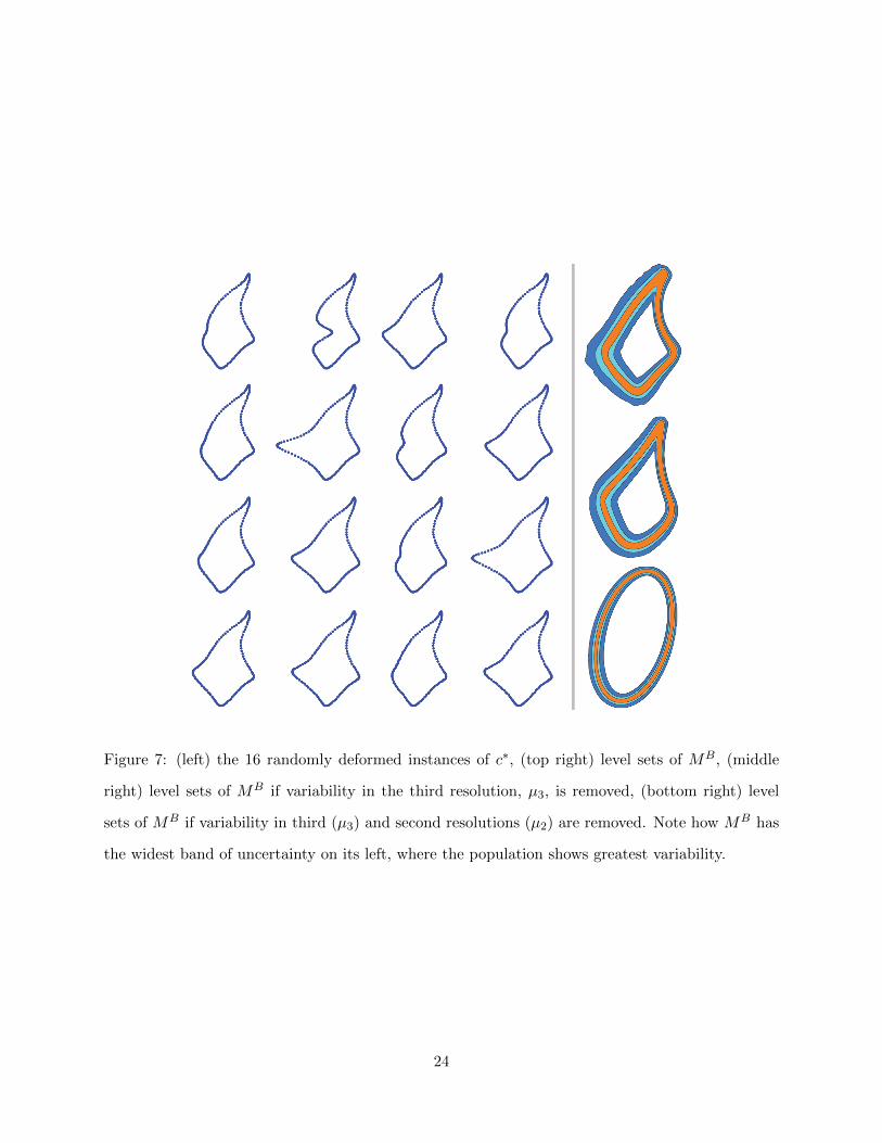
Figure 7: (left) the 16 randomly deformed instances of c⇤, (top right) level sets of MB, (middle

right) level sets of MB if variability in the third resolution, µ3, is removed, (bottom right) level

sets of MB if variability in third (µ3) and second resolutions (µ2) are removed. Note how MB has

the widest band of uncertainty on its left, where the population shows greatest variability.

24

Depending on the ratio of the penalties �+ and ��, the surgeon can minimize L simply by cutting along a

level set of MA.

We can also allow for experts to express varying confidence in di↵erent portions of their trace. This is

desirable, because certain boundaries of the tumor will have high contrast with the surrounding tissue while

other parts won’t, and the expert should not be forced to make an equal opinion on both. We can achieve

this by slightly modifying the point cloud model given in (20). There, we assumed that each point pi was

generated with fixed variance �2p. Instead, we can let �2

pi

= �2p/i, where i is the expert’s confidence in

that point. Furthermore, if the expert has no confidence at all, they can simply leave a gap in their trace.

The model automatically closes the gap, as shown in simulation examples. Lastly, it is also easy to compute

the posterior distribution for quantities such as the size of the tumor, simply by computing the size of each

sample.

10. DISCUSSION

In our current methodology, we have assumed that all K shapes are generated from the same random shape

process. However, in future applications, it may be useful to model the population as a mixture of multiple

random shape processes, resulting in a clustering method. For example, in analyzing a blood sample featuring

sickle cell anemia, it is useful to assume that the population was generated by two random shape processes:

one healthy and one “sickle-shaped”.

A. PROOFS OF MAIN RESULTS

Proof of Theorem 3.2: From (Stepanets 1974) and observing that the basis functions {Bnj , j = 0, . . . , 2n} span

the vector space of trigonometric polynomials of degree at most n, it follows that given any Si0 2 C↵

i([�⇡,⇡]),

there exists hi(u) =P2n

j=0 cijB

nj (u), h

i : [�⇡,⇡] ! R with |cij | Mi, such that ||hi� Si

0||1 Kin�↵i log n

for some constants Mi,Ki > 0, i = 1, 2. Setting h(u) =P2n

j=0(c1j , c

2j )

0Bnj (u), we have

||h� S0||1 Mn�↵(1) log n

with ||h||2H KP2n

j=0 �j where M = M(2),K = K(2).

Proof of Lemma 3.1: TODO.

REFERENCES

Amenta, N., Bern, M., and Kamvysselis, M. (1998), A new Voronoi-based surface reconstruction algorithm,,

in Proceedings of the 25th annual conference on Computer graphics and interactive techniques, ACM,

pp. 415–421.

25

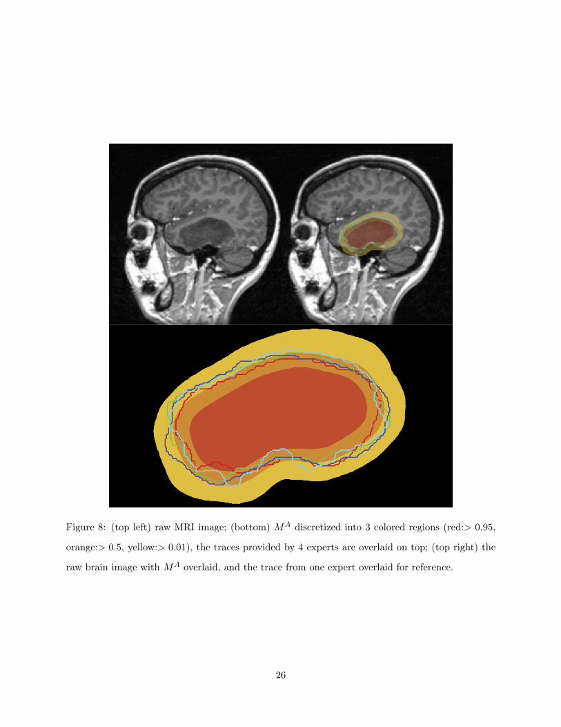
Figure 8: (top left) raw MRI image; (bottom) MA discretized into 3 colored regions (red:> 0.95,

orange:> 0.5, yellow:> 0.01), the traces provided by 4 experts are overlaid on top; (top right) the

raw brain image with MA overlaid, and the trace from one expert overlaid for reference.

26

Aziz, N., Bata, R., and Bhat, S. (2002), “Bezier surface/surface intersection,” Computer Graphics and

Applications, IEEE, 10(1), 50–58.

Barnhill, R. (1985), “Surfaces in computer aided geometric design: A survey with new results,” Computer

Aided Geometric Design, 2(1-3), 1–17.

Bhattacharya, A. (2008), “Statistical analysis on manifolds: A nonparametric approach for inference on

shape spaces,” Sankhya: The Indian Journal of Statistics, 70(Part 3), 0–43.

Bhattacharya, A., and Dunson, D. (2010), “Nonparametric Bayesian density estimation on manifolds with

applications to planar shapes,” Biometrika, 97(4), 851.

Bhattacharya, A., and Dunson, D. (2011a), “Nonparametric Bayes Classification and Hypothesis Testing on

Manifolds,” Journal of Multivariate Analysis, . to appear.

Bhattacharya, A., and Dunson, D. (2011b), “Strong consistency of nonparametric Bayes density estimation

on compact metric spaces,” Annals of the Institute of Statistical Mathematics, . to appear.

Bhattacharya, R., and Bhattacharya, A. (2009), “Statistics on manifolds with applications to shape spaces,”

Publishers page, p. 41.

Bookstein, F. (1986), “Size and shape spaces for landmark data in two dimensions,” Statistical Science,

1(2), 181–222.

Bookstein, F. (1996a), Landmark methods for forms without landmarks: localizing group di↵erences in out-

line shape,, in Mathematical Methods in Biomedical Image Analysis, 1996., Proceedings of the Workshop

on, IEEE, pp. 279–289.

Bookstein, F. (1996b), Shape and the information in medical images: A decade of the morphometric synthe-

sis,, in Mathematical Methods in Biomedical Image Analysis, 1996., Proceedings of the Workshop on,

IEEE, pp. 2–12.

Bookstein, F. (1996c), “Standard formula for the uniform shape component in landmark data,” NATO ASI

SERIES A LIFE SCIENCES, 284, 153–168.

Cinquin, P., Chalmond, B., and Berard, D. (1982), “Hip prosthesis design,” Lecture Notes in Medical Infor-

matics, 16, 195–200.

Desideri, J., Abou El Majd, B., and Janka, A. (2007), “Nested and self-adaptive Bezier parameterizations

for shape optimization,” Journal of Computational Physics, 224(1), 117–131.

27

Desideri, J., and Janka, A. (2004), Multilevel shape parameterization for aerodynamic optimization–

application to drag and noise reduction of transonic/supersonic business jet,, in European Congress

on Computational Methods in Applied Sciences and Engineering (ECCOMAS 2004), E. Heikkola et al

eds., Jyvaskyla, pp. 24–28.

Dryden, I., and Gattone, S. (2001), “Surface shape analysis from MR images,” Proc. Functional and Spatial

Data Analysis, pp. 139–142.

Dryden, I., and Mardia, K. (1993), “Multivariate shape analysis,” Sankhya: The Indian Journal of Statistics,

Series A, pp. 460–480.

Dryden, I., and Mardia, K. (1998), Statistical shape analysis, Vol. 4 John Wiley & Sons New York.

Gong, L., Pathak, S., Haynor, D., Cho, P., and Kim, Y. (2004), “Parametric shape modeling using deformable

superellipses for prostate segmentation,” Medical Imaging, IEEE Transactions on, 23(3), 340–349.

Hagen, H., and Santarelli, P. (1992), Variational design of smooth B-spline surfaces,, in Topics in surface

modeling, Society for Industrial and Applied Mathematics, pp. 85–92.

Hastie, T., and Stuetzle, W. (1989), “Principal curves,” Journal of the American Statistical Association,

pp. 502–516.

Kent, J., Mardia, K., Morris, R., and Aykroyd, R. (2001), “Functional models of growth for landmark data,”

Proceedings in Functional and Spatial Data Analysis, pp. 109–115.

Kume, A., Dryden, I., and Le, H. (2007), “Shape-space smoothing splines for planar landmark data,”

Biometrika, 94(3), 513–528.

Kurtek, S., Srivastava, A., Klassen, E., and Ding, Z. (2011), “Statistical Modeling of Curves Using Shapes

and Related Features,” , .

Lang, J., and Roschel, O. (1992), “Developable (1, n)-Bezier surfaces,” Computer Aided Geometric Design,

9(4), 291–298.

Madi, M. (2004), “Closed-form expressions for the approximation of arclength parameterization for Bezier

curves,” International journal of applied mathematics and computer science, 14(1), 33–42.

Malladi, R., Sethian, J., and Vemuri, B. (1994), “Evolutionary fronts for topology-independent shape mod-

eling and recovery,” Computer VisionECCV’94, pp. 1–13.

Malladi, R., Sethian, J., and Vemuri, B. (1995), “Shape modeling with front propagation: A level set

approach,” Pattern Analysis and Machine Intelligence, IEEE Transactions on, 17(2), 158–175.

28

Mardia, K., and Dryden, I. (1989), “The statistical analysis of shape data,” Biometrika, 76(2), 271–281.

Mokhtarian, F., and Mackworth, A. (1992), “A theory of multiscale, curvature-based shape representation

for planar curves,” IEEE Transactions on Pattern Analysis and Machine Intelligence, 14(8), 789–805.

Mortenson, M. (1985), Geometrie modeling John Wiley, New York.

Muller, H. (2005), Surface reconstruction-an introduction,, in Scientific Visualization Conference, 1997,

IEEE, p. 239.

Pati, D., and Dunson, D. (2011), “Bayesian modeling of closed surfaces through tensor products,” , . (sub-

mitted to Biometrika).

Persoon, E., and Fu, K. (1977), “Shape discrimination using Fourier descriptors,” Systems, Man and Cyber-

netics, IEEE Transactions on, 7(3), 170–179.

Rossi, D., and Willsky, A. (2003), “Reconstruction from projections based on detection and estimation of

objects–Parts I and II: Performance analysis and robustness analysis,” Acoustics, Speech and Signal

Processing, IEEE Transactions on, 32(4), 886–906.

Roth, A., Juhasz, I., Schicho, J., and Ho↵mann, M. (2009), “A cyclic basis for closed curve and surface

modeling,” Computer Aided Geometric Design, 26(5), 528–546.

Sato, Y., Wheeler, M., and Ikeuchi, K. (1997), Object shape and reflectance modeling from observation,,

in Proceedings of the 24th annual conference on Computer graphics and interactive techniques, ACM

Press/Addison-Wesley Publishing Co., pp. 379–387.

Sederberg, T., Gao, P., Wang, G., and Mu, H. (1993), 2-D shape blending: an intrinsic solution to the vertex

path problem,, in Proceedings of the 20th annual conference on Computer graphics and interactive

techniques, ACM, pp. 15–18.

Stepanets, A. (1974), “THE APPROXIMATION OF CERTAIN CLASSES OF DIFFERENTIABLE PERI-

ODIC FUNCTIONS OF TWO VARIABLES BY FOURIER SUMS,” Ukrainian Mathematical Journal,

25(5), 498–506.

Su, B., and Liu, D. (1989), Computational geometry: curve and surface modeling Academic Press Profes-

sional, Inc. San Diego, CA, USA.

Su, J., Dryden, I., Klassen, E., Le, H., and Srivastava, A. (2011), “Fitting Optimal Curves to Time-Indexed,

Noisy Observations of Stochastic Processes on Nonlinear Manifolds,” Journal of Image and Vision

Computing, .

29

van der Vaart, A., and van Zanten, J. (2008), “Reproducing kernel Hilbert spaces of Gaussian priors,” IMS

Collections, 3, 200–222.

Whitney, H. (1937), “On regular closed curves in the plane,” Compositio Math, 4, 276–284.

Zahn, C., and Roskies, R. (1972), “Fourier descriptors for plane closed curves,” Computers, IEEE Transac-

tions on, 100(3), 269–281.

Zheng, Y., John, M., Liao, R., Boese, J., Kirschstein, U., Georgescu, B., Zhou, S., Kempfert, J., Walther,

T., Brockmann, G. et al. (2010), “Automatic aorta segmentation and valve landmark detection in C-

arm CT: application to aortic valve implantation,” Medical Image Computing and Computer-Assisted

Intervention–MICCAI 2010, pp. 476–483.

30