Bayesian Error Propagation for a Kinetic Model of n-Propylbenzene Oxidation in a Shock Tube

Preprint Cambridge Centre for Computational Chemical Engineering ISSN 1473 – 4273

Bayesian Error Propagation for a Kinetic Modelof n-Propylbenzene Oxidation in a Shock Tube

Sebastian Mosbach 1, Je Hyeong Hong 1, George P. E. Brownbridge 1,

Markus Kraft 1, Soumya Gudiyella 2 and Kenneth Brezinsky 3

released: 03 October 2013

1 Department of Chemical Engineeringand BiotechnologyUniversity of CambridgeNew Museums SitePembroke StreetCambridge CB2 3RAUKEmail: mk306@cam.ac.uk

2 Department of Chemical EngineeringUniversity of Illinois at ChicagoChicago, IL 60607USAEmail: sgudiy2@uic.edu

3 Department of Mechanical andIndustrial EngineeringUniversity of Illinois at ChicagoChicago, IL 60607USAEmail: kenbrez@uic.edu

Preprint No. 133

Keywords: n-Propylbenzene, Bayesian parameter estimation, error propagation

Edited by

CoMoGROUP

Computational Modelling GroupDepartment of Chemical Engineering and BiotechnologyUniversity of CambridgeNew Museums SitePembroke StreetCambridge CB2 3RAUnited Kingdom

Fax: + 44 (0)1223 334796E-Mail: c4e@cam.ac.ukWorld Wide Web: http://como.cheng.cam.ac.uk/

Abstract

We apply a Bayesian parameter estimation technique to a chemical kinetic mecha-nism for n-propylbenzene oxidation in a shock tube in order to propagate errors inexperimental data to errors in model parameters and responses. We find that, in or-der to apply the methodology successfully, conventional optimisation is required asa preliminary step. This is carried out in two stages: firstly, a quasi-random globalsearch using a Sobol low-discrepancy sequence is conducted, followed by a localoptimisation by means of a hybrid gradient-descent/Newton iteration method. Theconcentrations of 37 species at a variety of temperatures, pressures, and equivalenceratios are optimised against a total of 2378 experimental observations. We then applythe Bayesian methodology to study the influence of uncertainties in the experimentalmeasurements on some of the Arrhenius parameters in the model as well as someof the predicted species concentrations. Markov Chain Monte Carlo algorithms areemployed to sample from the posterior probability densities, making use of polyno-mial surrogates of higher order fitted to the model responses. We conclude that themethodology provides a useful tool for the analysis of distributions of model param-eters and responses, in particular their uncertainties and correlations. Limitationsof the method are discussed. For example, we find that using second-order responsesurfaces and assuming normal distributions for propagated errors is largely adequate,but not always.

1

Contents

1 Introduction 3

2 Methodology 4

2.1 Experimental data . . . . . . . . . . . . . . . . . . . . . . . . . . . . . . 4

2.2 Shock tube and chemical kinetic model . . . . . . . . . . . . . . . . . . 5

2.3 Sensitivity analysis . . . . . . . . . . . . . . . . . . . . . . . . . . . . . 5

2.4 Global search and local optimisation . . . . . . . . . . . . . . . . . . . . 6

2.5 Bayesian parameter estimation . . . . . . . . . . . . . . . . . . . . . . . 7

2.5.1 Bayes’ Theorem . . . . . . . . . . . . . . . . . . . . . . . . . . 7

2.5.2 Likelihood . . . . . . . . . . . . . . . . . . . . . . . . . . . . . 8

2.5.3 Prior distributions . . . . . . . . . . . . . . . . . . . . . . . . . . 8

2.5.4 Posterior distributions . . . . . . . . . . . . . . . . . . . . . . . 8

2.5.5 Markov Chain Monte Carlo sampling . . . . . . . . . . . . . . . 9

3 Results 9

3.1 Sensitivity analysis . . . . . . . . . . . . . . . . . . . . . . . . . . . . . 9

3.2 Global search and local optimisation . . . . . . . . . . . . . . . . . . . . 9

3.3 Bayesian parameter estimation and error propagation . . . . . . . . . . . 19

4 Conclusions 21

References 22

2

1 Introduction

The quantification of uncertainties in experimental as well as computational data has longbeen recognised as essential across all areas of science and technology. The field ofcombustion modelling is no exception [20, 58]. It is well-established [49, 72] that makingchemical models reliable and predictive requires calculation results to be accompanied byuncertainty bounds – with greater predictive power corresponding to smaller error bounds.

Various techniques for uncertainty quantification and propagation have been used in com-bustion kinetic modelling. An elementary way to relate uncertainties in model parametersto uncertainties in model outputs is via local sensitivity coefficients [62, 65]. The sameidea can be extended to global sensitivities in order to be able to treat strong model non-linearities combined with large uncertainties [57, 73]. For example, global sensitivitymethods have been used to propagate uncertainties from parameters in first-principlescalculations to reaction rate coefficients [23]. Uncertainties of the three parameters in theArrhenius rate law, with particular emphasis on their joint distribution and its temperaturedependence, have been investigated in detail [40, 41, 66, 67]. Given that error propa-gation is intrinsically part of parameter estimation, frequently in the sense of optimisingwith respect to an objective function in one form or another, it is also natural to considerconfidence regions defined by the contours of the objective function surface [21, 37].

In the Data Collaboration framework [20, 49, 51, 72], uncertainties are specified throughdeterministic upper and lower bounds rather than probability distributions. It employsoptimisation techniques in conjunction with solution mapping [21] in order to quantifyprediction uncertainties [22], rigorously measure data set consistency [16], quantitativelydiscriminate between multiple candidate models [17], and to conduct sensitivity analy-ses of uncertainties in responses with respect to experimental errors and uncertainties inmodel parameters [48].

Spectral uncertainty quantification is a technique based on polynomial chaos expansions[69, 70], in which uncertain quantities, such as model parameters, are represented as se-ries of basis random variables. The essence of the method consists in determining thecoefficients of the expansion, the spectral modes, which can be used to reconstruct theprobability density, at least to the finite order of the truncated series. The spectral methodhas been introduced to combustion research, specifically in the areas of reacting flowsand chemical kinetics, in the form of a post-processing step to conventional Monte Carloanalysis [45–47] in which the spectral modes are determined. The technique has beenadapted, using quadratic response surfaces, to derive an analytic expression for the vari-ance of model responses and combined with optimisation such that experimental errorscan be propagated simultaneously into rate coefficients and their uncertainties [52–54].

Bayesian methods are based on a systematic probability-theoretic treatment of all involvedquantities including in particular experimental data as well as model parameters, and cen-tre around applying Bayes’ theorem to update knowledge represented in the form of dis-tributions [4]. Bayesian methods have been used in chemical kinetics for at least half acentury [2], but their popularity in this and other fields [1] has increased significantly inrecent years due to an influential paper by Kennedy and O’Hagan [30]. In particular, theuse of Markov Chain Monte Carlo (MCMC) sampling has become wide-spread, at least

3

to some extent as a consequence of readily available powerful computers. For example,Bayesian uncertainty quantification using MCMC has been applied to rate coefficients ofsingle reactions, such as H+O2→OH+O using shock tube data [36], and hydrogen ab-straction from isopropanol using ab initio calculations [43]. The same methods, as wellas polynomial chaos expansions, have also been employed for quantifying uncertaintiesin entire reaction mechanisms, focusing specifically on correlations between the three pa-rameters in the Arrhenius law [42]. Bayesian parameter estimation also naturally extendsto and is closely related to experimental design [27, 28, 39]. Although Bayesian tech-niques are not new as such, and some applications exist, there continues to be a need forcase studies which demonstrate the performance of the methods.

The purpose of this paper is to apply a Bayesian method for parameter estimation and er-ror propagation as a case study to a detailed chemical kinetic model for n-propylbenzeneoxidation in a shock tube and report on the experience gained with the method. n-propylbenzene has been suggested as a potential surrogate for the alkylbenzene classof components of commercial aviation fuels [10, 14]. The kinetic model contains 191species and 1127 reactions. Prior to using Bayesian methods, for reasons explained be-low, we perform optimisation with conventional techniques. We conduct a quasi-randomglobal search in a parameter space spanned by 64 Arrhenius pre-exponential factors, se-lected by means of sensitivity analysis, and then use a set of best points found to initiatelocal gradient-descent optimisation from those points. A standard least-squares objectivefunction weighted by experimental errors is utilised to assess agreement with experimen-tal data, which comprise of 2378 individual observations of 37 species concentrationsat 74 different experimental process conditions with varying pressure, temperature, andequivalence ratio. For the best point resulting from the optimisation, we apply Bayesianparameter estimation for a small number of parameters, and use an MCMC method to ob-tain posterior probability densities. For this purpose, we fit a surrogate model that consistsof polynomials of various orders to the responses. We discuss strengths and weaknessesof the method.

2 Methodology

In this section, we briefly describe the experimental data set and combustion model usedin this work, and give details of each of the steps involved in performing the error prop-agation, namely, sensitivity analysis, global search, local optimisation, and Bayesian pa-rameter estimation.

2.1 Experimental data

The data set we consider here [24] was obtained using the high-pressure single-pulseshock tube at the University of Illinois at Chicago [56, 61]. Process condition variablescomprise of initial temperature, initial pressure, initial composition, and reaction time.In all cases, the initial mixture is composed of n-propylbenzene, oxygen, and argon.The mixture is highly diluted, with an n-propylbenzene mole fraction of about 90 ppm

4

throughout, so the system can be considered isothermal to a good approximation. Anoverview of the conditions is given in Table 1.

Table 1: Overview of experimental process conditions.

Average shock Temperature Fuel mole Reaction timepressure [atm] range [K] fraction [ppm] Φ range [ms]

28 907-1551 86 0.54 1.40-2.0551 959-1558 90 0.55 1.27-1.9049 838-1635 90 1.0 1.21-1.9524 905-1669 89 1.9 1.36-2.9352 847-1640 90 1.9 1.26-1.95

Species concentrations were determined by means of gas chromatography in gases sam-pled from the shock tube. Measured species include O2, CO, CO2, aliphatic hydrocar-bons such as methane, ethane, propane, acetylene, ethene, propene, propadiene, propyne,1,3-butadiene, 1,2-butadiene, 2-butyne, vinylacetylene, diacetylene, and cyclopentadi-ene, aromatic hydrocarbons such as benzene, toluene, phenylacetylene, styrene, ethyl-benzene, 1-propenylbenzene, 2-propenylbenzene, n-propylbenzene, indene, naphthalene,2-ethynylnaphthalene, bibenzyl, diphenylmethane, stilbene, fluorene, and anthracene, andthe oxygenated aromatics phenol, benzylalcohol, benzaldehyde, and benzofuran. Mea-surement errors are given for each species and range between 1.7% and 25%, with anaverage of about 12%.

In total, there are 2378 experimental observations of 37 species across 74 points in process-condition space. The complete data set is available online as supplementary material to aprevious publication [24].

2.2 Shock tube and chemical kinetic model

The shock tube is modelled as a homogeneous, adiabatic, constant pressure reactor. Thecorresponding governing equations are standard and shall not be repeated here. As soft-ware to solve the equations, kinetics v8.0 [9] was employed.

As chemical kinetic model, a mechanism developed previously [24], extending earlierwork [11, 32], was used. It contains 191 species and 1127 reactions. All species men-tioned in subsection 2.1 are present in the mechanism.

2.3 Sensitivity analysis

As it is neither feasible nor necessary to tune all kinetic parameters present in a reactionmechanism simultaneously, a subset needs to be chosen. It is natural to use sensitivityanalysis for this [37, 44, 59, 62, 64, 65]. The basic idea is to calculate the normalised

5

sensitivity coefficients of chosen responses with respect to all Arrhenius pre-exponentialfactors and then rank the reactions according to the modulus of their coefficients.

The normalised sensitivity coefficient of the ith response ηi (evaluated at a particular pointξ in process condition space) with respect to the j th model parameter θj is defined by

θjηi(ξ, θ)

∂ηi(ξ, θ)

∂θj.

One way to determine these coefficients is through a finite difference approximation [44,62, 65]. If we denote the vector of model parameters perturbed in the j th direction by

θj := (θ1, . . . , θj−1, (1 + r)× θj, θj+1, . . . , θn),

where r is a (small, positive) number representing a relative perturbation, then this can bewritten as

θjηi(ξ, θ)

ηi(ξ, θj)− ηi(ξ, θ)

(θj − θ)j=ηi(ξ, θ

j)− ηi(ξ, θ)rηi(ξ, θ)

. (1)

Now, the present data set has been obtained at numerous points ξ(1), . . . , ξ(Np.c.) in processcondition space. We find that the sensitivity coefficients, of any particular response withrespect to any particular parameter, vary considerably between these points. There aretwo contributions to this: the parametric derivative, and the value of the response. If thevalue of the response approaches zero, which is common in this data set, the sensitivitycoefficient can become unduly large, in some circumstances amplifying numerical noiseto an extent that it becomes dominant. For this reason, we normalise not by the localvalue ηi(ξ(n), θ) of the response, but by its maximum value maxn{ηi(ξ(n), θ)} across allpoints in process condition space. It is then possible to compare the resulting coefficientsbetween different process conditions. More on the subject of dependence of sensitivitieson process conditions can be found for example in [75]. Thus, instead of (1) we consider

Sij :=maxn

{|ηi(ξ(n), θj)− ηi(ξ(n), θ)|

}rmaxn

{ηi(ξ(n), θ)

} . (2)

In order to obtain a single quantity which can be applied to ranking the reactions we usethe largest value maxi{Sij} among the responses.

We note that this analysis is local in parameter space but global in process condition spacein the sense that sensitivities at every considered point in process condition space are takeninto account.

2.4 Global search and local optimisation

In order to quantify agreement between experiment and model, we use the least-squaresobjective function

Φ(θ) =74∑n=1

∑responses i

[ηi(ξ(n), θ)− ηexpi (ξ(n))

σ(n)i

]2, (3)

6

where n indexes the points in process condition space. For the weights σ(n)i of the in-

dividual terms, we choose the maximum value of each response within each of the fivesets of points in process condition space, multiplied by twice the percentage experimentalerror. The maximum is chosen rather than individual values since, by reasoning similarto the previous subsection, most responses approach zero in every set, and these pointswould receive a dominant weight within each set, leading to counter-intuitive results. Weapply this for each set separately rather than for the entire collection of points in processcondition space as the magnitude of some of the responses can vary considerably from setto set, with equivalence ratio in particular.

Optimisation of the above objective function is carried out in two stages, namely a quasi-random global search as first stage, followed by a local optimisation as second stage.For the global search, a Sobol low-discrepancy sequence [55] is employed. For the localoptimisation, an implementation of the Levenberg-Marquardt [31, 34] method, which is ahybrid between a gradient-descent method and a Newton iteration, is used.

Extensive work has been carried out on uncertainty bounds of Arrhenius parameters [40,41, 67], feasible sets in such parameter spaces [16, 22, 49, 71], and optimisation of pa-rameters beyond the basic Arrhenius ones, such as third-body efficiencies [13]. However,in order to explore the performance of the Bayesian methodology for parameter estima-tion and error propagation, which is the principal aim of this paper, it is sufficient to findany local minimum with respect to whichever parameters are considered. Therefore, forsimplicity, we restrict ourselves in the present work to pre-exponential factors within a hy-percube. We find that optimisation is necessary, though, as direct application of Bayesianmethods to the original, unoptimised mechanism proved to be too problematic mainly re-garding surrogate fidelity over sufficiently wide ranges in parameter space. We point outthat the global search and local gradient-based optimisation in this work are conductedusing the actual model, rather than a surrogate.

2.5 Bayesian parameter estimation

In this section, we briefly summarise the Bayesian methodology [1, 30] which we haveapplied previously in a different context [29, 39], and extend the formulation to het-eroskedastic. This further builds upon our earlier work on parameter estimation and un-certainty propagation in the areas of granulation [5–7, 33] and combustion [50].

2.5.1 Bayes’ Theorem

The current knowledge about the values of the model parameters θ can be represented by aprobability density p(θ), called the prior distribution. When additional experimental datais obtained, represented as a probability density p(ηexp|θ), then the knowledge about themodel parameters can be updated, resulting in a posterior distribution p(θ|ηexp). Bayes’Theorem states how the posterior can be calculated:

p(θ|ηexp) ∝ p(ηexp|θ)p(θ),

7

or in words, ‘Posterior∝ Likelihood× Prior’. In order to estimate the values of the modelparameters using the posterior distribution, likelihood and prior need to be specified.

2.5.2 Likelihood

For the likelihood, i.e. the distribution of the experimental responses, we assume a Gaus-sian centred at the model response:

ηexp,(n) = η(ξ(n), θ

)+ ε(n) with ε(n) ∼ NL(0,Σ(n)), (4)

where ε(n) is the vector of the measurement errors which are normally distributed withzero mean and covariance matrix Σ(n), and L denotes the total number of responses. Thecovariance matrix Σ(n) of the experimental errors is allowed to vary from point to pointin process condition space, i.e. the system can be heteroskedastic. We note here that (4)does not include a model inadequacy term, which accounts for any systematic discrepancybetween experiment and model [8, 26, 30].

Equation (4) implies that, as ηexp,(n) ∼ NL(η(ξ(n), θ),Σ(n)

), the probability density of

observing a particular response ηexp,(n) in the nth experiment is given by

p(ηexp,(n)

∣∣θ,Σ(n))

= (2π)−L/2(

det Σ(n))−1/2

exp(− 1

2ε(n)

>(Σ(n)

)−1ε(n)),

and hence, assuming independent experiments, the likelihood becomes

p(ηexp,(1), . . . , ηexp,(N)

∣∣θ,Σ(1), . . . ,Σ(N))

=

= (2π)−NL/2[ N∏j=1

(det Σ(j))−1/2]

exp

(− 1

2

N∑n=1

ε(n)>(

Σ(n))−1

ε(n)).

2.5.3 Prior distributions

For the prior of θ, we consider a constant, i.e. uniform, distribution over a hypercube Cwhich is defined as the region in P -dimensional space such that θj ∈ [−1, 1] for allj = 1, . . . , P . This gives as prior probability density p(θ) = |C|−11{θ∈C}, where | · |denotes the volume of a set and 1{·} is the indicator function.

2.5.4 Posterior distributions

The posterior density for θ can now be obtained from Bayes’ Theorem as

p(θ∣∣ηexp,(1), . . . , ηexp,(N)

)∝ exp

(− 1

2

N∑n=1

ε(n)>(

Σ(n))−1

ε(n))· 1{θ∈C}. (5)

8

2.5.5 Markov Chain Monte Carlo sampling

In order to derive useful information about the unknown parameters from the posteriordensity (5), we employ the Markov Chain Monte Carlo sampling algorithms of Metropolis-Hastings [25, 35] and Wang-Landau [68]. The collection of samples can be used to plot(marginal) distributions and obtain quantities such as ‘best’ parameter estimates, i.e. thepoints of highest probability density, and high probability density regions, whose boundscan serve as error bars.

The large numbers of samples typically required by these types of algorithm render thedirect use of the model infeasible due to computational expense. For this reason, surrogatemodels are widely used in this situation. Examples for the use of such models in the fieldof combustion include quadratic response surfaces [15, 18, 19, 21, 37, 39, 60], third orderpolynomials [12], higher order orthonormal polynomials [63], cubic natural splines [38],and High-Dimensional Model Representation (HDMR) [74]. We use polynomials of ar-bitrary order in this work.

3 Results

3.1 Sensitivity analysis

As described in subsection 2.3, we conduct a sensitivity analysis of all 37 responses withrespect to the Arrhenius pre-exponential factors of all of the 1127 reactions, across allof the 74 points in process condition space, through finite differencing. This simulationinvolves 74 × (1 + 1127) = 83472 model evaluations. We find that using a relativeperturbation of r = 1% (see Eqn. (2)) represents a good trade-off between avoiding bothrounding error issues and the onset of non-linearities in the model responses. This agreeswith recommendations in the literature [65]. The coefficients, with their sign restored,are shown in Fig. 1 for the 64 most sensitive reactions. We find that the obtained rankingdiffers appreciably, though not substantially, from those carried out at single points inprocess condition space for individual responses [24].

3.2 Global search and local optimisation

We arbitrarily choose to include all of the reactions listed in Fig. 1 into this step. For eachof the reactions, we define the lower and upper bounds of the Arrhenius pre-exponentialfactor to be given by the nominal value divided and multiplied by 5 respectively. Weevaluate 104 points of a Sobol sequence, involving 7.4 × 105 model evaluations, in thishypercube.

We then run Levenberg-Marquardt optimisations starting from some of the best points, i.e.those with lowest objective function value. Due to the random nature of the global search,and the extreme sparsity of the points in high dimensions, it is advisable to consider notjust one but several of the best points, as the best point found in the global search doesnot guarantee the best result overall after further optimisation. All results shown in the

9

-2.5 -2 -1.5 -1 -0.5 0 0.5 1

R___1: H+O2<=>O+OHR1116: C6H5CH2C6H5=FLUORENE+H2R1115: C6H5+C6H5CH2=C6H5CH2C6H5R_148: C3H8(+M)<=>CH3+C2H5(+M)R1022: BPHC3H6=C6H5C3H5+HR_818: C6H5O+H(+M)=C6H5OH(+M)R_589: C6H5CH2+OH=C6H5CH2OHR_859: C5H5+OH=C4H6-13+COR_989: PHC3H7=C6H5CH2+C2H5R_340: C2H2+CH3<=>PC3H4+HR_555: C6H5CH3(+M)=C6H5CH2+H(+M)R1012: BPHC3H6=C6H5C3H5-2+HR1124: C6H5CH2+CO=>C8H6O+HR1096: INDENYL+C5H5=>A3+2HR_793: C6H5+O2=C6H5OOR_152: H+C2H4(+M)<=>C2H5(+M)R1013: BPHC3H6=C6H6+AC3H5R1006: PHC3H7+OH=CPHC3H6+H2OR_616: C14H14+OH=C14H13+H2OR1058: INDENE+H=INDENYL+H2R1087: A2+C2H=A2C2H+HR1000: PHC3H7+OH=BPHC3H6+H2OR_998: PHC3H7+H=BPHC3H6+H2R1071: 2C5H5=>A2+2HR_592: C6H5CH2+CH3=C6H5C2H5R__35: CH3+CH3(+M)<=>C2H6(+M)R__13: HO2+OH<=>H2O+O2R_155: C2H4+O<=>CH3+HCOR_839: C5H5+H(+M)=C5H6(+M)R_591: C6H5CH2+HO2=C6H5CH2O+OHR__25: CO+OH<=>CO2+HR_585: C6H5CH2=C5H5+C2H2R1057: INDENE=INDENYL+HR_162: C4H6-13+H<=>C2H4+C2H3R_282: AC3H5+H(+M)<=>C3H6(+M)R1052: C6H5C2H+H=C6H5+C2H2R_357: H2CCCH+CH3(+M)<=>C4H6-12(+M)R1125: C6H5CH2+HCO=>C8H6O+H2R__54: HCO+M=H+CO+MR_820: C6H5O=CO+C5H5R_587: C6H5CH2+O=C6H5CHO+HR_388: C4H4+OH<=>C4H3-I+H2OR_768: C6H5C2H3+OH=C6H5CCH2+H2OR__31: CH3+H(+M)<=>CH4(+M)R_390: C4H4+H<=>C4H5-NR_655: C6H5CHO+OH=C6H5CO+H2OR_321: AC3H4+H<=>AC3H5R_992: PHC3H7+H=APHC3H6+H2R_844: C5H6+H=C5H5+H2R_653: C6H5CHO+H=C6H5CO+H2R_134: C2H6+OH<=>C2H5+H2OR_791: C6H5+O2=C6H5O+OR1127: C6H5O+C6H5O=DIBZFUR+H2OR_981: HCCO+O2=HCO+CO+OR_588: C6H5CH2+O=C6H5+CH2OR_507: C4H6-12<=>C4H6-13R_535: C4H5-N+O2<=>CH2CHCHCHO+OR1040: C6H5C3H5+H=C6H5CH2+C2H4R1105: A3+OH=>A2C2H+CH2CO+HR1093: INDENYL+H2CCCH=>A2C2H+2HR_804: C6H5OH+OH=C6H5O+H2OR_387: C4H4+OH<=>C4H3-N+H2OR1118: OH+FLUORENE=>P2+CO+HR_176: C2H2+O<=>HCCO+H

Normalised sensitivity coefficient

Figure 1: Normalised sensitivity coefficients for the 64 most sensitive reactions across allconsidered points in process condition space.

10

Table 2: Square roots of the ratios of partial sums of objective function terms for theoptimised and original mechanisms. The majority of contributions has improved(highlighted).

Average pressure [atm]: 28 51 49 24 52Equivalence ratio Φ: 0.54 0.55 1.0 1.9 1.9

n-Propylbenzene 1.378 1.419 4.808 1.015 0.969O2 1.052 0.651 0.654 0.128 0.211

CO 0.421 0.403 0.660 0.257 0.274CO2 0.405 0.138 0.224 0.236 0.302

Methane 2.130 2.885 0.889 0.645 0.868Ethene 0.663 1.984 0.903 0.356 0.403Ethane 1.875 2.375 1.809 1.214 0.728

Acetylene 1.057 1.048 1.380 1.156 1.125Propadiene 0.777 3.582 1.898 0.437 0.510

Propyne 0.730 0.494 1.018 0.708 0.457Vinylacetylene 0.735 0.764 0.813 0.776 0.580

Diacetylene 0.464 0.445 0.140 0.615 0.324Benzene 0.915 0.855 1.077 0.897 0.737Toluene 1.395 1.355 1.004 0.245 0.361

Phenylacetylene 0.076 0.170 0.349 0.139 0.168Styrene 0.415 1.554 0.747 0.452 0.927

Cyclopentadiene 0.292 0.433 0.342 0.889 0.632Ethylbenzene 0.481 0.252 0.333 0.360 0.244Benzaldehyde 1.989 5.544 5.334 0.277 0.346

Phenol 0.151 0.775 0.078 0.133 0.1151-Propenylbenzene 0.048 0.027 0.042 0.148 0.028

Indene 1.077 1.107 1.190 1.625 1.291Naphthalene 0.630 0.598 0.806 1.083 0.995

1,3-Butadiene 0.902 1.236 0.688 0.191 0.281Bibenzyl 0.927 1.134 0.560 0.722 0.759

Benzofuran 0.957 0.976 0.960 0.931 0.926Diphenylmethane 0.570 0.833 0.581 0.637 0.627

Propane 0.737 0.690 0.5981,2-Butadiene 0.941

2-Butyne 0.8362-Propenylbenzene 0.019 0.108

Benzylalcohol 0.797 0.7842-Ethynylnaphthalene 0.676 0.669 0.929 0.922

Fluorene 0.989 0.870 1.152Stilbene 0.428 0.554 0.505

Anthracene 0.277 0.381 0.250Propene 4.480 3.185

11

Temperature [K]

n−P

ropy

lben

zene

mol

e fr

actio

n [p

pm]

● ●●

●

●

●

●

● ●● ● ● ● ● ●

● ● ● ●

●

●

● ● ●●● ● ●● ●

1000 1200 1400 1600

020

4060

8010

0

●ExperimentModel (original)Model (orig., avg.)Model (optimised)Model (opt., avg.)

(a) n-Propylbenzene (averagepressure 49 atm, Φ = 1.0).

Temperature [K]

O2

mol

e fr

actio

n [p

pm]

●●●

●● ● ●

●●

● ●

●

●

●

●

●

● ●● ●● ● ● ●● ●●

●

●

●

●

●

1000 1200 1400 1600

010

020

030

040

050

060

0

●ExperimentModel (original)Model (orig., avg.)Model (optimised)Model (opt., avg.)

(b) O2 (average pressure 24 atm,Φ = 1.9).

Temperature [K]

CO

mol

e fr

actio

n [p

pm]

● ●● ●● ● ● ●●

● ●

●

●

●

●

●

● ●● ●● ● ● ● ● ●●●

●

●

●

●

1000 1200 1400 1600

020

040

060

0

●ExperimentModel (original)Model (orig., avg.)Model (optimised)Model (opt., avg.)

(c) CO (average pressure 24 atm,Φ = 1.9).

Temperature [K]

CO

2 m

ole

frac

tion

[ppm

]

● ● ● ● ●

●

●

●

●●

● ● ● ● ● ●

●

●

●

●

1000 1200 1400

020

040

060

080

0 ●ExperimentModel (original)Model (orig., avg.)Model (optimised)Model (opt., avg.)

(d) CO2 (average pressure 51 atm,Φ = 0.55).

Temperature [K]

Ace

tyle

ne m

ole

frac

tion

[ppm

]

● ●●

●

●

●

●

●

●

●

● ●● ● ● ●● ● ● ●

●

●

●

●

●

● ● ●● ● ● ●

1000 1200 1400

05

1015

2025

●ExperimentModel (original)Model (orig., avg.)Model (optimised)Model (opt., avg.)

(e) Acetylene (average pressure28 atm, Φ = 0.54).

Temperature [K]

Pro

pyne

mol

e fr

actio

n [p

pm]

● ● ● ●

●

●

●

● ● ●● ● ● ●

●

●

●

● ● ●

1000 1200 1400

0.0

0.5

1.0

1.5

2.0

●ExperimentModel (original)Model (orig., avg.)Model (optimised)Model (opt., avg.)

(f) Propyne (average pressure51 atm, Φ = 0.55).

Temperature [K]

Vin

ylac

etyl

ene

mol

e fr

actio

n [p

pm]

● ● ● ● ●

●

●

●

●

●

●

●

●

●

●

● ●● ● ● ● ●● ●

●

●●

●

●

●●

●

●

●

1000 1200 1400 1600

0.0

0.5

1.0

1.5

2.0

2.5 ●

ExperimentModel (original)Model (orig., avg.)Model (optimised)Model (opt., avg.)

(g) Vinylacetylene (average pres-sure 52 atm, Φ = 1.9).

Temperature [K]

Dia

cety

lene

mol

e fr

actio

n [p

pm]

● ● ● ● ● ●

●

●

●

●

●

● ● ● ●● ● ● ● ● ●●

●

●

●

●

●

●● ●

1000 1200 1400 1600

0.0

0.5

1.0

1.5 ●

ExperimentModel (original)Model (orig., avg.)Model (optimised)Model (opt., avg.)

(h) Diacetylene (average pressure49 atm, Φ = 1.0).

Temperature [K]

1,3−

But

adie

ne m

ole

frac

tion

[ppm

]

● ●● ●● ●●

●

●

●

●

●

●

● ●●● ●● ●● ● ●

●

●

●

●

●

●

●

●

●

1000 1200 1400 1600

0.0

0.5

1.0

1.5

2.0

●ExperimentModel (original)Model (orig., avg.)Model (optimised)Model (opt., avg.)

(i) 1,3-Butadiene (average pres-sure 24 atm, Φ = 1.9).

Figure 2: Comparison of selected responses of the original as well as the optimised modelwith experiment. Each graph corresponds to an entry in Table 2.

12

Temperature [K]

Ben

zene

mol

e fr

actio

n [p

pm]

● ● ● ●

●

●

●

●

●

●

●

●

●

●

● ● ●● ● ● ●●

●

●

●

●●

●

● ●●

●

●

●

1000 1200 1400 1600

05

1015

20

●ExperimentModel (original)Model (orig., avg.)Model (optimised)Model (opt., avg.)

(a) Benzene (average pressure52 atm, Φ = 1.9).

Temperature [K]

Tolu

ene

mol

e fr

actio

n [p

pm]

● ●● ●● ●

●

●

●

● ●

●

●

● ● ●● ●● ●● ●●

●

●

●

●●

●

●

● ●

1000 1200 1400 1600

010

2030

4050

●ExperimentModel (original)Model (orig., avg.)Model (optimised)Model (opt., avg.)

(b) Toluene (average pressure24 atm, Φ = 1.9).

Temperature [K]

Ben

zald

ehyd

e m

ole

frac

tion

[ppm

]

● ● ● ●

●

●

●

●

●

●

● ●●

● ●● ● ●●

●

●

●

●

●●

●● ●● ●

1000 1200 1400 1600

02

46

810

●ExperimentModel (original)Model (orig., avg.)Model (optimised)Model (opt., avg.)

(c) Benzaldehyde (average pres-sure 49 atm, Φ = 1.0).

Temperature [K]

Phe

nol m

ole

frac

tion

[ppm

]

● ● ● ●

●

●

●

●

●● ● ● ● ● ●● ● ● ●

●

●

●

●

●

●

●

●●● ●

1000 1200 1400 1600

01

23

45

6

●ExperimentModel (original)Model (orig., avg.)Model (optimised)Model (opt., avg.)

(d) Phenol (average pressure49 atm, Φ = 1.0).

Temperature [K]

1−P

rope

nylb

enze

ne m

ole

frac

tion

[ppm

]

● ● ● ●

●

●

●

●●

●

●●

●● ● ● ●● ● ●

●

●

●

●

●

●

●

●

●

●● ● ● ●

1000 1200 1400 1600

0.0

0.2

0.4

0.6

0.8

1.0

●ExperimentModel (original)Model (orig., avg.)Model (optimised)Model (opt., avg.)

(e) 1-Propenylbenzene (averagepressure 52 atm, Φ = 1.9).

Temperature [K]

2−P

rope

nylb

enze

ne m

ole

frac

tion

[ppm

]

● ●● ●● ●● ● ● ● ● ● ● ● ● ●● ●● ●●

●

●

●●

●

●

●

●

● ● ●

1000 1200 1400 1600

01

23

45

6

●ExperimentModel (original)Model (orig., avg.)Model (optimised)Model (opt., avg.)

(f) 2-Propenylbenzene (averagepressure 24 atm, Φ = 1.9).

Temperature [K]

Phe

nyla

cety

lene

mol

e fr

actio

n [p

pm]

● ●

●●

●

●

●

●

● ● ● ● ● ● ● ●● ● ●

●

●

●

●

●

●

●

●●

● ● ● ●

1000 1200 1400

01

23

45

67

●ExperimentModel (original)Model (orig., avg.)Model (optimised)Model (opt., avg.)

(g) Phenylacetylene (averagepressure 28 atm, Φ = 0.54).

Temperature [K]

Inde

ne m

ole

frac

tion

[ppm

]

● ●● ●● ●

●

●

●

●

●

●

●

● ● ●● ●● ●● ●●

●

●

●

● ●

●

●

●

●

1000 1200 1400 1600

0.0

0.2

0.4

0.6

0.8

1.0

●ExperimentModel (original)Model (orig., avg.)Model (optimised)Model (opt., avg.)

(h) Indene (average pressure24 atm, Φ = 1.9).

Temperature [K]

Nap

htha

lene

mol

e fr

actio

n [p

pm]

● ● ●

●

●●

●

● ● ●● ● ● ● ●

●

●

●

● ●

1000 1200 1400

0.0

0.1

0.2

0.3

0.4

0.5

0.6

0.7

●ExperimentModel (original)Model (orig., avg.)Model (optimised)Model (opt., avg.)

(i) Naphthalene (average pressure51 atm, Φ = 0.55).

Figure 3: Comparison of selected responses of the original as well as the optimised modelwith experiment. Each graph corresponds to an entry in Table 2.

13

A' 1

006

−1.

0−

0.5

0.0

0.5

1.0

A' 1

022

−1.

0−

0.5

0.0

0.5

1.0

A' 5

55−

1.0

−0.

50.

00.

51.

0

A'989

A' 5

92

−1.0 −0.5 0.0 0.5 1.0

−1.

0−

0.5

0.0

0.5

1.0

A'1006

−1.0 −0.5 0.0 0.5 1.0

A'1022

−1.0 −0.5 0.0 0.5 1.0

A'555

−1.0 −0.5 0.0 0.5 1.0

Figure 4: Marginal posterior densities for selected pre-exponential factors. Their shapeis Gaussian to a good approximation.

14

Tolu

ene

[ppm

]15

2025

3035

Inde

ne [p

pm]

0.15

0.25

0.35

A2

[ppm

]1.

101.

20

Benzene [ppm]

A3

[ppm

]

6.5 7.0 7.5 8.0

0.01

00.

020

Toluene [ppm]15 20 25 30 35

Indene [ppm]0.15 0.25 0.35

A2 [ppm]1.10 1.20

Figure 5: Marginal posterior densities for selected responses at an average pressure of52 atm, Φ = 1.9, T = 1286 K.

15

T=

1173

K2.

53.

03.

54.

0T

=12

86 K

6.5

7.0

7.5

8.0

T=

1449

K5

67

8

T=1041 K

T=

1527

K

0.15 0.25 0.35

2.4

2.6

2.8

3.0

3.2

T=1173 K2.5 3.0 3.5 4.0

T=1286 K6.5 7.0 7.5 8.0

T=1449 K5 6 7 8

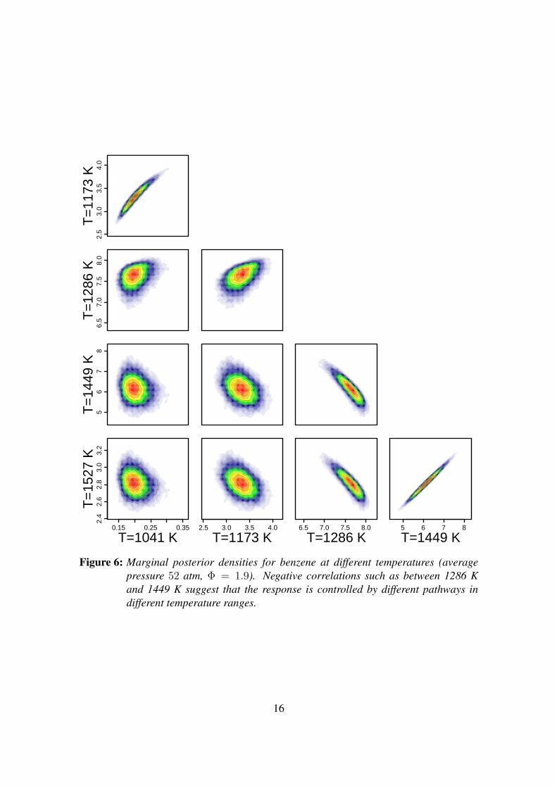
Figure 6: Marginal posterior densities for benzene at different temperatures (averagepressure 52 atm, Φ = 1.9). Negative correlations such as between 1286 Kand 1449 K suggest that the response is controlled by different pathways indifferent temperature ranges.

16

Temperature [K]

Benz

ene

mol

e fr

actio

n [p

pm]

1000 1200 1400 1600

05

1015

20ExperimentModel (optimised)Model (opt., avg.)

cde

fg

h

(a) Benzene.

Temperature [K]

Tolu

ene

mol

e fr

actio

n [p

pm]

1000 1200 1400 1600

05

1015

2025

30

ExperimentModel (optimised)Model (opt., avg.)

cd

e

f

g

h

(b) Toluene.

Benzene [ppm]

Tolu

ene

[ppm

]

4.8 5.0 5.2 5.4 5.6 5.8 6.0

1520

2530

(c) T = 1228 K.Benzene [ppm]

Tolu

ene

[ppm

]

5.5 6.0 6.5 7.0

1520

2530

35

(d) T = 1263 K.Benzene [ppm]

Tolu

ene

[ppm

]

6.5 7.0 7.5 8.0

1520

2530

35

(e) T = 1286 K.

Benzene [ppm]

Tolu

ene

[ppm

]

9.8 10.0 10.4 10.8 11.2

1015

2025

(f) T = 1374 K.Benzene [ppm]

Tolu

ene

[ppm

]

8 9 10 11

46

810

1214

16

(g) T = 1419 K.Benzene [ppm]

Tolu

ene

[ppm

]

5 6 7 80.5

1.0

1.5

2.0

2.5

3.0

3.5

(h) T = 1449 K.

Figure 7: Correlations between benzene and toluene mole fractions at different temper-atures (average pressure 52 atm, Φ = 1.9). As the temperature increases, thecorrelation becomes stronger and turns from negative to positive. The errorbars for the model response in Figs. 7a and 7b are the 2σ HPD regions derivedfrom the one-dimensional marginal distributions.

17

following are for the best point overall which was found with the Levenberg-Marquardtoptimisation run initiated from the second-best Sobol point.

In order to assess in more detail the improvement or deterioration of the agreement be-tween experiment and model, we consider the partial sums of those terms in the objectivefunction (3) belonging to each species and each of the five sets of conditions as sum-marised in Table 1. Table 2 lists, for each measured species and for each of the five setsof conditions, the square root of the ratios of the value of the corresponding partial sumfor the optimised mechanism and the original one. Ratios less than one, i.e where theagreement has improved, are highlighted. Most of the contributions – 120 out of 159,more than 75% – have improved.

Figures 2 and 3 show a comparison of selected responses of the original as well as theoptimised model with experiment. Each model data point displayed is evaluated at itsexact condition, i.e. at the experimental pressure and reaction time, whereas the curveslabelled ‘average’ are temperature sweeps evaluated at an average pressure and reactiontime. The average curves, included as a visual aid but also because they were used inprevious work [24], differ somewhat from the values obtained at the exact conditionsmainly due to the fact that many species concentrations change significantly over theobserved time-scale. Each graph in these figures corresponds to an entry in Table 2. Forexample, for O2 at an average pressure of 24 atm and and equivalence ratio of 1.9 (Fig. 2b),the sum of those terms in the objective function corresponding to the data points in thegraph has decreased by a factor of 0.128−2 ≈ 61.

Some species have improved considerably, such as 2-propenylbenzene, 1-propenylbenzene,and phenylacetylene (Figs. 3e, 3f, and 3g). This is mostly a consequence of the fact thatthe value of the objective function of the original model is dominated by a few responsesincluding 2- and 1-propenylbenzene. The reason for that is that these agree much lesswell with experiment, relatively speaking, than most others, and that the experimentalvalues have small error bars, which leads to a large weight of the corresponding termsin the sum in Eqn. (3). The agreement of some responses has worsened. For example,n-propylbenzene (Fig. 2a) and benzaldehyde (Fig. 3c) are two of the worst cases. In caseof n-propylbenzene, the worsening of the corresponding objective function contributionsmanifests itself in the fact that the decomposition curve has shifted by about 20 K to-wards lower temperatures. In general, worsening agreement of some model responseswith experimental observations, while others improve, can be indicative of not includingsufficiently many model parameters in the optimisation. While it is clear that not all ofthe 2378 experimental observations determine or at least constrain a model parameter,due to strong correlations in the data, the question of how many ‘true’ degrees of freedomthis optimisation problem has is a non-trivial one [21], and we shall make no attempt toaddress this question here.

18

3.3 Bayesian parameter estimation and error propagation

In order to compute posterior densities, the covariance matrices of the (experimental)responses need to be defined. The most natural choice is

N∑n=1

ε(n)>(

Σ(n))−1

ε(n) = Φ(θ),

with Φ(θ) defined by Eqn. (3), i.e. Σ(n) = diag((σ

(n)1 )2, . . . , (σ

(n)

L(n))2). The following

points should be noted:

1. This choice assumes the responses are uncorrelated.

2. The fact that not every response is measured at every point in process conditionspace rules out homoskedasticity, i.e. using the same covariance matrix at everypoint in process condition space.

3. This highlights the close relationship between the form of the objective functionand the distribution of experimental data: using a non-least-squares objective func-tion generally implies that the experimental error can no longer be assumed to benormally distributed (see also [53]).

With the above choice, we find that the resulting errors in model parameters and responsesare very optimistic – much smaller than what one would anticipate by visual inspectionof the responses (Figs. 2 and 3). It is known that a main reason for this is the fact thatthe model discrepancy is not taken into account (in Eqn. (4)) [8, 26, 30]. In order tocompensate for this, we arbitrarily multiply each of the σ(n)

i by a factor of 20. We notethat rescaling the objective function by an overall (positive) constant does not affect thelocation of any minimum.

We select the pre-exponential factors of reactions 989, 1006, 1022, 555, and 592 for theBayesian analysis, which are among the most sensitive ones and which are all involvedin the decomposition of the fuel molecule (see Fig. 1). The chosen parameters have well-defined minima in the interior of the hypercube, in contrast to 25 of the 64 parameterswhose minimum lies on the boundary. This phenomenon is characteristic of combustionkinetic systems [21], as a consequence of valley-shaped objective functions [18]. Forpresentational purposes, we have chosen to include only five parameters into the analy-sis. While some constraints on the number of parameters are imposed by the computinghardware, such as the memory required for post-processing the samples, other constraintsoriginate from the scaling behaviour with dimension for the number of samples requiredfor convergence of the MCMC algorithm, which needs to be assessed on a case-by-casebasis. Another difficulty stems from the need for surrogates with large numbers of inde-pendent variables. In higher dimensions, it would be necessary to exploit that the numberof active parameters is typically small, as a consequence of effect sparsity [3, 21].

When sampling from the posterior (5), it is critical to ensure the results are free fromnumerical artefacts. In particular, it needs to be established that the obtained distributions

19

are independent of the numbers of samples as well as the number of initial samples dis-carded (burn-in). Related to that, autocorrelations should be near zero, sample trace plotsshould be essentially time-translation invariant, and acceptance rates should be near theirtheoretically recommended values. Finally, we test whether two different, albeit related,sampling algorithms, namely Metropolis-Hastings and Wang-Landau, give comparableanswers. These issues are described in more detail in [29, 39]. All posterior densitiesshown in the following have been produced with the Metropolis-Hastings method us-ing 105 samples with a burn-in of 104.

Whenever a surrogate is used instead of the actual model, it needs to be demonstratedthat the former accurately reproduces the behaviour of the latter. To this end, we test thedependence of the predictions on the order of the polynomial surrogate, which we least-squares fit to 103 Sobol points. Recalling that a kth order polynomial in n dimensions has(n+kk

)degrees of freedom, we note that, in five dimensions, this number of Sobol points

is sufficient for a polynomial order of up to six without running into problems with over-fitting. We find that most responses at most of the points in process condition space arecaptured accurately by polynomials of second order: 2226 out of 2378 are representedwith an R2 of 0.99 or higher, but the R2 of some of the remaining 152 can fall as lowas 0.57. At sixth order, only 3 fail to reach R2 ≥ 0.99, with the lowest being about 0.92.All results presented here are for sixth order polynomials.

Figure 4 shows two-dimensional marginal posterior probability densities for the above-mentioned five reactions. The pre-exponential factors are coded logarithmically (denotedby a prime) to a range from −1 to +1, where the lower bound of −1 corresponds to thenominal value divided by a factor and the upper bound of +1 corresponds to the nominalvalue multiplied by the same factor. The factors for the reactions 989, 1006, 1022, 555,and 592 are 1.6, 4.0, 2.0, 1.8, and 1.6 respectively. The pre-exponentials appear to benormally distributed to a good approximation. Some correlations can be seen, such as anegative one between reactions 592 and 1006.

As every sample in model parameter space shown in Fig. 4 is nothing but a model evalu-ation, one can, of course, produce analogous plots for the responses. Figure 5 shows thecorrelations between benzene, toluene, indene, naphthalene, and anthracene mole frac-tions at an average pressure of 52 atm, an equivalence ratio of Φ = 1.9, and a temperatureof T = 1286 K. We observe that deviations from Gaussian behaviour are not negligi-ble in some cases, although assuming normal distributions should still give reasonableapproximations.

Figure 6 shows the correlation of the benzene mole fraction with itself at various temper-atures, for an average pressure of 52 atm and an equivalence ratio of Φ = 1.9. While, asexpected in general, nearby temperatures tend to be strongly positively correlated and lessand less so with increasing separation, two modes can be identified. The fact that thereis a negative correlation between the response at 1286 K and at 1449 K suggests that theresponse is controlled by different pathways in different temperature ranges.

Figure 7 shows correlations between the benzene and toluene mole fractions at varioustemperatures, for an average pressure of 52 atm and an equivalence ratio of Φ = 1.9. Theerror bars for the model response in Figs. 7a and 7b are the 2σ High Probability Density(HPD) regions derived from the one-dimensional marginal distributions. As the temper-

20

ature increases (Figs. 7c to 7h), we observe that the correlation becomes stronger andturns from negative to positive. Also, we note that an assumption of normally distributedresponses can be problematic in some circumstances, such as at T = 1374 K (Fig. 7f)where a crescent-shaped distribution is obtained. This is consistent with reports in theliterature [2, 37]. One should bear in mind, though, that the shape of the distributionsdirectly reflects the local geometry of the objective function surface at the point in param-eter space where the analysis is carried out (see also [37]), and thereby in general dependson the location of that point, i.e. the chosen (local) minimum. We note, however, that thisis an intrinsic property of the problem, and not of the method used to study it.

4 Conclusions

We have applied a Bayesian parameter estimation method to error propagation in a chem-ical kinetic model for n-propylbenzene oxidation in a shock tube as a case study. Eventhough the Bayesian parameter estimation method includes optimisation in the sense thatthe points of highest posterior density correspond to the local minima of the objectivefunction, we found that, for the model and data considered, it was necessary to performa conventional optimisation before applying the Bayesian method. This is essentially dueto the challenges associated with producing surrogates of sufficient fidelity over largeranges in parameter space. The use of surrogates is inevitable due to large numbers ofevaluations required for MCMC sampling from the posterior densities. We observed thatresponse uncertainties are significantly underestimated, which has been noted previouslyand is at least partially attributable to systematic model inadequacy. Furthermore, we havefound that second-order response surfaces are sufficiently accurate in general, but not al-ways. Similarly, assuming normal distributions for propagated errors is largely adequate,but not in all cases. We hope the observations reported here may be useful to practitionerswho consider using Bayesian techniques for uncertainty quantification.

Acknowledgements

This publication is made possible by the Singapore National Research Foundation un-der its Campus for Research Excellence And Technological Enterprise (CREATE) pro-gramme.

21

References

[1] G. Blau, M. Lasinski, S. Orcun, S.-H. Hsu, J. Caruthers, N. Delgass, and V. Venkata-subramanian. High fidelity mathematical model building with experimental data: ABayesian approach. Computers and Chemical Engineering, 32(4-5):971–989, 2008.doi:10.1016/j.compchemeng.2007.04.008.

[2] G. E. P. Box and N. R. Draper. The Bayesian estimation of common parameters fromseveral responses. Biometrika, 52(3-4):355–365, 1965. doi:10.1093/biomet/52.3-4.355.

[3] G. E. P. Box and R. D. Meyer. Some new ideas in the analysis of screening designs.Journal of Research of the National Bureau of Standards, 90(6):495–500, 1985.doi:10.6028/jres.090.048.

[4] G. E. P. Box and G. C. Tiao. Bayesian Inference in Statistical Analysis. Addison-Wesley, 1973.

[5] A. Braumann and M. Kraft. Incorporating experimental uncertainties into multivari-ate granulation modelling. Chemical Engineering Science, 65(3):1088–1100, 2010.doi:10.1016/j.ces.2009.09.063.

[6] A. Braumann, M. Kraft, and P. R. Mort. Parameter estimation in a mul-tidimensional granulation model. Powder Technology, 197(3):196–210, 2010.doi:10.1016/j.powtec.2009.09.014.

[7] A. Braumann, P. L. W. Man, and M. Kraft. Statistical approximation of the inverseproblem in multivariate population balance modeling. Industrial and EngineeringChemistry Research, 49(1):428–438, 2010. doi:10.1021/ie901230u.

[8] J. Brynjarsdottir and A. O’Hagan. Learning about physical parameters: The impor-tance of model discrepancy. Submitted for publication, 2013.

[9] cmcl innovations. kinetics: the chemical kinetics model builder, version 8.0, 2013.http://www.cmclinnovations.com/kinetics/.

[10] M. Colket, T. Edwards, S. Williams, N. P. Cernansky, D. L. Miller, F. Egolfopou-los, P. Lindstedt, R. Seshadri, F. L. Dryer, C. K. Law, D. G. Friend, D. B. Lenhert,H. Pitsch, A. Sarofim, M. D. Smooke, and W. Tsang. Development of an experi-mental database and kinetic models for surrogate jet fuels. 45th AIAA AerospaceSciences Meeting and Exhibit, Reno, Nevada. Paper No. AIAA 2007-770, 2007.doi:10.2514/6.2007-770.

[11] P. Dagaut, A. Ristori, A. El Bakali, and M. Cathonnet. Experimental and kineticmodeling study of the oxidation of n-propylbenzene. Fuel, 81(2):173–184, 2002.doi:10.1016/S0016-2361(01)00139-9.

22

[12] S. G. Davis, A. B. Mhadeshwar, D. G. Vlachos, and H. Wang. A new approach toresponse surface development for detailed gas-phase and surface reaction kineticmodel optimization. International Journal of Chemical Kinetics, 36(2):94–106,2004. doi:10.1002/kin.10177.

[13] S. G. Davis, A. V. Joshi, H. Wang, and F. Egolfopoulos. An optimized kinetic modelof H2/CO combustion. Proceedings of the Combustion Institute, 30(1):1283–1292,2005. doi:10.1016/j.proci.2004.08.25.

[14] S. Dooley, S. H. Won, J. Heyne, T. I. Farouk, Y. Ju, F. L. Dryer, K. Ku-mar, X. Hui, C.-J. Sung, H. Wang, M. A. Oehlschlaeger, V. Iyer, S. Iyer, T. A.Litzinger, R. J. Santoro, T. Malewicki, and K. Brezinsky. The experimental evalu-ation of a methodology for surrogate fuel formulation to emulate gas phase com-bustion kinetic phenomena. Combustion and Flame, 159(4):1444–1466, 2012.doi:10.1016/j.combustflame.2011.11.002.

[15] B. Eiteneer and M. Frenklach. Experimental and modeling study of shock-tubeoxidation of acetylene. International Journal of Chemical Kinetics, 35(9):391–414,2003. doi:10.1002/kin.10141.

[16] R. Feeley, P. Seiler, A. Packard, and M. Frenklach. Consistency of a re-action dataset. Journal of Physical Chemistry A, 108(44):9573–9583, 2004.doi:10.1021/jp047524w.

[17] R. Feeley, M. Frenklach, M. Onsum, T. Russi, A. Arkin, and A. Packard. Modeldiscrimination using data collaboration. Journal of Physical Chemistry A, 110(21):6803–6813, 2006. doi:10.1021/jp056309s.

[18] M. Frenklach. Modeling. In W. C. Gardiner, editor, Combustion Chemistry, chap-ter 7, pages 423–453. Springer Verlag, New York, 1984.

[19] M. Frenklach. Systematic optimization of a detailed kinetic model using a methaneignition example. Combustion and Flame, 58(1):69–72, 1984. doi:10.1016/0010-2180(84)90079-8.

[20] M. Frenklach. Transforming data into knowledge – Process Informatics for com-bustion chemistry. Proceedings of the Combustion Institute, 31(1):125–140, 2007.doi:10.1016/j.proci.2006.08.121.

[21] M. Frenklach, H. Wang, and M. J. Rabinowitz. Optimization and analysis oflarge chemical kinetic mechanisms using the solution mapping method — combus-tion of methane. Progress in Energy and Combustion Science, 18:47–73, 1992.doi:10.1016/0360-1285(92)90032-V.

[22] M. Frenklach, A. Packard, P. Seiler, and R. Feeley. Collaborative data processing indeveloping predictive models of complex reaction systems. International Journal ofChemical Kinetics, 36:57–66, 2004. doi:10.1002/kin.10172.

23

[23] C. F. Goldsmith, A. S. Tomlin, and S. J. Klippenstein. Uncertainty propagation inthe derivation of phenomenological rate coefficients from theory: A case study ofn-propyl radical oxidation. Proceedings of the Combustion Institute, 34(1):177–185,2013. doi:10.1016/j.proci.2012.05.091.

[24] S. Gudiyella and K. Brezinsky. High pressure study of n-propylbenzene oxidation. Combustion and Flame, 159(3):940–958, 2012.doi:10.1016/j.combustflame.2011.09.013.

[25] W. K. Hastings. Monte Carlo sampling methods using Markov chains and theirapplications. Biometrika, 57(1):97–109, 1970. doi:10.1093/biomet/57.1.97.

[26] D. Higdon, J. Gattiker, B. Williams, and M. Rightley. Computer model calibrationusing high-dimensional output. Journal of the American Statistical Association, 103(482):570–583, 2008. doi:10.1198/016214507000000888.

[27] X. Huan and Y. M. Marzouk. Optimal Bayesian experimental design for combustionkinetics. 49th AIAA Aerospace Sciences Meeting, Orlando, Florida, January 2011.American Institute of Aeronautics and Astronautics Paper AIAA 2011-0513.

[28] X. Huan and Y. M. Marzouk. Simulation-based optimal Bayesian experimental de-sign for nonlinear systems. Journal of Computational Physics, 232(1):288–317,2013. doi:10.1016/j.jcp.2012.08.013.

[29] C. A. Kastner, A. Braumann, P. L. W. Man, S. Mosbach, G. P. E. Brownbridge,J. W. J. Akroyd, M. Kraft, and C. Himawan. Bayesian parameter estimation for ajet-milling model using Metropolis-Hastings and Wang-Landau sampling. ChemicalEngineering Science, 89:244–257, 2013. doi:10.1016/j.ces.2012.11.027.

[30] M. C. Kennedy and A. O’Hagan. Bayesian calibration of computer models.Journal of the Royal Statistical Society B, 63(3):425–464, 2001. Stable URL:http://www.jstor.org/stable/2680584.

[31] K. Levenberg. A method for the solution of certain non-linear problems in leastsquares. Quarterly Journal of Applied Mathematics, II(2):164–168, 1944.

[32] T. A. Litzinger, K. Brezinsky, and I. Glassman. Reactions of n-propylbenzene duringgas phase oxidation. Combustion Science and Technology, 50(1-3):117–133, 1986.doi:10.1080/00102208608923928.

[33] P. L. W. Man, A. Braumann, and M. Kraft. Resolving conflicting parameter esti-mates in multivariate population balance models. Chemical Engineering Science,65(13):4038–4045, 2010. doi:10.1016/j.ces.2010.03.042.

[34] D. W. Marquardt. An algorithm for least-squares estimation of non-linear parame-ters. Journal of the Society of Industrial and Applied Mathematics, 11(2):431–441,1963.

[35] N. Metropolis, A. W. Rosenbluth, M. N. Rosenbluth, A. H. Teller, and E. Teller.Equation of State Calculations by Fast Computing Machines. Journal of ChemicalPhysics, 21(6):1087–1091, 1953. doi:10.1063/1.1699114.

24

[36] K. Miki, S. Cheung, E. E. Prudencio, and P. L. Varghese. Bayesian uncertaintyquantification of recent shock tube determinations of the rate coefficient of reactionH+O2→OH+O. International Journal of Chemical Kinetics, 44(9):586–597, 2012.doi:10.1002/kin.20736.

[37] D. Miller and M. Frenklach. Sensitivity analysis and parameter estimation in dy-namic modeling of chemical kinetics. International Journal of Chemical Kinetics,15(7):677–696, 1983. doi:10.1002/kin.550150709.

[38] S. Mosbach, A. M. Aldawood, and M. Kraft. Real-time evaluation of a detailedchemistry HCCI engine model using a tabulation technique. Combustion Scienceand Technology, 180(7):1263–1277, 2008. doi:10.1080/00102200802049414.

[39] S. Mosbach, A. Braumann, P. L. W. Man, C. A. Kastner, G. P. E. Brownbridge,and M. Kraft. Iterative improvement of Bayesian parameter estimates for an enginemodel by means of experimental design. Combustion and Flame, 159(3):1303–1313, 2012. doi:10.1016/j.combustflame.2011.10.019.

[40] T. Nagy and T. Turanyi. Uncertainty of Arrhenius parameters. International Journalof Chemical Kinetics, 43(7):359–378, 2011. doi:10.1002/kin.20551.

[41] T. Nagy and T. Turanyi. Determination of the uncertainty domain of the Arrheniusparameters needed for the investigation of combustion kinetic models. ReliabilityEngineering and System Safety, 107:29–34, 2012. doi:10.1016/j.ress.2011.06.009.

[42] J. Prager, H. N. Najm, K. Sargsyan, C. Safta, and W. J. Pitz. Uncertaintyquantification of reaction mechanisms accounting for correlations introduced byrate rules and fitted Arrhenius parameters. Combustion and Flame, 2013.doi:10.1016/j.combustflame.2013.01.008. In Press.

[43] J. Prager, H. N. Najm, and J. Zador. Uncertainty quantification in the ab initiorate-coefficient calculation for the CH3CH(OH)CH3+OH→CH3C·(OH)CH3+H2Oreaction. Proceedings of the Combustion Institute, 34(1):583–590, 2013.doi:10.1016/j.proci.2012.06.078.

[44] H. Rabitz, M. Kramer, and D. Dacol. Sensitivity analysis in chemi-cal kinetics. Annual Review of Physical Chemistry, 34:419–461, 1983.doi:10.1146/annurev.pc.34.100183.002223.

[45] M. T. Reagan, H. N. Najm, R. G. Ghanem, and O. M. Knio. Uncertainty quantifi-cation in reacting-flow simulations through non-intrusive spectral projection. Com-bustion and Flame, 132(3):545555, 2003. doi:10.1016/S0010-2180(02)00503-5.

[46] M. T. Reagan, H. N. Najm, B. J. Debusschere, O. P. Le Maıtre, O. M. Knio,and R. G. Ghanem. Spectral stochastic uncertainty quantification in chemical sys-tems. Combustion Theory and Modelling, 8(3):607–632, 2004. doi:10.1088/1364-7830/8/3/010.

[47] M. T. Reagan, H. N. Najm, P. P. Pebay, O. M. Knio, and R. G. Ghanem. Quantify-ing uncertainty in chemical systems modeling. International Journal of ChemicalKinetics, 37(6):368–382, 2005. doi:10.1002/kin.20081.

25

[48] T. Russi, A. Packard, R. Feeley, and M. Frenklach. Sensitivity analysis of uncertaintyin model prediction. Journal of Physical Chemistry A, 112(12):2579–2588, 2008.doi:10.1021/jp076861c.

[49] T. Russi, A. Packard, and M. Frenklach. Uncertainty quantification: Making predic-tions of complex reaction systems reliable. Chemical Physics Letters, 499(1-3):1–8,2010. doi:10.1016/j.cplett.2010.09.009.

[50] M. Sander, R. I. A. Patterson, A. Braumann, A. Raj, and M. Kraft. Develop-ing the PAH-PP soot particle model using process informatics and uncertaintypropagation. Proceedings of the Combustion Institute, 33(1):675–683, 2011.doi:10.1016/j.proci.2010.06.156.

[51] P. Seiler, M. Frenklach, A. Packard, and R. Feeley. Numerical approaches for col-laborative data processing. Optimization and Engineering, 7(4):459–478, 2006.doi:10.1007/s11081-006-0350-4.

[52] D. A. Sheen and H. Wang. Combustion kinetic modeling using multispecies timehistories in shock-tube oxidation of heptane. Combustion and Flame, 158(4):645–656, 2011. doi:10.1016/j.combustflame.2010.12.016.

[53] D. A. Sheen and H. Wang. The method of uncertainty quantification and minimiza-tion using polynomial chaos expansions. Combustion and Flame, 158(12):2358–2374, 2011. doi:10.1016/j.combustflame.2011.05.010.

[54] D. A. Sheen, X. You, H. Wang, and T. Løvas. Spectral uncertainty quan-tification, propagation and optimization of a detailed kinetic model for ethy-lene combustion. Proceedings of the Combustion Institute, 32(1):535–542, 2009.doi:10.1016/j.proci.2008.05.042.

[55] I. M. Sobol. On the systematic search in a hypercube. SIAM Journal on NumericalAnalysis, 16(5):790–793, 1979. Stable URL: http://www.jstor.org/stable/2156633.

[56] W. Tang and K. Brezinsky. Chemical kinetic simulations behind reflectedshock waves. International Journal of Chemical Kinetics, 38(2):75–97, 2006.doi:10.1002/kin.20134.

[57] A. S. Tomlin. The use of global uncertainty methods for the evaluation of combus-tion mechanisms. Reliability Engineering and System Safety, 91(10-11):1219–1231,2006. doi:10.1016/j.ress.2005.11.026.

[58] A. S. Tomlin. The role of sensitivity and uncertainty analysis in combus-tion modelling. Proceedings of the Combustion Institute, 34(1):159–176, 2013.doi:10.1016/j.proci.2012.07.043.

[59] A. S. Tomlin, T. Turanyi, and M. J. Pilling. Mathematical tools for the construction,investigation and reduction of combustion mechanisms. In R. G. Compton, G. Han-cock, and M. J. Pilling, editors, Low-Temperature Combustion and Autoignition,volume 35 of Comprehensive Chemical Kinetics, pages 293–437. Elsevier, 1997.

26

[60] S. R. Tonse, N. W. Moriarty, M. Frenklach, and N. J. Brown. Computational econ-omy improvements in PRISM. International Journal of Chemical Kinetics, 35(9):438–452, 2003. doi:10.1002/kin.10140.

[61] R. S. Tranter, K. Brezinsky, and D. Fulle. Design of a high-pressure single pulseshock tube for chemical kinetic investigations. Review of Scientific Instruments, 72(7):3046–3054, 2001. doi:10.1063/1.1379963.

[62] T. Turanyi. Sensitivity analysis of complex kinetic systems. Tools andapplications. Journal of Mathematical Chemistry, 5(3):203–248, 1990.doi:10.1007/BF01166355.

[63] T. Turanyi. Parameterization of reaction mechanisms using orthonormal poly-nomials. Computers & Chemistry, 18(1):45–54, 1994. doi:10.1016/0097-8485(94)80022-7.

[64] T. Turanyi. Applications of sensitivity analysis to combustion chemistry. Reli-ability Engineering and System Safety, 57(1):41–48, 1997. doi:10.1016/S0951-8320(97)00016-1.

[65] T. Turanyi and H. Rabitz. Local methods. In A. Saltelli, K. Chan, and E. M. Scott,editors, Sensitivity Analysis, Wiley Series in Probability and Statistics, pages 81–99.John Wiley & Sons, New York, 2000.

[66] T. Turanyi, T. Nagy, I. G. Zsely, M. Cserhati, T. Varga, B. T. Szabo, I. Sedyo, P. T.Kiss, A. Zempleni, and H. J. Curran. Determination of rate parameters based onboth direct and indirect measurements. International Journal of Chemical Kinetics,44(5):284–302, 2012. doi:10.1002/kin.20717.

[67] L. Varga, B. Szabo, I. G. Zsely, A. Zempleni, and T. Turanyi. Numerical investiga-tion of the uncertainty of Arrhenius parameters. Journal of Mathematical Chemistry,49(8):1798–1809, 2011. doi:10.1007/s10910-011-9859-7.

[68] F. Wang and D. P. Landau. Efficient, multiple-range random walk algorithm tocalculate the density of states. Physical Review Letters, 86(10):2050–2053, 2001.doi:10.1103/PhysRevLett.86.2050.

[69] N. Wiener. The homogeneous chaos. American Journal of Mathematics, 60(4):897–936, 1938. Stable URL: http://www.jstor.org/stable/2371268.

[70] D. Xiu and G. E. Karniadakis. The Wiener-Askey polynomial chaos for stochasticdifferential equations. SIAM Journal on Scientific Computing, 24(2):619–644, 2002.doi:10.1137/S1064827501387826.

[71] X. You, T. Russi, A. Packard, and M. Frenklach. Optimization of combustion kineticmodels on a feasible set. Proceedings of the Combustion Institute, 33(1):509–516,2011. doi:10.1016/j.proci.2010.05.016.

[72] X. You, A. Packard, and M. Frenklach. Process informatics tools for predictivemodeling: Hydrogen combustion. International Journal of Chemical Kinetics, 44(2):101–116, 2012. doi:10.1002/kin.20627.

27

[73] J. Zador, I. G. Zsely, and T. Turanyi. Local and global uncertainty analysis of com-plex chemical kinetic systems. Reliability Engineering and System Safety, 91(10):1232–1240, 2006. doi:10.1016/j.ress.2005.11.020.

[74] T. Ziehn and A. S. Tomlin. A global sensitivity study of sulfur chemistry in a pre-mixed methane flame model using HDMR. International Journal of Chemical Ki-netics, 40(11):742–753, 2008. doi:10.1002/kin.20367.

[75] I. G. Zsely, J. Zador, and T. Turanyi. Similarity of sensitivity functions of reac-tion kinetic models. Journal of Physical Chemistry A, 107(13):2216–2238, 2003.doi:10.1021/jp026683h.

28