ABSTRACT

Title of Document: BAYESIAN BELIEF NETWORK AND FUZZY

LOGIC ADAPTIVE MODELING OF DYNAMIC

SYSTEM: EXTENSION AND COMPARISON

Ping Danny Cheng, M.S., 2010

Directed by: Professor Mohammad Modarres, Mechanical

Engineering Department

The purpose of this thesis is to develop, expand, compare and contrast two

methodologies, namely BBN and FLM, which are used in the modeling of the

dynamics of physical system behavior and are instrumental in a better understanding

on the POF. The paper begins with an introduction of the proposed approaches in the

modeling of complex physical systems, followed by a quick literature review of FLM

and BBN. This thesis uses an existing pump system [3] as a case study, where the

resulting NPSHA data obtained from the applications of BBN and FLM are compared

with the outputs derived from the implementation of a Mathematical Model. Based on

these findings, discussions and analyses are made, including the identification of the

respective strengths and weaknesses posed by the two methodologies. Last but not

least, further extensions and improvements towards this research are discussed at the

end of this paper.

 

  

BAYESIAN BELIEF NETWORK AND FUZZY LOGIC ADAPTIVE MODELING OF DYNAMIC SYSTEM: EXTENSION AND COMPARISON

By

Ping Danny Cheng

Thesis submitted to the Faculty of the Graduate School of the

University of Maryland, College Park, in partial fulfillment

of the requirements for the degree of

Master of Science

2010

Advisory Committee:

Professor Mohammad Modarres, Chair

Professor Jeffrey W. Herrmann

Professor Byeng Dong Youn

 

ii  

Acknowledgements  

I would first like to thank Professor Mohammad Modarres for his guidance and

advice towards the development of my thesis.

I would also like to thank my wife, Pristine, for her support, love and company during

the difficult times.

 

iii  

Table of Contents

Acknowledgements ........................................................................................................ ii

Table of Contents ......................................................................................................... iii

List of Tables ................................................................................................................. v

List of Figures ............................................................................................................... vi

Chapter 1: Introduction .................................................................................................. 1

Chapter 2: Proposed Approaches in Modeling Complex Physical System ................... 4

2.1 Logic Based Illustration of Physical Systems ...................................................... 6

2.2 Illustration of Fuzzy Logic Model ....................................................................... 8

2.3 Illustration of Proposed Bayesian Belief Network Model ................................. 10

Chapter 3: Fuzzy Logic Modeling ............................................................................... 14

3.1 Fuzzification ....................................................................................................... 16

3.2 Defuzzification Methods .................................................................................... 17

3.2.1 Center of Area Defuzzification .................................................................... 17

3.2.2 Center of Sums Defuzzification .................................................................. 18

3.2.3 Mean of Maxima Defuzzification ................................................................ 19

Chapter 4: Bayesian Belief Network ........................................................................... 20

Chapter 5: Applications of Proposed Bayesian Belief Network and Fuzzy Logic

Models.......................................................................................................................... 23

5.1 Mathematical Model .......................................................................................... 25

 

iv  

5.2 Fuzzy Logic Model ............................................................................................ 26

5.3 Proposed Bayesian Belief Network Model ........................................................ 35

Chapter 6: Findings and Discussion ............................................................................ 52

6.1 Discussion on Bayesian Belief Network Probability Data ................................. 53

6.2 Comparison of NPSHA1 Data with Reference Data ......................................... 56

6.2.1 Bayesian Belief Network Model Comparison and Discussion ................... 56

6.2.2 Fuzzy Logic Comparison and Discussion ................................................... 66

6.2.3 Comparison between Bayesian Belief Network and Fuzzy Logic Model ... 73

Chapter 7: Conclusion and Recommendation .............................................................. 80

7.1 Conclusion .......................................................................................................... 80

7.2 Recommendations .............................................................................................. 81

Appendix A .................................................................................................................. 84

Appendix B .................................................................................................................. 88

Appendix C .................................................................................................................. 92

Bibliography .............................................................................................................. 129 

 

v  

List of Tables  

Table 1: Generalized representation of CPT of output Y ............................................ 13 

Table 2: Some Fuzzy Implication Operators [9] .......................................................... 16 

Table 3: Interpretation of ELSE under some Implication [9] ...................................... 17 

Table 4: Temperature and GPM Category breakdown ................................................ 27 

Table 5: Probability data and value of A to L based on the CDF of NPSHA1 ........... 38 

Table 6: Probability data of GPM and Temperature inputs ......................................... 38 

Table 7: Representation of GPM and Temperature variables ...................................... 39 

Table 8: Numerical values of A to L ........................................................................... 40 

Table 9: Mean and Standard Deviation of 12 sets ....................................................... 43 

Table 10: Probability of A to L .................................................................................... 51 

Table 11: Comparison of probability data of NPSHA1 based on 2 scenarios ............. 55 

Table 12: Comparison of NPSHA1data between BBN model and Reference model at

T = 40, 80, 120 and 160 ͦ F ........................................................................................... 59 

Table 13: Comparison of NPSHA1data between Fuzzy Logic model and Reference

Model at T = 40, 80, 120 and 160 ͦ F ........................................................................... 69 

Table 14: Table of Comparison between BBN and Fuzzy Logic Models ................... 75 

 

 

vi  

List of Figures

 

Figure 1: Logic Based Illustration of Physical Systems ................................................ 6

Figure 2: Fuzzy Logic Control Analysis Method [8] ..................................................... 8

Figure 3: Membership function of Input parameter θ with overlaps ............................. 9

Figure 4: Illustration of Proposed BBN Method .......................................................... 11

Figure 5: Bayesian Network over five propositional variables [7] .............................. 21

Figure 6: A Pumping System [3] ................................................................................. 24

Figure 7: DMLD for simulating NPSHA [3] ............................................................... 24

Figure 8: Numerical representation of NPSHA vs. GPM ............................................ 25

Figure 9: Rules based between Temperature and GPM ............................................... 26

Figure 10: Fuzzy logic illustration of Pump System at Z0 = 0 ..................................... 26

Figure 11: FIS interface with 2 input and 1 output parameter ..................................... 28

Figure 12: Membership function of Temperature ........................................................ 28

Figure 13: Membership function of GPM ................................................................... 29

Figure 14: Membership function of output NPSHA1 .................................................. 29

Figure 15: Rules conditions between input and output parameters ............................. 30

Figure 16: 3D Surface view of NPSHA1 ..................................................................... 31

Figure 17: 2D Surface view of NPSHA1 with respect to GPM .................................. 31

Figure 18: Pump GPM vs. NPSHA1 ........................................................................... 32

Figure 19: FIS of NPSHA with Z0 parameter .............................................................. 33

Figure 20: Membership function of Z0 ........................................................................ 33

Figure 21: Membership function of NPSHA1 at Temp = 0 ........................................ 34

Figure 22: Membership function of NPSHA at Temp =0 ........................................... 34

Figure 23: Surface view of NPSHA at T=0 with respect to NPSHA1 and Z0 ............. 35

 

vii  

Figure 24: Normal distribution for input Temperature and GPM ................................ 36

Figure 25: PDF and CDF of NPSHA1output .............................................................. 36

Figure 26: Histogram of NPSHA1 to estimate the probability of A to L .................... 37

Figure 27: BBN interpretation of the pump system ..................................................... 41

Figure 28: Conditional Probability table assuming no uncertainty between A to L .... 42

Figure 29: PDF of Set 1 which represents the GPM_HI and Temp_HI ...................... 45

Figure 30: CDF of Set 1 which represents the GPM_HI and Temp_HI ...................... 45

Figure 31: PDF of set 2 which represents the GPM_MH and Temp_HI ..................... 46

Figure 32: CDF of set 2 which represents the GPM_MH and Temp_HI .................... 47

Figure 33: PDF of set 1 which represents the GPM_ZE and Temp_LW .................... 48

Figure 34: CDF of set 12 which represents the GPM_ZE and Temp_LW .................. 49

Figure 35: Conditional probabilities of A to L ............................................................ 49

Figure 36: Distribution of NPSHA given GPM and Temperature evidence ............... 56

Figure 37: BBN of pump system given evidence that NPSHA1 is D ......................... 61

Figure 38: Dynamic Bayesian Network with feedback loop [11] ............................... 62

Figure 39: Time expansion of the dynamic network in Figure 34 [11] ....................... 63

Figure 40: Training module within a SD environment [16] ........................................ 64

Figure 41: Comparison of NPSHA at T=40 between Reference model and FLM ...... 67

Figure 42: NPSHA1 comparison based on the reference model, FLM and BBN at

Temp = 40. ................................................................................................................... 73

Figure 43: NPSHA1 comparison based on the reference model, FLM and BBN at

Temp = 160 .................................................................................................................. 74

Figure 44: Example of Continuous BBN where each node is a continuous chance

node .............................................................................................................................. 82 

 

1  

Chapter 1: Introduction

Uncertainties within data or information are inherent in complex dynamic

systems, underscoring the challenges faced in the development of dynamic models.

Empirical information may be non-existent or are not easily available in physical

systems; therefore it is not uncommon to fall back on expert opinions as the main

source of information. With respect to these issues, there is a need to identify more

simplified methodologies to model complex physical system behaviors, in particular,

the dynamics of systems that support the POF. In this regard, two methodologies have

been identified: FLM and BBN.

Probability theory is synonymous with the modeling of stochastic uncertainty,

which deals with the uncertainty of the occurrence of a specific event. BBN which is

also known as causal belief network [1] prescribes to the probabilistic model. It is a

powerful tool that can be used to model a wide variety of domains, which includes

diagnosis of electronic/mechanical systems, ecosystem and organizational factors.

On the other hand, fuzzy logic involves a tradeoff between precision and

significance. It represents uncertainty via fuzzy sets and membership function [2].

Fuzzy logic and probabilistic logic are mathematically similar where both have truth

values ranging between 0 and 1. One significant difference is that fuzzy logic focuses

on the degrees of truth, while probabilistic logic revolves around probability and

likelihood.

The fuzzy set theory explains day-to-day realities better than the probability

theory because not all phenomena and observations assume only two definite states.

 

2  

However, the modern and methodical science of fuzzy logic is still in its budding

stage and warrants further research before more definitive conclusion can be provided

[2].

In light of this, this thesis attempts to adopt the FLM and the BBN model into

the analyses of complex physical systems. The objective of this thesis is to develop,

expand, compare and contrast these two methodologies. An application of the use of

these two methods is also developed to better understand their strengths and

weaknesses. The application that was used in this thesis was adapted from the pump

system example of an earlier PhD. research conducted by S.H. Hu at the University of

Maryland [3].

Proposed BBN and FLM approaches in modeling complex physical system are

discussed in Chapter 2. Theoretical background studies on FLM and BBN are

presented in Chapter 3 and 4. Chapter 5 describes the implementation of the BBN and

FLM models on the pump system, where the procedure to obtain the NPSHA output is

also clearly defined. For this comparison study, NPSHA is estimated based on the

assumption that Z0 is equal to zero. Chapter 6 reports on the results obtained from

both the BBN and FLM, followed by an in-depth discussion on the advantages and

disadvantages of the two models. Chapter 7 looks into possible extensions of the two

methodologies on more complex systems, suggests future research that could be

conducted, and rounds up the thesis in the conclusion.

The main contributions of this thesis are: 1) to propose a methodology

applicable to BBN in estimating behavior of complex physical systems; 2) to adopt

tools to compute complex BBN based on the proposed methodology; 3) to automate

the solution of S.H. Hu’s [3] FLM approach in modeling complex physical system

 

3  

behavior; and 4) to compare, contrast and assess the accuracy and uncertainty of the

two methods.

 

4  

Chapter 2: Proposed Approaches in Modeling Complex Physical System

There are several different methods to define complex physical systems.

According to Marashi and Davis, a complex physical system contains many

components and layers of subsystems with multiple non linear interconnections that

are difficult to recognize, manage and predict [4]. Solidova and Johnson also

highlighted that it is difficult to predict complex time dependent changes within

interactions of components or subsystems, in response to rapidly changing properties

of both systems and environment [5].

Due to the complex nature of dynamic systems, mathematical models are often

used to produce numerical results that represent some observable aspects of system

behaviour in the physical sciences or engineering disciplines [6]. It would be ideal if

such methodologies are readily available to model complex physical systems

behaviors, or are straightforward and easy to work on. However in reality, this is

rarely the case. Mathematical models are usually based on complicated concepts such

as higher order/partial differentiation which can be time consuming, and the intricate

computations required may pose great difficulties for novices in solving complex

system problems. Therefore, the use of mathematical models in the industrial context

may be constrained by limited resources available, as the complexities involved in

these models require hiring of mathematical experts or purchasing of relevant

software programs tailored to the specific needs of the mathematical model, which

could be non-economical for most practitioners.

 

5  

Another reason for advocating the use of simplified methodologies in place of

mathematical models was mentioned in Chapter 1, where empirical information may

be non- existent or not easily available in physical complex systems. In such cases,

expert opinions comprising of uncertainties, variations and subjective judgments will

form the best alternative source of information, reinforcing the strengths of using

BBN and FLM to solve complex system problems. . On the other hand, mathematical

models tend to be more rigid and inflexible, as they are unable to account for such

uncertainty and variability. Any variation or change to the data might result in

disproportionate changes in the computations of results by the mathematical models,

which may not reflect the actual impact of the changes.

Instead of turning to complex mathematical models, there is therefore a need

to search for more simplified methodologies that require lesser time and resources to

model complex physical system behavior. In the context of this thesis, two

methodologies, FLM and BBN have been identified as simpler alternatives to

mathematical models, where both can be represented graphically in providing more

direct platforms for analyses, as opposed to working with complicated mathematical

equations. FLM and BBN are reliable and yet more time-efficient methods, as they do

not require exact historical data or evidence to produce convincing results. Both

proposed models are also able to account for variability and uncertainty of input and

output data, where such flexibility is lacking in conventional mathematical models.

To recap on the concepts of the proposed methodologies, FLM represents uncertainty

via fuzzy sets and membership function [2], while BBN epitomizes probabilistic

dependency models that represent random stochastic uncertainty via its nodes [7].

This chapter first discusses the logic based illustration of generic physical

systems and how it can be represented in the form of matrices. This is followed by a

 

6  

discussion on the frameworks and use of FLM and BBN in solving the dynamics of

these complex physical systems. In essence, this chapter explains the core

fundamentals for the implementation of both methodologies on generic physical

systems before the thesis focuses on a specific example of a complex system, the

pump system case study.

2.1 Logic Based Illustration of Physical Systems

The interaction between the inputs and outputs of physical systems can be

represented by matrices that are made up of dependent and independent

variables/parameters. These variables and parameters may be divided into distinct

ranges that have their own unique features and functions. These ranges are not

arbitrary and can be represented either quantitatively or qualitatively. The division of

each range has physical meaning and could result in phenomenal changes or a shift in

the rate of change of dependent variables i.e., A shift from a gradual slope to a steep

slope. For a more explicit illustration of a physical system, refer to Figure 1 below:

Figure 1: Logic Based Illustration of Physical Systems

 

7  

Figure 1 shows a logic based illustration of physical systems that is made up

of multiple equations. The general mathematical model of the physical system can be

represented by Y = f (θ, X, Z), where Y is a matrix of discrete vector input parameters

θ and variables X and Z.

θ , X , Y and Z may be divided into distinct ranges and can be represented as follows:

θ = {θ  , θ  , θ  , θ … , θ

X = {X1, X2 …, Xn}

Y = {Y1, Y2, Y3, Y4, Y5 …, Yn}

Z = {Z1, Z2 …, Zn}

The lattice is made up of a system of equations:

Y2 = f (θ2, X2), Y3 = f (θ3, X2, Z2), Y4 = f (θ4), Y5 = f (θ3, Z1), Yn = f (θn, Xn, Zn)

Note that Z1 is an input to X1, which is an input to Y2; and Z2 is an input to θ3 which

is an input to Y3 and Y5.

In the event that mathematical models are not available, or require too much

resource to solve the relevant system problems, the interaction between the lattices

can be developed by expert judgment either through FLM or BBN, as a more

effective alternative. The implementation of the two models on complex physical

systems will be discussed shortly in the following sections.

 

8  

2.2 Illustration of Fuzzy Logic Model  

 

 

 

 

 

 

 

Figure 2: Fuzzy Logic Control Analysis Method [8]

Figure 2 shows an overview of how a complex physical system can be

represented as a FLM. The ranges of the input and output parameters/variables are

represented by membership functions and fuzzy sets. In addition, the interactions

between input and output variables/parameters are represented by fuzzy rules. In a

nutshell, system input parameters and variables are encoded into fuzzy representations

using well defined “If/Then” rules which are converted into their mathematical

equivalents. These rules would then determine actions to be taken based on

Implication Operators such as Zadeh Min/Max, or Mamdani Min. The fuzzified data

is then put through a defuzzification process via Center of Area, Center of Sum or

Mean of Maxima methods to obtain a crisp output value.

In order to better explain how FLM can be implemented into a complex

physical system; refer back to the illustration of physical systems as shown in Figure

1. The input and output parameters/ variables of the physical system, θ, X, Y, and Z

go through a fuzzification process (Refer to Figure 2).

Input

Measurement or assessment of system parameters and variables

i.e., θ, X, Y, Z

Fuzzification

Using human determined fuzzy “If/Then” rules to determine actions to be taken based on Implication Operator

I.e. Mamdani min

Defuzzification

Methods: COA, COS or MOM. Goal is to determine the centre of mass for all system conditions (Averaging)

Output

Crisp Behavior Data

 

9  

Figure 3 shows a simple graphical illustration of the membership function of

the input parameter θ. The fuzzy sets determine the different grades of the

membership function that is made up of distinct ranges of θ1, θ2, θ3 … θn. Therefore,

the fuzzy set of θ1 can be set between the interval θ1min and θ1max; the fuzzy set for

θ2 can be set between the interval θ2min and θ2max; and the fuzzy sets for the

remaining membership functions can be assigned accordingly. The input parameters θ

take the form of triangular shaped membership functions. Note that the membership

functions allow overlaps between the members which accounts for the approximations

and uncertainties between the parameters/variables. The same steps can be taken to

fuzzify variables X, Z and output Y. 

Figure 3: Membership function of Input parameter θ with overlaps

The fuzzy rules of the physical system as shown in Figure 1 can be

represented via the “If/Then” rules as follows:

if θ = θ2 and X = X1 then Y = Y2 ELSE

if θ = θ3 and X = X2 and Z = Z2 then Y= Y3 ELSE

if θ = θ4 then Y= Y4 ELSE

1 

 

 

 

 

0         θ1min θ2min θ1max θ3min θ2max θ4min θ3max θ4max

θ1 θ2 θ3 θn

Input θ

 

10  

if θ = θ2 and Z = Z1 then Y = Y2 ELSE

if θ = θn and X = Xn and Z = Zn then Y= Yn ELSE

if Z = Z1 then X= X1 ELSE

if Z = Z2 then θ = θ3 ELSE

For this example, the implication operator, ϕ is Mamdani min. 

Φ µA x , µB y µA x  µB y , where μA and μB are membership functions of A

and B, and its interpretation for ELSE is AND ( ). Section 3.1 would further discuss

some of the other fuzzy implication operators that can be used.

The defuzzification method uses COA to determine the centre of mass for all

system conditions in order to obtain crisp output data. The COA methodology can be

found in section 3.2.1 and would be further explained. Section 3.2 would look into

some other defuzzification methods that can be used to obtain a crisp output data.

 

 

2.3 Illustration of Proposed Bayesian Belief Network Model

This section illustrates how complex physical system can be represented by

the proposed BBN model. Either discrete probability or continuous probability

method can be employed to estimate the output Y. However, the latter method is a

better option to solve the proposed BBN modelling as there is a need to account for

the uncertainties and overlaps between input/output intervals of a system.

 

11  

                                                                             

                                                                  

                                                  

 

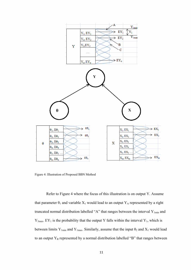
Figure 4: Illustration of Proposed BBN Method

Refer to Figure 4 where the focus of this illustration is on output Y. Assume

that parameter θ1 and variable X1 would lead to an output YA represented by a right

truncated normal distribution labelled “A” that ranges between the interval Y1min and

Y3max. EY1 is the probability that the output Y falls within the interval Y1, which is

between limits Y1min and Y1max. Similarly, assume that the input θ2 and X1 would lead

to an output YB represented by a normal distribution labelled “B” that ranges between

θ X

Y

 

12  

the interval Y1min and Y3max. EY2 is the probability that the output Y falls within

interval Y2 which ranges between Y2min and Y2max.

The truncated normal distribution “A” can be represented within the intervals

Y1, Y2 and Y3. The probability of the output YA falling within the three intervals are

shown below. The summation of Pr (YA1), Pr (YA2) and Pr (YA3) must add up to one.

Pr (YA1) = Pr (Y1min < YA < Y1max)

Pr (YA2) = Pr (Y2min < YA < Y2max)

Pr (YA3) = Pr (Y3min < YA < Y3max)

In the same vein, the normal distribution “B” can be represented within the

intervals Y1, Y2 and Y3. The probability of the output YB falling within the three

intervals are shown below. The summation of Pr (YB1), Pr (YB2) and Pr (YB3) must

add up to one.

Pr (YB1) = Pr (Y1min < YB < Y1max)

Pr (YB2) = Pr (Y2min < YB < Y2max)

Pr (YB3) = Pr (Y3min < YB < Y3max)

EY1 can then be calculated based on the sum of all the distribution overlaps

between Y1min and Y1max. The generalized equation can be represented by:

EY Pr Y  | θ   θ   θ X X X  

              Pr Y  | θ   θ   θ X X X  

Similarly, EY2 is calculated based on the sum of all the distribution overlaps

between Y2min and Y2max. The generalized equation can be represented by:

 

13  

EY Pr Y  | θ   θ   θ X X X  

              Pr Y  | θ   θ   θ X X X  

Pr Y  | θ   θ   θ X X X

Note that the summation of EY1, EY2 … EYo must add up to one. Table 1

shows a generalized representation of the CPT of output Y:

 

Table 1: Generalized representation of CPT of output Y

 

 

                                           

The methodologies of the proposed approaches in modeling complex physical

system that was described in this chapter would be further discussed in the next

chapter. 

 

 

14  

Chapter 3: Fuzzy Logic Modeling

 

Fuzzy systems represent a unique approach to represent uncertainties that

usually arise from complex systems. As quoted by Lotfi A. Zadeh, “As the complexity

of a system increases, it becomes more difficult and eventually impossible to make a

precise statement about its behavior, eventually arriving at a point of complexity

where the fuzzy logic method born in humans is the only way to get at the

problem.” [8].

A fuzzy system is deterministic and time invariant where the input and output

parameters are encoded in fuzzy representations and the interrelationships between

the fuzziness take the form of well defined if/then rules. The fuzzy system then

converts these rules to their mathematical equivalents, which would simplify the

interaction between the human and computer. This in turn offers a more realistic and

accurate representation of system behavior in the real world.

Fuzzy logic deals with reasoning that hinges on approximation rather than

precision. This presents a stark contrast to crisp logic where binary sets have binary

logic and the logic variables have a membership value of either 0 or 1.

The Fuzzy Logic Toolbox [2] can be used to create a fuzzy logic system. This

toolbox is a collection of functions built on the MATLAB numeric computing

environment which enables one to create and edit fuzzy inference system within the

MATLAB interface. The implementation of this function with an existing application

will be discussed in Chapter 5 of this paper.

 

15  

Several definitions relating to the fuzzy logic modeling are given as follows:

(1) Membership Function: A characteristic function pertaining to a simple and

versatile mathematical tool for indicating flexible membership to a set. [9]

(2) Fuzzy Set: Any set that allows its members to have different grades of

membership function in the interval [0, 1]. [10]

(3) Universe of Discourse: A range of all possible values of an input into a fuzzy

control system.                          [10] 

Properties of Fuzzy Sets [9]:

Double Negation Law

Idempotency

Commutativity

Associative Property  

 

Distributive Property  

 

Absorption

De Morgen’s Laws =

    =    

 

16  

3.1 Fuzzification

 

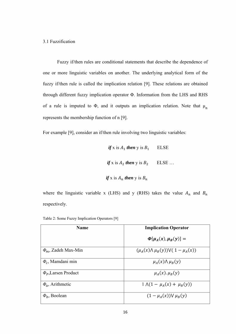
Fuzzy if/then rules are conditional statements that describe the dependence of

one or more linguistic variables on another. The underlying analytical form of the

fuzzy if/then rule is called the implication relation [9]. These relations are obtained

through different fuzzy implication operator Φ. Information from the LHS and RHS

of a rule is imputed to Φ, and it outputs an implication relation. Note that μ

represents the membership function of n [9].

For example [9], consider an if/then rule involving two linguistic variables:

if x is then y is  ELSE

if x is then y is ELSE …

if x is then y is

where the linguistic variable x (LHS) and y (RHS) takes the value and

respectively.

Table 2: Some Fuzzy Implication Operators [9]

Name Implication Operator

,

, Zadeh Max-Min  1

, Mamdani min  

,Larsen Product .

, Arithmetic 1 1  

, Boolean 1  

 

17  

, Bounded Product 0    1

 

 

Table 3: Interpretation of ELSE under some Implication [9]

Implication Interpretation of ELSE

, Zadeh Max-Min AND ( )

, Mamdani min OR ( )

,Larsen Product OR ( )

, Arithmetic AND ( )

, Boolean AND ( )

, Bounded Product OR ( )

 

 

3.2 Defuzzification Methods  

Defuzzification [9] is a process of selecting a crisp number u* representation

from the membership function output µ . This step takes place after the inputs to the

controller has been processed by the fuzzy algorithm. The most commonly used

defuzzification methods are COA, COS, and MOM.

3.2.1 Center of Area Defuzzification The crisp value u* is taken to be the

geometrical center of the output fuzzy

value μ , where μ is the union of all

the contributions of rules whose DOF >

 

18  

0.

u  ∑ u μN u∑ μN u

Where is the universe of discourse and

N is the number of samples. It is a

commonly used defuzzification method,

and is also known as Centroid.

 

3.2.2 Center of Sums Defuzzification

Easy to implement, and has fast

inference cycle. COS takes into

account the overlapped areas of

multiple rules more than once.

COS takes the sum of the outputs

from each contributing rule and not

just the union.

 ∑ ∑ ′

∑ ∑ ′

Where ′ is the membership

function resulting from firing the kth

rule.

 

19  

3.2.3 Mean of Maxima Defuzzification

Takes the crisp value with the highest

degree of membership in (u).

   

is the mth element in the universe

of discourse where membership

function is at the maximum value,

and M is the total number of such

elements.

Faster than COA and allows controller

to reach values near the edges of the

universe of discourse.

 

 

20  

Chapter 4: Bayesian Belief Network  

Bayesian belief network is a powerful tool for modeling causes and effects in

systems and is sometimes described as a marriage between probability theory and

graphical theory [11]. BBN represents compact networks of probabilities that capture

the probabilistic relationships between variables, as well as historical information on

their relationships. From another perspective, BBN is a combination of Bayesian

probability theory and the notion of conditional independence [12]. BBN is also

known as belief network, causal graph, causal network, probabilistic network, or

influence diagram.

Bayesian belief network allows for clear graphical representation of causes

and effect; and are effective for modeling scenarios where some prior information is

already known but input data is uncertain, vague, conflicting or partially unavailable.

BBNs are defined as: 1) DAG that represent probabilistic dependency models; 2)

DAG with nodes representing random stochastic/uncertain variables [7]; and 3) the

arcs that represent the Bayesian probabilistic relationships/influences between these

variables. BBN uses Bayes theorem to express conditional probability between each

event/alternative. It is also known as a network of nodes of influences based on

reasoning.

Some advantages [11] of BBN are listed as follows:

• Exact historical data or evidence is not necessary to produce convincing

results.

• The ability to provide effective output despite of uncertainties in the input

information.

 

21  

• Able to display variables in a model as nodes in a network, and causes and

effects as links between the nodes.

• Able to diagnose current situation based on past data.

An example of a BBN extracted from Adnan Darwiche’s paper [7] is shown below:

Figure 5: Bayesian Network over five propositional variables [7]

Figure 5 shows a BN with five nodes, Z = {A, B, C, D, E}. The five tables are

known as CPT ΘB|A  where it denotes the CPT for variable B, and its parent A.  θ | is

used to denote the value assigned by the CPT ΘB|A  to the conditional probability Pr

 

22  

(b|a). Note that the sum of  θ | must add up to one. In addition, conditional

probabilities represent the likelihoods based on prior or historical information.

Based on the above BN, the probability of winter being true given the

conditions that sprinkler is on; there is no rain; grass is wet; and road is not slippery is

as follows:

Pr  , , , , ) =   θ  θ |   θ |   θ | ,   θ |

= (0.6) * (0.2) * (0.2) * (0.9) * (1) = 0.0216

Similarly, the probability that winter is false, given the conditions that

sprinkler is off, there is no rain, grass is not wet and road is not slippery is as follows:

Pr  , , , , ) =   θ  θ |   θ |   θ | ,   θ |

= (0.4) * (0.25) * (0.9) * (1) * (1) = 0.09

Further explanations on the terminology of the BBN can be found in Appendix B.

 

23  

Chapter 5: Applications of Proposed Bayesian Belief Network and Fuzzy Logic Models

 

A pump system application is used to illustrate the employment of the

proposed BBN method and FLM in dynamic systems. This application is adapted

from previous research done by Y.S. Hu [3], where it demonstrates the modeling

dynamic behavior of a pump to avoid cavitation from occurring at the suction head.

One important parameter for measuring pump cavitation at the inlet is the NPSHA,

which is the difference between the sum of the velocity and the pressure heads, and

the vapor pressure head. Studying the POF of this application is accomplished by

obtaining the optimal values of three input parameters  , GPM and Temperature as

shown in Figure 7, such that NPSHA will not reach negative, which would otherwise

cause the pump suction head to break. In this application, it should be noted that

represents the distance below the pump that extends to the free water surface of the

reservoir; ‘GPM’ is proportional to the speed of the pump; and ‘Temperature’ is the

temperature of the free water surface of the reservoir.

This application involves implementing the proposed BBN model and FLM

respectively to estimate the NPSHA results based on the three input parameters.

Results obtained from the two methodologies are then compared with a reference

NPSHA data obtained via the implementation of a mathematical model [3]. The

advantages and disadvantages of the BBN and FLM would be discussed in detail at

the end of this thesis.

To better understand how the DMLD works in Figure 7, refer to Appendix A

for the Notations of DMLD based on time dependent fuzzy logic.

 

24  

Figure 6: A Pumping System [3]

 

Figure 7: DMLD for simulating NPSHA [3]

NPSHA1

 

25  

5.1 Mathematical Model  

Consider the system where 100  and the pipe is 4 inches in diameter.

For a given relative installation location of a pump-sink set, the NPSHA can be

expressed as:

NPSHA 35.18 Z  6.4 10 GPM  0.085 Temperature   ͦ F [3]

The pump GPM ranges between 0 and 480 and temperature falls in the range

of 0 to 200 ͦ F. Note that Z = 0 would give the worst case scenario for NPSHA at any

given GPM and Temperature data. Thus to simplify this application, Z is assumed to

be zero.

Figure 8: Numerical representation of NPSHA vs. GPM

 

NPSHA’s output calculation of six different temperature ranges was based on

the physical model. These data is used as the reference data for comparison between

the FLM and the proposed BBN Model. Figure 8 captures the plot of GPM vs.

 

26  

NPSHA when = 0. As the distance between pump and water surface increases,

NPSHA adjusts according to the increase in  .

5.2 Fuzzy Logic Model  

The first step of developing the FLM is to define the rules (Figure 9) based on

the input conditions mapped by the DMLD as shown in Figure 7. The fuzzy logic

illustration of the Pump System when = 0 is shown in Figure 10.

GPM

HI MH MD ML LW ZE

TEMP HI A B C D E F

LW G H I J K L

Figure 9: Rules based between Temperature and GPM

 

 

Figure 10: Fuzzy logic illustration of Pump System at = 0

G1 G2 G3 G4 G5 G6

T1 A B C D E F

T2 G H I J K L

NPSHA1 

Temp  GPM 

 

27  

Assumptions made in the application of this model are shown in Table 4.

Table 4: Temperature and GPM Category breakdown

Temperature Range Category Symbol

0 to 100 deg F Low TempLW

101 to 200 deg F High TempHI

GPM Range Category Symbol

-40 to 40 Zero ZE

0 to 120 Low LW

80 to 200 Mid Low ML

160 320 Mid MD

280 to 400 Mid High MH

360 to 480 High HI

MATLAB’s FLT function was used in this instance where the FIS structure is

a MATLAB object that contains all the fuzzy inference system information.

 

28  

Figure 11: FIS interface with 2 input and 1 output parameter

 

 

Figure 12: Membership function of Temperature

The input Temperature is made up of a Z-shaped and S-shaped membership

function.

 

29  

Figure 13: Membership function of GPM

The GPM inputs are made up of triangular-shaped membership functions, and

the Z/S shaped membership functions at the extreme ends.

Figure 14: Membership function of output NPSHA1

 

30  

The fuzzy output of NPSHA1 is represented by letters A to L. These fuzzy

modes are made up of triangular-shaped membership function as shown in Figure 14.

The implication operator that was used to work out the fuzzy algorithm is the

Mamdani Min, as discussed in Section 3.1

Figure 15: Rules conditions between input and output parameters

Note that the rules as shown in Figure 15 are defined based on the DMLD

(Figure 7). The fuzzy NPSHA1 output goes through a defuzzification process via

COA method, as discussed in Section 3.2.1 so as to obtain crisp values for the output.

 

31  

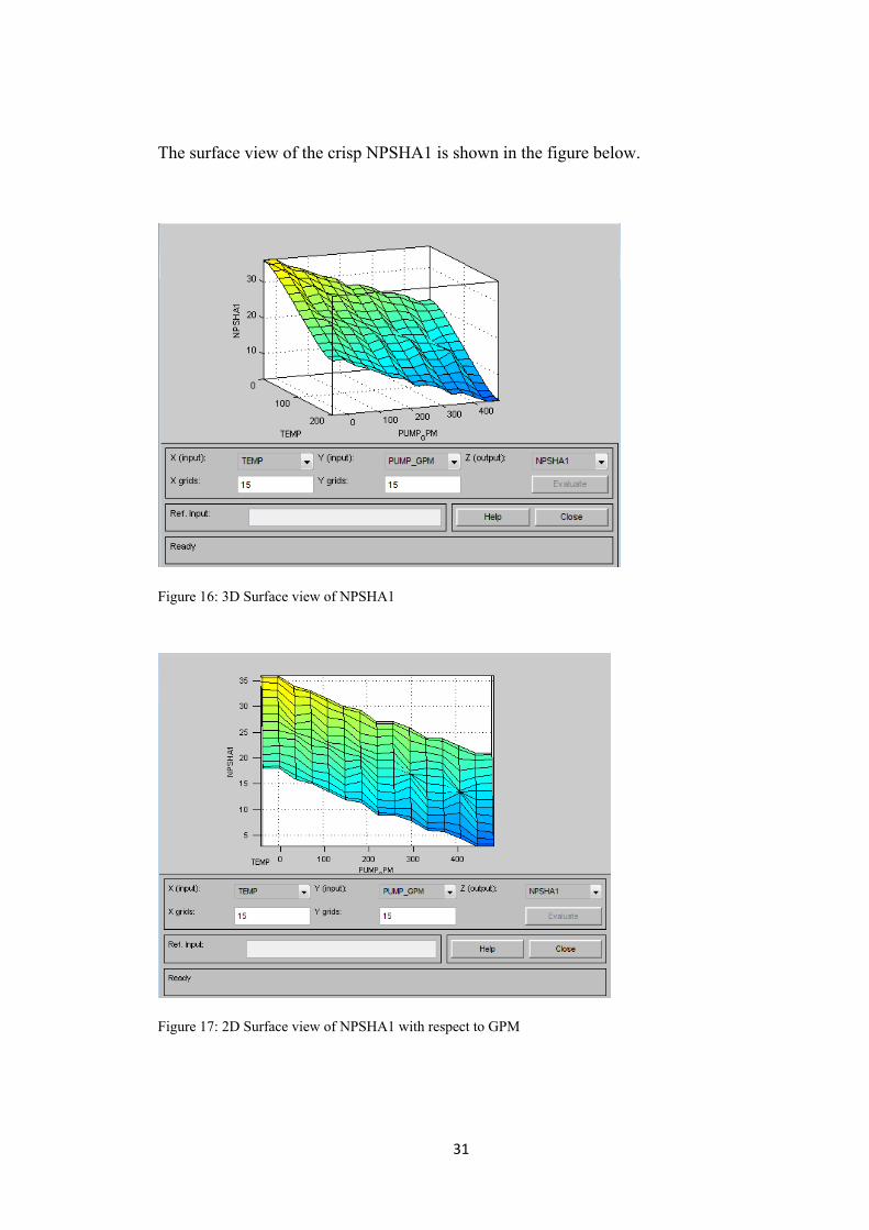
The surface view of the crisp NPSHA1 is shown in the figure below.

Figure 16: 3D Surface view of NPSHA1

Figure 17: 2D Surface view of NPSHA1 with respect to GPM

 

32  

Figure 18: Pump GPM vs. NPSHA1

 

Figure 18 shows the visualization of the NPSHA1 output with respect to

Temperature and GPM. From the surface view of NPSHA1, GPM vs. NPSHA ( =0)

is plotted and compared with the reference plot obtained via the mathematical model.

The trends of the graphs at all 6 temperature points are consistent with the reference

plot as shown in Figure 8. It is not possible to obtain precise output solution as FLM

is based on approximation given limited input and output data. In order to obtain a

smoother curve with higher resolution, the membership functions of the input/output

parameters needs to be broken down into more defined categories, and fuzzy rules

need to be defined with greater accuracy.

 

33  

The output of NPSHA can be estimated by incorporating with NPSHA1

using the FIS controller as shown in Figure 19. NPSHA output can be estimated by

using the same methodology to estimate the initial NPSHA1.

Figure 19: FIS of NPSHA with parameter

Figure 20: Membership function of

 

34  

The membership function of is grouped into either positive or negative

category. Similarly, the membership function of NPSHA1 at individual temperature is

grouped according to five categories: NE, SN, NT, SP and PT. For this application,

the area of focus would be on NPSHA1 when temperature is zero. The fuzzy

NPSHA1 output range is shown in Figure 21, when T=0 is between 21 and 36, and

the triangular membership function is distributed across the output range.

Figure 21: Membership function of NPSHA1 at Temp = 0

Figure 22: Membership function of NPSHA at Temp =0

 

35  

The fuzzy output of NPSHA is then represented by the triangular membership

function labeled M to V as shown in Figure 22

Figure 23: Surface view of NPSHA at T=0 with respect to NPSHA1 and Z0

Referring to the surface view of output in Figure 23, the trend reveals that

NPSHA increases proportionally with Z0 increase. This estimated result is reasonable

given that the result obtained from the mathematical model in Section 5.1 is similar,

where NPSHA also exhibits a proportional increase when Z0 increases.

The same steps were repeated to obtain the corresponding fuzzy outputs of

NPSHA at temperatures of 40 ͦ F, 80 ͦ F, 120 ͦ F, 160 ͦ F and 200 ͦ F respectively.

5.3 Proposed Bayesian Belief Network Model  

Similar to the fuzzy logic method, BBN methodology adopts a probabilistic

approach to estimate the output NPSHA. Consider the case where inputs of the system

follow a normal distribution. To solve NPSHA1, is assumed to be zero. Using

Monte Carlo simulation for a sample size of 5000, both the inputs Temperature

 

36  

(0degF to 200degF) and GPM (0 to 480) were randomly sampled to form a normal

distribution as shown in Figure 24.

Mean = 100, Standard Deviation = 80  

  Mean = 250, Standard Deviation = 30

Figure 24: Normal distribution for input Temperature and GPM

 

 

 Figure 25: PDF and CDF of NPSHA1output

Assumptions made were based on expert opinions that suggested a NPSHA1

output range of 6.5 to 35. Monte Carlo simulation was used to generate this output

assuming a normal distribution of mean 23 and standard deviation of 3.6. (Refer to

Figure 25).

 

37  

Note that if the mathematical model were available, the two input distributions

can be fitted into the equation to generate a NPSHA1 output which follows a normal

distribution. The equation of NPSHA1 is the same as the NPSHA equation [3] in

section 5.1, except that the parameter is removed since it is considered to be zero.

In reality, it is more often than not that the mathematical Model of a system is

usually not available, and this is especially true for new systems which still lack

established model testing. BBN is therefore a useful tool to estimate the output of the

system.

Figure 26: Histogram of NPSHA1 to estimate the probability of A to L

The normal distribution of NPSHA1 is divided equally into 12 columns as

shown in the histogram of Figure 26. The histogram is aligned to the state A to L of

the DMLD as shown in Figure 7 assuming no overlap and uncertainty between the

states. The probabilities of A to L estimated based on the CDF of NPSHA1 (Figure

25) are tabulated in Table 5:

 

38  

Table 5: Probability data and value of A to L based on the CDF of NPSHA1

Gmax 23.06 2.28E-01

Hmax 25.414 2.53E-01

Imax 27.767 1.86E-01

Jmax 30.12 9.06E-02

Kmax 32.473 2.91E-02

Lmax 34.826 6.19E-03

NPSHA1 min 6.59

The probabilities of GPM and Temperature inputs as shown in Table 6 are

estimated based on the CDF of inputs GPM and Temperature.

Table 6: Probability data of GPM and Temperature inputs

Input Symbol Range Probability

GPM HIGH GHI 391-480 2.79E-02

GPM MID HIGH GMH 301-390 1.95E-01

GPM MID GMD 181-300 5.51E-01

GPM MID LOW GML 91-180 1.96E-01

GPM LOW GLW 1 – 90 2.81E-02

GPM ZERO GZE 0 1.29E-03

TEMP LOW TLW 0 – 100 4.82E-01

TEMP HIGH THI 100 - 200 5.18E-01

In the real world, uncertainties are inevitable, and it is not realistic to represent

the output of GPM and Temperature based on the NPSHA’s DMLD structure.

Instead, it is more feasible to spread the outputs of GPM and Temperature over a

range of values represented by a distribution.

NPSHA1 Probability

Amax 8.9431 2.12E-05

Bmax 11.296 2.70E-04

Cmax 13.649 2.38E-03

Dmax 16.002 1.39E-02

Emax 18.355 5.34E-02

Fmax 20.708 1.36E-01

 

39  

To prove that overlaps do exist over the A to L states of NPSHA1 output, the

two extreme ends of each GPM and Temperature category are substituted into the

physical equation of NPSHA1. The minimum/maximum GPM and Temperature

values are then tabulated in Table 7:

Table 7: Representation of GPM and Temperature variables

Symbol  Temp  TEMP 

THI2  HI_max  200

THI1  HI_min  101

TLW2  LW_max 100

TLW1  LW_min  0

The minimum/maximum values of A to L tabulated in Table 8 are computed

by subsituting minimum/maximum GPM and Temperature into the mathematical

model.

For example, based on the DMLD structure:

A1 35.18  6.4 10 GHI1  0.085 THI2

A1 35.18  6.4 10 480  0.085 200  3.4344

Symbol  GPM  Value 

GHI1  HI_max  480

GHI2  HI_min  391

GMH1  MH_max  390

GMH2  MH_min  301

GMD1  MD_max  300

GMD2  MD_min  181

GML1  ML_max  180

GML2  ML_min  91

GLW1  LW_max  90

GLW2  LW_min  1

GZE  ZE  0

 

40  

A2 35.18  6.4 10 GHI2  0.085 THI1

A2 35.18  6.4 10 391  0.085 101  16.8106

Symbol  NPSHA1  Value 

A1  A_min  3.4344

A2  A_max  16.81062

B1  B_min  8.4456

B2  B_max  20.79654

C1  C_min  12.42

C2  C_max  24.4983

D1  D_min  16.1064

D2  D_max  26.06502

E1  E_min  17.6616

E2  E_max  26.59494

F1  F_min  18.18

F2  F_max  26.595

Symbol NPSHA1 Value 

G1  G_min  11.9344 

G2  G_max  25.39562 

H1  H_min  16.9456 

H2  H_max  29.38154 

I1  I_min  20.92 

I2  I_max  33.0833 

J1  J_min  24.6064 

J2  J_max  34.65002 

K1  K_min  26.1616 

K2  K_max  35.17994 

L1  L_min  26.68 

L2  L_max  35.18 

From Table 8, note that the overlaps between A and L imply that uncertainties

do exist between the A to L states.

The DMLD of the pump system can be illustrated by a BBN as shown in

Figure 27. For this particular example, the area of focus would be on the comparison

of NPSHA1 (highlighted in red). The software used to develop the BBN is IRIS [13].

Table 8: Numerical values of A to L

 

41  

Figure 27: BBN interpretation of the pump system

In the perfect world, NPSHA1 can be represented based on the following

Bayesian model:

Pr 1 | 

Pr   

Pr 1 |  1 2

Pr  …

Pr 1 |  1 2

Pr 

Pr 1 |   Pr     

 

42  

This computation assumes no uncertainty between A and L. The probability

data of GPM and Temperature as shown in Table 6 would be entered into the GPM

and Temp node respectively. The conditional probability of A to L entered into the

NPSHA1 node is shown in Figure 28. Interpretations based on these conditions are

incorrect as there are overlaps in the NPSHA1 output data.

Figure 28: Conditional Probability table assuming no uncertainty between A to L

 

On the other hand, consider the case where the outputs of GPM and

Temperature are spread over a range of NPSHA1 distribution. The 12 output

combinations of GPM and Temperature are listed as follows:

Set1 represents the NPSHA1 output when GPM is HI and Temp is HI

Set2 represents the NPSHA1 output when GPM is MH and Temp is HI

Set3 represents the NPSHA1 output when GPM is MD and Temp is HI

Set4 represents the NPSHA1 output when GPM is ML and Temp is HI

Set5 represents the NPSHA1 output when GPM is LW and Temp is HI

Set6 represents the NPSHA1 output when GPM is ZE and Temp is HI

Set7 represents the NPSHA1 output when GPM is HI and Temp is LW

Set8 represents the NPSHA1 output when GPM is MH and Temp is LW

 

43  

Set9 represents the NPSHA1 output when GPM is MD and Temp is LW

Set10 represents the NPSHA1 output when GPM is ML and Temp is LW

Set11 represents the NPSHA1 output when GPM is LW and Temp is LW

Set12 represents the NPSHA1 output when GPM is ZE and Temp is LW

Assume that all 12 sets follow a normal distribution with the corresponding

estimated means and standard deviations that are listed in Table 9. The distributions

between these sets have overlaps where more specifically, set 1 follows a left sided

truncated normal distribution, and set 12 follows a right sided truncated normal

distribution. The overlapped areas for each set would be summed up according to the

NPSHA1 groups.

Table 9: Mean and Standard Deviation of 12 sets

Sets  Mean  SD 

1  10  2

2  14  2

3  18  2

4  21  1.5

5  22  1.2

6  23  1.2

Sets  Mean  SD 

7 19 2 

8 23 2 

9 27 2 

10 29 2 

11 30 2 

12 31 1.5 

MATLAB was used to compute the weights for the states A to L for each set.

To illustrate this method, the derivation of Sets 1 and 2 would be explained in greater

depth as follows.

Truncated normal distribution

The PDF of the truncated normal distribution is represented by the equation:

|  , , ,1

 

 

44  

Where X ~ N (μ,σ2), X ϵ (a,b), -∞ ≤ a < b ≤ ∞. If b → ∞, then = 1; and if a → -∞, then = 0.

The CDF of the truncated normal distribution is represented by the equation:

|  , , , 

 

Similarly, if b → ∞, then = 1; and if a → -∞, then = 0.

The range of set 1 is first estimated, which is approximately between 3 and 17;

and represented by a normal distribution. Since set 1 is left truncated at a = 6.59 and b

→ ∞, the PDF of set 1 is given by:

|  , , 6.59,∞1

1   6.59

Similarly, the CDF of this set is given by:

|  , , 6.59,∞  6.59

1   6.59

where the respective μ and σ values can be obtained from Table 9.

The PDF plot of set 1 is shown in Figure 29. The blue plot represents the

normal distribution while the red line represents the truncated normal distribution.

 

45  

Figure 29: PDF of Set 1 which represents the GPM_HI and Temp_HI

Figure 30: CDF of Set 1 which represents the GPM_HI and Temp_HI

 

6.59 

6.59 

 

46  

The CDF of set 1 is shown in Figure 30. The blue plot represents the normal

distribution while the red line represents the truncated normal distribution. In addition,

set 1 assumes the range of A to E (referring to Table 5) which is represented by A1 to

A5 respectively. The probabilities of A1 to A5 are given as follows:

Pr (A1) = 2.63E-01

Pr (A2) = 4.66E-01

Pr (A3) = 2.35E-01

Pr (A4) = 3.34E-02

Pr (A5) = 1.30E-03

Working out the probabilities of set 2, the PDF and CDF graphs are plotted in

Figures 31 and 32 respectively:

Figure 31: PDF of set 2 which represents the GPM_MH and Temp_HI

 

47  

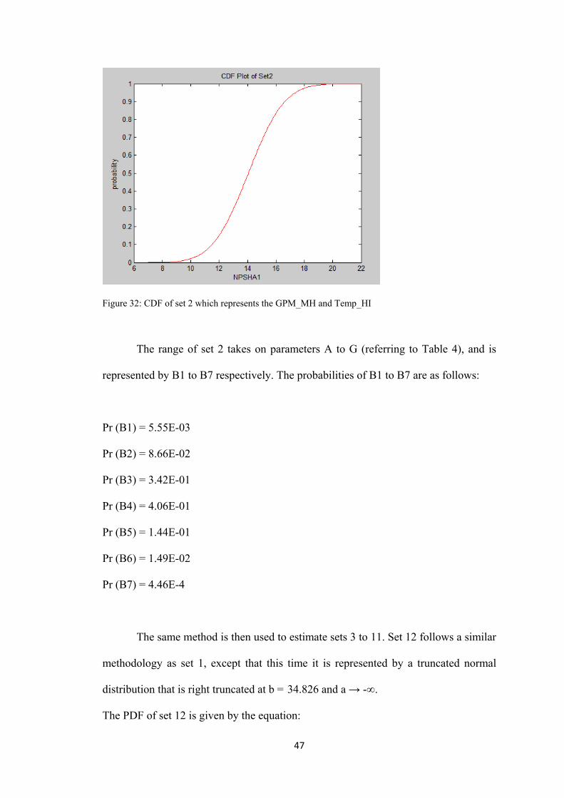
Figure 32: CDF of set 2 which represents the GPM_MH and Temp_HI

 

The range of set 2 takes on parameters A to G (referring to Table 4), and is

represented by B1 to B7 respectively. The probabilities of B1 to B7 are as follows:

Pr (B1) = 5.55E-03

Pr (B2) = 8.66E-02

Pr (B3) = 3.42E-01

Pr (B4) = 4.06E-01

Pr (B5) = 1.44E-01

Pr (B6) = 1.49E-02

Pr (B7) = 4.46E-4

The same method is then used to estimate sets 3 to 11. Set 12 follows a similar

methodology as set 1, except that this time it is represented by a truncated normal

distribution that is right truncated at b = 34.826 and a → -∞.

The PDF of set 12 is given by the equation:

 

48  

|  , , ∞, 34.381

34.38

Similarly, the CDF of set 12 is given by:

|  , , ∞, 34.38 34.38

where the respective μ and σ values can be obtained from Table 8.

Figure 33: PDF of set 1 which represents the GPM_ZE and Temp_LW

 

Figure 33 illustrates the graphical representation of PDF of set 12. The blue

plot represents the normal distribution while the red line represents the truncated

normal distribution. Note that there is only a slight truncation to the right that results

in a small change in the PDF.

 

49  

Figure 34: CDF of set 12 which represents the GPM_ZE and Temp_LW

 

The CDF of set 12 is represented by the graph in Figure 34. The blue plot

represents the normal distribution while the red line represents the truncated normal

distribution. After computing the probability distributions for all 12 sets, the

probability of the weights of each set can be estimated. The results are entered into the

CPT as shown in Figure 35.

Figure 35: Conditional probabilities of A to L

0 0 0 0 0 0 0 0

 

50  

S1 = Pr (GHI) ∩ Pr (THI)

S2 = Pr (GMH) ∩ Pr (THI)

S3 = Pr (GMD) ∩ Pr (THI)

S4 = Pr (GML) ∩ Pr (THI)

S5 = Pr (GLW) ∩ Pr (THI)

S6 = Pr (GZE) ∩ Pr (TLW)

S7 = Pr (GHI) ∩ Pr (TLW)

S8 = Pr (GMH) ∩ Pr (TLW)

S9 = Pr (GMD) ∩ Pr (TLW)

S10 = Pr (GML) ∩ Pr (TLW)

S11 = Pr (GLW) ∩ Pr (TLW)

S12 = Pr (GZE) ∩ Pr (TLW)

Note that the probability values of GPM and Temp can be found in Table 6.

The probabilities of A to L can be estimated by adding up the overlaps. For example,

Pr (A) = A1 * S1 + B1 * S2

= 2.63E-01 * 1.44E-02 + 5.55E-03 * 1.01E-01 = 4.37 E -3

Pr (B) = A2 * S1 + B2 * S2 + C2 * S3 + G2 * S7

= 4.66E-01 * 1.44E-02 + 8.66E-02 * 1.01E-01 + 3.44E-04 * 2.85E-01 + 4.43E-5 *

1.34E-02 = 1.56E-02

Applying the same calculations to the rest of the parameters, Table 10 lists the

estimated probabilities of A to L using the BBN structure shown in Figure 27.

Symbol Value S1 1.44E-02S2 1.01E-01S3 2.85E-01S4 1.01E-01S5 1.45E-02S6 6.71E-04S7 1.34E-02S8 9.39E-02S9 2.65E-01S10 9.43E-02S11 1.35E-02S12 6.24E-04

 

51  

Table 10: Probability of A to L

Symbols  Probability  Cumulative 

A  4.37E‐03  4.37E‐03

B  1.56E‐02  2.00E‐02

C  4.18E‐02  6.18E‐02

D  8.25E‐02  1.44E‐01

E  1.42E‐01  2.86E‐01

F  1.58E‐01  4.44E‐01

G  1.28E‐01  5.72E‐01

H  1.03E‐01  6.75E‐01

I  1.50E‐01  8.25E‐01

J  1.26E‐01  9.51E‐01

K  4.32E‐02  9.94E‐01

L  6.16E‐03  1.00E+00

The following chapter will compare and analyze the results obtained via the

two methodologies. The respective pros and cons of both BBN and FLM will also be

discussed.

 

52  

Chapter 6: Findings and Discussion  

This section discusses the probability data of NPSHA1 obtained from the

BBN model based on the assumption of whether uncertainty is incorporated into

constructing the BBN. The probability data and NPSHA1 data are tabulated in Table

10.

Comparisons will also be made on both BBN model and FLM with respect to

the reference model which for this case is the mathematical model. The criteria for

comparisons are as follows:

• Accuracy of results*

• Resolution of data*

• Flexibility in model adjustment

• Ease of building the model

• Ability to update the model

• Requirement for precise data

• Mathematical strength

• Areas of application

The strengths and weaknesses of the two methodologies are also discussed as

a follow up to the comparisons.

* Note that some of the comparisons are made in the context of the pump system

application.

 

53  

6.1 Discussion on Bayesian Belief Network Probability Data  

In the comparison of the probability data of NPSHA1, the assumption of

whether uncertainty is incorporated gives rise to the following two scenarios (Refer to

Table 11 for the comparisons of probability data of NPSHA1 based on the two

scenarios):

Scenario 1: Bayesian Belief Network with no uncertainty

Bayesian Belief Network methodology as discussed in section 5.3 was used to

estimate the NPSHA1 output, with no physical equation available. The input

parameters mapped to the NPSHA1 output range from A to L via a DMLD as shown

in Figure 7. IRIS [13] was used to model the BBN representation of the pump system.

The CPT as shown in Figure 28 was set up with the assumption of no uncertainty

between the outputs, given the GPM and Temperature input conditions.

Analyzing the “Probability with No Uncertainty” column in Table 11, the

probabilities of F and L are very low, suggesting that it is unlikely that the range of

NPSHA will fall in state F and state L. Further observation of the expected NPSHA1

output (refer to “Midpoint of NPSHA1a Interval” column) between D and G reveals

that the data are very close to each other which might raise some concern over the

credibility of the results obtained.

Since no uncertainty is assumed, the midpoint of NPSHA1 interval outputs for

each state from A to L are point estimates. This interpretation is not realistic as data

sources often lack precision, and consequently rarely produces point estimate results.

Given that there are uncertainties within the input parameters, one should also expect

uncertainties in the outputs of A to L. This issue is addressed in scenario 2.

 

54  

Scenario 2: Bayesian Belief Network considering uncertainty

Using BBN methodology can incorporate uncertainties for each of the output

A to L. This method assumes a normal distribution with estimated means and standard

deviations for A to L (refer to Table 9). The CPT, obtained in Figure 32 shows a

distribution for each GPM/Temp alternative. The summation of the overlaps between

the distributions of the input alternatives provides a good estimate of the probabilities

of A to L.

Analyzing the “Probability with Uncertainty” column in Table 11, the

probabilities of A to L are considerably evenly distributed, with the two ends of the

tail, A and L having smaller probabilities as compared to the rest. The range of

NPSHA1 between A to L are well spread out, indicating uncertainties between each

range. The results obtained from the assumption of uncertainty are more realistic and

would be used for further discussion in section 6.2.

 

55  

Table 11: Comparison of probability data of NPSHA1 based on 2 scenarios

Temp GPM

Probability

with No

Uncertainty Cumulative

Midpoint+ of

NPSHA1a

Interval

Probability

with

Uncertainty Cumulative

Midpoint+ of

NPSHA1b*

Interval

A 100-200 391-480 1.64E-02 1.64E-02 8.96 4.37E-03 4.37E-03 8.07

B 100-200 301-390 1.03E-01 1.19E-01 16.64 1.56E-02 2.00E-02 14.16

C 100-200 181-300 2.76E-01 3.95E-01 20.00 4.18E-02 6.18E-02 16.08

D 100-200 91-180 1.00E-01 4.95E-01 22.10 8.25E-02 1.44E-01 17.85

E 100-200 1 to 90 1.66E-02 5.11E-01 22.64 1.42E-01 2.86E-01 19.59

F 100-200 0 8.43E-04 5.12E-01 22.71 1.58E-01 4.44E-01 21.24

G 0-100 391-480 1.56E-02 5.28E-01 22.79 1.28E-01 5.72E-01 22.57

H 0-100 301-390 9.77E-02 6.26E-01 23.31 1.03E-01 6.75E-01 23.63

I 0-100 181-300 2.62E-01 8.88E-01 25.37 1.50E-01 8.25E-01 24.98

J 0-100 91-180 9.54E-02 9.83E-01 28.64 1.26E-01 9.51E-01 27.12

K 0-100 1 to 90 1.58E-02 9.99E-01 32.16 4.32E-02 9.94E-01 29.94

L 0-100 0 8.02E-04 1.00E+00 34.72 6.16E-03 9.98E-01 32.18

* NPSHA1b is normally distributed over the expected data. + Midpoint estimates used as the closest estimation for the mean of NPSHA1

 

56  

6.2 Comparison of NPSHA1 Data with Reference Data  

NPSHA1 output obtained via the BBN and FLM were compared to the

NPSHA1 output of the reference model over four different temperatures of 40, 80,

120 and 160 ͦ F. The results are tabulated in Tables 12 and 13.

6.2.1 Bayesian Belief Network Model Comparison and Discussion

Accuracy of results

The NPSHA1 estimated via BBN gives expected values over a range of

uncertainties. For example, given the assumption that GPM is zero and temperature is

low, NPSHA output is distributed across H to L. There is a 61% probability of being

in state K, which is estimated to be between the range of 26 and 36; and a 27%

probability of being in state J, which is estimated to be between 24 and 35 (As shown

in Figure 36). Note that the probability of state K dominates the other states.

Figure 36: Distribution of NPSHA given GPM and Temperature evidence

Pr (0<NPSHA1≤23 | GPM=0 ∩ 0<T≤100) =0

Pr (17<NPSHA1≤29 | GPM=0 ∩ 0<T≤100) =1.08E-4

Pr (20<NPSHA1≤33 | GPM=0 ∩ 0<T≤100) = 1.63E-2

Pr (24<NPSHA1≤35 | GPM=0 ∩ 0<T≤100) = 2.70E-1

Pr (26<NPSHA1≤36 | GPM=0 ∩ 0<T≤100) = 6.10E-1

Pr (27<NPSHA1≤36 | GPM=0 ∩ 0<T≤100) = 1.04E-1

Pr (0<T≤100) =1

Pr (GPM=0) =1

 

57  

Referring to Table 12 (highlighted in red), when GPM=0 and Temperature

=40 ͦ F, the midpoint of NPSHA1 output interval via BBN is 32.18, and has an

uncertainty range of 26 to 36. Compare this result with the reference NPSHA of

31.78. One would notice that there is no uncertainty in the GPM input when GPM

equals to zero while on the other hand, uncertainty exists in the input Temperature

parameter. Comparing the two results, there is a difference of approximately 1.26%,

which provides a reasonable estimate.

Consider another scenario where uncertainties exist for both inputs GPM and

Temperature. Using the same methodology, this time given that GPM is mid low and

temperature is high, NPSHA1 output is distributed across D to I. There is a 38%

probability of being in state F, which is estimated to be between the range of 18 and

27; and a 49% probability of being in state G, which is estimated to be between 12

and 27. Note that the probabilities of NPSHA1 falling in state F and G are relatively

higher as compared to the previous scenario.

Referring to Table 12 (highlighted in red), when GPM = 120 and T = 160 ͦ F,

the midpoint of NPSHA1 output interval via BBN is approximately 17.85, and has an

uncertainty range of 12 to 27. Compare this result with the reference NPSHA of

20.6584. Notice that the uncertainty range is larger, and the difference between the

expected NPSHA1 and the reference NPSHA1 is approximately 13.59%.

Total absolute error of the NPSHA1 data at Temperature = 40deg ͦF is

calculated to be 38.17, which was derived by aggregating all absolute error terms

within the temperature range as listed in Table 12. The total percentage error is

therefore given by S      S      

  100 ..

100 8.87%. Using the same

 

58  

computations for all error terms at Temperature = 160deg ͦF, the total percentage error

is found to be:   ..

100 10.89%.

The relatively low percentage errors at the two temperature points suggest

that the results obtained via BBN on the two scenarios do provide a satisfactory

estimate of NPSHA1, although the extent of the errors are still dependent on the

degree of uncertainty of the input variables. In this particular application, the data

obtained from the reference model all falls within the uncertainty range specified by

the BBN model for every scenario. The important question is: what is the range that

would be considered acceptable? In order to have more precise results, the input

parameters need to be better defined such that uncertainties can be reduced.

 

59  

Table 12: Comparison of NPSHA1data between BBN model and Reference model at T = 40, 80, 120 and 160 ͦ F

GPM T = 40 T = 80 T = 120 T = 160

REF BBN Error REF BBN Error REF BBN Error REF BBN Error

0 31.78 32.18 0.40 28.38 32.18 3.80 24.98 21.24 3.74 21.58 21.24 0.34

20 31.75 29.94 1.81 28.35 29.94 1.59 24.95 19.59 5.36 21.55 19.59 1.96

40 31.68 29.94 1.74 28.28 29.94 1.66 24.88 19.59 5.29 21.48 19.59 1.89

80 31.37 29.94 1.43 27.97 29.94 1.97 24.57 19.59 4.98 21.17 19.59 1.58

120 30.86 27.12 3.74 27.46 27.12 0.34 24.06 17.85 6.21 20.66 17.85 2.81

160 30.14 27.12 3.02 26.74 27.12 0.38 23.34 17.85 5.49 19.94 17.85 2.09

200 29.22 24.98 4.24 25.82 24.98 0.84 22.42 16.08 6.34 19.02 16.08 2.94

220 28.68 24.98 3.70 25.28 24.98 0.30 21.88 16.08 5.80 18.48 16.08 2.40

240 28.09 24.98 3.11 24.69 24.98 0.29 21.29 16.08 5.21 17.89 16.08 1.81

280 26.76 24.98 1.78 23.36 24.98 1.62 19.96 16.08 3.88 16.56 16.08 0.48

320 25.23 23.63 1.60 21.83 23.63 1.80 18.43 14.16 4.27 15.03 14.16 0.87

340 24.38 23.63 0.75 20.98 23.63 2.65 17.58 14.16 3.42 14.18 14.16 0.02

380 22.54 23.63 1.09 19.14 23.63 4.49 15.74 8.07 7.67 12.34 8.07 4.27

400 21.54 22.57 1.03 18.14 22.57 4.43 14.74 8.07 6.67 11.34 8.07 3.27

440 19.39 22.57 3.18 15.99 22.57 6.58 12.59 8.07 4.52 9.19 8.07 1.12

480 17.03 22.57 5.54 13.63 22.57 8.94 10.23 8.07 2.16 6.83 8.07 1.24

 

60  

Resolution of data

In this pump system example, the Temperature input parameter only assumes

dichotomous categories, namely: low (0-100 ͦ F) and high (101-200 ͦ F). Referring to

Table 12, the expected NPSHA1 outputs estimated via BBN are the same for

Temperature input 0 to 100 ͦ F; and 101 to 200 ͦ F respectively.

Similarly, GPM input is divided into 6 categories such that NPSHA1 output is

the same for every GPM input that falls within each category. Referring to Table 12,

GPM = 20, 40 and 80 all falls within GML category where this results in the same

expected NPSHA1 output of 31.469 with an uncertainty range between 20 to 32.

Therefore, such categorical classifications of parameters would reduce the sensitivity

of output results, and may fail to distinguish output values that correspond to the

different values of the same input category. Plotting GPM with respect to NPSHA1

would result in a discrete graph that represents a loss of resolution, instead of a

smooth curve as shown in Figure 8.

In order to improve the resolution, more conditions would need to be defined

in the input parameter nodes. This can be achieved by obtaining more information on

the input parameters As the CPT increases in size and complexity, more time would

be required to build the BBN model. In short, there is a corresponding increase in the

resolution of the output data with larger number of conditions defined for each input

node.

Flexibility in model adjustment

Representing the pump system as a BBN is a more flexible approach to solve

system problems. Consider a case where the NPSHA output is known and estimations

 

61  

are necessary for the input parameters. In this instance, expert opinion estimates that

the NPSHA output is approximately between 13 and 17, which falls within state D.

Setting the evidence of NPSHA node of the BBN to D, the input parameters can be

estimated based on the graphical representation of BBN as shown in Figure 37.

Figure 37: BBN of pump system given evidence that NPSHA1 is D

 

In order to achieve NPSHA1 output that falls within state D, there is a 51%

probability that GPM is in the mid high range and 47% probability of being in the mid

range. There is a 98.8% probability that temperature would fall in the high region.

Ease of building the model

Although building the structure of a BBN model is not difficult, the process of

understanding, identifying and estimating the probability data for each condition of

Pr (100< T≤200 | 13<NPSHA1<17) = 9.88E-01

Pr (0< T≤100 | 13<NPSHA1<17) = 1.16E-02

Pr (390< GPM≤480 | 13<NPSHA1<17) = 1.80E-02

Pr (300< GPM≤390 | 13<NPSHA1<17) = 5.09E-01

Pr (180< GPM≤300 | 13<NPSHA1<17) = 4.72E-01

Pr (90< GPM≤180 | 13<NPSHA1<17) = 6.33E-04

Pr (0< GPM≤90 | 13<NPSHA1<17) = 8.25E-08

Pr (GPM=0 | 13<NPSHA1<17) = 1.89E-11

Pr (13<NPSHA1<17) = 1 

 

62  

every node makes the modeling challenging and tedious. The model becomes

complicated when many uncertainties are being considered in the input parameters,

and overlapping data are expected within the output parameters.

Currently, there is no established method to incorporate BBN into a system

with cyclic network. This proves to be a major problem as many complex real life

systems consist of cyclic networks. To counter this limitation, Tang, Liu and Qian

[14] proposed using DBN model to solve complex real life system with feedback

loops.

To elaborate further, DBN is based on temporal time series data. Consider a

simple example [14] with a feedback loop A→B→C→A, where node C at time t has

an influence on node A at time t+1 (Refer to Figure 38).

Figure 38: Dynamic Bayesian Network with feedback loop [11]

Dynamic Bayesian Network can construct a cyclic regulation by dividing the

states of a variable by time slices [15]. Node A at time t has an influence on itself at

t+1, i.e. as shown in the dotted lines in Figure 39. Node C in this case is

primary time dependent where  .

 

63  

One recommendation is to implement DBN on a primary feedback loop if it

satisfies the primary time dependency requirements, i.e. Node C and ignore all trivial

time dependencies, i.e. Node A.

Figure 39: Time expansion of the dynamic network in Figure 34 [11]

In another paper, Z. Mohaghegh, R. Kazemi, and A. Mosleh [16] proposed

using hybrid modeling to address dynamic complex system with feedback loops. They

use simulation based techniques such as ABM [17] and SD [18] to model complex

model with impossible analytical solutions.

System Dynamics technique represents dynamic deterministic relations in

hybrid modeling environment and provides dynamic integration among various

modules/subsystems. These subsystems which can be modeled via various techniques

such as BBN would have their own inputs and outputs to the SD module.

Consequently, the entire hybrid model would have the relevant capability to capture

feedback loops and delays. The SD software used in this paper [16] was STELLA.

 

64  

For example, the hybrid model allows the targeted subsystem that is modeled

via BBN to be imported and processed inside SD which has delays and feedback

loops. The estimated value calculated from SD would then be exported back into the

BBN environment. Such integrated processes would pose as a good alternative to

resolve the challenges that arise from integrating BBN into systems with feedback

loops. Figure 40 shows a demonstration on how BBN can be integrated into a system

with feedback loops.

Figure 40: Training module within a SD environment [16]

This thesis implements the use of BBN on a simple two inputs - one output

system, to demonstrate that it is possible to model a dynamic system probabilistically.

However, incorporating uncertainty into a complex system using BBN is highly

challenging as uncertainty has to be considered in every parameter and condition.

Building a BBN on multiple hierarchies of complex systems would require much

more computational effort and time. Therefore such applications are often subjected

to constraints posed by the limited resources in the industrial context.

 

65  

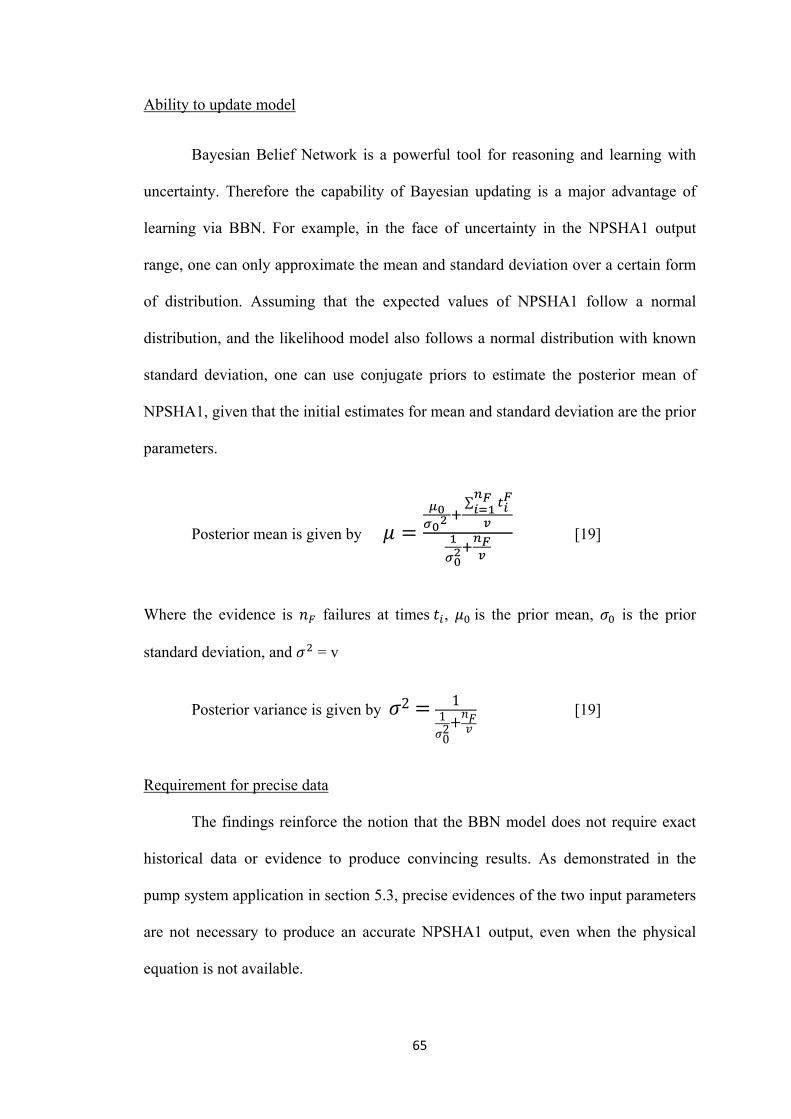
Ability to update model

Bayesian Belief Network is a powerful tool for reasoning and learning with

uncertainty. Therefore the capability of Bayesian updating is a major advantage of

learning via BBN. For example, in the face of uncertainty in the NPSHA1 output

range, one can only approximate the mean and standard deviation over a certain form

of distribution. Assuming that the expected values of NPSHA1 follow a normal

distribution, and the likelihood model also follows a normal distribution with known

standard deviation, one can use conjugate priors to estimate the posterior mean of

NPSHA1, given that the initial estimates for mean and standard deviation are the prior

parameters.

Posterior mean is given by   ∑

[19]

Where the evidence is failures at times  ,  is the prior mean, is the prior

standard deviation, and = v

Posterior variance is given by   2 11

02

[19]

Requirement for precise data

The findings reinforce the notion that the BBN model does not require exact

historical data or evidence to produce convincing results. As demonstrated in the

pump system application in section 5.3, precise evidences of the two input parameters

are not necessary to produce an accurate NPSHA1 output, even when the physical

equation is not available.

 

66  

However accuracy of the output will be limited to the certainty of the input

parameters. Therefore, highly uncertain inputs are often accompanied by more

ambiguous outputs. Further research can look into the determination of the level of

uncertainties within the data that is deemed as acceptable.

Mathematical strength

Bayesian Belief Network is modeled after Bayes’ theorem which is a proven

and established mathematical model. As a result, BBN methodology is also well

documented and widely accepted among scholars and practitioners.

 

Areas of application  

One rule of thumb in using BBN is that it is highly effective for modeling

applications where some information is already known and incoming data is uncertain

or partially unavailable. It is especially useful when historical or current information

is vague, incomplete, conflicting and uncertain [11].

However, there is a flip side to every coin as BBN is not adapted to work in

applications with time delays and feedback loops. Tang, Liu and Qian [14], and Z.

Mohaghegh, R. Kazemi, and A. Mosleh [16] have proposed DBN and Hybrid

modeling respectively to counter these problems. BBN is also useful in applications

where the exact mathematical model is difficult or impossible to be determined.

 

6.2.2 Fuzzy Logic Comparison and Discussion  

Accuracy of results

 

67  

Using the FLM methodology as discussed in section 5.2, the NPSHA1 fuzzy

data can be estimated via the plot as shown in Figure 18. From the results obtained

from Table 13, Figure 41 illustrates the comparison of NPSHA1 between reference

and FLM data at Temperature = 40 ͦ F.

 

Figure 41: Comparison of NPSHA at T=40 between Reference model and FLM

With reference to Figure 41, at Temperature = 40 ͦ F, the trend of fuzzy logic

line is consistent with the physical model line. It is not possible to obtain precise

results produced by the reference model due to the fuzziness or uncertainty defined

for the input and output parameters. The fuzzy output is more accurate towards the

two extreme ends of plot and less accurate in the middle. Referring to Table 13

(highlighted in red), at Temperature =40 ͦ F and GPM = 120, the NPSHA1 Fuzzy

output is 27.67 as compared to the reference NPSHA1 of 30.86, where the difference

is approximately 10.3%. Referring to Table 13(highlighted in red), at Temperature

Ref

 

68  

=160 ͦ F and GPM=120, the NPSHA1 Fuzzy output is 14.33 as compared to the

reference NPSHA1 of 20.66, which translates into approximately 30% difference.

The total absolute error for NPSHA1 data at Temperature = 40deg ͦ F is 35.63,

which is obtained by summing up all absolute error terms at this temperature found in

Table 13.. The total percentage error is therefore calculated as S      S      

 

100 ..

100 8.28%. Similarly for Temperature = 160deg ͦ F, the total

percentage error is .

Assuming a fixed input GPM, as the temperature increases, the variation

between the fuzzy NPSHA1 and reference NPSHA1 becomes larger. Such inaccuracy

is due to the fact that input temperature has only two membership functions, resulting

in fuzzier outputs.

In a nutshell, fuzzy logic is tolerant of imprecise data. Fuzzy reasoning builds

this understanding into the process rather than tacking it at the end [2].

 

69  

Table 13: Comparison of NPSHA1data between Fuzzy Logic model and Reference Model at T = 40, 80, 120 and 160 ͦ F

GPM T = 40 T = 80 T = 120 T = 160

REF FUZZY Error REF FUZZY Error REF FUZZY Error REF FUZZY Error

0 31.78 33.69 1.91 28.38 29.60 1.22 24.98 24.40 0.58 21.58 20.31 1.27

20 31.75 31.24 0.51 28.35 26.35 2.01 24.95 24.64 0.31 21.55 19.77 1.78

40 31.68 30.59 1.09 28.28 26.78 1.50 24.88 22.23 2.65 21.48 18.57 2.91

80 31.37 30.81 0.56 27.97 26.57 1.40 24.57 21.43 3.14 21.17 17.19 3.98

120 30.86 27.67 3.19 27.46 23.60 3.86 24.06 18.40 5.66 20.66 14.33 6.33

160 30.14 27.67 2.47 26.74 23.60 3.14 23.34 18.40 4.94 19.94 14.33 5.61

200 29.22 24.45 4.77 25.82 20.15 5.67 22.42 15.85 6.57 19.02 11.55 7.47

220 28.68 24.90 3.78 25.28 20.57 4.71 21.88 15.43 6.45 18.48 11.10 7.38

240 28.09 24.98 3.12 24.69 20.57 4.13 21.29 15.43 5.86 17.89 11.02 6.87

280 26.76 24.45 2.32 23.36 20.15 3.21 19.96 15.85 4.11 16.56 11.55 5.01

320 25.23 21.12 4.11 21.83 16.83 5.00 18.43 13.17 5.26 15.03 8.88 6.14

340 24.38 21.67 2.71 20.98 17.60 3.38 17.58 12.40 5.18 14.18 8.33 5.85

380 22.54 20.71 1.83 19.14 16.70 2.44 15.74 12.17 3.56 12.34 8.20 4.13

400 21.54 20.41 1.13 18.14 15.89 2.25 14.74 12.00 2.74 11.34 7.77 3.57

440 19.39 19.22 0.17 15.99 14.98 1.01 12.59 11.18 1.41 9.19 6.76 2.42

480 17.03 18.98 1.94 13.63 14.57 0.93 10.23 9.43 0.80 6.83 5.02 1.81

 

70  

Resolution of data

Fuzzy data has better resolution as compared to the BBN model. Referring to

Figure 41, note that there is a decreasing trend in the fuzzy plot which is noticeably

consistent with the reference plot. In order to improve the resolution, the membership

functions for the input and output parameters should be broken down further into finer

details. As such, more if/then rules between the inputs and outputs would need to be

defined.

Flexibility in model adjustment

Fuzzy Logic Modeling offers higher flexibility in its ability to adjust and

change the boundaries and membership functions of both input and output parameters

with little effort. However, application is limited in situations where the designers

only have information regarding the output parameters, and will need to estimate an

unknown input parameter.

Ease of building the model

The process of adapting FLM into a complex system is relatively easy and

straightforward. FIS greatly depends on a number of conditional “if-then” rules in

order to model the system output. Although these rules are easy to write, if the

designers do not understand the system well, they would not be able to provide

sufficient rules to accurately describe the system.

Fuzzy logic can be adapted onto multiple hierarchies of complex systems by

using SIMULINK [20], which is a dynamic system simulator for MATLAB. It

supports linear and non linear systems, and can be modeled in continuous time,

sampled discrete time, or a hybrid of both. Using the graphical user interface

 

71  

provided, one can build multiple hierarchies of FIS controllers in complex systems

using top down or bottom up approach; integrate them via logic gates and connectors;

and simulate the defuzzified data at the allocated output.

Ability to update model

Updating of model can be done manually by adjusting the boundaries of the

input and output parameters, or changing the shape of the membership functions.

There is no mathematical model that can be used to update FLM, and analysts are

required to manually update the models.

Requirement for precise data

Fuzzy logic addresses incomplete/uncertain input and output parameters

directly by defining them with fuzzy sets that can be expressed in linguistic terms.

When implementing FLM using the pump system, the only information available is

the approximate range of the two input and one output parameters. The rules are

formulated based on the mappings of the DMLD between the input and output

variables.

The model does not require historical data, but prior knowledge of the system

is necessary. If there is insufficient information, the fuzzy logic controller would not

be able to accurately model the system output [2].

For the pump system example, the prior knowledge about the system is based

on the DMLD, which is sufficient to generate the basic rules for the fuzzy controller

to process and generate a reasonable consistent output.

 

72  

When historical data is not available, FLM can be built on expert opinions.

This allows one to draw on the experience of experts in the relevant fields who are

already familiar with the associated systems [2].

Mathematical strength

The interrelationship between the fuzziness within a system is represented by

simple if/then rules, which allows simple representations of fuzzy descriptions [8].

The rules and conditions for the pump system are generated based on the

DMLD which maps the input variables to the output variable. These rules are easy to

understand as compared to analyzing the DMLD maps.

There is little complicated mathematics when describing the if/then rules. This

methodology is relatively new and not widely documented to-date [2]. As such, FLM

is still not widely implemented into controllers to solve system problems.

Areas of application

Fuzzy logic is able to model non linear functions of complex system such that

a fuzzy system can be created to match any set of input-output data. It is useful in

complex applications, system controls and analysis designs where the exact

mathematical model is hard or impossible to be determined [8].

Fuzzy logic is an effective modeling application for systems laden with

ambiguities and uncertainties during the decision-making process. In the pump system

example, the uncertainty of the input Temperature, input GPM, and output NPSHA1

are estimated and translated into the boundaries of their membership functions. The

range for each category of the two input parameters is tabulated in Table 4.

 

73  

6.2.3 Comparison between Bayesian Belief Network and Fuzzy Logic Model  

This section summarizes the respective discussions made on the Fuzzy Logic

and BBN models relative to the reference model and evaluates the two methodologies

against each other. The comparison is shown in Table 14.

Figure 42 shows a graphical representation of NPSHA1 output at Temperature

= 40 ͦ F for the BBN, FLM and the reference model. Note that the fuzzy model has

better resolution than the BBN model. As calculated earlier in section 6.2.1 and 6.2.2,

at Temperature = 40 ͦ F, the BBN model has an error percentage of 8.87% as

compared to Fuzzy Logic Model which has an error percentage of 8.28%. This shows

that FLM has slightly better accuracy than the BBN model at Temperature = 40 ͦ F.

 

Figure 42: NPSHA1 comparison based on the reference model, FLM and BBN at Temp = 40.

   

Ref 

 

74  

Figure 43 shows a graphical representation of NPSHA1 output at Temperature

= 160 ͦ F for the BBN, FLM and the reference model. Again, it can be observed that

the fuzzy model has better resolution than the BBN model. As calculated earlier in

sections 6.2.1 and 6.2.2, at Temperature = 160 ͦ F, the BBN model has an error

percentage of 10.89% as compared to FLM which has an error percentage of 27.14%.

The significantly smaller error percentage derived by the BBN demonstrates that at

Temperature = 160 ͦ F, this model produces more accurate NPSHA1 data than the

FLM.

 

Figure 43: NPSHA1 comparison based on the reference model, FLM and BBN at Temp = 160

 

  As a round up to our comparisons made between the BBN and FLM, Table 14

summarizes the respective strengths and weaknesses of each methodology based on

the comparison criteria as outlined in Chapter 6.

Ref

 

75  

Table 14: Table of Comparison between BBN and Fuzzy Logic Models

Comparison Criteria Bayesian Belief Network Fuzzy Logic Modeling

1. Accuracy of results*

*Note that this criterion is

compared in the context of the

pump system application and may

not be generalized. Different

applications would produce

different results.

• The expected value of the output is more

accurate when there is less uncertainty in the

input parameters.

• The output is distributed over a range of

uncertainties.

• The output from the reference model falls

within the uncertainty range, thus satisfying

the criteria.

• Smaller percentage change in error at high

temperature as compared to the FLM output,

suggesting that BBN yields better accuracy at

Temperature = 160 ͦ F.

• Output data are point estimates that

follow a consistent trend when

compared to a reference data.

• Slightly smaller percentage change in

error at Temperature = 0 ͦ F as compared

to the BBN output, which concluded

that FLM produces slightly more

accurate results than BBN at

Temperature = 0 ͦ F.

 

76  

2. Resolution of data*

*Note that this criterion is

compared in the context of the

pump system application and may

not be generalized. Different

applications would produce

different results.

• Relatively poor resolution that greatly

depends on the number of conditions being

defined in each input nodes.

• Unable to accurately estimate output data

when several inputs fall within a categorical

range as specified by the conditions. This

reduces sensitivity of the output results.

• Better resolution as compared to the

BBN model.

• Increases the number of membership

functions so as to reduce the fuzziness,

and as a result, improve the resolution.

3. Flexibility in model

adjustment

• Given that the evidence is known for certain

nodes, one would be able to estimate the

probability output of another node. This

would provide flexibility in estimating

required data.

• Less flexibility over estimating required

data given that some data are unknown.

• Designers must have a good knowledge

of the system in order to effectively use

FLM.

 

77  

4. Ease of building the model • BBNs are easy to build, but estimating and

assigning probabilities to every condition

within the node is tedious and time

consuming.

• Difficult to implement BBN in multiple

hierarchies of complex system.

• Hybrid modeling/SD could be used to

incorporate BBN into a system with time

delays, cyclic network and multiple

hierarchies of complex systems.

• Straightforward and easy to implement

Fuzzy Logic into a complex system, but

FIS greatly depends on a number of

conditional “if-then” rules in order to

model the system output.

• SIMULINK can be use to integrate

multiple FIS controller into a system

with time delays, cyclic network and

multiple hierarchies of complex

systems.

5. Ability to update

• The model has the ability to use Bayesian

• Updating of model can be done

 

78  

updating methodology to learn and train data.

This is a more formal methodology and has a

stronger mathematics basis for using it.

manually by adjusting the fuzzy sets of

the input and output parameters, or

changing the shape of the membership

functions.

• In case of new information, Fuzzy rules

need to be changed. Updating can only

be done by analyst.

6. Requirement for precise

data

• The model does not require exact historical

data or evidence to produce convincing

results.

• Accuracy of the output will be limited to the

certainty of the input parameters. Therefore,

highly uncertain inputs are often accompanied

by more ambiguous outputs.

• There is no need for precise data, but

designers need to understand how the

system operates in order to generate

sufficient if/then rules for the FIS

controller to produce an accurate

output.

 

79  

7. Mathematical strength

• Follows Bayes theorem which is an

established and proven model.

• Methodology has been used widely used in

many applications and is well documented.

• Fuzzy algorithm follows the if/then

rules, which uses basic mathematics.

• Methodology is relatively new, and is

not well accepted yet.

8. Areas of application • Effective for modeling applications where

some information is already known and

incoming data is uncertain or partially

unavailable.

• Useful in applications where the

mathematical model is hard or impossible to

be determined.

• Appropriate for diagnostic applications where

frequent updating of data is necessary.

• Effective for modeling applications

with ambiguities and uncertainties.

• Effective for modeling non linear

functions of complex system.

• Useful in complex applications, system

controls and analysis designs where the

mathematical model is hard or

impossible to be determined.

 

80  

Chapter 7: Conclusion and Recommendation  

7.1 Conclusion  

Bayesian Belief Network and FLM both present a systematic approach to

account for uncertainties in a dynamic system. BBN represents uncertainties in a

probabilistic manner, while FLM represents uncertainties as fuzzy set membership

functions. A brief literature review on both methods has shown that BBN adopts a

probabilistic approach to deal with reasoning, which is distinct from the FLM that

deals with reasoning from its fuzzy sets. Following the implementation of both

methodologies on the pump system example, this thesis has shown that the two

methodologies generally yield consistent estimates as compared to the results

calculated from the mathematical model.

Based on the results obtained, the strengths and weaknesses of both BBN and

FLM were identified, and limitations of the methodologies were also discussed. In

particular, incorporating uncertainties within BBN is tedious and time consuming as

overlapping data has to be taken into account for all input/output states, therefore

implementing a BBN into multiple hierarchies of complex systems would be highly

challenging. In addition, the poor resolution of output by both FLM and BBN is

another limitation that may undermine the accuracy of the results; this inadequacy can

be addressed by further defining the input parameters in finer details when time and

resources permit. In order to overcome weaknesses that are inherent in the individual

application of each model, future research can explore how BBN and FLM can be

integrated into more complex systems with the function of timing delays and feedback

loops.

 

81  

7.2 Recommendations  

In this paper, BBN and FLM were implemented on a simple mono- hierarchy

system. Future studies should attempt to model these two methodologies on multiple

hierarchies of complex systems, which are more realistic and applicable to the real

world.

As proposed by Z. Mohaghegh, R. Kazemi, and A. Mosleh [16], Hybrid

modeling via SD environment is an ideal method to resolve the challenges that arise

from integrating BBN into systems with feedback loops. They have introduced the

use of STELLA to integrate BBN, ESD, and FT into a SD module that allows for

feedback and delays. However, their researches have a stronger focus on human

reliability and organizational risk management. Therefore, future research can explore

integrating BBN into an SD environment that models a mechanical or electronic

system with delays and feedbacks loop features.

Since both BBN and FLM have their pros and cons, one could also look into

integrating FLM and BBN in an SD environment to solve system problems. There are

possibilities that both methodologies can be combined to achieve synergies that are

not possible from applying each method individually in the SD environment.

Weaknesses of each model may even be offset by each other. Alternatively,

optimization of the problem could be examined to determine the acceptable limits of

uncertainty in data, so that the accuracy of the output is not compromised.

One of the disadvantages of BBN as mentioned in chapter 6 is the poor

resolution of output given the limited conditions specified for the input. Breaking

down the input temperatures into only two conditions would result in more “discrete”

rather than continuous outputs. In view of this, extension of this thesis research should

 

82  

strive for continuous BBN data, where the input nodes take the form of a continuous

distribution instead of discrete numbers. However, there will be limitations when

using IRIS to model BBNs with continuous data as it only allows discrete inputs to be

entered into the CPT.

A recommended software that possesses the capability to build continuous

BBNs using continuous chance nodes (as illustrated in Figure 44) is HUGIN LITE.

Obtaining continuous data in this way might solve the poor resolution problem

without having to specify many conditions.

Figure 44: Example of Continuous BBN where each node is a continuous chance node

  Another area that deserves further attention is to consider other types of

distributions that can be used for the input and output parameters apart from the

normal distribution. One limitation in using the normal distribution is that the two

extreme ends of the curve have infinite values, which might undermine the accuracy

 

83  

of the results. One alternative is to use triangular or uniform distributions which have

fixed values on the extreme ends for the input and output parameters. It may also be

useful to conduct a pilot study that compares output data obtained via various types of

distributions so as to gain a better understanding on any consistency and variations

obtained from the various distributions.

 

 

 

84  

Appendix A  

Acronyms

ABM Agent Based Modeling

BBN Bayesian Belief Network

BN Bayesian Network

CDF Cumulative Distribution Function

COA Centroid/Center of Area

COS Centre Of Sum

CPT Conditional Probability Table

DAG Directed Acyclic Graphs

DBN Dynamic Bayesian Network

DMLD Dynamic Master Logic Diagram

DOF Degree Of Freedom

ESD Event Sequence Diagram

FIS Fuzzy Inference System

FLM Fuzzy Logic Modeling

FLT Fuzzy Logic Toolbox

FT Fault Tree

GPM Gallons Per Minute

GHI GPM High

GLW GPM Low

GMD GPM Midpoint

GMH GPM Mid High

GML GPM Mid Low

GZE GPM Zero

LHS Left Hand Side

 

85  

MOM Mean Of Maxima

NE Negative

NPSHA Net Pump Suction Head

NPSHA1 Net Pump Suction Head when = 0

NT Neutral

PDF Probability Distribution Function

POF Physics of Failure

PT Positive

RHS Right Hand Side

SD System Dynamics

SN Slight Negative

SP Slight Positive

THI Temperature High

TLW Temperature Low

Notations of DMLD based on time dependent fuzzy logic [5] 

Notation Description

Fuzzy Sets of a state: The location of the name of the state addresses

the direction of the fuzzification and defuzzification.

AND gate: The minimum value of inputs will be the output value

 

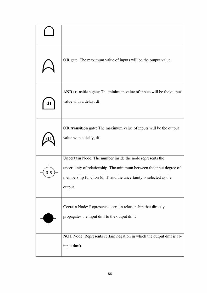
86  

OR gate: The maximum value of inputs will be the output value

AND transition gate: The minimum value of inputs will be the output

value with a delay, dt

OR transition gate: The maximum value of inputs will be the output

value with a delay, dt

Uncertain Node: The number inside the node represents the

uncertainty of relationship. The minimum between the input degree of

membership function (dmf) and the uncertainty is selected as the

output.

Certain Node: Represents a certain relationship that directly

propagates the input dmf to the output dmf.

NOT Node: Represents certain negation in which the output dmf is (1-

input dmf).

 

87  

Uncertain Negation Node: A hollow node with a bar above the

degree of certainty inside. The output dmf is the minimum between the

uncertainty and (1- input dmf).

Independent Node: Represents no relationship

Dependent Node: Represents that more DMLD hierarchies are

required to model the system behavior in details.

 

88  

Appendix B

Definitions of Bayesian Belief Network [8]

Acyclic Graph A graph that contains no cycles. At most one path

exists between each pair of nodes in the graph

Anticipatory node A leaf node that has not been instantiated. It is a node

awaiting evidence.

Arc A link or edge joining between 2 nodes.

Bayesian

Probabilities

Probabilities that are based on a person’s belief/expert

judgment of the likelihood of an event.

Belief The probability that a variable will be in a certain

state based on additional evidence in a current

situation of each possible state of a variable after

considering all available evidence.

A-priori beliefs are special case of beliefs that are

based only on prior information. A-priori beliefs are

determined only by the information stored in the

belief networks’ CPT [6]

Belief Network A graphical representation of a model that captures

the relationships between the model’s variables.

Binary variable A variable that has only two possible states.

Child A descendent variable whose state is directly

influenced by the parent variable.

 

89  

Clique A set of variables that are all pairwise linked.

Cluster tree A tree in which each node is a cluster of variables

from the domain of interest and each variable in the

domain appears in at least one node of the cluster

tree.

Clustering A technique where variables are grouped into clusters

to form singly connected network/trees.

Conditional

Probabilities

Conditional probabilities represent likelihoods based on prior information or past experience. [6]

Cyclic graph A graph that contains at least one cycle. This means

that multiple paths must exist between at least two of

the nodes in the graph.

D-Separation The blocking of the flow of evidence between nodes

or set of nodes in a network. It is used to represent

independence in causal belief network.

Decomposable model A probability model with a minimal independency

map.

Dependency map A graph in which all connected nodes correspond to

dependent variables in the model that is represented

Directed Acyclic

Graph

A graph that has direct arcs and no cycles.

Directed graph A graph containing directed arcs between nodes.

Dummy node A node representing evidence that bears upon another

node of interest.

Evidence It is information about a current situation [6]

 

90  

Evidence node A node with a single value that has been observed

with probability one.

Graph A set of nodes or vertices connected by a set of arcs

or edges.

Hypothesis node A node whose state represents one of a number of

alternative hypotheses

Inference The calculation of posterior marginal distributions for

variables of interests given a set of observations or

evidence.

Intermediate node A node inserted before a hypothesis variable to allow

uncertainty to be modeled.

Join tree A tree structure in which the nodes are the cliques of

the graph that it represents.

Leaf node A node whose arcs are directed towards it.

Likelihood How often a particular event is expected to occur.

Markov networks Graphical networks that are represented by undirected

graphs.

Marginal

distribution [5]

This distribution can be viewed as a projection of the

joint distribution on the smaller set of variables X1...

Xm.

Where

Maximal clique A maximal set of variables that are all pairwise

linked.

Neighbors Nodes that are directly connected to a node

 

91  

Parent A parent of a variable is any other variable that

directly influences the state of that variable.

Probabilistic Model An encoding of probabilistic information that allows

computation of every well formed

sentence/proposition in accordance with axioms of

the probability language.

Root node A node whose arcs are directed away from it.

Stochastic simulation A technique for computing probabilities by

measuring how frequently specific events occur

during simulation runs.

Uncertain evidence Specific evidence that do not directly identify the

state of a variable.

Undirected graph A graph that has arcs with no direction. i.e. Arcs that

exhibit bidirectional influence between nodes

Universe The set of all variables in a model representing all

knowledge in the domain of interest.

 

 

 

92  

Appendix C

 

MATLAB source code1: Pump System Model Application

 

function PumpSystem()

clc

clear all

close all

format long

%Defining input and output parameter range

x_GPM = 0:1:480; %Estimated Pump GPM range

x_Temp = 0:1:200; %Estimated Temperature range

x_Zo = 0:0.1:5; %Estmated Height of Pump range

x_NPSHA1 = 0:0.1:40; %Estimated NPSHA(Zo=0)range

x_NPSHA = 0:0.1:45; % Estimated NPSHA output

GPMmax = 480;

TempMax = 200;

 

93  

ZoMax = 10;

GPM_mu1 = 240; %Estimated GPM mean

GPM_sd1 = 80; %GPM standard deviation

Temp_mu1 = 100; %Estimated Temperature mean

Temp_sd1 = 30; %Temperature standard deviation

Zo_mu1 = 2.5; %Estimated Zo mean

Zo_sd1 = 0.8; %Zo standard deviation

N = 5000; %Sample Size

%Consider Monte Carlo Sampling based on a Uniform Distribution (Not used in

%Thesis example)

for i = 1:N

U_GPM(i) = GPMmax * rand(1); %Based on a uniform distribution input

U_Temp(i) = TempMax * rand(1); %Based on a uniform distribution input

U_Zo(i) = ZoMax * rand(1); %Based on a uniform distribution input

U_NPSHA1 = 35.18 - 6.4*10^-5 * U_GPM.^2 - 0.085 * U_Temp; %for Zo = 0

U_NPSHA = 35.18 + U_Zo - 6.4*10^-5 * U_GPM.^2 - 0.085 * U_Temp; %

NPSHA inclusive of Zo component.

end

 

94  

figure(1)

hist(U_NPSHA1,100) % Histogram of Uniform NPSHA1

xlabel('NPSHA1') % X Axis Label

ylabel('Number of Samples') % Y Axis Label

title('Histogram Plot of Uniform NPSHA')

[U_NPSHA1_mu U_NPSHA1_sd] = normfit(U_NPSHA1,0.05) %Calculate

mean and standard deviation of NPSHA1

U_NPSHA1_pdf = normpdf(x_NPSHA1,U_NPSHA1_mu, U_NPSHA1_sd); %pdf

of Uniform NPSHA1

U_NPSHA1_cdf = normcdf(x_NPSHA1,U_NPSHA1_mu, U_NPSHA1_sd); %cdf

of Uniform NPSHA1

figure(2)

plot(x_NPSHA1, U_NPSHA1_pdf, 'b') %Plot pdf of Uniform NPSHA1

xlabel('NPSHA1') % X Axis Label

ylabel('probability') % Y Axis Label

title('PDF Plot of U_NPSHA')

figure(3)

plot(x_NPSHA1, U_NPSHA1_cdf, 'r') %Plot cdf of Uniform NPSHA1

xlabel('NPSHA1') % X Axis Label

ylabel('probability') % Y Axis Label

title('CDF Plot of U_NPSHA')

 

95  

%Consider Monte Carlo Sampling for a normal distribution

for j = 1:N

N_GPM(j) = normrnd(GPM_mu1,GPM_sd1); %Based on a normal

distribution input

N_Temp(j) = normrnd(Temp_mu1,Temp_sd1); %Based on a normal distribution

input

N_Zo(j) = normrnd(Zo_mu1,Zo_sd1); %Based on a normal distribution input

N_NPSHA1 = 35.18 - 6.4*10^-5 * N_GPM.^2 - 0.085 * N_Temp; %For Zo = 0

N_NPSHA = 35.18 + N_Zo - 6.4*10^-5 * N_GPM.^2 - 0.085 * N_Temp; %

NPSHA inclusive of Zo component.

end

figure(4)

hist(N_NPSHA1,100) % Histogram for normal NPSHA1

xlabel('NPSHA1') % X Axis Label

ylabel('Number of Samples') % Y Axis Label

title('Histogram Plot of N_NPSHA')

[N_NPSHA1_mu N_NPSHA1_sd] = normfit(N_NPSHA1,0.05) %Calculate

mean and standard deviation of NPSHA1

N_NPSHA1_pdf = normpdf(x_NPSHA1,N_NPSHA1_mu, N_NPSHA1_sd); %pdf

of Normal NPSHA1

 

96  

N_NPSHA1_cdf = normcdf(x_NPSHA1,N_NPSHA1_mu, N_NPSHA1_sd); %cdf of

normal NPSHA1

[N_NPSHA_mu N_NPSHA_sd] = normfit(N_NPSHA,0.05) %Calculate mean

and standard deviation of NPSHA

N_NPSHA_pdf = normpdf(x_NPSHA,N_NPSHA_mu, N_NPSHA_sd); %pdf of

Normal NPSHA

N_NPSHA_cdf = normcdf(x_NPSHA,N_NPSHA_mu, N_NPSHA_sd); %cdf of

Normal NPSHA

[N_Temp_mu, N_Temp_sd] = normfit (N_Temp,0.05); %Calculate mean and

standard deviation of Temperature

N_Temp_pdf = normpdf(x_Temp,N_Temp_mu,N_Temp_sd); %pdf of Normal

Temperature

N_Temp_cdf = normcdf(x_Temp,N_Temp_mu,N_Temp_sd); %cdf of Normal

Temperature

LWTempdata = N_Temp_cdf(100) %Estimating the probabililty of Low

Temperature data

HITempdata = N_Temp_cdf(200) - N_Temp_cdf(100) %Estimating the probability

of High Temperature data

 

97  

figure(5)

plot(x_NPSHA1, N_NPSHA1_pdf, 'b')

xlabel('NPSHA1') % X Axis Label

ylabel('frequency') % Y Axis Label

title('PDF Plot of N_NPSHA1')

figure(6)

plot(x_NPSHA1, N_NPSHA1_cdf, 'r')

xlabel('NPSHA1') % X Axis Label

ylabel('probability') % Y Axis Label

title('CDF Plot of N_NPSHA1')

[n1,xout1] = hist(N_NPSHA1,12); %breaking down the normal distribution into 12

parts

norm_den1 = sum(n1)* (max(N_NPSHA1)-min(N_NPSHA1))/12;

figure(7);

bar(xout1,n1/norm_den1,'hist');hold on;

plot(x_NPSHA1, N_NPSHA1_pdf, 'r')

xlabel('NPSHA1') % X Axis Label

ylabel('frequency') % Y Axis Label

title('PDF Plot of N_NPSHA1 with Histogram')

I = 12;

max_Xout1 = max(N_NPSHA1) %estimating the maximum NPSHA1

 

98  

min_Xout1 = min(N_NPSHA1) %estimating the minimum NPSHA1

Interval1 = (max_Xout1 - min_Xout1)/I;

Amax = min_Xout1 + Interval1

Bmax = Amax + Interval1

Cmax = Bmax + Interval1

Dmax = Cmax + Interval1

Emax = Dmax + Interval1

Fmax = Emax + Interval1

Gmax = Fmax + Interval1

Hmax = Gmax + Interval1

Imax = Hmax + Interval1

Jmax = Imax + Interval1

Kmax = Jmax + Interval1

Lmax = Kmax + Interval1

%Obtaining Probability Data from Physical Model assuming no overlaps

Aact = normcdf(Amax, N_NPSHA1_mu, N_NPSHA1_sd)

Bact = normcdf(Bmax, N_NPSHA1_mu, N_NPSHA1_sd) - normcdf(Amax,

N_NPSHA1_mu, N_NPSHA1_sd)

Cact = normcdf(Cmax, N_NPSHA1_mu, N_NPSHA1_sd) - normcdf(Bmax,

N_NPSHA1_mu, N_NPSHA1_sd)

Dact = normcdf(Dmax, N_NPSHA1_mu, N_NPSHA1_sd) - normcdf(Cmax,

N_NPSHA1_mu, N_NPSHA1_sd)

 

99  

Eact = normcdf(Emax, N_NPSHA1_mu, N_NPSHA1_sd) - normcdf(Dmax,

N_NPSHA1_mu, N_NPSHA1_sd)

Fact = normcdf(Fmax, N_NPSHA1_mu, N_NPSHA1_sd) - normcdf(Emax,

N_NPSHA1_mu, N_NPSHA1_sd)

Gact = normcdf(Gmax, N_NPSHA1_mu, N_NPSHA1_sd) - normcdf(Fmax,

N_NPSHA1_mu, N_NPSHA1_sd)

Hact = normcdf(Hmax, N_NPSHA1_mu, N_NPSHA1_sd) - normcdf(Gmax,

N_NPSHA1_mu, N_NPSHA1_sd)

Iact = normcdf(Imax, N_NPSHA1_mu, N_NPSHA1_sd) - normcdf(Hmax,

N_NPSHA1_mu, N_NPSHA1_sd)

Jact = normcdf(Jmax, N_NPSHA1_mu, N_NPSHA1_sd) - normcdf(Imax,

N_NPSHA1_mu, N_NPSHA1_sd)

Kact = normcdf(Kmax, N_NPSHA1_mu, N_NPSHA1_sd) - normcdf(Jmax,

N_NPSHA1_mu, N_NPSHA1_sd)

Lact = normcdf(Lmax, N_NPSHA1_mu, N_NPSHA1_sd) - normcdf(Kmax,

N_NPSHA1_mu, N_NPSHA1_sd)

[n,xout] = hist(N_NPSHA,4);

norm_den = sum(n)* (max(N_NPSHA)-min(N_NPSHA))/4;

figure(8);

bar(xout,n/norm_den,'hist');hold on;

plot(x_NPSHA, N_NPSHA_pdf, 'r')

xlabel('NPSHA') % X Axis Label

ylabel('frequency') % Y Axis Label

title('PDF Plot of N_NPSHA with Histogram')

 

100  

I = 4;

max_Xout = max(N_NPSHA);

min_Xout = min(N_NPSHA);

Interval1 = (max_Xout-min_Xout)/I;

Mmax = min_Xout + Interval1;

Nmax = Mmax + Interval1;

Omax = Nmax + Interval1;

Pmax = Omax + Interval1;

%Estimating the probability of M, N, O, P

M = normcdf(Mmax, N_NPSHA_mu, N_NPSHA_sd)

N = normcdf(Nmax, N_NPSHA_mu, N_NPSHA_sd) - normcdf(Mmax,

N_NPSHA_mu, N_NPSHA_sd)

O = normcdf(Omax, N_NPSHA_mu, N_NPSHA_sd) - normcdf(Nmax,

N_NPSHA_mu, N_NPSHA_sd)

P = normcdf(Pmax, N_NPSHA_mu, N_NPSHA_sd) - normcdf(Omax,

N_NPSHA_mu, N_NPSHA_sd)

[N_GPM_mu ,N_GPM_sd] = normfit (N_GPM,0.05); %Calculating the mean and

standard deviation of GPM

N_GPM_pdf = normpdf(x_GPM ,N_GPM_mu,N_GPM_sd); %pdf of GPM

N_GPM_cdf = normcdf(x_GPM ,N_GPM_mu,N_GPM_sd); %cdf of GPM

 

101  

[N_Zo_mu, N_Zo_sd] = normfit (N_Zo,0.05); %Calculating the mean and

standard deviation of Zo

N_Zo_pdf = normpdf(x_Zo,N_Zo_mu,N_Zo_sd); %pdf of Zo

N_Zo_cdf = normcdf(x_Zo,N_Zo_mu,N_Zo_sd); %cdf of Zo

figure(9)

plot(x_GPM, N_GPM_pdf, 'r')

xlabel('GPM') % X Axis Label

ylabel('frequency') % Y Axis Label

title('PDF Plot of GPM')

figure(10)

plot(x_Temp, N_Temp_pdf, 'b')

xlabel('Temp') % X Axis Label

ylabel('frequency') % Y Axis Label

title('PDF Plot of Temp')

figure(11)

plot(x_Zo, N_Zo_pdf, 'b')

xlabel('Zo') % X Axis Label

ylabel('frequency') % Y Axis Label

title('PDF Plot of Zo')

 

102  

figure(12)

plot(x_Temp, N_Temp_cdf, 'b')

xlabel('Temp') % X Axis Label

ylabel('Probability') % Y Axis Label

title('CDF Plot of Temp')

figure(13)

plot(x_GPM, N_GPM_cdf, 'r')

xlabel('GPM') % X Axis Label

ylabel('probability') % Y Axis Label

title('CDF Plot of GPM')

figure(14)

plot(x_Zo, N_Zo_cdf, 'r')

xlabel('Zo') % X Axis Label

ylabel('probability') % Y Axis Label

title('CDF Plot of Zo')

%Estimating the probability of individual Temperature states

LWTempdata = N_Temp_cdf(100)

HITempdata = N_Temp_cdf(200) - N_Temp_cdf(100)

%Estimating the probability of individual GPM states

ZE_GPMdata = normcdf(1, N_GPM_mu,N_GPM_sd)

 

103  

LW_GPMdata = normcdf(90, N_GPM_mu,N_GPM_sd) - normcdf(1,

N_GPM_mu,N_GPM_sd)

ML_GPMdata = normcdf(180, N_GPM_mu,N_GPM_sd) - normcdf(90,

N_GPM_mu,N_GPM_sd)

MD_GPMdata = normcdf(300, N_GPM_mu,N_GPM_sd) - normcdf(180,

N_GPM_mu,N_GPM_sd)

MH_GPMdata = normcdf(390, N_GPM_mu,N_GPM_sd) - normcdf(300,

N_GPM_mu,N_GPM_sd)

HI_GPMdata = normcdf(480, N_GPM_mu,N_GPM_sd) - normcdf(390,

N_GPM_mu,N_GPM_sd)

%Estimating the probability of individual Zo states

N_ZoNE = normcdf(2.5,N_Zo_mu,N_Zo_sd)

N_ZoPT = normcdf(5,N_Zo_mu,N_Zo_sd) - normcdf(2.5,N_Zo_mu,N_Zo_sd)

% Bayesian Belief Network Methodology

S1 = HI_GPMdata * HITempdata

S2 = MH_GPMdata * HITempdata

S3 = MD_GPMdata * HITempdata

S4 = ML_GPMdata * HITempdata

S5 = LW_GPMdata * HITempdata

S6 = ZE_GPMdata * HITempdata

S7 = HI_GPMdata * LWTempdata

S8 = MH_GPMdata * LWTempdata

S9 = MD_GPMdata * LWTempdata

 

104  

S10 = ML_GPMdata * LWTempdata

S11 = LW_GPMdata * LWTempdata

S12 = ZE_GPMdata * LWTempdata

SUM = S1 + S2 + S3 + S4 + S5 + S6 + S7 + S8 + S9 + S10 + S11 + S12

end

MATLAB Source Code 2: Comparison of NPSHA1 data between Physical and Fuzzy Logic Model

%Comparison of NPSHA data between physical model and Fuzzy Logic Model

%Fuzzy Interface System was used to generate the Fuzzy output.

clc % clears all input and output from command window

clear all % clears the values stored in all variables

%close all % closes all MatLab figures open in Windows

fis = readfis('Pump System2');

surfview(fis) %Surface view of NPSHA with respect to Temperature and Pump

GPM

 

105  

%Estimating NPSHA output at Temperature = 0degF between GPM 0 to 480

out0deg = evalfis([0 0 0 0 0 0 0 0 0 0 0 0 0 0 0 0 0 0 0 0 0 0 0 0 0 ;0 20 40 60 80 100

120 140 160 180 ...

200 220 240 260 280 300 320 340 360 380 400 420 440 460 480],fis)

%Estimating NPSHA output at Temperature = 40degF between GPM 0 to 480

out40deg = evalfis([40 40 40 40 40 40 40 40 40 40 40 40 40 40 40 40 40 40 40 40 40

40 40 40 40 ;0 20 40 60 80 100 120 140 160 180 ...

200 220 240 260 280 300 320 340 360 380 400 420 440 460 480],fis)

%Estimating NPSHA output at Temperature = 80degF between GPM 0 to 480

out80deg = evalfis([80 80 80 80 80 80 80 80 80 80 80 80 80 80 80 80 80 80 80 80 80

80 80 80 80 ;0 20 40 60 80 100 120 140 160 180 ...

200 220 240 260 280 300 320 340 360 380 400 420 440 460 480],fis)

%Estimating NPSHA output at Temperature = 120degF between GPM 0 to 480

out120deg = evalfis([120 120 120 120 120 120 120 120 120 120 120 120 120 120

120 120 120 120 120 120 120 120 120 120 120 ;0 ...

20 40 60 80 100 120 140 160 180 200 220 240 260 280 300 320 340 360 380 400

420 440 460 480],fis)

%Estimating NPSHA output at Temperature = 160degF between GPM 0 to 480

out160deg = evalfis([160 160 160 160 160 160 160 160 160 160 160 160 160 160

160 160 160 160 160 160 160 160 160 160 160 ;0 ...

 

106  

20 40 60 80 100 120 140 160 180 200 220 240 260 280 300 320 340 360 380 400

420 440 460 480],fis)

%Estimating NPSHA output at Temperature = 2000degF between GPM 0 to 480

out200deg = evalfis([200 200 200 200 200 200 200 200 200 200 200 200 200 200

200 200 200 200 200 200 200 200 200 200 200 ;0 ...

20 40 60 80 100 120 140 160 180 200 220 240 260 280 300 320 340 360 380 400

420 440 460 480],fis)

%Plotting Fuzzy NPSHA output vs Pump GPM at 6 different temperatures

GPM = 0 :20: 480;

figure(10)

hold on;

plot(GPM, out0deg, 'r')

plot(GPM, out40deg, 'b')

plot(GPM, out80deg, 'g')

plot(GPM, out120deg, 'k')

plot(GPM, out160deg, 'm')

plot(GPM, out200deg, 'c')

title('Fuzzy NPSHA Vs Fuzzy PUMP GPM (Zo=0)')

legend('fT=0', 'fT=40', 'fT=80', 'fT=120', 'fT=160', 'fT=200')

xlabel('PUMP GPM') %X axis

ylabel('NPSHA1') %Y axis

 

107  

%Plotting Physical NPSHA output vs Pump GPM at 6 different temperatures

for Z0 = 0

GPM = 0: 1 : 480;

%figure(11)

TEMP=0;

plot(GPM, 35.18 + Z0 - 6.4*10^-5 * GPM.^2 - 0.085 * TEMP,'-- r')

hold on;

TEMP = 40;

plot(GPM, 35.18 + Z0 - 6.4*10^-5 * GPM.^2 - 0.085 * TEMP,'-- b')

TEMP = 80;

plot(GPM, 35.18 + Z0 - 6.4*10^-5 * GPM.^2 - 0.085 * TEMP,'-- g')

TEMP = 120;

plot(GPM, 35.18 + Z0 - 6.4*10^-5 * GPM.^2 - 0.085 * TEMP,'-- k')

TEMP = 160;

plot(GPM, 35.18 + Z0 - 6.4*10^-5 * GPM.^2 - 0.085 * TEMP,'-- m' )

TEMP = 200;

plot(GPM, 35.18 + Z0 - 6.4*10^-5 * GPM.^2 - 0.085 * TEMP,'-- c')

title('NPSHA Vs PUMP GPM (Zo=0)')

legend('T=0', 'T=40', 'T=80', 'T=120', 'T=160', 'T=200')

xlabel('PUMP GPM') %X axis

ylabel('NPSHA') %Y axis

hold off

end

 

108  

MATLAB Source Code 3: Distribution of NPSHA1 output

%Distribution of NPSHA1 at various GPM and Temperature range

%S1 to S2 is assumed to be normally distributed across the A to L range

%Overlaps between the normal distributions would be accounted for

function NPSHA1output()

clc

clear all

close all

format long

%Initial estimated ranges of A to L

x_A = 2:0.1:17;

x_B = 7:0.1: 22;

x_C = 11:0.1:26;

x_D = 15:0.1:27;

x_E = 16:0.1:28;

x_F = 17:0.1:28;

x_G = 10:0.1:27;

x_H = 15:0.1:31;

x_I = 19:0.1:34;

x_J = 24:0.1:35;

x_K = 25:0.1:37;

x_L = 25: 0.1:37;

 

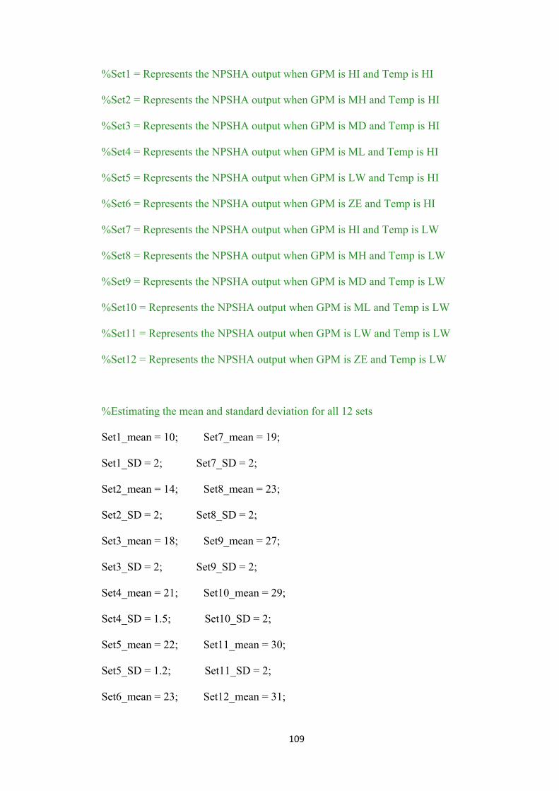
109  

%Set1 = Represents the NPSHA output when GPM is HI and Temp is HI

%Set2 = Represents the NPSHA output when GPM is MH and Temp is HI

%Set3 = Represents the NPSHA output when GPM is MD and Temp is HI

%Set4 = Represents the NPSHA output when GPM is ML and Temp is HI

%Set5 = Represents the NPSHA output when GPM is LW and Temp is HI

%Set6 = Represents the NPSHA output when GPM is ZE and Temp is HI

%Set7 = Represents the NPSHA output when GPM is HI and Temp is LW

%Set8 = Represents the NPSHA output when GPM is MH and Temp is LW

%Set9 = Represents the NPSHA output when GPM is MD and Temp is LW

%Set10 = Represents the NPSHA output when GPM is ML and Temp is LW

%Set11 = Represents the NPSHA output when GPM is LW and Temp is LW

%Set12 = Represents the NPSHA output when GPM is ZE and Temp is LW

%Estimating the mean and standard deviation for all 12 sets

Set1_mean = 10; Set7_mean = 19;

Set1_SD = 2; Set7_SD = 2;

Set2_mean = 14; Set8_mean = 23;

Set2_SD = 2; Set8_SD = 2;

Set3_mean = 18; Set9_mean = 27;

Set3_SD = 2; Set9_SD = 2;

Set4_mean = 21; Set10_mean = 29;

Set4_SD = 1.5; Set10_SD = 2;

Set5_mean = 22; Set11_mean = 30;

Set5_SD = 1.2; Set11_SD = 2;

Set6_mean = 23; Set12_mean = 31;

 

110  

Set6_SD = 1.2; Set12_SD = 1.5;

N = 5000;

%Normal Random Sampling of A to L based on 5000 samples

for j = 1:N

A(j) = normrnd(Set1_mean,Set1_SD);

B(j) = normrnd(Set2_mean,Set2_SD);

C(j) = normrnd(Set3_mean,Set3_SD);

D(j) = normrnd(Set4_mean,Set4_SD);

E(j) = normrnd(Set5_mean,Set5_SD);

F(j) = normrnd(Set6_mean,Set6_SD);

G(j) = normrnd(Set7_mean,Set7_SD);

H(j) = normrnd(Set8_mean,Set8_SD);

I(j) = normrnd(Set9_mean,Set9_SD);

J(j) = normrnd(Set10_mean,Set10_SD);

K(j) = normrnd(Set11_mean,Set11_SD);

L(j) = normrnd(Set12_mean,Set12_SD);

end

%Defining Probability Input Paramenters obtained from PumpSystemFinal.m

LWTempdata = 0.491593887090371;

HITempdata = 0.507981643183724;

 

111  

HI_GPMdata = 0.030244034122316;

MH_GPMdata = 0.199614391751596;

MD_GPMdata = 0.545470490189395;

ML_GPMdata = 0.193391376667252;

LW_GPMdata = 0.028448548042403;

ZE_GPMdata = 0.001382396691117;

S1 = HI_GPMdata * HITempdata;

S2 = MH_GPMdata * HITempdata;

S3 = MD_GPMdata * HITempdata;

S4 = ML_GPMdata * HITempdata;

S5 = LW_GPMdata * HITempdata;

S6 = ZE_GPMdata * HITempdata;

S7 = HI_GPMdata * LWTempdata;

S8 = MH_GPMdata * LWTempdata;

S9 = MD_GPMdata * LWTempdata;

S10 = ML_GPMdata * LWTempdata;

S11 = LW_GPMdata * LWTempdata;

S12 = ZE_GPMdata * LWTempdata;

[A_mu A_sd] = normfit(A,0.05);

A_pdf = normpdf(x_A,A_mu, A_sd);

A_cdf = normcdf(x_A,A_mu, A_sd);

 

112  

%Left Side Truncated Normal Distribution of A at 6.59

AT_pdf = normpdf(x_A,A_mu, A_sd)/(1-normcdf(6.59,A_mu,A_sd));

AT_cdf = (normcdf(x_A,A_mu, A_sd) - normcdf(6.59,A_mu, A_sd))/(1-

normcdf(6.59,A_mu,A_sd));

figure(1)

plot(x_A, A_pdf, 'b')

xlabel('NPSHA1') % X Axis Label

ylabel('frequency') % Y Axis Label

title('PDF Plot of Set1')

hold on;

plot(x_A, AT_pdf, 'r')

hold off;

figure(2)

plot(x_A, A_cdf, 'b')

xlabel('NPSHA1') % X Axis Label

ylabel('probability') % Y Axis Label

title('CDF Plot of Set1')

hold on;

plot(x_A, AT_cdf, 'r')

hold off;

 

113  

A1 = (normcdf(8.94312,A_mu, A_sd) - normcdf(6.59,A_mu, A_sd))/(1-

normcdf(6.59,A_mu,A_sd)) - ...

(normcdf(6.59,A_mu, A_sd) - normcdf(6.59,A_mu, A_sd))/(1-

normcdf(6.59,A_mu,A_sd))

A2 = (normcdf(11.29611,A_mu, A_sd) - normcdf(6.59,A_mu, A_sd))/(1-

normcdf(6.59,A_mu,A_sd)) - ...

(normcdf(8.94312,A_mu, A_sd) - normcdf(6.59,A_mu, A_sd))/(1-

normcdf(6.59,A_mu,A_sd))

A3 = (normcdf(13.6491,A_mu, A_sd) - normcdf(6.59,A_mu, A_sd))/(1-

normcdf(6.59,A_mu,A_sd)) - ...

(normcdf(11.29611,A_mu, A_sd) - normcdf(6.59,A_mu, A_sd))/(1-

normcdf(6.59,A_mu,A_sd))

A4 = (normcdf(16.002,A_mu, A_sd) - normcdf(6.59,A_mu, A_sd))/(1-

normcdf(6.59,A_mu,A_sd)) - ...

(normcdf(13.6491,A_mu, A_sd) - normcdf(6.59,A_mu, A_sd))/(1-

normcdf(6.59,A_mu,A_sd))

A5 = 1 - (normcdf(16.002,A_mu, A_sd) - normcdf(6.59,A_mu, A_sd))/(1-

normcdf(6.59,A_mu,A_sd))

SUMA =A1+A2+A3+A4+A5

 

114  

[B_mu B_sd] = normfit(B,0.05);

B_pdf = normpdf(x_B,B_mu, B_sd);

B_cdf = normcdf(x_B,B_mu, B_sd);

figure(3)

plot(x_B, B_pdf, 'b')

xlabel('NPSHA1') % X Axis Label

ylabel('frequency') % Y Axis Label

title('PDF Plot of Set2')

figure(4)

plot(x_B, B_cdf, 'r')

xlabel('NPSHA1') % X Axis Label

ylabel('probability') % Y Axis Label

title('CDF Plot of Set2')

B1 = normcdf(8.84312,B_mu, B_sd)

B2 = normcdf(11.2961,B_mu, B_sd) - normcdf(8.84312,B_mu, B_sd)

B3 = normcdf(13.6491,B_mu, B_sd) - normcdf(11.2961,B_mu, B_sd)

B4 = normcdf(16.002,B_mu, B_sd) - normcdf(13.6491,B_mu, B_sd)

B5 = normcdf(18.3551,B_mu, B_sd) - normcdf(16.002,B_mu, B_sd)

 

115  

B6 = normcdf(20.708,B_mu, B_sd) - normcdf(18.3551,B_mu, B_sd)

B7 = 1- normcdf(20.708,B_mu, B_sd)

SUMB = B1+B2+B3+B4+B5+B6+B7

[C_mu C_sd] = normfit(C,0.05);

C_pdf = normpdf(x_C,C_mu, C_sd);

C_cdf = normcdf(x_C,C_mu, C_sd);

figure(5)

plot(x_C, C_pdf, 'b')

xlabel('NPSHA1') % X Axis Label

ylabel('frequency') % Y Axis Label

title('PDF Plot of Set3')

figure(6)

plot(x_C, C_cdf, 'r')

xlabel('NPSHA1') % X Axis Label

ylabel('probability') % Y Axis Label

title('CDF Plot of Set3')

 

116  

C2 = normcdf(11.2961,C_mu, C_sd)

C3 = normcdf(13.6491,C_mu, C_sd) - normcdf(11.2961,C_mu, C_sd)

C4 = normcdf(16.002,C_mu, C_sd) - normcdf(13.6491,C_mu, C_sd)

C5 = normcdf(18.3551,C_mu, C_sd) - normcdf(16.002,C_mu, C_sd)

C6 = normcdf(20.708,C_mu, C_sd) - normcdf(18.3551,C_mu, C_sd)

C7 = normcdf(23.061,C_mu, C_sd) - normcdf(20.708,C_mu, C_sd)

C8 = 1- normcdf(23.061,C_mu, C_sd)

SUMC = C2+C3+C4+C5+C6+C7+C8

[D_mu D_sd] = normfit(D,0.05);

D_pdf = normpdf(x_D,D_mu, D_sd);

D_cdf = normcdf(x_D,D_mu, D_sd);

figure(7)

plot(x_D, D_pdf, 'b')

xlabel('NPSHA1') % X Axis Label

ylabel('frequency') % Y Axis Label

title('PDF Plot of Set4')

 

117  

figure(8)

plot(x_D, D_cdf, 'r')

xlabel('NPSHA1') % X Axis Label

ylabel('probability') % Y Axis Label

title('CDF Plot of Set4')

D4 = normcdf(16.002,D_mu, D_sd)

D5 = normcdf(18.3551,D_mu, D_sd) - normcdf(16.002,D_mu, D_sd)

D6 = normcdf(20.708,D_mu, D_sd) - normcdf(18.3551,D_mu, D_sd)

D7 = normcdf(23.061,D_mu, D_sd) - normcdf(20.708,D_mu, D_sd)

D8 = normcdf(25.41407,D_mu, D_sd) - normcdf(23.061,D_mu, D_sd)

D9 = 1- normcdf(25.41407,D_mu, D_sd)

SUMD =D4+D5+D6+D7+D8+D9

[E_mu E_sd] = normfit(E,0.05);

 

118  

E_pdf = normpdf(x_E,E_mu, E_sd);

E_cdf = normcdf(x_E,E_mu, E_sd);

figure(9)

plot(x_E, E_pdf, 'b')

xlabel('NPSHA1') % X Axis Label

ylabel('frequency') % Y Axis Label

title('PDF Plot of Set5')

figure(10)

plot(x_E, E_cdf, 'r')

xlabel('NPSHA1') % X Axis Label

ylabel('probability') % Y Axis Label

title('CDF Plot of Set5')

E4 = normcdf(16.002,E_mu, E_sd)

E5 = normcdf(18.3551,E_mu, E_sd) - normcdf(16.002,E_mu, E_sd)

E6 = normcdf(20.708,E_mu, E_sd) - normcdf(18.3551,E_mu, E_sd)

E7 = normcdf(23.061,E_mu, E_sd) - normcdf(20.708,E_mu, E_sd)

E8 = normcdf(25.41407,E_mu, E_sd) - normcdf(23.061,E_mu, E_sd)

 

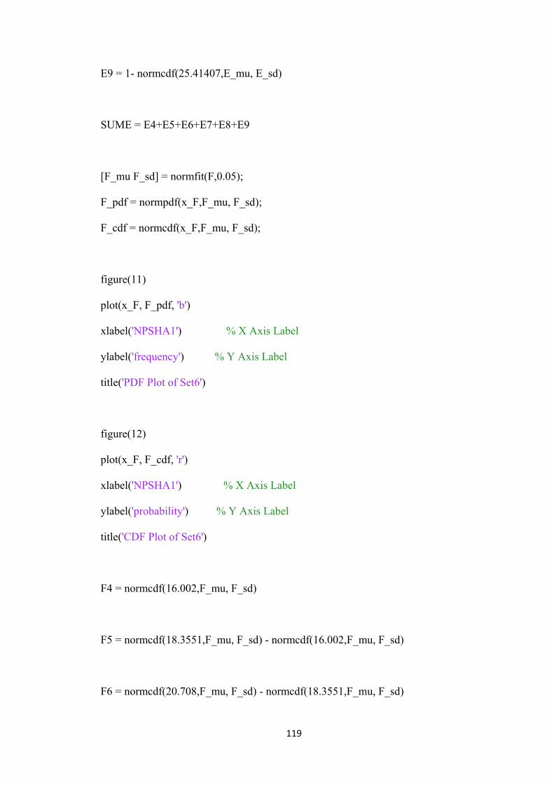
119  

E9 = 1- normcdf(25.41407,E_mu, E_sd)

SUME = E4+E5+E6+E7+E8+E9

[F_mu F_sd] = normfit(F,0.05);

F_pdf = normpdf(x_F,F_mu, F_sd);

F_cdf = normcdf(x_F,F_mu, F_sd);

figure(11)

plot(x_F, F_pdf, 'b')

xlabel('NPSHA1') % X Axis Label

ylabel('frequency') % Y Axis Label

title('PDF Plot of Set6')

figure(12)

plot(x_F, F_cdf, 'r')

xlabel('NPSHA1') % X Axis Label

ylabel('probability') % Y Axis Label

title('CDF Plot of Set6')

F4 = normcdf(16.002,F_mu, F_sd)

F5 = normcdf(18.3551,F_mu, F_sd) - normcdf(16.002,F_mu, F_sd)

F6 = normcdf(20.708,F_mu, F_sd) - normcdf(18.3551,F_mu, F_sd)

 

120  

F7 = normcdf(23.061,F_mu, F_sd) - normcdf(20.708,F_mu, F_sd)

F8 = normcdf(25.41407,F_mu, F_sd) - normcdf(23.061,F_mu, F_sd)

F9 = 1- normcdf(25.41407,F_mu, F_sd)

SUMF = F4+F5+F6+F7+F8+F9

[G_mu G_sd] = normfit(G,0.05);

G_pdf = normpdf(x_G,G_mu, G_sd);

G_cdf = normcdf(x_G,G_mu, G_sd);

figure(13)

plot(x_G, G_pdf, 'b')

xlabel('NPSHA1') % X Axis Label

ylabel('frequency') % Y Axis Label

title('PDF Plot of Set7')

figure(14)

plot(x_G, G_cdf, 'r')

xlabel('NPSHA1') % X Axis Label

ylabel('probability') % Y Axis Label

title('CDF Plot of Set7')

 

121  

G2 = normcdf(11.2961,G_mu, G_sd)

G3 = normcdf(13.6491,G_mu, G_sd) - normcdf(11.2961,G_mu, G_sd)

G4 = normcdf(16.002,G_mu, G_sd) - normcdf(13.6491,G_mu, G_sd)

G5 = normcdf(18.3551,G_mu, G_sd) - normcdf(16.002,G_mu, G_sd)

G6 = normcdf(20.708,G_mu, G_sd) - normcdf(18.3551,G_mu, G_sd)

G7 = normcdf(23.061,G_mu, G_sd) - normcdf(20.708,G_mu, G_sd)

G8 = 1- normcdf(23.061,G_mu, G_sd)

SUMG = G2+G3+G4+G5+G6+G7+G8

[H_mu H_sd] = normfit(H,0.05);

H_pdf = normpdf(x_H,H_mu, H_sd);

H_cdf = normcdf(x_H,H_mu, H_sd);

figure(15)

plot(x_H, H_pdf, 'b')

xlabel('NPSHA1') % X Axis Label

ylabel('frequency') % Y Axis Label

title('PDF Plot of Set8')

 

122  

figure(16)

plot(x_H, H_cdf, 'r')

xlabel('NPSHA1') % X Axis Label

ylabel('probability') % Y Axis Label

title('CDF Plot of Set8')

H4 = normcdf(16.002,H_mu, H_sd)

H5 = normcdf(18.3551,H_mu, H_sd) - normcdf(16.002,H_mu, H_sd)

H6 = normcdf(20.708,H_mu, H_sd) - normcdf(18.3551,H_mu, H_sd)

H7 = normcdf(23.061,H_mu, H_sd) - normcdf(20.708,H_mu, H_sd)

H8 = normcdf(25.41407,H_mu, H_sd) - normcdf(23.061,H_mu, H_sd)

H9 = normcdf(27.767,H_mu, H_sd) - normcdf(25.41407,H_mu, H_sd)

H10 = 1- normcdf(27.767,H_mu, H_sd)

SUMH = H4+H5+H6+H7+H8+H9+H10

[I_mu I_sd] = normfit(I,0.05);

I_pdf = normpdf(x_I,I_mu, I_sd);

 

123  

I_cdf = normcdf(x_I,I_mu, I_sd);

figure(17)

plot(x_I, I_pdf, 'b')

xlabel('NPSHA1') % X Axis Label

ylabel('frequency') % Y Axis Label

title('PDF Plot of Set9')

figure(18)

plot(x_I, I_cdf, 'r')

xlabel('NPSHA1') % X Axis Label

ylabel('probability') % Y Axis Label

title('CDF Plot of Set9')

I6 = normcdf(20.708,I_mu, I_sd) - normcdf(18.3551,I_mu, I_sd)

I7 = normcdf(23.061,I_mu, I_sd) - normcdf(20.708,I_mu, I_sd)

I8 = normcdf(25.41407,I_mu, I_sd) - normcdf(23.061,I_mu, I_sd)

I9 = normcdf(27.767,I_mu, I_sd) - normcdf(25.41407,I_mu, I_sd)

I10 = normcdf(30.12,I_mu, I_sd) - normcdf(27.767,I_mu, I_sd)

I11 = normcdf(32.473,I_mu, I_sd) - normcdf(30.12,I_mu, I_sd)

 

124  

I12 = 1- normcdf(32.473,I_mu, I_sd)

SUMI = I6+I7+I8+I9+I10+I11+I12

[J_mu J_sd] = normfit(J,0.05);

J_pdf = normpdf(x_J,J_mu, J_sd);

J_cdf = normcdf(x_J,J_mu, J_sd);

figure(19)

plot(x_J, J_pdf, 'b')

xlabel('NPSHA1') % X Axis Label

ylabel('frequency') % Y Axis Label

title('PDF Plot of Set10')

figure(20)

plot(x_J, J_cdf, 'r')

xlabel('NPSHA1') % X Axis Label

ylabel('probability') % Y Axis Label

title('CDF Plot of Set10')

J7 = normcdf(23.061,J_mu, J_sd) - normcdf(20.708,J_mu, J_sd)

J8 = normcdf(25.41407,J_mu, J_sd) - normcdf(23.061,J_mu, J_sd)

J9 = normcdf(27.767,J_mu, J_sd) - normcdf(25.41407,J_mu, J_sd)

 

125  

J10 = normcdf(30.12,J_mu, J_sd) - normcdf(27.767,J_mu, J_sd)

J11 = normcdf(32.473,J_mu, J_sd) - normcdf(30.12,J_mu, J_sd)

J12 = 1- normcdf(32.473,J_mu, J_sd)

SUMJ = J7+J8+J9+J10+J11+J12

[K_mu K_sd] = normfit(K,0.05);

K_pdf = normpdf(x_K,K_mu, K_sd);

K_cdf = normcdf(x_K,K_mu, K_sd);

figure(21)

plot(x_K, K_pdf, 'b')

xlabel('NPSHA1') % X Axis Label

ylabel('frequency') % Y Axis Label

title('PDF Plot of Set11')

figure(22)

plot(x_K, K_cdf, 'r')

xlabel('NPSHA1') % X Axis Label

ylabel('probability') % Y Axis Label

title('CDF Plot of Set11')

 

126  

K8 = normcdf(25.41407,K_mu, K_sd) - normcdf(23.061,K_mu, K_sd)

K9 = normcdf(27.767,K_mu, K_sd) - normcdf(25.41407,K_mu, K_sd)

K10 = normcdf(30.12,K_mu, K_sd) - normcdf(27.767,K_mu, K_sd)

K11 = normcdf(32.473,K_mu, K_sd) - normcdf(30.12,K_mu, K_sd)

K12 = 1- normcdf(32.473,K_mu, K_sd)

SUMK = K8+K9+K10+K11+K12

[L_mu L_sd] = normfit(L,0.05);

L_pdf = normpdf(x_L,L_mu, L_sd);

L_cdf = normcdf(x_L,L_mu, L_sd);

%Right Side Truncated Normal Distribution of L at 34.826

LT_pdf = normpdf(x_L,L_mu, L_sd)/normcdf(34.826,L_mu,L_sd);

LT_cdf = normcdf(x_L,L_mu, L_sd)/normcdf(34.826,L_mu,L_sd);

figure(23)

plot(x_L, L_pdf, 'b')

xlabel('NPSHA1') % X Axis Label

 

127  

ylabel('frequency') % Y Axis Label

title('PDF Plot of Set12')

hold on;

plot(x_L, LT_pdf, 'r')

hold off;

figure(24)

plot(x_L, L_cdf, 'b')

xlabel('NPSHA1') % X Axis Label

ylabel('probability') % Y Axis Label

title('CDF Plot of Set12')

hold on;

plot(x_L, LT_cdf, 'r')

hold off;

L8 = normcdf(25.414 ,L_mu, L_sd)/normcdf(34.826,L_mu,L_sd)

L9 = normcdf(27.767 ,L_mu, L_sd)/normcdf(34.826,L_mu,L_sd) - normcdf(25.414

,L_mu, L_sd)/normcdf(34.826,L_mu,L_sd)

L10 = normcdf(30.12 ,L_mu, L_sd)/normcdf(34.826,L_mu,L_sd) - normcdf(27.767

,L_mu, L_sd)/normcdf(34.826,L_mu,L_sd)

L11 = normcdf(32.826 ,L_mu, L_sd)/normcdf(34.826,L_mu,L_sd) - normcdf(30.12

,L_mu, L_sd)/normcdf(34.826,L_mu,L_sd)

 

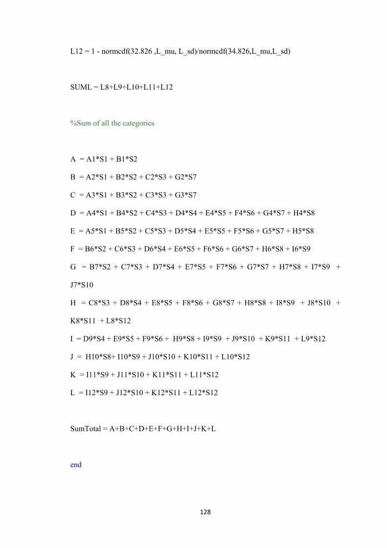
128  

L12 = 1 - normcdf(32.826 ,L_mu, L_sd)/normcdf(34.826,L_mu,L_sd)

SUML = L8+L9+L10+L11+L12

%Sum of all the categories

A = A1*S1 + B1*S2

B = A2*S1 + B2*S2 + C2*S3 + G2*S7

C = A3*S1 + B3*S2 + C3*S3 + G3*S7

D = A4*S1 + B4*S2 + C4*S3 + D4*S4 + E4*S5 + F4*S6 + G4*S7 + H4*S8

E = A5*S1 + B5*S2 + C5*S3 + D5*S4 + E5*S5 + F5*S6 + G5*S7 + H5*S8

F = B6*S2 + C6*S3 + D6*S4 + E6*S5 + F6*S6 + G6*S7 + H6*S8 + I6*S9

G = B7*S2 + C7*S3 + D7*S4 + E7*S5 + F7*S6 + G7*S7 + H7*S8 + I7*S9 +

J7*S10

H = C8*S3 + D8*S4 + E8*S5 + F8*S6 + G8*S7 + H8*S8 + I8*S9 + J8*S10 +

K8*S11 + L8*S12

I = D9*S4 + E9*S5 + F9*S6 + H9*S8 + I9*S9 + J9*S10 + K9*S11 + L9*S12

J = H10*S8+ I10*S9 + J10*S10 + K10*S11 + L10*S12

K = I11*S9 + J11*S10 + K11*S11 + L11*S12

L = I12*S9 + J12*S10 + K12*S11 + L12*S12

SumTotal = A+B+C+D+E+F+G+H+I+J+K+L

end

 

129  

Bibliography  

[1] MARK L. KREIG, “A Tutorial on Bayesian Belief Networks”, DSTO Electronics

and Surveillance Research Laboratory, DSTO-TN-0403, December 2001

[2] The Math Works, Inc (1999) “Fuzzy Logic Toolbox for use with Matlab User

Guide” Version 2

[3] YU-SHU HU, M. MODARRES, “Evaluating system behavior through Dynamic

Master Logic Diagram (DMLD) modeling”, Reliability Engineering and System

Safety Vol. 64, p. 241-269, 1999

[4] EMAD MARASHI, JOHN P. Davis “A Systems Approach for Resolving Complex

Issues in a Design Process”, Department of Civil Engineering, University of

Bristol

[5] “What are emergent properties and how do they affect the engineering of complex

systems?” Reliability Engineering and System Safety Vol. 91, p. 1475-1481, 2006

[6] GARETH W. PARRY “The characterization of uncertainty in Probabilistic Risk

Assessments of complex Systems”, Reliability Engineering and System Safety

Vol. 54, p. 119-126, 1996

[7] ADNAN DARWICHE (2009), Modeling and Reasoning with Bayesian Networks.

New York, NY: Cambridge University Press

[8] THOMAS E. SOWELL (2008, September). Fuzzy Logic for “Just Plain Folks”

Online Tutorial Chapter 1. Retrieved from http://www.fuzzy-logic.com/

 

130  

[9] LEFTERI H. TSOUKALAS, ROBERT E. UHRIG (1997). Fuzzy and Neural

Approaches in Engineering. New York, NY: John Wiley & Sons, Inc

[10] Surprise 96 Fuzzy Logic and its Uses Article 2. Retrieved from

http://www.doc.ic.ac.uk/~nd/surprise_96/journal/vol2/jp6/article2.html

[11] Charles River Analytics, Inc (2005). “About Bayesian Belief Network”

Retrieved from http://www.cra.com/pdf/BNetBuilderBackground.pdf 

[12] MARTIN NEIL, NORMAN FENTON, SIMON FOREY, ROGER HARRIS,

“Using Bayesian Belief Networks to predict the reliability of Military vehicles”,

Computing and Control Engineering Journal, p. 11-20, February 2001

[13] Integrated Risk Information System, IRIS [Computer Software], University of

Maryland, Federal Aviation Administration, 2006

[14] TANG KESHENG, LIU WEIYI, QIAN MIN, “Application of Qualitative Time

Series Dynamic Bayesian Networks with Feedback Loops” The 11th Joint

International Computer Conference, p. 513-518, 2005

[15] SUNYONG KIM, SEIYA IMOTO, SATORU MIYANO. “Dynamic Bayesian

Network and nonparametric regression for non linear modeling of gene networks

from time series gene expression data” BioSystems, p. 57-65, 2004

[16] ZAHRA MOHAGHEGH, REZAKAZEMI, ALI MOSLEH, “Incorporating

organizational factors into Probabilistic Risk Assessment (PRA) of complex

socio-technical systems: A hybrid technique formalization”, Reliability

Engineering and System Safety 94, p. 1000–1018, 2009

 

131  

[17] WOOLDRIDGE M. “An introduction to multi-agent systems”. New York:

Wiley; 2002.

[18] STERMAN J. “Business dynamics; system thinking and modeling for complex

world”. Mc Graw-Hill Companies, 2000.

[19] W.M. WEBB, A.N. O’CONNOR, M. MODARRES, A. MOSLEH “Probability

Distributions Used in Reliability Engineering”, Center for Risk and Reliability

University of Maryland, Reliability Information Analysis Center, 2010

[20] The Maths Works, Inc (1999) “SIMULINK, Dynamic System Simulation for

MATLAB, Modeling, Simulation and Implementation”

[21] HUA WEI WANG, JING LUN ZHOU, ZU YU HE, JI CHANG SHA, “Agile

Bayesian Belief Networks and Application on Complex System Reliability

Growth Analysis” Proceedings of the First International Conference on Machine

Learning and Cybernetics, Beijing, p. 968 – 972, November 2002

[22] CECIL HUANG, ADNAN DARWICHE, “Inference in Belief Networks: A

Procedural Guide”, International Journal of Approximate Reasoning, Elsevier

Science Inc, 1994