Bayesian baby stepsMine Çetinkaya-Rundel

Duke University - Department of Statistical Science mine@stat.duke.edu

April 9, 2015

Dice game

Let’s play a game‣ I keep one die in my the left and one die in my right hand, and you

won’t know which is the 6-sided die and which is the 12-sided.

‣ You pick die (L or R), I roll it, and I tell you if you win or not, where winning is getting a number ≥ 4. ‣ If you win, you get a day off! ‣ If you lose, you “get to” come in to work on the weekend.

‣ We play this multiple times, and I don’t swap the sides the dice are on at any point.

‣ The ultimate goal is to come to a consensus about whether the die on the left or the die on the right is the “good” die. ‣ If you make the right decision, you get an additional week off. ‣ If you make the wrong decision, you work weekends for a year!

6-sided

12-sidedP(win) = 0.75

P(win) = 0.50

“good” die

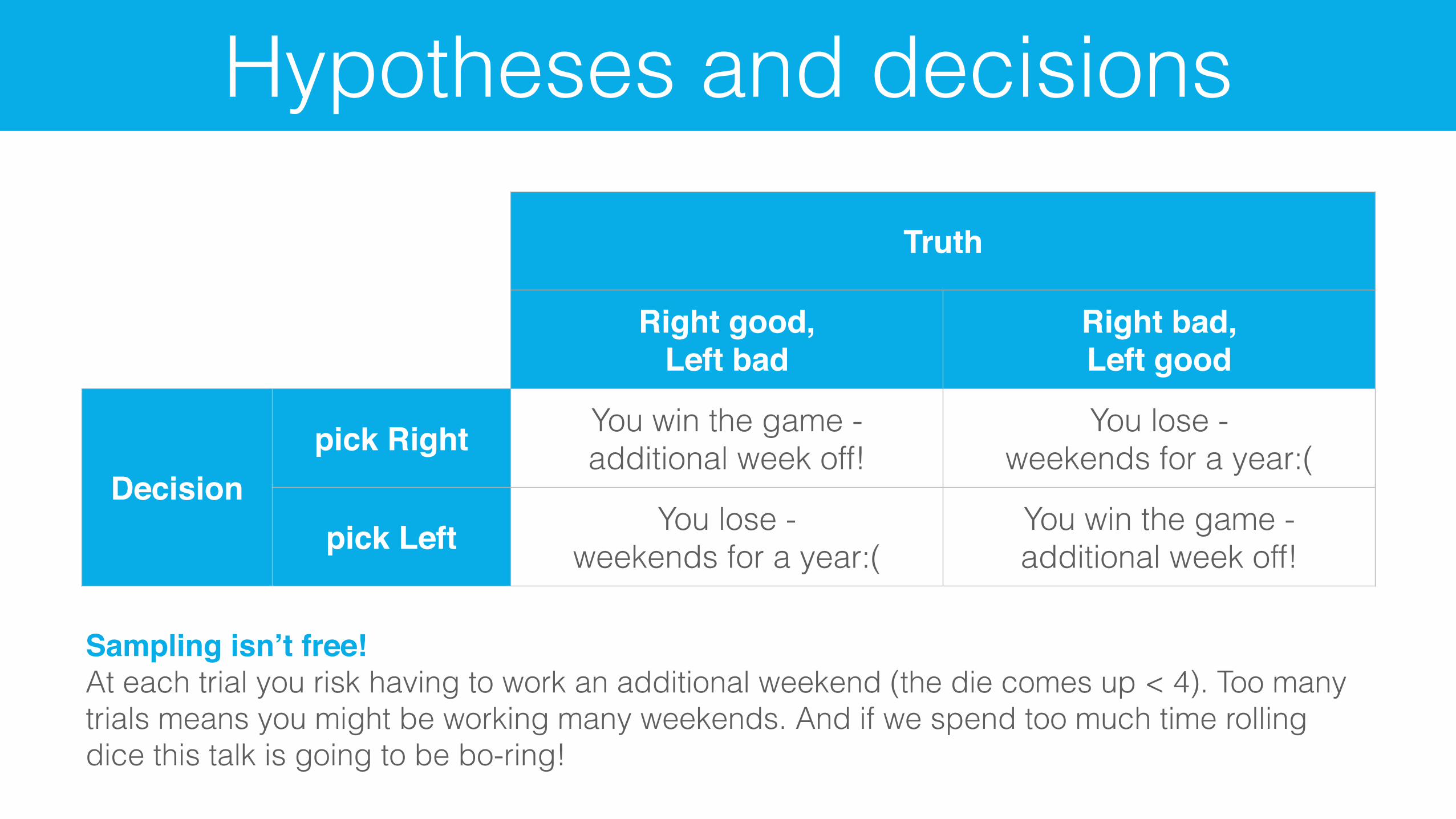
Truth

Right good,Left bad

Right bad,Left good

Decisionpick Right You win the game -

additional week off!You lose -

weekends for a year:(

pick Left You lose - weekends for a year:(

You win the game - additional week off!

Sampling isn’t free!At each trial you risk having to work an additional weekend (the die comes up < 4). Too many trials means you might be working many weekends. And if we spend too much time rolling dice this talk is going to be bo-ring!

Hypotheses and decisions

P(H1) = 0.5 P(H2) = 0.5

Two possible options:

Initial guess

H1: good die on the Right

LEFT RIGHT

H2: bad die on the Right

LEFT RIGHT

Prior probabilities

‣ These are your prior probabilities for the two competing claims:

‣ P(H1: good die on the Right) = 0.5

‣ P(H2: bad die on the Right) = 0.5

‣ These probabilities represent what you believe before seeing any data.

‣ You could have conceivably made up these probabilities, but instead you have chosen to make an educated guess.

Data collection: round 1

≥4

LEFT RIGHT

You chose the right hand, and you won (rolled a number ≥4). Having observed this data point how, if at all, do the probabilities you assign to the same set of hypotheses change?

After you see the data

We can be a little more precise…

P(H1) > 0.5H1: good die on the Right

LEFT RIGHT

P(H2) < 0.5H2: bad die on the Right

LEFT RIGHT

H1: good die on the Right0.5

0.5

H2: bad die on the Right

≥40.75

<40.25

≥40.5

<40.5

0.5 x 0.75 = 0.375

0.5 x 0.25 = 0.125

0.5 x 0.5 = 0.25

0.5 x 0.5 = 0.25

prior likelihood joint

posterior

Posterior probabilities‣ The probabilities we just calculated is called a posterior probabilities:

‣ P(H1: good die on the Right | data) = 0.6

‣ P(H2: bad die on the Right | data) = 0.4

‣ Posterior probabilities are generally defined as P(hypothesis | data).

‣ These probabilities tell us the probability of a hypothesis we set forth, given the data we just observed.

‣ They depend on the prior probabilities as well as the likelihood of the observed data.

‣ Note: This is different than a p-value = P(observed or more extreme outcome | H0 is true).

Bayes’ theorem

posterior ∝ prior × likelihood

Ready to make a call?

Truth

Right good,Left bad

Right bad,Left good

Decisionpick Right You win the game -

additional week off!You lose -

weekends for a year:(

pick Left You lose - weekends for a year:(

You win the game - additional week off!

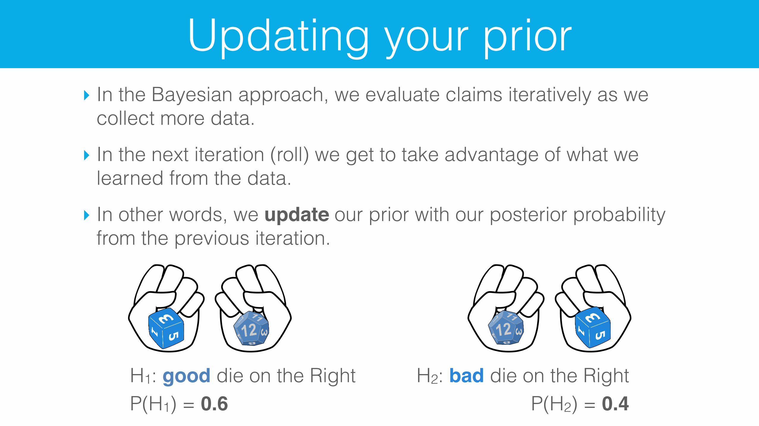
Updating your prior‣ In the Bayesian approach, we evaluate claims iteratively as we

collect more data.

‣ In the next iteration (roll) we get to take advantage of what we learned from the data.

‣ In other words, we update our prior with our posterior probability from the previous iteration.

P(H1) = 0.6H1: good die on the Right H2: bad die on the Right

P(H2) = 0.4

Recap

‣ Take advantage of prior information, like a previously published study or a physical model.

‣ Naturally integrate data as you collect it, and update your priors.

‣ Avoid the counter-intuitive definition of a p-value: P(observed or more extreme outcome | H0 is true)

‣ Instead base decisions on the posterior probability: P(hypothesis is true | observed data).

‣ A good prior helps, a bad prior hurts, but the prior matters less the more data you have.

Practical Bayes

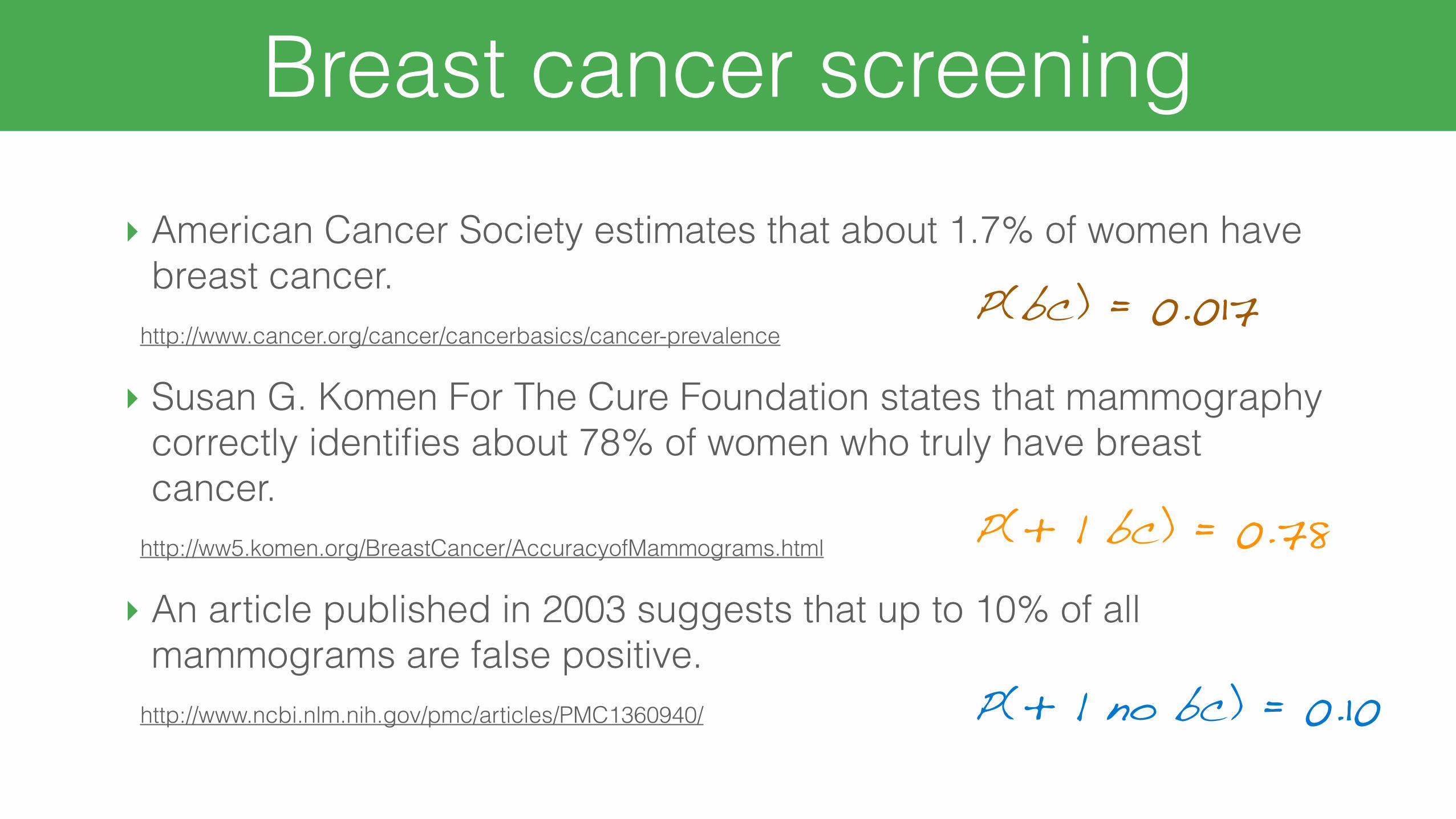
Breast cancer screening‣ American Cancer Society estimates that about 1.7% of women have

breast cancer. http://www.cancer.org/cancer/cancerbasics/cancer-prevalence

‣ Susan G. Komen For The Cure Foundation states that mammography correctly identifies about 78% of women who truly have breast cancer.

http://ww5.komen.org/BreastCancer/AccuracyofMammograms.html

‣ An article published in 2003 suggests that up to 10% of all mammograms are false positive.

http://www.ncbi.nlm.nih.gov/pmc/articles/PMC1360940/

P(bc) = 0.017

P(+ | bc) = 0.78

P(+ | no bc) = 0.10

Prior probabilityPrior to any testing and any information exchange between the patient and the doctor, what probability should a doctor assign to a female patient having breast cancer?

P(bc) = 0.017

Posterior probabilityWhen a patient goes through breast cancer screening there are two competing claims: patient has cancer and patient doesn't have cancer. If a mammogram yields a positive result, what is the probability that patient has cancer?

bc

no bc

0.017P(bc)

0.983P(no bc)

0.78P(+ | bc)

P(- | bc)

+

- 0.22

P(+ | no bc)

P(- | no bc)

+-

0.10

0.90

0.017 x 0.78 = 0.01326P(bc and +)

0.983 x 0.10 = 0.0983P(no bc and +)

P(bc | +) =0.01326

0.01326 + 0.0983≈ 0.12

P(bc and +)P(+)

=

RetestingSince a positive mammogram doesn't necessarily mean that the patient actually has breast cancer, the doctor might decide to re-test the patient. What is the probability of having breast cancer if this second mammogram also yields a positive result?

bc

no bc

0.12P(bc)

0.88P(no bc)

0.78P(+ | bc)

P(- | bc)

+

- 0.22

P(+ | no bc)

P(- | no bc)

+-

0.10

0.90

0.12 x 0.78 = 0.0936P(bc and +)

0.88 x 0.10 = 0.088P(no bc and +)

P(bc | +) =0.0936

0.0936 + 0.088≈ 0.52

P(bc and +)P(+)

Bayesian vs. frequentist inference

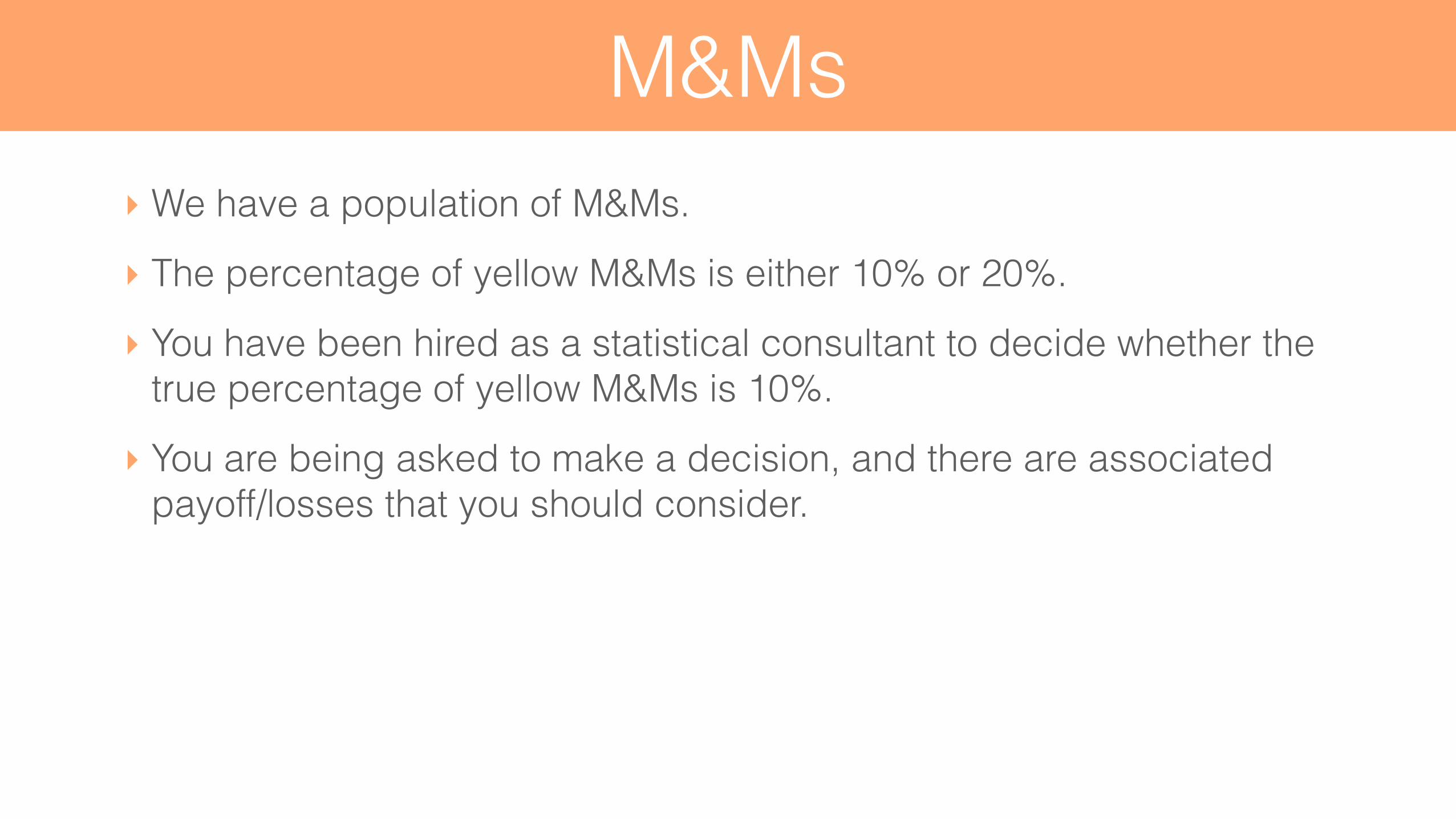
M&Ms‣ We have a population of M&Ms.

‣ The percentage of yellow M&Ms is either 10% or 20%.

‣ You have been hired as a statistical consultant to decide whether the true percentage of yellow M&Ms is 10%.

‣ You are being asked to make a decision, and there are associated payoff/losses that you should consider.

Frequentist inferenceH0: 10% yellow M&MsHA: >10% yellow M&Ms

RGYBO

k = 1, n = 5

→Fail to reject H0

hypotheses

sample

obs. data

p-value

Bayesian inferenceH1: 10% yellow M&MsH2: 20% yellow M&Ms

RGYBOk = 1, n = 5

hypotheses

sample

obs. data

likelihood

posterior

prior

FREQUENTIST BAYESIAN

obs. dataP(k or more | 10% yellow)

P(10% yellow | n,k) P(20% yellow | n,k)

n = 5, k = 1 0.41 0.44 0.56

n = 10, k = 2 0.26 0.39 0.61

n = 15, k = 3 0.18 0.34 0.66

n = 20, k = 4 0.13 0.29 0.71

Bayesian vs. frequentist inference

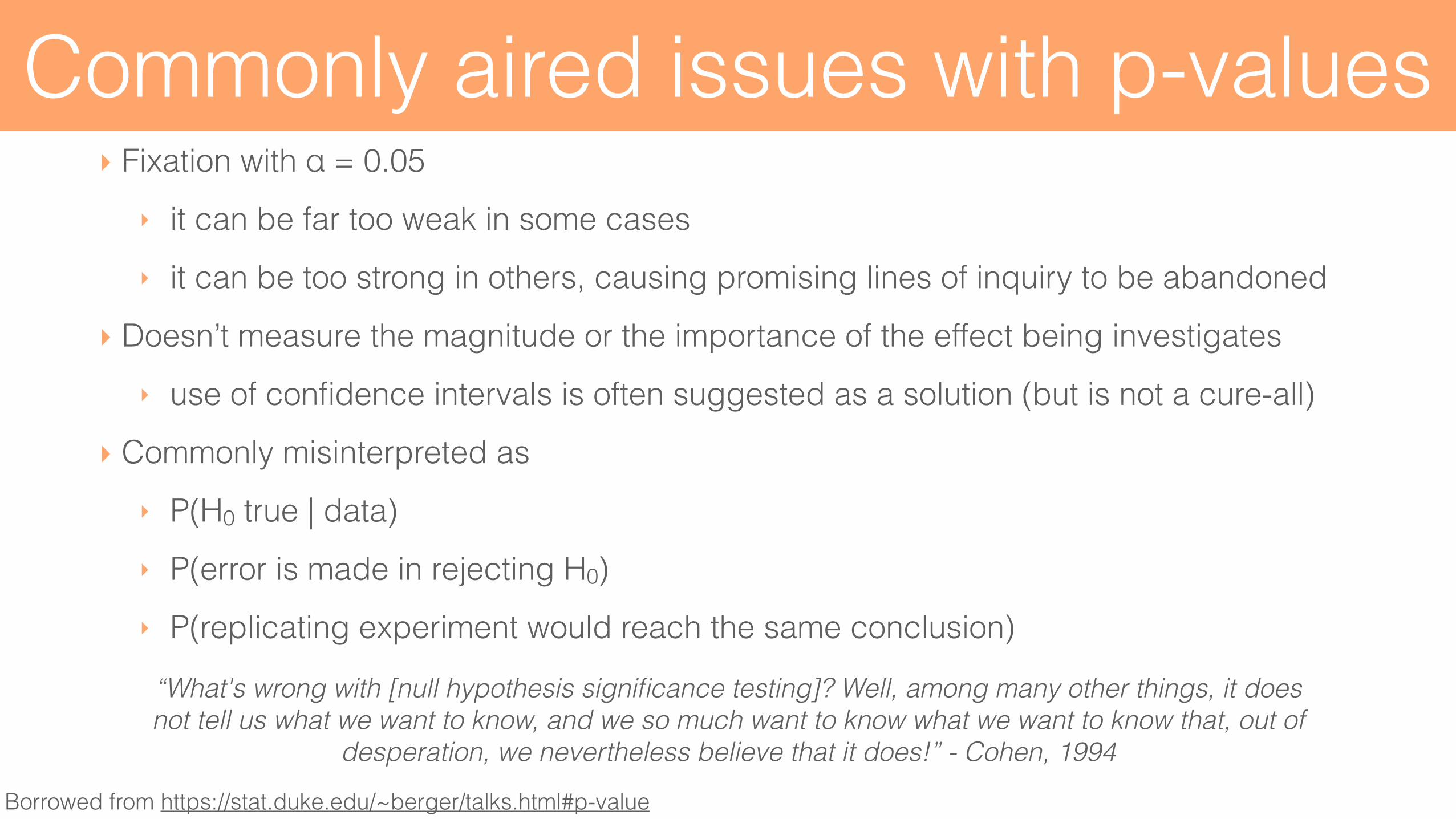
‣ Fixation with α = 0.05 ‣ it can be far too weak in some cases ‣ it can be too strong in others, causing promising lines of inquiry to be abandoned

‣ Doesn’t measure the magnitude or the importance of the effect being investigates ‣ use of confidence intervals is often suggested as a solution (but is not a cure-all)

‣ Commonly misinterpreted as ‣ P(H0 true | data) ‣ P(error is made in rejecting H0) ‣ P(replicating experiment would reach the same conclusion)

Commonly aired issues with p-values

“What's wrong with [null hypothesis significance testing]? Well, among many other things, it does not tell us what we want to know, and we so much want to know what we want to know that, out of

desperation, we nevertheless believe that it does!” - Cohen, 1994

Borrowed from https://stat.duke.edu/~berger/talks.html#p-value

Generalizing Bayes

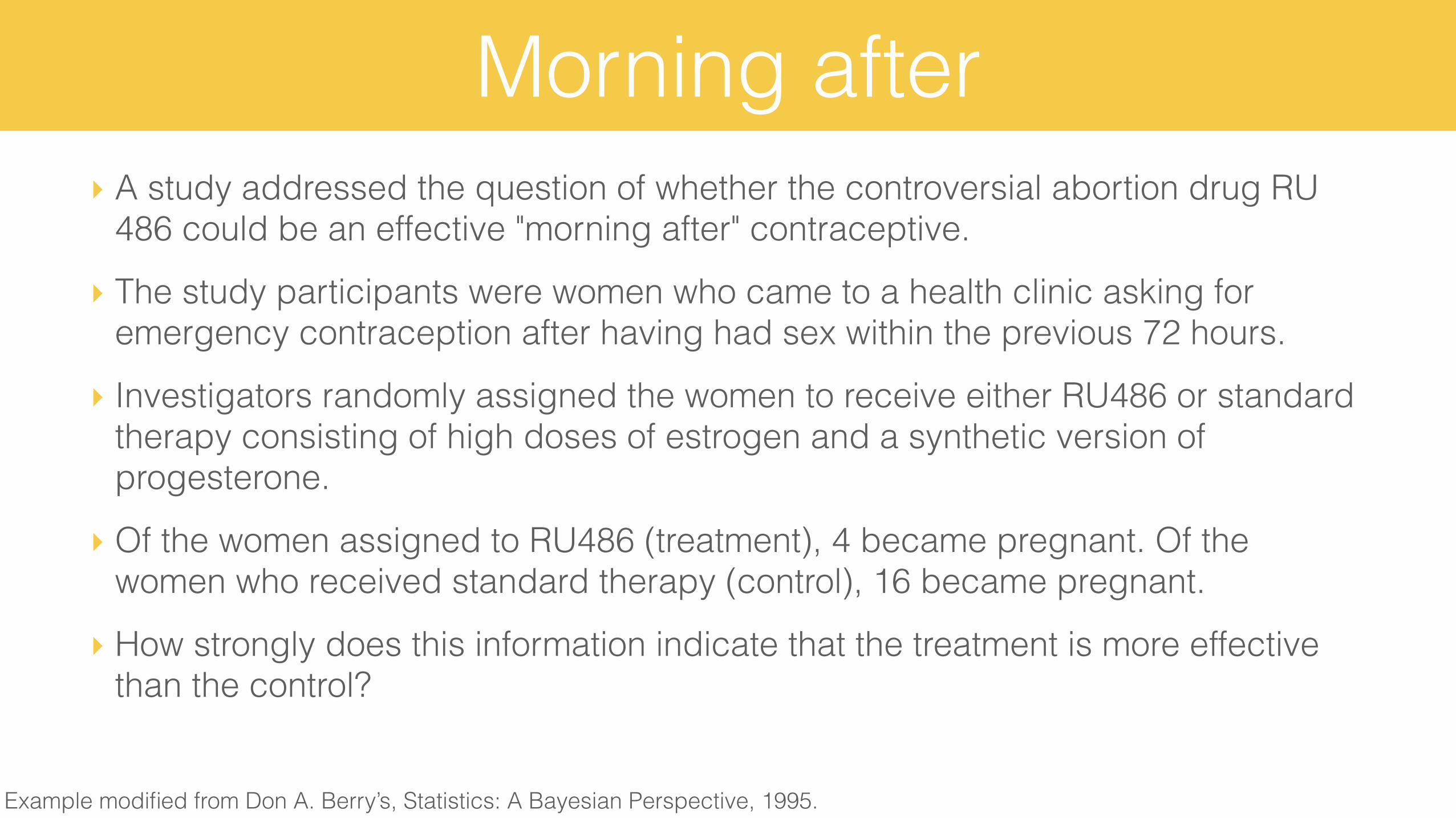
Morning after‣ A study addressed the question of whether the controversial abortion drug RU

486 could be an effective "morning after" contraceptive.

‣ The study participants were women who came to a health clinic asking for emergency contraception after having had sex within the previous 72 hours.

‣ Investigators randomly assigned the women to receive either RU486 or standard therapy consisting of high doses of estrogen and a synthetic version of progesterone.

‣ Of the women assigned to RU486 (treatment), 4 became pregnant. Of the women who received standard therapy (control), 16 became pregnant.

‣ How strongly does this information indicate that the treatment is more effective than the control?

Example modified from Don A. Berry’s, Statistics: A Bayesian Perspective, 1995.

Framework‣ To simplify matters let’s turn this problem of comparing two proportions to a

one proportion problem: consider only the 20 total pregnancies, and ask how likely is it that 4 pregnancies occur in the treatment group.

‣ If the treatment and control are equally effective, and the sample sizes for the two groups are the same, then the probability the pregnancy come from the treatment group is simply p = 0.5.

‣ We’ll consider any value of p between 0 and 1, 0 ≤ p ≤ 1.

Prior distributionAssume an uninformative uniform distribution, where a = 0 and b = 1

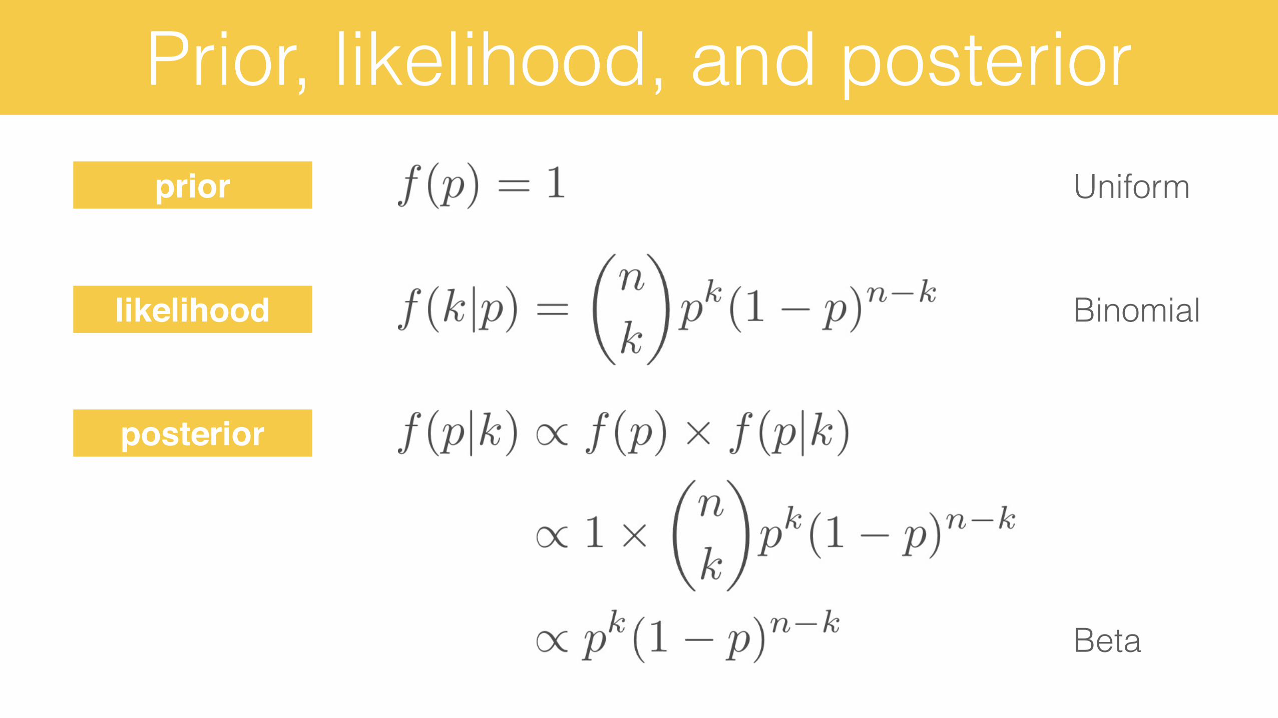
Prior, likelihood, and posteriorprior

likelihood

posterior

Uniform

Binomial

Beta

Prior and posterior, visualizedn = 20, k = 4

What if we had more data?n = 40, k = 8

Or even more data?n = 200, k = 40

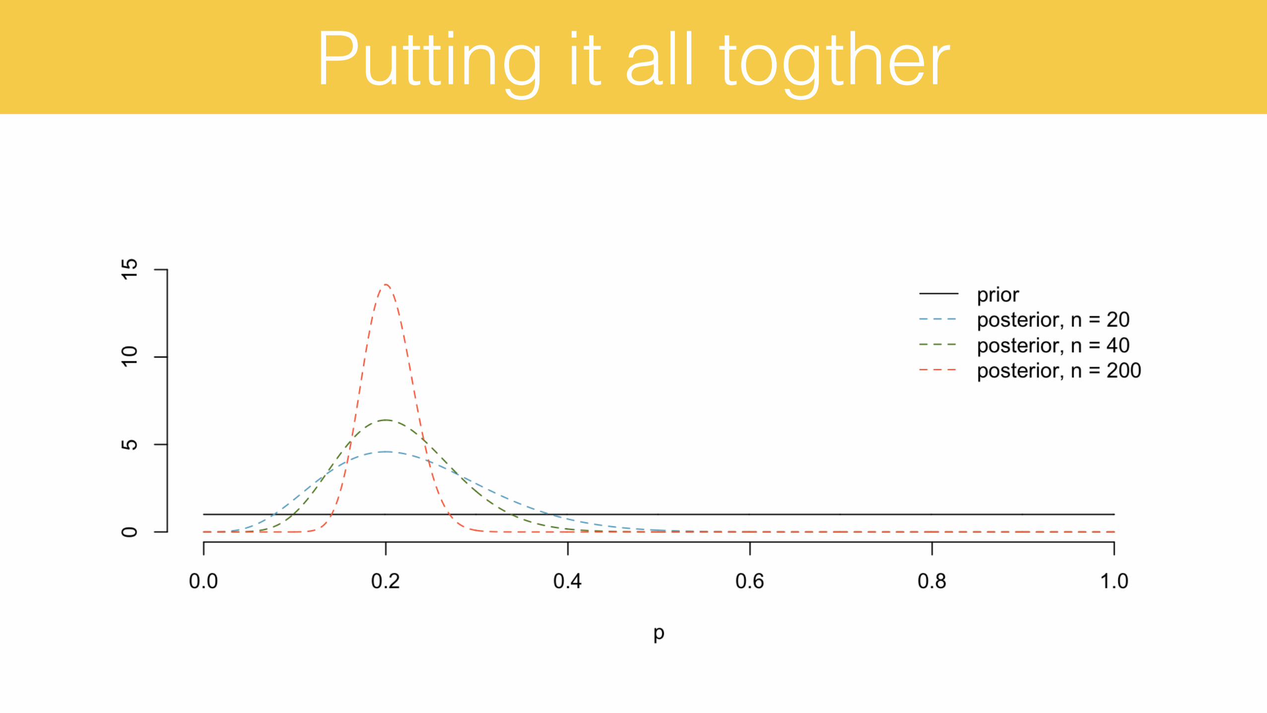
Putting it all togther

Summary

‣ is a natural analog to how we think and learn — updating beliefs based on empirical data

‣ is useful in practical situations

‣ brings basic probability into the context of decision making scenarios more naturally than the frequentist p-value

‣ can be used in the continuous space and when building models

Bayesian thinking…

‣ rely on the choice of the prior, but the prior matters less the more data you have

‣ may require heavier use of computational tools when working with complicated models and/or the posterior does not follow a known distribution

‣ but things can be complicated with frequentist models as well (e.g. there may not be closed form solution for the MLE)

Bayesian approaches…

Thank you!email

slides

mine@stat.duke.edu

http://bit.ly/bayesian_baby_steps