Bayesian Algorithms for Causal Data Miningproceedings.mlr.press/v6/mani10a/mani10a.pdf · Bayesian...

JMLR Workshop and Conference Proceedings 6:121–136 NIPS 2008 workshop on causality

Bayesian Algorithms for Causal Data Mining

Subramani Mani [email protected]

Department of Biomedical InformaticsVanderbilt UniversityNashville, TN, 37232-8340, USA

Constantin F. Aliferis [email protected]

Center for Health Informatics and BioinformaticsNew York UniversityNew York, NY, 10016, USA

Alexander Statnikov [email protected]

Center for Health Informatics and BioinformaticsNew York UniversityNew York, NY, 10016, USA

Editor: Isabelle Guyon, Dominik Janzing and Bernhard Schölkopf

AbstractWe present two Bayesian algorithms CD-B and CD-H for discovering unconfounded cause andeffect relationships from observational data without assuming causal sufficiency which pre-cludes hidden common causes for the observed variables. The CD-B algorithm first estimatesthe Markov blanket of a node X using a Bayesian greedy search method and then applies Baye-sian scoring methods to discriminate the parents and children of X . Using the set of parents andset of children CD-B constructs a global Bayesian network and outputs the causal effects of anode X based on the identification of Y arcs. Recall that if a node X has two parent nodes A,Band a child node C such that there is no arc between A,B and A,B are not parents of C, then thearc from X to C is called a Y arc. The CD-H algorithm uses the MMPC algorithm to estimatethe union of parents and children of a target node X . The subsequent steps are similar to thoseof CD-B. We evaluated the CD-B and CD-H algorithms empirically based on simulated datafrom four different Bayesian networks. We also present comparative results based on the iden-tification of Y structures and Y arcs from the output of the PC, MMHC and FCI algorithms.The results appear promising for mining causal relationships that are unconfounded by hiddenvariables from observational data.

Keywords: Causal data mining, Markov blanket, Y structures

1. Introduction and BackgroundCausal knowledge enables us to plan interventions leading to predictable, measurable and de-sirable outcomes. Experimental data is typically generated for ascertaining cause and effectrelationships. However, experimental studies may not be feasible in many situations due toethical, logistical, cost, technical or other reasons. This study introduces two new Bayesianalgorithms CD-B and CD-H for ascertaining causality from observational data. There are many

c○2010 S. Mani, C. F. Aliferis, and A. Statnikov

MANI ALIFERIS STATNIKOV

algorithms available for learning the underlying causal structure from data such as GS (Mar-garitis and Thrun, 2000), PC (Spirtes et al., 2000, page 84–85), HITON (Aliferis et al., 2003a),OR (Moore and Wong, 2003) and FCI (Spirtes et al., 2000). However, all of these algorithmsexcept FCI make an assumption of causal sufficiency which maintains that there are no unob-served common causes for any two or more of the observed variables. Even though FCI doesnot make such an assumption its usefulness is limited in practical settings due to its scalabilitylimitation.

The Bayesian algorithms proposed in this paper are based on a computationally feasiblescore-based search to identify some causal effects in the large sample limit while allowing forthe possibility of unobserved common causes, and without making any assumptions about thetrue causal structure (other than acyclicity). There is also no need to assign scores explicitly tocausal structures with unobserved common causes in this framework.

We now define some terms that are needed for our causal datamining framework. Ourframework for causal discovery is based on causal Bayesian networks (CBNs). A CBN is aBayesian network in which each arc is interpreted as a direct causal influence between a parentnode (variable) and a child node, relative to the other nodes in the network (Pearl, 1991). We

GFED@ABCW1

��7777GFED@ABCW2

��GFED@ABCW1 GFED@ABCW2

?>=<89:;X

��

GFED@ABCH1

BB��// ?>=<89:;X

��

GFED@ABCH2

\\9999oo

?>=<89:;Z ?>=<89:;Z

G1 G1H

Figure 1: A Y structure G1 and a Y equivalent structure G1H (H1 and H2 denote hidden varia-bles).

proceed to introduce the concept of a Y structure and a Y arc in a Bayesian network. LetW1→ X ←W2 be a V structure (there is no arc between W1 and W2). If there is a node Z suchthat there is an arc from X to Z, but no arc from W1 to Z and no arc from W2 to Z, then the nodesW1,W2,X and Z form a Y structure (see Figure 1, G1). If such a Y structure over four measuredvariables V is learned from an observational dataset D, the arc from X to Z in the Y structurerepresents an unconfounded causal relationship (Mani et al., 2006). Since G1 also has the sameset of independence/dependence relationships over the observed variables (I-map) as G1H (seeFigure 1), the arcs W1→ X and W2→ X in G1 cannot be interpreted as necessarily representingcausal relationships. The arc from X to Z in a Y structure is referred to as a Y arc (YA).

We now define the concept of a Markov blanket which is needed for an understanding ofthe CD-B and CD-H algorithms. The Markov blanket (MB) of a node X in a causal Bayesiannetwork G is the union of the set of parents of X , the children of X , and the parents of thechildren of X .

2. AlgorithmsIn this section we introduce the algorithms in this study for discovering cause and effect rela-tionships from observational data. We first introduce the Bayesian algorithms CD-B and CD-Hthat learn global CBN models and output the set of Y arcs which represent cause and effectrelationships unconfounded by hidden variables. We then provide short descriptions of the

122

CAUSAL DATA MINING

PC, FCI and MMHC algorithms and the post-processing procedure that we use to identify theunconfounded causal arcs from the output of PC and MMHC.

2.1 CD-B algorithm

The CD-B algorithm first induces the Markov blanket (MB) of each node X ∈V (where V is theset of domain variables) using the Bayesian Markov blanket induction (MBI) procedure (Mani,2005). The MBI procedure finds the Markov blanket of a node X under the assumptions ofMarkov, faithfulness and large sample size. It uses a greedy forward and backward search inseeking the Markov blanket of X , which we denote MB(X). The set MB(X) is the estimatedMarkov blanket of X in a data generating network. From the MB of each node X the spousenodes (parents of children of a node X are referred to as the spouse nodes of X) are excludedby a Bayesian dependence heuristic (Cooper, 1997) to obtain the set of parents and children ofX (denoted as PC(X)). Using PC(X) we generate all possible DAGs such that the only arcs arefrom each parent to X and from X to each child. We refer to these DAGs as PC DAGs.

The key insight is that there are exactly 2k such PC DAGs where k = |PC(X)|. The highestscoring DAG from each node set PC(X)∪X is used to get the P(X) and the C(X), that is, theparents and children of X respectively. Using P(X) from the highest scoring PC DAGs withtwo or more parents a global directed graph is constructed. Note that a PC DAG G with P(X)as set of parents and C(X) as set of children of the node X is unique (the only member ofits Markov equivalence class) if |P(X)| ≥ 2. Since all the PC DAGs are scored, this step isexponential in the size of the set of parents and children. To the best of our knowledge thePC DAG method introduced here is the only Bayesian method to partition a set of parents andchildren (P(X)∪C(X)) into the set of parents P(X) and the set of children C(X).

The global directed graph created using the set of parents may contain directed cycles. Adirected cycle is a directed path starting from a node A and ends in node A after traversing twoor more nodes. The cycles in the graph are broken iteratively by removing the “weakest” arcusing a greedy search heuristic till all cycles are eliminated. The C(X) edges from the highestscoring PC DAGs with two or more parents are inserted based on a set of constraints (rules).The union of the edges of the highest scoring PC DAGs with less than two parents are insertedusing a different set of constraints. As already mentioned, when the PC DAG has two or moreparents it is unique, that is, it is the only member of its Markov equivalence class. On the otherhand the PC DAGs with less than two parents are not unique (there is at least one additionalmember in its Markov equivalence class). Hence the arcs belonging to the two categories ofPC DAGs are inserted into the global DAG using different sets of constraints. The resultingDAG is used to identify all the Y arcs. The pseudocode for the CD-B algorithm is provided inAppendix A.1.

2.2 CD-H algorithm

The CD-H algorithm replaces the initial steps of the CD-B algorithm for finding the PC(X) withthe MMPC algorithm (Tsamardinos et al., 2003, 2006). The MMPC uses a two-phase searchprocedure based on tests of independence/dependence. In the first phase of search a candidateset of parents and children called CPC is estimated which is a superset of the parents andchildren (PC) set. The second phase of the search procedure prunes the CPC set yielding the PCset. A proof of correctness and empirical results showing the validity of the MMPC algorithmare provided in (Tsamardinos et al., 2003). The subsequent steps of the CD-H algorithm aresimilar to CD-B.

123


2.3 PC algorithm

The PC algorithm takes as input a dataset D over a set of observed random variables V, a condi-tional independence test, and an α level of significance threshold for a test of statistical indepen-dence and then outputs an essential graph. PC also makes an assumption of causal sufficiency.This means that all the variables of the causal network are measured and there is no attempt todiscover latent (hidden) variables. Hence PC is not designed to discover hidden variables thatare common causes of any pair of observed variables. In the worst case, PC is exponential inthe largest degree (size of the set of parents and children of a node) in the data generating DAG.See (Spirtes et al., 2000, page 84–85) for more details on the PC algorithm. The PC algorithmoutputs both directed and undirected edges. A post-processing step (procedure YA) that we addis performed on the set of arcs to identify the Y structures. The pseudocode for procedure YAis given in Appendix A.1.3.

2.4 FCI algorithm

The FCI algorithm takes as input a dataset D over a set of random variables V and outputs agraphical model consisting of edges between variables that have a cause and effect interpreta-tion. While the PC algorithm outputs only directed and undirected edges, the FCI algorithmoutputs a richer set of edges to denote the presence of hidden (unmeasured) confounding va-riables and various levels of uncertainty in the orientation of the edges (Spirtes et al., 2000).The FCI algorithm can handle hidden variables and sample selection bias that are likely to bepresent in real-world datasets. It is possible to obtain causal relationships that are unconfoundedby hidden variables from the partial ancestral graph (PAG) output of the FCI algorithm. Theedges oriented as A→ B in the FCI output can be interpreted as an unconfounded causal arcsimilar to a Y arc.

2.5 MMHC algorithm

The max-min hill-climbing (MMHC) Bayesian network structure learning algorithm is a hybridalgorithm that combines ideas from constraint-based and score-based methods (Tsamardinoset al., 2006). MMHC has been extensively evaluated on a variety of structure learning tasksfrom different datasets and outperformed PC, FCI, the Sparse Candidate, Optimal Reinsertionand the Greedy Equivalence Search algorithms. The MMHC algorithm estimates the set ofparents and children of a node X denoted by PC(X) using the MMPC algorithm (Tsamardinoset al., 2003) to first obtain an undirected skeleton of the output graph. MMHC then uses greedysteepest-ascent TABU search and the Bayesian scoring measure BDeu (Heckerman et al., 1995)to orient the edges.

3. Experimental methodsIn this section we describe the experimental methods used to evaluate our causal discovery ap-proach. We used expert-defined CBNs to (1) generate data from those models, (2) apply thecausal discovery algorithm to the data, and (3) evaluate the causal relationships output by thealgorithm relative to the data generating CBNs that serve as gold standards. The output of the al-gorithm was compared with the data generating structure and scored as explained below. CD-Band CD-H algorithms were implemented in Matlab. The PC and FCI algorithms implemented inTetrad IV (http://www.phil.cmu.edu/projects/tetrad) were used. The MMHCimplementation in the Causal Explorer package (Aliferis et al., 2003b) was used. For PC,MMHC, CD-B and CD-H algorithms the Y arcs output by the algorithms were compared with

124

CAUSAL DATA MINING

the Y arcs of the data generating networks and for FCI the fully oriented arcs were used. Recallthat a post-processing step was required for PC and MMHC algorithms to obtain the Y arcs.Precision, recall and F-measure were computed for the algorithms as follows:

Precision: (# of Y arcs correctly identified) / (# of total Y arcs output).

Recall: (# of Y arcs correctly identified) / (# of total Y arcs present in the datagenerating network).

F measure: (2 * recall * precision) / (recall + precision).

Four Bayesian networks built by domain experts in such varied fields as medicine, atmosphericsciences and agriculture were identified. These networks are Alarm (Beinlich et al., 1990),Hailfinder (Abramson et al., 1996), Barley (Kristensen and Rasmussen, 2002), and Munin (An-dreassen et al., 1987). For causal discovery, we generated simulated training instances bystochastic sampling (Henrion, 1986). Varying sample sizes in the range of 1,000 to 20,000instances were used in our causal discovery experiments. Table 1 gives the distribution of thenodes, arcs and Y structures for the various networks used in our study. Typically default pa-

Table 1: Nodes, arcs and Y structures in the Alarm, Hailfinder, Barley, and Munin networks

Category Alarm Hailfinder Barley Munin

Nodes 37 56 48 189Arcs 46 66 84 282Y structures 13 20 44 147

rameters were used to run the algorithms with some adjustments made for uniformity. ThePC algorithm was run with default parameters (significance level 0.05). CD-B was also runwith default parameters (maximum MB size 12, dependency threshold for spouse elimination0.9). CD-H was run with the following parameters: maximum size of conditioning set 10 andsignificance threshold 0.05. All the algorithms were run on each of the sample sizes usingthe ACCRE (Linux) cluster in Vanderbilt University consisting of x86 processors with 3.8 GBmemory. Each job was assigned to a single processor with a time limit of 48 hours.

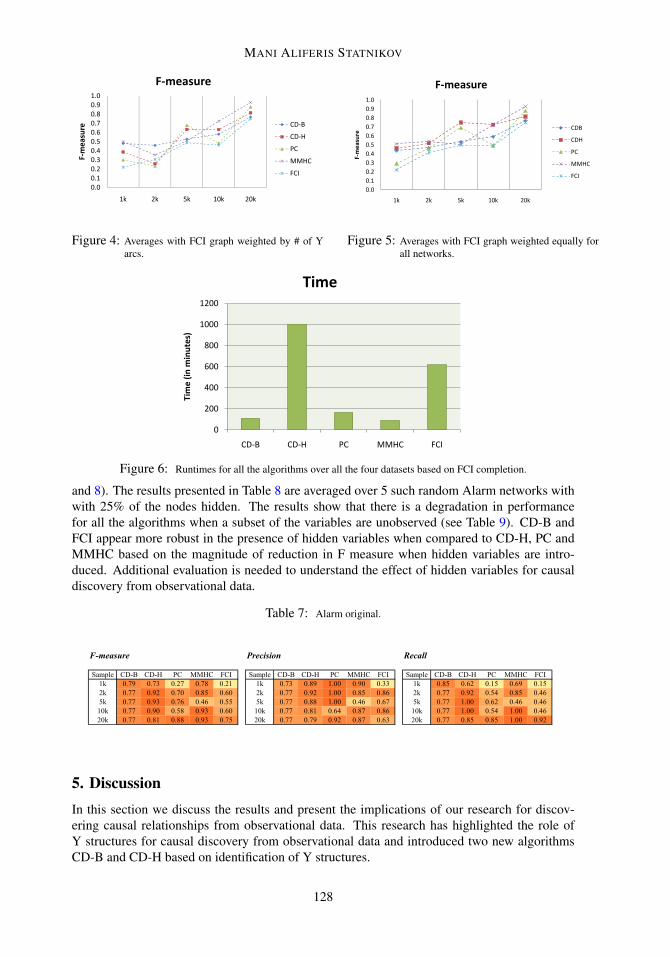
4. ResultsThe results presented below are based on sample sizes of 1K, 2K, 5K, 10K and 20K instancesfor each of the four domain datasets that were generated. We present a summary performanceof all the four algorithms based on Y arcs present in all the data generating networks usingprecision, recall and F-measure as explained below. The aggregate results are presented basedon the following two methods.

(i). The various data generating networks are given equal weight in the analysis irrespectiveof the number of Y arcs.

(ii). The data generating networks are weighted by the number of Y arcs present in eachnetwork.

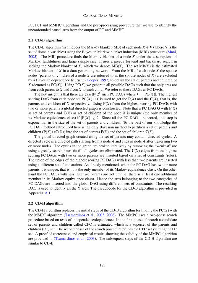
Altogether there were 224 YA in the four domain CBNs. The results presented are based onaverages over all the four networks unless specified otherwise (see Tables 2, 3 and Figures 2, 3).The highest precision of 0.97 (equal weight) and 0.95 (weighted by # of Y arcs) were achieved at

125


Table 2: Averages without FCI table weighted by # of Y arcs.

Weighted by the number of Y-arcs

F-measure Precision Recall

Sample CD-B CD-H PC MMHC Sample CD-B CD-H PC MMHC Sample CD-B CD-H PC MMHC

1k 0.34 0.27 0.15 0.32 1k 0.79 0.28 0.90 0.43 1k 0.21 0.27 0.08 0.25

2k 0.41 0.30 0.22 0.33 2k 0.84 0.31 0.93 0.40 2k 0.27 0.29 0.13 0.29

5k 0.47 0.34 0.29 0.34 5k 0.82 0.31 0.95 0.40 5k 0.33 0.38 0.17 0.29

10k 0.47 0.38 0.30 0.52 10k 0.83 0.39 0.79 0.57 10k 0.33 0.38 0.18 0.48

20k 0.52 0.44 0.34 0.44 20k 0.81 0.39 0.65 0.45 20k 0.38 0.50 0.23 0.44

Weighted equally



1k 0.32 0.41 0.20 0.40 1k 0.76 0.44 0.93 0.61 1k 0.29 0.39 0.14 0.32

2k 0.39 0.50 0.35 0.46 2k 0.78 0.52 0.93 0.59 2k 0.32 0.49 0.26 0.40

5k 0.49 0.51 0.45 0.38 5k 0.76 0.51 0.97 0.51 5k 0.39 0.57 0.36 0.32

10k 0.48 0.52 0.38 0.60 10k 0.76 0.54 0.78 0.69 10k 0.39 0.55 0.33 0.56

20k 0.54 0.55 0.45 0.58 20k 0.80 0.59 0.73 0.60 20k 0.44 0.57 0.43 0.58

Table 3: Averages without FCI table weighted equally.




1k 0.34 0.27 0.15 0.32 1k 0.79 0.28 0.90 0.43 1k 0.21 0.27 0.08 0.25

2k 0.41 0.30 0.22 0.33 2k 0.84 0.31 0.93 0.40 2k 0.27 0.29 0.13 0.29

5k 0.47 0.34 0.29 0.34 5k 0.82 0.31 0.95 0.40 5k 0.33 0.38 0.17 0.29

10k 0.47 0.38 0.30 0.52 10k 0.83 0.39 0.79 0.57 10k 0.33 0.38 0.18 0.48

20k 0.52 0.44 0.34 0.44 20k 0.81 0.39 0.65 0.45 20k 0.38 0.50 0.23 0.44

Weighted equally



1k 0.32 0.41 0.20 0.40 1k 0.76 0.44 0.93 0.61 1k 0.29 0.39 0.14 0.32

2k 0.39 0.50 0.35 0.46 2k 0.78 0.52 0.93 0.59 2k 0.32 0.49 0.26 0.40

5k 0.49 0.51 0.45 0.38 5k 0.76 0.51 0.97 0.51 5k 0.39 0.57 0.36 0.32

10k 0.48 0.52 0.38 0.60 10k 0.76 0.54 0.78 0.69 10k 0.39 0.55 0.33 0.56

20k 0.54 0.55 0.45 0.58 20k 0.80 0.59 0.73 0.60 20k 0.44 0.57 0.43 0.58

0

0.1

0.2

0.3

0.4

0.5

0.6

0.7

0.8

0.9

1

1k 2k 5k 10k 20k

F-measure

F-measure

CDB

CDH

PC

MMHC

0

0.1

0.2

0.3

0.4

0.5

0.6

0.7

0.8

0.9

1

1k 2k 5k 10k 20k

F-measure

F-measure

CDB

CDH

PC

MMHC

Figure 2: Averages without FCI graph weighted by # ofY arcs.

0

0.1

0.2

0.3

0.4

0.5

0.6

0.7

0.8

0.9

1

1k 2k 5k 10k 20k

F-measure

F-measure

CDB

CDH

PC

MMHC

0

0.1

0.2

0.3

0.4

0.5

0.6

0.7

0.8

0.9

1

1k 2k 5k 10k 20k

F-measure

F-measure

CDB

CDH

PC

MMHC

Figure 3: Averages without FCI graph weighted equallyfor all networks.

126

CAUSAL DATA MINING

the sample size of 5,000 with PC. In general PC and CD-B had higher precision (≥ 0.65) acrossall the sample sizes tested. The best recall was obtained by MMHC (0.58 equally weighted)and CD-H (0.50 when weighted by # of Y arcs) with a sample size of 20,000. The best F-measure (when equally weighted) of 0.60 was achieved by MMHC (sample size 10K) followedby 0.55 for CD-H (sample size 20K). The best F-measure (weighted by # of Y arcs) of 0.52 wasachieved by MMHC (sample size 10K) and CD-B (sample size 20K).

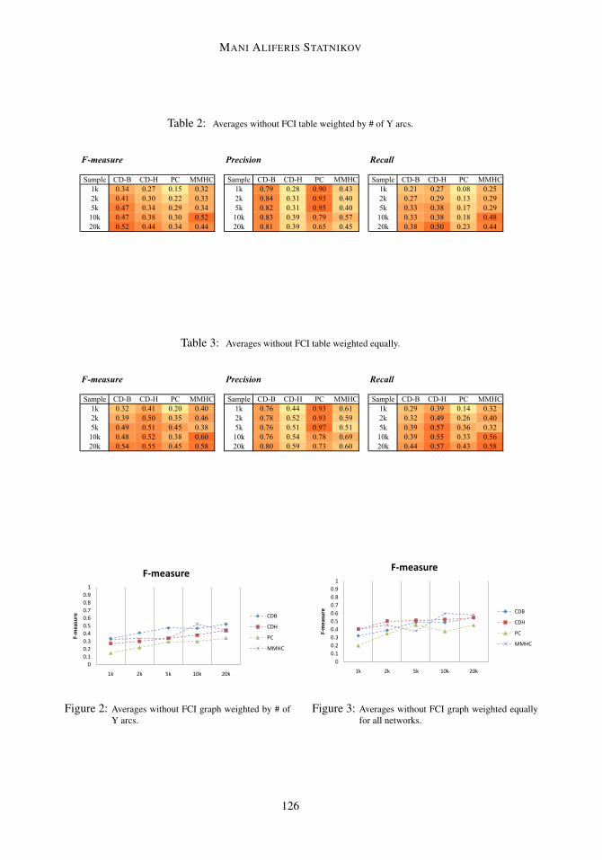
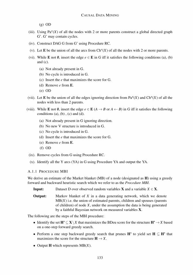
FCI could be run without going out of memory or exceeding the time limit of 48 hourson all sample sizes only for the Alarm dataset. Out of 20 experiments (5 sample sizes x 4datasets), FCI ran out of memory in 9 cases (for all sample sizes in Barley network and forsample sizes 1K, 5K, 10K, and 20K in Munin network), ran out of time in 1 case (sample size20K for Hailfinder network), and completed with results in the remaining 10 experiments (seeTables 4, 5 and Figures 4, 5). Based on F measure FCI performance is generally lower whencompared with the other algorithms across all the sample sizes. Figure 6 shows total run time forall algorithms for the latter 10 experiments. As can be seen, FCI is the second slowest algorithmafter CD-H. However, CD-H was able to complete with results in all 20 experiments, thus it ismore useful for practitioners despite being one of the slowest algorithms in the comparison.CD-H runs slow primarily because it includes false positives in the estimated PC sets whichmakes PC DAG search much more computationally expensive. Table 6 provides the runtimesof the various algorithms for the Alarm dataset. FCI runtime is an order of magnitude highercompared to the other algorithms on the Alarm dataset.

Table 4: Averages with FCI table weighted by # of Y arcs.

2k 0.46 0.26 0.23 0.35 0.31 2k 0.84 0.27 0.92 0.39 0.79 2k 0.32 0.25 0.13 0.32 0.19

F‐measure Precision Recall

Sample CD‐B CD‐H PC MMHC FCI Sample CD‐B CD‐H PC MMHC FCI Sample CD‐B CD‐H PC MMHC FCI1k 0.48 0.39 0.30 0.50 0.22 1k 0.71 0.41 0.86 0.80 0.42 1k 0.36 0.36 0.18 0.36 0.152k 0.46 0.26 0.23 0.35 0.31 2k 0.84 0.27 0.92 0.39 0.79 2k 0.32 0.25 0.13 0.32 0.195k 0.53 0.63 0.68 0.51 0.49 5k 0.70 0.53 1.00 0.64 0.65 5k 0.42 0.79 0.52 0.42 0.3910k 0.58 0.63 0.48 0.72 0.46 10k 0.73 0.56 0.62 0.84 0.57 10k 0.48 0.73 0.39 0.64 0.3920k 0.77 0.81 0.88 0.93 0.75 20k 0.77 0.79 0.92 0.87 0.63 20k 0.77 0.85 0.85 1.00 0.92

Table 5: Averages with FCI table weighted equally.



Sample CD-B CD-H PC MMHC FCI Sample CD-B CD-H PC MMHC FCI Sample CD-B CD-H PC MMHC FCI

1k 0.54 0.51 0.30 0.50 0.04 1k 0.62 0.54 0.86 0.80 0.42 1k 0.48 0.48 0.18 0.36 0.02

2k 0.43 0.53 0.23 0.35 0.25 2k 0.67 0.54 0.92 0.39 0.79 2k 0.32 0.52 0.13 0.32 0.15

5k 0.51 0.74 0.68 0.51 0.11 5k 0.60 0.65 1.00 0.64 0.65 5k 0.45 0.85 0.52 0.42 0.06

10k 0.64 0.75 0.48 0.72 0.11 10k 0.78 0.67 0.62 0.84 0.57 10k 0.55 0.85 0.39 0.64 0.06

20k 0.79 0.81 0.88 0.93 0.10 20k 0.79 0.76 0.92 0.87 0.63 20k 0.79 0.86 0.85 1.00 0.05

Weighted equally



1k 0.44 0.46 0.29 0.51 0.22 1k 0.62 0.54 0.90 0.75 0.42 1k 0.45 0.41 0.18 0.42 0.15

2k 0.47 0.52 0.46 0.54 0.42 2k 0.77 0.52 0.90 0.62 0.77 2k 0.39 0.51 0.32 0.49 0.32

5k 0.53 0.75 0.69 0.51 0.50 5k 0.67 0.66 1.00 0.68 0.65 5k 0.48 0.88 0.53 0.43 0.41

10k 0.59 0.72 0.49 0.73 0.49 10k 0.72 0.65 0.62 0.83 0.65 10k 0.53 0.83 0.42 0.70 0.41

20k 0.77 0.81 0.88 0.93 0.75 20k 0.77 0.79 0.92 0.87 0.63 20k 0.77 0.85 0.85 1.00 0.92

Table 6: Alarm original network runtimes in minutes for all the algorithms.

Sample CD-B CD-H PC MMHC FCI

1k 0.20 0.30 0.10 0.10 5.00

2k 0.30 0.30 0.10 0.10 1.00

5k 0.50 0.50 0.10 0.20 5.00

10k 0.70 0.70 0.10 0.20 5.00

20k 1.10 0.90 0.20 0.40 58.00

0

10

20

30

40

50

60

70

1k 2k 5k 10k 20k

Tim

e in

min

ute

s

Time

CD-B

CD-H

PC

MMHC

FCI

We also present results of causal discovery in the presence of hidden variables based onrandomly assigning “hidden” status to 25% of the variables for the Alarm dataset (see Tables 7

127


0.00.10.20.30.40.50.60.70.80.91.0

1k 2k 5k 10k 20k

F‐measure

F‐measure

CD‐B

CD‐H

PC

MMHC

FCI

Figure 4: Averages with FCI graph weighted by # of Yarcs.

0

0.1

0.2

0.3

0.4

0.5

0.6

0.7

0.8

0.9

1

1k 2k 5k 10k 20k

F-measure

F-measure

CDB

CDH

PC

MMHC

FCI

0.0

0.1

0.2

0.3

0.4

0.5

0.6

0.7

0.8

0.9

1.0

1k 2k 5k 10k 20k

F-measure

F-measure

CDB

CDH

PC

MMHC

FCI

Figure 5: Averages with FCI graph weighted equally forall networks.

ALARM


1k 0.20 0.30 0.10 0.10 5.00

2k 0.30 0.30 0.10 0.10 1.00

5k 0.50 0.50 0.10 0.20 5.00

10k 0.70 0.70 0.10 0.20 5.00

20k 1.10 0.90 0.20 0.40 58.00

BARLEY


1k - - - - M

2k - - - - M

5k - - - - M

10k - - - - M

20k - - - - M

HAILFINDER


1k 6.00 26.00 0.20 0.60 6.00

2k 8.30 36.00 4.60 1.10 61.00

5k 22.50 92.50 31.40 4.00 150.00

10k 57.50 222.50 126.10 12.10 261.00

20k - - - - T

MUNIN


1k - - - - M

2k 12.80 622.90 2.60 70.80 66.00

5k - - - - M

10k - - - - M

20k - - - - M

0

100

200

300

400

500

600

700

1k 2k 5k 10k 20k

Tim

e in

min

ute

s

Time

CD-B

CD-H

PC

MMHC

FCI

0

200

400

600

800

1000

1200

CD-B CD-H PC MMHC FCI

Tim

e (

in m

inu

tes)

Time

Figure 6: Runtimes for all the algorithms over all the four datasets based on FCI completion.

and 8). The results presented in Table 8 are averaged over 5 such random Alarm networks withwith 25% of the nodes hidden. The results show that there is a degradation in performancefor all the algorithms when a subset of the variables are unobserved (see Table 9). CD-B andFCI appear more robust in the presence of hidden variables when compared to CD-H, PC andMMHC based on the magnitude of reduction in F measure when hidden variables are intro-duced. Additional evaluation is needed to understand the effect of hidden variables for causaldiscovery from observational data.

Table 7: Alarm original.



1k 0.79 0.73 0.27 0.78 0.21 1k 0.73 0.89 1.00 0.90 0.33 1k 0.85 0.62 0.15 0.69 0.15

2k 0.77 0.92 0.70 0.85 0.60 2k 0.77 0.92 1.00 0.85 0.86 2k 0.77 0.92 0.54 0.85 0.46

5k 0.77 0.93 0.76 0.46 0.55 5k 0.77 0.88 1.00 0.46 0.67 5k 0.77 1.00 0.62 0.46 0.46

10k 0.77 0.90 0.58 0.93 0.60 10k 0.77 0.81 0.64 0.87 0.86 10k 0.77 1.00 0.54 1.00 0.46

20k 0.77 0.81 0.88 0.93 0.75 20k 0.77 0.79 0.92 0.87 0.63 20k 0.77 0.85 0.85 1.00 0.92



1k 0.60 0.38 0.22 0.49 0.19 1k 0.75 0.53 0.70 0.75 0.28 1k 0.52 0.31 0.13 0.38 0.15

2k 0.60 0.50 0.32 0.43 0.40 2k 0.73 0.57 0.80 0.52 0.41 2k 0.52 0.46 0.21 0.38 0.39

5k 0.51 0.65 0.49 0.27 0.43 5k 0.67 0.65 1.00 0.38 0.51 5k 0.42 0.67 0.35 0.22 0.38

10k 0.57 0.54 0.54 0.47 0.58 10k 0.64 0.58 0.69 0.53 0.51 10k 0.52 0.52 0.45 0.44 0.67

20k 0.58 0.61 0.56 0.57 0.66 20k 0.65 0.60 0.80 0.66 0.58 20k 0.54 0.62 0.47 0.54 0.79

5. DiscussionIn this section we discuss the results and present the implications of our research for discov-ering causal relationships from observational data. This research has highlighted the role ofY structures for causal discovery from observational data and introduced two new algorithmsCD-B and CD-H based on identification of Y structures.

128

CAUSAL DATA MINING

Table 8: Alarm 75 percent observed.



1k 0.79 0.73 0.27 0.78 0.21 1k 0.73 0.89 1.00 0.90 0.33 1k 0.85 0.62 0.15 0.69 0.15

2k 0.77 0.92 0.70 0.85 0.60 2k 0.77 0.92 1.00 0.85 0.86 2k 0.77 0.92 0.54 0.85 0.46

5k 0.77 0.93 0.76 0.46 0.55 5k 0.77 0.88 1.00 0.46 0.67 5k 0.77 1.00 0.62 0.46 0.46

10k 0.77 0.90 0.58 0.93 0.60 10k 0.77 0.81 0.64 0.87 0.86 10k 0.77 1.00 0.54 1.00 0.46

20k 0.77 0.81 0.88 0.93 0.75 20k 0.77 0.79 0.92 0.87 0.63 20k 0.77 0.85 0.85 1.00 0.92



1k 0.60 0.38 0.22 0.49 0.19 1k 0.75 0.53 0.70 0.75 0.28 1k 0.52 0.31 0.13 0.38 0.15

2k 0.60 0.50 0.32 0.43 0.40 2k 0.73 0.57 0.80 0.52 0.41 2k 0.52 0.46 0.21 0.38 0.39

5k 0.51 0.65 0.49 0.27 0.43 5k 0.67 0.65 1.00 0.38 0.51 5k 0.42 0.67 0.35 0.22 0.38

10k 0.57 0.54 0.54 0.47 0.58 10k 0.64 0.58 0.69 0.53 0.51 10k 0.52 0.52 0.45 0.44 0.67

20k 0.58 0.61 0.56 0.57 0.66 20k 0.65 0.60 0.80 0.66 0.58 20k 0.54 0.62 0.47 0.54 0.79

Table 9: Alarm 75 performance degradation.

Original



1k 0.79 0.73 0.27 0.78 0.21 1k 0.73 0.89 1.00 0.90 0.33 1k 0.85 0.62 0.15 0.69 0.15

2k 0.77 0.92 0.70 0.85 0.60 2k 0.77 0.92 1.00 0.85 0.86 2k 0.77 0.92 0.54 0.85 0.46

5k 0.77 0.93 0.76 0.46 0.55 5k 0.77 0.88 1.00 0.46 0.67 5k 0.77 1.00 0.62 0.46 0.46

10k 0.77 0.90 0.58 0.93 0.60 10k 0.77 0.81 0.64 0.87 0.86 10k 0.77 1.00 0.54 1.00 0.46

20k 0.77 0.81 0.88 0.93 0.75 20k 0.77 0.79 0.92 0.87 0.63 20k 0.77 0.85 0.85 1.00 0.92

75%



1k 0.60 0.38 0.22 0.49 0.19 1k 0.75 0.53 0.70 0.75 0.28 1k 0.52 0.31 0.13 0.38 0.15

2k 0.60 0.50 0.32 0.43 0.40 2k 0.73 0.57 0.80 0.52 0.41 2k 0.52 0.46 0.21 0.38 0.39

5k 0.51 0.65 0.49 0.27 0.43 5k 0.67 0.65 1.00 0.38 0.51 5k 0.42 0.67 0.35 0.22 0.38

10k 0.57 0.54 0.54 0.47 0.58 10k 0.64 0.58 0.69 0.53 0.51 10k 0.52 0.52 0.45 0.44 0.67

20k 0.58 0.61 0.56 0.57 0.66 20k 0.65 0.60 0.80 0.66 0.58 20k 0.54 0.62 0.47 0.54 0.79

F-measure


1k -0.18 -0.35 -0.04 -0.30 -0.02

2k -0.17 -0.43 -0.38 -0.42 -0.20

5k -0.26 -0.28 -0.27 -0.19 -0.11

10k -0.20 -0.36 -0.05 -0.45 -0.02

20k -0.18 -0.21 -0.32 -0.36 -0.09

Precision varied within a narrow range of 0.76 to 0.84 for CD-B and between 0.65 and 0.97for PC (see Tables 2 and 3). The relatively narrow precision range for the different samplesizes combined with a monotonic increase in recall throughout the sample range shows thatthe performance of CD-B and PC is robust across a wide range of sample sizes. In generalprecision values are higher compared to recall values for all the sample sizes except for theCD-H algorithm. Note that a higher precision translates to lower number of false positives eventhough some causal relationships may not be reported. A desirable goal in causal discovery isto keep the proportion of false positives low even if it entails a trade-off in terms of recall.

FCI and CD-H had longer runtimes when compared with PC, MMHC and CD-B. It is possi-ble to use symmetry correction in the MMPC step of the CD-H algorithm to reduce the numberof false positives in the PC set and decrease runtime.

The causal discovery framework that we presented for identifying direct causal relationshipsis dependent on the presence of Y structures in the data generating process. The two medical(Alarm, Munin) and two non-medical (Hailfinder, Barley) networks that were used to generatedata had varying numbers of Y structures. These networks were created by domain expertscapturing the probabilistic dependencies and independencies in the domain. Hence it seemsplausible that Y structures occur in the data generating process of many real-world domains.Presence of Y structures have also been shown in a real world infant birth and death dataset(Mani and Cooper, 2004).

CD-B and CD-H are unique in differentiating the set of parents and the set of children of anode X from the union of the set of parents and children of X . Identification of the parents andchildren of a node will give us the candidate set of direct causes and the candidate set of directeffects of a node. Due to the presence of hidden variables all the parents cannot be interpreted asdirect causes and all the children cannot be interpreted as direct effects. However, the candidateset of parents and children can be used to rule out hypothesized causes or effects. Also, whenexperimental studies are feasible the candidate sets can act as the first filter and provide theexperimenter with a preliminary set of potential causes and effects. Moreover, the set of parentsor the set of children of a node completely specify a directed acyclic graph which can be usedto approximate the data generating model.

129


5.1 Related work

The most related algorithm to the CD-B algorithm is the BLCD (Mani and Cooper, 2004; Mani,2005). BLCD estimates the Markov blanket of a variable and uses it for the identification of Ystructures from sets of four variables. BLCD does not specifically identify the sets of parentsand children from the Markov blanket.

Aliferis et al. have introduced HITON, an algorithm to determine the MB of an outcomevariable (Aliferis et al., 2003a). Tsamardinos et al. have described an algorithm called MMMBand they discuss that since the MB contains direct causes and direct effects of a variable X , theMB has causal interpretability (Tsamardinos et al., 2003). Note that both HITON and MMMBdo not specifically distinguish between causes and effects of a node; however, they do output thevariables that have direct edges during the operation of the algorithm. Additional processing (orexperimentation) of HITON and MMMB output is required to determine causal directionality.

5.2 Limitations and future work

There are two main types of limitations of this work. The first set of limitations results from theframework and assumptions we have chosen for causal discovery. The second set of limitationsis due to the specifics of the algorithm and the experimental methods that were used.

The CBN framework imposes a directed acyclic graph structure on all causal phenomena.Discovering causal mechanisms that incorporate feedback cycles can be problematic unlesstime is represented explicitly and cycles are “unfolded” to provide a DAG structure (Cooper,1999). The causal discovery approach we have taken is not complete in the sense that we candiscover only causal relationships represented in nature as Y structures. The algorithms alsocurrently requires that the modeled variables be discrete.

The evaluation measures of precision, recall and F measure that were used are structural.Hence the evaluation of the purported causal relationships were structural, leaving out the para-metric components. That is, we evaluated how well the algorithm can discover the presenceof a causal influence, but leave to future work the characterization of how well the algorithmcaptures the functional relationships among the causes and effects.

We plan to apply the CD-B and CD-H algorithms to real-world datasets as part of our futurework.

Acknowledgments

We thank professor Greg Cooper for helpful discussions. We thank Yerbolat Dosbayev forimplementing CD-B and CD-H and Yukun Chen for running the experiments and generatingthe results presented in the paper. We also thank the anonymous reviewers for their criticalcomments and suggestions for improving the paper.

ReferencesBruce Abramson, John Brown, Ward Edwards, Allan Murphy, and Robert L. Winkler. Hail-

finder: A Bayesian System for Forecasting Severe Weather. International Journal of Fore-casting, 12:57–71, 1996.

Constantin F. Aliferis, Ioannis Tsamardinos, and Alexander Stanikov. HITON, A novel markovblanket algorithm for optimal variable selection. In Proceedings of the AMIA Fall Symposium,2003a.

130

CAUSAL DATA MINING

Constantin F. Aliferis, Ioannis Tsamardinos, Alexander Stanikov, and Laura E. Brown. CausalExplorer: A causal probabilistic network learning toolkit for biomedical discovery. In Pro-ceedings of the 2003 International Conference on Mathematics and Engineering Techniquesin Medicine and Biological Sciences (METMBS), 2003b.

Steen Andreassen, Marianne Woldbye, Bjorn Falck, and Stig K. Andersen. MUNIN — A causalprobabilistic network for interpretation of electromyographic findings. In Proceedings of theTenth International Joint Conference on Artificial Intelligence, pages 366–372, San Mateo,CA, 1987. Morgan Kaufmann.

Ingo A. Beinlich, H.J. Suermondt, R. Martin Chavez, and Gregory F. Cooper. The ALARMmonitoring system: A case study with two probabilistic inference techniques for belief net-works. In Proceedings of the Second European Conference on Artificial Intelligence inMedicine, pages 247–256, London, 1990. Chapman and Hall.

Gregory F. Cooper. A simple constraint-based algorithm for efficiently mining observationaldatabases for causal relationships. Data Mining and Knowledge Discovery, 1:203–224, 1997.

Gregory F. Cooper. An Overview of the Representation and Discovery of Causal RelationshipsUsing Bayesian Networks. In Clark Glymour and Gregory F. Cooper, editors, Computation,Causation, and Discovery, pages 3–62. MIT Press, Cambridge, MA, 1999.

David Heckerman, Dan Geiger, and David M. Chickering. Learning Bayesian networks: Thecombination of knowledge and statistical data. Machine Learning, 20(3):197–243, 1995.

Max Henrion. Propagating uncertainty in bayesian networks by probabilistic logic sampling. InProceedings of the 2nd Annual Conference on Uncertainty in Artificial Intelligence (UAI-86),New York, NY, 1986. Elsevier Science Publishing Company, Inc.

K. Kristensen and I.A. Rasmussen. The use of a Bayesian network in the design of a deci-sion support system for growing malting barley without use of pesticides. Computers andElectronics in Agriculture, 33:197–217, 2002.

Subramani Mani. A Bayesian Local Causal Discovery Framework. PhD thesis, University ofPittsburgh, 2005.

Subramani Mani and Gregory F. Cooper. Causal discovery using a Bayesian local causal dis-covery algorithm. In M. Fieschi et al. editor, Proceedings of MedInfo, pages 731–735. IOSPress, 2004.

Subramani Mani, Peter Spirtes, and Gregory F. Cooper. A theoretical study of Y structures forcausal discovery. In Rina Dechter and Thomas S. Richardson, editors, Proceedings of theConference on Uncertainty in Artificial Intelligence, pages 314–323, Corvallis, OR, 2006.AUAI Press.

Dimitris Margaritis and Sebastian Thrun. Bayesian network induction via local neighborhoods.In S.A.Solla, T.K.Leen, and K.R.Muller, editors, Advances in neural information processingsystems, volume 12, pages 505–511, Cambridge, MA, 2000. MIT Press.

Andrew Moore and Weng-Keen Wong. Optimal reinsertion: A new search operator for accel-erated and more accurate bayesian network structure learning. In T. Fawcett and N. Mishra,editors, Proceedings of the 20th International Conference on Machine Learning (ICML ’03),pages 552–559, Menlo Park, California, August 2003. AAAI Press.

131


Judea Pearl. Probabilistic Reasoning in Intelligent Systems. Morgan Kaufmann, San Francisco,California, 2nd edition, 1991.

Peter Spirtes, Clark Glymour, and Richard Scheines. Causation, Prediction, and Search. MITPress, Cambridge, MA, 2nd edition, 2000.

Ioannis Tsamardinos, Constantin F. Aliferis, and Alexander Stanikov. Time and sample efficientdiscovery of markov blankets and direct causal relations. In Proceedings of the 9th CANSIGKDD International Conference on Knowledge Discovery and Data Mining, pages 673–678, 2003.

Ioannis Tsamardinos, Laura Brown, and Constantin Aliferis. The max-min hill-climbing Baye-sian network structure learning algorithm. Machine Learning, 65:31–78, 2006.

Appendix A. CD-B PseudocodeIn this section we provide the pseudocode for the CD-B algorithm and the details of the variousprocedures called by CD-B, specifically the Markov blanket induction (MBI) procedure and theY arc (YA) finding procedure.

A.1 CD-B algorithm

/* Note: When the PC DAG has 0 or 1 parent Gmax is not unique. We pick any Gmax PC DAGfrom its equivalence class. This implies that in the data generating DAG the edges of such PCDAGs can have either A→ B or A← B orientation. */

Input : Dataset D and the set of variables X.

Output : Pairwise causal influences of the form A→ B representing Y arcs.

The following are the steps of the algorithm:

(i). For each variable X ∈X estimate MB(X) using the Bayesian MB induction (MBI) proce-dure.

(ii). For each variable X ∈ X DO

(a) Update MB(X). If A is in the MB of B, but B is not in the MB of A, we add B to theMB of A.

(b) Remove the spouse nodes from MB(X) to obtain PC(X). Any node independent ofX is excluded from MB(X). Let B denote PC(X).

(c) From B∪X generate all possible DAGs such that the only arcs are from each parentto X and from X to each child. Let this set of DAGs be G.

(d) From the set of DAGs G identify the maximally scoring DAG G using the BDeuscoring measure (Heckerman et al., 1995). Let this DAG be Gmax. If there is a tiefor Gmax, it is broken randomly.

(e) If the Gmax has 2 or more parents mark the Pa(X) and Ch(X) as oriented (Pao(X)and Cho(X)).

(f) If the Gmax has less than 2 parents mark the Pa(X) and Ch(X) as unoriented (Pau(X)and Chu(X)).

132

CAUSAL DATA MINING

(g) OD

(iii). Using Pao(X) of all the nodes with 2 or more parents construct a global directed graphG’. G’ may contain cycles.

(iv). Construct DAG G from G’ using Procedure RC.

(v). Let E be the union of all the arcs from Cho(X) of all the nodes with 2 or more parents.

(vi). While E not /0, insert the edge e ∈ E in G iff it satisfies the following conditions (a), (b)and (c).

(a) Not already present in G.(b) No cycle is introduced in G.(c) Insert the e that maximizes the score for G.(d) Remove e from E.(e) OD

(vii). Let E be the union of all the edges ignoring direction from Pau(X) and Chu(X) of all thenodes with less than 2 parents.

(viii). While E not /0, insert the edge e ∈ E (A→ B or A← B) in G iff it satisfies the followingconditions (a), (b) , (c) and (d).

(a) Not already present in G ignoring direction.(b) No new V structure is introduced in G.(c) No cycle is introduced in G.(d) Insert the e that maximizes the score for G.(e) Remove e from E.(f) OD

(ix). Remove cycles from G using Procedure RC.

(x). Identify all the Y arcs (YA) in G using Procedure YA and output the YA.

A.1.1 PROCEDURE MBI

We derive an estimate of the Market blanket (MB) of a node (designated as H) using a greedyforward and backward heuristic search which we refer to as the Procedure MBI.

Input: Dataset D over observed random variables X and a variable X ∈ X.

Output: Markov blanket of X in a data generating network, which we denoteMB(X) i.e. the union of estimated parents, children and spouses (parentsof children) of node X , under the assumption the data is being generatedby a faithful Bayesian network on measured variables X.

The following are the steps of the MBI procedure:

∙ Identify the set H’⊆X∖X that maximizes the BDeu score for the structure H’→X basedon a one-step forward greedy search.

∙ Perform a one step backward greedy search that prunes H’ to yield set H ⊆ H’ thatmaximizes the score for the structure H→ X .

∙ Output H which represents MB(X).

133


A.1.2 PROCEDURE RC

This procedure removes the cycles from a directed graph. The “weakest” arc is removed itera-tively till all cycles are eliminated.

Input: A directed graph G’.

Output: A directed acyclic graph G.

The following are the steps of the procedure:

(i). Check for cycle(s) in G’. If no cycle assign G’ to G and return G.

(ii). Identify all the arcs forming cycle(s). Let these set of arcs be E.

(iii). Identify the weakest arc E ∈ E by iteratively removing each arc from E and scoring thegraph using the BDeu scoring measure. The arc causing the least reduction in the BDeuscore is determined to be the weakest.

(iv). Remove E from G’. Let the resulting graph be G’. GOTO Step 1.

A.1.3 PROCEDURE YA

We identify all the unique Y arcs (YA) in a DAG G using this procedure. The procedure looksfor all the embedded Y structures (EYS) in G. We say that G contains an embedded Y structureinvolving the variables W1,W2,X and Z, iff all and only the following adjacencies hold amongthe variables W1,W2,X and Z (A2B means that there is no arc between A and B):∙ W12W2; W12Z; W22Z

∙ W1→ X ; W2→ X ; X → Z

Input: A DAG G and a set of nodes X in G.

Output: A set of Y arcs denoted as Y.

Initialize set of YA as Y := {}.For each X ∈ XDO

Determine Pa(X) for X .If |Pa(X)| ≤ 1

Continue /* Next iteration */Determine Ch(X) for X .If |Ch(X)|< 1

Continue /* Next iteration */

/* Look for Y structure */For each pair of parents W1,W2 of XDO

If W1 and W2 are adjacent then ContinueFor each child Z ∈ Ch(X)DO

If (W1,Z) or (W2,Z) adjacent then ContinueIf (X → Z) /∈ Y

134

CAUSAL DATA MINING

Y := Y ∪{X → Z}OD

ODODReturn Y

135


136

Bayesian Algorithms for Causal Data Miningproceedings.mlr.press/v6/mani10a/mani10a.pdf · Bayesian...

Documents

Transcript of Bayesian Algorithms for Causal Data Miningproceedings.mlr.press/v6/mani10a/mani10a.pdf · Bayesian...