Bayes Networks - University of...
69
slide 1 Bayes Networks Xiaojin Zhu [email protected] Computer Sciences Department University of Wisconsin, Madison [based on Andrew Moore’s slides]
Transcript of Bayes Networks - University of...

slide 1
Bayes Networks
Xiaojin Zhu
Computer Sciences Department
University of Wisconsin, Madison
[based on Andrew Moore’s slides]

slide 2
Outline
• Joint probability is great for inference in a uncertain world, but is terrible to obtain and store
• Bayes net allows us to build joint distributions in manageable chunks
Independence, conditional independence
• Bayes net can do any inference
but naïve algorithms can be terribly inefficient
Some inference algorithms can be more efficient
• Parameter learning in Bayes nets

slide 3
Joint distribution
• Making a joint distribution of N variables:
1. List all combinations of values (if each var has k
values, kN combinations)
2. Assign each combination a probability number
3. They should sum to 1
Weather Temperature Prob.
Sunny Hot 150/365
Sunny Cold 50/365
Cloudy Hot 40/365
Cloudy Cold 60/365
Rainy Hot 5/365
Rainy Cold 60/365
slide 4
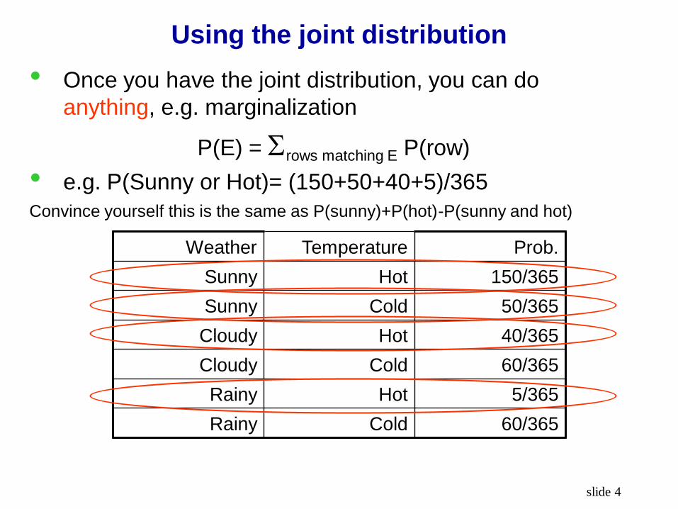
Using the joint distribution
• Once you have the joint distribution, you can do
anything, e.g. marginalization
P(E) = rows matching E P(row)
• e.g. P(Sunny or Hot)= (150+50+40+5)/365
Convince yourself this is the same as P(sunny)+P(hot)-P(sunny and hot)
Weather Temperature Prob.
Sunny Hot 150/365
Sunny Cold 50/365
Cloudy Hot 40/365
Cloudy Cold 60/365
Rainy Hot 5/365
Rainy Cold 60/365

slide 5
Using the joint distribution
• You can also do inference
rows matching Q AND E P(row)
P(Q|E) =
rows matching E P(row)
Weather Temperature Prob.
Sunny Hot 150/365
Sunny Cold 50/365
Cloudy Hot 40/365
Cloudy Cold 60/365
Rainy Hot 5/365
Rainy Cold 60/365
P(Hot | Rainy)

slide 6
The Bad News
• Joint distribution can take up huge space
• For N variables, each taking k values, the joint
distribution has kN numbers
• It would be good to use fewer numbers…

slide 7
Using fewer numbers
• Suppose there are two events:
B: there’s burglary in your house
E: there’s an earthquake
• The joint distribution of them has 4 entries
• Do we have to invent these 4 numbers, for each
combination P(B, E), P(B, ~E), P(~B,E), P(~B,~E)?
Can we ‘derive’ them using P(B) and P(E)?
What assumption do we need?
slide 8
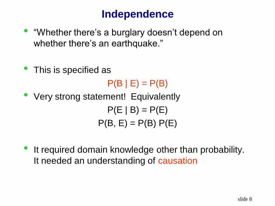
Independence
• “Whether there’s a burglary doesn’t depend on
whether there’s an earthquake.”
• This is specified as
P(B | E) = P(B)
• Very strong statement! Equivalently
P(E | B) = P(E)
P(B, E) = P(B) P(E)
• It required domain knowledge other than probability.
It needed an understanding of causation
slide 9
Independence
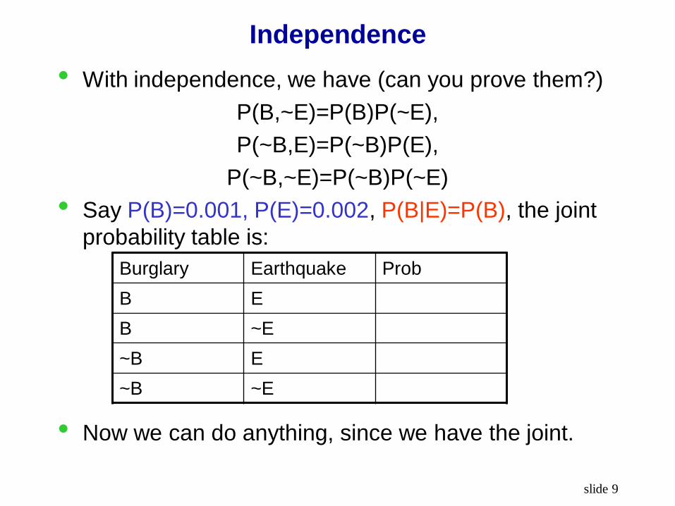
• With independence, we have (can you prove them?)
P(B,~E)=P(B)P(~E),
P(~B,E)=P(~B)P(E),
P(~B,~E)=P(~B)P(~E)
• Say P(B)=0.001, P(E)=0.002, P(B|E)=P(B), the joint
probability table is:
• Now we can do anything, since we have the joint.
Burglary Earthquake Prob
B E
B ~E
~B E
~B ~E

slide 10
A more interesting example
B: there’s burglary in your house
E: there’s an earthquake
A: your alarm sounds
• Your alarm is supposed to sound when there’s a
burglary. But it sometimes doesn’t. And it can
occasionally be triggered by an earthquake
slide 11
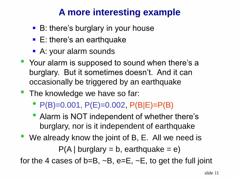
A more interesting example
B: there’s burglary in your house
E: there’s an earthquake
A: your alarm sounds
• Your alarm is supposed to sound when there’s a
burglary. But it sometimes doesn’t. And it can
occasionally be triggered by an earthquake
• The knowledge we have so far:
• P(B)=0.001, P(E)=0.002, P(B|E)=P(B)
• Alarm is NOT independent of whether there’s
burglary, nor is it independent of earthquake
• We already know the joint of B, E. All we need is
P(A | burglary = b, earthquake = e)
for the 4 cases of b=B, ~B, e=E, ~E, to get the full joint

slide 12
A more interesting example
B: there’s burglary in your house
E: there’s an earthquake
A: your alarm sounds
• Your alarm is supposed to sound when there’s a
burglary. But it sometimes doesn’t. And it can
occasionally be triggered by an earthquake
• These 6 numbers specify the joint, instead of 7
• Savings are larger with more variables!
P(B)=0.001
P(E)=0.002
P(B|E)=P(B)
P(A | B, E)=0.95
P(A | B, ~E)=0.94
P(A | ~B, E)=0.29
P(A | ~B, ~E)=0.001

slide 13
A more interesting example
B: there’s burglary in your house
E: there’s an earthquake
A: your alarm sounds
• Your alarm is supposed to sound when there’s a
burglary. But it sometimes doesn’t. And it can
occasionally be triggered by an earthquake
• These 6 numbers specify the joint, instead of 7
• Savings are larger with more variables!
P(B)=0.001
P(E)=0.002
P(B|E)=P(B)
P(A | B, E)=0.95
P(A | B, ~E)=0.94
P(A | ~B, E)=0.29
P(A | ~B, ~E)=0.001
slide 14
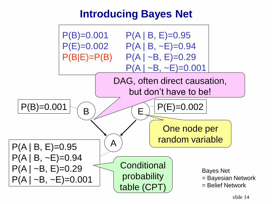
Introducing Bayes Net
P(B)=0.001
P(E)=0.002
P(B|E)=P(B)
P(A | B, E)=0.95
P(A | B, ~E)=0.94
P(A | ~B, E)=0.29
P(A | ~B, ~E)=0.001
B E
A
P(B)=0.001 P(E)=0.002
P(A | B, E)=0.95
P(A | B, ~E)=0.94
P(A | ~B, E)=0.29
P(A | ~B, ~E)=0.001
One node per
random variable
Conditional
probability
table (CPT)
Bayes Net
= Bayesian Network
= Belief Network
DAG, often direct causation,
but don’t have to be!

slide 15
Join probability with Bayes Net
B E
A
P(B)=0.001 P(E)=0.002
P(A | B, E)=0.95
P(A | B, ~E)=0.94
P(A | ~B, E)=0.29
P(A | ~B, ~E)=0.001
One node per
random variable
Conditional
probability
table (CPT)
P(x1,…xN) = i P(xi | parents(xi))
• Example: P(~B, E, ~A) = P(~B) P(E) P(~A | ~B, E)
DAG, often direct causation,
but don’t have to be!

slide 16
Join probability with Bayes Net
B E
A
P(B)=0.001 P(E)=0.002
P(A | B, E)=0.95
P(A | B, ~E)=0.94
P(A | ~B, E)=0.29
P(A | ~B, ~E)=0.001
One node per
random variable
Conditional
probability
table (CPT)
DAG, often direct causation,
but don’t have to be!
P(x1,…xN) = i P(xi | parents(xi))
• Example: P(~B, E, ~A) = P(~B) P(E) P(~A | ~B, E)
• Recall the chain rule:
P(~B, E, ~A) = P(~B) P(E | ~B) P(~A | ~B, E)
Our B.N. has this
independence
assumption

slide 17
More to the story…
A: your alarm sounds
J: your neighbor John calls you
M: your other neighbor Mary calls you
John and Mary do not communicate (they promised
to call you whenever they hear the alarm)
• What kind of independence do we have?
• What does the Bayes Net look like?

slide 18
More to the story…
A: your alarm sounds
J: your neighbor John calls you
M: your other neighbor Mary calls you
John and Mary do not communicate (they promised
to call you whenever they hear the alarm)
• What kind of independence do we have?
• Conditional independence P(J,M|A)=P(J|A)P(M|A)
• What does the Bayes Net look like?
A
J M
slide 19
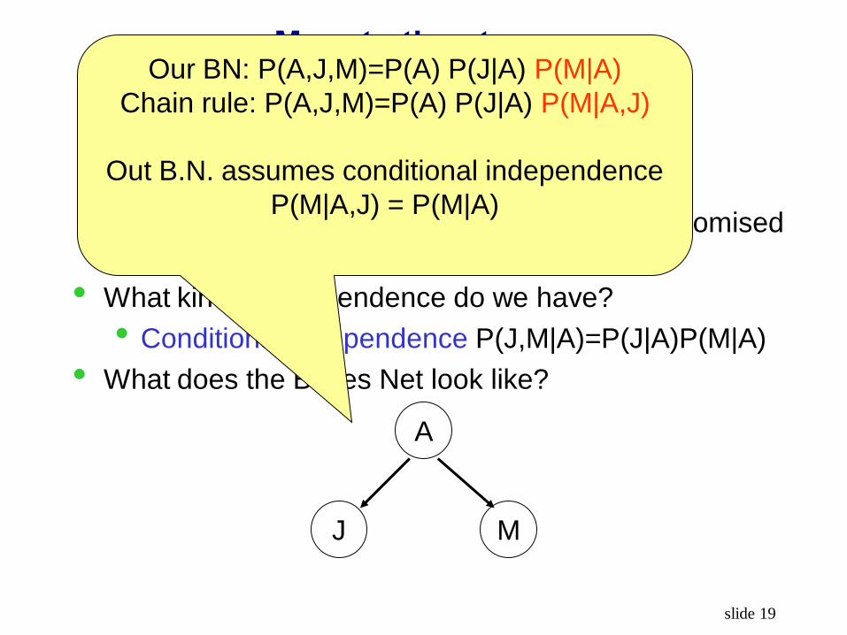
More to the story…
A: your alarm sounds
J: your neighbor John calls you
M: your other neighbor Mary calls you
John and Mary do not communicate (they promised
to call you whenever they hear the alarm)
• What kind of independence do we have?
• Conditional independence P(J,M|A)=P(J|A)P(M|A)
• What does the Bayes Net look like?
A
J M
Our BN: P(A,J,M)=P(A) P(J|A) P(M|A)
Chain rule: P(A,J,M)=P(A) P(J|A) P(M|A,J)
Out B.N. assumes conditional independence
P(M|A,J) = P(M|A)

slide 20
Now with 5 variables
B: there’s burglary in your house
E: there’s an earthquake
A: your alarm sounds
J: your neighbor John calls you
M: your other neighbor Mary calls you
• B, E are independent
• J is only directly influenced by A (i.e. J is conditionally
independent of B, E, M, given A)
• M is only directly influenced by A (i.e. M is
conditionally independent of B, E, J, given A)

slide 21
Creating a Bayes Net
• Step 1: add variables. Choose the variables you
want to include in the Bayes Net
B: there’s burglary in your house
E: there’s an earthquake
A: your alarm sounds
J: your neighbor John calls you
M: your other neighbor Mary calls you
B E
A
J M

slide 22
Creating a Bayes Net
• Step 2: add directed edges.
• The graph must be acyclic.
• If node X is given parents Q1, …, Qm, you are
promising that any variable that’s not a
descendent of X is conditionally independent of X
given Q1, …, Qm
B: there’s burglary in your house
E: there’s an earthquake
A: your alarm sounds
J: your neighbor John calls you
M: your other neighbor Mary calls you
B E
A
J M
slide 23
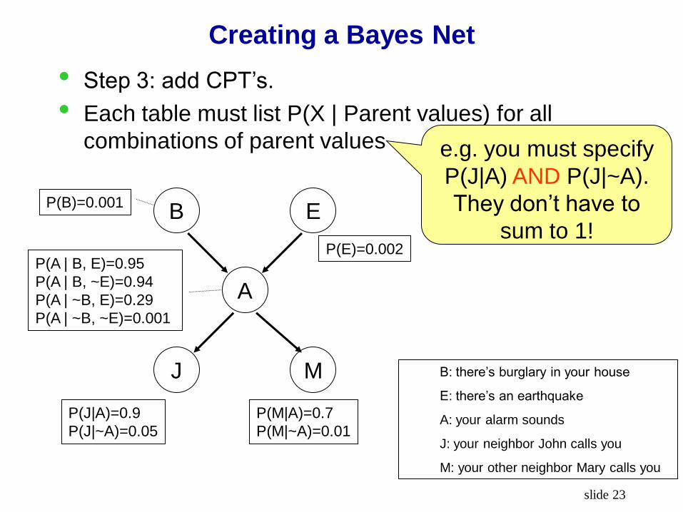
Creating a Bayes Net
• Step 3: add CPT’s.
• Each table must list P(X | Parent values) for all
combinations of parent values
B: there’s burglary in your house
E: there’s an earthquake
A: your alarm sounds
J: your neighbor John calls you
M: your other neighbor Mary calls you
B E
A
J M
e.g. you must specify
P(J|A) AND P(J|~A).
They don’t have to
sum to 1!
P(B)=0.001
P(A | B, E)=0.95
P(A | B, ~E)=0.94
P(A | ~B, E)=0.29
P(A | ~B, ~E)=0.001
P(E)=0.002
P(J|A)=0.9
P(J|~A)=0.05
P(M|A)=0.7
P(M|~A)=0.01

slide 24
Creating a Bayes Net
1. Choose a set of relevant variables
2. Choose an ordering of them, call them x1, …, xN
3. for i = 1 to N:
1. Add node xi to the graph
2. Set parents(xi) to be the minimal subset of
{x1…xi-1}, such that xi is conditionally
independent of all other members of {x1…xi-1}
given parents(xi)
3. Define the CPT’s for
P(xi | assignments of parents(xi))

slide 25
Conditional independence
• Case 1: tail-to-tail
• a, b in general not independent
• But a, b conditionally independent given c
• c is a ‘tail-to-tail’ node, if c observed, it blocks the
path
[Examples from Bishop PRML]

slide 26
Conditional independence
• Case 2: head-to-tail
• a, b in general not independent
• But a, b conditionally independent given c
• c is a ‘head-to-tail’ node, if c observed, it blocks the
path

slide 27
Conditional independence
• Case 3: head-to-head
• a, b in general independent
• But a, b NOT conditionally independent given c
• c is a ‘head-to-head’ node, if c observed, it unblocks
the path
Important: or if any of c’s descendant is observed
slide 28
Summary: D-separation
• For any groups of nodes A, B, C: A and B are
conditionally independent given C, if
all (undirected) paths from any node in A to any
node in B are blocked
• A path is blocked if it includes a node such that either
The arrows on the path meet either head-to-tail or
tail-to-tail at the node, and the node is in C, or
The arrows meet head-to-head at the node, and
neither the node, nor any of its descendants, is in
C.
slide 29
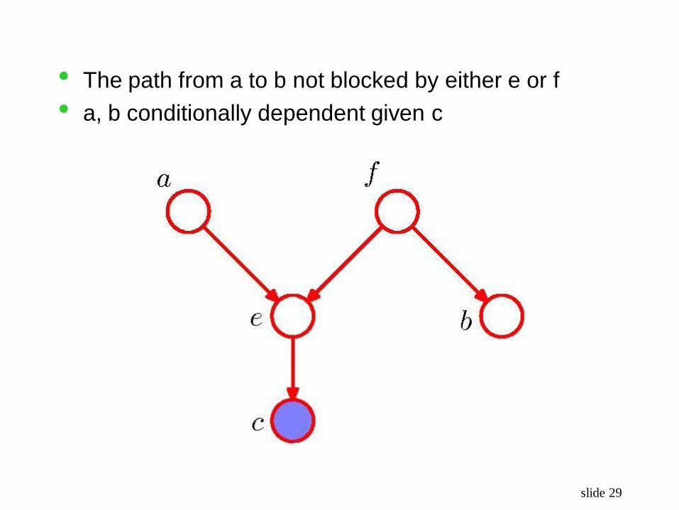
• The path from a to b not blocked by either e or f
• a, b conditionally dependent given c
slide 30
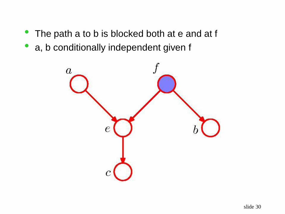
• The path a to b is blocked both at e and at f
• a, b conditionally independent given f
slide 31
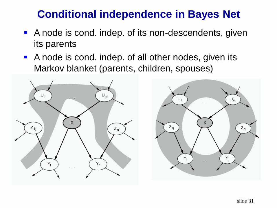
Conditional independence in Bayes Net
A node is cond. indep. of its non-descendents, given
its parents
A node is cond. indep. of all other nodes, given its
Markov blanket (parents, children, spouses)

slide 32
Compactness of Bayes net
• A Bayes net encodes a joint distribution, often with
far less parameters
• A full joint table needs kN parameters (N variables, k
values per variable)
grows exponentially with N
• If the Bayes net is sparse, e.g. each node has at
most M parents (M<<N), only needs O(NkM)
grows linearly with N
can’t have too many parents, though

slide 33
Where are we now?
• We defined a Bayes net, using small number of
parameters, to describe the joint probability
• Any joint probability can be computed as
P(x1,…xN) = i P(xi | parents(xi))
• The above joint probability can be computed in time
linear with the number of nodes N
• With this joint distribution, we can compute any
conditional probability P(Q | E), thus we can perform
any inference
• How?

slide 34
Inference by enumeration
joint matching Q AND E P(joint)
P(Q|E) =
joint matching E P(joint)
B E
A
J M
P(B)=0.001
P(A | B, E)=0.95
P(A | B, ~E)=0.94
P(A | ~B, E)=0.29
P(A | ~B, ~E)=0.001
P(E)=0.002
P(J|A)=0.9
P(J|~A)=0.05
P(M|A)=0.7
P(M|~A)=0.01
For example P(B | J, ~M)
1. Compute P(B,J,~M)
2. Compute P(J, ~M)
3. Return P(B,J,~M)/P(J,~M)

slide 35
Inference by enumeration
joint matching Q AND E P(joint)
P(Q|E) =
joint matching E P(joint)
B E
A
J M
P(B)=0.001
P(A | B, E)=0.95
P(A | B, ~E)=0.94
P(A | ~B, E)=0.29
P(A | ~B, ~E)=0.001
P(E)=0.002
P(J|A)=0.9
P(J|~A)=0.05
P(M|A)=0.7
P(M|~A)=0.01
For example P(B | J, ~M)
1. Compute P(B,J,~M)
2. Compute P(J, ~M)
3. Return P(B,J,~M)/P(J,~M)
Compute the joint (4 of them)
P(B,J,~M,A,E)
P(B,J,~M,A,~E)
P(B,J,~M,~A,E)
P(B,J,~M,~A,~E)
Each is O(N) for sparse graph P(x1,…xN) = i P(xi | parents(xi))
Sum them up

slide 36
Inference by enumeration
joint matching Q AND E P(joint)
P(Q|E) =
joint matching E P(joint)
B E
A
J M
P(B)=0.001
P(A | B, E)=0.95
P(A | B, ~E)=0.94
P(A | ~B, E)=0.29
P(A | ~B, ~E)=0.001
P(E)=0.002
P(J|A)=0.9
P(J|~A)=0.05
P(M|A)=0.7
P(M|~A)=0.01
For example P(B | J, ~M)
1. Compute P(B,J,~M)
2. Compute P(J, ~M)
3. Return P(B,J,~M)/P(J,~M)
Compute the joint (8 of them)
P(J,~M, B,A,E)
P(J,~M, B,A,~E)
P(J,~M, B,~A,E)
P(J,~M, B,~A,~E)
P(J,~M, ~B,A,E)
P(J,~M, ~B,A,~E)
P(J,~M, ~B,~A,E)
P(J,~M, ~B,~A,~E)
Each is O(N) for sparse graph
P(x1,…xN) = i P(xi | parents(xi))
Sum them up

slide 37
Inference by enumeration
joint matching Q AND E P(joint)
P(Q|E) =
joint matching E P(joint)
B E
A
J M
P(B)=0.001
P(A | B, E)=0.95
P(A | B, ~E)=0.94
P(A | ~B, E)=0.29
P(A | ~B, ~E)=0.001
P(E)=0.002
P(J|A)=0.9
P(J|~A)=0.05
P(M|A)=0.7
P(M|~A)=0.01
For example P(B | J, ~M)
1. Compute P(B,J,~M)
2. Compute P(J, ~M)
3. Return P(B,J,~M)/P(J,~M)
Sum up 4 joints
Sum up 8 joints
In general if there are
N variables, while
evidence contains j
variables, how many
joints to sum up?
slide 38
Inference by enumeration
• In general if there are N variables, while evidence
contains j variables, and each variable has k values,
how many joints to sum up?
slide 39
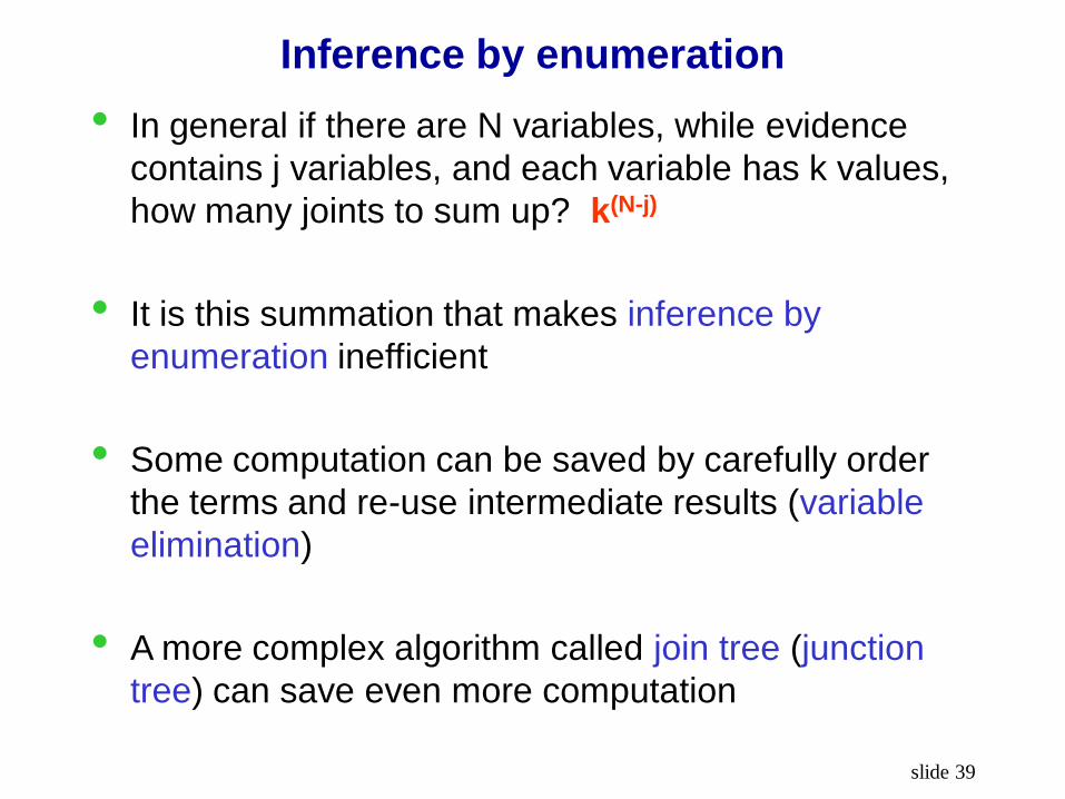
Inference by enumeration
• In general if there are N variables, while evidence
contains j variables, and each variable has k values,
how many joints to sum up? k(N-j)
• It is this summation that makes inference by
enumeration inefficient
• Some computation can be saved by carefully order
the terms and re-use intermediate results (variable
elimination)
• A more complex algorithm called join tree (junction
tree) can save even more computation

slide 40
Inference by enumeration
• In general if there are N variables, while evidence
contains j variables, and each variable has k values,
how many joints to sum up? k(N-j)
• It is this summation that makes inference by
enumeration inefficient
• Some computation can be saved by carefully order
the terms and re-use intermediate results (variable
elimination)
• A more complex algorithm called join tree (junction
tree) can save even more computation
slide 41
Approximate inference by sampling
• Inference can be done approximately by sampling
• General sampling approach:
Generate many, many samples (each sample is
a complete assignment of all variables)
Count the fraction of samples matching query
and evidence
As the number of samples approaches , the
fraction converges to the posterior
P(query | evidence)
• We’ll see 3 sampling algorithms (there are more…)
1. Simple sampling
2. Likelihood weighting
3. Gibbs sampler

slide 42
1. Simple sampling
• This BN defines a joint distribution
• Can you generate a set of samples that have the
same underlying joint distribution?
B E
A
J M
P(B)=0.001
P(A | B, E)=0.95
P(A | B, ~E)=0.94
P(A | ~B, E)=0.29
P(A | ~B, ~E)=0.001
P(E)=0.002
P(J|A)=0.9
P(J|~A)=0.05
P(M|A)=0.7
P(M|~A)=0.01

slide 43
1. Simple sampling
1. Sample B: x=rand(0,1). If (x<0.001) B=true else B=false
2. Sample E: x=rand(0,1). If (x<0.002) E=true else E=false
3. If (B==true and E==true) sample A ~ {0.95, 0.05}
elseif (B==true and E==false) sample A ~ {0.94, 0.06}
elseif (B==false and E==false) sample A ~ {0.29, 0.71}
else sample A ~ {0.001, 0.999}
4. Similarly sample J
5. Similarly sample M
This generates
one sample.
Repeat to generate
more samples
B E
A
J M
P(B)=0.001
P(A | B, E)=0.95
P(A | B, ~E)=0.94
P(A | ~B, E)=0.29
P(A | ~B, ~E)=0.001
P(E)=0.002
P(J|A)=0.9
P(J|~A)=0.05
P(M|A)=0.7
P(M|~A)=0.01

slide 44
1. Inference with simple sampling
B E
A
J M
• Say we want to infer B, given E, M, i.e. P(B | E, M)
• We generate tons of samples
• Keep those samples with E=true and M=true, throw
away others
• In the ones we keep (N of them), count the ones with
B=true, i.e. those fit our query (N1)
• We return an estimate of
P(B | E, M) N1 / N
• The quality of this estimate improves
as we sample more
• You should be able to generalize
the method to arbitrary BN
P(E)=0.002

slide 45
1. Inference with simple sampling
B E
A
J M
• Say we want to infer B, given E, M, i.e. P(B | E, M)
• We generate tons of samples
• Keep those samples with E=true and M=true, throw
away others
• In the ones we keep (N of them), count the ones with
B=true, i.e. those fit our query (N1)
• We return an estimate of
P(B | E, M) N1 / N
• The quality of this estimate improves
as we sample more
P(E)=0.002
Can you see a problem
with simple sampling?
P(B | E, M)
slide 46
1. Inference with simple sampling
B E
A
J M
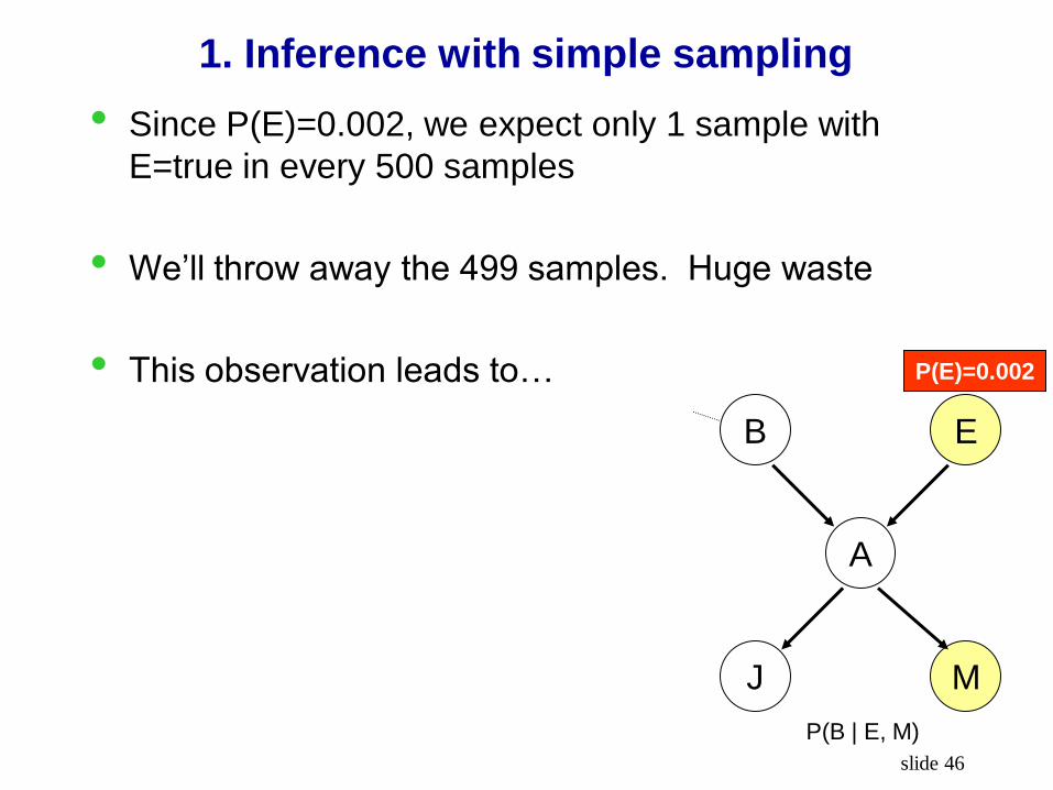
• Since P(E)=0.002, we expect only 1 sample with
E=true in every 500 samples
• We’ll throw away the 499 samples. Huge waste
• This observation leads to…
P(E)=0.002
P(B | E, M)
slide 47
2. Likelihood weighting
B E
A
J M
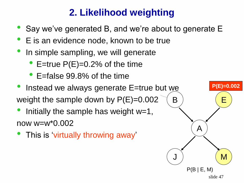
• Say we’ve generated B, and we’re about to generate E
• E is an evidence node, known to be true
• In simple sampling, we will generate
• E=true P(E)=0.2% of the time
• E=false 99.8% of the time
• Instead we always generate E=true but we
weight the sample down by P(E)=0.002
• Initially the sample has weight w=1,
now w=w*0.002
• This is ‘virtually throwing away’
P(E)=0.002
P(B | E, M)

slide 48
2. Likelihood weighting
B E
A
J M
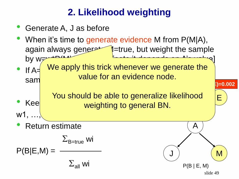
• Generate A, J as before
• When it’s time to generate evidence M from P(M|A),
again always generate M=true, but weight the sample
by w=w*P(M|A) [note it depends on A’s value]
• If A=true and P(M|A)=0.7, the final weight for this
sample is w=0.002 * 0.7
• Keep all samples, each with weight
w1, …, wN
• Return estimate
B=true wi
P(B|E,M) =
all wi
P(E)=0.002
P(B | E, M)
slide 49
2. Likelihood weighting
B E
A
J M
• Generate A, J as before
• When it’s time to generate evidence M from P(M|A),
again always generate M=true, but weight the sample
by w=w*P(M|A) [note it depends on A’s value]
• If A=true and P(M|A)=0.7, the final weight for this
sample is w=0.002 * 0.7
• Keep all samples, each with weight
w1, …, wN
• Return estimate
B=true wi
P(B|E,M) =
all wi
P(E)=0.002
P(B | E, M)
We apply this trick whenever we generate the
value for an evidence node.
You should be able to generalize likelihood
weighting to general BN.

slide 50
3. Gibbs sampler
Gibbs sampler is the simplest method in the family of
Markov Chain Monte Carlo (MCMC) methods
1. Start from an arbitrary sample, but fix evidence
nodes to their observed values, e.g.
(B=true, E=true, A=false, J=false, M=true)
2. For each hidden node X, fixing all other nodes,
resample its value from
P(X=x | Markov-blanket(X))
For example, we sample B from
P(B | E=true, A=false)
Update with its new sampled value,
and move on to A, J.
3. We now have a new sample.
Repeat from step 2.
B E
A
J M
P(B | E, M)

slide 51
3. Gibbs sampler
• Keep all samples. P(B | E, M) is the fraction with
B=true
• In general, P(X=x | Markov-blanket(X))
P(X=x | parents(X)) * Yjchildren(X) P(yj | parents(Yj))
Compute the above for X=x1,…,xk,
then normalize
• ‘burn-in’: do not use the
first Nb samples (e.g. Nb=1000) B E
A
J M
P(B | E, M)
Where X=x

slide 52
Parameter (CPT) learning for BN
• Where do you get these CPT numbers?
Ask domain experts, or
Learn from data
B E
A
J M
P(B)=0.001
P(A | B, E)=0.95
P(A | B, ~E)=0.94
P(A | ~B, E)=0.29
P(A | ~B, ~E)=0.001
P(E)=0.002
P(J|A)=0.9
P(J|~A)=0.05
P(M|A)=0.7
P(M|~A)=0.01

slide 53
Parameter (CPT) learning for BN
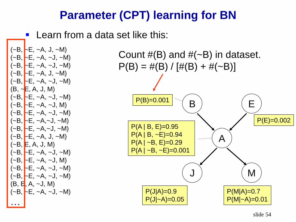
Learn from a data set like this:
B E
A
J M
P(B)=0.001
P(A | B, E)=0.95
P(A | B, ~E)=0.94
P(A | ~B, E)=0.29
P(A | ~B, ~E)=0.001
P(E)=0.002
P(J|A)=0.9
P(J|~A)=0.05
P(M|A)=0.7
P(M|~A)=0.01
(~B, ~E, ~A, J, ~M)
(~B, ~E, ~A, ~J, ~M)
(~B, ~E, ~A, ~J, ~M)
(~B, ~E, ~A, J, ~M)
(~B, ~E, ~A, ~J, ~M)
(B, ~E, A, J, M)
(~B, ~E, ~A, ~J, ~M)
(~B, ~E, ~A, ~J, M)
(~B, ~E, ~A, ~J, ~M)
(~B, ~E, ~A,~J, ~M)
(~B, ~E, ~A,~J, ~M)
(~B, ~E, ~A, J, ~M)
(~B, E, A, J, M)
(~B, ~E, ~A, ~J, ~M)
(~B, ~E, ~A, ~J, M)
(~B, ~E, ~A, ~J, ~M)
(~B, ~E, ~A, ~J, ~M)
(B, E, A, ~J, M)
(~B, ~E, ~A, ~J, ~M)
…
How to learn this CPT?
slide 54
Parameter (CPT) learning for BN
Learn from a data set like this:
B E
A
J M
P(B)=0.001
P(A | B, E)=0.95
P(A | B, ~E)=0.94
P(A | ~B, E)=0.29
P(A | ~B, ~E)=0.001
P(E)=0.002
P(J|A)=0.9
P(J|~A)=0.05
P(M|A)=0.7
P(M|~A)=0.01
(~B, ~E, ~A, J, ~M)
(~B, ~E, ~A, ~J, ~M)
(~B, ~E, ~A, ~J, ~M)
(~B, ~E, ~A, J, ~M)
(~B, ~E, ~A, ~J, ~M)
(B, ~E, A, J, M)
(~B, ~E, ~A, ~J, ~M)
(~B, ~E, ~A, ~J, M)
(~B, ~E, ~A, ~J, ~M)
(~B, ~E, ~A,~J, ~M)
(~B, ~E, ~A,~J, ~M)
(~B, ~E, ~A, J, ~M)
(~B, E, A, J, M)
(~B, ~E, ~A, ~J, ~M)
(~B, ~E, ~A, ~J, M)
(~B, ~E, ~A, ~J, ~M)
(~B, ~E, ~A, ~J, ~M)
(B, E, A, ~J, M)
(~B, ~E, ~A, ~J, ~M)
…
Count #(B) and #(~B) in dataset.
P(B) = #(B) / [#(B) + #(~B)]

slide 55
Parameter (CPT) learning for BN
Learn from a data set like this:
B E
A
J M
P(B)=0.001
P(A | B, E)=0.95
P(A | B, ~E)=0.94
P(A | ~B, E)=0.29
P(A | ~B, ~E)=0.001
P(E)=0.002
P(J|A)=0.9
P(J|~A)=0.05
P(M|A)=0.7
P(M|~A)=0.01
(~B, ~E, ~A, J, ~M)
(~B, ~E, ~A, ~J, ~M)
(~B, ~E, ~A, ~J, ~M)
(~B, ~E, ~A, J, ~M)
(~B, ~E, ~A, ~J, ~M)
(B, ~E, A, J, M)
(~B, ~E, ~A, ~J, ~M)
(~B, ~E, ~A, ~J, M)
(~B, ~E, ~A, ~J, ~M)
(~B, ~E, ~A,~J, ~M)
(~B, ~E, ~A,~J, ~M)
(~B, ~E, ~A, J, ~M)
(~B, E, A, J, M)
(~B, ~E, ~A, ~J, ~M)
(~B, ~E, ~A, ~J, M)
(~B, ~E, ~A, ~J, ~M)
(~B, ~E, ~A, ~J, ~M)
(B, E, A, ~J, M)
(~B, ~E, ~A, ~J, ~M)
…
Count #(E) and #(~E) in dataset.
P(E) = #(E) / [#(E) + #(~E)]
slide 56
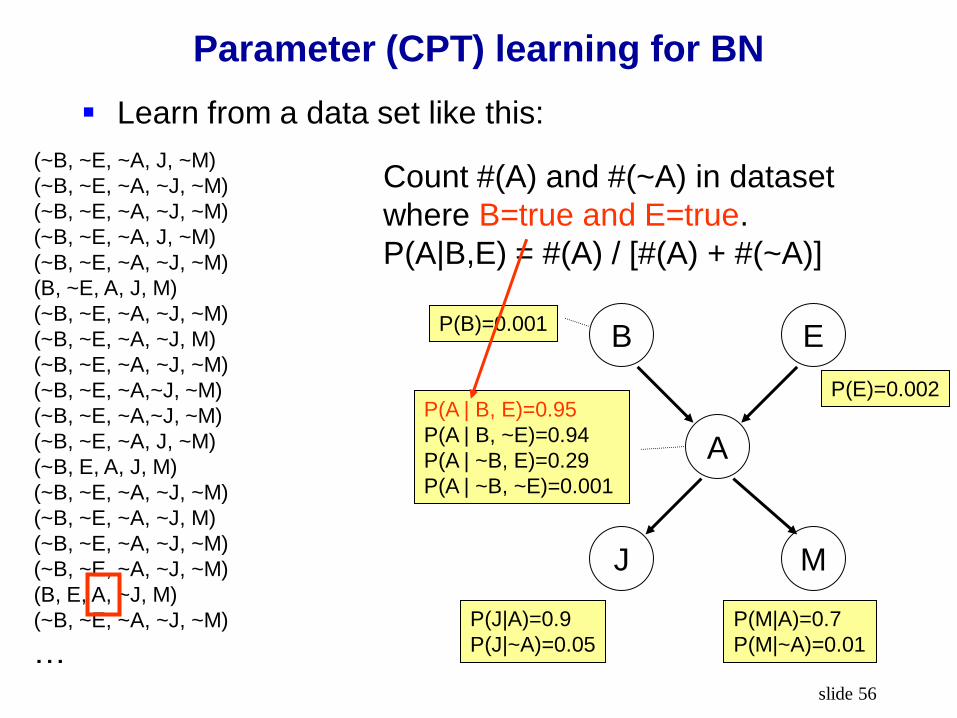
Parameter (CPT) learning for BN
Learn from a data set like this:
B E
A
J M
P(B)=0.001
P(A | B, E)=0.95
P(A | B, ~E)=0.94
P(A | ~B, E)=0.29
P(A | ~B, ~E)=0.001
P(E)=0.002
P(J|A)=0.9
P(J|~A)=0.05
P(M|A)=0.7
P(M|~A)=0.01
(~B, ~E, ~A, J, ~M)
(~B, ~E, ~A, ~J, ~M)
(~B, ~E, ~A, ~J, ~M)
(~B, ~E, ~A, J, ~M)
(~B, ~E, ~A, ~J, ~M)
(B, ~E, A, J, M)
(~B, ~E, ~A, ~J, ~M)
(~B, ~E, ~A, ~J, M)
(~B, ~E, ~A, ~J, ~M)
(~B, ~E, ~A,~J, ~M)
(~B, ~E, ~A,~J, ~M)
(~B, ~E, ~A, J, ~M)
(~B, E, A, J, M)
(~B, ~E, ~A, ~J, ~M)
(~B, ~E, ~A, ~J, M)
(~B, ~E, ~A, ~J, ~M)
(~B, ~E, ~A, ~J, ~M)
(B, E, A, ~J, M)
(~B, ~E, ~A, ~J, ~M)
…
Count #(A) and #(~A) in dataset
where B=true and E=true.
P(A|B,E) = #(A) / [#(A) + #(~A)]

slide 57
Parameter (CPT) learning for BN
Learn from a data set like this:
B E
A
J M
P(B)=0.001
P(A | B, E)=0.95
P(A | B, ~E)=0.94
P(A | ~B, E)=0.29
P(A | ~B, ~E)=0.001
P(E)=0.002
P(J|A)=0.9
P(J|~A)=0.05
P(M|A)=0.7
P(M|~A)=0.01
(~B, ~E, ~A, J, ~M)
(~B, ~E, ~A, ~J, ~M)
(~B, ~E, ~A, ~J, ~M)
(~B, ~E, ~A, J, ~M)
(~B, ~E, ~A, ~J, ~M)
(B, ~E, A, J, M)
(~B, ~E, ~A, ~J, ~M)
(~B, ~E, ~A, ~J, M)
(~B, ~E, ~A, ~J, ~M)
(~B, ~E, ~A,~J, ~M)
(~B, ~E, ~A,~J, ~M)
(~B, ~E, ~A, J, ~M)
(~B, E, A, J, M)
(~B, ~E, ~A, ~J, ~M)
(~B, ~E, ~A, ~J, M)
(~B, ~E, ~A, ~J, ~M)
(~B, ~E, ~A, ~J, ~M)
(B, E, A, ~J, M)
(~B, ~E, ~A, ~J, ~M)
…
Count #(A) and #(~A) in dataset
where B=true and E=false.
P(A|B,~E) = #(A) / [#(A) + #(~A)]

slide 58
Parameter (CPT) learning for BN
Learn from a data set like this:
B E
A
J M
P(B)=0.001
P(A | B, E)=0.95
P(A | B, ~E)=0.94
P(A | ~B, E)=0.29
P(A | ~B, ~E)=0.001
P(E)=0.002
P(J|A)=0.9
P(J|~A)=0.05
P(M|A)=0.7
P(M|~A)=0.01
(~B, ~E, ~A, J, ~M)
(~B, ~E, ~A, ~J, ~M)
(~B, ~E, ~A, ~J, ~M)
(~B, ~E, ~A, J, ~M)
(~B, ~E, ~A, ~J, ~M)
(B, ~E, A, J, M)
(~B, ~E, ~A, ~J, ~M)
(~B, ~E, ~A, ~J, M)
(~B, ~E, ~A, ~J, ~M)
(~B, ~E, ~A,~J, ~M)
(~B, ~E, ~A,~J, ~M)
(~B, ~E, ~A, J, ~M)
(~B, E, A, J, M)
(~B, ~E, ~A, ~J, ~M)
(~B, ~E, ~A, ~J, M)
(~B, ~E, ~A, ~J, ~M)
(~B, ~E, ~A, ~J, ~M)
(B, E, A, ~J, M)
(~B, ~E, ~A, ~J, ~M)
…
Count #(A) and #(~A) in dataset
where B=false and E=true.
P(A|~B,E) = #(A) / [#(A) + #(~A)]
slide 59
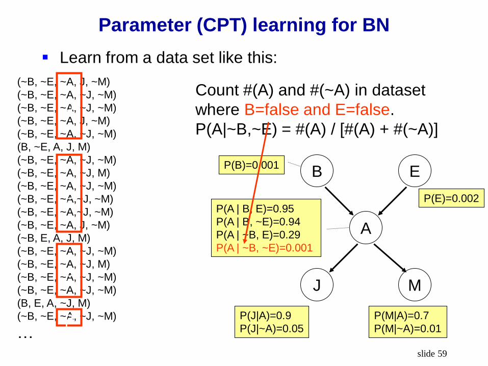
Parameter (CPT) learning for BN
Learn from a data set like this:
B E
A
J M
P(B)=0.001
P(A | B, E)=0.95
P(A | B, ~E)=0.94
P(A | ~B, E)=0.29
P(A | ~B, ~E)=0.001
P(E)=0.002
P(J|A)=0.9
P(J|~A)=0.05
P(M|A)=0.7
P(M|~A)=0.01
(~B, ~E, ~A, J, ~M)
(~B, ~E, ~A, ~J, ~M)
(~B, ~E, ~A, ~J, ~M)
(~B, ~E, ~A, J, ~M)
(~B, ~E, ~A, ~J, ~M)
(B, ~E, A, J, M)
(~B, ~E, ~A, ~J, ~M)
(~B, ~E, ~A, ~J, M)
(~B, ~E, ~A, ~J, ~M)
(~B, ~E, ~A,~J, ~M)
(~B, ~E, ~A,~J, ~M)
(~B, ~E, ~A, J, ~M)
(~B, E, A, J, M)
(~B, ~E, ~A, ~J, ~M)
(~B, ~E, ~A, ~J, M)
(~B, ~E, ~A, ~J, ~M)
(~B, ~E, ~A, ~J, ~M)
(B, E, A, ~J, M)
(~B, ~E, ~A, ~J, ~M)
…
Count #(A) and #(~A) in dataset
where B=false and E=false.
P(A|~B,~E) = #(A) / [#(A) + #(~A)]
p
p
p
p

slide 60
Parameter (CPT) learning for BN
‘Unseen event’ problem
(~B, ~E, ~A, J, ~M)
(~B, ~E, ~A, ~J, ~M)
(~B, ~E, ~A, ~J, ~M)
(~B, ~E, ~A, J, ~M)
(~B, ~E, ~A, ~J, ~M)
(B, ~E, A, J, M)
(~B, ~E, ~A, ~J, ~M)
(~B, ~E, ~A, ~J, M)
(~B, ~E, ~A, ~J, ~M)
(~B, ~E, ~A,~J, ~M)
(~B, ~E, ~A,~J, ~M)
(~B, ~E, ~A, J, ~M)
(~B, E, A, J, M)
(~B, ~E, ~A, ~J, ~M)
(~B, ~E, ~A, ~J, M)
(~B, ~E, ~A, ~J, ~M)
(~B, ~E, ~A, ~J, ~M)
(B, E, A, ~J, M)
(~B, ~E, ~A, ~J, ~M)
…
Count #(A) and #(~A) in dataset
where B=true and E=true.
P(A|B,E) = #(A) / [#(A) + #(~A)]
What if there’s no row with
(B, E, ~A, *, *) in the dataset?
Do you want to set
P(A|B,E)=1
P(~A|B,E)=0?
Why or why not?
slide 61
Parameter (CPT) learning for BN
P(X=x | parents(X)) = (frequency of x given parents)
is called the Maximum Likelihood (ML) estimate
ML estimate is vulnerable to ‘unseen event’ problem
when dataset is small
flip a coin 3 times, all heads one-sided coin?
‘Add one’ smoothing: the simplest solution.

slide 62
Smoothing CPT
‘Add one’ smoothing: add 1 to all counts
In the previous example, count #(A) and #(~A) in
dataset where B=true and E=true
P(A|B,E) = [#(A)+1] / [#(A)+1 + #(~A)+1]
If #(A)=1, #(~A)=0:
without smoothing P(A|B,E)=1, P(~A|B,E)=0
with smoothing P(A|B,E)=0.67, P(~A|B,E)=0.33
If #(A)=100, #(~A)=0:
without smoothing P(A|B,E)=1, P(~A|B,E)=0
with smoothing P(A|B,E)=0.99, P(~A|B,E)=0.01
Smoothing bravely saves you when you don’t have
enough data, and humbly hides away when you do
It’s a form of Maximum a posteriori (MAP) estimate
slide 63
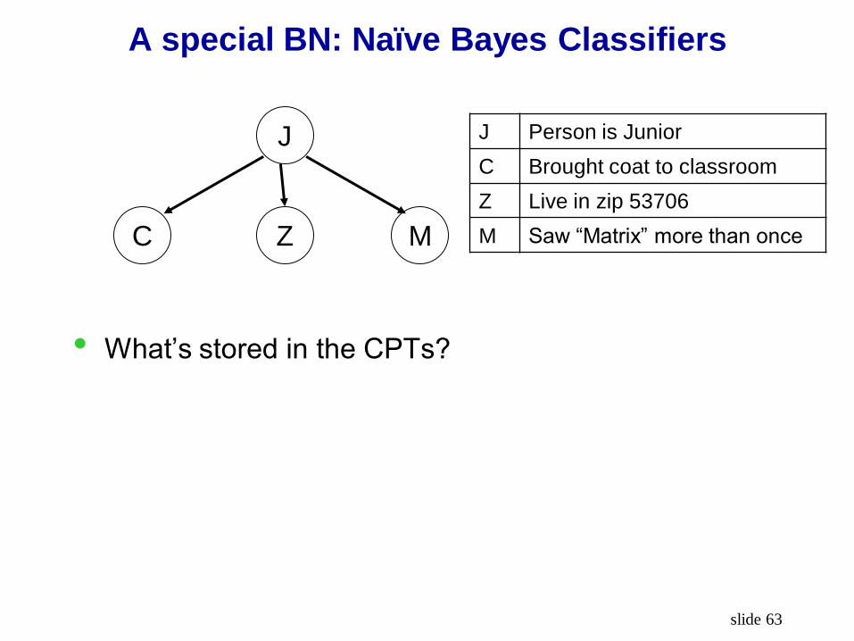
A special BN: Naïve Bayes Classifiers
J
C M Z
J Person is Junior
C Brought coat to classroom
Z Live in zip 53706
M Saw “Matrix” more than once
• What’s stored in the CPTs?
slide 64
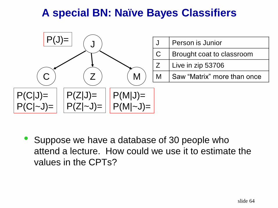
A special BN: Naïve Bayes Classifiers
J
C M Z
P(J)=
P(C|J)=
P(C|~J)=
P(Z|J)=
P(Z|~J)=
P(M|J)=
P(M|~J)=
• Suppose we have a database of 30 people who
attend a lecture. How could we use it to estimate the
values in the CPTs?
J Person is Junior
C Brought coat to classroom
Z Live in zip 53706
M Saw “Matrix” more than once

slide 65
A special BN: Naïve Bayes Classifiers
J
C M Z
P(J)=
P(C|J)=
P(C|~J)=
P(Z|J)=
P(Z|~J)=
P(M|J)=
P(M|~J)=
# Juniors
----------------------------
# people in database
# Juniors who saw M>1
---------------------------------
# Juniors
# non-juniors who saw M>1
---------------------------------------
# non-juniors
J Person is Junior
C Brought coat to classroom
Z Live in zip 53706
M Saw “Matrix” more than once

slide 66
A special BN: Naïve Bayes Classifiers
J
C M Z
P(J)=
P(C|J)=
P(C|~J)=
P(Z|J)=
P(Z|~J)=
P(M|J)=
P(M|~J)=
• A new person showed up at class wearing an “I live
right above the Union Theater where I saw Matrix
every night” overcoat.
• What’s the probability that the person is a Junior?
J Person is Junior
C Brought coat to classroom
Z Live in zip 53706
M Saw “Matrix” more than once

slide 67
Is the person a junior?
• Input (evidence): C, Z, M
• Output (query): J
P(J|C,Z,M)
= P(J,C,Z,M) / P(C,Z,M)
= P(J,C,Z,M) / [P(J,C,Z,M)+P(~J,C,Z,M)]
where
P(J,C,Z,M)=P(J)P(C|J)P(Z|J)P(M|J)
P(~J,C,Z,M)=P(~J)P(C|~J)P(Z|~J)P(M|~J)

slide 68
BN example: Naïve Bayes
• A special structure:
a ‘class’ node y at root, want P(y|x1…xN)
evidence nodes x (observed features) as leaves
conditional independence between all evidence (Assumed.
Usually wrong. Empirically OK)
y
x1 xN x2 …
slide 69
What you should know
• Inference with joint distribution
• Problems of joint distribution
• Bayes net: representation (nodes, edges, CPT) and
meaning
• Compute joint probabilities from Bayes net
• Inference by enumeration
• Inference by sampling
Simple sampling, likelihood weighting, Gibbs
• CPT parameter learning from data
• Naïve Bayes