Basis Volatilities of Corn and Soybean in

Spatially Separated Markets: The Effect of

Ethanol Demand

Anton Bekkerman, Montana State UniversityDenis Pelletier, North Carolina State University

Selected Paper prepared for presentation at the Agricultural and AppliedEconomics Association’s 2009 AAEA & ACCI Joint Annual Meeting,

Milwaukee, WI, July 26-28, 2009.

Copyright 2009 by Anton Bekkerman. All rights reserved. Readers may makeverbatim copies of this document for non-commercial purposes by any means,

provided this copyright notice appears on all such copies.

Basis Volatilities of Corn and Soybean in

Spatially Separated Markets: The Effect of

Ethanol Demand

Anton Bekkerman, Denis Pelletier*

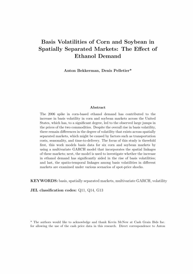
Abstract

The 2006 spike in corn-based ethanol demand has contributed to theincrease in basis volatility in corn and soybean markets across the UnitedStates, which has, to a significant degree, led to the observed large jumps inthe prices of the two commodities. Despite the overall rise in basis volatility,there remain differences in the degree of volatility that exists across spatiallyseparated markets, which might be caused by factors such as transportationcosts, seasonality, and time-to-delivery. The focus of this study is threefoldfirst, this work models basis data for six corn and soybean markets byusing a multivariate GARCH model that incorporates the spatial linkagesof these markets; next, the model is used to investigate whether the increasein ethanol demand has significantly aided in the rise of basis volatilities;and last, the spatio-temporal linkages among basis volatilities in differentmarkets are examined under various scenarios of spot-price shocks.

KEYWORDS: basis, spatially separated markets, multivariate GARCH, volatility

JEL classification codes: Q11, Q14, G13

* The authors would like to acknowledge and thank Kevin McNew at Cash Grain Bids Inc.for allowing the use of the cash price data in this research. Direct correspondence to Anton

Bekkerman. Email: anton.bekkerman@montana.edu

Basis Volatilities of Corn and Soybean in

Spatially Separated Markets: The Effect of

Ethanol Demand

Basis is an important concept in agricultural marketing, because it is a useful

tool for hedging risk for both buyers and sellers of commodities. This is primarily

because of the significantly decreased amount of variability that basis exhibits

relative to that observed in the futures prices of a commodity. Since basis is

the difference between the local cash price and the futures price for a particular

commodity, risk hedgers can take advantage of the reduced variability that is

associated with these differences.1 This smaller variability implies a significant

decrease in risk that a buyer or seller faces when purchasing futures contracts.

Accordingly, a change in market conditions that would increase the variability of

basis would decrease the ability to hedge price risk.

In August 2005, the U.S. government passed the Energy Policy Act of 2005,

which increased the number of tax incentives and loan guarantees for producers

of alternative energy sources, as well as increased the required amount of biofuel

(mainly ethanol) that must be mixed with gasoline within the United States.

Accordingly, this bill has led to a significant increase in the demand for ethanol-

based fuel production, and accordingly for corn. This has raised the price of corn

and the acreage that was dedicated to growing the crop (United States Department

1Specifically, hedgers will choose to take two opposite positions: one in the cash market andanother in the futures market.

of Agriculture (USDA-NASS)). Consequentially, this has reduced the planting and

production of soybeans, which is a crop that can be planted on the same land as

corn. In effect, the reduction of the supply of soybeans has, too, significantly raised

the price of this commodity. As shown in Figure 1 and Figure 2, the changes in

futures prices were rapid and with significant variability. This implies that unless

spot prices at local markets are perfectly correlated with futures prices, there is

an increase in the probability that the basis for the individual markets may have

become more volatile as well.

Another important aspect of basis volatility analysis is the transmission of

changes in basis across linked markets. In the United States, some markets are

net exporters of corn and soybeans, while some are net importers. For example,

a market in Iowa is a large producer of corn and soybeans, and Texas, where

the livestock industry is prominent, is a large consumer of these crops. We

might, then, assume that these markets are linked by the transport of corn and

soybeans. Accounting for these spatial linkages can be important for developing a

specification that appropriately models basis volatility in economically connected

markets.

Although there has been research that attempts to explain factors affecting

basis and forecast future basis, none attempts to directly model basis volatility.

Using a multivariate generalized autoregressive conditionally heteroskedastic

(GARCH) specification, this study seeks to appropriately model the volatility

structure of basis in spatially separated U.S. markets. After this model is

identified, it is used to determine the effects of the increase in the demand for

ethanol on the basis volatility of corn and soybeans. Prediction analysis motivates

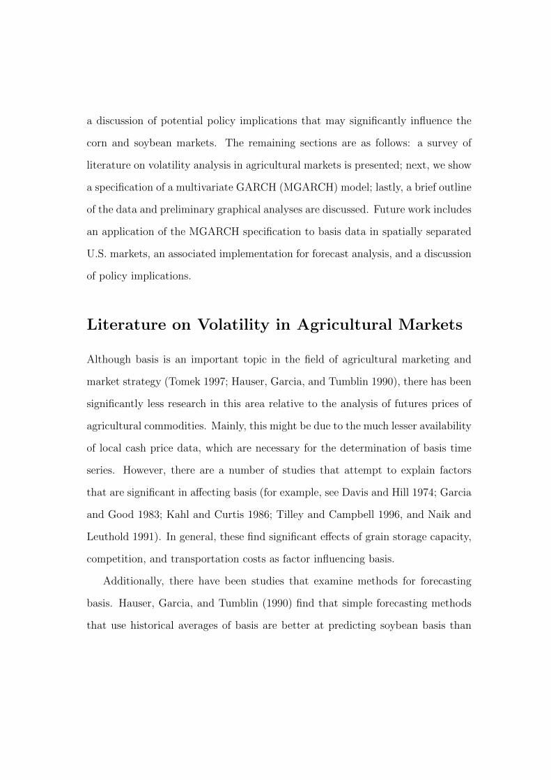
a discussion of potential policy implications that may significantly influence the

corn and soybean markets. The remaining sections are as follows: a survey of

literature on volatility analysis in agricultural markets is presented; next, we show

a specification of a multivariate GARCH (MGARCH) model; lastly, a brief outline

of the data and preliminary graphical analyses are discussed. Future work includes

an application of the MGARCH specification to basis data in spatially separated

U.S. markets, an associated implementation for forecast analysis, and a discussion

of policy implications.

Literature on Volatility in Agricultural Markets

Although basis is an important topic in the field of agricultural marketing and

market strategy (Tomek 1997; Hauser, Garcia, and Tumblin 1990), there has been

significantly less research in this area relative to the analysis of futures prices of

agricultural commodities. Mainly, this might be due to the much lesser availability

of local cash price data, which are necessary for the determination of basis time

series. However, there are a number of studies that attempt to explain factors

that are significant in affecting basis (for example, see Davis and Hill 1974; Garcia

and Good 1983; Kahl and Curtis 1986; Tilley and Campbell 1996, and Naik and

Leuthold 1991). In general, these find significant effects of grain storage capacity,

competition, and transportation costs as factor influencing basis.

Additionally, there have been studies that examine methods for forecasting

basis. Hauser, Garcia, and Tumblin (1990) find that simple forecasting methods

that use historical averages of basis are better at predicting soybean basis than

more sophisticated specifications. Dhuyvetter and Kastens (1998) compared

practical methods of basis forecasting for wheat, corn, milo, and soybeans in

Kansas, and found that the optimal choice of years necessary to forecast basis

differed by crop. Taylor, Dhuyvetter, and Kastens (2006) examined the benefits

of including current market information (basis deviation from historical averages),

finding that simple forecast models that include current market information

improve post-harvest basis forecasts for wheat, soybeans, corn, and grain sorghum

in Kansas markets. Finally, Jiang and Hayenga (1997) study basis patterns in

corn and soybean markets across the United States and determine that using an

ARIMA model that incorporates seasonal patterns improves the accuracy of basis

forecasting.

However extensive the research of basis forecasting, there are no studies that

attempt to directly model the volatility of agricultural basis. Nonetheless, there

has been a significant amount of literature devoted to volatility analysis of futures

prices in agricultural commodities. We can look to this literature to examine the

factors that might be relevant in modeling basis volatility, because there is a close

relationship between basis and futures prices.

There are several aspects that have been found significant in affecting the

variability of agricultural commodity prices. Anderson (1985) that a main factor

that influences price volatilities in grain markets is seasonality. The importance

of seasonality as well as lagged volatility was also found by Kenyon et al. (1987).

Others that find the statistical significance of seasonality effects on futures price

volatility include Hennessy and Wahl (1996) and Yang and Brorsen (1993) for

corn, soybeans, and wheat, Goodwin and Schnepf (2000) for corn and wheat, and

Chatrath et al. (2002) for soybeans, corn, wheat, and cotton. Also, evidence that

lagged volatility is important was supported by Streeter and Tomek (1992) and

Chatrath et al. (2002).

Additionally, there has been research that models agricultural commodity

futures prices using various GARCH specifications. Manfredo, Leuthold, and Irwin

(2001) provide an evaluation of several methods for estimating future cash price

volatility for fed cattle, feeder cattle, and corn cash price returns using a GARCH

model, implied volatility from options, and integrated specifications. They find

that the integrated specifications provide the best forecasts when both the time

series and implied volatility data are available. Similarly, Ramirez and Fadiga

(2003) propose an asymmetric-error GARCH model and compare its forecasting

performance to the normal-error and Student-t GARCH specifications. The study

finds that when the error term is asymmetrically distributed, their model provides

improved forecasts for soybean, sorghum, and wheat futures prices.

Finally, there are two studies that provide analyses closest to the one that

is proposed for this study. Crain and Lee (1996) study the effects of thirteen

various farm programs on wheat spot and futures price volatilities between 1950 –

1993. They find that, in general, the mandatory farm programs have lowered

the volatility of wheat prices, while voluntary farm programs have increased

volatility. However, Yang, Haigh, and Leatham (2001) apply several GARCH

model specifications to corn, soybeans, wheat, oats, and cotton futures prices in

order to measure whether there was an increase in price volatility following the

agricultural liberalization policies in the FAIR Act (1996). Unlike Crain and Lee

(1996), their results indicate that there was an increase in the volatility of corn,

soybeans, and wheat prices, insignificant change in the price volatility of oats, and

a decrease in the volatility of cotton.

Specification of the M-GARCH Model

An assumption with standard time series modeling is a constant variance.

However, in financial data, including that in agricultural markets, this assumption

might not be realistic. For example, it is often observed that periods of high

market volatility are typically clustered together, indicating a strong dependence

between market factors and past variability shocks. The first model to deal with

heteroskedastic error variances was proposed by Engle (1982), spawning a large

literature on variations of the original autoregressive conditional heteroskedasticity

(ARCH) specification.2 An extension of the ARCH model is the generalized

autoregressive conditional heteroskedasticity specification (GARCH), which was

proposed by Bollerslev (1986). GARCH considers that the conditional variance

of the error process is related to both the squares of the past errors as well as

the lagged conditional variances. A standard, univariate GARCH(1,1) model is as

follows:

yt = �t"t

(1)

�2t = �o + �1y

2t−1 + �1�

2t−1

2See Bollerslev, Chou, and Kroner (1992) for a survey of these models.

where "t ∼ N(0, 1). Additionally, there has been an exhaustive literature that

has examined variations of the univariate GARCH specification (see Bollerslev,

Chou, and Kroner (1992) for a survey of GARCH models and their applications).

However, for the analysis at hand, it is necessary to consider a model that can

simultaneously analyze the relationship of volatilities in multiple markets. In this

case, a multivariate GARCH (MGARCH) model is appropriate.

Since the objective of this study is to examine basis volatility in spatially

linked markets, the MGARCH specification is a tool that is capable of explaining

the relationship between volatilities and co-volatilities in several markets. Using

the MGARCH model, it is possible to provide an appropriate analysis of posed

questions. For example, whether a shock to the volatility of the basis in a

supplier market lead an increase in basis variability in a another supplier market

or a demand market, as well as the speed at which these shocks might be

transmitted. Similarly, it possible to determine whether there is a direct (through

the conditional variance) transmission of a variability shock to another market,

or if the transmission occurs through the conditional covariances. Also, we can

consider the effects of a potential structural change, such as an increased demand

for ethanol, on basis volatility in the short- and long-run.

To define a specification of a multivariate GARCH model that can be used for

this analysis, we use the notation in Bauwens, Laurent, and Rombouts (2006).

Consider a stochastic process yt of dimension N × 1, which is conditioned on

a set of past information up to time t − 1, denoted as It−1. The process can be

modeled as follows:

yt = �t(�) + "t

(2)

"t = H1/2t (�) ⋅ zt

where �t(�) is the vector of the conditional mean, H1/2t is an N × N positive

definite matrix, and the random error term, zt, is assumed to have a mean vector

0N and a variance structure that is an identity matrix of order N . Additionally,

H1/2t is the Cholesky decomposition of Ht, which is the conditional variance matrix

of yt and can be expressed as follows:

Var(yt∣It−1) = Vart−1(yt) = Vart−1("t)

= H1/2t Vart−1(zt)(H

1/2t )

′

= Ht

The structure of the model as a whole, then, is determined by the specification of

Ht. Bauwens, Laurent, and Rombouts (2006) provides a comprehensive overview

of a number of different approaches for defining Ht. For this study, we consider

using the class of conditional correlation models, which are nonlinear combinations

of univariate GARCH models. In these models, it is possible to separately

specify the individual conditional variances and the conditional correlation matrix

between individual series. Additionally, these models do not require the estimation

of as many parameters as alternative specification, and so, might be subject to

easier estimation methods. Specifically, we consider using a dynamic conditional

correlation (DCC) model, which allow for the conditional correlation matrix to

be time-dependent.3 Following Engle (2002), the DCC(1, 1) model for Ht is as

follows:

Ht = DtRtDt (3)

where

Dt = diag(ℎ1/211t ⋅ ℎ

1/222t ⋅ ⋅ ⋅ℎ

1/2NNt) (4)

In each univariate GARCH specification, ℎiit, we specify a dummy variable that

captures the effect of an increased demand for ethanol after the year 2006. Also,

due to the significant effects of seasonality on basis, it might be necessary to

consider the inclusion of a function, s(t), that appropriately models these effects.

This is as follows:

ℎiit = !i + �i(ETH06) + is(t) + �i"2i,t−1 + �iℎii,t−1 (5)

for i = 1, . . . , N

3This is in contrast to another type of conditional correlation models, which assume a constantcorrelation matrix. See Bollerslev (1990) for a description of the constant conditional correlation(CCC) models.

Additionally, the term Rt is defined as:

Rt = diag(q−1/211,t ⋅ ⋅ ⋅ q

−1/2NN,t) ⋅Qt ⋅ diag(q

−1/211,t ⋅ ⋅ ⋅ q

−1/2NN,t) (6)

such that Qt is an N × N symmetric positive definite matrix as follows:

Qt = (1− �− �)Q+ �ut−1u′

t−1 + �Qt−1 (7)

where uit = "it/√ℎiit, Q is an N × N unconditional matrix of ut, and

� > 0

� > 0

� + � < 1

Estimation of the parameters can be performed using maximum likelihood

estimation. The log-likelihood function can be defined as follows:

LLT (�) = −1

2

T∑t=1

log ∣Ht∣ −1

2

T∑t=1

(yt − �t)′H−1

t (yt − �t) (8)

According to Engle and Sheppard (2001), consistent estimation of the DCC

model can be performed by using a two-step approach. First, it is necessary

to estimate the parameters �∗1, which is the mean and volatility, and then the

parameters �∗2 that correspond to the correlation. In each step, the estimation

yields consistent, though inefficient parameter values. However, using the set of

estimated parameters (�̂∗1, �̂∗2) as starting values in equation (8) will result in an

asymptotically efficient estimator of the parameter set, �. The quasi log-likelihood

functions that need to be estimated to obtain the parameter set (�̂∗1, �̂∗2) are as

follows:

QLL1T (�∗1) = −1

2

T∑t=1

N∑i=1

{log(ℎiit) +

(yit − �it)2

ℎiit

}(9)

QLL2T (�∗2) = −1

2

T∑t=1

{log ∣Rt∣+ [D−1

t (yt − �t)]′ ⋅R−1

t ⋅ [D−1t (yt − �t)]

}(10)

We can then use the estimate �̂ to retrieve �(�̂) and H(�̂). All estimations are

performed using the SAS software system.

U.S. Corn Markets and Soybean Markets

Data

Basis data in this research are calculated using spot prices from several major

U.S. markets and nearby futures from the Chicago Board of Trade (CBOT). For

corn, we use weekly spot price data for the following: Aberdeen, South Dakota;

Alton, Iowa; Gulf, Louisiana; Muleshoe, Texas; Guntersville, Alabama; Candor,

North Carolina; and, Western, Illinois. Soybean markets were: Aberdeen, South

Dakota; Alton, Iowa; Gulf, Louisiana; Muleshoe, Texas; Raleigh, North Carolina;

and, Western, Illinois.4 For both commodities, Western, Illinois is selected as

the central market, due to its proximity to a large port that is used to transport

commodities from major supply markets to demand markets. The data spans the

range between June 17, 1999 and January 10, 2008. Weeks during which there

4This data are supplied by Cash Grain Bids Inc. (www.cashgrainbids.com)

were missing observations were interpolated using an exponential spline method.

Summary statistics for the basis data are shown in Table 1 and for the basis

difference pairs in Table 2. The time series of corn basis is shown in Figure 3

and for soybeans in Figure 4. Additionally, the time series of basis pairs between

the central location and another market are shown in Figure 5 and Figure 6 for

corn and soybeans, respectively. Finally, the sample annualized volatility for the

corn and soybean basis are presented in Figure 7 and Figure 8. These indicate a

significant increase in basis volatility in some of the markets after 2006.

References

Bauwens, L., S. Laurent, and J. Rombouts. 2006. “Multivariate GARCH Models:

A Survey.” Journal of Applied Econometrics 21:79–109.

Bollerslev, T. 1990. “Modeling the Coherence in Short-Run Nominal Exchange

Rates: A Multivariate Generalized ARCH Model.” Review of Economics and

Statistics 72:498505.

Bollerslev, T., R. Chou, and K. Kroner. 1992. “ARCH Modeling In Finance: A

Review of the Theory and Empirical Evidence.” Journal of Econometrics 52:5–

59.

Crain, S., and J. Lee. 1996. “Volatility in Wheat Spot and Futures Markets, 1950-

1993: Government Farm Programs, Seasonality, and Causality.” The Journal of

Finance 51:325–343.

Davis, L., and L. Hill. 1974. “Spatial Price Differentials for Corn among Illinois

Country Elevators.” American Journal of Agricultural Economics 56:135–144.

Dhuyvetter, K., and T. Kastens. 1998. “Forecasting Crop Basis: Practical

Alternatives.” Proceedings of NCR-134 Conference on Applied Commodity

Price Analysis, Forecasting, and Market Risk Management.

Engle, R. 2002. “Dynamic Conditional Correlation – A Simple Class of

Multivariate GARCH Models.” Journal of Business and Economic Statistics

20:339–350.

Engle, R., and K. Sheppard. 2001. “Theoretical and Empirical Properties of

Dynamic Conditional Correlation Multivariate GARCH.” Unpublished, Mimeo,

UCSD.

Garcia, P., and D. Good. 1983. “An Analysis of the Factors Influencing the

Illinois Corn Basis, 1971–1981.” Proceedings of NCR-134 Conference on Applied

Commodity Price Analysis, Forecasting, and Market Risk Management.

Hauser, R., P. Garcia, and A. Tumblin. 1990. “Basis Expectations and Soybean

Hedging Effectiveness.” North Central Journal of Agricultural Economics

12:125–136.

Jiang, B., and M. Hayenga. 1997. “Corn and Soybean Basis Behavior and

Forecasting: Fundamental and Alternative Approaches.” Proceedings of NCR-

134 Conference on Applied Commodity Price Analysis, Forecasting, and Market

Risk Management.

Kahl, K., and C. Curtis. 1986. “A Comparative Analysis of the Corn Basis in

Feed Grain Deficit and Surplus Areas.” Review of Resources in Futures Markets

5:220–232.

Manfredo, M., R. Leuthold, and S. Irwin. 2001. “Forecasting Fed Cattle, Feeder

Cattle, and Corn Cash Price Volatility: The Accuracy of Time Series, Implied

Volatility, and Composite Approaches.” Journal of Agricultural and Applied

Economics 33:523–538.

Naik, G., and R. Leuthold. 1991. “A Note on the Factors Affecting Corn Basis

Relationships.” Southern Journal of Agricultural Economics 23:147–153.

Ramirez, O., and M. Fadiga. 2003. “Forecasting Agricultural Commodity Prices

with Asymmetric-Error GARCH Models.” Journal of Agricultural and Resource

Economics 28:71–85.

Taylor, M., K. Dhuyvetter, and T. Kastens. 2006. “Forecasting Crop Basis Using

Historical Averages Supplemented with Current Market Information.” Journal

of Agricultural and Resource Economics 31:549–567.

Tilley, D., and S. Campbell. 1996. “Performance of the Weekly Gulf-Kansas City

Hard-Red Winter Wheat Basis.” American Journal of Agricultural Economics

70:929–935.

Tomek, W. 1997. “Commodity Futures Prices as Forecasts.” Review of Agricultural

Economics 19:23–44.

United States Department of Agriculture (USDA-NASS). Various Years. “Census

of Agriculture.” www.nass.usda.gov.

Yang, J., M. Haigh, and D. Leatham. 2001. “Agricultural Liberalization Policy

and Commodity Price Volatility: A GARCH Application.” Applied Economics

Letters 8:593–598.

Table 1: Summary Statistics: Basis for Selected U.S. Markets

Market Location Obs. Mean Std. Dev. Min. Max.

Corn

Aberdeen, South Dakota 445 -0.41641 0.15828 -0.78188 0.001Alton, Iowa 445 -0.31607 0.12214 -0.85036 -0.01355Western, Illinois 445 -0.25811 0.09492 -0.73444 -0.0035Gulf, Louisiana 445 0.29317 0.13797 0.01063 0.679Muleshoe, Texas 445 0.07825 0.19821 -1.24181 0.48421Guntersville, Alabama 445 0.01872 0.18633 -0.99 0.355Candor, North Carolina 445 0.16208 0.14576 -0.151 0.503

............................................................................................

Soybeans

Aberdeen, South Dakota 447 -0.61563 0.29541 -1.59333 0.8525Alton, Iowa 447 -0.41733 0.33386 -2.02501 1.26Western, Illinois 447 -0.28807 0.2704 -2.33697 1.3625Gulf, Louisiana 447 0.34431 0.15852 -0.1915 1.445Muleshoe, Texas 447 -0.90097 0.26989 -2.64833 -0.014Raleigh, North Carolina 447 0.07856 0.15715 -0.242 1.1675

Table 2: Summary Statistics: Basis Pairs for Selected U.S. Markets

Market Location Obs. Mean Std. Dev. Min. Max.

Corn

South Dakota-Illinois 445 -0.1583 0.13436 -0.45 0.45444Iowa-Illinois 445 -0.05796 0.1075 -0.54886 0.50444Louisiana-Illinois 445 0.55128 0.15499 0.258 1.038Texas-Illinois 445 0.33636 0.18473 -0.90381 0.755Alabama-Illinois 445 0.27683 0.17364 -0.67333 0.69North Carolina-Illinois 445 0.42019 0.12991 0.07 0.83444

............................................................................................

Soybeans

South Dakota-Illinois 447 -0.32756 0.22169 -1.2725 0.84363Iowa-Illinois 447 -0.12926 0.27795 -1.72336 1.15697Louisiana-Illinois 447 0.63238 0.2312 -0.289 2.2703Texas-Illinois 447 -0.6129 0.25351 -2.64156 -0.0175North Carolina-Illinois 447 0.36663 0.23816 -0.379 2.2103

Figure 1: Corn and Soybean Futures Prices: 06/1999 - 01/2008

Figure 2: Corn and Soybean Futures Price Volatility: 06/1999 - 01/2008

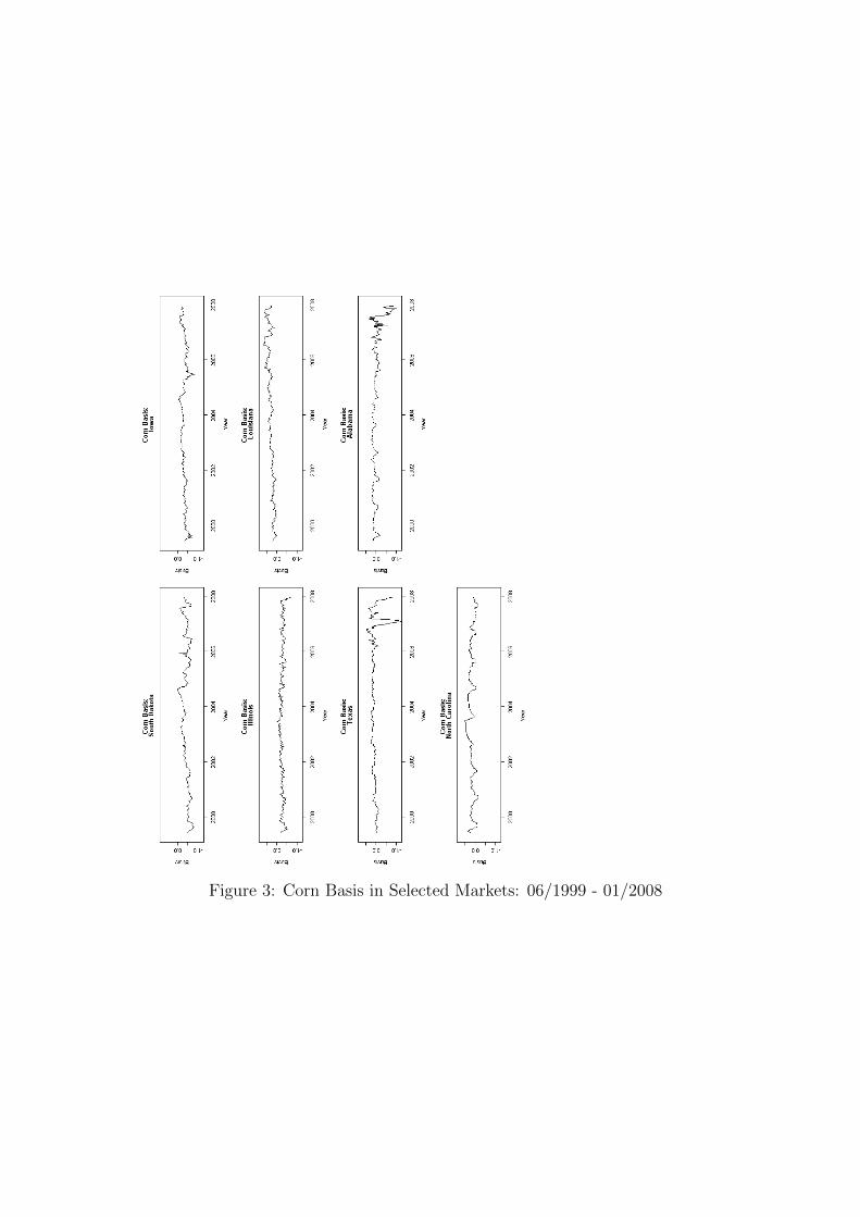
Figure 3: Corn Basis in Selected Markets: 06/1999 - 01/2008

Figure 4: Soybean Basis in Selected Markets: 06/1999 - 01/2008

Figure 5: Absolute Differences in Basis for Selected Corn Markets

Figure 6: Absolute Differences in Basis for Selected Soybean Markets

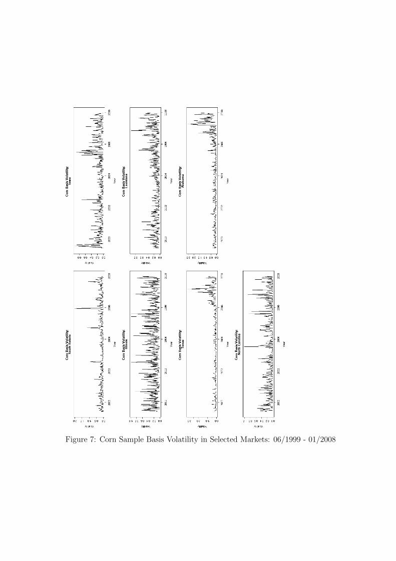
Figure 7: Corn Sample Basis Volatility in Selected Markets: 06/1999 - 01/2008

Figure 8: Soybean Sample Basis in Selected Markets: 06/1999 - 01/2008