
Basics of Stochastic Analysis
331
Basics of Stochastic Analysis c Timo Sepp¨ al¨ ainen Department of Mathematics, University of Wisconsin–Madison , Madison, Wisconsin 53706 E-mail address : [email protected]
Transcript of Basics of Stochastic Analysis

8/3/2019 Basics of Stochastic Analysis
http://slidepdf.com/reader/full/basics-of-stochastic-analysis 1/330
Basics of Stochastic Analysis
c Timo Sepp¨alainen
Department of Mathematics, University of Wisconsin–Madison,Madison, Wisconsin 53706
E-mail address : [email protected]
8/3/2019 Basics of Stochastic Analysis
http://slidepdf.com/reader/full/basics-of-stochastic-analysis 2/330
This version December 19, 2010.
The author has been supported by NSF grants and by the WisconsinAlumni Research Foundation.
Abstract. This material is for a course on stochastic analysis at UW–Madison. The text covers the development of the stochastic integral of predictable processes with respect to cadlag semimartingale integrators,It o’s formula in an open domain in R n , an existence and uniquenesstheorem for an equation of the type dX = dH + F (t, X ) dY where Y is a cadlag semimartingale, and local time and Girsanov’s theorem forBrownian motion.
The text is self-contained except for certain basics of integrationtheory and probability theory which are explained but not proved. Inaddition, the reader needs to accept without proof two basic martin-gale theorems: (i) the existence of quadratic variation for a cadlag localmartingale; and (ii) the so-called fundamental theorem of local martin-gales that states the following: given a cadlag local martingale M anda positive constant c, M can be decomposed as N + A where N and Aare cadlag local martingales, jumps of N are bounded by c, and A haspaths of bounded variation.
This text intends to provide a stepping stone to deeper books suchas Karatzas-Shreve and Protter. The hope is that this material is acces-sible to students who do not have an ideal background in analysis andprobability theory, and useful for instructors who (like the author) arenot experts on stochastic analysis.

8/3/2019 Basics of Stochastic Analysis
http://slidepdf.com/reader/full/basics-of-stochastic-analysis 3/330
Contents
Chapter 1. Measures, Integrals, and Foundations of ProbabilityTheory 1
§1.1. Measure theory and integration 1
§1.2. Basic concepts of probability theory 19Exercises 33
Chapter 2. Stochastic Processes 39
§2.1. Filtrations and stopping times 39
§2.2. Quadratic variation 49
§2.3. Path spaces, martingale property and Markov property 56§2.4. Brownian motion 63
§2.5. Poisson processes 76Exercises 80
Chapter 3. Martingales 85
§3.1. Optional stopping 87
§3.2. Inequalities and limits 91
§3.3. Local martingales and semimartingales 95
§3.4. Quadratic variation for semimartingales 97
§3.5. Doob-Meyer decomposition 102
§3.6. Spaces of martingales 105Exercises 109
Chapter 4. Stochastic Integral with respect to Brownian Motion 111
iii

8/3/2019 Basics of Stochastic Analysis
http://slidepdf.com/reader/full/basics-of-stochastic-analysis 4/330
iv Contents
Exercises 125
Chapter 5. Stochastic Integration of Predictable Processes 127
§5.1. Square-integrable martingale integrator 128
§5.2. Local square-integrable martingale integrator 155
§5.3. Semimartingale integrator 165
§5.4. Further properties of stochastic integrals 171
§5.5. Integrator with absolutely continuous Doleans measure 182Exercises 187
Chapter 6. Itˆo’s Formula 191
§6.1. Quadratic variation 191
§6.2. It o’s formula 200
§6.3. Applications of It o’s formula 208Exercises 216
Chapter 7. Stochastic Differential Equations 219
§7.1. Examples of stochastic equations and solutions 220
§7.2. Existence and uniqueness for It o equations 227
§7.3. A semimartingale equation 238
§7.4. Existence and uniqueness for a semimartingale equation 243Exercises 268
Chapter 8. Applications of Stochastic Calculus 269
§8.1. Local time 269
§8.2. Change of measure 281Exercises 286
Appendix A. Analysis 287
§A.1. Continuous, cadlag and BV functions 289
§A.2. Differentiation and integration 299Exercises 302
Appendix B. Probability 303
§B.1. General matters 303
§B.2. Construction of Brownian motion 313
Bibliography 321
Notation and Conventions 323
Index 325

8/3/2019 Basics of Stochastic Analysis
http://slidepdf.com/reader/full/basics-of-stochastic-analysis 5/330
Chapter 1
Measures, Integrals,and Foundations of Probability Theory
In this chapter we sort out the integrals one typically encounters in courseson calculus, analysis, measure theory, probability theory and various appliedsubjects such as statistics and engineering. These are the Riemann inte-gral, the Riemann-Stieltjes integral, the Lebesgue integral and the Lebesgue-Stieltjes integral. The starting point is the general Lebesgue integral on anabstract measure space. The other integrals are special cases, even though
they have denitions that look different.This chapter is not a complete treatment of the basics of measure theory.
It provides a brief unied explanation for readers who have prior familiaritywith various notions of integration. To avoid unduly burdening this chapter,many technical matters that we need later in the book have been relegatedto the appendix. For details that we have omitted and for proofs the readershould turn to any of the standard textbook sources, such as Folland [ 6 ].
In the second part of the chapter we go over the measure-theoretic foun-dations of probability theory. Readers who know basic measure theory andmeasure-theoretic probability can safely skip this chapter.
1.1. Measure theory and integration
A space X is in general an arbitrary set. For integration, the space musthave two additional structural elements, namely a σ-algebra and a measure.
1
8/3/2019 Basics of Stochastic Analysis
http://slidepdf.com/reader/full/basics-of-stochastic-analysis 6/330
2 1. Measures, Integrals, and Foundations of Probability Theory
1.1.1. σ-algebras. Suppose Ais a collection of subsets of X . (Terms such
as class, collection and family are used as synonyms for set to avoid speakingof “sets of sets,” or even “sets of sets of sets.”) Then Ais a σ-algebra (alsocalled a σ-eld ) if it has these properties:
(i) X ∈ Aand ∅ ∈ A.(ii) If A∈ Athen also Ac
∈ A.(iii) If Aiis a sequence of sets in A, then also their union i Ai is an
element of A.
The restriction to countable unions in part (iii) is crucial. Unions overarbitrarily large collections of sets are not permitted. On the other hand, if part (iii) only permits nite unions, then Ais called an algebra of sets, but
this is not rich enough. .A pair ( X, A) where X is a space and Ais a σ-algebra on X is called
a measurable space . The elements of Aare called measurable sets . Suppose(X, A) and ( Y, B) are two measurable spaces and f : X →Y is a map(another term for a function) from X into Y . Then f is measurable if forevery B∈ B, the inverse image
f −1(B ) = x∈X : f (x)∈B= f ∈Blies in A. Measurable functions are the fundamental object in measuretheory. Measurability is preserved by composition f g of functions.
In nite or countable spaces the useful σ-algebra is usually the power set 2X which is the collection of all subsets of X . Not so in uncountable spaces.Furthermore, the important σ-algebras are usually very complicated so thatit is impossible to give a concise criterion for testing whether a given set isa member of the σ-algebra. The preferred way to dene a σ-algebra is togenerate it by a smaller collection of sets that can be explicitly described.This procedure is analogous to spanning a subspace of a vector space with agiven set of vectors. Except that the generated σ-algebra usually lacks thekind of internal description that vector subspaces have as the set of nitelinear combinations of basis vectors. Generation of σ-algebras is based onthis lemma whose proof the reader should ll in as an exercise, if this materialis new.
Lemma 1.1. Let Γ be a family of σ-algebras on a space X . Then theintersection
C=
A∈ΓA
is also a σ-algebra.
Let E be an arbitrary collection of subsets of X . The σ-algebra generated by E , denoted by σ(E ), is by denition the intersection of all σ-algebras on
8/3/2019 Basics of Stochastic Analysis
http://slidepdf.com/reader/full/basics-of-stochastic-analysis 7/330
1.1. Measure theory and integration 3
X that contain E . This intersection is well-dened because there is always
at least one σ-algebra on X that contains E , namely the power set 2 X . Anequivalent characterization of σ(E ) is that it satises these three properties:(i) σ(E )⊇ E , (ii) σ(E ) is a σ-algebra on X , and (iii) if Bis any σ-algebra onX that contains E , then σ(E )⊆ B. This last point justies calling σ(E ) thesmallest σ-algebra on X that contains E .
A related notion is a σ-algebra generated by collection of functions.Suppose ( Y, H) is a measurable space, and Φ is a collection of functionsfrom X into Y . Then the σ-algebra generated by Φ is dened by
(1.1) σ(Φ) = σ f ∈B: f ∈Φ, B ∈ H.
σ(Φ) is the smallest σ-algebra that makes all the functions in Φ measurable.
Example 1.2 (Borel σ-algebras) . If X is a metric space, then the Borel σ-eld BX is the smallest σ-algebra on X that contains all open sets. Themembers of BX are called Borel sets . We also write B(X ) when subscriptsbecome clumsy.
It is often technically convenient to have different generating sets for aparticular σ-algebra. For example, the Borel σ-algebra BR of the real lineis generated by either one of these classes of intervals:
(a, b] :−∞< a < b < ∞ and (−∞, b) : −∞< b < ∞.We shall also need the Borel σ-algebra B[−∞,∞] of the extended real line
[−∞, ∞]. We dene this as the smallest σ-algebra that contains all Borel setson the real line and the singletons −∞and ∞. This σ-algebra is alsogenerated by the intervals [−∞, b] : b∈R . It is possible to dene a metricon [−∞, ∞] such that this σ-algebra is the Borel σ-algebra determined bythe metric.
When we speak of real-valued or extended real-valued measurable func-tions on an arbitrary measurable space ( X, A), we always have in mind theBorel σ-algebra on R and [−∞, ∞]. One can then check that measurabilityis preserved by algebraic operations ( f ±g, fg , f /g , whenever these are well-dened) and by pointwise limits and suprema of sequences: if f n : n∈N is a sequence of real-valued measurable functions, then for example the func-tions
g(x) = supn∈N
f n (x) and h(x) = limn→∞
f n (x)
are measurable. The set N above is the set of natural numbers N =
1, 2, 3, . . . . Thus measurability is a more robust property than other fa-miliar types of regularity, such as continuity or differentiability, that are notin general preserved by pointwise limits.

8/3/2019 Basics of Stochastic Analysis
http://slidepdf.com/reader/full/basics-of-stochastic-analysis 8/330
4 1. Measures, Integrals, and Foundations of Probability Theory
If (X, BX ) is a metric space with its Borel σ-algebra, then every continu-
ous function f : X →R is measurable. The denition of continuity impliesthat for any open G ⊆R , f −1(G) is an open set in X , hence a memberof BX . Since the open sets generate BR , this suffices for concluding thatf −1(B )∈ BX for all Borel sets B⊆R .
Example 1.3 (Product σ-algebras) . Of great importance for probabilitytheory are product σ-algebras. Let I be an arbitrary index set, and foreach i∈ I let (X i , Ai ) be a measurable space. The Cartesian product spaceX = i∈I X i is the space of all functions x : I → i∈I X i such thatx(i)∈X i for each i. Alternate notation for x(i) is x i . Coordinate projection maps on X are dened by f i (x) = x i , in other words f i maps X onto X i byextracting the i-coordinate of the
I -tuple x. The product σ-algebra i
∈I Ai
is by denition the σ-algebra generated by the coordinate projections f i :i∈ I.
1.1.2. Measures. Let us move on to discuss the second fundamental in-gredient of integration. Let ( X, A) be a measurable space. A measure is afunction µ : A →[0, ∞] that satises these properties:
(i) µ(∅) = 0.(ii) If Aiis a sequence of sets in Asuch that Ai ∩A j = ∅for all i = j
(pairwise disjoint is the term), then
µi
Ai =i
µ(Ai ).
Property (ii) is called countable additivity . It goes together with the factthat σ-algebras are closed under countable unions, so there is no issue aboutwhether the union i Ai is a member of A. The triple ( X, A, µ) is called ameasure space .
If µ(X ) < ∞ then µ is a nite measure . If µ(X ) = 1 then µ is a prob-ability measure . Innite measures arise naturally. The ones we encountersatisfy a condition called σ-niteness: µ is σ-nite if there exists a sequenceof measurable sets V isuch that X = V i and µ(V i ) < ∞ for all i. Ameasure dened on a Borel σ-algebra is called a Borel measure .
Example 1.4. Suppose X = x i : i∈
N is a countable space, and leta i : i∈N be a sequence of nonnegative real numbers. Then
µ(A) =i:x i∈A
a i
denes a σ-nite (or nite, if a i < ∞) measure on the σ-algebra 2 X of allsubsets of X .
8/3/2019 Basics of Stochastic Analysis
http://slidepdf.com/reader/full/basics-of-stochastic-analysis 9/330
1.1. Measure theory and integration 5
The example shows that to dene a measure on a countable space, one
only needs to specify the measures of the singletons, and the rest followsby countable additivity. Again, things are more complicated in uncountablespaces. For example, we would like to have a measure m on the Borel sets of the real line with the property that the measure m(I ) of an interval I is thelength of the interval. (This measure is known as the Lebesgue measure.)But then the measure of any singleton must be zero. So there is no way toconstruct the measure by starting with singletons.
Since it is impossible to describe every element of a σ-algebra, it iseven more impossible to give a simple explicit formula for the measure of every measurable set. Consequently we need a theorem that “generates” ameasure from some modest ingredients that can be explicitly written down.
Here is a useful one.First, a class S of subsets of X is a semialgebra if it has these properties:
(i) ∅ ∈ S (ii) If A, B ∈ S then also A ∩B∈ S .
(iii) If A∈ S , then Ac is a nite disjoint union of elements of S .A good example on the real line to keep in mind is
(1.2) S = (a, b] :−∞ ≤a ≤b < ∞∪(a, ∞) : −∞ ≤a < ∞.This semialgebra generates BR .
Theorem 1.5. Let
S be a semialgebra, and µ0 :
S →[0,
∞] a function with
these properties:(i) µ0(∅) = 0
(ii) If A ∈ S is a nite disjoint union of sets B1, . . . , B n in S , then µ0(A) = µ0(B i ).
(iii) If A∈ S is a countable disjoint union of sets B1, B2, . . . , B n , . . . in
S , then µ0(A) ≤ µ0(B i ).
Assume furthermore that there exists a sequence of sets Aiin S such that X = Ai and µ0(Ai ) < ∞ for all i. Then there exists a unique measure µon the σ-algebra σ(S ) such that µ = µ0 on S .
This theorem is proved by rst extending µ0
to the algebra generatedby S , and by then using the so-called Caratheodory Extension Theorem togo from the algebra to the σ-algebra. With Theorem 1.5 we can describe alarge class of measures on R .
Example 1.6 (Lebesgue-Stieltjes measures) . Let F be a nondecreasing,right-continuous real-valued function on R . For intervals ( a, b], dene
µ0(a, b] = F (b) −F (a).

8/3/2019 Basics of Stochastic Analysis
http://slidepdf.com/reader/full/basics-of-stochastic-analysis 10/330
6 1. Measures, Integrals, and Foundations of Probability Theory
This will work also for a = −∞and b = ∞if we dene
F (∞) = limx ∞
F (x) and F (−∞) = limy −∞
F (y).
It is possible that F (∞) = ∞ and F (−∞) = −∞, but this will not hurtthe denition. One can show that µ0 satises the hypotheses of Theorem1.5, and consequently there exists a measure µ on (R , BR ) that gives massF (b) −F (a) to each interval ( a, b]. This measure is called the Lebesgue-Stieltjes measure of the function F , and we shall denote µ by ΛF to indicatethe connection with F .
The most important special case is Lebesgue measure which we shalldenote by m, obtained by taking F (x) = x.
On the other hand, if µ is a Borel measure on R such that µ(B ) <
∞for all bounded Borel sets, we can dene a right-continuous nondecreasingfunction by
G(0) = 0 , and G(x) =µ(0, x], x > 0
−µ(x, 0], x < 0and then µ = Λ G . Thus Lebesgue-Stieltjes measures give us all the Borelmeasures that are nite on bounded sets.
1.1.3. The integral. Let ( X, A, µ) be a xed measure space. To say that afunction f : X →R or f : X →[−∞, ∞] is measurable is always interpretedwith the Borel σ-algebra on R or [−∞, ∞]. In either case, it suffices tocheck that
f
≤t
∈ Afor each real t. The Lebesgue integral is dened
in several stages, starting with cases for which the integral can be writtenout explicitly. This same pattern of proceeding from simple cases to generalcases will also be used to dene stochastic integrals.
Step 1. Nonnegative measurable simple functions. A nonnegative sim-ple function is a function with nitely many distinct values α1, . . . , α n ∈[0, ∞). If we set Ai = f = α i, then we can write
f (x) =n
i=1α i 1 A i (x)
where
1 A(x) = 1, x∈
A0, x /∈A
is the indicator function (also called characteristic function ) of the set A.The integral f dµ is dened by
f dµ =n
i=1α iµ(Ai).
8/3/2019 Basics of Stochastic Analysis
http://slidepdf.com/reader/full/basics-of-stochastic-analysis 11/330
1.1. Measure theory and integration 7
This sum is well-dened because f is measurable iff each Ai is measurable,
and it is possible to add and multiply numbers in [0 , ∞]. Note the convention0 · ∞= 0.
Step 2. [0, ∞]-valued measurable functions. Let f : X →[0, ∞] bemeasurable. Then we dene
f dµ = sup g dµ : g is a simple function such that 0 ≤g ≤f .
This integral is a well-dened number in [0 , ∞].
Step 3. General measurable functions. Let f : X →[−∞, ∞] bemeasurable. The positive and negative parts of f are f + = f ∨0 andf −
=
−(f
∧
0). f ±
are nonnegative functions, and satisfy f = f +
−f −
and
|f | = f + + f −. The integral of f is dened by
f dµ = f + dµ − f −dµ
provided at least one of the integrals on the right is nite.
These steps complete the construction of the integral. Along the wayone proves that the integral has all the necessary properties, such as linearity
(αf + βg) dµ = α f dµ + β g dµ,
monotonicity:
f ≤g implies f dµ ≤ g dµ,
and the important inequality
f dµ ≤ |f |dµ.
Various notations are used for the integral f dµ . Sometimes it is desir-able to indicate the space over which one integrates by X f dµ . Then onecan indicate integration over a subset A by dening
A
f dµ =
X
1 Af dµ.
To make the integration variable explicit, one can write
Xf (x) µ(dx) or X
f (x) dµ(x).
Since the integral is bilinear in both the function and the measure, the linearfunctional notation f, µ is used. Sometimes the notation is simplied toµ(f ), or even to µf .

8/3/2019 Basics of Stochastic Analysis
http://slidepdf.com/reader/full/basics-of-stochastic-analysis 12/330
8 1. Measures, Integrals, and Foundations of Probability Theory
A basic aspect of measure theory is that whatever happens on sets of
measure zero is not visible. We say that a property holds µ–almost every-where (or simply almost everywhere if the measure is clear from the context)if there exists a set N ∈ Asuch that µ(N ) = 0 (a µ-null set) and theproperty in question holds on the set N c.
For example, we can dene a measure µ on R which agrees with Lebesguemeasure on [0 , 1] and vanishes elsewhere by µ(B ) = m(B ∩[0, 1]) for B∈ BR .Then if g(x) = x on R while
f (x) =sin x, x < 0x, 0 ≤x ≤1cos x, x > 1
we can say that f = g µ-almost everywhere.The principal power of the Lebesgue integral derives from three funda-
mental convergence theorems which we state next. The value of an integral isnot affected by changing the function on a null set. Therefore the hypothesesof the convergence theorems require only almost everywhere convergence.
Theorem 1.7. (Fatou’s lemma) Let 0 ≤ f n ≤ ∞be measurable functions.Then
limn→∞f n dµ ≤ lim
n→∞ f n dµ.
Theorem 1.8. (Monotone convergence theorem) Let f n be nonnegative mea-surable functions, and assume f n ≤f n +1 almost everywhere, for each n. Let f = lim n→∞f n . This limit exists at least almost everywhere. Then
f dµ = limn→∞ f n dµ.
Theorem 1.9. (Dominated convergence theorem) Let f n be measurable func-tions, and assume the limit f = lim n→∞f n exists almost everywhere. As-sume there exists a function g
≥0 such that
|f n
| ≤g almost everywhere for
each n, and g dµ < ∞. Then
f dµ = limn→∞ f n dµ.
Finding examples where the hypotheses and the conclusions of thesetheorems fail are excellent exercises. By the monotone convergence theorem

8/3/2019 Basics of Stochastic Analysis
http://slidepdf.com/reader/full/basics-of-stochastic-analysis 13/330
1.1. Measure theory and integration 9
we can give the following explicit limit expression for the integral
f dµ of
a [0, ∞]-valued function f . Dene simple functions
(1.3) f n (x) =2n n−1
k=0
2−n k ·12− n k≤f< 2− n (k+1) (x) + n ·1f ≥n(x).
Then 0 ≤f n (x) f (x), and so by Theorem 1.8,
f dµ = limn→∞ f n dµ
= limn→∞
2n n−1
k=0
2−n k ·µ k2n ≤f < k+1
2n + n ·µf ≥n .(1.4)
There is an abstract change of variables principle which is particu-larly important in probability. Suppose we have a measurable map ψ :(X, A) →(Y, H) between two measurable spaces, and a measurable func-tion f : (Y, H) →(R , BR ). If µ is a measure on ( X, A), we can dene ameasure ν on (Y, H) by
ν (U ) = µ(ψ−1(U )) for U ∈ H.In short, this connection is expressed by
ν = µ ψ−1.
If the integral of f over the measure space ( Y, H, ν ) exists, then the value of this integral is not changed if instead we integrate f ψ over (X, A, µ):
(1.5) Y f dν = X
(f ψ) dµ.
Note that the denition of ν already gives the equality for f = 1 U . Thelinearity of the integral then gives it for simple f . General f ≥0 follow bymonotone convergence, and nally general f = f + −f − by linearity again.This sequence of steps recurs often when an identity for integrals is to beproved.
1.1.4. The Riemann and Lebesgue integrals. In calculus we learn theRiemann integral. Suppose f is a bounded function on a compact interval[a, b]. Given a (nite) partition π = a = s0 < s 1 < · · ·< s n = bof [a, b]and some choice of points x i
∈
[s i , s i+1 ], we form the Riemann sum
S (π) =n−1
i=0f (x i )(s i+1 −s i ).
We say f is Riemann integrable on [a, b] if there is a number c such that thefollowing is true: given ε > 0, there exists δ > 0 such that |c −S (π)| ≤εfor every partition π with mesh( π) = max s i+1 −s i ≤δ and for any choiceof the points x i in the Riemann sum. In other words, the Riemann sums

8/3/2019 Basics of Stochastic Analysis
http://slidepdf.com/reader/full/basics-of-stochastic-analysis 14/330
10 1. Measures, Integrals, and Foundations of Probability Theory
converge to c as the mesh of the partition converges to zero. The limiting
value is by denition the Riemann integral of f :
(1.6) b
af (x) dx = c = lim
mesh( π )→0S (π).
One can then prove that every continuous function is Riemann integrable.The denition of the Riemann integral is fundamentally different from
the denition of the Lebesgue integral. For the Riemann integral there isone recipe for all functions, instead of a step-by-step denition that proceedsfrom simple to complex cases. For the Riemann integral we partition thedomain [a, b], whereas the Lebesgue integral proceeds by partitioning therange of f , as formula ( 1.4) makes explicit. This latter difference is some-times illustrated by counting the money in your pocket: the Riemann waypicks one coin at a time from the pocket, adds its value to the total, andrepeats this until all coins are counted. The Lebesgue way rst partitionsthe coins into pennies, nickles, dimes, etc, and then counts the piles. As thecoin-counting picture suggests, the Lebesgue way is more efficient (it leadsto a more general integral with superior properties) but when both apply,the answers are the same. The precise relationship is the following, whichalso gives the exact domain of applicability of the Riemann integral.
Theorem 1.10. Suppose f is a bounded function on [a, b].(a) If f is a Riemann integrable function on [a, b], then f is Lebesgue
measurable, and the Riemann integral of f coincides with the Lebesgue in-
tegral of f with respect to Lebesgue measure m on [a, b].(b) f is Riemann integrable iff the set of discontinuities of f has Lebesgue
measure zero.
Because of this theorem, the Riemann integral notation is routinely usedfor Lebesgue integrals on the real line. In other words, we write
b
af (x) dx instead of [a,b]
f dm
for a Borel or Lebesgue measurable function f on [a, b], even if the functionf is not Riemann integrable.
1.1.5. Function spaces. Various function spaces play an important rolein analysis and in all the applied subjects that use analysis. One way todene such spaces is through integral norms. For 1 ≤ p < ∞, the spaceL p(µ) is the set of all measurable f : X →R such that |f | p dµ < ∞. TheL p norm on this space is dened by
(1.7) f p = f L p (µ) = |f | p dµ1p
.
8/3/2019 Basics of Stochastic Analysis
http://slidepdf.com/reader/full/basics-of-stochastic-analysis 15/330
1.1. Measure theory and integration 11
A function f is called integrable if
|f |dµ < ∞. This is synonymous with
f ∈
L1(µ).There is also a norm corresponding to p = ∞, dened by
(1.8) f ∞ = f L ∞ (µ) = inf c ≥0 : µ|f | > c = 0 .
This quantity is called the essential supremum of |f |. The inequality |f (x)| ≤f ∞ holds almost everywhere, but can fail on a null set of points x.The L p(µ) spaces, 1 ≤p ≤ ∞, are Banach spaces (see Appendix). The
type of convergence in these spaces is called L p convergence, so we sayf n →f in L p(µ) if
f n −f Lp (µ) →0 as n → ∞.However, a problem is created by the innocuous property of a norm thatrequires f p = 0 if and only if f = 0. For example, let the underlyingmeasure space be the interval [0 , 1] with Lebesgue measure on Borel sets.From the denition of the L p norm then follows that f p = 0 if and onlyif f = 0 Lebesgue–almost everywhere. In other words, f can be nonzeroon even innitely many points as long as these points form a Lebesgue–nullset, and still f p = 0. An example of this would be the indicator functionof the rationals in [0 , 1]. So the disturbing situation is that many functionshave zero norm, not just the identically zero function f (x) ≡0.
To resolve this, we apply the idea that whatever happens on null setsis not visible. We simply adopt the point of view that functions are equal
if they differ only on a null set. The mathematically sophisticated wayof phrasing this is that we regard elements of L p(µ) as equivalence classesof functions. Particular functions that are almost everywhere equal arerepresentatives of the same equivalence class. Fortunately, we do not haveto change our language. We can go on regarding elements of L p(µ) asfunctions, as long as we remember the convention concerning equality. Thisissue will appear again when we discuss spaces of stochastic processes.
1.1.6. Completion of measures. There are certain technical benets tohaving the following property in a measure space ( X, A, µ), called complete-ness : if N ∈ Asatises µ(N ) = 0, then every subset of N is measurable(and then of course has measure zero). It turns out that this can always bearranged by a simple enlargement of the σ-algebra. Let
¯A= A⊆X : there exists B, N ∈ Aand F ⊆N such that µ(N ) = 0 and A = B∪F
and dene µ on ¯Aby µ(A) = µ(B ) when B has the relationship to A fromabove. The one can check that A ⊆¯A, (X, ¯A, µ) is a complete measurespace, and µ agrees with µ on A.
8/3/2019 Basics of Stochastic Analysis
http://slidepdf.com/reader/full/basics-of-stochastic-analysis 16/330

8/3/2019 Basics of Stochastic Analysis
http://slidepdf.com/reader/full/basics-of-stochastic-analysis 17/330
1.1. Measure theory and integration 13
The product measure construction and the theorem generalize naturally
to products n
i=1
X i ,n
i=1Ai ,
n
i=1
µi
of nitely many σ-nite measure spaces. Innite products shall be discussedin conjunction with the construction problem of stochastic processes.
The part of the Tonelli-Fubini theorem often needed is that integratingaway some variables from a product measurable function always leaves afunction that is measurable in the remaining variables.
In multivariable calculus we learn the multivariate Riemann integral overn-dimensional rectangles,
b1
a 1 b2
a 2· · ·
bn
a n
f (x1, x2, . . . , x n ) dxn · · ·dx2 dx1.
This is an integral with respect to n-dimensional Lebesgue measure onR n , which can be dened as the completion of the n-fold product of one-dimensional Lebesgue measures.
As a nal technical point, consider metric spaces X 1, X 2, . . . , X n , withproduct space X = X i . X has the product σ-algebra BX i of the Borelσ-algebras from the factor spaces. On the other hand, X is a metric space inits own right, and so has its own Borel σ-algebra BX . What is the relationbetween the two? The projection maps ( x1, . . . , x n ) →x i are continuous,hence
BX -measurable. Since these maps generate
BX i , it follows that
BX i ⊆ BX . It turns out that if the X i ’s are separable then equality holds:
BX i = BX . A separable metric space is one that has a countable denseset, such as the rational numbers in R .
1.1.8. Signed measures. A nite signed measure µ on a measurable space(X, A) is a function µ : A →R such that µ(∅) = 0, and
(1.9) µ(A) =∞
i=1µ(Ai )
whenever A = Ai is a disjoint union. The series in ( 1.9) has to convergeabsolutely, meaning that
i |µ(A)| < ∞.
Without absolute convergence the limit of the series µ(Ai ) would dependon the order of the terms. But this must not happen because rearrangingthe sets A1, A2, A3, . . . does not change their union.
More generally, a signed measure is allowed to take one of the values
±∞but not both. We shall use the term measure only when the signed

8/3/2019 Basics of Stochastic Analysis
http://slidepdf.com/reader/full/basics-of-stochastic-analysis 18/330
14 1. Measures, Integrals, and Foundations of Probability Theory
measure takes only values in [0 , ∞]. If this point needs emphasizing, we use
the term positive measure as a synonym for measure.For any signed measure ν , there exist unique positive measures ν + and
ν − such that ν = ν + −ν − and ν +⊥ν −. (The statement ν +⊥ν − reads “ ν +and ν − are mutually singular ,” and means that there exists a measurableset A such that ν + (A) = ν −(Ac) = 0.) The measure ν + is the positivevariation of ν , ν − is the negative variation of ν , and ν = ν + −ν − theJordan decomposition of ν . There exist measurable sets P and N such thatP ∪N = X , P ∩N = ∅, and ν + (A) = ν (A ∩P ) and ν −(A) = −ν (A ∩N ).(P, N ) is called the Hahn decomposition of ν . The total variation of ν is thepositive measure |ν | = ν + + ν −. We say that the signed measure ν is σ-niteif |ν | is σ-nite.
Integration with respect to a signed measure is dened by
(1.10) f dν = f dν + − f dν −
whenever both integrals on the right are nite. A function f is integrablewith respect to ν if it is integrable with respect to |ν |. In other words, L1(ν )is by denition L1( |ν |). A useful inequality is
(1.11) f dν ≤ |f |d|ν |valid for all f for which the integral on the right is nite.
Note for future reference that integrals with respect to
|ν
|can be ex-
pressed in terms of ν by
(1.12) f d |ν | = P f dν + + N
f dν − = (1 P −1 N )f dν.
1.1.9. BV functions and Lebesgue-Stieltjes integrals. Let F be afunction on [ a, b]. The total variation function of F is the function V F (x)dened on [a, b] by
(1.13) V F (x) = supn
i=1|F (s i ) −F (s i−1)| : a = s0 < s 1 < · · ·< s n = x .
The supremum above is taken over partitions of the interval [ a, x ]. F hasbounded variation on [a, b] if V F (b) < ∞. BV [a, b] denotes the space of functions with bounded variation on [ a, b] (BV functions).
V F is a nondecreasing function with V F (a) = 0. F is a BV function iff it is the difference of two bounded nondecreasing functions, and in case F is BV, one way to write this decomposition is
F = 12 (V F + F ) − 1
2 (V F −F )

8/3/2019 Basics of Stochastic Analysis
http://slidepdf.com/reader/full/basics-of-stochastic-analysis 19/330
1.1. Measure theory and integration 15
(the Jordan decomposition of F ). If F is BV and right-continuous, then also
V F is right-continuous.Henceforth suppose F is BV and right-continuous on [ a, b]. Then there
is a unique signed Borel measure Λ F on (a, b] determined by
ΛF (u, v] = F (v) −F (u), a ≤u < v ≤b.
We can obtain this measure from our earlier denition of Lebesgue-Stieltjesmeasures of nondecreasing functions. Let F = F 1−F 2 be the Jordan decom-position of F . Extend these functions outside [ a, b] by setting F i (x) = F i (a)for x < a , and F i (x) = F i (b) for x > b . Then Λ F = Λ F 1 −ΛF 2 is the Jordandecomposition of the measure Λ F , where ΛF 1 and ΛF 2 are as constructed inExample 1.6. Furthermore, the total variation measure of Λ F is
|ΛF | = Λ F 1 + Λ F 2 = Λ V F ,the Lebesgue-Stieltjes measure of the total variation function V F . The inte-gral of a bounded Borel function g on (a, b] with respect to the measure Λ F is of course denoted by
(a,b]g dΛF but also by (a,b]
g(x) dF (x),
and the integral is called a Lebesgue-Stieltjes integral . We shall use bothof these notations in the sequel. Especially when g dF might be confusedwith a stochastic integral, we prefer g dΛF . For Lebesgue-Stieltjes integralsinequality ( 1.11) can be written in the form
(1.14) (a,b]g(x) dF (x) ≤ (a,b]|g(x)|dV F (x).
We considered Λ F a measure on ( a, b] rather than [ a, b] because accordingto the connection between a right-continuous function and its Lebesgue-Stieltjes measure, the measure of the singleton ais
(1.15) ΛF a= F (a) −F (a−).
This value is determined by how we choose to extend F to x < a , and so isnot determined by the values on [ a, b].
Advanced calculus courses sometimes cover a related integral called theRiemann-Stieltjes , or the Stieltjes integral. This is a generalization of theRiemann integral. For bounded functions g and F on [a, b], the Riemann-Stieltjes integral b
a g dF is dened by
b
ag dF = lim
mesh( π )→0i
g(x i ) F (s i+1 ) −F (s i )
if this limit exists. The notation and the interpretation of the limit is asin (1.6). One can prove that this limit exists for example if g is continuous

8/3/2019 Basics of Stochastic Analysis
http://slidepdf.com/reader/full/basics-of-stochastic-analysis 20/330
16 1. Measures, Integrals, and Foundations of Probability Theory
and F is BV [14 , page 282]. The next lemma gives a version of this limit
that will be used frequently in the sequel. The left limit function is denedby f (t−) = lim s t,s<t f (s), by approaching t strictly from the left, providedthese limits exist.
Lemma 1.12. Let ν be a nite signed measure on (0, T ]. Let f be a bounded Borel function on [0, T ] for which the left limit f (t−) exists at all 0 < t ≤T .Let πn = 0 = sn
1 < · · ·< s nm (n ) = T be partitions of [0, T ] such that
mesh( πn ) →0. Then
limn→∞
sup0≤t≤T i
f (sni )ν (sn
i ∧t, s ni+1 ∧t]− (0 ,t ]
f (s−) ν (ds) = 0 .
In particular, for a right-continuous function G
∈
BV [0, T ],
limn→∞
sup0≤t≤T i
f (sni ) G(sn
i+1 ∧t) −G(sni ∧t) − (0,t ]
f (s−) dG(s) = 0 .
Remark 1.13. It is important here that f is evaluated at the left endpointof the partition intervals [ sn
i , sni+1 ].
Proof. For each 0 ≤t ≤T ,
i
f (sni )ν (sn
i ∧t, s ni+1 ∧t]− (0 ,t ]
f (s−) ν (ds)
≤ (0 ,t ] i
f (sni )1 (sn
i ,s ni +1 ](s) −f (s−) |ν |(ds)
≤ (0 ,T ] i
f (sni )1 (sn
i ,s ni +1 ](s) −f (s−) |ν |(ds)
where the last inequality is simply a consequence of increasing the intervalof integration to (0 , T ]. The last integral gives a bound that is uniform in t,and it vanishes as n → ∞by the dominated convergence theorem.
Example 1.14. A basic example is a step function. Let x ibe a sequenceof points in R (ordering of x i ’s is immaterial), and α ian absolutely sum-mable sequence, which means
|α i
|<
∞. Check that
G(t) =i:x i ≤t
α i
is a right-continuous BV function on any subinterval of R . Both propertiesfollow from
|G(t) −G(s)| ≤i:s<x i ≤t
|α i |.

8/3/2019 Basics of Stochastic Analysis
http://slidepdf.com/reader/full/basics-of-stochastic-analysis 21/330
1.1. Measure theory and integration 17
The right-hand side above can be made arbitrarily small by taking t close
enough to s. The Lebesgue-Stieltjes integral of a bounded Borel function f is
(1.16) (0,T ]f dG =
i:0<x i ≤T
α i f (x i ).
To rigorously justify this, rst take f = 1 (a,b] with 0 ≤ a < b ≤ T andcheck that both sides equal G(b) −G(a) (left-hand side by denition of theLebesgue-Stieltjes measure). These intervals form a π-system that generatesthe Borel σ-algebra on (0 , T ]. Theorem B.2 can be applied to verify theidentity for all bounded Borel functions f .
The above proof is a good example of a recurring theme. Suppose the
goal is to prove an identity, such as ( 1.16) above, that is valid for a largeclass of objects, in this case all bounded Borel functions f . Typically wecan do an explicit verication for some special cases. If this class of specialcases is rich enough, then we can hope to complete the proof by appealingto some general principle that extends the identity from the special class tothe entire class.
1.1.10. Radon-Nikodym theorem. This theorem is among the most im-portant in measure theory. We state it here because it gives us the existenceof conditional expectations in the next section. First a denition. Suppose µis a measure and ν a signed measure on a measurable space ( X, A). We sayν is absolutely continuous with respect to µ, abbreviated ν µ, if µ(A) = 0implies ν (A) = 0 for all A
∈ A.Theorem 1.15. Let µ be a σ-nite measure and ν a σ-nite signed mea-sure on a measurable space (X, A). Assume ν is absolutely continuous with respect to µ. Then there exists a µ-almost everywhere unique A-measurable function f such that at least one of f + dµ and f −dµ is nite, and for each A∈ A,(1.17) ν (A) = A
f dµ.
Some remarks are in order. Since either
A f + dµ or
A f −dµ is nite,
the integral A f dµ has a well-dened value in [ −∞, ∞]. The equality of integrals ( 1.17) extends to measurable functions, so that
(1.18) g dν = gf dµ
for all A-measurable functions g for which the integrals make sense. Theprecise sense in which f is unique is this: if f also satises ( 1.17) for allA∈ A, then µf = f = 0.
8/3/2019 Basics of Stochastic Analysis
http://slidepdf.com/reader/full/basics-of-stochastic-analysis 22/330
18 1. Measures, Integrals, and Foundations of Probability Theory
The function f is the Radon-Nikodym derivative of ν with respect to µ,
and denoted by f = dν/dµ . The derivative notation is very suggestive. Itleads to dν = f dµ which tells us how to do the substitution in the integral.Also, it suggests that
(1.19)dν dρ ·
dρdµ
=dν dµ
which is a true theorem under the right assumptions: suppose ν is a signedmeasure, ρ and µ positive measures, all σ-nite, ν ρ and ρ µ. Then
g dν = g ·dν dρ
dρ = g ·dν dρ ·
dρdµ
dµ
by two applications of ( 1.18). Since the Radon-Nikodym derivative is unique,the equality above proves ( 1.19).
Here is a result that combines the Radon-Nikodym theorem with Lebesgue-Stieltjes integrals.
Lemma 1.16. Suppose ν is a nite signed Borel measure on [0, T ] and g∈L1(ν ). Let
F (t) = [0,t ]g(s) ν (ds), 0 ≤t ≤T.
Then F is a right-continuous BV function on [0, T ]. The Lebesgue-Stieltjesintegral of a bounded Borel function φ on [0, T ] satises
(1.20) (0 ,T ] φ(s) dF (s) = (0,T ] φ(s)g(s) ν (ds).
In abbreviated form, dF = g dν and g = dΛF /dν on (0, T ].
Proof. For right continuity of F , let tn t . Then
|F (tn ) −F (t)| = [0,T ]1 (t,t n ] ·g dν ≤ [0,T ]
1 (t,t n ]|g|d|ν |.The last integral vanishes as tn t because 1 (t,t n ](s) →0 for each point s,and the integral converges by dominated convergence. Thus F (t+) = F (t).
For any partition 0 = s0 < s 1 < · · ·< s n = T ,
i
F (s i+1 ) −F (s i ) =i (s i ,s i +1 ]
g dν ≤i (s i ,s i +1 ]|g|d|ν |
= (0,T ]|g|d|ν |.By the assumption g∈L1(ν ) the last quantity above is a nite upper boundon the sums of F -increments over all partitions. Hence F ∈BV [0, T ].

8/3/2019 Basics of Stochastic Analysis
http://slidepdf.com/reader/full/basics-of-stochastic-analysis 23/330
1.2. Basic concepts of probability theory 19
The last issue is the equality of the two measures Λ F and g dν on (0, T ].
By Lemma B.3 it suffices to check the equality of the two measures forintervals ( a, b], because these types of intervals generate the Borel σ-algebra.
ΛF (a, b] = F (b)−F (a) = [0,b]g(s) ν (ds)− [0,a ]
g(s) ν (ds) = (a,b ]g(s) ν (ds).
This suffices.
The conclusion ( 1.20) can be extended to [0 , T ] if we dene F (0−) = 0.For then
ΛF 0= F (0) −F (0−) = F (0) = g(0)ν 0= 0g dν.
On the other hand, the conclusion of the lemma on (0 , T ] would not changeif we dened F (0) = 0 and
F (t) = (0 ,t ]g(s) ν (ds), 0 < t ≤T.
This changes F by a constant and hence does not affect its total variationor Lebesgue-Stieltjes measure.
1.2. Basic concepts of probability theory
This section summarizes the measure-theoretic foundations of probabilitytheory. Matters related to stochastic processes will be treated in the nextchapter.
1.2.1. Probability spaces, random variables and expectations. Thefoundations of probability are taken directly from measure theory, with no-tation and terminology adapted to probabilistic conventions. A probability space (Ω, F , P ) is a measure space with total mass P (Ω) = 1. The prob-ability space is supposed to model the random experiment or collection of experiments that we wish to analyze. The underlying space Ω is called thesample space , and its sample points ω∈Ω are the elementary outcomes of the experiment. The measurable sets in F are called events . P is a proba-bility measure. A random variable is a measurable function X : Ω →S withvalues in some measurable space S . Most often S = R . If S = R d one cancall X a random vector , and if S is a function space then X is a random function .
Here are some examples to illustrate the terminology.
Example 1.17. Consider the experiment of choosing randomly a person ina room of N people and registering his or her age in years. Then naturallyΩ is the set of people in the room, F is the collection of all subsets of Ω,

8/3/2019 Basics of Stochastic Analysis
http://slidepdf.com/reader/full/basics-of-stochastic-analysis 24/330
20 1. Measures, Integrals, and Foundations of Probability Theory
and P ω= 1 /N for each person ω∈Ω. Let X (ω) be the age of person ω.
Then X is a Z + -valued measurable function (random variable) on Ω.Example 1.18. Consider the (thought) experiment of tossing a coin inn-itely many times. Let us record the outcomes (heads and tails) as zeroesand ones. The sample space Ω is the space of sequences ω = ( x1, x2, x3, . . . )of zeroes and ones, or Ω = 0, 1N , where N = 1, 2, 3, . . . is the set of nat-ural numbers. The σ-algebra F on Ω is the product σ-algebra B⊗N whereeach factor is the natural σ-algebra
B= ∅, 0, 1, 0, 1on 0, 1. To choose the appropriate probability measure on Ω, we need tomake assumptions on the coin. Simplest would be to assume that successive
coin tosses are independent (a term we discuss below) and fair (heads andtails equally likely). Let S be the class of events of the form
A = ω : (x1, . . . , x n ) = ( a1, . . . , a n )as n varies over N and ( a1, . . . , a n ) varies over n-tuples of zeroes and ones.Include ∅and Ω to make S a semialgebra. Our assumptions dictate thatthe probability of the event A should be P 0(A) = 2 −n . One needs to checkthat P 0 satises the hypotheses of Theorem 1.5, and then the mathematicalmachinery takes over. There exists a probability measure P on (Ω, F ) thatagrees with P 0 on S . This is a mathematical model of a sequence of inde-pendent fair coin tosses. Natural random variables to dene on Ω are rstthe coordinate variables X i (ω) = xi , and then variables derived from thesesuch as S n = X 1 + · · ·+ X n , the number of ones among the rst n tosses.The random variables X iare an example of an i.i.d. sequence, which isshort for independent and identically distributed .
The expectation of a real-valued random variable X is simply its Lebesgueintegral over the probability space:
EX = ΩX dP.
The rules governing the existence of the expectation are exactly those inher-ited from measure theory. The spaces L p(P ) are also dened as for generalmeasure spaces.
The probability distribution (or simply distribution , also the term law isused) µ of a random variable X is the probability measure obtained whenthe probability measure P is transported to the real line via
µ(B ) = P X ∈B, B∈ BR .
The expression X ∈B is an abbreviation for the longer set expression
ω∈Ω : X (ω)∈B.
8/3/2019 Basics of Stochastic Analysis
http://slidepdf.com/reader/full/basics-of-stochastic-analysis 25/330
1.2. Basic concepts of probability theory 21
If h is a bounded Borel function on R , then h(X ) is also a random
variable (this means the composition h X ), and
(1.21) Eh (X ) = Ωh(X ) dP = R
h(x) µ(dx).
This equality is an instance of the change of variables identity ( 1.5). Noticethat we need not even specify the probability space to make this calculation.This is the way things usually work. There must always be a probabilityspace underlying our reasoning, but when situations are simple we can ignoreit and perform our calculations in familiar spaces such as the real line orEuclidean spaces.
The (cumulative) distribution function F of a random variable X is
dened by F (x) = P X ≤x. The distribution µ is the Lebesgue-Stieltjesmeasure of F . Using the notation of Lebesgue-Stieltjes integrals, ( 1.21) canbe expressed as
(1.22) Eh (X ) = Rh(x) dF (x).
This is the way expectations are expressed in probability and statistics booksthat avoid using measure theory, relying on the advanced calculus levelunderstanding of the Stieltjes integral.
The density function f of a random variable X is the Radon-Nikodym de-rivative of its distribution with respect to Lebesgue measure, so f = dµ/dx .It exists iff µ is absolutely continuous with respect to Lebesgue measure onR . When f exists, the distribution function F is differentiable Lebesgue–almost everywhere, and F = f Lebesgue–almost everywhere. The expecta-tion can then be expressed as an integral with respect to Lebesgue measure:
(1.23) Eh (X ) = Rh(x)f (x) dx.
This is the way most expectations are evaluated in practice. For example, if X is a rate λ exponential random variable ( X ∼Exp( λ) in symbols), then
Eh (X ) = ∞0
h(x)λe−λx dx.
The concepts discussed above have natural extensions to R d-valued randomvectors.
Example 1.19. Here are the most important probability densities.(i) On any bounded interval [ a, b] of R there is the uniform distribution
Unif[a, b] with density f (x) = ( b −a)−11 [a,b](x). Whether the endpointsare included is immaterial because it does not affect the outcome of anycalculation.
8/3/2019 Basics of Stochastic Analysis
http://slidepdf.com/reader/full/basics-of-stochastic-analysis 26/330
22 1. Measures, Integrals, and Foundations of Probability Theory
(ii) The exponential distribution mentioned above is a special case of the
Gamma( α, λ ) distribution on R + with density f (x) = Γ( α)−1(λx )α−1λe−λx .The two parameters satisfy α ,λ > 0. The gamma function is Γ( α) =
∞0 xα−1e−x dx.(iii) For α, β > 0 the Beta( α, β ) distribution on (0 , 1) has density f (x) =
Γ( α + β )Γ( α )Γ( β ) xα−1(1 −x)β −1.
(iv) For a vector v ∈R d (d ≥1) and a symmetric, nonnegative denite,nonsingular d ×d matrix Γ, the normal (or Gaussian) distribution N (v , Γ)on R d has density
(1.24) f (x ) =1
(2π)d/ 2√detΓexp −1
2 (x −v )T Γ−1(x −v ) .
Above, and in general, we regard a d-vector v as a d ×1 matrix with 1 ×dtranspose v T .
If Γ is singular then the N (v , Γ) distribution can be characterized by itscharacteristic function (the probabilistic term for Fourier transform)
(1.25) E (eis T X ) = exp isT v − 12 sT Γs , s∈R d ,
where X represents the R d-valued N (v , Γ)-distributed random vector andi is the imaginary unit √−1. This probability distribution is supported onthe image of R d under Γ.
The N (0, 1) distribution on R is called the standard normal distribution.When d > 1,
N (v , Γ) is called a multivariate normal .
One more terminological change as we switch from analysis to probabil-ity: almost everywhere (a.e. ) becomes almost surely (a.s. ). But of coursethere is no harm in using both.
Equality of random variables X and Y has the same meaning as equalityfor any functions: if X and Y are dened on the same sample space Ω thenthey are equal as functions if X (ω) = Y (ω) for each ω ∈Ω. Often wecannot really control what happens on null sets (sets of probability zero),so the more relevant notion is the almost sure equality: X = Y a.s. if P (X = Y ) = 1. We also talk about equality in distribution of X and Y which means that P (X
∈
B ) = P (Y
∈
B ) for all measurable sets B in the(common) range space of X and Y . This is abbreviated X d= Y and makessense even if X and Y are dened on different probability spaces.
1.2.2. Convergence of random variables. Here is a list of ways in whichrandom variables can converge. Except for convergence in distribution, theyare direct adaptations of the corresponding modes of convergence from anal-ysis.
8/3/2019 Basics of Stochastic Analysis
http://slidepdf.com/reader/full/basics-of-stochastic-analysis 27/330
1.2. Basic concepts of probability theory 23
Denition 1.20. Let X nbe a sequence of random variables and X a
random variable, all real-valued.(a) X n →X almost surely if
P ω : limn→∞
X n (ω) = X (ω) = 1 .
(b) X n →X in probability if for every ε > 0,
limn→∞
P ω : |X n (ω) −X (ω)| ≥ε = 0 .
(c) X n →X in L p for 1 ≤p < ∞if
limn→∞
E |X n (ω) −X (ω)| p = 0 .
(d) X n →X in distribution (also called weakly ) if lim
n→∞P X n ≤x= P X ≤x
for each x at which F (x) = P X ≤xis continuous.
Convergence types (a)–(c) require that all the random variables are denedon the same probability space, but (d) does not.
The denition of weak convergence above is a specialization to the realline of the general denition, which is this: let µnand µ be Borel proba-bility measures on a metric space S . Then µn →µ weakly if
S g dµn −→ S
g dµ
for all bounded continuous functions g on S . Random variables convergeweakly if their distributions do in the sense above. Commonly used notationfor weak convergence is X n ⇒X .
Here is a summary of the relationships between the different types of convergence. We need one new denition: a sequence X n of randomvariables is uniformly integrable if
(1.26) limM →∞
supn∈N
E |X n | ·1|X n |≥M = 0 .
Theorem 1.21. Let
X n
and X be real-valued random variables on a
common probability space.
(i) If X n →X almost surely or in L p for some 1 ≤ p < ∞, then X n →X in probability.
(ii) If X n →X in probability, then X n →X weakly.(iii) If X n →X in probability, then there exists a subsequence X n k such
that X n k →X almost surely.

8/3/2019 Basics of Stochastic Analysis
http://slidepdf.com/reader/full/basics-of-stochastic-analysis 28/330
24 1. Measures, Integrals, and Foundations of Probability Theory
(iv) Suppose X n →X in probability. Then X n →X in L1 iff X nis
uniformly integrable.
1.2.3. Independence and conditioning. Fix a probability space(Ω, F , P ). In probability theory, σ-algebras represent information. F rep-resents all the information about the experiment, and sub- σ-algebras Aof
F represent partial information. “Knowing a σ-algebra A” means know-ing for each event A ∈ Awhether A happened or not. A common wayto create sub- σ-algebras is to generate them with random variables. If X is a random variable on Ω, then the σ-algebra generated by X is denotedby σ(X ) and it is given by the collection of inverse images of Borel sets:σ(X ) = X ∈B: B ∈ BR . Measurability of X is exactly the same as
σ(X )⊆ F .
Knowing the actual value of X is the same as knowing whether X ∈Bhappened for each B ∈ BR . But of course there may be many samplepoints ω that have the same values for X , so knowing X does not allowus to determine which outcome ω actually happened. In this sense σX represents partial information.
Elementary probability courses dene that two events A and B are inde-pendent if P (A ∩B ) = P (A)P (B ). The conditional probability of A, givenB , is dened as
(1.27) P (A|B ) =P (A ∩B )
P (B )
provided P (B ) > 0. Thus the independence of A and B can be equivalentlyexpressed as P (A|B ) = P (A). This reveals the meaning of independence:knowing that B happened (in other words, conditioning on B ) does notchange our probability for A.
One technical reason we need to go beyond these elementary denitionsis that we need to routinely condition on events of probability zero. For ex-ample, suppose X and Y are independent random variables, both uniformlydistributed on [0 , 1], and we set Z = X + Y . Then we would all agree thatP (Z ≥ 1
2 |Y = 13 ) = 5
6 , yet since P (Y = 13 ) = 0 this conditional probability
cannot be dened in the above manner.
The general denition of independence, from which various other deni-tions follow as special cases, is for the independence of σ-algebras.
Denition 1.22. Let A1, A2, . . . , An be sub-σ-algebras of F . Then A1,
A2, . . . , An are mutually independent (or simply independent ) if, for everychoice of events A1∈ A1, A2∈ A2, . . . , An ∈ An ,
(1.28) P (A1 ∩A2 ∩· · ·∩An ) = P (A1) ·P (A2) · · ·P (An ).
8/3/2019 Basics of Stochastic Analysis
http://slidepdf.com/reader/full/basics-of-stochastic-analysis 29/330
1.2. Basic concepts of probability theory 25
An arbitrary collection Ai : i∈ Iof sub-σ-algebras of F is independent
if each nite subcollection is independent.The more concrete notions of independence of random variables and
independence of events derive from the above denition.
Denition 1.23. A collection of random variables X i : i∈ Ion a prob-ability space (Ω , F , P ) is independent if the σ-algebras σ(X i ) : i∈ Igen-erated by the individual random variables are independent. Equivalently,for any nite set of distinct indices i1, i2, . . . , i n and any measurable setsB1, B2, . . . , B n from the range spaces of the random variables, we have
(1.29) P X i1 ∈B1, X i2 ∈B2, . . . , X in ∈Bn=n
k=1
P X ik ∈Bk.
Finally, events Ai : i∈ Iare independent if the corresponding indicatorrandom variables 1 A i : i∈ Iare independent.
Some remarks about the denitions. The product property extends toall expectations that are well-dened. If A1, . . . , An are independent σ-algebras, and Z 1, . . . , Z n are integrable random variables such that Z i is
Ai -measurable (1 ≤ i ≤n) and the product Z 1Z 2 · · ·Z n is integrable, then
(1.30) E Z 1Z 2 · · ·Z n = EZ 1 ·EZ 2 · · ·EZ n .
If the variables Z i are [0, ∞]-valued then this identity holds regardless of integrability because the expectations are limits of expectations of truncated
random variables.Independence is closely tied with the notion of product measure. Let
µ be the distribution of the random vector X = ( X 1, X 2, . . . , X n ) on R n ,and let µi be the distribution of component X i on R . Then the variablesX 1, X 2, . . . , X n are independent iff µ = µ1⊗µ2⊗ · · ·⊗µn .
Further specialization yields properties familiar from elementary prob-ability. For example, if the random vector ( X, Y ) has a density f (x, y) onR 2, then X and Y are independent iff f (x, y ) = f X (x)f Y (y) where f X andf Y are the marginal densities of X and Y . Also, it is enough to check prop-erties ( 1.28) and ( 1.29) for classes of sets that are closed under intersectionsand generate the σ-algebras in question. (A consequence of the so-calledπ-λ theorem, see Lemma B.3 in the Appendix.) Hence we get the familiarcriterion for independence in terms of cumulative distribution functions:
(1.31) P X i1 ≤ t1, X i2 ≤t2, . . . , X in ≤ tn =n
k=1
P X ik ≤ tk.
Independence is a special property, and always useful when it is present.The key tool for handling dependence (that is, lack of independence) is the

8/3/2019 Basics of Stochastic Analysis
http://slidepdf.com/reader/full/basics-of-stochastic-analysis 30/330
26 1. Measures, Integrals, and Foundations of Probability Theory
notion of conditional expectation. It is a nontrivial concept, but fundamen-
tal to just about everything that follows in this book.Denition 1.24. Let X ∈L1(P ) and let Abe a sub-σ-eld of F . The con-ditional expectation of X , given A, is the integrable, A-measurable randomvariable Y that satises
(1.32) AX dP = A
Y dP for all A∈ A.The notation for the conditional expectation is Y (ω) = E (X |A)(ω). It isalmost surely unique, in other words, if Y is A-measurable and satises(1.32), then P Y = Y = 1.
Justication of the denition. The existence of the conditional expec-tation follows from the Radon-Nikodyn theorem. Dene a nite signed mea-sure ν on (Ω, A) by
ν (A) = AX dP, A∈ A.
P (A) = 0 implies ν (A) = 0, and so ν P . By the Radon-Nikodym theoremthere exists a Radon-Nikodym derivative Y = dν/dP which is A-measurableand satises
AY dP = ν (A) = A
X dP for all A∈ A.Y is integrable because
ΩY + dP = Y ≥0
Y dP = ν Y ≥0= Y ≥0X dP
≤ Ω|X |dP < ∞and a similar bound can be given for Ω Y −dP .
To prove uniqueness, suppose Y satises the same properties as Y . LetA = Y ≥Y . This is an A-measurable event. On A, Y −Y = ( Y −Y )+ ,while on Ac, (Y −Y )+ = 0. Consequently
(Y −Y )+ dP = A(Y −Y ) dP = A
Y dP − AY dP
= AX dP − A
X dP = 0 .
The integral of a nonnegative function vanishes iff the function vanishesalmost everywhere. Thus ( Y −Y )+ = 0 almost surely. A similar argumentshows (Y −Y )− = 0, and so |Y −Y | = 0 almost surely.

8/3/2019 Basics of Stochastic Analysis
http://slidepdf.com/reader/full/basics-of-stochastic-analysis 31/330
1.2. Basic concepts of probability theory 27
The dening property ( 1.32) of the conditional expectation extends to
(1.33) ΩZX dP = Ω
Z E (X |A) dP
for any bounded A-measurable random variable Z . Boundedness of Z guar-antees that ZX and Z E (X |A) are integrable for an integrable random vari-able X .
Some notational conventions. When X = 1 B is the indicator randomvariable of an event B , we can write P (B |A) for E (1 B |A). When the con-ditining σ-algebra is generated by a random variable Y , so A= σY , wecan write E (X
|Y ) instead of E (X
|σ
Y
).
Sometimes one also sees the conditional expectation E (X |Y = y), re-garded as a function of y∈R (assuming now that Y is real-valued). Thisis dened by an additional step. Since E (X |Y ) is σY -measurable, thereexists a Borel function h such that E (X |Y ) = h(Y ). This is an instance of ageneral exercise according to which every σY -measurable random variableis a Borel function of Y . Then one uses h to dene E (X |Y = y) = h(y). Thisconditional expectation works with integrals on the real line with respect tothe distribution µY of Y : for any B∈ BR ,
(1.34) E [1 B (Y )X ] =
B
E (X |Y = y) µY (dy).
The denition of the conditional expectation is abstract, and it takespractice to get used to the idea of conditional probabilities and expecta-tions as random variables rather than as numbers. The task is to familiarizeoneself with this concept by working with it. Eventually one will under-stand how it actually does everything we need. The typical way to ndconditional expectations is to make an educated guess, based on an intu-itive understanding of the situation, and then verify the denition. The
A-measurability is usually built into the guess, so what needs to be checkedis (1.32). Whatever its manifestation, conditional expectation always in-volves averaging over some portion of the sample space. This is especiallyclear in this simplest of examples.
Example 1.25. Let A be an event such that 0 < P (A) < 1, and A=
∅, Ω,A,Ac. Then
(1.35) E (X |A)(ω) =E (1 AX )
P (A) ·1 A(ω) +E (1 Ac X )
P (Ac) ·1 Ac (ω).
8/3/2019 Basics of Stochastic Analysis
http://slidepdf.com/reader/full/basics-of-stochastic-analysis 32/330
28 1. Measures, Integrals, and Foundations of Probability Theory
Let us check ( 1.32) for A. Let Y denote the right-hand-side of ( 1.35).
Then AY dP = A
E (1 AX )P (A)
1 A(ω) P (dω) =E (1 AX )
P (A) A1 A (ω) P (dω)
= E (1 AX ) = AX dP.
A similar calculation checks Ac Y dP = Ac X dP , and adding these togethergives the integral over Ω. ∅is of course trivial, since any integral over ∅equalszero. See Exercise 1.13 for a generalization of this.
Here is a concrete case. Let X ∼Exp( λ), and suppose we are al-lowed to know whether X ≤ c or X > c . What is our updated expec-tation for X ? To model this, let us take (Ω ,
F , P ) = ( R + ,
BR + , µ) with
µ(dx) = λe−λx dx, the identity random variable X (ω) = ω, and the sub- σ-algebra A= Ω,∅, [0, c], (c,∞). For example, for any ω∈(c,∞), we wouldcompute
E (X |A)(ω) =1
µ(c, ∞) ∞c
xλe −λx dx = eλc (ce−λc + λ−1e−λc )
= c + λ−1.
You probably knew the answer from the memoryless property of the expo-nential distribution? If not, see Exercise 1.11. Exercise 1.14 asks you tocomplete this example.
The next theorem lists the main properties of the conditional expec-tation. Equalities and inequalities concerning conditional expectations arealmost sure statements, although we did not indicate this below, becausethe conditional expectation is dened only up to null sets.
Theorem 1.26. Let (Ω, F , P ) be a probability space, X and Y integrablerandom variables on Ω, and Aand Bsub-σ-elds of F .
(i) E [E (X |A)] = EX .(ii) E [αX + βY |A] = αE [X |A] + βE [Y |A] for α, β ∈R .(iii) If X ≥Y then E [X |A] ≥E [Y |A].(iv) If X is A-measurable, then E [X |A] = X .
(v) If X is A-measurable and XY is integrable, then (1.36) E [XY |A] = X ·E [Y |A].
(vi) If X is independent of A(which means that the σ-algebras σX and Aare independent), then E [X |A] = EX .(vii) If A ⊆ B, then
E E (X |A) |B= E E (X |B) |A= E [X |A].

8/3/2019 Basics of Stochastic Analysis
http://slidepdf.com/reader/full/basics-of-stochastic-analysis 33/330
1.2. Basic concepts of probability theory 29
(viii) If A ⊆ Band E (X |B) is A-measurable, then E (X |B) = E (X |A).
(ix) ( Jensen’s inequality ) Suppose f is a convex function on (a, b), −∞ ≤a < b ≤ ∞. This means that
f (θx + (1 −θ)y) ≤θf (x) + (1 −θ)f (y) for x, y∈(a, b) and 0 < θ < 1.
Assume P a < X < b = 1 . Then
(1.37) f E [X |A] ≤E f (X ) Aprovided the conditional expectations are well dened.
(x) Suppose X is a random variable with values in a measurable space(S 1, H1), Y is a random variable with values in a measurable space (S 2, H2),and φ : S 1×S 2 →R is a measurable function such that φ(X, Y ) is integrable.
Assume that X is A-measurable while Y is independent of A. Then (1.38) E [φ(X, Y )|A](ω) = Ω
φ(X (ω), Y (ω)) P (dω).
Proof. The proofs must appeal to the denition of the conditional expecta-tion. We leave them mostly as exercises or to be looked up in any graduateprobability textbook. Let us prove (v) and (vii) as examples.
Proof of part (v). We need to check that X ·E [Y |A] satises the de-nition of E [XY |A]. The A-measurability of X ·E [Y |A] is true because X is A-measurable by assumption, E [Y |A] is A-measurable by denition, andmultiplication preserves
A-measurability. Then we need to check that
(1.39) E 1 AXY = E 1 AX E [Y |A]
for an arbitrary A∈ A. If X were bounded, this would be a special case of (1.33) with Z replaced by 1 AX . For the general case we need to check theintegrability of X E [Y |A] before we can really write down the right-handside of (1.39).
Let us assume rst that both X and Y are nonnegative. Then alsoE (Y |A) ≥ 0 by (iii), because E (0|A) = 0 by (iv). Let X (k) = X ∧k be atruncation of X . We can apply ( 1.33) to get
(1.40) E 1 AX (k)Y = E 1 AX (k)E [Y |A] .
Inside both expectations we have nonnegative random variables that increasewith k. By the monotone convergence theorem we can let k → ∞and recover(1.39) in the limit, for nonnegative X and Y . In particular, this tells us that,at least if X, Y ≥0, the integrability of X , Y and XY imply that X E (Y |A)is integrable.
Now decompose X = X + −X − and Y = Y + −Y −. By property (ii),
E (Y |A) = E (Y + |A) −E (Y −|A).

8/3/2019 Basics of Stochastic Analysis
http://slidepdf.com/reader/full/basics-of-stochastic-analysis 34/330
30 1. Measures, Integrals, and Foundations of Probability Theory
The left-hand side of ( 1.39) becomes
E 1 AX + Y + −E 1 AX −Y + −E 1 AX + Y − + E 1 AX −Y − .
The integrability assumption is true for all pairs X ±Y ±, so to each termabove we can apply the case of ( 1.39) already proved for nonnegative randomvariables. The expression becomes
E 1 AX + E (Y + |A) −E 1 AX −E (Y + |A) −E 1 AX + E (Y −|A)
+ E 1 AX −E (Y −|A) .
For integrable random variables, a sum of expectations can be combinedinto an expectation of a sum. Consequently the sum above becomes theright-hand side of ( 1.39). This completes the proof of part (v).
Proof of part (vii). That E E (X |A) |B= E [X |A] follows from part(iv). To prove E E (X |B) |A= E [X |A], we show that E [X |A] satisesthe denition of E E (X |B) |A. Again the measurability is not a problem.Then we need to check that for any A∈ A,
AE (X |B) dP = A
E (X |A) dP.
This is true because A lies in both Aand B, so both sides equal A X dP .
There is a geometric way of looking at E (X |A) as the solution to anoptimization or estimation problem. Assume that X ∈L2(P ). Then whatis the best
A-measurable estimate of X in the mean-square sense? In other
words, nd the A-measurable random variable Z ∈
L2(P ) that minimizesE [(X −Z )2]. This is a “geometric view” of E (X |A) because it involvesprojecting X orthogonally to the subspace L2(Ω, A, P ) of A-measurable L2-random variables.
Proposition 1.27. Let X ∈L2(P ). Then E (X |A)∈L2(Ω, A, P ). For all Z ∈L2(Ω, A, P ),
E (X −E [X |A])2 ≤E (X −Z )2
with equality iff Z = E (X |A).
Proof. By Jensen’s inequality,
E E [X |A]2 ≤E E [X 2|A] = E X 2 .
Consequently E [X |A] is in L2(P ).
E (X −Z )2 = E (X −E [X |A] + E [X |A] −Z )2 = E (X −E [X |A])2
+ 2 E (X −E [X |A])(E [X |A]−Z ) + E (E [X |A]−Z )2
= E (X −E [X |A])2 + E (E [X |A] −Z )2 .
8/3/2019 Basics of Stochastic Analysis
http://slidepdf.com/reader/full/basics-of-stochastic-analysis 35/330
1.2. Basic concepts of probability theory 31
The cross term of the square vanishes because E [X |A]−Z is A-measurable,
and this justies the last equality. The last line is minimized by the uniquechoice Z = E [X |A].
1.2.4. Construction of probability spaces. In addition to the usualconstruction issues of measures that we discussed before, in probability the-ory we need to construct stochastic processes which are innite collections
X t : t∈ Iof random variables. Often the naturally available ingredientsfor the construction are the nite-dimensional distributions of the process.These are the joint distributions of nite vectors ( X t 1 , X t2 , . . . , X tn ) of ran-dom variables. Kolmogorov’s Extension Theorem, whose proof is basedon the general machinery for extending measures, states that the nite-dimensional distributions are all we need. The natural home for the con-struction is a product space.
To formulate the hypotheses below, we need to consider permutationsacting on n-tuples of indices from an index set I and on n-vectors from aproduct space. A permutation π is a bijective map of 1, 2, . . . , n onto itself,for some nite n. If s = ( s1, s2, . . . , s n ) and t = ( t1, t2, . . . , t n ) are n-tuples,then t = πs means that ( t1, t2, . . . , t n ) = ( sπ (1) , sπ (2) , . . . , s π (n ) ). The actionof π on any n-vector is dened similarly, by permuting the coordinates.
Here is the setting for the theorem. I is an arbitrary index set, and foreach t∈ I , (X t , Bt ) is a complete, separable metric space together with itsBorel σ-algebra. Let X = X t be the product space and B= Bt theproduct σ-algebra. A generic element of X is written x = ( x t )t
∈I .
Theorem 1.28 (Kolmogorov’s extension theorem) . Suppose that for each ordered n-tuple t = ( t1, t2, . . . , t n ) of distinct indices we are given a probabil-ity measure Q t on the nite product space (X t , Bt ) = n
k=1 X t k , nk=1 Btk ,
for all n ≥1. We assume two properties that make Q t a consistent family of nite-dimensional distributions:
(i) If t = πs , then Q t = Qs π−1.(ii) If t = ( t1, t2, . . . , t n−1, tn ) and s = ( t1, t2, . . . , t n−1), then for A∈
Bs , Qs (A) = Q t (A ×X tn ).
Then there exists a probability measure P on (X, B) whose nite-dimensional
marginal distributions are given by Q t . In other words, for any t =(t1, t2, . . . , t n ) and any B∈ Bt ,
(1.41) P x∈X : (x t 1 , x t2 , . . . , x t n )∈B= Q t (B ).
We refer the reader to [3 , Chapter 12] for a proof of Kolmogorov’s the-orem in this generality. [4 ] gives a proof for the case where I is countable
8/3/2019 Basics of Stochastic Analysis
http://slidepdf.com/reader/full/basics-of-stochastic-analysis 36/330
32 1. Measures, Integrals, and Foundations of Probability Theory
and X t = R for each t. The main idea of the proof is no different for the
more abstract result.To construct a stochastic process ( X t ) t∈I with prescribed nite-dimensional
marginals
Q t (A) = P (X t1 , X t 2 , . . . , X t n )∈A,
apply Kolmogorov’s theorem to these inputs, take (Ω , F , P ) = ( X, B, P ),and for ω = x = ( xt )t∈I ∈Ω dene the coordinate random variables X t (ω) =x t . When I is countable, such as Z + , this strategy is perfectly adequate,and gives for example all innite sequences of i.i.d. random variables. When
I is uncountable, such as R + , we typically want something more from the
construction than merely the correct distributions, namely some regularityfor the random function t →X t (ω). This is called path regularity . This issueis addressed in the next chapter.
We will not discuss the proof of Kolmogorov’s theorem. Let us observethat hypotheses (i) and (ii) are necessary for the existence of P , so nothingunnecessary is assumed in the theorem. Property (ii) is immediate from(1.41) because ( x t 1 , x t2 , . . . , x t n −1) ∈A iff (x t1 , x t 2 , . . . , x tn ) ∈A ×X tn .Property (i) is also clear on intuitive grounds because all it says is that if the coordinates are permuted, their distribution gets permuted too. Hereis a rigorous justication. Take a bounded measurable function f on X t .Note that f π is then a function on X s , because
x = ( x1, . . . , x n )∈X s ⇐⇒x i∈X s i (1 ≤ i ≤n)
⇐⇒xπ (i)∈X t i (1 ≤ i ≤n)
⇐⇒πx = ( xπ (1) , . . . , x π (n ) )∈X t .
Compute as follows, assuming P exists:
X tf dQ t = X
f (x t1 , x t 2 , . . . , x t n ) P (dx)
=
X
f (xsπ (1) , x sπ (2) , . . . , x sπ ( n ) ) P (dx)
= X(f π)(xs1 , x s2 , . . . , x sn ) P (dx)
= X s(f π) dQs = X t
f d (Qs π−1).
Since f is arbitrary, this says that Q t = Qs π−1.

8/3/2019 Basics of Stochastic Analysis
http://slidepdf.com/reader/full/basics-of-stochastic-analysis 37/330
Exercises 33
Exercises
Exercise 1.1. In case you wish to check your understanding of the Lebesgue-Stieltjes integral, compute (0 ,3a ] x dF (x) with a > 0 and
F (x) =π, 0 ≤x < a4 + a −x, a ≤x < 2a(x −2a)2, x ≥2a.
You should get 8 a3/ 3 + a2/ 2 −(4 + π)a.
Exercise 1.2. Let V be a continuous, nondecreasing function on R and Λits Lebesgue-Stieltjes measure. Say t is a point of strict increase for V if
V (s) < V (t) < V (u) for all s < t and all u > t . Let I be the set of suchpoints. Show that I is a Borel set and Λ( I c) = 0.
Hint. For rationals q let a(q) = inf s ≤ q : V (s) = V (q)and b(q) =sups ≥ q : V (s) = V (q). Considering q such that a(q) < b(q) show thatI c is a countable union of closed intervals with zero Λ-measure.
Exercise 1.3. Show that in the denition ( 1.13) of total variation one can-not in general replace the supremum over partitions by the limit as the meshof the partition tends to zero. (How about the indicator function of a singlepoint?) But if F has some regularity, for example right-continuity, then thesupremum can be replaced by the limit as mesh( π) →0.
Exercise 1.4. Let G be a continuous BV function on [0 , T ] with Lebesgue-Stieltjes measure Λ G on (0, T ], and let h be a Borel measurable function on[0, T ] that is integrable with respect to Λ G . Dene a function F on [0, T ]by F (0) = 0 and F (t) = (0,t ] h(s) dG(s) for t > 0. Building on Lemma 1.16and its proof, and remembering also ( 1.15), show that F is a continuous BVfunction on [0 , T ]. Note in particular the special case F (t) = t
0 h(s) ds.
Exercise 1.5. For a simple example of the failure of uncountable additiv-ity for probabilities, let X be a [0, 1]-valued uniformly distributed randomvariable on (Ω , F , P ). Then P (X = s) = 0 for each individual s∈[0, 1] butthe union of these events over all s is Ω.
Exercise 1.6. Here is a useful formula for computing expectations. SupposeX is a nonnegative random variable, and h is a nondecreasing function onR + such that h(0) = 0 and h is absolutely continuous on each boundedinterval. (This last hypothesis is for ensuring that h(a) = a
0 h (s) ds for all0 ≤a < ∞.) Then
(1.42) Eh (X ) = ∞0
h (s)P [X > s ]dt.
8/3/2019 Basics of Stochastic Analysis
http://slidepdf.com/reader/full/basics-of-stochastic-analysis 38/330
34 1. Measures, Integrals, and Foundations of Probability Theory
Exercise 1.7. Suppose we need to prove something about a σ-algebra B=
σ(E ) on a space X , generated by a class E of subsets of X . A commonstrategy for proving such a result is to identify a suitable class Ccontaining
E whose members have the desired property. If Ccan be shown to be aσ-eld then B ⊆ Cfollows and thereby all members of Bhave the desiredproperty. Here are useful examples.
(a) Fix two points x and y of the underlying space. Suppose for eachA∈ E , x, y ⊆A or x, y ⊆Ac. Show that the same property is true forall A∈ B. In other words, if the generating sets do not separate x and y,neither does the σ-eld.
(b) Suppose Φ is a collection of functions from a space X into a mea-
surable space ( Y, H). Let B= σf : f ∈
Φbe the smallest σ-algebra thatmakes all functions f ∈Φ measurable, as dened in ( 1.1). Suppose g is afunction from another space Ω into X . Let Ω have σ-algebra F . Show thatg is a measurable function from (Ω , F ) into ( X, B) iff for each f ∈Φ, f gis a measurable function from (Ω , F ) into ( Y, H).
(c) In the setting of part (b), suppose two points x and y of X satisfyf (x) = f (y) for all f ∈Φ. Show that for each B ∈ B, x, y ⊆B or
x, y ⊆B c.
(d) Let S ⊆X such that S ∈ B. Let
B1 =
B
∈ B: B
⊆
S
=
A
∩S : A
∈ Bbe the restricted σ-eld on the subspace S . Show that B1 is the σ-eldgenerated on the space S by the collection
E 1 = E ∩S : E ∈ E.
Show by example that B1 is not necessarily generated by
E 2 = E ∈ E : E ⊆S .
Hint: Consider C= B ⊆X : B ∩S ∈ B1. For the example, note that
BR is generated by the class (−∞, a] : a ∈R but none of these inniteintervals lie in a bounded interval such as [0 , 1].
(e) Let ( X, A, ν ) be a measure space. Let U be a sub-σ-eld of A, andlet N = A ∈ A: ν (A) = 0be the collection of sets of ν -measure zero(ν -null sets). Let U ∗= σ( U ∪ N ) be the σ-eld generated by U and N .Show that
U ∗= A∈ A: there exists U ∈ U such that U A∈ N.
U ∗is called the augmentation of U .
8/3/2019 Basics of Stochastic Analysis
http://slidepdf.com/reader/full/basics-of-stochastic-analysis 39/330
Exercises 35
Exercise 1.8. Suppose Aiand B iare sequences of measurable sets in
a measure space ( X, A, ν ) such that ν (Ai B i ) = 0. Thenν (∪Ai) (∪B i ) = ν (∩Ai ) (∩B i) = 0 .
Exercise 1.9. (Product σ-algebras.) Recall the setting of Example 1.3.For a subset L⊆ I of indices, let BL = σf i : i∈Ldenote the σ-algebragenerated by the projections f i for i∈L. So in particular, B I = i∈I Ai isthe full product σ-algebra.
(a) Show that for each B ∈ B I there exists a countable set L⊆ I suchthat B ∈ BL . Hint. Do not try to reason starting from a particular set
B∈ B I . Instead, try to say something useful about the class of sets forwhich a countable L exists.(b) Let R [0,∞) be the space of all functions x : [0, ∞) →R , with the
product σ-algebra generated by the projections x →x(t), t∈[0, ∞). Showthat the set of continuous functions is not measurable.
Exercise 1.10. (a) Let E 1, . . . , E n be collections of measurable sets on(Ω, F , P ), each closed under intersections (if A, B ∈ E i then A ∩B ∈ E i ).Suppose
P (A1 ∩A2 ∩· · ·∩An ) = P (A1) ·P (A2) · · ·P (An )
for all A1∈ E 1
, . . . , An∈ E n
. Show that the σ-algebras σ(
E 1), . . . , σ (
E n) are
independent. Hint. A straight-forward application of the π–λ theorem B.1.(b) Let Ai : i∈ Ibe a collection of independent σ-algebras. Let I 1,
. . . , I n be pairwise disjoint subsets of I , and let Bk = σAi : i ∈I kfor1 ≤k ≤n. Show that B1, . . . , Bn are independent.
(c) Let A, B, and Cbe sub-σ-algebras of F . Assume σB, Cis indepen-dent of A, and Cis independent of B. Show that A, Band Care independent,and so in particular Cis independent of σA, B.
(d) Show by example that the independence of Cand σA, Bdoes notnecessarily follow from having Bindependent of A, Cindependent of A, and
Cindependent of B. This last assumption is called pairwise independence of
A, Band C. Hint. An example can be built from two independent fair cointosses.
Exercise 1.11. (Memoryless property.) Let X ∼Exp( λ). Show that, condi-tional on X > c , X −c∼Exp( λ). In plain English: given that I have waitedfor c time units, the remaining waiting time is still Exp( λ)-distributed. Thisis the memoryless property of the exponential distribution.

8/3/2019 Basics of Stochastic Analysis
http://slidepdf.com/reader/full/basics-of-stochastic-analysis 40/330
36 1. Measures, Integrals, and Foundations of Probability Theory
Exercise 1.12. Independence allows us to average separately. Here is a
special case that will be used in a later proof. Let (Ω , F , P ) be a probabilityspace, U and V measurable spaces, X : Ω →U and Y : Ω →V measurablemappings, f : U ×V →R a bounded measurable function (with respect tothe product σ-algebra on U ×V ). Assume that X and Y are independent.Let µ be the distribution of Y on the V -space, dened by µ(B ) = P Y ∈Bfor measurable sets B⊆V . Show that
E [f (X, Y )] = V E [f (X, y )] µ(dy).
Hints. Start with functions of the type f (x, y) = g(x)h(y). Use TheoremB.2 from the appendix.
Exercise 1.13. Let D i : i∈
N be a countable partition of Ω, by which wemean that D iare pairwise disjoint and Ω = D i . Let Dbe the σ-algebragenerated by D i.
(a) Show that G∈ Diff G = i∈I D i for some I ⊆N .(b) Let X ∈L1(P ). Let U = i∈N : P (D i ) > 0. Show that
E (X |D)(ω) =i :i∈U
E (1 D i X )P (D i) ·1 D i (ω).
Exercise 1.14. Complete the exponential case in Example 1.25 by ndingE (X |A)(ω) for ω∈[0, c]. Then verify the identity E E (X |A) = EX . Doyou understand why E (X
|A) must be constant on [0 , c] and on (c,
∞)?
Exercise 1.15. Suppose P (A) = 0 or 1 for all A∈ A. Show that E (X |A) =EX for all X ∈L1(P ).
Exercise 1.16. Let (X, Y ) be an R 2-valued random vector with joint den-sity f (x, y ). This means that for any bounded Borel function φ on R 2,
E [φ(X, Y )] = R 2φ(x, y)f (x, y) dxdy.
The marginal density of Y is dened by
f Y (y) = Rf (x, y) dx.
Letf (x|y) =
f (x, y)f Y (y)
, if f Y (y) > 0
0, if f Y (y) = 0.
(a) Show that f (x|y)f Y (y) = f (x, y) for almost every ( x, y), with respectto Lebesgue measure on R 2. Hint: Let
H = (x, y ) : f (x|y)f Y (y) = f (x, y).

8/3/2019 Basics of Stochastic Analysis
http://slidepdf.com/reader/full/basics-of-stochastic-analysis 41/330
Exercises 37
Show that m(H y) = 0 for each y-section of H , and use Tonelli’s theorem.
(b) Show that f (x|y) functions as a conditional density of X , given thatY = y, in this sense: for a bounded Borel function h on R ,
E [h(X )|Y ](ω) = Rh(x)f (x|Y (ω)) dx.
Exercise 1.17. It is not too hard to write down impossible requirementsfor a stochastic process. Suppose X t : 0 ≤ t ≤1is a real-valued stochasticprocess that satises
(i) X s and X t are independent whenever s = t.(ii) Each X t has the same distribution, and variance 1.
(iii) The path t →X t (ω) is continuous for almost every ω.Show that a process satisfying these conditions cannot exist.

8/3/2019 Basics of Stochastic Analysis
http://slidepdf.com/reader/full/basics-of-stochastic-analysis 42/330
8/3/2019 Basics of Stochastic Analysis
http://slidepdf.com/reader/full/basics-of-stochastic-analysis 43/330
Chapter 2
Stochastic Processes
This chapter rst covers general matters in the theory of stochastic processes,and then discusses the two most important processes, Brownian motion andPoisson processes.
2.1. Filtrations and stopping times
The set of nonnegative reals is denoted by R + = [0 , ∞). Similarly Q + fornonnegative rationals and Z + = 0, 1, 2, . . . for nonnegative integers. Theset of natural numbers is N = 1, 2, 3, . . . .
The discussion always takes place on a xed probability space (Ω ,
F , P ).
We will routinely assume that this space is complete as a measure space.This means that if D∈ F and P (D) = 0, then all subsets of D lie in F andhave probability zero. This is not a restriction because every measure spacecan be completed. See Section 1.1.6.
A ltration on a probability space (Ω , F , P ) is a collection of σ-elds
F t : t∈R + that satisfy
F s⊆ F t⊆ F for all 0 ≤s < t < ∞.
Whenever the index t ranges over nonnegative reals, we write simply F tfor F t : t∈R + . Given a ltration F twe can add a last member to it
by dening
(2.1) F ∞ = σ0≤t< ∞
F t .
F ∞ is contained in F but can be strictly smaller than F .39
8/3/2019 Basics of Stochastic Analysis
http://slidepdf.com/reader/full/basics-of-stochastic-analysis 44/330
40 2. Stochastic Processes
Example 2.1. The natural interpretation for the index t ∈R + is time.
Let X t denote the price of some stock at time t and assume it makes senseto imagine that it is dened for all t ∈R + . At time t we know the entireevolution X s : s ∈[0, t ]up to the present. In other words, we are inpossession of the information in the σ-algebra F Xt = σX s : s ∈[0, t ].
F Xt is a basic example of a ltration.
We will nd it convenient to assume that each F t contains all subsetsof F -measurable P -null events. This is more than just assuming that each
F t is complete, but it entails no loss of generality. To achieve this, rstcomplete (Ω , F , P ), and then replace F t with
¯F t = B∈ F : there exist A∈ F t such that P (A B ) = 0 .(2.2)
Exercise 1.7(e) veried that F t is a σ-algebra. The ltration F tis some-times called complete , or the augmented ltration.
At the most general level, a stochastic process is a collection of randomvariables X i : i∈ Iindexed by some arbitrary index set I , and all denedon the same probability space. For us the index set is most often R + orsome subset of it. Let X = X t : t ∈R + be a process on (Ω, F , P ). Itis convenient to regard X as a function on R + ×Ω through the formulaX (t, ω) = X t (ω). Indeed, we shall use the notations X (t, ω) and X t (ω)interchangeably. When a process X is discussed without explicit mention of an index set, then R + is assumed.
If the random variables X t take their values in a space S , we say X =
X t : t∈
R + is an S -valued process . To even talk about S -valued randomvariables, S needs to have a σ-algebra so that a notion of measurabilityexists. Often in general accounts of the theory S is assumed a metric space,and then the natural σ-algebra on S is the Borel σ-eld BS . We have nocause to consider anything more general than S = R d , the d-dimensionalEuclidean space. Unless otherwise specied, in this section a process isalways R d-valued. Of course, most important is the real-valued case withspace R 1 = R .
A process X = X t : t∈R + is adapted to the ltration F tif X t is
F t -measurable for each 0 ≤ t < ∞. The smallest ltration to which X isadapted is the ltration that it generates, dened by
F Xt = σX s : 0 ≤s ≤ t.
A process X is measurable if X is BR + ⊗ F -measurable as a functionfrom R + ×Ω into R . Furthermore, X is progressively measurable if therestriction of the function X to [0, T ]×Ω is B[0,T ]⊗F T -measurable for eachT . More explicitly, the requirement is that for each B∈ BR d , the event
(t, ω)∈[0, T ]×Ω : X (t, ω)∈B
8/3/2019 Basics of Stochastic Analysis
http://slidepdf.com/reader/full/basics-of-stochastic-analysis 45/330
2.1. Filtrations and stopping times 41
lies in the σ-algebra B[0,T ]⊗F T . If X is progressively measurable then it is
also adapted, but the reverse implication does not hold (Exercise 2.6).Properties of random objects are often interpreted in such a way that
they are not affected by events of probability zero. For example, let X =
X t : t∈R + and Y = Y t : t∈R + be two stochastic processes denedon the same probability space (Ω , F , P ). As functions on R + ×Ω, X and Y are equal if X t (ω) = Y t (ω) for each ω∈Ω and t∈R + . A useful relaxationof this strict notion of equality is called indistinguishability. We say X andY are indistinguishable if there exists an event Ω 0⊆Ω such that P (Ω0) = 1and for each ω∈Ω0, X t (ω) = Y t (ω) for all t∈R + . Since most statementsabout processes ignore events of probability zero, for all practical purposesindistinguishable processes can be regarded as equal.
Another, even weaker notion is modication: Y is a modication (alsocalled version ) of X if for each t, P X t = Y t= 1.
Equality in distribution is also of importance for processes X and Y :X d= Y means that P X ∈A= P Y ∈Afor all measurable sets for whichthis type of statement makes sense. In all reasonable situations equality indistribution between processes follows from the weaker equality of nite-dimensional distributions:
(2.3)P X t 1 ∈B1, X t 2 ∈B2, . . . , X t m ∈Bm
= P Y t 1 ∈B1, Y t 2 ∈B2, . . . , Y tm ∈Bm for all nite subsets
t1, t2, . . . , t m
of indices and all choices of the measur-
able sets B1, B2, . . . , B m in the range space. This can be proved for examplewith Lemma B.3 from the appendix.
Assuming that the probability space (Ω , F , P ) and the ltration F tare complete conveniently avoids certain measurability complications. Forexample, if X is adapted and P X t = Y t= 1 for each t∈R + , then Y isalso adapted. To see the reason, let B∈ BR , and note that
Y t∈B= X t∈B∪Y t∈B, X t /∈B \ Y t /∈B, X t∈B.
Since all subsets of zero probability events lie in F t , we conclude that thereare events D1, D 2 ∈ F t such that Y t ∈B= X t ∈B∪D1 \ D2, whichshows that Y is adapted.
In particular, since the point of view is that indistinguishable processesshould really be viewed as one and the same process, it is sensible that suchprocesses cannot differ in adaptedness or measurability.
A stopping time is a random variable τ : Ω →[0, ∞] such that ω :τ (ω) ≤ t ∈ F t for each 0 ≤ t < ∞. Many operations applied to stoppingtimes produce new stopping times. Often used ones include the minimumand the maximum. If σ and τ are stopping times (for the same ltration)
8/3/2019 Basics of Stochastic Analysis
http://slidepdf.com/reader/full/basics-of-stochastic-analysis 46/330
42 2. Stochastic Processes
then
σ∧
τ ≤ t= σ ≤ t∪τ ≤ t ∈ F t
so σ∧τ is a stopping time. Similarly σ∨τ can be shown to be a stoppingtime.
Example 2.2. Here is an illustration of the notion of stopping time.(a) If you instruct your stockbroker to sell all your shares in company
ABC on May 1, you are specifying a deterministic time. The time of saledoes not depend on the evolution of the stock price.
(b) If you instruct your stockbroker to sell all your shares in companyABC as soon as the price exceeds 20, you are specifying a stopping time.Whether the sale happened by May 5 can be determined by inspecting the
stock price of ABC Co. until May 5.(c) Suppose you instruct your stockbroker to sell all your shares in com-
pany ABC on May 1 if the price will be lower on June 1. Again the saletime depends on the evolution as in case (b). But now the sale time is nota stopping time because to determine whether the sale happened on May 1we need to look into the future.
So the notion of a stopping time is eminently sensible because it makesprecise the idea that today’s decisions must be based on the informationavailable today.
If τ is a stopping time, the σ-eld of events known at time τ is dened
byF τ = A∈ F : A ∩ τ ≤ t ∈ F t for all 0 ≤t < ∞.
A deterministic time is a special case of a stopping time. If τ (ω) = u for allω, then F τ = F u .
If X tis a process and τ is a stopping time, X τ denotes the value of the process at the random time τ , in other words X τ (ω) = X τ (ω) (ω). Therandom variable X τ is dened on the event τ < ∞, so not necessarily onthe whole space Ω unless τ is nite. Or at least almost surely nite so thatX τ is dened with probability one.
Here are some basic properties of these concepts. Innities arise natu-rally, and we use the conventions that
∞ ≤ ∞and
∞=
∞are true, but
∞< ∞is not.
Lemma 2.3. Let σ and τ be stopping times, and X a process.(i) For A∈ F σ , the events A ∩ σ ≤ τ and A ∩ σ < τ lie in F τ . In
particular, σ ≤τ implies F σ⊆ F τ .(ii) Both τ and σ∧τ are F τ -measurable. The events σ ≤τ , σ < τ ,
and σ = τ lie in both F σ and F τ .
8/3/2019 Basics of Stochastic Analysis
http://slidepdf.com/reader/full/basics-of-stochastic-analysis 47/330
2.1. Filtrations and stopping times 43
(iii) If the process X is progressively measurable then X (τ ) is F τ -measurable
on the event τ < ∞.
Proof. Part (i). Let A∈ F σ . For the rst statement, we need to show that(A ∩ σ ≤τ ) ∩τ ≤ t ∈ F t . Write
(A ∩σ ≤τ ) ∩τ ≤ t= ( A ∩ σ ≤ t) ∩ σ∧t ≤τ ∧t ∩τ ≤ t.
All terms above lie in F t . (a) The rst by the denition of A∈ F σ . (b) Thesecond because both σ∧t and τ ∧t are F t -measurable random variables: forany u∈R , σ∧t ≤uequals Ω if u ≥ t and σ ≤uif u < t , a member of
F t in both cases. (c) τ ≤ t ∈ F t since τ is a stopping time.
In particular, if σ ≤τ , then F σ⊆ F τ .To show A ∩σ < τ ∈ F τ , write
A ∩ σ < τ =n≥1
A ∩σ + 1n ≤τ .
All members of the union on the right lie in F τ by the rst part of the proof,because σ ≤σ + 1
n implies A∈ F σ+1 /n . (And you should observe that for aconstant u ≥0, σ + u is also a stopping time.)
Part (ii). Since τ ≤s∩τ ≤ t= τ ≤s∧t ∈ F t ∀s, by the denitionof a stopping time, τ is F τ -measurable. By the same token, the stoppingtime σ
∧
τ is
F σ∧τ -measurable, hence also
F τ -measurable.
Taking A = Ω in part (a) gives σ ≤τ and σ < τ ∈ F τ . Taking thedifference gives σ = τ ∈ F τ , and taking complements gives σ > τ and
σ ≥τ ∈ F τ . Now we can interchange σ and τ in the conclusions.
Part (iii). We claim rst that ω →X (τ (ω)∧t, ω) is F t -measurable. Tosee this, write it as the composition
ω →(τ (ω)∧t, ω) →X (τ (ω)∧t, ω).
The rst step ω →(τ (ω)∧t, ω) is measurable as a map from (Ω , F t ) intothe product space [0, t ]×Ω, B[0,t ]⊗F t if the components have the correctmeasurability. ω →τ (ω)∧t is measurable from F t into B[0,t ] by a previouspart of the lemma. The other component is the identity map ω
→ω.
The second step of the composition is the map ( s, ω) →X (s, ω). By theprogressive measurability assumption for X , this step is measurable from[0, t ]×Ω, B[0,t ]⊗F t into ( R , BR ).
We have shown that X τ ∧t∈B ∈ F t for B∈ BR , and so
X τ ∈B, τ < ∞∩τ ≤ t= X τ ∧t∈B ∩τ ≤ t ∈ F t .
This shows that X τ ∈B, τ < ∞ ∈ F τ which was the claim.

8/3/2019 Basics of Stochastic Analysis
http://slidepdf.com/reader/full/basics-of-stochastic-analysis 48/330
44 2. Stochastic Processes
All the stochastic processes we study will have some regularity properties
as functions of t, when ω is xed. These are regularity properties of paths.A stochastic process X = X t : t ∈R + is continuous if for each ω∈Ω,the path t →X t (ω) is continuous as a function of t. The properties left-continuous and right-continuous have the obvious analogous meaning. X isright continuous with left limits (or cadlag as the French acronym for thisproperty goes) if the following is true for all ω∈Ω:
X t (ω) = lims t
X s (ω) for all t∈R + , and
the left limit X t−(ω) = lims t
X s (ω) exists for all t > 0.
Above s t means that s approaches t from above (from the right), ands t approach from below (from the left). Finally, we also need to considerthe reverse situation, namely a process that is left continuous with right limits , and for that we use the term caglad .
X is a nite variation process (FV process) if the path t →X t (ω) hasbounded variation on each compact interval [0 , T ].
We shall use all these terms also of a process that has a particular pathproperty for almost every ω. For example, if t →X t (ω) is continuous forall ω in a set Ω0 of probability 1, then we can dene X t (ω) = X t (ω) forω∈Ω0 and X t (ω) = 0 for ω /∈Ω0. Then X has all paths continuous, andX and X are indistinguishable. Since we regard indistinguishable processesas equal, it makes sense to regard X itself as a continuous process. When
we prove results under hypotheses of path regularity, we assume that thepath condition holds for each ω. Typically the result will be the same forprocesses that are indistinguishable.
Note, however, that processes that are modications of each other canhave quite different path properties (Exercise 2.5).
The next two lemmas record some technical benets of path regularity.
Lemma 2.4. Let X be adapted to the ltration F t, and suppose X iseither left- or right-continuous. Then X is progressively measurable.
Proof. Suppose X is right-continuous. Fix T < ∞. Dene on [0, T ] ×Ωthe function
X n (t, ω) = X (0, ω) ·10(t) +2n −1
k=0
X (k+1) T 2n , ω ·1 (kT 2− n ,(k+1) T 2− n ](t).
X n is a sum of products of B[0,T ]⊗ F T -measurable functions, hence itself
B[0,T ]⊗F T -measurable. By right-continuity X n (t, ω) →X (t, ω) as n → ∞,hence X is also B[0,T ]⊗F T -measurable when restricted to [0 , T ]×Ω.We leave the case of left-continuity as an exercise.

8/3/2019 Basics of Stochastic Analysis
http://slidepdf.com/reader/full/basics-of-stochastic-analysis 49/330
2.1. Filtrations and stopping times 45
Checking indistinguishability between two processes with some path reg-
ularity reduces to an a.s. equality check at a xed time.Lemma 2.5. Suppose X and Y are right-continuous processes dened on the same probability space. Suppose P X t = Y t= 1 for all t in some densecountable subset S of R + . Then X and Y are indistinguishable. The sameconclusion holds under the assumption of left-continuity if 0∈S .
Proof. Let Ω0 = s∈S ω : X s (ω) = Y s (ω). By assumption, P (Ω0) = 1.Fix ω∈Ω0. Given t∈R + , there exists a sequence sn in S such that sn t .By right-continuity,
X t (ω) = limn→∞
X sn (ω) = limn→∞
Y sn (ω) = Y t (ω).
Hence X t (ω) = Y t (ω) for all t∈R + and ω∈Ω0, and this says X and Y areindistinguishable.
For the left-continuous case the origin t = 0 needs a separate assumptionbecause it cannot be approached from the left.
Filtrations also have certain kinds of limits and continuity properties.Given a ltration F t, dene the σ-elds
(2.4) F t+ =s :s>t
F s .
F t+ is a new ltration, and F t+ ⊇ F t . If F t = F t+ for all t, we say F tis right-continuous . Performing the same operation again does not lead toanything new: if Gt = F t+ then Gt+ = Gt , as you should check. So inparticular F t+ is a right-continuous ltration.
Right-continuity is the important property, but we could also dene
(2.5) F 0− = F 0 and F t− = σs :s<t
F s for t > 0.
Since a union of σ-elds is not necessarily a σ-eld, F t− needs to be denedas the σ-eld generated by the union of F s over s < t . The generation step
was unnecessary in the denition of F t+ because any intersection of σ-eldsis again a σ-eld. If F t = F t− for all t, we say F tis left-continuous . .It is convenient to note that, since F s depends on s in a monotone fash-
ion, the denitions above can be equivalently formulated through sequences.For example, if s j > t is a sequence such that s j t , then F t+ = j F s j .
The assumption that F t is both complete and right-continuous issometimes expressed by saying that F tsatises the usual conditions . In

8/3/2019 Basics of Stochastic Analysis
http://slidepdf.com/reader/full/basics-of-stochastic-analysis 50/330
46 2. Stochastic Processes
many books these are standing assumptions. When we develop the sto-
chastic integral we assume the completeness. We shall not assume right-continuity as a routine matter, and we alert the reader whenever that as-sumption is used.
Since F t⊆ F t+ , F t+ admits more stopping times than F t. So thereare benets to having a right-continuous ltration. Let us explore this alittle.
Lemma 2.6. A [0, ∞]-valued random variable τ is a stopping time with respect to F t+ iff τ < t ∈ F t for all t∈R + .
Proof. Suppose τ is an F t+ -stopping time. Then for each n∈N ,
τ ≤ t −n−1 ∈ F (t−n − 1 )+⊆ F t ,
and so τ < t = n τ ≤ t −n−1 ∈ F t .Conversely, if τ < t + n−1 ∈ F t+ n − 1 for all n∈N , then for all m∈N ,
τ ≤ t= n :n≥mτ < t + n−1 ∈ F t+ m − 1 . And so τ ≤ t ∈m F t+ m − 1 =
F t+ .
Given a set H , dene
(2.6) τ H (ω) = inf t ≥0 : X t (ω)∈H .
This is called the hitting time of the set H . Sometimes the term hitting
time is used for the inmum over t > 0, and then the above time is calledthe rst entry time into the set H . These are the most important randomtimes we wish to deal with, so it is crucial to know whether they are stoppingtimes.
Lemma 2.7. Let X be a process adapted to a ltration F tand assumeX is left- or right-continuous. If G is an open set, then τ G is a stopping time with respect to F t+ . In particular, if F tis right-continuous, τ G isa stopping time with respect to F t.
Proof. If the path s →X s (ω) is left- or right-continuous, τ G (ω) < t iff X s (ω)
∈
G for some s
∈
[0, t ) iff X q(ω)
∈
G for some rational q
∈
[0, t ). (If X is right-continuous, every value X s for s
∈[0, t ) can be approached from
the right along values X q for rational q. If X is left-continuous this is truefor all values except s = 0, but 0 is among the rationals so it gets taken careof.) Thus we have
τ G < t =q∈
Q + ∩[0,t )X q∈G ∈σX s : 0 ≤s < t ⊆ F t .

8/3/2019 Basics of Stochastic Analysis
http://slidepdf.com/reader/full/basics-of-stochastic-analysis 51/330
2.1. Filtrations and stopping times 47
Example 2.8. Assuming X continuous would not improve the conclusion
to τ G ≤ t ∈ F t . To see this, let G = ( b,∞) for some b > 0 and considerthe two paths
X s (ω0) = X s (ω1) = bs for 0 ≤s ≤1while
X s (ω0) = bsX s (ω1) = b(2 −s)
for s ≥1.
Now τ G (ω0) = 1 while τ G (ω1) = ∞. Since X s (ω0) and X s (ω1) agree fors∈[0, 1], the points ω0 and ω1 must be together either inside or outside anyevent in F X1 [Exercise 1.7(c)]. But clearly ω0∈ τ G ≤1while ω1 /∈ τ G ≤1. This shows that τ G ≤1/∈ F X
1 .
There is an alternative way to register arrival into a set, if we settle forgetting innitesimally close. For a process X , let X [s, t ] = X (u) : s ≤u ≤t, with (topological) closure X [s, t ]. For a set H dene
(2.7) σH = inf t ≥0 : X [0, t ]∩H = ∅.
Note that for a cadlag path,
(2.8) X [0, t ] = X (u) : 0 ≤u ≤ t∪X (u−) : 0 < u ≤t.
Lemma 2.9. Suppose X is a cadlag process adapted to F tand H is a closed set. Then σH is a stopping time.
Proof. Fix t > 0. First we claim
σH ≤ t= X (0)∈H ∪X (s)∈H or X (s−)∈H for some s∈(0, t ].
It is clear the event on the right is contained in the event on the left. Toprove the opposite containment, suppose σH ≤ t . Then for every k thereexists uk ≤ t + 1 /k such that either X (uk) ∈H or X (uk−) ∈H . Bycompactness, we may pass to a convergent subsequence uk →s∈[0, t ] (noreason to introduce new notation for the subsequence). By passing to afurther subsequence, we may assume the convergence is monotone. We havethree cases to consider.
(i) If uk = s for some k, then X (s)∈H or X (s−)∈H .(ii) If uk < s for all k then both X (uk ) and X (uk
−) converge to X (s
−),
which thus lies in H by the closedness of H .(iii) If uk > s for all k then both X (uk ) and X (uk−) converge to X (s),
which thus lies in H .The equality above is checked.Let
H n = y : there exists x∈H such that |x −y| < n −1

8/3/2019 Basics of Stochastic Analysis
http://slidepdf.com/reader/full/basics-of-stochastic-analysis 52/330
48 2. Stochastic Processes
be the n−1-neighborhood of H . Let U contain all the rationals in [0 , t ] and
the point t itself. Next we claim
X (0)∈H ∪X (s)∈H or X (s−)∈H for some s∈(0, t ]=
∞n =1 q∈U
X (q)∈H n.
To justify this, note rst that if X (s) = y∈H for some s∈[0, t ] or X (s−) =y∈H for some s ∈(0, t ], then we can nd a sequence q j ∈U such thatX (q j ) →y, and then X (q j )∈H n for all large enough j . Conversely, supposewe have qn ∈U such that X (qn ) ∈H n for all n. Extract a convergentsubsequence qn →s. By the cadlag property a further subsequence of X (qn )
converges to either X (s) or X (s−). By the closedness of H , one of theselies in H .Combining the set equalities proved shows that σH ≤ t ∈ F t .
Lemma 2.9 fails for caglad processes, unless the ltration is assumedright-continuous (Exercise 2.12). For a continuous process X and a closedset H the random times dened by ( 2.6) and ( 2.7) coincide. So we get thiscorollary.
Corollary 2.10. Assume X is continuous and H is closed. Then τ H is a stopping time.
Remark 2.11. (A look ahead.) The stopping times discussed above willplay a role in the development of the stochastic integral in the following way.To integrate an unbounded real-valued process X we need stopping timesζ k ∞such that X t (ω) stays bounded for 0 < t ≤ζ k (ω). Caglad processeswill be an important class of integrands. For a caglad X Lemma 2.7 showsthat
ζ k = inf t ≥0 : |X t | > k are stopping times, provided F tis right-continuous. Left-continuity of X then guarantees that |X t | ≤k for 0 < t ≤ζ k .
Of particular interest will be a caglad process X that satises X t = Y t−for t > 0 for some adapted cadlag process Y . Then by Lemma 2.9 we getthe required stopping times by
ζ k = inf t > 0 : |Y t | > k or |Y t−| > k without having to assume that F tis right-continuous.
Remark 2.12. (You can ignore all the above hitting time complications.)The following is a known fact.
8/3/2019 Basics of Stochastic Analysis
http://slidepdf.com/reader/full/basics-of-stochastic-analysis 53/330
2.2. Quadratic variation 49
Theorem 2.13. Assume the ltration F tsatises the usual conditions,
and X is a progressively measurable process with values in some metric space.Then τ H dened by (2.6), or the same with inmum restricted to t > 0, arestopping times for every Borel set H .
This is a deep theorem. A fairly accessible recent proof appears in [ 1 ].The reader may prefer to use this theorem in the sequel, and always assumethat ltrations satisfy the usual conditions. We shall not do so in the textto avoid proliferating the mysteries we have to accept without justication.
2.2. Quadratic variation
In stochastic analysis many processes turn out to have innite total variationand it becomes necessary to use quadratic variation as a measure of pathoscillation. For example, we shall see in the next chapter that if a continuousmartingale M has nite variation, then M t = M 0.
Let Y be a stochastic process. For a partition π = 0 = t0 < t 1 < · · ·<tm (π ) = tof [0, t ] we can form the sum of squared increments
m (π )−1
i=0
(Y t i +1 −Y t i )2.
We say that these sums converge to the random variable [ Y ]t in probabilityas mesh( π) = max i(t i+1 −t i ) →0 if for each ε > 0 there exists δ > 0 such
that(2.9) P
m (π )−1
i=0
(Y t i +1 −Y t i )2 −[Y ]t ≥ε ≤ε
for all partitions π with mesh( π) ≤δ. We express this limit as
(2.10) limmesh( π )→0
i
(Y t i +1 −Y t i )2 = [ Y ]t in probability.
Denition 2.14. The quadratic variation process [Y ] = [Y ]t : t∈R + of a stochastic process Y is dened by the limits in ( 2.10) provided this limitexists for all t ≥ 0 and provided there is a version of the process [ Y ] suchthat the paths t
→[Y ]t (ω) are nondecreasing for all ω. [Y ]0 = 0 is part of
the denition.
We will see in the case of Brownian motion that the dening limits cannotbe required to hold almost surely, unless we pick the partitions carefully.Hence limits in probability are used.
Between two processes we dene a quadratic covariation in terms of quadratic variations.

8/3/2019 Basics of Stochastic Analysis
http://slidepdf.com/reader/full/basics-of-stochastic-analysis 54/330
50 2. Stochastic Processes
Denition 2.15. Let X and Y be two stochastic processes on the same
probability space. The (quadratic) covariation process [X, Y ] = [X, Y ]t :t∈R + is dened by
(2.11) [X, Y ] = 12 (X + Y ) − 1
2 (X −Y )
provided the quadratic variation processes on the right exist in the sense of Denition 2.14.
From the identity ab = 14 (a + b)2 −1
4 (a −b)2 applied to a = X t i +1 −X t i
and b = Y t i +1 −Y t i it follows that, for each t∈R + ,
(2.12) limmesh( π )→0
i(X t i +1 −X t i )(Y t i +1 −Y t i ) = [X, Y ]t in probability.
Utilizing these limits together with the identitiesab = 1
2 (a + b)2 −a2 −b2 = 12 a2 + b2 −(a −b)2
gives these almost sure equalities at xed times:
[X, Y ]t = 12 [X + Y ]t −[X ]t −[Y ]t a.s.
and[X, Y ]t = 1
2 [X ]t + [Y ]t −[X −Y ]t a.s.provided all the processes in question exist.
We dened [ X, Y ] by (2.11) instead of by the limits ( 2.12) so that theproperty [ Y, Y ] = [Y ] is immediately clear. Limits ( 2.12) characterize [ X, Y ]t
only almost surely at each xed t and imply nothing about path properties.This is why monotonicity was made part of Denition 2.14. Monotonicityensures that the quadratic variation of the identically zero process is in-distinguishable from the zero process. (Exercise 2.5 gives a non-monotoneprocess that satises limits ( 2.10) for Y = 0.)
We give a preliminary discussion of quadratic variation and covariationin this section. That quadratic variation exists for Brownian motion andthe Poisson process will be proved later in this chapter. The case of localmartingales is discussed in Section 3.4 of Chapter 3. Existence for FVprocesses follows purely analytically from Lemma A.10 in Appendix A.
In the next proposition we show that if X is cadlag, then we can take
[X ]t also cadlag. Technically, we show that for each t, [X ]t+ = [X ]t almostsurely. Then the process [ X ]t+ has cadlag paths and satises the denitionof quadratic variation. From denition ( 2.11) it then follows that [ X, Y ] canalso be taken cadlag when X and Y are cadlag.
Furthermore, we show that the jumps of the covariation match the jumpsof the processes. For any cadlag process Z , the jump at t is denoted by
∆ Z (t) = Z (t) −Z (t−).
8/3/2019 Basics of Stochastic Analysis
http://slidepdf.com/reader/full/basics-of-stochastic-analysis 55/330
2.2. Quadratic variation 51
The statement below about jumps can be considered preliminary. After
developing more tools we can strengthen the statement for semimartingalesY so that the equality ∆[ Y ]t = (∆ Y t )2 is true for all t∈R + outside a singleexceptional event of probability zero. (See Lemma 5.40.)
Proposition 2.16. Suppose X and Y are cadlag processes, and [X, Y ] existsin the sense of Denition 2.15 . Then there exists a cadlag modication of [X, Y ]. For any t, ∆[ X, Y ]t = (∆ X t )(∆ Y t ) almost surely.
Proof. It suffices to treat the case X = Y . Pick δ,ε > 0. Fix t < u . Pickη > 0 so that
(2.13) P [X ]u
−[X ]t
−
m (π)−1
i=0
(X t i +1
−X t i )
2 < ε > 1
−δ
whenever π = t = t0 < t 1 < · · ·< t m (π) = uis a partition of [ t, u ] withmesh( π) < η . (The little observation needed here is in Exercise 2.13(b).)Pick such a partition π. Keeping t1 xed, rene π further in [ t1, u] so that
P [X ]u −[X ]t1 −m (π )−1
i=1(X t i +1 −X t i )
2 < ε > 1 −δ.
Taking the intersection of these events, we have that with probability atleast 1 −2δ,
[X ]u −[X ]t ≤m (π )−1
i=0(X t i +1 −X t i )
2+ ε
= ( X t1 −X t )2 +m (π )−1
i=1
(X t i +1 −X t i )2 + ε
≤(X t1 −X t )2 + [X ]u −[X ]t 1 + 2 ε
which rearranges to
[X ]t 1 ≤[X ]t + ( X t 1 −X t )2 + 2 ε.
Looking back, we see that this argument works for any t1 ∈(t, t + η). Bythe monotonicity [ X ]t+
≤[X ]t 1 , so for all these t1,
P [X ]t+ ≤[X ]t + ( X t 1 −X t )2 + 2 ε > 1 −2δ.
Shrink η > 0 further so that for t1∈(t, t + η) by right continuity
P (X t 1 −X t )2 < ε > 1 −δ.
The nal estimate is
P [X ]t ≤[X ]t+ ≤[X ]t + 3 ε > 1 −3δ.
8/3/2019 Basics of Stochastic Analysis
http://slidepdf.com/reader/full/basics-of-stochastic-analysis 56/330
52 2. Stochastic Processes
Since ε, δ > 0 were arbitrary, it follows that [ X ]t+ = [X ]t almost surely. As
explained before the statement of the proposition, this implies that we canchoose a version of [X ] with cadlag paths.
To bound the jump at u, return to the partition π chosen for (2.13).Let s = tm (π )−1. Keeping s xed rene π sufficiently in [t, s ] so that, withprobability at least 1 −2δ,
[X ]u −[X ]t ≤m (π )−1
i=0
(X t i +1 −X t i )2 + ε
= ( X u −X s )2 +m (π )−2
i=0
(X t i +1 −X t i )2 + ε
≤(X u −X s )2 + [X ]s −[X ]t + 2 εwhich rearranges, through ∆[ X ]u ≤[X ]u −[X ]s , to give
P ∆[ X ]u ≤(X u −X s )2 + 2 ε > 1 −2δ.
Here s∈(u −η, u) was arbitrary. Again we can pick η small enough so thatfor all such s with probability at least 1 −δ,
(2.14) (X u −X s )2 − (∆ X u )2 < ε.
Since ε, δ are arbitrary, we have ∆[ X ]u ≤(∆ X u )2 almost surely.For the other direction, return above to the partition π with s = tm (π )−1
but now derive opposite inequalities:
[X ]u −[X ]t ≥(X u −X s )2 −ε ≥(∆ X u )2 −2ε.
For any xed t < u this is valid with probability at least 1 −2δ. We cantake t close enough to u so that P ∆[ X ]u ≥[X ]u −[X ]t −ε> 1 −δ. Thenwe have ∆[ X ]u ≥(∆ X u )2 −3ε with probability at least 1 −3δ. Letting ε, δto zero once more completes the proof.
In particular, we can say that in the cadlag case [ Y ] is an increasingprocess, according to this denition.
Denition 2.17. An increasing process A = At : 0 ≤ t < ∞is anadapted process such that, for almost every ω, A0(ω) = 0 and s
→As (ω) is
nondecreasing and right-continuous. Monotonicity implies the existence of left limits At−, so it follows that an increasing process is cadlag.
Next two useful inequalities.
Lemma 2.18. Suppose the processes below exist. Then at a xed t,
(2.15) |[X, Y ]t | ≤[X ]1/ 2t [Y ]1/ 2
t a.s.
8/3/2019 Basics of Stochastic Analysis
http://slidepdf.com/reader/full/basics-of-stochastic-analysis 57/330
2.2. Quadratic variation 53
and
(2.16) [X ]t −[Y ]t ≤[X −Y ]t + 2[X −Y ]1/ 2t [Y ]1/ 2
t a.s.
In the cadlag case the inequalities are valid simultaneously at all t ∈R + ,with probability 1.
Proof. The last statement follows from the earlier ones because the inequal-ities are a.s. valid simultaneously at all rational t, and then limits captureall t∈R + .
Inequality ( 2.15) follows from Cauchy-Schwarz inequality
x iyi
≤x2
i1/ 2
y2i
1/ 2.
From[X −Y ] = [X ]−2[X, Y ] + [Y ]
we get
[X ]−[Y ] = [X −Y ] + 2 [X, Y ]−[Y ]) = [X −Y ] + 2[X −Y, Y ]
where we used the equality
x iyi − y2i = (x i −yi )yi .
Utilizing ( 2.15),
[X ]−[Y ] ≤[X −Y ] + 2[X −Y, Y ]
≤[X −Y ] + 2[X −Y ]1/ 2[Y ]1/ 2.
In all our applications [ X, Y ] will be a cadlag process. As the differenceof two increasing processes in Denition ( 2.11), [X, Y ]t is BV on any compacttime interval. Lebesgue-Stieltjes integrals over time intervals with respectto [X, Y ] have an important role in the development. These are integralswith respect to the Lebesgue-Stieltjes measure Λ [X,Y ] dened by
Λ[X,Y ](a, b] = [X, Y ]b −[X, Y ]a , 0 ≤a < b < ∞,
as explained in Section 1.1.9. Note that there is a hidden ω in all thesequantities. This integration over time is done separately for each xed ω.This kind of operation is called “path by path” because ω represents thepath of the underlying process [ X, Y ].
When the origin is included in the time interval, we assume [ X, Y ]0− = 0,so the Lebesgue-Stieltjes measure Λ [X,Y ] give zero measure to the singleton
0. The Lebesgue-Stieltjes integrals obey the following useful inequality.

8/3/2019 Basics of Stochastic Analysis
http://slidepdf.com/reader/full/basics-of-stochastic-analysis 58/330
54 2. Stochastic Processes
Proposition 2.19 (Kunita-Watanabe inequality) . Fix ω such that [X ], [Y ]
and [X, Y ] exist and are right-continuous on the interval [0, T ]. Then for any B[0,T ]⊗F -measurable bounded functions G and H on [0, T ] ×Ω,
[0,T ]G(t, ω)H (t, ω) d[X, Y ]t (ω)
≤ [0,T ]G(t, ω)2 d[X ]t (ω)
1/ 2 [0,T ]H (t, ω)2 d[Y ]t (ω)
1/ 2
.(2.17)
The integrals above are Lebesgue-Stieltjes integrals with respect to the t-variable, evaluated for the xed ω.
Proof. Once ω is xed, the result is an analytic lemma, and the depen-
dence of G and H on ω is irrelevant. We included this dependence so thatthe statement better ts its later applications. It is a property of product-measurability that for a xed ω, G(t, ω) and H (t, ω) are measurable func-tions of t.
Consider rst step functions
g(t) = α010(t) +m−1
i=1
α i 1 (s i ,s i +1 ](t)
and
h(t) = β 010(t) +m−1
i=1
β i 1 (s i ,s i +1 ](t)
where 0 = s1 < · · ·< s m = T is a partition of [0 , T ]. (Note that g and hcan be two arbitrary step functions. If they come with distinct partitions,
s iis the common renement of these partitions.) Then
[0,T ]g(t)h(t) d[X, Y ]t =
i
α iβ i [X, Y ]s i +1 −[X, Y ]s i
≤i|α iβ i | [X ]s i +1 −[X ]s i
1/ 2 [Y ]s i +1 −[Y ]s i1/ 2
≤i|α i |2 [X ]s i +1 −[X ]s i
1/ 2
i|β i |2 [Y ]s i +1 −[Y ]s i
1/ 2
= [0,T ]g(t)2 d[X ]t
1/ 2
[0,T ]h(t)2 d[Y ]t
1/ 2
where we applied ( 2.15) separately on each partition interval ( s i , s i+1 ], andthen Schwarz inequality.
Let g and h be two arbitrary bounded Borel functions on [0 , T ], and pick0 < C < ∞ so that |g| ≤C and |h| ≤C . Let ε > 0. Dene the bounded

8/3/2019 Basics of Stochastic Analysis
http://slidepdf.com/reader/full/basics-of-stochastic-analysis 59/330
2.2. Quadratic variation 55
Borel measure
µ = Λ [X ] + Λ [Y ] + |Λ[X,Y ]|on [0, T ]. Above, Λ[X ] is the positive Lebesgue-Stieltjes measure of thefunction t →[X ]t (for the xed ω under consideration), same for Λ [Y ],and |Λ[X,Y ]| is the positive total variation measure of the signed Lebesgue-Stieltjes measure Λ [X,Y ]. By Lemma A.17 we can choose step functions gand h so that |g| ≤C , |h| ≤C , and
|g −g|+ |h −h| dµ <ε
2C .
On the one hand
[0,T ] gh d[X, Y ]t − [0,T ] gh d[X, Y ]t ≤ [0,T ] gh −gh d|Λ[X,Y ]|≤C [0,T ]|g −g|d|Λ[X,Y ]|+ C [0,T ]|h −h|d|Λ[X,Y ]| ≤ε.
On the other hand,
[0,T ]g2 d[X ]t − [0,T ]
g2 d[X ]t ≤ [0,T ]g2 −g2 d[X ]t
≤2C [0,T ]|g −g|d[X ]t ≤ε,
with a similar bound for h. Putting these together with the inequalityalready proved for step functions gives
[0,T ]gh d[X, Y ]t ≤ε + ε + [0,T ]
g2 d[X ]t1/ 2
ε + [0,T ]h2 d[Y ]t
1/ 2
.
Since ε > 0 was arbitrary, we can let ε →0. The inequality as stated in theproposition is obtained by choosing g(t) = G(t, ω) and h(t) = H (t, ω).
Remark 2.20. Inequality ( 2.17) has the following corollary. As in the proof,let |Λ[X,Y ](ω)| be the total variation measure of the signed Lebesgue-Stieltjesmeasure Λ [X,Y ](ω) on [0, T ]. For a xed ω, (1.12) implies that |Λ[X,Y ](ω)| Λ[X,Y ](ω) and the Radon-Nikodym derivative
φ(t) =d|Λ[X,Y ](ω)|dΛ[X,Y ](ω)
(t)
on [0, T ] satises |φ(t)| ≤1. For an arbitrary bounded Borel function g on[0, T ]
[0,T ]g(t) |Λ[X,Y ](ω)|(dt) = [0,T ]
g(t)φ(t) d[X, Y ]t (ω).

8/3/2019 Basics of Stochastic Analysis
http://slidepdf.com/reader/full/basics-of-stochastic-analysis 60/330
56 2. Stochastic Processes
Combining this with ( 2.17) gives
[0,T ]G(t, ω)H (t, ω) |Λ[X,Y ](ω)|(dt)
≤ [0,T ]G(t, ω)2 d[X ]t (ω)
1/ 2 [0,T ]H (t, ω)2 d[Y ]t (ω)
1/ 2
.(2.18)
2.3. Path spaces, martingale property and Markov property
So far we have thought of a stochastic process as a collection of randomvariables on a probability space. An extremely fruitful, more abstract viewregards a process as a probability distribution on a path space . This is anatural generalization of the notion of probability distribution of a randomvariable or a random vector. If Y = ( Y 1, . . . , Y n ) is an R n -valued randomvector on a probability space (Ω , F , P ), its distribution µ is the Borel prob-ability measure on R n dened by
µ(B ) = P ω : Y (ω)∈B, B∈ BR n .
One can even forget about the “abstract” probability space (Ω , F , P ), andredene Y on the “concrete” space ( R n , BR n , µ) as the identity randomvariable Y (s) = s for s∈R n .
To generalize this notion to a process X = X t : 0 ≤ t < ∞, we haveto choose a suitable measurable space U so that X can be thought of as ameasurable map X : Ω
→U . For a xed ω the value X (ω) is a function
t →X t (ω), so the space U has to be a space of functions, or a “path space.”The path regularity of X determines which space U will do. Here are thethree most important choices.
(i) Without any further assumptions, X is a measurable map into theproduct space ( R d)[0,∞) with product σ-eld B(R d)⊗[0,∞) .
(ii) If X is an R d-valued cadlag process, then a suitable path space isD = D R d [0, ∞), the space of R d-valued cadlag functions ξ on [0, ∞), withthe σ-algebra generated by the coordinate projections ξ →ξ(t) from D intoR d . It is possible to dene a metric on D that makes it a complete, separablemetric space, and under which the Borel σ-algebra is the one generated bythe coordinate mappings. Thus we can justiably denote this σ-algebra by
BD .(iii) If X is an R d-valued continuous process, then X maps into C =
C R d [0, ∞), the space of R d-valued continuous functions on [0 , ∞). Thisspace is naturally metrized by
(2.19) r (η, ζ ) =∞
k=1
2−k 1∧sup0≤t≤k|η(t) −ζ (t)| , η, ζ ∈C.

8/3/2019 Basics of Stochastic Analysis
http://slidepdf.com/reader/full/basics-of-stochastic-analysis 61/330
2.3. Path spaces, martingale property and Markov property 57
This is the metric of uniform convergence on compact sets. ( C, r ) is a
complete, separable metric space, and its Borel σ-algebra BC is generatedby the coordinate mappings. C is a subspace of D , and indeed the notionsof convergence and measurability in C coincide with the notions it inheritsas a subspace of D .
Generating the σ-algebra of the path space with the coordinate functionsguarantees that X is a measurable mapping from Ω into the path space(Exercise 1.7(b)). Then we can dene the distribution µ of the process onthe path space. For example, if X is cadlag, then dene µ(B ) = P X ∈Bfor B∈ BD . As in the case of the random vector, we can switch probabilityspaces. Take ( D, BD , µ) as the new probability space, and dene the process
Y ton D via the coordinate mappings: Y t (ξ) = ξ(t) for ξ∈D . Then the
old process X and the new process Y have the same distribution, becauseby denition
P X ∈B= µ(B ) = µξ∈D : ξ∈B= µξ∈D : Y (ξ)∈B= µY ∈B.
One benet from this construction is that it leads naturally to a theoryof weak convergence of processes, which is used in many applications. Thiscomes from specializing the well-developed theory of weak convergence of probability measures on metric spaces to the case of a path space.
The two most important general classes of stochastic processes are mar-tingales and Markov processes. Both classes are dened by the relationshipof the process X = X tto a ltration F t. It is always rst assumed that
X tis adapted to F t.Let X be a real-valued process. Then X is a martingale with respect to
F tif X t is integrable for each t, and
E [X t |F s ] = X s for all s < t .
For the denition of a Markov process X can take its values in an ab-stract space, but R d is sufficiently general for us. An R d-valued process X is a Markov process with respect to F tif
(2.20) P [X t
∈
B
|F s ] = P [X t
∈
B
|X s ] for all s < t and B
∈ BRd .
A martingale represents a fair gamble in the sense that, given all theinformation up to the present time s, the expectation of the future fortuneX t is the same as the current fortune X s . Stochastic analysis relies heavilyon martingale theory, parts of which are covered in the next chapter. TheMarkov property is a notion of causality. It says that, given the presentstate X s , future events are independent of the past.
8/3/2019 Basics of Stochastic Analysis
http://slidepdf.com/reader/full/basics-of-stochastic-analysis 62/330
58 2. Stochastic Processes
These notions are of course equally sensible in discrete time. Let us
give the most basic example in discrete time, since that is simpler thancontinuous time. Later in this chapter we will have sophisticated continuous-time examples when we discuss Brownian motion and Poisson processes.
Example 2.21. (Random Walk) Let X 1, X 2, X 3, . . . be a sequence of i.i.d.random variables. Dene the partial sums by S 0 = 0, and S n = X 1 + · · ·+ X nfor n ≥ 1. Then S n is a Markov chain (the term for a Markov process indiscrete time). If EX i = 0 then S n is a martingale. The natural ltrationto use here is the one generated by the process: F n = σX 1, . . . , X n.
Martingales are treated thoroughly in Chapter 3. In the remainder of this section we discuss the Markov property and then the strong Markovproperty. These topics are not necessary for all that follows, but we domake use of the Markov property of Brownian motion for some calculationsand exercises.
With Markov processes it is natural to consider the whole family of processes obtained by varying the initial state. In the previous example,to have the random walk start at x, we simply say S 0 = x and S n =x + X 1 + · · ·+ X n . The denition of such a family of processes is convenientlyexpressed in terms of probability distributions on a path space. Below wegive the denition of a time-homogeneous cadlag Markov process. Time-homogeneity means that the transition mechanism does not change with
time: given that the state of the process is x at time s, the chances of residing in set A at time s + t depend on ( x,t ,A ) but not on s.On the path space D , the coordinate variables are dened by X t (ζ ) =
ζ (t) for ζ ∈D , and the natural ltration is F t = σX s : s ≤ t. We writealso X (t) when subscripts are not convenient. The shift maps θs : D →Dare dened by ( θs ζ )( t) = ζ (s + t). In other words, the path θs ζ has its timeorigin translated to s, and the path before s deleted. For an event A∈ BD ,the inverse image
θ−1s A = ζ ∈D : θs ζ ∈A
represents the event that “ A happens starting at time s.”
Denition 2.22. An Rd-valued Markov process is a collection P
x: x∈R dof probability measures on D = D R d [0, ∞) with these properties:
(a) P xω∈D : ω(0) = x= 1 .(b) For each A∈ BD , the function x →P x (A) is measurable on R d .(c) P x [θ−1
t A|F t ](ω) = P ω(t) (A) for P x -almost every ω∈D , for everyx∈R d and A∈ BD .
8/3/2019 Basics of Stochastic Analysis
http://slidepdf.com/reader/full/basics-of-stochastic-analysis 63/330
2.3. Path spaces, martingale property and Markov property 59
Requirement (a) in the denition says that x is the initial state under
the measure P x . You should think of P x as the probability distribution of the entire process given that the initial state is x. Requirement (b) is fortechnical purposes. Requirement (c) is the Markov property. It appearsqualitatively different from ( 2.20) because the event A can depend on theentire process, but in fact (c) would be just as powerful if it were stated withan event of the type A = X s ∈B. The general case can then be derivedby rst going inductively to nite-dimensional events, and then by a π-λargument to all A∈ BD . In the context of Markov processes E x stands forexpectation under the measure P x .
Parts (b) and (c) together imply ( 2.20), with the help of property (viii)of Theorem 1.26.
What (c) says is that, if we know that the process is in state y at time t,then regardless of the past, the future of the process behaves exactly as a newprocess started from y. Technically, conditional on X t = y and the entireinformation in F t , the probabilities of the future process X t+ u : u ≥ 0obey the measure P y . Informally we say that at each time point the Markovprocess restarts itself from its current state, forgetting its past. (Exercise2.14 practices this in a simple calculation.)
There is also a related semigroup property for a family of operators. Onbounded measurable functions g on the state space, dene operators S (t)by
(2.21) S (t)g(x) = E x
[g(X t )].(The way to think about this is that S (t) maps g into a new function S (t)g,and the fomula above tells us how to compute the values S (t)g(x).) S (0)is the identity operator: S (0)g = g. The semigroup property is S (s + t) =S (s)S (t) where the multiplication of S (s) and S (t) means composition. Thiscan be checked with the Markov property:
S (s + t)g(x) = E x [g(X s+ t )] = E x E xg(X s+ t ) |F s= E x E X (s)g(X t ) = E x S (t)g (X s )
= S (s) S (t)g (x).
Another question suggests itself. Statement (c) in Denition 2.22 restartsthe process at a particular time t from the state y that the process is at. Butsince the Markov process is supposed to forget its past and transitions aretime-homogeneous, should not the same restarting take place for exampleat the rst visit to state y? This scenario is not covered by statement (c)because this rst visit happens at a random time. So we ask whether wecan replace time t in part (c) with a stopping time τ . With some additional
8/3/2019 Basics of Stochastic Analysis
http://slidepdf.com/reader/full/basics-of-stochastic-analysis 64/330
60 2. Stochastic Processes
regularity the answer is affirmative. The property we are led to formulate
is called the strong Markov property .The additional regularity needed is that the probability distribution
P x (X t ∈ ·) of the state at time t is a continuous function of the initialstate x. Recall the notion of weak convergence of probability measures forspaces more general than R introduced below Denition 1.20. A Markovprocess P xis called a Feller process if for all t ≥0, all x j , x∈R d , and allg∈C b(R d) (the space of bounded continuous functions on R d)
(2.22) x j →x implies E x j [g(X t )] →E x [g(X t )].
We formulate the strong Markov property more generally than the Markovproperty for a function Y of both a time point and a path. This can be
advantageous for applications. Again, the state space could really be anymetric space but for concreteness we think of R d .
Theorem 2.23. Let P x be a Feller process with state space R d . Let Y (s, ω) be a bounded, jointly measurable function of (s, ω)∈R + ×D and τ a stopping time on D . Let the initial state x be arbitrary. Then on theevent τ < ∞the equality
(2.23) E x [Y (τ, X θτ ) |F τ ](ω) = E ω(τ )[Y (τ (ω), X )]
holds for P x -almost every path ω.
Before turning to the proof, let us sort out the meaning of statement(2.23). First, we introduced a random shift θ
τ dened by ( θ
τ ω)(s) =
ω(τ (ω) + s) for those paths ω for which τ (ω) < ∞. On both sides of theidentity inside the expectations X denotes the identity random variable onD : X (ω) = ω. The purpose of writing Y (τ, X θτ ) is to indicate that thepath argument in Y has been translated by τ , so that the expectation onthe left genuinely concerns the future process after time τ . On the right theexpectation should be read like this:
E ω(τ ) [Y (τ (ω), X )] = DY (τ (ω), ω) P ω(τ ) (dω).
In other words, the rst argument of Y on the right inherits the value τ (ω)which (note!) has been xed by the conditioning on F τ on the left side of
(2.23). The path argument ω obeys the probability measure P ω(τ )
, in otherwords it is the process restarted from the current state ω(τ ).
Example 2.24. Let us perform a simple calculation to illustrate the me-chanics. Let τ = inf t ≥ 0 : X t = z or X t− = zbe the rst hitting timeof point z, a stopping time by Lemma 2.9. Suppose the process is contin-uous which we take to mean that P x (C ) = 1 for all x. Suppose furtherthat P x (τ < ∞) = 1. From this and path continuity P x (X τ = z) = 1.

8/3/2019 Basics of Stochastic Analysis
http://slidepdf.com/reader/full/basics-of-stochastic-analysis 65/330
2.3. Path spaces, martingale property and Markov property 61
Let us check that P x (X τ + t ∈A) = P z (X t ∈A) by using ( 2.23). Take
Y (s, ω) = Y (ω) = 1ω(t)∈
Aand then use X (τ ) = z:P x (X τ + t∈A) = E x [Y θτ ] = E x E x (Y θτ |F τ )
= E x [E X (τ ) (Y )] = E x [E z (Y )] = E z (Y ) = P z (X t∈A).
The E x -expectation goes away because the integrand E z (Y ) is no longerrandom, it is merely a constant.
Remark 2.25. Up to now in our discussion we have used the ltration F ton D or C generated by the coordinates. Our important examples, suchas Brownian motion and the Poisson process, actually satisfy the Markovproperty under the larger ltration F t+ . The strong Markov property
holds also for the larger ltration because the proof below goes through aslong as the Markov property is true.
Proof of Theorem 2.23 . Let A∈ F τ . What needs to be shown is that
(2.24) E x 1 A1τ< ∞Y (τ, X θτ ) = A∩τ< ∞
E ω(τ ) [Y (τ (ω), X )] P x (dω).
As so often with these proofs, we do the actual proof for a special case andthen appeal to a general principle to complete the proof.
First we assume that all the possible nite values of τ can be arrangedin an increasing sequence t1 < t 2 < t 3 <
· · ·. Then
E x 1 A 1τ< ∞Y (τ, X θτ ) =n
E x 1 A1τ = t n Y (τ, X θτ )
=n
E x 1 A1τ = tn Y (tn , X θt n )
=n
E x 1 A1τ = tn E xY (tn , X θt n ) |F t n =
nE x 1 A1τ = tn E η(t n )Y (tn , X )
= E x 1 A 1τ< ∞E η(τ )Y (τ (η), X )where we used the basic Markov property and wrote η for the path variablein the last two E x -expectations in order not to mix this up with the variableX inside the E η(τ )-expectation.
Now let τ be a general stopping time. The next stage is to dene τ n =2−n ([2n τ ]+1). Check that these are stopping times that satisfy τ n < ∞=
τ < ∞and τ n τ as n ∞. Since τ n > τ , A∈ F τ ⊆ F τ n . The possiblenite values of τ n are 2−n k : k∈N and so we already know the result for
8/3/2019 Basics of Stochastic Analysis
http://slidepdf.com/reader/full/basics-of-stochastic-analysis 66/330
62 2. Stochastic Processes
τ n :
(2.25)
E x 1 A1τ< ∞Y (τ n , X θτ n )
= A∩τ< ∞
E η(τ n ) [Y (τ n (η), X )] P x (dη).
The idea is to let n ∞above and argue that in the limit we recover ( 2.24).For this we need some continuity. We take Y of the following type:
(2.26) Y (s, ζ ) = f 0(s) ·m
i=1
f i (ζ (s i ))
where 0 ≤s1 < .. . < s n are time points and f 0, f 1, . . . , f m are bounded con-tinuous functions. Then on the left of ( 2.25) we have inside the expectation
Y (τ n , θτ n ζ ) = f 0(τ n ) ·m
i=1
f i(ζ (τ n + s i ))
−→n→∞f 0(τ ) ·
m
i=1
f i (ζ (τ + s i )) = Y (τ, θτ ζ ).
The limit above used the right continuity of the path ζ . Dominated conver-gence will now take the left side of ( 2.25) to the left side of ( 2.24).
On the right of ( 2.25) we have inside the integral
E η(τ n ) [Y (τ n (η), X )] =
Y (τ n (η), ω) P η(τ n ) (dω)
= f 0(τ n (η)) m
i=1
f i (ω(s i )) P η(τ n ) (dω).
In order to assert that the above converges to the integrand on the rightside of (2.24), we need to prove the continuity of
f 0(s) m
i=1f i (ω(s i )) P x (dω)
as a function of ( s, x )∈R + ×R d . Since products preserve continuity, whatreally is needed is the extension of the denition ( 2.22) of the Feller propertyto expectations of more complicated continuous functions of the path. Weleave this to the reader (Exercise 2.15). Now dominated convergence againtakes the right side of ( 2.25) to the right side of ( 2.24).
We have veried ( 2.24) for Y of type (2.26), and it remains to argue thatthis extends to all bounded measurable Y . This will follow from TheoremB.2. The class R in that Theorem are sets of the type B = (s, ω) : s ∈A0, ω(s1)∈A1, . . . , ω(sm )∈Am where A0⊆R + and Ai ⊆R d are closedsets. ( 2.26) holds for 1 B because we can nd continuous 0 ≤ f i,n ≤1 such
8/3/2019 Basics of Stochastic Analysis
http://slidepdf.com/reader/full/basics-of-stochastic-analysis 67/330
2.4. Brownian motion 63
that f i,n →1 A i as n → ∞, and then the corresponding Y n →1 B and ( 2.26)
extends by dominated convergence. Sets of type B generate BR +
⊗ BDbecause this σ-algebra is generated by coordinate functions. This completesthe proof of the strong Markov property for Feller processes.
Next we discuss the two most important processes, Brownian motionand the Poisson process.
2.4. Brownian motion
Denition 2.26. One some probability space (Ω , F , P ), let F tbe a ltra-tion and B = B t : 0 ≤ t < ∞an adapted real-valued stochastic process.Then B is a one-dimensional Brownian motion with respect to
F t
if it has
these two properties.
(i) For almost every ω, the path t →B t (ω) is continuous.(ii) For 0 ≤ s < t , B t −B s is independent of F s and has normal
distribution with mean zero and variance t −s.
If furthermore
(iii) B0 = 0 almost surely
then B is a standard Brownian motion . Since the denition involves boththe process and the ltration, sometimes one calls this B an F t–Browian motion , or the pair B t , F t : 0 ≤t < ∞is called the Brownian motion.
To be explicit, point (ii) of the denition can be expressed by the re-quirement
E Z ·h(B t −B s ) = E (Z ) ·1
2π(t −s) Rh(x)exp −
x2
2(t −s)dx
for all bounded F s -measurable random variables Z and all bounded Borelfunctions h on R . By an inductive argument, it follows that for any 0 ≤s0 < s 1 < · · ·< s n , the increments
B s1 −B s0 , B s2 −Bs1 , . . . , B sn −B sn − 1
are independent random variables and independent of
F s0 (Exercise 2.16).
Furthermore, the joint distribution of the increments is not changed by ashift in time: namely, the joint distribution of the increments above is thesame as the joint distribution of the increments
B t+ s1 −B t+ s0 , B t+ s2 −B t+ s1 , . . . , B t+ sn −B t+ sn − 1
for any t ≥ 0. These two points are summarized by saying that Brownianmotion has stationary, independent increments .
8/3/2019 Basics of Stochastic Analysis
http://slidepdf.com/reader/full/basics-of-stochastic-analysis 68/330
64 2. Stochastic Processes
A d-dimensional standard Brownian motion is an R d-valued process
B t = ( B 1t , . . . , B dt ) with the property that each component B it is a one-dimensional standard Brownian motion (relative to the underlying ltration
F t), and the coordinates B 1, B 2, . . . , B d are independent. This is equiv-alent to requiring that
(i) B0 = 0 almost surely.
(ii) For almost every ω, the path t →B t (ω) is continuous.
(iii) For 0 ≤ s < t , B t −B s is independent of F s , and has multivariatenormal distribution with mean zero and covariance matrix ( t −s) I
d
×d.
Above, I d×d
is the d ×d identity matrix.
To create a Brownian motion B t with a more general initial distributionµ (the probability distribution of B0), take a standard Brownian motion(B t , F t ) and a µ-distributed random variable X independent of F ∞, anddene B t = X + B t . The ltration is now F t = σX, F t. Since B t −B s =B t −B s , F ∞ is independent of X , and B t −B s is independent of F s , Exercise1.10(c) implies that B t −B s is independent of F s . Conversely, if a process B t
satises parts (i) and (ii) of Denition 2.26, then B t = B t −B0 is a standardBrownian motion, independent of B0.
The construction (proof of existence) of Brownian motion is rather tech-nical, and hence relegated to Section B.2 in the Appendix. For the un-derlying probability space the construction uses the “canonical” path spaceC = C R [0, ∞). Let B t (ω) = ω(t) be the coordinate projections on C , and
F Bt = σB s : 0 ≤s ≤ tthe ltration generated by the coordinate process.
Theorem 2.27. There exists a Borel probability measure P 0 on the path space C = C R [0, ∞) such that the process B = B t : 0 ≤ t < ∞on the probability space (C, BC , P 0) is a standard one-dimensional Brownian motion with respect to the ltration F B
t .
The proof of this existence theorem relies on the Kolmogorov ExtensionTheorem 1.28. The probability measure P 0 on C constructed in the theoremis called Wiener measure . Brownian motion itself is sometimes also calledthe Wiener process . Once we know that Brownian motion starting at theorigin exists, we can construct Brownian motion with an arbitrary initialpoint (random or deterministic) following the description after Denition2.26.

8/3/2019 Basics of Stochastic Analysis
http://slidepdf.com/reader/full/basics-of-stochastic-analysis 69/330
2.4. Brownian motion 65
The construction gives us the following regularity property of paths. Fix
0 < γ <12 . For P 0-almost every ω
∈C ,
(2.27) sup0≤s<t ≤T
|B t (ω) −B s (ω)||t −s|γ < ∞ for all T < ∞.
We shall show later in this section that this property is not true for γ > 12 .
For γ = 1 this property would be called local Lipschitz continuity , whilefor 0 < γ < 1 it is called local H¨ older continuity with exponent γ . Whathappens if γ > 1?
2.4.1. Properties of Brownian motion. We discuss here mainly prop-erties of the one-dimensional case. The multidimensional versions of thematters we discuss follow naturally from the one-dimensional case. We shalluse the term Brownian motion to denote a process that satises (i) and (ii)of Denition 2.26, and call it standard if also B0 = 0.
A fundamental property of Brownian motion is that it is both a martin-gale and a Markov process.
Proposition 2.28. Suppose B = B tis a Brownian motion with respect to a ltration F ton (Ω, F , P ). Then B t and B 2
t −t are martingales with respect to F t.
Proof. Follows from the properties of Brownian increments and basic prop-erties of conditional expectations. Let s < t .
E [B t |F s ] = E [B t −B s |F s ] + E [B s |F s ] = B s ,and
E [B 2t |F s ] = E [(B t −B s + B s )2|F s ]
= E [(B t −B s )2|F s ] + 2B s E [B t −B s |F s ] + B 2s
= ( t −s) + B 2s .
Next we show that Brownian motion restarts itself independently of thepast. This is the heart of the Markov property. Also, it is useful to knowthat the ltration of a Brownian motion can always be both augmented withthe null events and made right-continuous.
Proposition 2.29. Suppose B = B tis a Brownian motion with respect to a ltration F ton (Ω, F , P ).
(a) We can assume that F t contains every set A for which there existsan event N ∈ F such that A⊆N and P (N ) = 0 . (This is the notion of a complete or augmented ltration introduced earlier. ) Furthermore, B = B tis also a Brownian motion with respect to the right-continuous ltration
F t+ .

8/3/2019 Basics of Stochastic Analysis
http://slidepdf.com/reader/full/basics-of-stochastic-analysis 70/330
66 2. Stochastic Processes
(b) Fix s∈R + and dene Y t = B s+ t −B s . Then the process Y = Y t :
0 ≤ t < ∞is independent of F s+ and it is a standard Brownian motion with respect to the ltration Gtdened by Gt = F (s+ t )+ .
Proof. Part (a). Denition ( 2.2) shows how to complete the ltration. Of course, the adaptedness of B to the ltration is not harmed by enlargingthe ltration, the issue is the independence of ¯F s and B t −B s . If G∈ F hasA∈ F s such that P (A G) = 0, then P (G ∩H ) = P (A ∩H ) for any eventH . In particular, the independence of ¯F s from B t −B s follows.
The rest follows from a single calculation. Fix s ≥0 and 0 = t0 < t 1 <t2 < · · ·< t n , and for h ≥0 abbreviate
ξ(h) = ( B s+ h+ t 1
−B s+ h , B s+ h+ t 2
−B s+ h+ t 1 , . . . , B s+ h+ t n
−B s+ h+ t n − 1 )
for a vector of Brownian increments. Let Z be a bounded F s+ -measurablerandom variable. For each h > 0, Z is F s+ h -measurable and by the inde-pendence property of Brownian motion (Exercise 2.16), ξ(h) is independentof Z . Let f be a bounded continuous function on R n . By path continuity,independence, and nally the stationarity of Brownian increments,
(2.28)
E Z ·f (ξ(0)) = limh 0
E Z ·f (ξ(h))
= limh 0
EZ ·E f (ξ(h)) = EZ ·E f (ξ(0))
= EZ ·E f (B t1 −B0, B t 2 −B t 1 , . . . , B tn −B tn − 1 ) .
The equality of the rst and last members of the above calculation extendsby Lemma B.4 from continuous f to bounded Borel f .
Now we can harvest the conclusions. The independence of F s+ andB t −B s is contained in ( 2.28) so the fact that B is a Brownian motionwith respect to F t+ has been proved. Secondly, since ξ(0) = ( Y t1 , Y t2 −Y t1 , . . . , Y tn −Y tn − 1 ) and the vector η = ( Y t 1 , Y t 2 , . . . , Y tn ) is a function of ξ(0), we conclude that η is independent of F s+ . This being true for allchoices of time points 0 < t 1 < t 2 < · · ·< t n implies that the entire processY is independent of F s+ , and the last member of ( 2.28) shows that given
F s+ , Y has the distribution of standard Brownian motion.Finally, the independence of Y t 2
−Y t1 and
Gt1 is the same as the inde-
pendence of B s+ t2 −B s+ t1 of F (s+ t1 )+ which was already argued.
Parts (a) and (b) of the lemma together assert that Y is a standardBrownian motion, independent of ¯F t+ , the ltration obtained by replac-ing F twith the augmented right-continuous version. (The order of thetwo operations on the ltration is immaterial, in other words the σ-algebra
s :s>t¯F s agrees with the augmentation of s :s>t F s , see Exercise 2.4.)

8/3/2019 Basics of Stochastic Analysis
http://slidepdf.com/reader/full/basics-of-stochastic-analysis 71/330
2.4. Brownian motion 67
The key calculation ( 2.28) of the previous proof only used right-continuity.
Thus the same argument gives us this lemma that we can apply to otherprocesses.
Lemma 2.30. Suppose X = ( X t : t ∈R + ) is a right-continuous processadapted to a ltration F t and for all s < t the increment X t −X s isindependent of F s . Then X t −X s is also independent of ¯F s+ .
Next we develop some properties of Brownian motion by concentratingon the “canonical setting.” The underlying probability space is the pathspace C = C R [0, ∞) with the coordinate process B t (ω) = ω(t) and theltration F Bt = σB s : 0 ≤ s ≤ tgenerated by the coordinates. For eachx
∈
R there is a probability measure P x on C under which B =
B t
is
Brownian motion started at x. Expectation under P x is denoted by E x andsatises
E x [H ] = E 0[H (x + B )]
for any bounded BC -measurable function H . On the right x + B is a sumof a point and a process, interpreted as the process whose value at time t isx + B t . (In Theorem 2.27 we constructed P 0, and the equality above canbe taken as the denition of P x .)
On C we have the shift maps θs : 0 ≤ s < ∞dened by ( θs ω)(t) =ω(s + t) that move the time origin to s. The shift acts on the process B byθs B = B s+ t : t ≥0.
A consequence of Lemma 2.29(a) is that the coordinate process B is aBrownian motion also relative to the larger ltration F Bt+ = s :s>t F Bs . Weshall show that members of F Bt and F Bt+ differ only by null sets. (Theseσ-algebras are different, see Exercise 2.10.) This will have interesting con-sequences when we take t = 0. We begin with the Markov property.
Proposition 2.31. Let H be a bounded BC -measurable function on C .(a) E x [H ] is a Borel measurable function of x.(b) For each x∈R
(2.29) E x [H θs |F Bs+ ](ω) = E B s (ω)[H ] for P x -almost every ω.
Proof. Part (a). Suppose we knew that x →P x (F ) is measurable for eachclosed set F ⊆C . Then the π-λ Theorem B.1 implies that x →P x (A) ismeasurable for each A∈ BC (ll in the details for this claim as an exercise).Since linear combinations and limits preserve measurability, it follows thatx →E x [H ] is measurable for any bounded BC -measurable function H .
To show that x →P x (F ) is measurable for each closed set F , considerrst a bounded continuous function H on C . (Recall that C is metrized by
8/3/2019 Basics of Stochastic Analysis
http://slidepdf.com/reader/full/basics-of-stochastic-analysis 72/330
68 2. Stochastic Processes
the metric ( 2.19) of uniform continuity on compact intervals.) If x j →x in
R , then by continuity and dominated convergence,E x j [H ] = E 0[H (x j + B )] −→E 0[H (x + B )] = E x [H ]
so E x [H ] is continuous in x, which makes it Borel measurable. The indicatorfunction 1 F of a closed set can be written as a bounded pointwise limit of continuous functions H n (see (B.2) in the appendix). So it follows that
P x (F ) = limn→∞
E x [H n ]
is also Borel measurable in x.
Part (b). We can write the shifted process as θs B = B s + Y whereY t = B s+ t −B s . Let Z be a bounded F Bs+ -measurable random variable. By
Lemma 2.29(b), Y is a standard Brownian motion, independent of ( Z, B s )because the latter pair is F Bs+ -measurable. Consequently
E x Z ·H (θs B ) = E x [Z ·H (B s + Y )]
= C E x Z ·H (B s + ζ ) P 0(dζ ).
By independence the expectation over Y can be separated from the expec-tation over ( Z, B s ) (this is justied in Exercise 1.12). P 0 is the distributionof Y because Y is a standard Brownian motion. Next move the P 0(dζ )integral back inside, and observe that
C
H (y + ζ ) P 0(dζ ) = E y[H ]
for any point y, including y = B s (ω). This gives
E x Z ·H (θs B ) = E x Z ·E B s (H ) .
The proof is complete.
Proposition 2.32. Let H be a bounded BC -measurable function on C . Then for any x∈R and 0 ≤s < ∞,
(2.30) E x [H |F Bs+ ] = E x [H |F Bs ] P x -almost surely.
Proof. Suppose rst H is of the type
H (ω) =n
i=1
1 A i (ω(t i ))
for some 0 ≤ t1 < t 2 < · · ·< t n and Ai ∈ BR . By separating those factorswhere t i ≤s, we can write H = H 1 ·(H 2 θs ) where H 1 is F Bs -measurable.Then
E x [H |F Bs+ ] = H 1 ·E x [H 2 θs |F Bs+ ] = H 1 ·E B s [H 2]
8/3/2019 Basics of Stochastic Analysis
http://slidepdf.com/reader/full/basics-of-stochastic-analysis 73/330
2.4. Brownian motion 69
which is F Bs -measurable. Since F Bs+ contains F Bs , (2.30) follows from prop-
erty (viii) of conditional expectations given in Theorem 1.26.Let Hbe the collection of bounded functions H for which (2.30) holds.
By the linearity and the monotone convergence theorem for conditional ex-pectations (Theorem B.12), Hsatises the hypotheses of Theorem B.2. Forthe π-system S needed for Theorem B.2 take the class of events of the form
ω : ω(t1)∈A1, . . . , ω(tn )∈Anfor 0 ≤ t1 < t 2 < · · ·< t n and Ai ∈ BR . We checked above that indicatorfunctions of these sets lie in H. Furthermore, these sets generate BC because
BC is generated by coordinate projections. By Theorem B.2 Hcontains allbounded
BC -measurable functions.
Corollary 2.33. If A∈ F Bt+ then there exists B∈ F B
t such that P x (A B ) =0.
Proof. Let Y = E x (1 A|F Bt ), and B = Y = 1 ∈ F Bt . The event A B is
contained in 1 A = Y , because ω∈A\B implies 1 A (ω) = 1 = Y (ω), whileω∈B \ A implies Y (ω) = 1 = 0 = 1 A(ω). By (2.30), 1 A = Y P x -almostsurely. Hence 1 A = Y , and thereby A B , is a P x -null event.
Corollary 2.34. (Blumenthal’s 0–1 Law) Let x∈R . Then for A∈ F B0+ ,
P x (A) is 0 or 1.
Proof. The σ-algebra F B0 satises the 0–1 law under P x , because P xB0∈G= 1 G (x). Then every P x -conditional expectation with respect to F B0equals the expectation (Exercise 1.15). The following equalities are validP x -almost surely for A∈ F B
0+ :
1 A = E x (1 A|F B0+ ) = E x (1 A|F B0 ) = P x (A).
Thus there must exist points ω∈C such that 1 A(ω) = P x (A), and so theonly possible values for P x (A) are 0 and 1.
From the 0–1 law we get a fact that suggests something about the fast
oscillation of Brownian motion: if it starts at the origin, then in any nontriv-ial time interval (0 , ε) the process is both positive and negative, and henceby continuity also zero. To make this precise, dene
σ = inf t > 0 : B t > 0, τ = inf t > 0 : B t < 0,and T 0 = inf t > 0 : B t = 0.
(2.31)
Corollary 2.35. P 0-almost surely σ = τ = T 0 = 0 .
8/3/2019 Basics of Stochastic Analysis
http://slidepdf.com/reader/full/basics-of-stochastic-analysis 74/330
70 2. Stochastic Processes
Proof. To see that the event σ = 0lies in F B0+ , write
σ = 0=∞
m = nBq > 0 for some rational q∈(0, 1
m ) ∈ F Bn − 1 .
Since this is true for every n ∈N , σ = 0 ∈n∈N F Bn − 1 = F B0+ . Same
argument shows τ = 0 ∈ F B0+ .
Since each variable B t is a centered Gaussian,
P 0σ ≤ 1m ≥P 0B1/m > 0= 1
2
and soP 0σ = 0= lim
m→∞P 0σ ≤ 1
m ≥12 .
The convergence of the probability happens because the events σ ≤ 1m shrink down to σ = 0as m → ∞. By Blumenthal’s 0–1 law, P 0σ = 0=0 or 1, so this quantity has to be 1. Again, the same argument for τ .
Finally, x ω so that σ(ω) = τ (ω) = 0. Then there exist s, t ∈(0, ε)such that B s (ω) < 0 < B t (ω). By continuity, Bu (ω) = 0 for some u betweens and t. Hence T 0(ω) < ε . Since ε > 0 can be taken arbitrarily small,T 0(ω) = 0.
Identity ( 2.29) already veried that Brownian motion is a Markov pro-cess, also under the larger ltration Gt = F Bt+ . Let us strengthen that next.
Proposition 2.36. Brownian motion is a Feller process, and consequently the strong Markov process is valid under the ltration Gt.
Proof. It only remains to observe the Feller property: for g∈C b(R )
E x [g(B t )] =1
√2πt Rg(x + y)exp −
y2
2tdx
and the continuity as a function of x is clear by dominated convergence.
A natural way to understand the strong Markov property of Brownianmotion is that, on the event τ < ∞, the process B t = Bτ + t −Bτ is astandard Brownian motion, independent of Gτ . Formally we can extract
this point from the statement of the strong Markov property as follows.Given a bounded measurable function g on the path space C , dene h byh(ω) = g(ω −ω(0)). Then
E x [g(B ) |Gτ ](ω) = E x [h θτ |Gτ ](ω) = E ω(τ ) [h] = E 0[g].
The last equality comes from the denition of the measures P x :
E x [h] = E 0[h(x + B )] = E 0[g(x + B −x)] = E 0[g].

8/3/2019 Basics of Stochastic Analysis
http://slidepdf.com/reader/full/basics-of-stochastic-analysis 75/330
2.4. Brownian motion 71
The Markov and strong Markov properties are valid also for d-dimensional
Brownian motion. The denitions and proofs are straightforward extensions.Continuing still in 1 dimension, a favorite application of the strong
Markov property of Brownian motion is the reection principle , which isuseful for calculations. Dene the running maximum of Brownian motionby
(2.32) M t = sup0≤s≤t
B s
Proposition 2.37. (Reection principle) Let a ≤b and b > 0 be real num-bers. Then
(2.33) P 0(B t ≤a, M t ≥b) = P 0(B t ≥2b−a).
Each inequality in the statement above can be either strict or weakbecause B t has a continuous distribution (Exercise 2.18).
Proof. Letτ b = inf t ≥0 : B t = b
be the hitting time of point b. By path continuity M t ≥ b is equivalent toτ b ≤ t . In the next calculation we put the ω in explicitly to indicate whichquantities are random for the outer expectation but constant for the innerprobability.
P 0(B t (ω) ≤a, M t (ω) ≥b) = P 0(τ b(ω) ≤t, B t (ω) ≤a)
= E 0 1τ b(ω) ≤ tP 0(B t ≤a |F τ b )(ω)
= E 0 1τ b(ω) ≤ tP b(B t−τ b(ω) ≤a)
= E 0 1τ b(ω) ≤ tP b(B t−τ b(ω) ≥2b−a)
= P 0(B t (ω) ≥2b−a, M t (ω) ≥b) = P 0(B t (ω) ≥2b−a).
On the third and the fourth line τ b(ω) appears in two places, and it is aconstant in the inner probability. Then comes the reection: by symmetry,
Brownian motion started at b is equally likely to reside below a as aboveb + ( b −a) = 2 b −a. The last equality drops the condition on M t that isnow superuous because 2 b−a ≥b.
The reader may feel a little uncomfortable about the cavalier way of handling the strong Markov property. Let us rm it up by introducingexplicitly Y (s, ω) that allows us to mechanically apply ( 2.23):
Y (s, ω) = 1s ≤ t, ω(t −s) ≥2b−a −1s ≤ t, ω(t −s) ≤a.
8/3/2019 Basics of Stochastic Analysis
http://slidepdf.com/reader/full/basics-of-stochastic-analysis 76/330
72 2. Stochastic Processes
By symmetry of Brownian motion, for any s ≤ t ,
E bY (s, B ) = P bB t−s ≥2b−a −P bB t−s ≤a= P 0B t−s ≥b−a −P 0B t−s ≤a −b= 0 .
Consequently, since
Y (τ b, θτ b ω) = 1τ b ≤t, ω(t) ≥2b−a −1τ b ≤ t, ω(t) ≤awe have, writing X for an identity mapping on C in the innermost expecta-tion,
0 = E 0 1τ b ≤ tE bY (τ b, X ) = E 0 1τ b ≤tE 0Y (τ b, θτ b B ) |F τ b= E 0 1τ b ≤ tY (τ b, θτ b B )
= P 0
τ
b ≤t, B
t ≥2b
−a
−P 0
τ
b ≤t, B
t ≤a
= P 0B t ≥2b−a −P 0τ b ≤ t, B t ≤a.
An immediate corollary of ( 2.33) is that M t has the same distributionas |B t |: taking a = b > 0
(2.34)P 0(M t > b ) = P 0(B t ≤b, M t > b) + P 0(B t > b, M t > b)
= P 0(B t > b) + P 0(B t > b) = 2 P 0(B t > b) = P 0(|B t | > b).
With a little more effort one can write down the joint density of ( B t , M t )(Exercise 2.19).
2.4.2. Path regularity of Brownian motion. As a byproduct of theconstruction of Brownian motion in Section B.2 we obtained H older conti-nuity of paths with any exponent strictly less than 1
2 .
Theorem 2.38. Fix 0 < γ < 12 . The following is true almost surely for
Brownian motion: for every T < ∞there exists a nite constant C (ω) such that
(2.35) |B t (ω) −B s (ω)| ≤C (ω)|t −s|γ for all 0 ≤s, t ≤T .
Next we prove a result from the opposite direction. Namely, for anexponent strictly larger than 1
2 there is not even local H¨older continuity.(“Local” here means that the property holds in a small enough intervalaround a given point.)
Theorem 2.39. Let B be a Brownian motion. For nite positive reals γ ,C , and ε dene the event
G(γ,C,ε ) = there exists s∈R + such that |B t −B s | ≤C |t −s|γ
for all t∈[s −ε, s + ε].
Then if γ > 12 , P G(γ,C,ε ) = 0 for all positive C and ε.
8/3/2019 Basics of Stochastic Analysis
http://slidepdf.com/reader/full/basics-of-stochastic-analysis 77/330
2.4. Brownian motion 73
Proof. Fix γ > 12 . Since only increments of Brownian motion are involved,
we can assume that the process in question is a standard Brownian motion.(B t and B t = B t −B0 have the same increments.) In the proof we want todeal only with a bounded time interval. So dene
H k (C, ε ) = there exists s∈[k, k + 1] such that |B t −B s | ≤C |t −s|γ
for all t∈[s −ε, s + ε] ∩[k, k + 1].
G(γ,C,ε ) is contained in k H k (C, ε ), so it suffices to show P H k(C, ε ) = 0for all k. Since Y t = Bk+ t−Bk is a standard Brownian motion, P H k (C, ε) =P H 0(C, ε ) for each k. Finally, what we show is P H 0(C, ε ) = 0.
Fix m∈N such that m(γ −12 ) > 1. Let ω∈H 0(C, ε ), and pick s∈[0, 1]
so that the condition of the event is satised. Consider n large enough sothat m/n < ε . Imagine partitioning [0 , 1] into intervals of length 1n . Let
X n,k = max |B ( j +1) /n −B j/n | : k ≤ j ≤k + m −1 for 0 ≤k ≤n −m.
The point s has to lie in one of the intervals [ kn , k+ m
n ], for some 0≤k ≤n−m.For this particular k,
|B ( j +1) /n −B j/n | ≤ |B ( j +1) /n −B s |+ |B s −B j/n |≤C | j +1
n −s|γ + |s − jn |γ ≤2C ( m
n )γ
for all the j -values in the range k ≤ j ≤ k + m −1. (Simply becausethe points j
n and j +1n are within ε of s. Draw a picture.) In other words,
X n,k ≤2C ( mn )γ for this k-value.
Now consider all the possible k-values, recall that Brownian incrementsare stationary and independent, and note that by basic Gaussian properties,B t has the same distribution as t1/ 2B1.
P H 0(C, ε) ≤n−m
k=0
P X n,k ≤2C ( mn )γ ≤nP X n, 0 ≤2C ( m
n )γ
= nm−1
j =0
P |B ( j +1) /n −B j/n | ≤2C ( mn )γ = nP |B1/n | ≤2C ( m
n )γ m
= nP |B1| ≤2Cn 1/ 2−γ m γ m
= n1
√2π 2Cn 1/ 2 − γ m γ
−2Cn 1/ 2− γ m γ e−x2 / 2
dx
m
≤n1
√2π 4Cn1/ 2
−γ m
γ m
≤K (m)n1−m (γ −1/ 2) .
In the last stages above we bounded e−x2 / 2 above by 1, and then collectedsome of the constants and m-dependent quantities into the function K (m).The bound is valid for all large n, while m is xed. Thus we may let n → ∞,and obtain P H 0(C, ε) = 0. This proves the theorem.

8/3/2019 Basics of Stochastic Analysis
http://slidepdf.com/reader/full/basics-of-stochastic-analysis 78/330
74 2. Stochastic Processes
Corollary 2.40. The following is true almost surely for Brownian motion:
the path t →B t (ω) is not differentiable at any time point.
Proof. Suppose t →B t (ω) is differentiable at some point s. This meansthat there is a real-valued limit
ξ = limt→s
B t (ω) −B s (ω)t −s
.
Thus if the integer M satises M > |ξ| + 1, we can nd another integer ksuch that for all t∈[s −k−1, s + k−1],
−M ≤B t (ω) −B s (ω)
t
−s ≤M =⇒ |B t (ω) −B s (ω)| ≤M |t −s|.
Consequently ω∈G(1,M,k −1).This reasoning shows that if t →B t (ω) is differentiable at even a single
time point, then ω lies in the union M k G(1,M,k −1). This union hasprobability zero by the previous theorem.
Functions of bounded variation are differences of nondecreasing func-tions, and monotone functions can be differentiated at least Lebesgue–almosteverywhere. Hence the above theorem implies that Brownian motion pathsare of unbounded variation on every interval.
To recapitulate, the previous results show that a Brownian path is H¨ oldercontinuous with any exponent γ < 1
2 but not for any γ > 12 . For the sake of
completeness, here is the precise result. Proofs can be found for example in[7 , 13 ].
Theorem 2.41. (Levy’s modulus of continuity.) Almost surely,
limδ 0
sup0≤s<t ≤1
t−s≤δ
B t −B s
2δ log δ−1= 1 .
Next we show that Brownian motion has nite quadratic variation . Qua-dratic variation was introduced in Section 2.2. This notion occupies animportant role in stochastic analysis and will be discussed more in the mar-tingale chapter. As a corollary we get another proof of the unboundedvariation of Brownian paths, a proof that does not require knowledge aboutthe differentiation properties of BV functions.
Recall again the notion of the mesh mesh( π) = max i (t i+1 − t i ) of apartition π = 0 = t0 < t 1 < · · ·< t m (π ) = tof [0, t ].
8/3/2019 Basics of Stochastic Analysis
http://slidepdf.com/reader/full/basics-of-stochastic-analysis 79/330
2.4. Brownian motion 75
Proposition 2.42. Let B be a Brownian motion. For any partition π of
[0, t ],
(2.36) E m (π )−1
i=0(B t i +1 −B t i )
2 −t2
≤2t mesh( π).
In particular
(2.37) limmesh( π )→0
m (π )−1
i=0
(B t i +1 −B t i )2 = t in L2(P ).
If we have a sequence of partitions πn such that n mesh( πn ) < ∞, then the convergence above holds almost surely along this sequence.
Proof. Straightforward computation, utilizing the facts that Brownian in-crements are independent, B s −B r has mean zero normal distribution withvariance s −r , and so its fourth moment is E [(B s −B r )4] = 3( s −r )2. Let∆ t i = t i+1 −t i .
E m (π )−1
i=0
(B t i +1 −B t i )2 −t
2
=i
E (B t i +1 −B t i )4
+i= j
E (B t i +1 −B t i )2(B t j +1 −B t j )2 −2t
i
E (B t i +1 −B t i )2 + t2
= 3i
(∆ t i )2 +i= j
∆ t i
·∆ t j
−2t2 + t2 = 2
i
(∆ t i )2 +i,j
∆ t i
·∆ t j
−t2
= 2i
(∆ t i )2 ≤2mesh( π)i
∆ t i = 2 mesh( π)t.
By Chebychev’s inequality,
P m (π n )−1
i=0
(B t ni +1 −B t n
i)2 −t ≥ε
≤ε−2E m (π n )−1
i=0
(B tni +1 −B t n
i)2 −t
2
≤2tε−2 mesh( πn ).If n mesh( πn ) < ∞, these numbers have a nite sum over n (in short,they are summable ). Hence the asserted convergence follows from the Borel-Cantelli Lemma.
Corollary 2.43. The following is true almost surely for a Brownian motion B : the path t →B t (ω) is not a member of BV [0, T ] for any 0 < T < ∞.
8/3/2019 Basics of Stochastic Analysis
http://slidepdf.com/reader/full/basics-of-stochastic-analysis 80/330
76 2. Stochastic Processes
Proof. Pick an ω such that
limn→∞
2n −1
i=0B (i+1) T / 2n (ω) −B iT / 2n (ω) 2 = T
for each T = k−1 for k∈N . Such ω’s form a set of probability 1 by theprevious proposition, because the partitions iT 2−n : 0 ≤ i ≤ 2nhavemeshes 2−n that form a summable sequence. Furthermore, by almost surecontinuity, we can assume that
limn→∞
max0≤i≤2n −1
B (i+1) T / 2n (ω) −B iT / 2n (ω) = 0
for each T = k−1. (Recall that a continuous function is uniformly continuouson a closed, bounded interval.) And now for each such T ,
T = limn→∞
2n −1
i=0
B (i+1) T / 2n (ω) −B iT / 2n (ω) 2
≤ limn→∞
max0≤i≤2n −1
B (i+1) T / 2n (ω) −B iT / 2n (ω)
×2n −1
i=0
B (i+1) T / 2n (ω) −B iT / 2n (ω) .
Since the maximum in braces vanishes as n → ∞, the last sum must convergeto ∞. Consequently the path t →B t (ω) is not BV in any interval [0 , k−1].Any other nontrivial inteval [0 , T ] contains an interval [0 , k−1] for some k,and so this path cannot have bounded variation on any interval [0 , T ].
2.5. Poisson processes
Poisson processes describe congurations of random points. The denitionand construction for a general state space is no more complex than for thereal line, so we dene and construct the Poisson point process on an abstractmeasure space rst.
Let 0 < α < ∞. A nonnegative integer-valued random variable X hasPoisson distribution with parameter α (Poisson (α )–distribution ) if
P X = k= e−α α k
k! for k∈
Z + .To describe point processes we also need the extreme cases: a Poisson vari-able with parameter α = 0 is identically zero, or P X = 0= 1, while a Pois-son variable with parameter α = ∞ is identically innite: P X = ∞= 1.A Poisson( α) variable has mean and variance α . A sum of independent Pois-son variables (including a sum of countably innitely many terms) is againPoisson distributed. These properties make the next denition possible.

8/3/2019 Basics of Stochastic Analysis
http://slidepdf.com/reader/full/basics-of-stochastic-analysis 81/330
8/3/2019 Basics of Stochastic Analysis
http://slidepdf.com/reader/full/basics-of-stochastic-analysis 82/330
78 2. Stochastic Processes
We can repeat this construction for each S i , and take the resulting ran-
dom processes N i mutually independent by a suitable product space con-struction. Finally, dene
N (A) =i
N i (A).
Again, we leave checking the properties as an exercise.
The most important Poisson processes are those on Euclidean spaceswhose mean measure is a constant multiple of Lebesgue measure. These arecalled homogeneous Poisson point processes. When the points lie on thepositive real line, they naturally acquire a temporal interpretation. For thiscase we make the next denition.
Denition 2.46. Let (Ω, F , P ) be a probability space, F ta ltration onit, and α > 0. A (homogeneous) Poisson process with rate α is an adaptedstochastic process N = N t : 0 ≤ t < ∞with these properties.
(i) N 0 = 0 almost surely.(ii) For almost every ω, the path t →N t (ω) is cadlag.
(iii) For 0 ≤ s < t , N t −N s is independent of F s , and has Poissondistribution with parameter α (t −s).
Proposition 2.47. Homogeneous Poisson processes on [0, ∞) exist.
Proof. Let N (A) : A∈ B(0,∞)be a Poisson point process on (0 , ∞)with mean measure αm . Dene N 0 = 0, N t = N (0, t ] for t > 0, and
F N t = σN s : 0 ≤s ≤ t. Let 0 = s0 < s 1 < · · ·< s n ≤s < t . Then
N (s0, s1], N (s1, s2], . . . , N (sn−1, sn ], N (s, t ]
are independent random variables, from which follows that the vector ( N s1 ,. . . , N sn ) is independent of N (s, t ]. Considering all such n-tuples (for variousn) while keeping s < t xed shows that F s is independent of N (s, t ] =N t −N s .
The cadlag path property of N t follows from properties of the Poissonprocess. Almost every ω has the property that N (0, T ] < ∞for all T < ∞.Given such an ω and t, there exist t
0< t < t
1such that N (t
0, t ) = N (t, t
1) =
0. (There may be a point at t, but there cannot be sequences of pointsconverging to t from either left or right.) Consequently N s is constant fort0 < s < t and so the left limit N t− exists. Also N s = N t for t ≤ s < t 1which gives the right continuity at t.
One can show that the jumps of N t are all of size 1 (Exercise 2.21). Thisis because the Lebesgue mean measure does not let two Poisson points sit

8/3/2019 Basics of Stochastic Analysis
http://slidepdf.com/reader/full/basics-of-stochastic-analysis 83/330
8/3/2019 Basics of Stochastic Analysis
http://slidepdf.com/reader/full/basics-of-stochastic-analysis 84/330
80 2. Stochastic Processes
Exercises
Exercise 2.1. To see that even increasing unions of σ-algebras can fail tobe σ-algebras (so that the generation is necessary in ( 2.1)), look at thisexample. Let Ω = (0 , 1], and for n∈N let F n be the σ-algebra generatedby the intervals (k2−n , (k + 1)2 −n ] : k∈ 0, 1, 2, . . . , 2n −1. How aboutthe intersection of the sets (1 −2−n , 1]?
Exercise 2.2. To ward off yet another possible pitfall: uncountable unionsmust be avoided. Even if A = t∈R +
At and each At∈ F t , A may fail to bea member of F ∞. Here is an example. Let Ω = R + and let F t = BR + foreach t∈R + . Then also F ∞ = BR + . Pick a subset A of R + that is not aBorel subset. (The proof that such sets exist needs to be looked up from an
analysis text.) Then take At = tif t∈
A and At =∅
otherwise.Exercise 2.3. Let F tbe a ltration, and let Gt = F t+ . Show that Gt− =
F t− for t > 0.
Exercise 2.4. Assume the probability space (Ω , F , P ) is complete. Let
F tbe a ltration, Gt = F t+ its right-continuous version, and Ht = ¯F tits augmentation. Augment Gtto get the ltration ¯Gt, and dene also
Ht+ = s :s>t Hs . Show that ¯Gt = Ht+ . In other words, it is immaterialwhether we augment before or after making the ltration right-continuous.
Hints. ¯Gt ⊆ Ht+ should be easy. For the other direction, if C ∈ Ht+ ,then for each s > t there exists C s ∈ F s such that P (C C s ) = 0. For anysequence s i t , the set C = m
≥1 i
≥m C s i lies in
F t+ . Use Exercise 1.8.
Exercise 2.5. Let the underlying probability space be Ω = [0 , 1] with P given by Lebesgue measure. Dene two processes
X t (ω) = 0 and Y t (ω) = 1t= ω.
X is continuous, Y does not have a single continuous path, but they aremodications of each other.
Exercise 2.6. (Example of an adapted but not progressively measurableprocess.) Let Ω = [0 , 1], and for each t let F t be the σ-eld generated bysingletons on Ω. (Equivalently, F t consists of all countable sets and theircomplements.) Let X t (ω) = 1ω = t. Then X t : 0 ≤ t ≤ 1is adapted.But X on [0, 1]
×Ω is not
B[0,1]
⊗F 1-measurable.
Hint. Show that elements of B[0,1]⊗F 1 are of the type
s∈I
B s ×s ∪H ×I c
where I is a countable subset of Ω, each B t ∈ B[0,1], and H is either emptyor [0, 1]. Consequently the diagonal (t, ω) : X t (ω) = 1is not an elementof B[0,1]⊗F 1.

8/3/2019 Basics of Stochastic Analysis
http://slidepdf.com/reader/full/basics-of-stochastic-analysis 85/330
Exercises 81
Exercise 2.7. Suppose τ is a stopping time. Let A be a subset of τ ≥ tand an event in F t for some xed t. Show that then A
∈ F τ .You might see this type of property expressed as F t ∩τ ≥ t ⊆ F τ , even
though strictly speaking intersecting F t with τ ≥ tis not legitimate. Theintersection is used to express the idea that the σ-algebra F t is restrictedto the set τ ≥ t. Questionable but convenient usage is called abuse of notation among mathematicians. It is the kind of license that seasonedprofessionals can take but beginners should exercise caution!
Exercise 2.8. Show that if A∈ F τ , then A ∩τ < ∞ ∈ F ∞.The following rather contrived example illustrates that F τ does not have
to lie inside F ∞. Take Ω = 0, 1, 2, F = 2 Ω, F t = 0, 1, 2,∅, Ω, and
τ (0) = 0, τ (1) = τ (2) = ∞. Show that τ is a stopping time and nd F τ .Exercise 2.9. Let σ be a stopping time and Z an F σ -measurable randomvariable. Show that for any A ∈ B[0,t ], 1τ ∈AZ is F t -measurable. Hint.Start with A = [0 , s]. Use the π-λ theorem.
Exercise 2.10. Let F t = σω(s) : 0 ≤s ≤tbe the ltration generated bycoordinates on the space C = C R [0, ∞) of continuous functions. Let
H = ω∈C : t is a local maximum for ω .
Show that H ∈ F t+ \ F t .Hints. To show H ∈ F t+ , note that ω ∈H iff for all large enough
n∈
N , ω(t) ≥ω(q) for all rational q∈
(t −n−1, t + n−
1). To show H /
∈ F t ,use Exercise 1.7(b). For any ω∈H one can construct ω /∈H such thatω(s) = ω(s) for s ≤ t .
Exercise 2.11. Let τ be a stopping time. Dene
(2.38) F τ − = σ F 0∪t> 0
F t ∩ τ > t .
See the remark in Exercise 2.7 that explains the notation.(a) Show that for any stopping time σ, F σ ∩σ < τ ⊆ F τ −.(b) Let σn be a nondecreasing sequence of stopping times such that
σn
τ and σn
< τ for each n. Show that
F σn F τ −. This last convergence
statement means that F τ − = σ(∪n F σn ).
Exercise 2.12. (a) Suppose X is a caglad process adapted to F t. DeneZ (t) = X (t+) for 0 ≤ t < ∞. Show that Z is a cadlag process adapted to
F t+ .(b) Show that Lemma 2.9 is valid for a caglad process under the addi-
tional assumption that F tis right-continuous.

8/3/2019 Basics of Stochastic Analysis
http://slidepdf.com/reader/full/basics-of-stochastic-analysis 86/330
82 2. Stochastic Processes
(c) Let Ω be the space of real-valued caglad paths, X the coordinate
process X t (ω) = ω(t) on Ω, and F tthe ltration generated by coordinates.Show that Lemma 2.9 fails for this setting.
Exercise 2.13. (a) Suppose Y is a cadlag process. Check that you under-stand that while in the denition ( 1.13) of total variation V Y (t) the supre-mum can be replaced by the limit as the mesh tends to zero (Exercise 1.3),in the denition of the quadratic variation [ Y ]t the limit cannot in generalbe replaced by the supremum.
(b) Check that if [ Y ]u and [Y ]t exist for two times u > t in the sense of the limit in ( 2.10), then [Y ]u −[Y ]t is a similar limit of partitions of [ t, u ] asthe mesh tends to 0.
Exercise 2.14. Check that you are able to use the Markov property withthis simple exercise. Let P xsatisfy Denition 2.22. Let r < s < t be timepoints and A, B ∈ BR d . Assuming that P x (X r ∈B, X s = y) > 0, show that
P x (X t∈A |X r ∈B, X s = y) = P y(X t−s∈A)
with the understanding that the conditional probability on the left is denedin the elementary fashion by ( 1.27).
Exercise 2.15. Let P xbe a Feller process. Use the Markov property andthe Feller property inductively to show that
D
m
i=1
f i (ω(s i )) P x (dω)
is a continuous function of x∈R d for f 1, . . . , f m ∈C b(R d).
Exercise 2.16. Using property (ii) in Denition 2.26 show these two prop-erties of Brownian motion, for any 0 ≤s0 < s 1 < · · ·< s n .
(a) The σ-algebras F s0 , σ(B s1 −B s0 ), σ(B s2 −B s1 ), . . . , σ (Bsn −B sn − 1 )are independent.
(b) The distribution of the vector
(B t+ s1 −B t+ s0 , B t+ s2 −B t+ s1 , . . . , B t+ sn −B t+ sn − 1 )
is the same for all t ≥0.
Exercise 2.17. (Brownian motion as a Gaussian process.) A process X tis Gaussian if for all nite sets of indices t1, t2, . . . , t nthe vector ( X t1 , X t2 ,. . . , X tn ) has multivariate normal distribution as in Example 1.19(iv). Itis a consequence of a π-λ argument or Kolmogorov’s extension theoremthat the distribution of a Gaussian process is entirely determined by twofunctions: the mean m(t) = EX t and the covariance c(s, t ) = Cov( X s , X t ) =E (X s X t ) −m(s)m(t).
8/3/2019 Basics of Stochastic Analysis
http://slidepdf.com/reader/full/basics-of-stochastic-analysis 87/330
Exercises 83
(a) Show that standard Brownian motion is a Gaussian process with
m(t) = 0 and c(s, t ) = s∧
t .(b) To see that there is something to argue in (a), consider this example:
X is a standard normal, ξ is independent of X with distribution P (ξ =
−1) = P (ξ = +1) = 1 / 2, and Y = ξX . Is (X, Y ) multivariate normal?
Exercise 2.18. The calculation in the proof of Proposition 2.37 gives
P 0(B t ≤a, M t ≥b) = P 0(B t ≥2b−a).
Deduce from this P 0(B t ≤ a, M t > b) = P 0(B t > 2b −a) by taking limitsand using the continuous distribution of Brownian motion.
Exercise 2.19. Let B t be standard Brownian motion and M t its runningmaximum. Show that the joint density f (x, y) of (B t , M t ) is
(2.39) f (x, y) =2(2y −x)√2πt 3/ 2
exp −12t
(2y −x)2
on the domain 0 ≤ y < ∞, −∞< x ≤ y. Hint: Use (2.33) and convertP 0(B t > 2b−a) into a double integral of the form ∞b dy a
−∞dx f (x, y ).Can you give an argument for why it is enough to consider the events
B t ≤a, M t > bin the calculation?
Exercise 2.20. Let B and X be two independent one-dimensional Brownianmotions. Following the proof of Proposition 2.42, show that
(2.40) limmesh( π )→0
m (π )−1
i=0 (B t i +1 −B t i )(X t i +1 −X t i ) = 0 in L2
(P ).
As a consequence of your calculation, nd the covariation [ B, X ].Can you also nd [ B, X ] from the denition in equation ( 2.11)?
Exercise 2.21. Let N be a homogeneous Poisson process. Show that foralmost every ω, N t (ω) −N t−(ω) = 0 or 1 for all t.
Hint. If N t −N t− ≥ 2 for some t ∈[0, T ], then for any partition 0 =t0 < t 1 < · · ·< t n = T , N (t i , t i+1 ] ≥ 2 for some i. A crude bound showsthat this probability can be made arbitrarily small by shrinking the meshof the partition.
Exercise 2.22. Let N be a homogeneous rate α Poisson process on R +with respect to a ltration F t, and M t = N t −αt . Show that M 2t −αtand M 2t −N t are martingales.
Exercise 2.23. As in the previous execise, let N be a homogeneous rate αPoisson process and M t = N t −αt . Use Corollary A.11 from the appendixto nd the quadratic variation processes [ M ] and [N ].

8/3/2019 Basics of Stochastic Analysis
http://slidepdf.com/reader/full/basics-of-stochastic-analysis 88/330

8/3/2019 Basics of Stochastic Analysis
http://slidepdf.com/reader/full/basics-of-stochastic-analysis 89/330
Chapter 3
Martingales
Let (Ω, F , P ) be a probability space with a ltration F t. We assume that
F tis complete but not necessarily right-continuous, unless so specied.As dened in the previous chapter, a martingale with respect to F tis areal-valued stochastic process M = M t : t ∈R + adapted to F tsuchthat M t is integrable for each t, and
E [M t |F s ] = M s for all s < t .
If the equality above is relaxed to
E [M t |F s ] ≥M s for all s < t
then M is a submartingale . M is a supermartingale if
−M is a submartingale.
M is square-integrable if E [M 2t ] < ∞for all t.These properties are preserved by certain classes of functions.
Proposition 3.1. (a) If M is a martingale and ϕ a convex function such that ϕ(M t ) is integrable for all t ≥0, then ϕ(M t ) is a submartingale.
(b) If M is a submartingale and ϕ a nondecreasing convex function such that ϕ(M t ) is integrable for all t ≥0, then ϕ(M t ) is a submartingale.
Proof. Part (a) follows from Jensen’s inequality. For s < t ,
E [ϕ(M t )|F s ] ≥ϕ E [M t |F s ] = ϕ(M s ).
Part (b) follows from the same calculation, but now the last equality becomesthe inequality ≥due to the submartingale property E [M t |F s ] ≥M s and themonotonicity of ϕ.
The martingales we work with have always right-continuous paths. Thenit is sometimes convenient to enlarge the ltration to F t+ if the ltration is
85
8/3/2019 Basics of Stochastic Analysis
http://slidepdf.com/reader/full/basics-of-stochastic-analysis 90/330
86 3. Martingales
not right-continuous to begin with. The next proposition permits this move.
An example of its use appears in the proof of Doob’s inequality, Theorem3.11.
Proposition 3.2. Suppose M is a right-continuous submartingale with re-spect to a ltration F t. Then M is a submartingale also with respect to
F t+ .
Proof. Let s < t and consider n > (t −s)−1. M t∨c is a submartingale, so
E [M t∨c|F s+ n − 1 ] ≥M s+ n − 1∨c.
Since
F s+
⊆ F s+ n − 1 ,
E [M t∨c|F s+ ] ≥E [M s+ n − 1∨c|F s+ ].
By the bounds
c ≤M s+ n − 1∨c ≤E [M t∨c|F s+ n − 1 ]
and Lemma B.14 from the Appendix, for a xed c the random variables
M s+ n − 1∨care uniformly integrable. Let n → ∞. Right-continuity of
paths implies M s+ n − 1∨c →M s∨c. Uniform integrability then gives con-
vergence in L1. By Lemma B.15 there exists a subsequence n j such thatconditional expectations converge almost surely:
E [M s+ n − 1j ∨
c|F s+ ] →E [M s∨
c|F s+ ].
Consequently
E [M t∨c|F s+ ] ≥E [M s∨c|F s+ ] = M s∨c ≥M s .
As c → −∞, the dominated convergence theorem for conditional expecta-tions (Theorem B.12) makes the conditional expectation on the left converge,and in the limit E [M t |F s+ ] ≥M s .
The connection between the right-continuity of the (sub)martingale and
the ltration goes the other way too. The statement below is Theorem 1.3.13in [9 ].
Proposition 3.3. Suppose the ltration F tsatises the usual conditions,in other words (Ω, F , P ) is complete, F 0 contains all null events, and F t =
F t+ . Let M be a submartingale such that t →EM t is right-continuous.Then there exists a cadlag modication of M that is an F t-submartingale.
8/3/2019 Basics of Stochastic Analysis
http://slidepdf.com/reader/full/basics-of-stochastic-analysis 91/330
3.1. Optional stopping 87
3.1. Optional stopping
Optional stopping has to do with extending the submartingale propertyE [M t |F s ] ≥M s from deterministic times s < t to stopping times. We beginwith discrete stopping times.
Lemma 3.4. Let M be a submartingale. Let σ and τ be two stopping timeswhose values lie in an ordered countable set s1 < s 2 < s 3 < ·· ·∪∞ ⊆[0, ∞] where s j ∞. Then for any T < ∞,
(3.1) E [M τ ∧T |F σ ] ≥M σ∧τ ∧T .
Proof. Fix n so that sn
≤T < s n +1 . First observe that M τ
∧
T is integrable,because
|M τ ∧T | =n
i=1
1τ = s i|M s i |+ 1τ > s n|M T |
≤n
i=1|M s i |+ |M T |.
Next check that M σ∧τ ∧T is F σ -measurable. For discrete stopping timesthis is simple. We need to show that M σ∧τ ∧T ∈B ∩ σ ≤ t ∈ F t for allB ∈ BR and t. Let s j be the highest value not exceeding t. (If there is nosuch s i , then t < s 1, the event above is empty and lies in F t .) Then
M σ∧τ ∧T ∈B ∩ σ ≤ t= j
i=1σ∧τ = s i ∩M s i∧T ∈B ∩ σ ≤ t .
This is a union of events in F t because s i ≤ t and σ∧τ is a stopping time.Since both E [M τ ∧T |F σ ] and M σ∧τ ∧T are F σ -measurable, ( 3.1) follows
from checking that
E 1 A E [M τ ∧T |F σ ] ≥E 1 AM σ∧τ ∧T for all A∈ F σ .
By the denition of conditional expectation, this reduces to showing
E [1 AM τ ∧T ] ≥E [1 AM σ∧τ ∧T ].
Decompose A according to whether σ
≤T or σ > T . If σ > T , then
τ ∧T = σ∧τ ∧T and then
E [1 A∩σ>T M τ ∧T ] = E [1 A∩σ>T M σ∧τ ∧T ].
To handle the case σ ≤T we decompose it into subcases
E [1 A∩σ= s i M τ ∧T ] ≥E [1 A∩σ= s i M σ∧τ ∧T ]= E [1 A∩σ= s i M s i∧τ ∧T ] for 1≤ i ≤n.
8/3/2019 Basics of Stochastic Analysis
http://slidepdf.com/reader/full/basics-of-stochastic-analysis 92/330
88 3. Martingales
Since A ∩σ = s i ∈ F s i , by conditioning again on the left, this last conclu-
sion will follow from(3.2) E [M τ ∧T |F s i ] ≥M s i∧τ ∧T for 1 ≤ i ≤n.
We check ( 3.2) by an iterative argument. First an auxiliary inequality: forany j ,
E [M s j +1 ∧τ ∧T |F s j ] = E M s j +1 ∧T 1τ > s j + M s j∧τ ∧T 1τ ≤s j F s j
= E [M s j +1 ∧T |F s j ] ·1τ > s j + M s j∧τ ∧T 1τ ≤s j ≥M s j∧T 1τ > s j + M s j∧τ ∧T 1τ ≤s j = M s j∧τ ∧T .
Above we used the fact that M s j
∧
τ
∧
T is
F s j -measurable (which was checked
above) and then the submartingale property. Since τ ∧
T = sn +1∧
τ ∧
T (recall that sn ≤T < s n +1 ), applying the above inequality to j = n gives
E [M τ ∧T |F sn ] ≥M sn∧τ ∧T
which is case i = n of (3.2). Now do induction: assuming ( 3.2) has beenchecked for i and applying the auxiliary inequality again gives
E [M τ ∧T |F s i − 1 ] = E E [M τ ∧T |F s i ] F s i − 1
≥E M s i∧τ ∧T F s i − 1 ≥M s i − 1∧τ ∧T
which is (3.2) for i −1. Repeat this until ( 3.2) has been proved down toi = 1.
To extend this result to general stopping times, we assume some regu-larity on the paths of M . First we derive a moment bound.
Lemma 3.5. Let M be a submartingale with right-continuous paths and T < ∞. Then for any stopping time ρ that satises P ρ ≤T = 1 ,
E |M ρ| ≤2E [M +T ]−E [M 0].
Proof. Dene a discrete approximation of ρ by ρn = T if ρ = T , andρn = 2 −n T ( 2n ρ/T + 1) if ρ < T . Then ρn is a stopping time with nitely
many values in [0 , T ], and ρn ρ as n → ∞.Averaging over ( 3.1) gives E [M τ ∧T ] ≥E [M σ∧τ ∧T ]. Apply this to τ = ρnand σ = 0 to get
EM ρn ≥EM 0.Next, apply ( 3.1) to the submartingale M +t = M t ∨0, with τ = T andσ = ρn to get
EM +T ≥EM +
ρn .
8/3/2019 Basics of Stochastic Analysis
http://slidepdf.com/reader/full/basics-of-stochastic-analysis 93/330
3.1. Optional stopping 89
From the above
EM −ρn = EM +ρn −EM ρn ≤EM +T −EM 0.
Combining these,
E |M ρn | = EM +ρn + EM −ρn ≤2EM +
T −EM 0.
Let n → ∞, use right-continuity and apply Fatou’s Lemma to get
E |M ρ| ≤ limn→∞
E |M ρn | ≤2EM +T −EM 0.
The conclusion from the previous lemma needed next is that for anystopping time τ and T ∈R + , the stopped variable M τ ∧t is integrable. Hereis the extension of Lemma 3.4 from discrete to general stopping times.
Theorem 3.6. Let M be a submartingale with right-continuous paths, and let σ and τ be two stopping times. Then for T < ∞,
(3.3) E [M τ ∧T |F σ ] ≥M σ∧τ ∧T .
Proof. As pointed out before the theorem, M τ ∧T and M σ∧τ ∧T are integrablerandom variable. In particular, the conditional expectation is well-dened.
Dene approximating discrete stopping times by σn = 2 −n ( 2n σ + 1)and τ n = 2 −n ( 2n τ + 1). The interpretation for innite values is thatσn = ∞if σ = ∞, and similarly for τ n and τ .
Let c∈
R . The function x →x∨
c is convex and nondecreasing, henceM t∨c is also a submartingale. Applying Lemma 3.4 to this submartingaleand the stopping times σn and τ n gives
E [M τ n∧T ∨c|F σn ] ≥M σn∧τ n∧T ∨c.
Since σ ≤ σn , F σ ⊆ F σn , and if we condition both sides of the aboveinequality on F σ , we get
(3.4) E [M τ n∧T ∨c|F σ ] ≥E [M σn∧τ n∧T ∨c|F σ ].
The purpose is now to let n → ∞in (3.4) and obtain the conclusion(3.3) for the truncated process M t ∨c, and then let c −∞and get the
conclusion. The time arguments converge from the right: τ n∧
T τ ∧
T and σn∧τ n∧T σ∧τ ∧T . Then by the right-continuity of M ,
M τ n∧T →M τ ∧T and M σn∧τ n∧T →M σ∧τ ∧T .
Next we justify convergence of the conditional expectations along a sub-sequence. By Lemma 3.4
c ≤M τ n∧T ∨c ≤E [M T ∨c|F τ n ]

8/3/2019 Basics of Stochastic Analysis
http://slidepdf.com/reader/full/basics-of-stochastic-analysis 94/330
90 3. Martingales
and
c ≤M σn∧τ n∧T ∨
c ≤E [M T ∨
c|F σn∧τ n ].Together with Lemma B.14 from the Appendix, these bounds imply that thesequences M τ n∧T ∨c : n∈N and M σn∧τ n∧T ∨c : n∈N are uniformlyintegrable. Since these sequences converge almost surely (as argued above),uniform integrability implies that they converge in L1. By Lemma B.15there exists a subsequence n j along which the conditional expectationsconverge almost surely:
E [M τ n j∧T ∨c|F σ ] →E [M τ ∧T ∨c|F σ ]
andE [M
σn j∧τ n j∧T ∨
c
|F σ]
→E [M
σ∧τ ∧T ∨
c
|F σ].
(To get a subsequence that works for both limits, extract a subsequence forthe rst limit by Lemma B.15, and then apply Lemma B.15 again to extracta further subsubsequence for the second limit.) Taking these limits in ( 3.4)gives
E [M τ ∧T ∨c|F σ ] ≥E [M σ∧τ ∧T ∨c|F σ ].
M is right-continuous by assumption, hence progressively measurable, andso M σ∧τ ∧T is F σ∧τ ∧T -measurable. This is a sub- σ-eld of F σ , and so
E [M τ ∧T ∨c|F σ ] ≥E [M σ∧τ ∧T ∨c|F σ ] = M σ∧τ ∧T ∨c ≥M σ∧τ ∧T .
As c
−∞, M τ
∧
T
∨
c
→M τ
∧
T pointwise, and for all c we have the integrablebound |M τ ∧T ∨
c| ≤ |M τ ∧T |. Thus by the dominated convergence theoremfor conditional expectations, almost surely
limc→−∞
E [M τ ∧T ∨c|F σ ] = E [M τ ∧T |F σ ].
This completes the proof.
Corollary 3.7. Suppose M is a right-continuous submartingale and τ isa stopping time. Then the stopped process M τ = M τ ∧t : t ∈R + is a submartingale with respect to the original ltration F t.
If M is a also a martingale, then M τ is a martingale. And nally, if M is an L2-martingale, then so is M τ .
Proof. In (3.3), take T = t, σ = s < t . Then it becomes the submartingaleproperty for M τ :
(3.5) E [M τ ∧t |F s ] ≥M τ ∧s .
If M is a martingale, we can apply this to both M and −M . And if M isan L2-martingale, Lemma 3.5 implies that so is M τ .
8/3/2019 Basics of Stochastic Analysis
http://slidepdf.com/reader/full/basics-of-stochastic-analysis 95/330
3.2. Inequalities and limits 91
Corollary 3.8. Suppose M is a right-continuous submartingale. Let σ(u) :
u ≥0be a nondecreasing, [0, ∞)-valued process such that σ(u) is a bounded stopping time for each u. Then M σ(u) : u ≥ 0 is a submartingale with respect to the ltration F σ(u) : u ≥0.
If M is a martingale or an L2-martingale to begin with, then so is M σ(u) .
Proof. For u < v and T ≥ σ(v), (3.3) gives E [M σ(v)|F σ(u) ] ≥ M σ(u) . If M is a martingale, we can apply this to both M and −M . And if M isan L2-martingale, Lemma 3.5 applied to the submartingale M 2 implies thatE [M 2σ(u) ] ≤2E [M 2T ] + E [M 20 ].
The last corollary has the following implications:(i) M τ is a submartingale not only with respect to F tbut also withrespect to F τ ∧t.
(ii) Let M be an L2-martingale and τ a bounded stopping time. ThenM t = M τ + t −M τ is an L2-martingale with respect to ¯F t = F τ + t .
3.2. Inequalities and limits
Lemma 3.9. Let M be a submartingale, 0 < T < ∞, and H a nite subset of [0, T ]. Then for r > 0,
(3.6) P maxt∈H
M t
≥r
≤r−1E [M +
T ]
and
(3.7) P mint∈H
M t ≤ −r ≤r −1 E [M +T ] −E [M 0] .
Proof. Let σ = min t∈H : M t ≥ r, with the interpretation that σ = ∞if M t < r for all t∈H . (3.3) with τ = T gives
E [M T ] ≥E [M σ∧T ] = E [M σ 1σ< ∞] + E [M T 1σ= ∞],from which
rP maxt∈H
M t ≥r = rP σ < ∞ ≤E [M σ 1σ< ∞] ≤E [M T 1σ< ∞]
≤E [M +T 1σ< ∞] ≤E [M +T ].
This proves ( 3.6).To prove ( 3.7), let τ = min t∈H : M t ≤ −r. (3.4) with σ = 0 gives
E [M 0] ≤E [M τ ∧T ] = E [M τ 1τ< ∞] + E [M T 1τ = ∞],
8/3/2019 Basics of Stochastic Analysis
http://slidepdf.com/reader/full/basics-of-stochastic-analysis 96/330
92 3. Martingales
from which
−rP mint∈H
M t ≤ −r = −rP τ < ∞ ≥E [M τ 1τ< ∞]
≥E [M 0]−E [M T 1τ = ∞] ≥E [M 0]−E [M +T ].
Next we generalize this to uncountable suprema and inma.
Theorem 3.10. Let M be a right-continuous submartingale and 0 < T <
∞. Then for r > 0,
(3.8) P sup0≤t≤T
M t ≥r ≤r−1E [M +T ]
and
(3.9) P inf 0≤t≤T
M t ≤ −r ≤r−1 E [M +T ]−E [M 0] .
Proof. Let H be a countable dense subset of [0 , T ] that contains 0 and T ,and let H 1 ⊆H 2 ⊆H 3 ⊆ ·· ·be nite sets such that H = H n . Lemma3.9 applies to the sets H n . Let b < r . By right-continuity,
P sup0≤t≤T
M t > b = P supt∈H
M t > b = limn→∞
P supt∈H n
M t > b
≤b−1E [M +T ].
Let b r . This proves ( 3.8). (3.9) is proved by a similar argument.When X has either left- or right-continuous paths with probability 1,
we dene
(3.10) X ∗T (ω) = sup0≤t≤T |X t (ω)|.
The measurability of X ∗T is checked as follows. First dene U = sup s∈R |X s |where R contains T and all rationals in [0 , T ]. U is F T -measurable as asupremum of countably many F T -measurable random variables. On everyleft- or right-continuous path U coincides with X ∗T . Thus U = X ∗T at leastalmost surely. By the completeness assumption on the ltration, all events of
probability zero and their subsets lie in F T , and so X ∗T is also F T -measurable.Theorem 3.11. (Doob’s Inequality) Let M be a nonnegative right-continuoussubmartingale and 0 < T < ∞. Then for 1 < p < ∞(3.11) E sup
0≤t≤T M pt ≤
p p−1
p
E M pT .
8/3/2019 Basics of Stochastic Analysis
http://slidepdf.com/reader/full/basics-of-stochastic-analysis 97/330
3.2. Inequalities and limits 93
Proof. Since M is nonnegative, M ∗T = sup 0≤t≤T M t . The rst part of the
proof is to justify the inequality(3.12) P M ∗T > r ≤r −1E M T 1M ∗T ≥rfor r > 0. Let
τ = inf t > 0 : M t > r .This is an F t+ -stopping time by Lemma 2.7. By right-continuity M τ ≥rwhen τ < ∞. Quite obviously M ∗T > r implies τ ≤T , and so
rP M ∗T > r ≤E M τ 1M ∗T > r ≤E M τ 1τ ≤T .
Since M is a submartingale with respect to F t+ by Proposition 3.2, The-orem 3.6 gives
E [M τ 1τ ≤T ] = E [M τ ∧T ]−E [M T 1τ>T ] ≤E [M T ]−E [M T 1τ>T ]
= E [M T 1τ ≤T ] ≤E M T 1M ∗T ≥r.
(3.12) has been veried.Let 0 < b < ∞. By (1.42) and H older’s inequality,
E (M ∗T ∧b) p = b
0 pr p−1P [M ∗T > r ]dr ≤ b
0 pr p−2E M T 1M ∗T ≥r dr
= E M T · b∧M ∗T
0 pr p−2 dr =
p p−1 · E M T (b∧M ∗T )
p−1
≤p
p−1 ·E M p
T
1p E (b
∧
M ∗T ) p
p − 1p .
The truncation at b guarantees that the last expectation is nite so we candivide by it through the inequality to get
E (M ∗T ∧b) p1p ≤
p p−1 ·E M pT
1p .
Raise both sides of this last inequality to power p and then let b ∞.Monotone convergence theorem gives the conclusion.
The obvious application would be to M = |X | for a martingale X .By applying the previous inequalities to the stopped process M t∧τ , we canreplace T with a bounded stopping time τ . We illustrate the idea withDoob’s inequality.
Corollary 3.12. Let M be a nonnegative right-continuous submartingaleand τ a bounded stopping time. The for 1 < p < ∞(3.13) E sup
0≤t≤τ M t
p
≤p
p−1
p
E M pτ .

8/3/2019 Basics of Stochastic Analysis
http://slidepdf.com/reader/full/basics-of-stochastic-analysis 98/330
94 3. Martingales
Proof. Pick T so that τ ≤ T . Since sup0≤t≤T M t∧τ = sup 0≤t≤τ M t and
M T ∧τ = M τ , the result follows immediately by applying ( 3.11) to M t∧τ .Our treatment of martingales would not be complete without mention-
ing martingale limit theorems, although strictly speaking we do not needthem for developing stochastic integration. Here is the basic martingaleconvergence theorem that gives almost sure convergence.
Theorem 3.13. Let M be a right-continuous submartingale such that
supt∈R +
E (M +t ) < ∞.
Then there exists a random variable M ∞ such that E |M ∞| < ∞and M t (ω) →M ∞(ω) as t → ∞for almost every ω.
Now suppose M = M t : t∈R + is a martingale. When can we takethe limit M ∞ and adjoin it to the process in the sense that M t : t∈[0, ∞]is a martingale? The integrability of M ∞ is already part of the conclusion of Theorem 3.13. However, to also have E (M ∞|F t ) = M t we need an additionalhypotheses of uniform integrability (Denition B.13 in the appendix).
Theorem 3.14. Let M = M t : t∈R + be a right-continuous martingale.Then the following four conditions are equivalent.
(i) The collection M t : t∈R + is uniformly integrable.(ii) There exists an integrable random variable M ∞ such that
limt→∞
E
|M t
−M
∞|= 0 ( L1 convergence ).
(iii) There exists an integrable random variable M ∞ such that M t (ω) →M ∞(ω) almost surely and E (M ∞|F t ) = M t for all t∈R + .(iv) There exists an integrable random variable Z such that M t = E (Z |F t ) for all t∈R + .
As quick corollaries we get for example the following statements.
Corollary 3.15. (a) For Z ∈L1(P ), E (Z |F t ) →E (Z |F ∞) as t → ∞both almost surely and in L1.
(b) (Levy’s 0-1 law) For A∈ F ∞, E (1 A|F t ) →1 A as t → ∞both almost surely and in L1.
Proof. Part (b) follows from (a). To see (a), start by dening M t = E (Z |F t )so that statement (iv) of Theorem 3.14 is valid. By (ii) and (iii) we havean a.s. and L1 limit M ∞ (explain why there cannot be two different limits).By construction M ∞ is F ∞-measurable. For A∈ F s we have for t > s andby L1 convergence
E [1 AZ ] = E [1 AM t ] →E [1 AM ∞].

8/3/2019 Basics of Stochastic Analysis
http://slidepdf.com/reader/full/basics-of-stochastic-analysis 99/330
3.3. Local martingales and semimartingales 95
A π-λ argument extends E [1 AZ ] = E [1 AM ∞] to all A∈ F ∞.
3.3. Local martingales and semimartingales
For a stopping time τ and a process X = X t : t∈R + , the stopped processX τ is dened by X τ
t = X τ ∧t .
Denition 3.16. Let M = M t : t ∈R + be a process adapted to altration F t. M is a local martingale if there exists a sequence of stoppingtimes τ 1 ≤τ 2 ≤τ 3 ≤ ·· ·such that P τ k ∞= 1 and for each k M τ k is amartingale with respect to F t. M is a local square-integrable martingale if M τ k is a square-integrable martingale for each k. In both cases we say τ kis a localizing sequence for M .
Remark 3.17. (a) Since M τ k0 = M 0 the denition above requires that M 0 is
integrable. This extra restriction can be avoided by phrasing the denitionso that M t∧τ n 1τ n > 0 is a martingale [ 10 , 13 ]. Another way is to requirethat M t∧τ n −M 0 is a martingale [ 2 , 8 ]. We use the simple denition sincewe have no need for the extra generality of nonintegrable M 0.
(b) In some texts the denition of local martingale also requires thatM τ k is uniformly integrable. This can be easily arranged (Exercise 3.6).
(c) Further localization gains nothing. That is, if M is an adaptedprocess and ρn ∞(a.s.) are stopping times such that M ρn is a localmartingale for each n, then M itself is a local martingale (Exercise 3.4).
(d) Sometimes we consider a local martingale M t : t∈[0, T ]restrictedto a bounded time interval. Then it seems pointless to require that τ n ∞.Indeed it is equivalent to require a nondecreasing sequence of stopping timesσn such that M t∧σn : t ∈[0, T ] is a martingale for each n and, almostsurely, σn ≥T for large enough n. Given such a sequence σn one can checkthat the original denition can be recovered by taking τ n = σn ·1σn <T + ∞ ·1σn ≥T .
We shall also use the shorter term local L2-martingale for a local square-integrable martingale.
Lemma 3.18. Suppose M is a local martingale and σ is an arbitrary stop-ping time. Then M σ is also a local martingale. Similarly, if M is a local L2-martingale, then so is M σ . In both cases, if τ kis a localizing sequence for M , then it is also a localizing sequence for M σ .
Proof. Let τ kbe a sequence of stopping times such that τ k ∞andM τ k is a martingale. By Corollary 3.7 the process M τ k
σ∧t = ( M σ )τ kt is a
martingale. Thus the stopping times τ k work also for M σ .

8/3/2019 Basics of Stochastic Analysis
http://slidepdf.com/reader/full/basics-of-stochastic-analysis 100/330
96 3. Martingales
If M τ k is an L2-martingale, then so is M τ kσ∧t = ( M σ )τ k
t , because by
applying Lemma 3.5 to the submartingale ( M τ k )2,E [M 2σ∧τ k∧t ] ≤2E [M 2τ k∧t ] + E [M 20 ].
Only large jumps can prevent a cadlag local martingale from being alocal L2-martingale. See Exercise 3.8.
Lemma 3.19. Suppose M is a cadlag local martingale, and there is a con-stant c such that |M t −M t−| ≤c for all t . Then M is a local L2-martingale.
Proof. Let τ k ∞be stopping times such that M τ k is a martingale. Let
ρk = inf t ≥0 : |M t | or |M t−| ≥kbe the stopping times dened by ( 2.7) and ( 2.8). By the cadlag assumption,each path t →M t (ω) is locally bounded (means: bounded in any boundedtime interval), and consequently ρk (ω) ∞as k ∞. Let σk = τ k∧ρk .Then σk ∞, and M σk is a martingale for each k. Furthermore,
|M σkt | = |M τ k∧ρk∧t | ≤ sup
0≤s<ρ k |M s |+ |M ρk −M ρk −| ≤k + c.
So M σk is a bounded process, and in particular M σk is an L2-process.
Recall that the usual conditions on the ltration F tmeant that the
ltration is complete (each F t contains every subset of a P -null event in F )and right-continuous ( F t = F t+ ).
Theorem 3.20 (Fundamental Theorem of Local Martingales) . Assume
F tis complete and right-continuous. Suppose M is a cadlag local martin-gale and c > 0. Then there exist cadlag local martingales M and A such that the jumps of M are bounded by c, A is an FV process, and M = M + A.
A proof of the fundamental theorem of local martingales can be found in[11 ]. Combining this theorem with the previous lemma gives the followingcorollary, which we will nd useful because L2-martingales are the startingpoint for developing stochastic integration.
Corollary 3.21. Assume F tis complete and right-continuous. Then a cadlag local martingale M can be written as a sum M = M + A of a cadlag local L2-martingale M and a local martingale A that is an FV process.
Denition 3.22. A cadlag process Y is a semimartingale if it can be writtenas Y t = Y 0 + M t + V t where M is a cadlag local martingale, V is a cadlagFV process, and M 0 = V 0 = 0.

8/3/2019 Basics of Stochastic Analysis
http://slidepdf.com/reader/full/basics-of-stochastic-analysis 101/330
3.4. Quadratic variation for semimartingales 97
By the previous corollary, we can always select the local martingale
part of a semimartingale to be a local L2-martingale. The normalizationM 0 = V 0 = 0 does not exclude anything since we can always replace M withM −M 0 without losing either the local martingale or local L2-martingaleproperty, and also V −V 0 has the same total variation as V does.
Remark 3.23. (A look ahead.) The denition of a semimartingale appearsad hoc. But stochastic analysis will show us that the class of semimartingaleshas several attractive properties. (i) For a suitably bounded predictable pro-cess X and a semimartingale Y , the stochastic integral X dY is again asemimartingale. (ii) f (Y ) is a semimartingale for a C 2 function f . The classof local L2-martingales has property (i) but not (ii). In order to develop asensible stochastic calculus that involves functions of processes, it is neces-sary to extend the class of processes considered from local martingales tosemimartingales.
3.4. Quadratic variation for semimartingales
Quadratic variation and covariation were discussed in general in Section2.2, and here we look at these notions for martingales, local martingales andsemimartingales. We begin with the examples we already know.
Example 3.24 (Brownian motion) . From Proposition 2.42 and Exercise2.20, for two independent Brownian motions B and Y , [B ]t = t and [B, Y ]t =0.
Example 3.25 (Poisson process) . Let N be a homogeneous rate α Poissonprocess, and M t = N t −αt the compensated Poisson process. Then [ M ] =[N ] = N by Corollary A.11. If N is an independent rate α Poisson processwith M t = N t −αt , [M, M ] = 0 by Lemma A.10 because with probabilityone M and M have no jumps in common.
Next a general existence theorem. A proof can be found in Section 2.3of [5 ].
Theorem 3.26. Let M be a right-continuous local martingale with respect toa ltration
F t
. Then the quadratic variation process [M ] exists in the sense
of Denition 2.14. There is a version of [M ] with the following properties.[M ] is a real-valued, right-continuous, nondecreasing adapted process such that [M ]0 = 0 . If M is an L2-martingale, the convergence in (2.10) for Y = M holds also in L1, and
(3.14) E ( [M ]t ) = E (M 2t −M 20 ).
If M is continuous, then so is [M ].

8/3/2019 Basics of Stochastic Analysis
http://slidepdf.com/reader/full/basics-of-stochastic-analysis 102/330
98 3. Martingales
We check that stopping the submartingale and stopping the quadratic
variation give the same process. Our proof works for local L2 martingaleswhich is sufficient for our needs. The result is true for all local martingales.The statement for all local martingales can be derived from the estimatesin the proof of Theorem 3.26 in [5 ], specically from limit (3.26) on page 70in [5 ].Lemma 3.27. Let M be a right-continuous L2-martingale or local L2-martingale. Let τ be a stopping time. Then [M τ ] = [M ]τ , in the sensethat these processes are indistinguishable.
Proof. The processes [ M τ ] and [M ]τ are right-continuous. Hence indistin-guishability follows from proving almost sure equality at all xed times.
Step 1. We start with a discrete stopping time τ whose values forman unbounded, increasing sequence u1 < u 2 < · · ·< u j ∞. Fix t andconsider a sequence of partitions πn = 0 = tn
0 < t n1 < · · ·< t n
m (n ) = tof [0, t ] with mesh( πn ) →0 as n → ∞. For any u j ,
i(M u j∧tn
i +1 −M u j∧t ni )2 →[M ]u j∧t in probability, as n → ∞.
We can replace the original sequence πn with a subsequence along whichthis convergence is almost sure for all j . We denote this new sequence againby πn . (The random variables above are the same for all j large enough sothat u j > t , so there are really only nitely many distinct j for which thelimit needs to happen.)
Fix an ω at which the convergence happens. Let u j = τ (ω). Then theabove limit gives
[M τ ]t (ω) = limn→∞ i
M τ tni +1
(ω) −M τ tni
(ω) 2
= limn→∞ i
M τ ∧tni +1
(ω) −M τ ∧t ni
(ω) 2
= limn→∞ i
M u j∧t ni +1
(ω) −M u j∧tni
(ω) 2
= [M ]u j∧t (ω) = [M ]τ ∧t (ω) = [M ]τ t (ω).
The meaning of the rst equality sign above is that we know [ M τ ]t
is givenby this limit, since according to the existence theorem, [ M τ ]t is given as alimit in probability along any sequence of partitions with vanishing mesh.
We have shown that [ M τ ]t = [M ]τ t almost surely for a discrete stopping
time τ .
Step 2. Let τ be an arbitrary stopping time, but assume M is an L2-martingale. Let τ n = 2 −n ( 2n τ + 1) be the discrete approximation that

8/3/2019 Basics of Stochastic Analysis
http://slidepdf.com/reader/full/basics-of-stochastic-analysis 103/330
3.4. Quadratic variation for semimartingales 99
converges to τ from the right. Apply ( 2.16) to X = M τ n and Y = M τ , take
expectations, use ( 3.14), and apply Schwarz inequality to getE |[M τ n ]t −[M τ ]t | ≤E [M τ n −M τ ]t + 2 E [M τ n −M τ ]1/ 2
t [M τ ]1/ 2t
≤E (M τ nt −M τ
t )2 + 2 E [M τ n −M τ ]t1/ 2E [M τ ]t
1/ 2
= E (M τ n∧t −M τ ∧t )2 + 2 E (M τ n∧t −M τ ∧t )2 1/ 2E M 2τ ∧t1/ 2
≤ E M 2τ n∧t −E M 2τ ∧t + 2 E M 2τ n∧t −E M 2τ ∧t1/ 2E M 2t
1/ 2.
In the last step we used ( 3.3) in two ways: For a martingale it gives equality,and so
E (M τ n∧t −M τ ∧t )2 = E M 2τ n∧t −2E E (M τ n∧t |F τ ∧t )M τ ∧t+ E M 2τ ∧t= E M 2τ n∧t −E M 2τ ∧t.
Second, we applied ( 3.3) to the submartingale M 2 to get
E M 2τ ∧t1/ 2
≤E M 2t1/ 2.
The string of inequalities allows us to conclude that [ M τ n ]t converges to[M τ ]t in L1 as n → ∞, if we can show that
(3.15) E M 2τ n∧t →E M 2τ ∧t.
To argue this last limit, rst note that by right-continuity, M 2τ n∧t →M 2τ ∧talmost surely. By optional stopping ( 3.6),
0
≤M 2
τ n∧t ≤E (M 2
t |F τ
n∧
t ).
This inequality and Lemma B.14 from the Appendix imply that the sequence
M 2τ n∧t : n ∈N is uniformly integrable. Under uniform integrability, thealmost sure convergence implies convergence of the expectations ( 3.15).
To summarize, we have shown that [ M τ n ]t →[M τ ]t in L1 as n → ∞.By Step 1, [M τ n ]t = [M ]τ n∧t which converges to [ M ]τ ∧t by right-continuityof the process [M ]. Putting these together, we get the almost sure equality[M τ ]t = [M ]τ ∧t for L2-martingales.
Step 3. Lastly a localization step. Let σkbe stopping times suchthat σk ∞and M σk is an L2-martingale for each k. By Step 2
[M σk
∧
τ
]t = [M σk
]τ ∧t .On the event σk > t , throughout the time interval [0 , t ], M σk∧τ agrees withM τ and M σk agrees with M . Hence the corresponding sums of squaredincrements agree also. In the limits of vanishing mesh we have almostsurely [M σk∧τ ]t = [M τ ]t , and also [M σk ]s = [M ]s for all s∈[0, t ] by right-continuity. We can take s = τ ∧t , and this way we get the required equality[M τ ]t = [M ]τ ∧t .
8/3/2019 Basics of Stochastic Analysis
http://slidepdf.com/reader/full/basics-of-stochastic-analysis 104/330
100 3. Martingales
Theorem 3.28. (a) If M is a right-continuous L2-martingale, then M 2t −[M ]t is a martingale.
(b) If M is a right-continuous local L2-martingale, then M 2t −[M ]t is a local martingale.
Proof. Part (a). Let s < t and A∈ F s . Let 0 = t0 < · · ·< t m = t be apartition of [0 , t ], and assume that s is a partition point, say s = t .
E 1 A M 2t −M 2s −[M ]t + [M ]s
= E 1 A
m −1
i=
(M 2t i +1 −M 2t i ) −[M ]t + [M ]s(3.16a)
= E 1 A
m −1
i=(M t i +1 −M t i )
2
−[M ]t + [M ]s
= E 1 A
m −1
i=0
(M t i +1 −M t i )2 −[M ]t(3.16b)
+ E 1 A [M ]s −−1
i=0
(M t i +1 −M t i )2 .(3.16c)
The second equality above follows from
E M 2t i +1 −M 2t i F t i = E (M t i +1 −M t i )2 F t i .
To apply this, the expectation on line ( 3.16a) has to be taken apart, theconditioning applied to individual terms, and then the expectation put backtogether. Letting the mesh of the partition tend to zero makes the expec-tations on lines ( 3.16b)–(3.16c) vanish by the L1 convergence in ( 2.10) forL2-martingales.
In the limit we have
E 1 A M 2t −[M ]t = E 1 A M 2s −[M ]sfor an arbitrary A∈ F s , which implies the martingale property.
(b) Let X = M 2 −[M ] for the local L2-martingale M . Let τ kbe alocalizing sequence for M . By part (a), ( M τ k )2
t −[M τ k ]t is a martingale.Since [M τ k ]t = [M ]t∧τ k by Lemma 3.27, this martingale is the same as
M 2t∧τ k −[M ]t∧τ k = X τ
kt . Thus τ kis a localizing sequence for X .From Theorem 3.26 it follows also that the covariation [ M, N ] of two
right-continuous local martingales M and N exists. As a difference of in-creasing processes, [ M, N ] is a nite variation process.
Lemma 3.29. Let M and N be cadlag L2-martingales or local L2-martingales.Let τ be a stopping time. Then [M τ , N ] = [M τ , N τ ] = [M, N ]τ .
8/3/2019 Basics of Stochastic Analysis
http://slidepdf.com/reader/full/basics-of-stochastic-analysis 105/330
3.4. Quadratic variation for semimartingales 101
Proof. [M τ , N τ ] = [M, N ]τ follows from the denition ( 2.11) and Lemma
3.27. For the rst equality claimed, consider a partition of [0 , t ]. If 0< τ ≤ t ,let be the index such that t < τ ≤ t +1 . Then
i
(M τ t i +1 −M τ
t i )(N t i +1 −N t i ) = ( M τ −M t )(N t +1 −N τ )10<τ ≤t
+i
(M τ t i +1 −M τ
t i )(N τ t i +1 −N τ
t i ).
(If τ = 0 the equality above is still true, for both sides vanish.) Let the meshof the partition tend to zero. With cadlag paths, the term after the equalitysign converges almost surely to ( M τ −M τ −)(N τ + −N τ )10<τ ≤t = 0. Theconvergence of the sums gives [ M τ , N ] = [M τ , N τ ].
Theorem 3.30. (a) If M and N are right-continuous L2-martingales, then MN −[M, N ] is a martingale.
(b) If M and N are right-continuous local L2-martingales, then MN −[M, N ] is a local martingale.
Proof. Both parts follow from Theorem 3.28 after writing
MN −[M, N ] = 12(M + N )2 −[M + N ] −1
2M 2 −[M ] −12N 2 −[N ].
As the last issue we extend the existence results to semimartingales.
Corollary 3.31. Let M be a cadlag local martingale, V a cadlag FV process,M 0 = V 0 = 0 , and Y = Y 0 + M + V the cadlag semimartingale. Then [Y ]exists and is given by
[Y ]t = [M ]t + 2[M, V ]t + [V ]t
= [M ]t + 2s∈(0,t ]
∆ M s ∆ V s +s∈(0,t ]
(∆ V s )2.(3.17)
Furthermore, [Y τ ] = [Y ]τ for any stopping time τ and the covariation [X, Y ]exists for any pair of cadlag semimartigales.
Proof. We already know the existence and properties of [ M ]. Accordingto Lemma A.10 the two sums on line ( 3.17) converge absolutely. Thus theprocess given by line ( 3.17) is a cadlag process. Theorem 3.26 and LemmaA.10 combined imply that line ( 3.17) is the limit (in probability) of sums
i (Y t i −Y t i − 1 )2 as mesh( π) →0. It follows from the limits and the cadlagproperty of paths that there is a version with nondecreasing paths. Thisproves the existence of [ Y ].

8/3/2019 Basics of Stochastic Analysis
http://slidepdf.com/reader/full/basics-of-stochastic-analysis 106/330
102 3. Martingales
[Y τ ] = [Y ]τ follows by looking at line ( 3.17) term by term and by using
Lemma 3.27. Since quadratic variation exists for semimartingales, so does[X, Y ] = [(X + Y )/ 2]−[(X −Y )/ 2].
3.5. Doob-Meyer decomposition
In addition to the quadratic variation [ M ] there is another increasing processwith similar notation, the so-called predictable quadratic variation M ,associated to a square-integrable martingale M . We will not use M in thetext. But some books discuss only M , so for the sake of completeness wemust address the relationship between [ M ] and M . It turns out that forcontinuous square-integrable martingales [ M ] and M coincide, so in that
context one can ignore the difference without harm.Throughout this section we work with a xed probability space (Ω , F , P )
with a ltration F tassumed to satisfy the usual conditions (complete,right-continuous).
In order to state a precise denition we need to introduce the predictableσ-algebra P on the space R + ×Ω: P is the sub- σ-algebra of BR + ⊗ F generated by left -continuous adapted processes. More precisely, P is gen-erated by events of the form (t, ω) : X t (ω)∈Bwhere X is an adapted,left-continuous process and B∈ BR . Such a process is measurable, even pro-gressively measurable (Lemma 2.4), so these events lie in BR + ⊗F . Thereare other ways of generating P . For example, continuous processes would
also do. Left-continuity has the virtue of focusing on the “predictability”:if we know X s for all s < t then we can “predict” the value X t . A thoroughdiscussion of P has to wait till Section 5.1 where stochastic integration withrespect to cadlag martingales is introduced. Any P -measurable functionX : R + ×Ω →R is called a predictable process .
Here is the existence and uniqueness statement. It is a special case of the Doob-Meyer decomposition.
Theorem 3.32. Assume the ltration F tsatises the usual conditions.Let M be a right-continuous square-integrable martingale. Then there is a unique predictable process M such that M 2 − M is a martingale.
If M is a right-continuous local L2-martingale, then there is a uniquepredictable process M such that M 2 − M is a local martingale.
Uniqueness above means uniqueness up to indistinguishability. M iscalled the predictable quadratic variation . For two such processes we candene the predictable covariation by M, N = 1
4 M + N −14 M −N .
From Theorem 3.28 and the uniqueness of M it follows that if [M ] ispredictable then [ M ] = M .
8/3/2019 Basics of Stochastic Analysis
http://slidepdf.com/reader/full/basics-of-stochastic-analysis 107/330
3.5. Doob-Meyer decomposition 103
Proposition 3.33. Assume the ltration satises the usual conditions.
(a) Suppose M is a continuous square-integrable martingale. Then M =[M ].
(b) Suppose M is a right-continuous square-integrable martingale with stationary independent increments: for all s, t ≥ 0, M s+ t −M s is inde-pendent of F s and has the same distribution as M t −M 0. Then M t =t ·E [M 21 −M 20 ].
Proof. Part (a). By Theorems 3.26 and 3.28, [M ] is a continuous, increasingprocess such that M 2 −[M ] is a martingale. Continuity implies that [ M ] ispredictable. Uniqueness of M implies M = [M ].
Part (b). The deterministic, continuous function t
→tE [M 21
−M 20 ] is
predictable. For any t > 0 and integer k
E [M 2kt −M 20 ] =k−1
j =0
E [M 2( j +1) t −M 2 jt ] =k−1
j =0
E [(M ( j +1) t −M jt )2]
= kE [(M t −M 0)2] = kE [M 2t −M 20 ].
Using this twice, for any rational k/n ,
E [M 2k/n −M 20 ] = kE [M 21/n −M 20 ] = (k/n )E [M 21 −M 20 ].
Given an irrational t > 0, pick rationals qm t . Fix T ≥ qm . By right-continuity of paths, M qm
→M t almost surely. Uniform integrability of
M 2qm follows by the submartingale property0 ≤M 2qm ≤E [M 2T |F qm ]
and Lemma B.14. Uniform integrability gives convergence of expectationsE [M 2qm ] →E [M 2t ]. Applying this above gives
E [M 2t −M 20 ] = tE [M 21 −M 20 ].
Now we can check the martingale property.
E [M 2t |F s ] = M 2s + E [M 2t −M 2s |F s ] = M 2s + E [(M t −M s )2|F s ]
= M 2s + E [(M t−s −M 0)2] = M 2s + E [M 2t−s −M 20 ]
= M 2s + ( t −s)E [M 21 −M 20 ].
This proposition was tailored to handle our two main examples.
Example 3.34. For a standard Brownian motion B t = [B ]t = t. For acompensated Poisson process M t = N t −αt ,
M t = tE [M 21 ] = tE [(N 1 −α)2] = αt.

8/3/2019 Basics of Stochastic Analysis
http://slidepdf.com/reader/full/basics-of-stochastic-analysis 108/330
104 3. Martingales
We continue this discussion for a while, although what comes next makes
no appearance later on. It is possible to introduce M without reference toP . We do so next, and then state the Doob-Meyer decomposition. RecallDenition 2.17 of an increasing process
Denition 3.35. An increasing process A is natural if for every boundedcadlag martingale M = M (t) : 0 ≤ t < ∞,(3.18) E (0 ,t ]
M (s)dA(s) = E (0,t ]M (s−)dA(s) for 0 < t < ∞.
The expectation–integral on the left in condition ( 3.35) is interpretedin the following way. First for a xed ω, the function s →M (s, ω) is
integrated against the (positive) Lebesgue-Stieltjes measure of the functions →A(s, ω). The resulting quantity is a measurable function of ω (Exercise3.9). Then this function is averaged over the probability space. Similarinterpretation on the right in ( 3.35), of course. The expectations in ( 3.35)can be innite. For a xed ω,
(0,t ]M (s)dA(s) ≤sup
s |M (s)|A(t) < ∞so the random integral is nite.
Lemma 3.36. Let A be an increasing process and M a bounded cadlag martingale. If A is continuous then (3.35) holds.
Proof. A cadlag path s →M (s, ω) has at most countably many disconti-nuities. If A is continuous, the Lebesgue-Stieltjes measure Λ A gives no massto singletons: Λ As= A(s)−A(s−) = 0, and hence no mass to a countableset either. Consequently
(0,t ]M (s) −M (s−) dA(s) = 0 .
Much more is true. In fact, an increasing process is natural if and onlyif it is predictable. A proof can be found in Chapter 25 of [ 8 ]. Consequentlythe characterizing property of M can be taken to be naturalness ratherthan predictability.
Denition 3.37. For 0 < u < ∞, let T u be the collection of stopping timesτ that satisfy τ ≤ u. A process X is of class DL if the random variables
X τ : τ ∈ T uare uniformly integrable for each 0 < u < ∞.
The main example is the following.
Lemma 3.38. A right-continuous nonnegative submartingale is of classDL .
8/3/2019 Basics of Stochastic Analysis
http://slidepdf.com/reader/full/basics-of-stochastic-analysis 109/330
3.6. Spaces of martingales 105
Proof. Let X be a right-continuous nonnegative submartingale, and 0 <
u < ∞. By (3.3)0 ≤X τ ≤E [X u |F τ ].
By Lemma B.14 the collection of all conditional expectations on the rightis uniformly integrable. Consequently these inequalities imply the uniformintegrability of the collection X τ : τ ∈ T u.
Here is the main theorem. For a proof see Theorem 1.4.10 in [ 9 ].
Theorem 3.39. (Doob-Meyer Decomposition) Assume the underlying l-tration is complete and right-continuous. Let X be a right-continuous sub-martingale of class DL . Then there is an increasing natural process A,
unique up to indistinguishability, such that X −A is a martingale.
Let us return to a right-continuous square-integrable martingale M . Wecan now equivalently dene M as the unique increasing, natural processsuch that M 2t − M t is a martingale, given by the Doob-Meyer decomposi-tion.
3.6. Spaces of martingales
Stochastic integrals will be constructed as limits. To get the desirable pathproperties for the integrals, it is convenient to take these limits in a space
of stochastic processes rather than simply in terms of individual randomvariables. This is the purpose for introducing two spaces of martingales.Given a probability space (Ω , F , P ) with a ltration F t, let M2 denote
the space of square-integrable cadlag martingales on this space with respectto F t. The subspace of M2 of martingales with continuous paths is Mc
2.
M2 and Mc2 are both linear spaces.
We measure the size of a martingale M ∈ M2 with the quantity
(3.19) M M2 =∞
k=1
2−k 1∧M k L2 (P ) .
M kL
2
(P )= E [
|M k
|2]1/ 2 is the L2 norm of M k .
·M2is not a norm
because αM M2 is not necessarily equal to |α | · M M2 for a real numberα . But the triangle inequality
M + N M2 ≤ M M2 + N M2
is valid, and follows from the triangle inequality of the L2 norm and because
1∧(a + b) ≤1∧a + 1∧b for a, b ≥0.

8/3/2019 Basics of Stochastic Analysis
http://slidepdf.com/reader/full/basics-of-stochastic-analysis 110/330
106 3. Martingales
Hence we can dene a metric, or distance function, between two martingales
M, N ∈ M2 by
(3.20) dM2 (M, N ) = M −N M2 .
A technical issue arises here. A basic property of a metric is that thedistance between two elements is zero iff these two elements coincide. Butwith the above denition we have dM2 (M, N ) = 0 i f M and N are in-distinguishable, even if they are not exactly equal as functions. So if wewere to precisely follow the axiomatics of metric spaces, indistinguishablemartingales should actually be regarded as equal. The mathematically so-phisticated way of doing this is to regard M2 not as a space of processes
but as a space of equivalence classes
M = N : N is a square-integrable cadlag martingale on (Ω , F , P ),and M and N are indistinguishable
Fortunately this technical point does not cause any difficulties. We shallcontinue to regard the elements of M2 as processes in our discussion, andremember that two indistinguishable processes are really two “representa-tives” of the same underlying process.
Lemma 3.40. Assume the underlying probability space (Ω, F , P ) and the
ltration F tcomplete. Let indistinguishable processes be interpreted asequal. Then M2 is a complete metric space under the metric dM2 . Thesubspace Mc
2 is closed, and hence a complete metric space in its own right.
Proof. Suppose M ∈ M2 and M M2 = 0. Then E [M 2k ] = 0 for eachk ∈N . Since M 2t is a submartingale, E [M 2t ] ≤ E [M 2k ] for t ≤ k, andconsequently E [M 2t ] = 0 for all t ≥ 0. In particular, for each xed t,P M t = 0= 1. A countable union of null sets is a null set, and so thereexists an event Ω 0⊆Ω such that P (Ω0) = 1 and M q(ω) = 0 for all ω∈Ω0and q∈Q + . By right-continuity, then M t (ω) = 0 for all ω∈Ω0 and t∈R + .This shows that M is indistinguishable from the identically zero process.
The above paragraph shows that dM2 (M, N ) = 0 implies M = N , in thesense that M and N are indistinguishable. We already observed above thatdM2 satises the triangle inequality. The remaining property of a metric isthe symmetry dM2 (M, N ) = dM2 (N, M ) which is true by the denition.
To check completeness, let M (n ) : n∈N be a Cauchy sequence in themetric dM2 in the space M2. We need to show that there exists M ∈ M2such that M (n ) −M M2 →0 as n → ∞.
8/3/2019 Basics of Stochastic Analysis
http://slidepdf.com/reader/full/basics-of-stochastic-analysis 111/330
3.6. Spaces of martingales 107
For any t
≤k
∈
N , rst because ( M (m )t
−M (n )
t )2 is a submartingale,and then by the denition ( 3.19),
1∧E (M (m )t −M (n )
t )2 1/ 2
≤1∧E (M (m )k −M (n )
k )2 1/ 2
≤2k M (m ) −M (n )M2 .
It follows that for each xed t, M (n )t is a Cauchy sequence in L2(P ). By
the completeness of the space L2(P ), for each t ≥0 there exists a randomvariable Y t∈L2(P ) dened by the mean-square limit
(3.21) limn→∞
E (M (n )t −Y t )2 = 0 .
Take s < t and A∈ F s . Let n → ∞in the equality E [1 AM (n )t ] = E [1 AM (n )
s ].
Mean-square convergence guarantees the convergence of the expectations,and in the limit
(3.22) E [1 AY t ] = E [1 AY s ].
We could already conclude here that Y tis a martingale, but Y tis notour ultimate limit because we need the cadlag path property.
To get a cadlag limit we use a Borel-Cantelli argument. By inequality(3.8),
(3.23) P sup0≤t≤k|M (m )
t −M (n )t | ≥ε ≤ε−2E (M (m )
k −M (n )k )2 .
This enables us to choose a subsequence
nk
such that
(3.24) P sup0≤t≤k|M (n k +1 )
t −M (n k )t | ≥2−k ≤2−k .
To achieve this, start with n0 = 1, and assuming nk−1 has been chosen, picknk > n k−1 so that
M (m ) −M (n )M2 ≤2−3k
for m, n ≥nk . Then for m ≥nk ,
1∧E (M (m )k −M (n k )
k )2 1/ 2
≤2k M (m ) −M (n k )M2 ≤2−2k ,
and the minimum with 1 is superuous since 2 −2k < 1. Substituting thisback into ( 3.23) with ε = 2 −k gives (3.24) with 2−2k on the right-hand side.
By the Borel-Cantelli lemma, there exists an event Ω 1 with P (Ω1) = 1such that for ω∈Ω1,
sup0≤t≤k|M (n k +1 )
t (ω) −M (n k )t (ω)| < 2−k
for all but nitely many k’s. It follows that the sequence of cadlag functionst →M (n k )
t (ω) are Cauchy in the uniform metric over any bounded timeinterval [0 , T ]. By Lemma A.5 in the Appendix, for each T < ∞there exists

8/3/2019 Basics of Stochastic Analysis
http://slidepdf.com/reader/full/basics-of-stochastic-analysis 112/330
108 3. Martingales
a cadlag process
N (T )
t (ω) : 0
≤t
≤T
such that M (n k )
t (ω) converges toN (T )t (ω) uniformly on the time interval [0 , T ], as k → ∞, for any ω
∈Ω1.
N (S )t (ω) and N (T )
t (ω) must agree for t∈[0, S ∧T ], since both are limits of the same sequence. Thus we can dene one cadlag function t →M t (ω) onR + for ω∈Ω1, such that M (n k )
t (ω) converges to M t (ω) uniformly on eachbounded time interval [0 , T ]. To have M dened on all of Ω, set M t (ω) = 0for ω /∈Ω1.
The event Ω 1 lies in F t by the assumption of completeness of the ltra-tion. Since M (n k )
t →M t on Ω1 while M t = 0 on Ωc1, it follows that M t is
F t -measurable. The almost sure limit M t and the L2 limit Y t of the sequence
M (n k )t must coincide almost surely. Consequently ( 3.22) becomes
(3.25) E [1 AM t ] = E [1 AM s ]
for all A∈ F s and gives the martingale property for M .To summarize, M is now a square-integrable cadlag martingale, in other
words an element of M2. The nal piece, namely M (n ) −M M2 →0,follows because we can replace Y t by M t in (3.21) due to the almost sureequality M t = Y t .
If all M (n ) are continuous martingales, the uniform convergence aboveproduces a continuous limit M . This shows that Mc
2 is a closed subspace of
M2 under the metric dM2 .
By adapting the argument above from equation ( 3.23) onwards, we getthis useful consequence of convergence in M2.
Lemma 3.41. Suppose M (n ) −M M2 →0 as n → ∞. Then for each T < ∞and ε > 0,
(3.26) limn→∞
P sup0≤t≤T |M (n )
t −M t | ≥ε = 0 .
Furthermore, there exists a subsequence M (n k )and an event Ω0 such that P (Ω0) = 1 and for each ω∈Ω0 and T < ∞,
(3.27) limn→∞
sup0
≤t
≤T
M (n k )t (ω) −M t (ω) = 0 .
The convergence dened by ( 3.26) for all T < ∞ and ε > 0 is calleduniform convergence in probability on compact intervals .
We shall write M2,loc for the space of cadlag local L2-martingales withrespect to a given ltration F ton a given probability space (Ω , F , P ). Wedo not introduce a distance function on this space.
8/3/2019 Basics of Stochastic Analysis
http://slidepdf.com/reader/full/basics-of-stochastic-analysis 113/330
Exercises 109
Exercises
Exercise 3.1. Create a simple example that shows that E (M τ |F σ ) = M σcannot hold for general random times σ ≤τ that are not stopping times.
Exercise 3.2. Let B be a standard Brownian motion and τ = inf t ≥0 :B t = 1. Show that P (τ < ∞) = 1, E (Bτ ∧n ) = E (B0) for all n ∈N butE (Bτ ) = E (B0) fails. In other words, optional stopping does not work forall stopping times.
Exercise 3.3. Let τ be a stopping time and M a right-continuous mar-tingale. Corollaries 3.7 and 3.8 imply that M τ is a martingale for bothltrations F tand F t∧τ . This exercise shows that any martingale withrespect to
F t
∧
τ
is also a martingale with respect to
F t
.
So suppose X tis a martingale with respect to F t∧τ . That is, X t is
F t∧τ -measurable and integrable, and E (X t |F s∧τ ) = X s for s < t .(a) Show that for s < t , 1τ ≤ sX t = 1τ ≤ sX s . Hint: 1τ ≤ sX t
is F s∧τ -measurable. Multiply the martingale property by 1τ ≤s.(b) Show that X tis a martingale with respect to F t. Hint: With
s < t and A∈ F s , start with E (1 AX t ) = E (1 A1τ ≤ sX t ) + E (1 A1τ >sX t ).
Exercise 3.4. (a) Suppose X is an adapted process and τ 1, . . . , τ k stoppingtimes such that X τ 1 , . . . , X τ k are all martingales. Show that then X τ 1∨···∨τ k
is a martingale. Hint. In the case k = 2 write X τ 1∨τ 2 in terms of X τ 1 , X τ 2
and X τ 1
∧
τ 2.
(b) Let M be an adapted process, and suppose there exists a sequenceof stopping times ρn ∞(a.s.) such that M ρn is a local martingale foreach n. Show that then M is a local martingale.
Exercise 3.5. Let M be a right-continuous local martingale such that M ∗t ∈L1(P ) for all t∈R + . Show that then M is a martingale. Hint: Write downthe martingale property of the localized process and use the dominatedconvergence theorem of conditional expectations.
Exercise 3.6. Let M be a local martingale with localizing sequence τ k.Show that M n∧τ n is uniformly integrable (in other words, that the familyof random variables
M n∧τ n
t: t
∈
R+
is uniformly integrable). Hint: UseLemma B.14.
Exercise 3.7. Let M be some process and X t = M t −M 0. Show that if M is a local martingale, then so is X , but the converse is not true. For thecounterexample, consider simply M t = ξ for a xed random variable ξ.
Exercise 3.8. Let (Ω, F , P ) be a complete probability space, N = N ∈F : P (N ) = 0the class of null sets, and take a random variable X ∈L1(P )
8/3/2019 Basics of Stochastic Analysis
http://slidepdf.com/reader/full/basics-of-stochastic-analysis 114/330
110 3. Martingales
but not in L2(P ). For t∈R + dene
F t =σ( N ), 0 ≤ t < 1
F , t ≥1and M t =
EX, 0 ≤ t < 1X, t ≥1.
Then F tsatises the usual conditions and M is a martingale but not alocal L2 martingale. Hint: Show that τ < 1 ∈σ( N ) for any stopping timeτ .
Exercise 3.9. Let A be an increasing process, and φ : R + ×Ω →R abounded BR + ⊗F -measurable function. Let T < ∞.
gφ(ω) = (0,T ]φ(t, ω)dAt (ω)
is an F -measurable function. Show also that, for any BR +
⊗F -measurablenonnegative function φ : R + ×Ω →R + ,
gφ(ω) = (0 ,∞)φ(t, ω)dAt (ω)
is an F -measurable function. The integrals are Lebesgue-Stieltjes integrals,evaluated separately for each ω. The only point in separating the two casesis that if φ takes both positive and negative values, the integral over theentire interval [0 , ∞) might not be dened.
Hint: One can start with φ(t, ω) = 1 (a,b ]×Γ (t, ω) for 0 ≤a < b < ∞andΓ∈ F . Then apply Theorem B.2 from the Appendix.
Exercise 3.10. Let N = N (t) : 0 ≤ t < ∞be a homogeneous rate αPoisson process with respect to F tand M t = N t −αt the compensatedPoisson process. We have seen that the quadratic variation is [ M ]t = N twhile M t = αt . It follows that N cannot be a natural increasing process.In this exercise you show that the naturalness condition fails for N .
(a) Let λ > 0. Show that
X (t) = exp −λN (t) + αt (1 −e−λ )is a martingale.
(b) Show that N is not a natural increasing process, by showing that forX dened above, the condition
E (0 ,t ]X (s)dN (s) = E (0,t ]
X (s−)dN (s)
fails. (In case you protest that X is not a bounded martingale, x T > tand consider X (s∧T ).)

8/3/2019 Basics of Stochastic Analysis
http://slidepdf.com/reader/full/basics-of-stochastic-analysis 115/330
Chapter 4
Stochastic Integralwith respect toBrownian Motion
As an introduction to stochastic integration we develop the stochastic inte-gral with respect to Brownian motion. This can be done with fewer tech-nicalities than are needed for integrals with respect to general cadlag mar-tingales, so the basic ideas of stochastic integration are in clearer view. Thesame steps will be repeated in the next chapter in the development of themore general integral. For this reason we leave the routine verications in
this chapter as exercises. We develop only enough properties of the inte-gral to enable us to get to the point where the integral of local integrandsis dened. This chapter can be skipped without loss. Only Lemma 4.2 isreferred to later in Section 5.5. This lemma is of technical nature and canbe read independently of the rest of the chapter.
Throughout this chapter, (Ω , F , P ) is a xed probability space with altration F t, and B = B tis a standard one-dimensional Brownian mo-tion with respect to the ltration F t(Denition 2.26). We assume that F and each F t contains all subsets of events of probability zero, an assumptionthat entails no loss of generality as explained in Section 2.1.
To begin, let us imagine that we are trying to dene the integral
t
0 B s dB s
through an approximation by Riemann sums. The next calculation revealsthat, contrary to the familiar Riemann and Stieltjes integrals with reason-ably regular functions, the choice of point of evaluation in a partition intervalmatters.
111
8/3/2019 Basics of Stochastic Analysis
http://slidepdf.com/reader/full/basics-of-stochastic-analysis 116/330
112 4. Stochastic Integral with respect to Brownian Motion
Lemma 4.1. Fix a number u∈[0, 1]. Given a partition π = 0 = t0 < t 1 <
· · ·< t m (π ) = t, let s i = (1 −u)t i + ut i+1 , and dene
S (π) =m (π )−1
i=0
B s i (B t i +1 −B t i ).
Then lim
mesh( π )→0S (π) = 1
2 B 2t − 1
2 t + ut in L2(P ).
Proof. First check the algebra identity
b(a −c) =a2
2 −c2
2 −(a
−c)2
2 + ( b−c)2
+ ( a −b)(b−c).Applying this,
S (π) = 12 B 2
t − 12
i
(B t i +1 −B t i )2 +
i
(B s i −B t i )2
+i
(B t i +1 −B s i )(B s i −B t i )
≡ 12 B 2
t −S 1(π) + S 2(π) + S 3(π)
where the last equality denes the sums S 1(π), S 2(π), and S 3(π). By Propo-sition 2.42,
limmesh( π )→0 S 1(π) =12 t in L
2(P ).
For the second sum,
E [S 2(π)] =i
(s i −t i ) = ui
(t i+1 −t i ) = ut,
and
Var[ S 2(π)] =i
Var[( B s i −B t i )2] = 2
i(s i −t i )2
≤2i
(t i+1 −t i )2 ≤2t mesh( π)
which vanishes as mesh( π) →0. The factor 2 above comes from Gaussianproperties: if X is a mean zero normal with variance σ2, then
Var[ X 2] = E [X 4]− E [X 2] 2 = 3 σ4 −σ4 = 2 σ2.
The vanishing of the variance of S 2(π) as mesh( π) →0 is equivalent to
limmesh( π )→0
S 2(π) = ut in L2(P ).

8/3/2019 Basics of Stochastic Analysis
http://slidepdf.com/reader/full/basics-of-stochastic-analysis 117/330
4. Stochastic Integral with respect to Brownian Motion 113
Lastly, we show that S 3(π) vanishes in L2(P ) as mesh( π) →0.
E [S 3(π)2] = E i (B t i +1 −B s i )(B s i −B t i )2
=i
E (B t i +1 −Bs i )2(B s i −B t i )
2
+i= j
E (B t i +1 −B s i )(B s i −B t i )(B t j +1 −B s j )(B s j −B t j )
=i
(t i+1 −s i )( s i −t i ) ≤i
(t i+1 −t i )2 ≤ t mesh( π)
which again vanishes as mesh( π) →0.
Proposition 2.28 says that only one choice, namely u = 0 or that s i = t i ,the initial point of the partition interval, makes the limit of S (π) into amartingale. This is the choice for the It o integral with respect to Brownianmotion that we develop.
For a measurable process X , the L2-norm over the set [0 , T ]×Ω is
(4.1) X L 2 ([0,T ]×Ω) = E [0,T ]|X (t, ω)|2dt1/ 2
.
Let L2(B ) denote the collection of all measurable, adapted processes X suchthat
X L2 ([0,T ]
×Ω) <
∞for all T < ∞. A metric on L2(B ) is dened by dL2 (X, Y ) = X −Y L2 (B )where
(4.2) X L2 (B ) =∞
k=1
2−k 1∧X L2 ([0,k ]×Ω) .
The triangle inequality
X + Y L2 (B ) ≤ X L2 (B ) + Y L2 (B )
is valid, and this gives the triangle inequality
dL2 (X, Y ) ≤dL2 (X, Z ) + dL2 (Z, Y )
required for dL2 (X, Y ) to be a genuine metric.To have a metric, one also needs the property dL2 (X, Y ) = 0 iff X =
Y . We have to adopt the point of view that two processes X and Y areconsidered “equal” if the set of points ( t, ω) where X (t, ω) = Y (t, ω) hasm⊗P -measure zero. Equivalently,
(4.3) ∞0
P X (t) = Y (t)dt = 0 .
8/3/2019 Basics of Stochastic Analysis
http://slidepdf.com/reader/full/basics-of-stochastic-analysis 118/330
114 4. Stochastic Integral with respect to Brownian Motion
In particular processes that are indistinguishable, or modications of each
other have to be considered equal under this interpretation.The symmetry dL2 (X, Y ) = dL2 (Y, X ) is immediate from the deni-
tion. So with the appropriate meaning assigned to equality, L2(B ) is ametric space. Convergence X n →X in L2(B ) is equivalent to X n →X inL2([0, T ]×Ω) for each T < ∞.
The symbol B reminds us that L2(B ) is a space of integrands for sto-chastic integration with respect to Brownian motion.
The nite mean square requirement for membership in L2(B ) is restric-tive. For example, it excludes some processes of the form f (B t ) where f is asmooth but rapidly growing function. Consequently from L2(B ) we move toa wider class of processes denoted by
L(B ), where the mean square require-
ment is imposed only locally and only on integrals over the time variable.Precisely, L(B ) is the class of measurable, adapted processes X such that
(4.4) P ω : T
0X (t, ω)2 dt < ∞ for all T < ∞ = 1 .
This will be the class of processes X for which the stochastic integral processwith respect to Brownian motion, denoted by
(X ·B )t = t
0X s dB s
will ultimately be dened.The development of the integral starts from a class of processes for which
the integral can be written down directly. There are several possible startingplaces. Here is our choice.
A simple predictable process is a process of the form
(4.5) X (t, ω) = ξ0(ω)10(t) +n−1
i=1
ξi (ω)1 (t i ,t i +1 ](t)
where n is nite integer, 0 = t0 = t1 < t 2 < · · ·< t n are time points, and for0 ≤i ≤n −1, ξi is a bounded F t i -measurable random variable on (Ω , F , P ).Predictability refers to the fact that the value X t can be “predicted” from
X s : s < t . Here this point is rather simple because X is left-continuous soX t = lim X s as s t. In the next chapter we need to deal seriously with thenotion of predictability but in this chapter it is not really needed. We usethe term only to be consistent with what comes later. The value ξ0 at t = 0is irrelevant both for the stochastic integral of X and for approximatinggeneral processes. We include it so that the value X (0, ω) is not articiallyrestricted.
8/3/2019 Basics of Stochastic Analysis
http://slidepdf.com/reader/full/basics-of-stochastic-analysis 119/330
4. Stochastic Integral with respect to Brownian Motion 115
A key point is that processes in L2(B ) can be approximated by simple
predictable processes in the L2(B )-distance. We split this approximationinto two steps.
Lemma 4.2. Suppose X is a bounded, measurable, adapted process. Then there exists a sequence X n of simple predictable processes such that, for any 0 < T < ∞,
limn→∞
E T
0X n (t) −X (t) 2 dt = 0 .
Proof. We begin by showing that, given T < ∞, we can nd simple pre-
dictable processes Y (T )
k that vanish outside [0 , T ] and satisfy
(4.6) limk→∞
E T
0Y (T )
k (t) −X (t) 2 dt = 0 .
Extend X to R ×Ω by dening X (t, ω) = 0 for t < 0. For each n∈N ands∈[0, 1], dene
Z n,s (t, ω) = j∈
Z
X (s + 2 −n j,ω)1 (s+2 − n j,s +2 − n ( j +1)] (t) ·1 [0,T ](t).
Z n,s is a simple predictable process. It is jointly measurable as a function of the triple ( s,t ,ω ), so it can be integrated over all three variables. Fubini’stheorem allows us to perform these integrations in any order we please.
We claim that
(4.7) limn→∞
E T
0dt 1
0ds Z n,s (t) −X (t) 2 = 0 .
This limit relies on the property called L p-continuity (Proposition A.18).To prove ( 4.7), start by considering a xed ω and rewrite the double
integral as follows:
T
0dt 1
0ds Z n,s (t, ω) −X (t, ω) 2
= T
0 dt j∈Z 1
0 ds X (s + 2 −n
j,ω) −X (t, ω)2
1 (s+2−
n j,s +2−
n ( j +1)] (t)
= T
0dt
j∈Z 1
0ds X (s + 2 −n j,ω) −X (t, ω) 21 [t−2− n ( j +1) ,t−2− n j ) (s).
For a xed t, the s-integral vanishes unless
0 < t −2−n j and t −2−n ( j + 1) < 1,
8/3/2019 Basics of Stochastic Analysis
http://slidepdf.com/reader/full/basics-of-stochastic-analysis 120/330
116 4. Stochastic Integral with respect to Brownian Motion
which is equivalent to 2 n (t −1)−1 < j < 2n t . For each xed t and j , change
variables in the s-integral: let h = t −s −2−n j . Then s∈
[t −2−n ( j + 1) , t −2−n j ) iff h∈(0, 2−n ]. These steps turn the integral into
T
0dt
j∈Z
12n (t−1)−1<j< 2n t 2− n
0dh X (t −h, ω) −X (t, ω) 2
≤(2n + 1) 2− n
0dh T
0dt X (t −h, ω) −X (t, ω) 2.
The last upper bound follows because there are at most 2 n + 1 j -valuesthat satisfy the restriction 2 n (t −1) −1 < j < 2n t . Now take expectationsthrough the inequalities. We get
E T
0dt
1
0ds Z n,s (t) −X (t) 2 dt
≤(2n + 1) 2− n
0dh E T
0dt X (t −h, ω) −X (t, ω) 2 .
The last line vanishes as n → ∞for these reasons: First,
limh→0 T
0dt X (t −h, ω) −X (t, ω) 2 = 0
for each xed ω by virtue of L p-continuity (Proposition A.18). Since X isbounded, the expectations converge by dominated convergence:
limh→0
E T
0dt X (t −h, ω) −X (t, ω) 2 = 0 .
Last,
limn→∞
(2n + 1) 2− n
0dh E T
0dt X (t −h, ω) −X (t, ω) 2 = 0
follows from this general fact, which we leave as an exercise: if f (x) →0 asx →0, then
1ε ε
0f (x) dx →0 as ε →0.
We have justied ( 4.7).
We can restate ( 4.7) by saying that the function
φn (s) = E T
0dt Z n,s (t) −X (t) 2 dt
satises φn →0 in L1[0, 1]. Consequently a subsequence φn k (s) →0 forLebesgue-almost every s∈[0, 1]. Fix any such s. Dene Y (T )
k = Z n k ,s , andwe have (4.6).

8/3/2019 Basics of Stochastic Analysis
http://slidepdf.com/reader/full/basics-of-stochastic-analysis 121/330
4. Stochastic Integral with respect to Brownian Motion 117
To complete the proof, create the simple predictable processes
Y (m )
k
for all T = m∈
N . For each m, pick km such that
E m
0dt Y (m )
km(t) −X (t) 2 dt <
1m
.
Then X m = Y (m )km
satises the requirement of the lemma.
Proposition 4.3. Suppose X ∈ L2(B ). Then there exists a sequence of simple predictable processes X nsuch that X −X n L2 (B ) →0.
Proof. Let X (k) = ( X ∧k)∨(−k). Since |X (k)−X | ≤ |X | and |X (k)−X | →0pointwise on R + ×Ω,
limk→∞
E m
0X (k) (t) −X (t) 2 dt = 0
for each m∈N . This is equivalent to X −X (k)L2 (B ) →0. Given ε > 0,
pick k such that X −X (k)L2 (B ) ≤ ε/ 2. Since X (k) is a bounded process,
the previous lemma gives a simple predictable process Y such that X (k) −Y L2 (B ) ≤ ε/ 2. By the triangle inequality X −Y L2 (B ) ≤ ε. Repeat thisargument for each ε = 1 /n , and let X n be the Y thus selected. This givesthe approximating sequence X n.
We are ready to proceed to the construction of the stochastic integral.There are three main steps.
(i) First an explicit formula is given for the integral X ·B of a sim-ple predictable process X . This integral will be a continuous L2-martingale.
(ii) A general process X in L2(B ) is approximated by simple processesX n . One shows that the integrals X n ·B of the approximatingsimple processes converge to a uniquely dened continuous L2-martingale which is then dened to be the stochastic integral X ·B .
(iii) A localization step is used to get from integrands in L2(B ) to in-tegrands in L(B ). The integral X ·B is a continuous local L2-martingale
The lemmas needed along the way for this development make valuableexercises. So we give only hints for the proofs, and urge the rst-time readerto give them a try. These same properties are proved again with full detailin the next chapter when we develop the more general integral. The proofsfor the Brownian case are very similar to those for the general case.
We begin with the integral of simple processes. For a simple predictableprocess of the type ( 4.5), the stochastic integral is the process X ·B dened

8/3/2019 Basics of Stochastic Analysis
http://slidepdf.com/reader/full/basics-of-stochastic-analysis 122/330
118 4. Stochastic Integral with respect to Brownian Motion
by
(4.8) (X ·B )t (ω) =n−1
i=1
ξi (ω) B t i +1 ∧t (ω) −B t i∧t (ω) .
Note that our convention is such that the value of X at t = 0 does notinuence the integral. We also write I (X ) = X ·B when we need a symbolfor the mapping I : X →X ·B .
Let S 2 denote the space of simple predictable processes. It is a subspaceof L2(B ). An element X of S 2 can be represented in the form ( 4.5) in manydifferent ways. We need to check that the integral X ·B depends only onthe process X and not on the particular representation. Also, we need toknow that S 2 is a linear space, and that the integral I (X ) is a linear map
on S 2.Lemma 4.4. (a) Suppose the process X in (4.5) also satises
X t (ω) = η0(ω)10(t) +m−1
j =1
η j (ω)1 (s i ,s i +1 ](t)
for all (t, ω), where 0 = s0 = s1 < s 2 < · · ·< s m < ∞ and η j is F s j -measurable for 0 ≤ j ≤m −1. Then for each (t, ω),
n−1
i=1
ξi (ω) B t i +1 ∧t (ω) −B t i∧t (ω) =m−1
j =1
ηi (ω) B s i +1 ∧t (ω) −B s i∧t (ω) .
In other words, X ·B is independent of the representation.(b) S 2 is a linear space, in other words for X, Y ∈ S 2 and reals α and β , αX + βY ∈ S 2. The integral satises
(αX + βY ) ·B = α(X ·B ) + β (Y ·B ).
Hints for proof. Let uk = s j ∪ t ibe the common renement of the partitions s j and t i. Rewrite both representations of X in termsof uk. The same idea can be used for part (b) to write two arbitrarysimple processes in terms of a common partition, which makes adding themeasy.
Next we need some continuity properties for the integral. Recall thedistance measure ·M2 dened for continuous L2-martingales by ( 3.19).
Lemma 4.5. Let X ∈ S 2. Then X ·B is a continuous square-integrablemartingale. We have these isometries:
(4.9) E (X ·B )2t = E t
0X 2s ds for all t ≥0,

8/3/2019 Basics of Stochastic Analysis
http://slidepdf.com/reader/full/basics-of-stochastic-analysis 123/330
4. Stochastic Integral with respect to Brownian Motion 119
and
(4.10) X ·B M2 = X L2 (B ) .
Hints for proof. To show that X ·B is a martingale, start by proving thisstatement: if u < v and ξ is a bounded F u -measurable random variable,then Z t = ξ(B t∧v −B t∧u ) is a martingale.
To prove ( 4.9), rst square:
(X ·B )2t =
n−1
i=1
ξ2i B t∧t i +1 −B t∧t i
2
+ 2i<j
ξiξ j (B t∧t i +1 −B t∧t i )(B t∧t j +1 −B t∧t j ).
Then compute the expectations of all terms.
From the isometry property we can deduce that simple process approx-imation gives approximation of stochastic integrals.
Lemma 4.6. Let X ∈ L2(B ). Then there is a unique continuous L2-martingale Y such that, for any sequence of simple predictable processes
X nsuch that X
−X n
L2 (B )
→0,
we haveY −X n ·B M2 →0.
Hints for proof. It all follows from these facts: an approximating sequenceof simple predictable processes exists for each process in L2(B ), a convergentsequence in a metric space is a Cauchy sequence, a Cauchy sequence in acomplete metric space converges, the space Mc
2 of continuous L2-martingalesis complete, the isometry ( 4.10), and the triangle inequality.
Note that uniqueness of the process Y dened in the lemma meansuniqueness up to indistinguishability: any process Y indistinguishable fromY also satises Y −X n ·B M2 →0.
Now we can state the denition of the integral of L2(B )-integrands withrespect to Brownian motion.
Denition 4.7. Let B be a Brownian motion on a probability space (Ω , F , P )with respect to a ltration F t. For any measurable adapted process
8/3/2019 Basics of Stochastic Analysis
http://slidepdf.com/reader/full/basics-of-stochastic-analysis 124/330
120 4. Stochastic Integral with respect to Brownian Motion
X ∈ L2(B ), the stochastic integral I (X ) = X ·B is the square-integrable
continuous martingale that satiseslim
n→∞X ·B −X n ·B M2 = 0
for any sequence X n ∈ S 2 of simple predictable processes such that
X −X n L2 (B ) →0.
The process I (X ) is unique up to indistinguishability. Alternative notationfor the stochastic integral is the familiar
t
0X s dB s = ( X ·B )t .
The reader familiar with more abstract principles of analysis should notethat the extension of the stochastic integral X ·B from X ∈ S 2 to X ∈ L2(B )is an instance of a general, classic argument. A uniformly continuous mapfrom a metric space into a complete metric space can always be extended tothe closure of its domain (Lemma A.3). If the spaces are linear, the linearoperations are continuous, and the map is linear, then the extension is alinear map too (Lemma A.4). In this case the map is X →X ·B , rstdened for X ∈ S 2. Uniform continuity follows from linearity and ( 4.10).Proposition 4.3 implies that the closure of S 2 in L2(B ) is all of L2(B ).
Some books rst dene the integral ( X ·B )t at a xed time t as a mapfrom L2([0, t ]
×Ω, m
⊗
P ) into L2(P ), utilizing the completeness of L2-spaces.Then one needs a separate argument to show that the integrals dened fordifferent times t can be combined into a continuous martingale t →(X ·B )t .We dened the integral directly as a map into the space of martingales Mc
2to avoid the extra argument. Of course, we did not really save work. We just did part of the work earlier when we proved that Mc
2 is a completespace (Lemma 3.40).
Example 4.8. In the denition ( 4.5) of the simple predictable process werequired the ξi bounded because this will be convenient later. For thissection it would have been more convenient to allow square-integrable ξi .So let us derive the integral for that case. Let
X (t) =m
−1
i=1ηi 1 (s i ,s i +1 ](t)
where 0 ≤ s1 < · · ·< s m and each ηi ∈L2(P ) is F s i -measurable. Checkthat a sequence of approximating simple processes is given by
X k (t) =m−1
i=1η(k)
i 1 (s i ,s i +1 ](t)

8/3/2019 Basics of Stochastic Analysis
http://slidepdf.com/reader/full/basics-of-stochastic-analysis 125/330
4. Stochastic Integral with respect to Brownian Motion 121
with truncated variables η(k)i = ( ηi
∧
k)
∨
(
−k). And then that
t
0X (s) dB s =
m−1
i=1
ηi (B t∧s i +1 −B t∧s i ).
There is something to check here because it is not immediately obvious thatthe terms on the right above are square-integrable. See Exercise 4.2.
Example 4.9. One can check that Brownian motion itself is an element of
L2(B ). Let tni = i2−n and
X n (t) =2n n−1
i=0
B t ni
1 (t ni ,t n
i +1 ](t).
For any T < n ,
E T
0 |X n (s) −B s |2 dt ≤2n n−1
i=0 tni +1
t ni
E (B s −B t ni
)2 ds
=2n n−1
i=0
12 (tn
i+1 −tni )2 = 1
2 n2−n .
Thus X n converges to B in L2(B ) as n → ∞. By Example 4.8
t
0X n (s) dB s =
2n n−1
i=1B tn
i(B t∧tn
i +1 −B t∧tni
).
By the isometry ( 4.12) in the next Proposition, this integral converges to
t0 B s dB s in L2 as n → ∞, so by Lemma 4.1,
t
0B s dB s = 1
2 B 2t − 1
2 t.
Before developing the integral further, we record some properties.
Proposition 4.10. Let X, Y ∈ L2(B ).(a) Linearity carries over:
(αX + βY )
·B = α(X
·B ) + β (Y
·B ).
(b) We have again the isometries
(4.11) E (X ·B )2t = E t
0X 2s ds for all t ≥0,
and
(4.12) X ·B M2 = X L2 (B ) .
8/3/2019 Basics of Stochastic Analysis
http://slidepdf.com/reader/full/basics-of-stochastic-analysis 126/330
122 4. Stochastic Integral with respect to Brownian Motion
In particular, if X, Y ∈ L2(B ) are m⊗P -equivalent in the sense (4.3), then
X ·B and Y ·B are indistinguishable.
(c) Suppose τ is a stopping time such that X (t, ω) = Y (t, ω) for t ≤τ (ω).Then for almost every ω, (X ·B )t (ω) = ( Y ·B )t (ω) for t ≤τ (ω).
Hints for proof. Parts (a)–(b): These properties are inherited from theintegrals of the approximating simple processes X n . One needs to justifytaking limits in Lemma 4.4(b) and Lemma 4.5.
The proof of part (c) is different from the one that is used in the nextchapter. So we give here more details than in previous proofs.
By considering Z = X −Y , it suffices to prove that if Z ∈ L2(B ) satises
Z (t, ω) = 0 for t ≤τ (ω), then ( Z ·B )t (ω) = 0 for t ≤τ (ω).Assume rst that Z is bounded, so |Z (t, ω)| ≤C . Pick a sequence Z nof simple predictable processes that converge to Z in L2(B ). Let Z n be of
the generic type (recall ( 4.5))
Z n (t, ω) =m (n )−1
i=1ξn
i (ω)1 (tni ,t n
i +1 ](t).
(To approximate a process in L2(B ) the t = 0 term in ( 4.5) is not neededbecause values at t = 0 do not affect dt-integrals.) We may assume |ξn
i | ≤C always, for if this is not the case, replacing ξn
i by (ξni ∧C )∨(−C ) will only
improve the approximation. Dene another sequence of simple predictableprocesses by
Z n (t) =m (n )−1
i=1ξn
i 1τ ≤ tni 1 (t n
i ,t ni +1 ](t).
We claim that
(4.13) Z n →Z in L2(B ).
To prove ( 4.13), note rst that Z n 1τ < t →Z 1τ < t = Z in L2(B ). Soit suffices to show that
(4.14) Z n 1τ < t −Z n →0 in L2(B ).Estimate
Z n (t)1τ < t −Z n (t) ≤C i
1τ < t −1τ ≤ tni 1 (tn
i ,t ni +1 ](t)
≤C i
1tni < τ < t n
i+1 1 (t ni ,t n
i +1 ](t).
8/3/2019 Basics of Stochastic Analysis
http://slidepdf.com/reader/full/basics-of-stochastic-analysis 127/330
4. Stochastic Integral with respect to Brownian Motion 123
Integrate over [0 , T ]×Ω, to get
E T
0Z n (t)1τ < t −Z n (t) 2 dt
≤C 2i
P tni < τ < t n
i+1 T
01 (tn
i ,t ni +1 ](t) dt
≤C 2 maxT ∧tni+1 −T ∧tn
i : 1 ≤i ≤m(n) −1.
We can articially add partition points tni to each Z n so that this last quan-
tity converges to 0 as n → ∞, for each xed T . This veries ( 4.14), andthereby ( 4.13).
The integral of Z n is given explicitly by
(Z n ·B ) t =m (n )−1
i=1ξn
i 1τ ≤ tni (B t∧t n
i +1 −B t∧t ni
).
By inspecting each term, we see that ( Z n ·B )t = 0 if t ≤τ . By the denitionof the integral and ( 4.13), Z n ·B →Z ·B in Mc
2. Then by Lemma 3.41there exists a subsequence Z n k ·B and an event Ω 0 of full probability suchthat, for each ω∈Ω0 and T < ∞,
(Z n ·B )t (ω) →(Z ·B )t (ω) uniformly for 0 ≤ t ≤T .
For any ω∈Ω0, in the n → ∞limit ( Z ·B )t (ω) = 0 for t ≤τ (ω). Part (c)has been proved for a bounded process.
To complete the proof, given Z ∈ L2(B ), let Z (k) (t, ω) = ( Z (t, ω)
∧k)∨(−k), a bounded process in L2(B ) with the same property Z (k) (t, ω) = 0 if
t ≤τ (ω). Apply the previous step to Z (k) and justify what happens in thelimit.
Next we extend the integral to integrands in L(B ). Given a processX ∈ L(B ), dene the stopping times
(4.15) τ n (ω) = inf t ≥0 : t
0X (s, ω)2 ds ≥n .
These are stopping times by Corollary 2.10 because the function
t → t
0X (s, ω)2 ds
is continuous for each ω in the event in the denition ( 4.4). By this samecontinuity, if τ n (ω) < ∞,
∞0
X (s, ω)21s ≤τ n (ω)ds = τ n (ω)
0X (s, ω)2 ds = n.

8/3/2019 Basics of Stochastic Analysis
http://slidepdf.com/reader/full/basics-of-stochastic-analysis 128/330
124 4. Stochastic Integral with respect to Brownian Motion
Let X n (t, ω) = X (t, ω)1t ≤ τ n. Adaptedness of X n follows from t ≤τ n = τ n < t c
∈ F t . The function ( t, ω) →1t ≤ τ n (ω)is BR +
⊗ F -measurable by Exercise 4.1, hence X n is a measurable process. Togetherthese properties say that X n ∈ L2(B ), and the stochastic integrals X n ·Bare well-dened.
The goal is to show that there is a uniquely dened limit of the processesX n ·B as n → ∞, and this will then serve as the denition of X ·B .
Lemma 4.11. For almost every ω, (X m ·B )t (ω) = ( X n ·B )t (ω) for all t ≤τ m (ω)∧τ n (ω).
Proof. Immediate from Proposition 4.10(c).
The lemma says that, for a given ( t, ω), once n is large enough so thatτ n (ω) ≥ t , the value ( X n ·B ) t (ω) does not change with n. The denition(4.4) guarantees that τ n (ω) ∞for almost every ω. These ingredientsalmost justify the next extension of the stochastic integral to L(B ).
Denition 4.12. Let B be a Brownian motion on a probability space(Ω, F , P ) with respect to a ltration F t, and X ∈ L(B ). Let Ω0 bethe event of full probability on which τ n ∞and the conclusion of Lemma4.11 holds for all pairs m, n . The stochastic integral X ·B is dened forω∈Ω0 by
(4.16) (X
·B )t (ω) = ( X n
·B ) t (ω) for any n such that τ n (ω)
≥t .
For ω /∈Ω0 dene (X ·B )t (ω) ≡0. The process X ·B is a continuous localL2-martingale.
To justify the claim that X ·B is a local L2-martingale, just note that
τ n serves as a localizing sequence:
(X ·B )τ nt = ( X ·B )t∧τ n = ( X n ·B )t∧τ n = ( X n ·B )τ n
t ,
so (X ·B )τ n = ( X n ·B )τ n , which is an L2-martingale by Corollary 3.7. Theabove equality also implies that ( X ·B )t (ω) is continuous for t∈[0, τ n (ω)],which contains any given interval [0 , T ] if n is taken large enough.
It seems somewhat arbitrary to base the denition of the stochasticintegral on the particular stopping times τ n. The property that enabledus to dene X ·B by ( 4.16) was that X (t)1t ≤τ nis a process in the space
L2(B ) for all n . Let us make this into a new denition.
Denition 4.13. Let X be an adapted, measurable process. A nonde-creasing sequence of stopping times σnis a localizing sequence for X if X (t)1t ≤σnis in L2(B ) for all n, and σn ∞with probability one.

8/3/2019 Basics of Stochastic Analysis
http://slidepdf.com/reader/full/basics-of-stochastic-analysis 129/330
Exercises 125
One can check that X ∈ L(B ) if and only if X has a localizing sequence
σn. Lemma 4.11 and Denition 4.12 work equally well with τ nreplacedby an arbitrary localizing sequence σn. Fix such a sequence σnanddene X n (t) = 1t ≤ σnX (t). Let Ω1 be the event of full probability onwhich σn ∞and for all pairs m, n , (X m ·B )t = ( X n ·B )t for t ≤σm∧σn .(In other words, the conclusion of Lemma 4.11 holds for σn.) Let Y bethe process dened by
(4.17) Y t (ω) = ( X n ·B )t (ω) for any n such that σn (ω) ≥ t ,
for ω∈Ω1, and identically zero outside Ω 1.
Lemma 4.14. Y = X ·B in the sense of indistinguishability.
Proof. Let Ω2 be the intersection of the full-probability events Ω 0 and Ω1dened previously above ( 4.16) and ( 4.17). By applying Proposition 4.10(c)to the stopping time σn∧τ n and the processes X n and X n , we conclude thatfor almost every ω∈Ω2, if t ≤σn (ω)∧τ n (ω),
Y t (ω) = ( X n ·B )t (ω) = ( X n ·B ) t (ω) = ( X ·B )t (ω).
Since σn (ω)∧τ n (ω) ∞, the above equality holds almost surely for all0 ≤t < ∞.
This lemma tells us that for X ∈ L(B ) the stochastic integral X ·B canbe dened in terms of any localizing sequence of stopping times.
Exercises
Exercise 4.1. Show that for any [0 , ∞]-valued measurable function Y on(Ω, F ), the set (s, ω)∈R + ×Ω : Y (ω) > s is BR + ⊗F -measurable.
Hint. Start with a simple Y . Show that if Y n Y pointwise, then
(s, ω) : Y (ω) > s = n(s, ω) : Y n (ω) > s .
Exercise 4.2. Suppose η∈L2(P ) is F s measurable and t > s . Show that
E η2(B t −B s )2 = E η2 ·E (B t −B s )2
by truncating and using monotone convergence. In particular, this impliesthat η(B t −B s )
∈L2(P ).
Complete the details in Example 4.8. You need to show rst that X k →X in L2(B ), and then that
t
0X k (s) dB s →
m−1
i=1
ηi (B t∧s i +1 −B t∧s i ) in Mc2.

8/3/2019 Basics of Stochastic Analysis
http://slidepdf.com/reader/full/basics-of-stochastic-analysis 130/330
126 4. Stochastic Integral with respect to Brownian Motion
Exercise 4.3. Show that B 2t is a process in L2(B ) and evaluate
t
0B 2
s dB s .
Hint. Follow the example of t0 B s dB s . Answer: 1
3 B 3t − t
0 B s ds.
Exercise 4.4. Let X be an adapted, measurable process. Show that X ∈L(B ) if and only if X has a localizing sequence σn in the sense of Denition4.13.
Exercise 4.5. (Integral of a step function in L(B ).) Fix 0 = t0 < t 1 <
· · ·< t M < ∞, and random variables η0, . . . , ηM −1. Assume that ηi is al-most surely nite and F t i -measurable, but make no integrability assumption.Dene
g(s, ω) =M −1
i=0
ηi (ω)1 (t i ,t i +1 ](s).
The task is to show that g∈ L(B ) (virtually immediate) and that
t
0g(s) dB s =
M −1
i=0ηi (B t i +1 ∧t −B t i∧t )
as one would expect.Hints. Show that σn (ω) = inf t : |g(t, ω)| ≥n. denes a localizing
sequence of stopping times. (Recall the convention inf ∅= ∞.) Show thatgn (t, ω) = g(t, ω)1t ≤σn (ω)is also a simple predictable process with the
same partition. Then we know what the approximating integrals
Y n (t, ω) = t
0gn (s, ω) dB s (ω)
look like.
8/3/2019 Basics of Stochastic Analysis
http://slidepdf.com/reader/full/basics-of-stochastic-analysis 131/330
Chapter 5
Stochastic Integrationof PredictableProcesses
The main goal of this chapter is the denition of the stochastic integral
(0,t ] X (s) dY (s) where the integrator Y is a cadlag semimartingale and X is a locally bounded predictable process. The most important special caseis the one where the integrand is of the form X (t−) for some cadlag processX . In this case the stochastic integral (0,t ] X (s−) dY (s) can be realized asthe limit of Riemann sums
S n (t) =∞
i=0
X (s i ) Y (s i+1 ∧t) −Y (s i∧t)
when the mesh of the partition s itends to zero. The convergence is thenuniform on compact time intervals, and happens in probability. Randompartitions of stopping times can also be used.
These results will be reached in Section 5.3. Before the semimartingaleintegral we explain predictable processes and construct the integral withrespect to L2-martingales and local L2-martingales. Right-continuity of theltration F tis not needed until we dene the integral with respect to asemimartingale. And even there it is needed only for guaranteeing that thesemimartingale has a decomposition whose local martingale part is a localL2-martingale. Right-continuity of F t is not needed for the argumentsthat establish the integral.
127

8/3/2019 Basics of Stochastic Analysis
http://slidepdf.com/reader/full/basics-of-stochastic-analysis 132/330
128 5. Stochastic Integral
5.1. Square-integrable martingale integrator
Throughout this section, we consider a xed probability space (Ω , F , P ) witha ltration F t. M is a square-integrable cadlag martingale relative to theltration F t. We assume that the probability space and the ltration arecomplete. In other words, if N ∈ F has P (N ) = 0, then every subset F ⊆N is a member of F and each F t . Right-continuity of the ltration F tis notassumed unless specically stated.
5.1.1. Predictable processes. Predictable rectangles are subsets of R + ×Ω of the type ( s, t ] ×F where 0 ≤ s < t < ∞ and F ∈ F s , or of thetype
0
×F 0 where F 0
∈ F 0.
Rstands for the collection of all predictable
rectangles. We regard the empty set also as a predictable rectangle, sinceit can be represented as ( s, t ] ×∅. The σ-eld generated by Rin the spaceR + ×Ω is denoted by P and called the predictable σ-eld . P is a sub-σ-eldof BR + ⊗F because R ⊆ BR + ⊗F . Any P -measurable function X fromR + ×Ω into R is called a predictable process .
A predictable process is not only adapted to the original ltration F tbut also to the potentially smaller ltration F t−dened in ( 2.5) [Exercise5.1]. This gives some mathematical sense to the term “predictable”, becauseit means that X t is knowable from the information “immediately prior to t”represented by F t−.
Predictable processes will be the integrands for the stochastic integral.Before proceeding, let us develop additional characterizations of the σ-eld
P .Lemma 5.1. The following σ-elds on R + ×Ω are all equal to P .
(a) The σ-eld generated by all continuous adapted processes.(b) The σ-eld generated by all left-continuous adapted processes.(c) The σ-eld generated by all adapted caglad processes (that is, left-
continuous processes with right limits).
Proof.Continuous processes and caglad processes are left-continuous. Thusto show that σ-elds (a)–(c) are contained in P , it suffices to show that all
left-continuous processes are P -measurable.Let X be a left-continuous, adapted process. Let
X n (t, ω) = X 0(ω)10(0) +∞
i=0X i2− n (ω)1 (i2− n ,(i+1)2 − n ](t).
8/3/2019 Basics of Stochastic Analysis
http://slidepdf.com/reader/full/basics-of-stochastic-analysis 133/330
5.1. Square-integrable martingale integrator 129
Then for B∈ BR ,
(t, ω) : X n (t, ω)∈B= 0 × ω : X 0(ω)∈B∪
∞i=0
(i2−n , (i + 1)2 −n ]×ω : X i2− n (ω)∈Bwhich is an event in P , being a countable union of predictable rectangles.Thus X n is P -measurable. By left-continuity of X , X n (t, ω) →X (t, ω) asn → ∞for each xed ( t, ω). Since pointwise limits preserve measurability,X is also P -measurable.
We have shown that P contains σ-elds (a)–(c).The indicator of a predictable rectangle is itself an adapted caglad pro-
cess, and by denition this subclass of caglad processes generates P . Thusσ-eld (c) contains P . By the same reasoning, also σ-eld (b) contains P .It remains to show that σ-eld (a) contains P . We show that all pre-
dictable rectangles lie in σ-eld (a) by showing that their indicator functionsare pointwise limits of continuous adapted processes.
If X = 10×F 0 for F 0∈ F 0, let
gn (t) =1 −nt, 0 ≤ t < 1/n0, t ≥1/n,
and then dene X n (t, ω) = 1 F 0 (ω)gn (t). X n is clearly continuous. For axed t, writing
X n (t) = gn (t)1 F 0 , 0 ≤ t < 1/n0, t ≥1/n,
and noting that F 0 ∈ F t for all t ≥ 0, shows that X n is adapted. SinceX n (t, ω) →X (t, ω) as n → ∞for each xed ( t, ω), 0 ×F 0 lies in σ-eld(a).
If X = 1 (u,v ]×F for F ∈ F u , let
hn (t) =
n(t −u), u ≤t < u + 1 /n1, u + 1 /n ≤t < v1 −n(t −v), v ≤ t ≤v + 1 /n
0, t < u or t > v + 1 /n .Consider only n large enough so that 1 /n < v −u. Dene X n (t, ω) =1 F (ω)hn (t), and adapt the previous argument. We leave the missing detailsas Exercise 5.3.
The previous lemma tells us that all continuous adapted processes, allleft-continuous adapted processes, and any process that is a pointwise limit

8/3/2019 Basics of Stochastic Analysis
http://slidepdf.com/reader/full/basics-of-stochastic-analysis 134/330
130 5. Stochastic Integral
[at each ( t, ω)] of a sequence of such processes, is predictable. It is impor-
tant to note that left and right continuity are not treated equally in thistheory. The difference arises from the adaptedness requirement. Not allright continuous processes are predictable. However, an arbitrary determin-istic process, one that does not depend on ω, is predictable. (See Exercises5.2 and 5.4).
Given a square-integrable cadlag martingale M , we dene its Doleansmeasure µM on the predictable σ-eld P by
(5.1) µM (A) = E [0,∞)1 A(t, ω)d[M ]t (ω), A∈ P .
The meaning of formula ( 5.1) is that rst, for each xed ω, the functiont →1 A(t, ω) is integrated by the Lebesgue-Stieltjes measure Λ [M ](ω) of thenondecreasing right-continuous function t →[M ]t (ω). The resulting integralis a measurable function of ω, which is then averaged over the probabilityspace (Ω, F , P ) (Exercise 3.9). Recall that our convention for the measureΛ[M ](ω)0of the origin is
Λ[M ](ω)0= [ M ]0(ω) −[M ]0−(ω) = 0 −0 = 0.
Consequently integrals over (0 , ∞) and [0, ∞) coincide in (5.1).Formula ( 5.1) would make sense for any A∈ BR + ⊗F . But we shall see
that when we want to extend µM beyond P , formula ( 5.1) does not always
provide the right extension. Since(5.2) µM ([0, T ]×Ω) = E ([M ]T ) = E (M 2T −M 20 ) < ∞for all T < ∞, the measure µM is σ-nite.
Example 5.2 (Brownian motion) . If M = B , standard Brownian motion,we saw in Proposition 2.42 that [ B ]t = t. Then
µB (A) = E [0,∞)1 A(t, ω)dt = m⊗P (A)
where m denotes Lebesgue measure on R + . So the Doleans measure of
Brownian motion is m⊗
P , the product of Lebesgue measure on R + andthe probability measure P on Ω.
Example 5.3 (Compensated Poisson process) . Let N be a homogeneousrate α Poisson process on R + with respect to the ltration F t. Let M t =N t −αt . We claim that the Doleans measure of µM is αm ⊗P , where asabove m is Lebesgue measure on R + . We have seen that [ M ] = N (Example
8/3/2019 Basics of Stochastic Analysis
http://slidepdf.com/reader/full/basics-of-stochastic-analysis 135/330
5.1. Square-integrable martingale integrator 131
3.25). For a predictable rectangle A = ( s, t ] ×F with F ∈ F s ,
µM (A) = E [0,∞)1 A (u, ω)d[M ]u (ω) = E [0,∞)
1 F (ω)1 (s,t ](u)dN u (ω)
= E 1 F (N t −N s ) = E 1 F E (N t −N s )= P (F )α (t −s) = αm⊗P (A).
A crucial step above used the independence of N t −N s and F s which ispart of the denition of a Poisson process. Both measures µM and αm⊗P give zero measure to sets of the type 0 ×F 0. We have shown that µM and αm⊗P agree on the class Rof predictable rectangles. By Lemma B.3they then agree on P . For the application of Lemma B.3, note that thespace R +
×Ω can be written as a countable disjoint union of predictable
rectangles: R + ×Ω = 0 ×Ω∪
n≥0(n, n + 1] ×Ω.
For predictable processes X , we dene the L2 norm over the set [0 , T ]×Ωunder the measure µM by
X µM ,T = [0,T ]×Ω|X |2 dµM
1/ 2
= E [0,T ]|X (t, ω)|2d[M ]t (ω)1/ 2
.
(5.3)
Let L2 = L2(M, P ) denote the collection of all predictable processes X such that X µ
M ,T <
∞for all T <
∞. A metric on
L2 is dened by
dL2 (X, Y ) = X −Y L2 where
(5.4) X L2 =∞
k=1
2−k 1∧X µM ,k .
L2 is not an L2 space, but instead a local L2 space of sorts. The discussionfollowing denition ( 3.19) of the metric on martingales can be repeatedhere with obvious changes. In particular, to satisfy the requirement thatdL2 (X, Y ) = 0 iff X = Y , we have to regard two processes X and Y in L2as equal if
(5.5) µM
(t, ω) : X (t, ω) = Y (t, ω)
= 0 .
Let us say processes X and Y are µM -equivalent if (5.5) holds.
Example 5.4. For both Brownian motion and the compensated Poissonprocess, the form of µM tells us that a predictable process X lies in L2 if and only if
E T
0X (s, ω)2 ds < ∞ for all T < ∞.
8/3/2019 Basics of Stochastic Analysis
http://slidepdf.com/reader/full/basics-of-stochastic-analysis 136/330
132 5. Stochastic Integral
For Brownian motion this is the same integrability requirement as imposed
for the space L2(B ) in Chapter 4, except that now we are restricted topredictable integrands while in Chapter 4 we were able to integrate moregeneral measurable, adapted processes.
Example 5.5. Suppose X is predictable and bounded on bounded timeintervals, in other words there exist constants C T < ∞such that, for almostevery ω and all T < ∞, |X t (ω)| ≤C T for 0 ≤ t ≤T . Then X ∈ L2(M, P )because
E [0,T ]X (s)2 d[M ]s ≤C 2T E [M ]T = C 2T E M 2T −M 20 < ∞.
5.1.2. Construction of the stochastic integral. In this section we de-
ne the stochastic integral process ( X ·M )t = (0 ,t ] X dM for integrands
X ∈ L2. There are two steps: rst an explicit denition of integrals for aclass of processes with a particularly simple structure, and then an approx-imation step that denes the integral for a general X ∈ L2.
A simple predictable process is a process of the form
(5.6) X t (ω) = ξ0(ω)10(t) +n−1
i=1
ξi (ω)1 (t i ,t i +1 ](t)
where n is a nite integer, 0 = t0 = t1 < t 2 < · · ·< t n are time points, ξi isa bounded F t i -measurable random variable on (Ω , F , P ) for 0 ≤ i ≤n −1.We set t1 = t0 = 0 for convenience, so the formula for X covers the interval[0, tn ] without leaving a gap at the origin.Lemma 5.6. A process of type (5.6) is predictable.
Proof. Immediate from Lemma 5.1 and the left-continuity of X .Alternatively, here is an elementary argument that shows that X is P -measurable. For each ξi we can nd F t i -measurable simple functions
ηN i =
m (i,N )
j =1
β i,N j 1 F i,N
j
such that ηN i (ω)
→ξi (ω) as N
→ ∞. Here β i,N
j are constants and F i,N j
∈F t i . Adding these up, we have that
X t (ω) = limN →∞
ηN 0 (ω)10(t) +
n−1
i=1
ηN i (ω)1 (t i ,t i +1 ](t)
= limN →∞
m (0,N )
j =1
β 0,N j 1
0×F 0,N j
(t, ω) +n−1
i=1
m (i,N )
j =1
β i,N j 1 (t i ,t i +1 ]×F i,N
j(t, ω) .
8/3/2019 Basics of Stochastic Analysis
http://slidepdf.com/reader/full/basics-of-stochastic-analysis 137/330
5.1. Square-integrable martingale integrator 133
The last function is clearly P -measurable, being a linear combination of indi-
cator functions of predictable rectangles. Consequently X is P -measurableas a pointwise limit of P -measurable functions.
Denition 5.7. For a simple predictable process of the type ( 5.6), thestochastic integral is the process X ·M dened by
(5.7) (X ·M ) t (ω) =n−1
i=1
ξi (ω) M t i +1 ∧t (ω) −M t i∧t (ω) .
Note that our convention is such that the value of X at t = 0 does notinuence the integral. We also write I (X ) = X ·M when we need a symbolfor the mapping I : X
→X
·M .
Let S 2 denote the subspace of L2 consisting of simple predictable pro-cesses. Any particular element X of S 2 can be represented in the form ( 5.6)with many different choices of random variables and time intervals. Therst thing to check is that the integral X ·M depends only on the process X and not on the particular representation ( 5.6) used. Also, let us check thatthe space S 2 is a linear space and the integral behaves linearly, since theseproperties are not immediately clear from the denitions.
Lemma 5.8. (a) Suppose the process X in (5.6) also satises
X t (ω) = η0(ω)10(t) +m−1
j =1η j (ω)1 (s i ,s i +1 ](t)
for all (t, ω), where 0 = s0 = s1 < s 2 < · · ·< s m < ∞ and η j is F s j -measurable for 0 ≤ j ≤m −1. Then for each (t, ω),
n−1
i=1
ξi (ω) M t i +1 ∧t (ω) −M t i∧t (ω) =m−1
j =1
ηi (ω) M s i +1 ∧t (ω) −M s i∧t (ω) .
In other words, X ·M is independent of the representation.(b) S 2 is a linear space, in other words for X, Y ∈ S 2 and reals α and
β , αX + βY ∈ S 2. The integral satises
(αX + βY ) ·M = α(X ·M ) + β (Y ·M ).
Proof. Part (a). We may assume sm = tn . For if say tn < s m , replace nby n + 1, dene tn +1 = sm and ξn (ω) = 0, and add the term ξn 1 (t n ,t n +1 ]to the ξi , t i-representation ( 5.6) of X . X did not change because thenew term is zero. The stochastic integral X ·M then acquires the termξn (M tn +1 ∧t −M tn∧t ) which is identically zero. Thus the new term in therepresentation does not change the value of either X t (ω) or (X ·M )t (ω).
8/3/2019 Basics of Stochastic Analysis
http://slidepdf.com/reader/full/basics-of-stochastic-analysis 138/330
134 5. Stochastic Integral
Let T = sm = tn , and let 0 = u1 < u 2 < · · ·< u p = T be an ordered
relabeling of the set s j : 1 ≤ j ≤ m∪ t i : 1 ≤ i ≤ n. Then for each1 ≤k ≤p −1 there are unique indices i and j such that
(uk , uk+1 ] = ( t i , t i+1 ]∩(s j , s j +1 ].
For t∈(uk , uk+1 ], X t (ω) = ξi (ω) and X t (ω) = η j (ω). So for these particulari and j , ξi = η j .
The proof now follows from a reordering of the sums for the stochasticintegrals.
n−1
i=1ξi (M t i +1 ∧t −M t i∧t )
=n−1
i=1
ξi
p−1
k=1
(M uk +1 ∧t −M uk∧t )1(uk , uk+1 ]⊆(t i , t i+1 ]
= p−1
k=1
(M uk +1 ∧t −M uk∧t )n−1
i=1
ξi 1(uk , uk+1 ]⊆(t i , t i+1 ]
= p−1
k=1
(M uk +1 ∧t −M uk∧t )m−1
j =1
η j 1(uk , uk+1 ]⊆(s j , s j +1 ]
=m−1
j =1
η j
p−1
k=1
(M uk +1 ∧t −M uk∧t )1(uk , uk+1 ]⊆(s j , s j +1 ]
=m−1
j =1η j (M s j +1 ∧t −M s j∧t ).
Part (b). Suppose we are given two simple predictable processes
X t = ξ010(t) +n−1
i=1ξi 1 (t i ,t i +1 ](t)
and
Y t = η010(t) +
m−1
j =1 η j1
(s i ,s i +1 ](t).
As above, we can assume that T = tn = sm by adding a zero term to one of these processes. As above, let uk : 1 ≤k ≤pbe the common renementof s j : 1 ≤ j ≤ mand t i : 1 ≤ i ≤ n, as partitions of [0 , T ]. Given1 ≤k ≤p −1, let i = i(k) and j = j (k) be the indices dened by
(uk , uk+1 ] = ( t i , t i+1 ]∩(s j , s j +1 ].
8/3/2019 Basics of Stochastic Analysis
http://slidepdf.com/reader/full/basics-of-stochastic-analysis 139/330
5.1. Square-integrable martingale integrator 135
Dene ρk(ω) = ξi(k) (ω) and ζ k (ω) = η j (k) (ω). Then
X t = ξ010(t) + p−1
k=1
ρk1 (uk ,u k +1 ](t)
and
Y t = η010(t) + p−1
k=1
ζ k 1 (uk ,u k +1 ](t).
The representation
αX t + βY t = ( αξ0 + βη0)10(t) + p−1
k=1
(αρ k + βζ k )1 (uk ,u k +1 ](t)
shows that αX + βY is a member of S 2. According to part (a) provedabove, we can write the stochastic integrals based on these representations,and then linearity of the integral is clear.
To build a more general integral on denition ( 5.7), we need some con-tinuity properties.
Lemma 5.9. Let X ∈ S 2. Then X ·M is a square-integrable cadlag mar-tingale. If M is continuous, then so is X ·M . These isometries hold: for all t > 0
(5.8) E (X
·M )2
t =
[0,t ]×Ω
X 2 dµM
and
(5.9) X ·M M2 = X L2 .
Proof. The cadlag property for each xed ω is clear from the denition(5.7) of X ·M , as is the continuity if M is continuous to begin with.
Linear combinations of martingales are martingales. So to prove thatX ·M is a martingale it suffices to check this statement: if M is a mar-tingale, u < v and ξ is a bounded F u -measurable random variable, then
Z t = ξ(M t∧v −M t∧u ) is a martingale. The boundedness of ξ and integrabil-ity of M guarantee integrability of Z t . Take s < t .First, if s < u , then
E [Z t |F s ] = E ξ(M t∧v −M t∧u ) F s= E ξE M t∧v −M t∧u |F u F s= 0 = Z s
8/3/2019 Basics of Stochastic Analysis
http://slidepdf.com/reader/full/basics-of-stochastic-analysis 140/330
136 5. Stochastic Integral
because M t∧v −M t∧u = 0 for t ≤u, and for t > u the martingale property
of M givesE M t∧v −M t∧u |F u= E M t∧v|F u −M u = 0 .
Second, if s ≥ u, then also t > s ≥ u, and it follows that ξ is F s -measurable and M t∧u = M u = M s∧u is also F s -measurable. Then
E [Z t |F s ] = E ξ(M t∧v −M t∧u ) F s= ξE M t∧v −M s∧u F s= ξ E [M t∧v|F s ]−M s∧u
= ξ(M s∧v −M s∧u ) = Z s .
In the last equality above, either s ≥ v in which case M t∧v = M v = M s∧vis F s -measurable, or s < v in which case we use the martingale property of M .
We have proved that X ·M is a martingale.Next we prove ( 5.8). After squaring,
(X ·M )2t =
n−1
i=1
ξ2i M t∧t i +1 −M t∧t i
2
+ 2i<j
ξiξ j (M t∧t i +1 −M t∧t i )(M t∧t j +1 −M t∧t j ).
We claim that each term of the last sum has zero expectation. Since i < j ,t i+1 ≤ t j and both ξi and ξ j are F t j -measurable.
E ξiξ j (M t∧t i +1 −M t∧t i )(M t∧t j +1 −M t∧t j )
= E ξiξ j (M t∧t i +1 −M t∧t i )E M t∧t j +1 −M t∧t j |F t j = 0
because the conditional expectation vanishes by the martingale property of M .
Now we can compute the mean of the square. Let t > 0. The key pointof the next calculation is the fact that M 2 −[M ] is a martingale.
E (X ·M )2t =
n−1
i=1E ξ
2i M t∧t i +1 −M t∧t i
2
=n−1
i=1E ξ2
i E (M t∧t i +1 −M t∧t i )2 F t i
=n−1
i=1E ξ2
i E M 2t∧t i +1 −M 2t∧t i F t i
8/3/2019 Basics of Stochastic Analysis
http://slidepdf.com/reader/full/basics-of-stochastic-analysis 141/330
5.1. Square-integrable martingale integrator 137
=
n−1
i=1 E ξ2i E [M ]t∧t i +1 −[M ]t∧t i F t i
=n−1
i=1
E ξ2i [M ]t∧t i +1 −[M ]t∧t i
=n−1
i=1
E ξ2i [0,t ]
1 (t i ,t i +1 ](s) d[M ]s
= E [0,t ]ξ2
0 10(s) +n−1
i=1
ξ2i 1 (t i ,t i +1 ](s) d[M ]s
= E [0,t ] ξ010(s) +
n−1
i=1 ξi 1 (t i ,t i +1 ](s)
2
d[M ]s
= [0,t ]×ΩX 2dµM .
In the third last equality we added the term ξ20 10(s) inside the d[M ]s -
integral because this term integrates to zero (recall that Λ [M ]0= 0). Inthe second last equality we used the equality
ξ20 10(s) +
n−1
i=1ξ2
i 1 (t i ,t i +1 ](s) = ξ010(s) +n−1
i=1ξi1 (t i ,t i +1 ](s)
2
which is true due to the pairwise disjointness of the time intervals.The above calculation checks that
(X ·M )t L2 (P ) = X µM ,t
for any t > 0. Comparison of formulas ( 3.19) and ( 5.4) then proves ( 5.9).
Let us summarize the message of Lemmas 5.8 and 5.9 in words. Thestochastic integral I : X →X ·M is a linear map from the space S 2 of predictable simple processes into M2. Equality ( 5.9) says that this map isa linear isometry that maps from the subspace ( S 2, dL2 ) of the metric space(L2, dL2 ), and into the metric space ( M2, dM2 ). In case M is continuous,the map goes into the space (
Mc2, dM2 ).
A consequence of (5.9) is that if X and Y satisfy ( 5.5) then X ·M andY ·M are indistinguishable. For example, we may have Y t = X t + ζ 1t = 0for a bounded F 0-measurable random variable ζ . Then the integrals X ·M and Y ·M are indistinguishable, in other words the same process. This isno different from the analytic fact that changing the value of a function f on [a, b] at a single point (or even at countably many points) does not affectthe value of the integral b
a f (x) dx.

8/3/2019 Basics of Stochastic Analysis
http://slidepdf.com/reader/full/basics-of-stochastic-analysis 142/330
138 5. Stochastic Integral
We come to the approximation step.
Lemma 5.10. For any X ∈ L2 there exists a sequence X n ∈ S 2 such that X −X n L2 →0.
Proof. Let L2 denote the class of X ∈ L2 for which this approximation ispossible. Of course S 2 itself is a subset of L2.
Indicator functions of time-bounded predictable rectangles are of theform
10×F 0 (t, ω) = 1 F 0 (ω)10(t),or
1 (u,v ]×F (t, ω) = 1 F (ω)1 (u,v ](t),
for F 0∈ F 0, 0 ≤u < v < ∞, and F
∈ F u . They are elements of S 2 due to(5.2). Furthermore, since S 2 is a linear space, it contains all simple functionsof the form
(5.10) X (t, ω) =n
i=0
ci 1 R i (t, ω)
where ciare nite constants and R iare time-bounded predictable rect-angles.
The approximation of predictable processes proceeds from constant mul-tiples of indicator functions of predictable sets through P -measurable simplefunctions to the general case.
Step 1. Let G∈ P be an arbitrary set and c∈R . We shall show thatX = c1 G lies in L2. We can assume c = 0, otherwise X = 0 ∈ S 2. Again by(5.2) c1 G∈ L2 because
c1 G µM ,T = |c| ·µ G ∩([0, T ]×Ω) 1/ 2 < ∞for all T < ∞.
Given ε > 0 x n large enough so that 2 −n < ε/ 2. Let Gn = G∩([0, n ]×Ω). Consider the restricted σ-algebra
P n = A∈ P : A⊆[0, n ]×Ω= B ∩([0, n ]×Ω) : B∈ P.
P n is generated by the collection
Rn of predictable rectangles that lie in
[0, n ]×Ω (Exercise 1.7 part (d)). Rn is a semialgebra in the space [0 , n ]×Ω.(For this reason it is convenient to regard ∅as a member of Rn .) The algebra
An generated by Rn is the collection of all nite disjoint unions of membersof Rn (Lemma B.5). Restricted to [0 , n ]×Ω, µM is a nite measure. Thus byLemma B.6 there exists R∈ An such that µM (Gn R) < |c|−2ε2/ 4. We canwrite R = R1∪···∪R p as a nite disjoint union of time-bounded predictablerectangles.
8/3/2019 Basics of Stochastic Analysis
http://slidepdf.com/reader/full/basics-of-stochastic-analysis 143/330
5.1. Square-integrable martingale integrator 139
Let Z = c1 R . By the disjointness,
Z = c1 R = c1p
i=1R i =
p
i=1c1 R i
so in fact Z is of type (5.10) and a member of S 2. The L2-distance betweenZ = c1 R and X = c1 G is now estimated as follows.
Z −X L2 ≤n
k=1
2−k c1 R −c1 G µM ,k + 2 −n
≤n
k=1
2−k |c| [0,k ]×Ω|1 R −1 G |2 dµM
1/ 2
+ ε/ 2
≤ |c| [0,n ]×Ω|1 R −1 Gn |2 dµM
1/ 2
+ ε/ 2
= |c|µM (Gn R)1/ 2 + ε/ 2 ≤ε.
Above we bounded integrals over [0 , k]×Ω with the integral over [0 , n ]×Ωfor 1 ≤ k ≤ n, then noted that 1 G (t, ω) = 1 Gn (t, ω) for (t, ω)∈[0, n ] ×Ω,and nally used the general fact that
|1 A −1 B | = 1 A B
for any two sets A and B .To summarize, we have shown that given G ∈ P , c∈R , and ε > 0,
there exists a process Z ∈ S 2 such that Z −c1 G L2 ≤ ε. Consequentlyc1 G∈L2.
Let us observe that L2 is closed under addition. Let X, Y ∈L2 andX n , Y n ∈ S 2 be such that X n −X L2 and Y n −Y L2 vanish as n → ∞.Then X n + Y n ∈ S 2 and by the triangle inequality
(X + Y ) −(X n + Y n ) L2 ≤ X n −X L2 + X n −X L2 →0.
From this and the proof for c1 G we conclude that all simple functions of thetype
(5.11) X =n
i=1
ci 1 G i , with ci∈R and Gi∈ P ,
lie in L2.
Step 2. Let X be an arbitrary process in L2. Given ε > 0, pick n sothat 2 −n < ε/ 3. Find simple functions X m of the type ( 5.11) such that |X −X m | ≤ |X | and X m (t, ω) →X (t, ω) for all (t, ω). This is just an instance of the general approximation of measurable functions with simple functions, as
8/3/2019 Basics of Stochastic Analysis
http://slidepdf.com/reader/full/basics-of-stochastic-analysis 144/330
140 5. Stochastic Integral
for example in ( 1.3). Since X ∈L2([0, n ]×Ω, P n , µM ), Lebesgue’s dominated
convergence theorem implies for 1 ≤k ≤n that
limsupm→∞
X −X m µM ,k ≤ limm→∞ [0,n ]×Ω|X −X m |2 dµM
1/ 2
= 0 .
Consequently
lim supm→∞
X −X m L2 ≤n
k=1
2−k lim supm→∞
X −X m µM ,k + ε/ 3 = ε/ 3.
Fix m large enough so that X −X m L2 ≤ε/ 2. Using Step 1 nd a processZ ∈ S 2 such that X m −Z L2 < ε/ 2. Then by the triangle inequalityX −Z L2 ≤ ε. We have shown that an arbitrary process X ∈ L2 can be
approximated by simple predictable processes in the L2-distance.Now we can state formally the denition of the stochastic integral.
Denition 5.11. Let M be a square-integrable cadlag martingale on aprobability space (Ω , F , P ) with ltration F t. For any predictable processX ∈ L2(M, P ), the stochastic integral I (X ) = X ·M is the square-integrablecadlag martingale that satises
limn→∞
X ·M −X n ·M M2 = 0
for every sequence X n ∈ S 2 of simple predictable processes such that X −X n L2 →0. The process I (X ) is unique up to indistinguishability. If M is
continuous, then so is X ·M .Justication of the denition. Here is the argument that justies theclaims implicit in the denition. It is really the classic argument aboutextending a uniformly continuous map into a complete metric space to theclosure of its domain.
Existence. Let X ∈ L2. By Lemma 5.10 there exists a sequence X n ∈ S 2such that X −X n L2 →0. From the triangle inequality it then followsthat X n is a Cauchy sequence in L2: given ε > 0, choose n0 so thatX −X n L2 ≤ε/ 2 for n ≥n0. Then if m, n ≥n0,
X m −X n L2 ≤ X m −X L2 + X −X n L2 ≤ε.For X n ∈ S 2 the stochastic integral X n ·M was dened in ( 5.7). By theisometry ( 5.9) and the additivity of the integral,
X m ·M −X n ·M M2 = (X m −X n ) ·M M2 = X m −X n L2 .
Consequently X n ·M is a Cauchy sequence in the space M2 of martingales.If M is continuous this Cauchy sequence lies in the space Mc
2. By Lemma

8/3/2019 Basics of Stochastic Analysis
http://slidepdf.com/reader/full/basics-of-stochastic-analysis 145/330
5.1. Square-integrable martingale integrator 141
3.40 these spaces are complete metric spaces, and consequently there exists
a limit process Y = lim n→∞X n ·M . This process Y we call I (X ) = X ·M .
Uniqueness. Let Z n be another sequence in S 2 that converges to X in
L2. We need to show that Z n ·M converges to the same Y = X ·M in M2.This follows again from the triangle inequality and the isometry:
Y −Z n ·M M2 ≤ Y −X n ·M M2 + X n ·M −Z n ·M M2
= Y −X n ·M M2 + X n −Z n L2
≤ Y −X n ·M M2 + X n −X L2 + X −Z n L2 .
All terms on the last line vanish as n → ∞. This shows that Z n ·M →Y ,
and so there is only one process Y = X ·M that satises the description of the denition.Note that the uniqueness of the stochastic integral cannot hold in a sense
stronger than indistinguishability. If W is a process that is indistinguishablefrom X ·M , which meant that
P ω : W t (ω) = ( X ·M ) t (ω) for all t∈R + = 1 ,
then W also has to be regarded as the stochastic integral. This is built intothe denition of I (X ) as the limit: if X ·M −X n ·M M2 →0 and W isindistinguishable from X ·M , then also W −X n ·M M2 →0.
The denition of the stochastic integral X ·M feels somewhat abstractbecause the approximation happens in a space of processes, and it may notseem obvious how to produce the approximating predictable simple processesX n . When X is caglad, one can use Riemann sum type approximationswith X -values evaluated at left endpoints of partition intervals. To get L2approximation, one must truncate the process, and then let the mesh of thepartition shrink fast enough and the number of terms in the simple processgrow fast enough. See Proposition 5.32 and Exercise 5.12.
We took the approximation step in the space of martingales to avoidseparate arguments for the path properties of the integral. The completenessof the space of cadlag martingales and the space of continuous martingalesgives immediately a stochastic integral with the appropriate path regularity.
As for the style of convergence in the denition of the integral, let usrecall that convergence in the spaces of processes actually reduces back tofamiliar mean-square convergence. X n −X L2 →0 is equivalent to having
[0,T ]×Ω|X n −X |2 dµM →0 for all T < ∞.
8/3/2019 Basics of Stochastic Analysis
http://slidepdf.com/reader/full/basics-of-stochastic-analysis 146/330
142 5. Stochastic Integral
Convergence in M2 is equivalent to L2(P ) convergence at each xed time t:
for martingales N ( j ) , N ∈ M2,
N ( j ) −N M2 →0
if and only if E (N ( j )
t −N t )2 →0 for each t ≥0.In particular, at each time t ≥ 0 the integral ( X ·M )t is the mean-squarelimit of the integrals ( X n ·M )t of approximating simple processes. Theseobservations are used in the extension of the isometric property of the inte-gral.
Proposition 5.12. Let M ∈ M2 and X ∈ L2(M, P ). Then we have theisometries
(5.12) E (X ·M )2t = [0,t ]×Ω
X 2 dµM for all t ≥0,
and
(5.13) X ·M M2 = X L2 .
In particular, if X, Y ∈ L2(M, P ) are µM -equivalent in the sense (5.5), then X ·M and Y ·M are indistinguishable.
Proof. As already observed, the triangle inequality is valid for the distancemeasures ·L2 and ·M2 . From this we get a continuity property. LetZ, W
∈ L2.
Z L2 − W L2 ≤ Z −W L2 + W L2 − W L2
≤ Z −W L2 .
This and the same inequality with Z and W switched give
(5.14) Z L2 − W L2 ≤ Z −W L2 .
This same calculation applies to ·M2 also, and of course equally well tothe L2 norms on Ω and [0, T ]×Ω.
Let X n ∈ S 2 be a sequence such that X n −X L2 →0. As we provedin Lemma 5.9, the isometries hold for X n ∈ S . Consequently to prove theproposition we need only let n
→ ∞in the equalities
E (X n ·M )2t = [0,t ]×Ω
X 2n dµM
andX n ·M M2 = X n L2
that come from Lemma 5.9. Each term converges to the corresponding termwith X n replaced by X .
8/3/2019 Basics of Stochastic Analysis
http://slidepdf.com/reader/full/basics-of-stochastic-analysis 147/330
5.1. Square-integrable martingale integrator 143
The last statement of the proposition follows because X −Y L2 = 0
iff X and Y are µM -equivalent, and X ·M −Y ·M M2 = 0 iff X ·M andY ·M are indistinguishable.
Remark 5.13 (Enlarging the ltration) . Throughout we assume that M is a cadlag martingale. By Proposition 3.2, if our original ltration F tis not already right-continuous, we can replace it with the larger ltration
F t+ . Under the ltration F t+ we have more predictable rectangles thanbefore, and hence P + (the predictable σ-eld dened in terms of F t+ )is potentially larger than our original predictable σ-eld P . The relevantquestion is whether switching to F t+ and P + gives us more processes X to integrate? The answer is essentially no. Only the value at t = 0 of a P + -measurable process differentiates it from a
P -measurable process (Exercise
5.5). And as already seen, the value X 0 is irrelevant for the stochasticintegral.
5.1.3. Properties of the stochastic integral. We prove here basic prop-erties of the L2 integral X ·M constructed in Denition 5.11. Many of theseproperties really amount to saying that the notation works the way we wouldexpect it to work. Those properties that take the form of an equality betweentwo stochastic integrals are interpreted in the sense that the two processesare indistinguishable. Since the stochastic integrals are cadlag processes,indistinguishability follows from showing almost sure equality at any xedtime (Lemma 2.5).
The stochastic integral X ·M was dened as a limit X n ·M →X ·M in M2-space, where X n ·M are stochastic integrals of approximating simplepredictable processes X n . Recall that this implies that for a xed time t, (X ·M )t is the L2(P )-limit of the random variables ( X n ·M )t . And furthermore,there is uniform convergence in probability on compact intervals:
(5.15) limn→∞
P sup0≤t≤T
(X n ·M )t −(X ·M )t ≥ε = 0
for each ε > 0 and T < ∞. By the Borel-Cantelli lemma, along somesubsequence n j there is almost sure convergence uniformly on compacttime intervals: for P -almost every ω
limn→∞
sup0≤t≤T
(X n
·M )t (ω)
−(X
·M ) t (ω) = 0 for each T <
∞.
These last two statements are general properties of M2-convergence, seeLemma 3.41.
A product of functions of t, ω, and ( t, ω) is regarded as a process inthe obvious sense: for example, if X is a process, Z is a random variableand f is a function on R + , then fZX is the process whose value at ( t, ω)is f (t)Z (ω)X (t, ω). This just amounts to taking some liberties with the
8/3/2019 Basics of Stochastic Analysis
http://slidepdf.com/reader/full/basics-of-stochastic-analysis 148/330
144 5. Stochastic Integral
notation: we do not distinguish notationally between the function t →f (t)
on R + and the function ( t, ω) →f (t) on R + ×Ω.Throughout these proofs, when X n ∈ S 2 approximates X ∈ L2, we write
X n generically in the form
(5.16) X n (t, ω) = ξ0(ω)10(t) +k−1
i=1
ξi (ω)1 (t i ,t i +1 ](t).
We introduce the familiar integral notation through the denition
(5.17) (s,t ]X dM = ( X ·M )t −(X ·M )s for 0 ≤s ≤ t .
To explicitly display either the time variable (the integration variable), orthe sample point ω, this notation has variants such as
(s,t ]X dM = (s,t ]
X u dM u = (s,t ]X u (ω) dM u (ω).
When the martingale M is continuous, we can also write
t
sX dM
because then including or excluding endpoints of the interval make no dif-ference (Exercise 5.6). We shall alternate freely between the different nota-
tions for the stochastic integral, using whichever seems more clear, compactor convenient.Since (X ·M )0 = 0 for any stochastic integral,
(0,t ]X dM = ( X ·M ) t .
It is more accurate to use the interval (0 , t ] above rather than [0 , t ] becausethe integral does not take into consideration any jump of the martingale atthe origin. Precisely, if ζ is an F 0-measurable random variable and M t =ζ + M t , then [M ] = [M ], the spaces L2(M, P ) and L(M, P ) coincide, andX ·M = X ·M for each admissible integrand.
An integral of the type
(u,v ]G(s, ω) d[M ]s (ω)
is interpreted as a path-by-path Lebesgue-Stieltjes integral (in other words,evaluated as an ordinary Lebesgue-Stieltjes integral over ( u, v] separately foreach xed ω).

8/3/2019 Basics of Stochastic Analysis
http://slidepdf.com/reader/full/basics-of-stochastic-analysis 149/330
5.1. Square-integrable martingale integrator 145
Proposition 5.14. (a) Linearity:
(αX + βY ) ·M = α(X ·M ) + β (Y ·M ).
(b) For any 0 ≤u ≤v,
(5.18) (0 ,t ]1 [0,v]X dM = (0 ,v∧t ]
X dM
and
(0,t ]1 (u,v ]X dM = ( X ·M )v∧t −(X ·M )u∧t
=
(u
∧
t,v
∧
t ]X dM.
(5.19)
The inclusion or exclusion of the origin in the interval [0, v] is immaterial be-cause a process of the type 10(t)X (t, ω) for X ∈ L2(M, P ) is µM -equivalent to the identically zero process, and hence has zero stochastic integral.
(c) For s < t , we have a conditional form of the isometry:
(5.20) E (X ·M )t −(X ·M )s2
F s = E (s,t ]X 2u d[M ]u F s .
This implies that
(X ·M )2t − (0,t ]
X 2u d[M ]u
is a martingale.Proof. Part (a). Take limits in Lemma 5.8(b).
Part (b). If X n ∈ S 2 approximate X , then
1 [0,v](t)X n (t) = ξ010(t) +k−1
i=1
ξi 1 (t i∧v,t i +1 ∧v](t)
are simple predictable processes that approximate 1 [0,v]X .
(1 [0,v]X n ) ·M t =k−1
i=1
ξi (M t i +1 ∧v∧t −M t i∧v∧t )
= ( X n ·M )v∧t .
Letting n → ∞along a suitable subsequence gives in the limit the almostsure equality
(1 [0,v]X ) ·M t = ( X ·M )v∧t
which is (5.18). The second part ( 5.19) comes from 1 (u,v ]X = 1 [0,v]X −1 [0,u ]X , the additivity of the integral, and denition ( 5.17).
8/3/2019 Basics of Stochastic Analysis
http://slidepdf.com/reader/full/basics-of-stochastic-analysis 150/330
146 5. Stochastic Integral
Part (c). First we check this for the simple process X n in (5.16). This
is essentially a redoing of the calculations in the proof of Lemma 5.9. Lets < t . If s ≥ sk then both sides of ( 5.20) are zero. Otherwise, x an index1 ≤m ≤k −1 such that tm ≤s < t m +1 . Then
(X n ·M )t −(X n ·M )s = ξm (M t m +1 ∧t −M s ) +k−1
i= m +1
ξi (M t i +1 ∧t −M t i∧t )
=k−1
i= m
ξi (M u i +1 ∧t −M u i∧t )
where we have temporarily dened um = s and u i = t i for i > m . Aftersquaring,
(X n ·M t −X n ·M s )2 =k−1
i= mξ2
i M u i +1 ∧t −M u i∧t2
+ 2m≤i<j<k
ξiξ j (M u i +1 ∧t −M u i∧t )(M u j +1 ∧t −M u j∧t ).
We claim that the cross terms vanish under the conditional expectation.Since i < j , u i+1 ≤u j and both ξi and ξ j are F u j -measurable.
E ξiξ j (M u i +1 ∧t −M u i∧t )(M u j +1 ∧t −M u j∧t ) F s= E ξiξ j (M u i +1
∧
t
−M u i
∧
t )E
M u j +1
∧
t
−M u j
∧
t
|F u j
F s = 0
because the inner conditional expectation vanishes by the martingale prop-erty of M .
Now we can compute the conditional expectation of the square.
E (X n ·M ) t −(X n ·M )s2
F s =k−1
i= m
E ξ2i M u i +1 ∧t −M u i∧t
2
F s
=k−1
i= m
E ξ2i E (M u i +1 ∧t −M u i∧t )2 F u i F s
=
k−1
i= mE ξ
2i E M
2u i +1∧t −M
2u i∧t F u i F s
=k−1
i= mE ξ2
i E [M ]u i +1 ∧t −[M ]u i∧t F u i F s
=k−1
i= mE ξ2
i [M ]u i +1 ∧t −[M ]u i∧t F s
8/3/2019 Basics of Stochastic Analysis
http://slidepdf.com/reader/full/basics-of-stochastic-analysis 151/330
5.1. Square-integrable martingale integrator 147
=
k−1
i= m E ξ2i
(s,t ] 1 (u i ,u i +1 ](u) d[M ]u F s
= E (s,t ]ξ010(u) +
k−1
i=1
ξ2i 1 (t i ,t i +1 ](u) d[M ]u F s
= E (s,t ]ξ010(u) +
k−1
i=1
ξi 1 (t i ,t i +1 ](u)2
d[M ]u F s
= E (s,t ]X n (u, ω)2 d[M ]u (ω) F s
Inside the d[M ]u integral above we replaced the u i ’s with t i ’s because for
u∈
(s, t ], 1 (u i ,u i +1 ](u) = 1 (t i ,t i +1 ](u). Also, we brought in the terms fori < m because these do not inuence the integral, as they are supported on[0, tm ] which is disjoint from ( s, t ].
Next let X ∈ L2 be general, and X n →X in L2. The limit n → ∞isbest taken with expectations, so we rewrite the conclusion of the previouscalculation as
E (X n ·M t −X n ·M s )21 A = E 1 A (s,t ]X 2n (u) d[M ]u
for an arbitrary A∈ F s . Rewrite this once again as
E (X n
·M )2
t 1 A
−E (X n
·M )2
s 1 A =
(s,t ]×A
X 2n dµM .
All terms in this equality converge to the corresponding integrals with X nreplaced by X , because ( X n ·M )t →(X ·M )t in L2(P ) and X n →X inL2((0, t ] ×Ω, µM ) (see Lemma A.16 in the Appendix for the general idea).As A∈ F s is arbitrary, ( 5.20) is proved.
Given stopping times σ and τ we can dene various stochastic intervals .These are subsets of R + ×Ω. Here are two examples which are elements of
P :[0, τ ] = (t, ω)∈R + ×Ω : 0≤ t ≤τ (ω),
and
(σ, τ ] = (t, ω)∈
R + ×Ω : σ(ω) < t ≤τ (ω).If τ (ω) = ∞, the ω-section of [0, τ ] is [0, ∞), because ( ∞, ω) is not a pointin the space R + ×Ω. If σ(ω) = ∞then the ω-section of (σ, τ ] is empty. Thepath t →1 [0,τ ](t, ω) = 1 [0,τ (ω)](t) is adapted and left-continuous with rightlimits. Hence by Lemma 5.1 the indicator function 1 [0,τ ] is P -measurable.The same goes for 1 (σ,τ ]. If X is a predictable process, then so is the product1 [0,τ ]X .

8/3/2019 Basics of Stochastic Analysis
http://slidepdf.com/reader/full/basics-of-stochastic-analysis 152/330
148 5. Stochastic Integral
Recall also the notion of a stopped process M τ dened by M τ t = M τ ∧t .
If M ∈ M2 then also M τ
∈ M2, because Lemma 3.5 impliesE [M 2τ ∧t ] ≤2E [M 2t ] + E [M 20 ].
We insert a lemma on the effect of stopping on the Doleans measure.
Lemma 5.15. Let M ∈ M2 and τ a stopping time. Then for any P -measurable nonnegative function Y ,
(5.21) R + ×ΩY dµM τ = R + ×Ω
1 [0,τ ]Y dµM .
Proof. Consider rst a nondecreasing cadlag function G on [0,
∞). For
u > 0, dene the stopped function Gu by Gu (t) = G(u∧
t). Then theLebesgue-Stieltjes measures satisfy
(0 ,∞)h dΛGu = (0,∞)
1 (0 ,u ]h ΛG
for every nonnegative Borel function h. This can be justied by the π-λTheorem. For any interval ( a, b],
ΛGu (s, t ] = Gu (t) −Gu (s) = G(u∧t) −G(u∧s) = Λ G (s, t ]∩(0, u] .
Then by Lemma B.3 the measures Λ Gu and ΛG ( · ∩(0, u]) coincide on allBorel sets of (0, ∞). The equality extends to [0 , ∞) if we set G(0−) = G(0)so that the measure of
0
is zero under both measures.
Now x ω and apply the preceding. By Lemma 3.27, [M τ ] = [M ]τ , andso
[0,∞)Y (s, ω) d[M τ ]s (ω) = [0,∞)
Y (s, ω) d[M ]τ s (ω)
= [0,∞)1 [0,τ (ω)](s)Y (s, ω) d[M ]s (ω).
Taking expectation over this equality gives the conclusion.
The lemma implies that the measure µM τ is absolutely continuous withrespect to µM , and furthermore that
L2(M,
P )
⊆ L2(M τ ,
P ).
Proposition 5.16. Let M ∈ M2, X ∈ L2(M, P ), and let τ be a stopping time.
(a) Let Z be a bounded F τ -measurable random variable. Then Z 1 (τ, ∞)X and 1 (τ,∞)X are both members of L2(M, P ), and
(5.22) (0,t ]Z 1 (τ, ∞)X dM = Z (0,t ]
1 (τ,∞)X dM.

8/3/2019 Basics of Stochastic Analysis
http://slidepdf.com/reader/full/basics-of-stochastic-analysis 153/330
5.1. Square-integrable martingale integrator 149
(b) The integral behaves as follows under stopping:
(5.23) (1 [0,τ ]X ) ·M t = ( X ·M )τ ∧t = ( X ·M τ ) t .
(c) Let also N ∈ M2 and Y ∈ L2(N, P ). Suppose there is a stopping time σ such that X t (ω) = Y t (ω) and M t (ω) = N t (ω) for 0 ≤t ≤σ(ω). Then (X ·M )σ∧t = ( Y ·N )σ∧t .
Remark 5.17. Equation ( 5.23) implies that τ can appear in any subset of the three locations. For example,
(X ·M )τ ∧t = ( X ·M )τ ∧τ ∧t = ( X ·M τ )τ ∧t
= ( X ·M τ )τ ∧τ ∧t = (1 [0,τ ]X ) ·M τ τ ∧t .
(5.24)
Proof.(a) Z
1(τ,∞) is P -measurable because it is an adapted caglad process.(This process equals Z if t > τ , otherwise it vanishes. If t > τ then F τ ⊆ F t
which implies that Z is F t -measurable.) This takes care of the measurabilityissue. Multiplying X ∈ L2(M, P ) by something bounded and P -measurablecreates a process in L2(M, P ).
Assume rst τ = u, a deterministic time. Let X n as in (5.16) approxi-mate X in L2. Then
1 (u,∞)X n =k−1
i=1
ξi 1 (u∨t i ,u∨t i +1 ]
approximates 1 (u,∞)X in L2. And
Z 1 (u,∞)X n =k−1
i=1
Zξi 1 (u∨t i ,u∨t i +1 ]
are elements of S 2 that approximate Z 1 (u,∞)X in L2. Their integrals are
(Z 1 (u,∞)X n ) ·M t =k−1
i=1
Zξi (M (u∨t i +1 )∧t −M (u∨t i )∧t )
= Z (1 (u,∞)X n ) ·M t .
Letting n → ∞along a suitable subsequence gives almost sure convergenceof both sides of this equality to the corresponding terms in ( 5.22) at time t,in the case τ = u.
Now let τ be a general stopping time. Dene τ m by
τ m =i2−m , if (i −1)2−m ≤τ < i 2−m for some 1 ≤ i ≤2m m
∞, if τ ≥m.
Pointwise τ m τ as m ∞, and 1 (τ m ,∞) 1 (τ,∞) . Both
1(i−1)2 − m ≤τ<i 2− m and 1(i−1)2 − m ≤τ<i 2− m Z
8/3/2019 Basics of Stochastic Analysis
http://slidepdf.com/reader/full/basics-of-stochastic-analysis 154/330
150 5. Stochastic Integral
are F i2− m -measurable for each i. (The former by denition of a stopping
time, the latter by Exercise 2.9.) The rst part proved above applies to eachsuch random variable with u = i2−m .
(Z 1 (τ m ,∞)X ) ·M =2m m
i=1
1(i−1)2 − m ≤τ<i 2− m Z 1 (i2− m ,∞)X ·M
= Z 2m m
i=1
1(i−1)2 − m ≤τ<i 2− m 1 (i2− m ,∞)X ·M
= Z 2m m
i=1
1(i−1)2 − m ≤τ<i 2− m 1 (i2− m ,∞)X ·M
= Z (1 (τ m ,
∞)X )
·M .
Let m → ∞. Because Z 1 (τ m ,∞)X →Z 1 (τ,∞)X and 1 (τ m ,∞)X →1 (τ, ∞)X in L2, both extreme members of the equalities above converge in M2 to thecorresponding martingales with τ m replaced by τ . This completes the proof of part (a).
Part (b). We prove the rst equality in ( 5.23). Let τ n = 2 −n ( 2n τ + 1)be the usual discrete approximation that converges down to τ as n → ∞.Let (n) = 2n t + 1. Since τ ≥k2−n iff τ n ≥(k + 1)2 −n ,
(X ·M )τ n∧t =(n )
k=0
1τ ≥k2−n (X ·M )(k+1)2 − n∧t −(X ·M )k2− n
∧t
=(n )
k=0
1τ ≥k2−n (0,t ]1 (k2− n ,(k+1)2 − n ]X dM
=(n )
k=0 (0,t ]1τ ≥k2−n1 (k2− n ,(k+1)2 − n ]X dM
= (0 ,t ]10X +
(n )
k=0
1τ ≥k2−n1 (k2− n ,(k+1)2 − n ]X dM
= (0 ,t ]1 [0,τ n ]X dM.
In the calculation above, the second equality comes from ( 5.19), the thirdfrom (5.22) where Z is the F k2− n -measurable 1τ ≥ k2−n. The next tolast equality uses additivity and adds in the term 10X that integrates tozero. The last equality comes from the observation that for s∈[0, t ]
1 [0,τ n ](s, ω) = 10(s) +(n )
k=0
1τ ≥k2− n (ω)1 (k2− n ,(k+1)2 − n ](s).

8/3/2019 Basics of Stochastic Analysis
http://slidepdf.com/reader/full/basics-of-stochastic-analysis 155/330
5.1. Square-integrable martingale integrator 151
Now let n → ∞. By right-continuity, ( X ·M )τ n∧t →(X ·M )τ ∧t . To show
that the last term of the string of equalities converges to (1 [0,τ ]X ) ·M t , itsuffices to show, by the isometry ( 5.12), that
limn→∞ [0,t ]×Ω
1 [0,τ n ]X −1 [0,τ ]X 2 dµM = 0 .
This follows from dominated convergence. The integrand vanishes as n → ∞because
1 [0,τ n ](t, ω) −1 [0,τ ](t, ω) =0, τ (ω) = ∞1τ (ω) < t ≤τ n (ω), τ (ω) < ∞
and τ n (ω) τ (ω). The integrand is bounded by
|X
|2 for all n, and
[0,t ]×Ω|X |2 dµM < ∞by the assumption X ∈ L2. This completes the proof of the rst equality in(5.23).
We turn to proving the second equality of ( 5.23). Let X n ∈ S 2 as in(5.16) approximate X in L2(M, P ). By (5.21), X ∈ L2(M τ , P ) and theprocesses X n approximate X also in L2(M τ , P ). Comparing their integrals,we get
(X n ·M τ ) t =i
ξi (M τ t i +1 ∧t −M τ
t i∧t )
=i
ξi (M t i +1 ∧t∧τ −M t i∧t∧τ )
= ( X n ·M ) t∧τ
By the denition of the stochastic integral X ·M τ , the random variables(X n ·M τ ) t converge to ( X ·M τ )t in L2 as n → ∞.
We cannot appeal to the denition of the integral to assert the con-vergence of (X n ·M )t∧τ to (X ·M )t∧τ because the time point is random.However, martingales afford strong control of their paths. Y n (t) = ( X n ·M )t −(X ·M )t is an L2 martingale with Y n (0) = 0. Lemma 3.5 applied tothe submartingale Y 2n (t) implies
E [Y 2n (t∧τ )] ≤2E [Y 2n (t)] = 2E (X n ·M )t −(X ·M )t2
and this last expectation vanishes as n → ∞by the denition of X ·M .Consequently
(X n ·M )t∧τ →(X ·M )t∧τ in L2.
This completes the proof of the second equality in ( 5.23).
8/3/2019 Basics of Stochastic Analysis
http://slidepdf.com/reader/full/basics-of-stochastic-analysis 156/330
152 5. Stochastic Integral
Part (c). Since 1 [0,σ ]X = 1 [0,σ ]Y and M σ = N σ ,
(X ·M )t∧σ = (1 [0,σ ]X ) ·M σ t = (1 [0,σ ]Y ) ·N σ t = ( Y ·N )t∧σ .
Example 5.18. Let us record some simple integrals as consequences of theproperties.
(a) Let σ ≤ τ be two stopping times, and ξ a bounded F σ -measurablerandom variable. Dene X = ξ1 (σ,τ ], or more explicitly,
X t (ω) = ξ(ω)1 (σ(ω),τ (ω)](t).
As an adapted caglad process, X is predictable. Let M be an L2-martingale.Pick a constant C ≥ |ξ(ω)|. Then for any T < ∞,
[0,T ]×Ω X 2
dµM = E ξ2
[M ]τ ∧T −[M ]σ∧T ≤C 2E [M ]τ ∧T
= C 2E M 2τ ∧T ≤C 2E M 2T < ∞.
Thus X ∈ L2(M, P ). By (5.22) and ( 5.23),
X ·M = ( ξ1 (σ,∞) 1 [0,τ ]) ·M = ξ (1 (σ,∞) 1 [0,τ ]) ·M = ξ (1 [0,τ ] −1 [0,σ ]) ·M
= ξ (1 ·M )τ −(1 ·M )σ = ξ(M τ −M σ ).
Above we used 1 to denote the function or process that is identically one.(b) Continuing the example, consider a sequence 0 ≤ σ1 ≤ σ2 ≤ · · · ≤σi ∞of stopping times, and random variables ηi : i ≥1such that ηi is
F σi-measurable and C = sup
i,ω |η
i(ω)
|<
∞. Let
X (t) =∞
i=1
ηi 1 (σi ,σ i +1 ](t).
As a bounded caglad process, X ∈ L2(M, P ) for any L2-martingale M . Let
X n (t) =n
i=1
ηi 1 (σ i ,σ i +1 ](t).
By part (a) of the example and the additivity of the integral,
X n
·M =
n
i=1
ηi (M σi +1
−M σi ).
X n →X pointwise. And since |X −X n | ≤2C ,
[0,T ]×Ω|X −X n |2 dµM −→0
for any T < ∞ by dominated convergence. Consequently X n →X in
L2(M, P ), and then by the isometry, X n ·M →X ·M in M2. From the

8/3/2019 Basics of Stochastic Analysis
http://slidepdf.com/reader/full/basics-of-stochastic-analysis 157/330
5.1. Square-integrable martingale integrator 153
formula for X n ·M it is clear where it converges pointwise, and this limit
must agree with the M2 limit. The conclusion is
X ·M =∞
i=1ηi (M σ i +1 −M σ i ).
As the last issue of this section, we consider integrating a given processX with respect to more than one martingale.
Proposition 5.19. Let M, N ∈ M2, α, β ∈R , and X ∈ L2(M, P ) ∩L2(N, P ). Then X ∈ L2(αM + βN, P ), and
(5.25) X
·(αM + βN ) = α(X
·M ) + β (X
·N ).
Lemma 5.20. For a predictable process Y ,
[0,T ]×Ω|Y |2 dµαM + βN
1/ 2
≤ |α | [0,T ]×Ω|Y |2 dµM
1/ 2
+ |β | [0,T ]×Ω|Y |2 dµN
1/ 2
.
Proof. The linearity
[αM + βN ] = α 2[M ] + 2αβ [M, N ] + β 2[N ]
is inherited by the Lebesgue-Stieltjes measures. By the Kunita-Watanabeinequality ( 2.17),
[0,T ]|Y s |2 d[αM + βN ]s = α2 [0,T ]|Y s |2 d[M ]s + 2 αβ [0,T ]|Y s |2 d[M, N ]s
+ β 2 [0,T ]|Y s |2 d[N ]s
≤α2 [0,T ]|Y s |2 d[M ]s + 2 |α ||β | [0,T ]|Y s |2 d[M ]s1/ 2 [0,T ]|Y s |2 d[N ]s
1/ 2
+ β 2
[0,T ]|
Y s
|2 d[N ]s .
The above integrals are Lebesgue-Stieltjes integrals over [0 , T ], evaluated ata xed ω. Take expectations and apply Schwarz inequality to the middleterm.
Proof of Proposition 5.19 . The Lemma shows that X ∈ L2(αM + βN, P ).Replace the measure µM in the proof of Lemma 5.10 with the measure

8/3/2019 Basics of Stochastic Analysis
http://slidepdf.com/reader/full/basics-of-stochastic-analysis 158/330
154 5. Stochastic Integral
µ = µM + µN . The proof works exactly as before, and gives a sequence of
simple predictable processes X n such that
[0,T ]×Ω|X −X n |2 d(µM + µN ) →0
for each T < ∞. This combined with the previous lemma says that X n →X simultaneously in spaces L2(M, P ), L2(N, P ), and L2(αM + βN, P ). (5.25)holds for X n by the explicit formula for the integral of a simple predictableprocess, and the general conclusion follows by taking the limit.

8/3/2019 Basics of Stochastic Analysis
http://slidepdf.com/reader/full/basics-of-stochastic-analysis 159/330
5.2. Local square-integrable martingale integrator 155
5.2. Local square-integrable martingale integrator
Recall that a cadlag process M is a local L2-martingale if there exists anondecreasing sequence of stopping times σksuch that σk ∞almostsurely, and for each k the stopped process M σk = M σk∧t : t∈R + is anL2-martingale. The sequence σkis a localizing sequence for M . M2,loc isthe space of cadlag, local L2-martingales.
We wish to dene a stochastic integral X ·M where M can be a local L2-martingale. The earlier approach via an L2 isometry will not do because thewhole point is to get rid of integrability assumptions. We start by deningthe class of integrands. Even for an L2-martingale this gives us integrandsbeyond the L2-space of the previous section.
Denition 5.21. Given a local square-integrable martingale M , let L(M, P )denote the class of predictable processes X which have the following prop-erty: there exists a sequence of stopping times 0 ≤ τ 1 ≤ τ 2 ≤ τ 3 ≤ · · · ≤τ k ≤ ·· ·such that
(i) P τ k ∞= 1,(ii) M τ k is a square-integrable martingale for each k, and
(iii) the process 1 [0,τ k ]X lies in L2(M τ k , P ) for each k.
Let us call such a sequence of stopping times a localizing sequence for thepair ( X, M ).
By our earlier development, for each k the stochastic integral
Y k = ( 1 [0,τ k ]X ) ·M τ k
exists as an element of M2. The idea will be now to exploit the consistencyin the sequence of stochastic integrals Y k , which enables us to dene ( X ·M )t (ω) for a xed (t, ω) by the recipe “take Y kt (ω) for a large enough k.”First a lemma that justies the approach.
Lemma 5.22. Let M ∈ M2,loc and let X be a predictable process. Sup-pose σ and τ are two stopping times such that M σ and M τ are cadlag L2-martingales, 1 [0,σ ]X ∈ L2(M σ , P ) and 1 [0,τ ]X ∈ L2(M τ , P ). Let
Z t = (0 ,t ]1 [0,σ ]X dM σ and W t = (0 ,t ]
1 [0,τ ]X dM τ
denote the stochastic integrals, which are cadlag L2-martingales. Then
Z t∧σ∧τ = W t∧σ∧τ
where we mean that the two processes are indistinguishable.

8/3/2019 Basics of Stochastic Analysis
http://slidepdf.com/reader/full/basics-of-stochastic-analysis 160/330
156 5. Stochastic Integral
Proof. A short derivation based on ( 5.23)–(5.24) and some simple ob-
servations: ( M σ )τ = ( M τ )σ = M σ∧τ , and 1 [0,σ ]X , 1 [0,τ ]X both lie inL2(M σ∧τ , P ).
Z t∧σ∧τ = (1 [0,σ ]X ) ·M σ t∧σ∧τ = (1 [0,τ ]1 [0,σ ]X ) ·(M σ )τ t∧σ∧τ
= (1 [0,σ ]1 [0,τ ]X ) ·(M τ )σt∧σ∧τ = (1 [0,τ ]X ) ·M τ
t∧σ∧τ = W t∧σ∧τ .
Let Ω0 be the following event:
Ω0 = ω : τ k(ω) ∞as k ∞, and for all (k, m ),
Y kt∧τ k∧τ m (ω) = Y mt∧τ k∧τ m (ω) for all t∈R + .(5.26)
P (Ω0) = 1 by the assumption P τ k ∞= 1, by the previous lemma, andbecause there are countably many pairs ( k, m ). To rephrase this, on theevent Ω0, if k and m are indices such that t ≤τ k∧τ m , then Y kt = Y mt . Thismakes the denition below sensible.
Denition 5.23. Let M ∈ M2,loc , X ∈ L(M, P ), and let τ kbe a localiz-ing sequence for ( X, M ). Dene the event Ω 0 as in the previous paragraph.The stochastic integral X ·M is the cadlag local L2-martingale dened asfollows: on the event Ω 0 set
(X ·M ) t (ω) = (1 [0,τ k ]X ) ·M τ kt (ω)
for any k such that τ k (ω)
≥t .
(5.27)
Outside the event Ω 0 set (X ·M ) t = 0 for all t.This denition is independent of the localizing sequence τ kin the sense
that using any other localizing sequence of stopping times gives a processindistinguishable from X ·M dened above.
Justication of the denition. The process X ·M is cadlag on any boun-ded interval [0 , T ] for the following reasons. If ω /∈Ω0 the process is constantin time. If ω∈Ω0, pick k large enough so that τ k(ω) > T , and note thatthe path t →(X ·M )t (ω) coincides with the cadlag path t →Y kt (ω) on theinterval [0 , T ]. Being cadlag on all bounded intervals is the same as being
cadlag on R + , so it follows that X ·M is cadlag process.The stopped process satises
(X ·M )τ kt = ( X ·M )τ k∧t = Y kτ k∧t = ( Y k )τ k
t
because by denition X ·M = Y k (almost surely) on [0 , τ k ]. Y k is anL2-martingale, hence so is ( Y k )τ k . Consequently ( X ·M )τ k is a cadlag L2-martingale. This shows that X ·M is a cadlag local L2-martingale.
8/3/2019 Basics of Stochastic Analysis
http://slidepdf.com/reader/full/basics-of-stochastic-analysis 161/330
5.2. Local square-integrable martingale integrator 157
To take up the last issue, let σ j be another localizing sequence of
stopping times for ( X, M ). LetW jt = (0,t ]
1 [0,σ j ]X dM σ j .
Corresponding to the event Ω 0 and denition ( 5.27) from above, based on
σ j we dene an event Ω 1 with P (Ω1) = 1, and on Ω 1 an “alternative”stochastic integral by
(5.28) W t (ω) = W jt (ω) for j such that σ j (ω) ≥ t.
Lemma 5.22 implies that the processes W jt∧σ j∧τ k and Y kt∧σ j∧τ k are indistin-guishable. Let Ω 2 be the set of ω∈Ω0 ∩Ω1 for which
W jt∧σ j∧τ k
(ω) = Y kt∧σ j∧τ k
(ω) for all t
∈
R + and all pairs ( j,k ).
P (Ω2) = 1 because it is an intersection of countably many events of proba-bility one. We claim that for ω∈Ω2, (X ·M )t (ω) = W t (ω) for all t∈R + .Given t, pick j and k so that σ j (ω)∧τ k (ω) ≥ t . Then, using ( 5.27), (5.28)and ω∈Ω2,
(X ·M )t (ω) = Y kt (ω) = W jt (ω) = W t (ω).We have shown that X ·M and W are indistinguishable, so the denitionof X ·M does not depend on the particular localizing sequence used.
We have justied all the claims made in the denition.
Remark 5.24 (Irrelevance of the time origin) . The value X 0 does not af-
fect anything above because µZ (0 ×Ω) = 0 for any L2-martingale Z . If a predictable X is given and X t = 1 (0 ,∞) (t)X t , then µZ X = X = 0. Inparticular, τ kis a localizing sequence for ( X, M ) iff it is a localizing se-quence for ( X, M ), and X ·M = X ·M if a localizing sequence exists. Also,in part (iii) of Denition 5.21 we can equivalently require that 1 (0,τ k ]X liesin L2(M τ k , P ).Remark 5.25 (Path continuity) . If the local L2-martingale M has continu-ous paths to begin with, then so do M τ k , hence also the integrals 1 [0,τ k ]M τ k
have continuous paths, and the integral X ·M has continuous paths.
Example 5.26. Compared with Example 5.4, with Brownian motion and
the compensated Poisson process we can now integrate predictable processesX that satisfy
T
0X (s, ω)2 ds < ∞ for all T < ∞, for P -almost every ω.
(Exercise 5.7 asks you to verify this.) Again, we know from Chapter 4that predictability is not really needed for integrands when the integrator isBrownian motion.
8/3/2019 Basics of Stochastic Analysis
http://slidepdf.com/reader/full/basics-of-stochastic-analysis 162/330
158 5. Stochastic Integral
Property (iii) of Denition 5.21 made the localization argument of the
denition of X ·M work. In important special cases property (iii) followsfrom this stronger property:
there exist stopping times σksuch that σk ∞almostsurely and 1 (0 ,σk ]X is a bounded process for each k.
(5.29)
Let M be an arbitrary local L2-martingale with localizing sequence ν k,and assume X is a predictable process that satises ( 5.29). A boundedprocess is in L2(Z, P ) for any L2-martingale Z , and consequently 1 (0,σk ]X ∈L2(M ν k , P ). By Remark 5.24 the conclusion extends to 1 [0,σk ]X . Thus thestopping times τ k = σk∧ν k localize the pair ( X, M ), and the integral X ·M is well-dened.
The time origin is left out of 1 (0,σk ]X because 1 [0,σk ]X cannot be boundedunless X 0 is bounded. This would be unnecessarily restrictive.The next proposition lists the most obvious types of predictable pro-
cesses that satisfy ( 5.29). In certain cases demonstrating the existence of the stopping times may require a right-continuous ltration. Then one re-places F twith F t+ . As observed in the beginning of Chapter 3, thiscan be done without losing any cadlag martingales (or local martingales).
Recall also the denition
(5.30) X ∗T (ω) = sup0≤t≤T |X t (ω)|
which is
F T -measurable for any left- or right-continuous process X , provided
we make the ltration complete. (See discussion after ( 3.10) in Chapter 3.)
Proposition 5.27. The following cases are examples of processes with stop-ping times σkthat satisfy condition (5.29).
(i) X is predictable, and for each T < ∞there exists a constant C T < ∞such that, with probability one, X t ≤C T for all 0 < t ≤T . Take σk = k.(ii) X is adapted and has almost surely continuous paths. Take
σk = inf t ≥0 : |X t | ≥k.
(iii) X is adapted, and there exists an adapted, cadlag process Y such that X (t) = Y (t−) for t > 0. Take
σk = inf t > 0 : |Y (t)| ≥k or |Y (t−)| ≥k.
(iv) X is adapted, has almost surely left-continuous paths, and X ∗T < ∞almost surely for each T < ∞. Assume the underlying ltration F tright-continuous. Take
σk = inf t ≥0 : |X t | > k .
8/3/2019 Basics of Stochastic Analysis
http://slidepdf.com/reader/full/basics-of-stochastic-analysis 163/330
5.2. Local square-integrable martingale integrator 159
Remark 5.28. Category (ii) is a special case of (iii), and category (iii) is a
special case of (iv). Category (iii) seems articial but will be useful. Noticethat every caglad X satises X (t) = Y (t−) for the cadlag process Y denedby Y (t) = X (t+), but this Y may fail to be adapted. Y is adapted if F tis right-continuous. But then we nd ourselves in Category (iv).
Let us state the most important special case of continuous processes asa corollary in its own right. It follows from Lemma 3.19 and from case (ii)above.
Corollary 5.29. For any continuous local martingale M and continuous,adapted process X , the stochastic integral X ·M is well-dened.
Proof of Proposition 5.27 . Case (i): nothing to prove.Case (ii). By Lemma 2.10 this σk is a stopping time. A continuous path
t →X t (ω) is bounded on compact time intervals. Hence for almost everyω, σk (ω) ∞. Again by continuity, |X s | ≤k for 0 < s ≤ σk . Note thatif |X 0| > k then σk = 0, so we cannot claim 1 [0,σk ]|X 0| ≤k. This is whyboundedness cannot be required at time zero.
Case (iii). By Lemma 2.9 this σk is a stopping time. A cadlag path islocally bounded just like a continuous path (Exercise A.1), and so σk ∞.If σk > 0, then |X (t)| < k for t < σ k , and by left-continuity |X (σk )| ≤k.Note that
|Y (σk)
| ≤k may fail so we cannot adapt this argument to Y .
Case (iv). By Lemma 2.7 σk is a stopping time since we assume F tright-continuous. As in case (iii), by left-continuity |X s | ≤k for 0 < s ≤σk . Given ω such that X ∗T (ω) < ∞ for all T < ∞, we can choose kT >sup0≤t≤T |X t (ω)| and then σk (ω) ≥ T for k ≥ kT . Thus σk ∞almostsurely.
Example 5.30. Let us repeat Example 5.18 without boundedness assump-tions. 0 ≤ σ1 ≤ σ2 ≤ ··· ≤σi ∞are stopping times, ηi is a nite
F σi -measurable random variable for i ≥1, and
X t =∞
i=1
ηi 1 (σi ,σ i +1 ](t).
X is a caglad process, and satises the hypotheses of case (iii) of Proposition5.27. We shall dene a concrete localizing sequence. Fix M ∈ M2,loc andlet ρkbe a localizing sequence for M . Dene
ζ k =σ j , if max1≤i≤ j−1|ηi | ≤k < |η j | for some j
∞, if |ηi| ≤k for all i.

8/3/2019 Basics of Stochastic Analysis
http://slidepdf.com/reader/full/basics-of-stochastic-analysis 164/330
160 5. Stochastic Integral
That ζ k is a stopping time follows directly from
ζ k ≤ t= ∞ j =1
max1≤i≤ j−1|ηi | ≤k < |η j | ∩ σ j ≤ t .
Also ζ k ∞since σi ∞. The stopping times τ k = ρk∧ζ k localize thepair ( X, M ).
Truncate η(k)i = ( ηi∧k)∨(−k). If t∈(σi∧τ k , σi+1 ∧τ k ] then necessarily
σi < τ k . This implies ζ k ≥σi+1 which happens iff η = η(k) for 1 ≤ ≤ i.Hence
1 [0,τ k ](t)X t =∞
i=1
η(k)i 1 (σ i∧τ k ,σ i +1 ∧τ k ](t).
This process is bounded, so by Example 5.18,
(1 [0,τ k ]X ) ·M τ kt =
∞i=1
η(k)i (M σ i +1 ∧τ k∧t −M σ i∧τ k∧t ).
Taking k so that τ k ≥ t , we get
(X ·M )t =∞
i=1ηi (M σ i +1 ∧t −M σi∧t ).
We use the integral notation
(s,t ]
X dM = ( X ·M )t −(X ·M )s
and other notational conventions exactly as for the L2 integral. The stochas-tic integral with respect to a local martingale inherits the path propertiesof the L2 integral, as we observe in the next proposition. Expectations andconditional expectations of ( X ·M )t do not necessarily exist any more so wecannot even contemplate their properties.
Proposition 5.31. Let M, N ∈ M2,loc , X ∈ L(M, P ), and let τ be a stopping time.
(a) Linearity continues to hold: if also Y ∈ L(M, P ), then
(αX + βY ) ·M = α(X ·M ) + β (Y ·M ).
(b) Let Z be a bounded F τ -measurable random variable. Then Z 1 (τ, ∞)X and 1 (τ,∞)X are both members of L(M, P ), and
(5.31) (0,t ]Z 1 (τ, ∞)X dM = Z (0,t ]
1 (τ,∞)X dM.
Furthermore,
(5.32) (1 [0,τ ]X ) ·M t = ( X ·M )τ ∧t = ( X ·M τ ) t .

8/3/2019 Basics of Stochastic Analysis
http://slidepdf.com/reader/full/basics-of-stochastic-analysis 165/330
5.2. Local square-integrable martingale integrator 161
(c) Let Y ∈ L(N, P ). Suppose X t (ω) = Y t (ω) and M t (ω) = N t (ω) for
0 ≤t ≤τ (ω). Then (X ·M )τ ∧t = ( Y ·N )τ ∧t .
(d) Suppose X ∈ L(M, P ) ∩L(N, P ). Then for α, β ∈R , X ∈ L(αM +βN, P ) and
X ·(αM + βN ) = α(X ·M ) + β (X ·N ).
Proof. The proofs are short exercises in localization. We show the way bydoing (5.31) and the rst equality in ( 5.32).
Let σkbe a localizing sequence for the pair ( X, M ). Then σk is
a localizing sequence also for the pairs ( 1 (σ,∞)X, M ) and ( Z 1 (σ,∞)X, M ).Given ω and t, pick k large enough so that σk (ω) ≥ t . Then by the denitionof the stochastic integrals for localized processes,
Z (1 (τ,∞)X ) ·M )t (ω) = Z (1 [0,σk ]1 (τ,∞)X ) ·M σk )t (ω)
and(Z 1 (τ, ∞)X ) ·M )t (ω) = (1 [0,σk ]Z 1 (τ,∞)X ) ·M σk )t (ω).
The right-hand sides of the two equalities above coincide, by an applicationof (5.22) to the L2-martingale M σk and the process 1 [0,σk ]X in place of X .This veries ( 5.31).
The sequence
σk
works also for (1 [0,τ ]X, M ). If t
≤σk (ω), then
(1 [0,τ ]X ) ·M t = (1 [0,σk ]1 [0,τ ]X ) ·M σkt = (1 [0,σk ]X ) ·M σk
τ ∧t
= ( X ·M )τ ∧t .
The rst and the last equality are the denition of the local integral, themiddle equality an application of ( 5.23). This checks the rst equality in(5.32).
We come to a very helpful result for later development. The most im-portant processes are usually either caglad or cadlag. The next propositionshows that for left-continuous processes the integral can be realized as alimit of Riemann sum-type approximations. For future benet we includerandom partitions in the result.
However, a cadlag process X is not necessarily predictable and thereforenot an admissible integrand. The Poisson process is a perfect example, seeExercise 5.4. It is intuitively natural that the Poisson process cannot bepredictable, for how can we predict when the process jumps? But it turnsout that the Riemann sums still converge for a cadlag integrand. They justcannot converge to X ·M because this integral might not exist. Instead,
8/3/2019 Basics of Stochastic Analysis
http://slidepdf.com/reader/full/basics-of-stochastic-analysis 166/330
162 5. Stochastic Integral
these sums converge to the integral X −·M of the caglad process X − dened
byX −(0) = X (0) and X −(t) = X (t−) for t > 0.
We leave it as an exercise to verify that X − has caglad paths.The limit in the next proposition is not a mere curiosity. It will be
important when we derive Itˆ o’s formula. Note the similarity with Lemma1.12 for Lebesgue-Stieltjes integrals.
Proposition 5.32. Let X be an adapted process and M ∈ M2,loc . Suppose0 = τ n0 ≤ τ n1 ≤ τ n2 ≤ τ n3 ≤ ·· ·are stopping times such that for each n,τ ni → ∞almost surely as i → ∞, and δn = sup i (τ ni+1 −τ ni ) tends to zeroalmost surely as n → ∞. Dene the process
(5.33) Rn (t) = ∞i=0
X (τ ni ) M (τ ni+1 ∧t) −M (τ ni ∧t) .
(a) Assume X is left-continuous and satises (5.29). Then for each xed T < ∞and ε > 0,
limn→∞
P sup0≤t≤T |Rn (t) −(X ·M ) t | ≥ε = 0 .
In other words, Rn converges to X ·M in probability, uniformly on compact time intervals.
(b) If X is a cadlag process, then Rn converges to X −·M in probability,
uniformly on compact time intervals.Proof. Since X − = X for a left-continuous process, we can prove parts (a)and (b) simultaneously.
Assume rst X 0 = 0. This is convenient for the proof. At the end we liftthis assumption. By left- or right-continuity X is progressively measurable(Lemma 2.4) and therefore X (τ ni ) is F τ ni -measurable on the event τ ni < ∞(Lemma 2.3). Dene
Y n (t) =∞
i=0
X (τ ni )1 (τ ni ,τ ni +1 ](t) −X −(t).
By the hypotheses and by Example 5.30, Y n is an element of L(M, P ) andits integral isY n ·M = Rn −X − ·M.
Consequently we need to show that Y n ·M →0 in probability, uniformly oncompacts.
Let σkbe a localizing sequence for ( X −, M ) such that 1 (0,σk ]X − isbounded. In part (a) existence of σkis a hypothesis. For part (b) apply

8/3/2019 Basics of Stochastic Analysis
http://slidepdf.com/reader/full/basics-of-stochastic-analysis 167/330
5.2. Local square-integrable martingale integrator 163
part (iii) of Proposition 5.27. As explained there, it may happen that X (σk )
is not bounded, but X (t−) will be bounded for 0 < t ≤σk .Pick constants bk such that |X −(t)| ≤bk for 0 ≤ t ≤σk (here we rely on
the assumption X 0 = 0). Dene X (k) = ( X ∧bk )∨(−bk ) and
Y (k)n (t) =
∞i=0
X (k) (τ ni )1 (τ ni ,τ ni +1 ](t) −X (k)
− (t).
In forming X (k)
− (t), it is immaterial whether truncation follows the left limitor vice versa.
We have the equality
1 [0,σk ]Y n (t) = 1 [0,σk ]Y (k)n (t).
For the sum in Y n this can be seen term by term:1 [0,σk ](t)1 (τ ni ,τ ni +1 ](t)X (τ ni ) = 1 [0,σk ](t)1 (τ ni ,τ ni +1 ](t)X (k) (τ ni )
because both sides vanish unless τ ni < t ≤σk .Thus σkis a localizing sequence for (Y n , M ). On the event σk > T ,
for 0 ≤t ≤T , by denition ( 5.27) and Proposition 5.16(b)–(c),
(Y n ·M )t = (1 [0,σk ]Y n ) ·M σk )t = ( Y (k)n ·M σk ) t .
Fix ε > 0. In the next bound we apply martingale inequality ( 3.8) andthe isometry ( 5.12).
P sup0≤t≤T |(Y n ·M )t | ≥ε ≤P σk ≤T + P sup
0≤t≤T Y (k)
n ·M σkt ≥ε
≤P σk ≤T + ε−2E (Y (k)n ·M σk )2
T
≤P σk ≤T + ε−2 [0,T ]×Ω|Y (k)n (t, ω)|2 µM σ k (dt,dω).
Let ε1 > 0. Fix k large enough so that P σk ≤ T < ε 1. As n → ∞,Y (k)
n (t, ω) →0 for all t, if ω is such that the path s →X −(s, ω) is left-continuous and the assumption δn (ω) →0 holds. This excludes at most azero probability set of ω’s, and so this convergence happens µM σ k -almosteverywhere. By the bound |Y (k)n | ≤2bk and dominated convergence,
[0,T ]×Ω|Y (k)n |2 dµM σ k −→0 as n → ∞.
Letting n → ∞in the last string of inequalities gives
limn→∞
P sup0≤t≤T |(Y n ·M )t | ≥ε ≤ε1.
8/3/2019 Basics of Stochastic Analysis
http://slidepdf.com/reader/full/basics-of-stochastic-analysis 168/330
164 5. Stochastic Integral
Since ε1 > 0 can be taken arbitrarily small, the limit above must actually
equal zero.At this point we have proved
(5.34) limn→∞
P sup0≤t≤T |Rn (t) −(X − ·M )t | ≥ε = 0
under the extra assumption X 0 = 0. Suppose X satises the hypothesesof the proposition, but X 0 is not identically zero. Then ( 5.34) is validfor X t = 1 (0,∞) (t)X t . Changing value at t = 0 does not affect stochasticintegration, so X ·M = X ·M . Let
Rn (t) =
∞i=0 X (τ
ni ) M (τ
ni+1∧
t) −M (τ ni∧
t) .
The conclusion follows for X if we can show that
sup0≤t< ∞|Rn (t) −Rn (t)| →0 as n → ∞.
Since Rn (t) −Rn (t) = X (0) M (τ n1 ∧t) −M (0) , we have the bound
sup0≤t< ∞|Rn (t) −Rn (t)| ≤ |X (0) | · sup
0≤t≤δn |M (t) −M (0)|.The last quantity vanishes almost surely as n → ∞, by the assumption
δn →0 and the cadlag paths of M . In particular it converges to zero inprobability.
To summarize, ( 5.34) now holds for all processes that satisfy the hy-potheses.
Remark 5.33 (Doleans measure) . We discuss here briey the Doleans mea-sure of a local L2-martingale. It provides an alternative way to dene thespace L(M, P ) of admissible integrands. The lemma below will be used toextend the stochastic integral beyond predictable integrands, but that pointis not central to the main development, so the remainder of this section canbe skipped.
Fix a local L2
-martingale M and stopping times σk ∞such thatM σk∈ M2 for each k. By Theorem 3.26 the quadratic variation [ M ] exists
as a nondecreasing cadlag process. Consequently Lebesgue-Stieltjes integralswith respect to [ M ] are well-dened. The Doleans measure µM can bedened for A∈ P by
(5.35) µM (A) = E [0,∞)1 A(t, ω)d[M ]t (ω),
8/3/2019 Basics of Stochastic Analysis
http://slidepdf.com/reader/full/basics-of-stochastic-analysis 169/330
5.3. Semimartingale integrator 165
exactly as for L2-martingales earlier. The measure µM is σ-nite: the union
of the stochastic intervals [0, σk∧
k] : k∈
N exhausts R + ×Ω, and
µM ([0, σk∧k]) = E [0,∞)1 [0,σk (ω)∧k](t) d[M ]t (ω) = E [M ]σk∧k
= E [M σk ]k= E (M σkk )2 −(M σk
0 )2< ∞.
Along the way we used Lemma 3.27 and then the square-integrability of M σk .
The following alternative characterization of membership in L(M, P ) willbe useful for extending the stochastic integral to non-predictable integrandsin Section 5.5.
Lemma 5.34. Let M be a local L2
-martingale and X a predictable process.Then X ∈ L(M, P ) iff there exist stopping times ρk ∞(a.s. ) such that for each k,
[0,T ]×Ω1 [0,ρk ]|X |2 dµM < ∞ for all T < ∞.
We leave the proof of this lemma as an exercise. The key point is thatfor both L2-martingales and local L2-martingales, and a stopping time τ ,µM τ (A) = µM (A ∩[0, τ ]) for A∈ P . (Just check that the proof of Lemma5.15 applies without change to local L2-martingales.)
Furthermore, we leave as an exercise proof of the result that if X, Y ∈L(M, P ) are µM -equivalent, which means again that
µM (t, ω) : X (t, ω) = Y (t, ω)= 0 ,
then X ·M = Y ·M in the sense of indistinguishability.
5.3. Semimartingale integrator
First a reminder of some terminology and results. A cadlag semimartingaleis a process Y that can be written as Y t = Y 0 + M t + V t where M is a cadlaglocal martingale, V is a cadlag FV process, and M 0 = V 0 = 0. To dene thestochastic integral, we need M to be a local L2-martingale. If we assumethe ltration F tcomplete and right-continuous (the “usual conditions”),then by Corollary 3.21 we can always select the decomposition so that M isa local L2-martingale. Thus usual conditions for F tneed to be assumed inthis section, unless one works with a semimartingale Y for which it is knownthat M can be chosen a local L2-martingale. If g is a function of boundedvariation on [0 , T ], then the Lebesgue-Stieltjes measure Λ g of g exists as asigned Borel measure on [0 , T ] (Section 1.1.9).
8/3/2019 Basics of Stochastic Analysis
http://slidepdf.com/reader/full/basics-of-stochastic-analysis 170/330
166 5. Stochastic Integral
In this section the integrands will be predictable processes X that satisfy
this condition:there exist stopping times σnsuch that σn ∞almostsurely and 1 (0,σn ]X is a bounded process for each n.
(5.36)
In particular, the categories listed in Proposition 5.27 are covered. Wedeliberately ask for 1 (0 ,σn ]X to be bounded instead of 1 [0,σn ]X because X 0might not be bounded.
Denition 5.35. Let Y be a cadlag semimartingale. Let X be a predictableprocess that satises ( 5.36). Then we dene the integral of X with respectto Y as the process
(5.37)
(0,t ]
X s dY s =
(0 ,t ]
X s dM s +
(0,t ]
X s ΛV (ds).
Here Y = Y 0 + M + V is some decomposition of Y into a local L2-martingaleM and an FV process V ,
(0,t ]X s dM s = ( X ·M )t
is the stochastic integral of Denition 5.23, and
(0 ,t ]X s ΛV (ds) = (0,t ]
X s dV s
is the path-by-path Lebesgue-Stieltjes integral of X with respect to thefunction s
→V s . The process
X dY thus dened is unique up to indistin-
guishability and it is a semimartingale.
As before, we shall use the notations X ·Y and X dY interchangeably.
Justication of the denition. The rst item to check is that the inte-gral does not depend on the decomposition of Y chosen. Suppose Y =Y 0 + M + V is another decomposition of Y into a local L2-martingale M and an FV process V . We need to show that
(0 ,t ]X s dM s + (0,t ]
X s ΛV (ds) = (0,t ]X s dM s + (0 ,t ]
X s ΛeV (ds)
in the sense that the processes on either side of the equality sign are indistin-guishable. By Proposition 5.31(d) and the additivity of Lebesgue-Stieltjesmeasures, this is equivalent to
(0,t ]X s d(M −M )s = (0,t ]
X s ΛeV −V (ds).
From Y = M + V = M + V we get
M −M = V −V

8/3/2019 Basics of Stochastic Analysis
http://slidepdf.com/reader/full/basics-of-stochastic-analysis 171/330
5.3. Semimartingale integrator 167
and this process is both a local L2-martingale and an FV process. The
equality we need is a consequence of the next proposition.Proposition 5.36. Suppose Z is a cadlag local L2-martingale and an FV process. Let X be a predictable process that satises (5.36). Then for almost every ω
(5.38) (0,t ]X (s, ω)dZ s (ω) = (0 ,t ]
X (s, ω)ΛZ (ω) (ds) for all 0 ≤t < ∞.
On the left is the stochastic integral, on the right the Lebesgue-Stieltjes in-tegral evaluated separately for each xed ω.
Proof. Both sides of ( 5.38) are right-continuous in t, so it suffices to checkthat for each t they agree with probability 1.
Step 1. Start by assuming that Z is an L2-martingale. Fix 0 < t < ∞.Let
H= X : X is a bounded predictable process and ( 5.38) holds for t.
By the linearity of both integrals, His a linear space.Indicators of predictable rectangles lie in Hbecause we know explicitly
what integrals on both sides of ( 5.38) look like. If X = 1 (u,v ]×F for F ∈ F u ,then the left side of ( 5.38) equals 1 F (Z v∧t −Z u∧t ) by the rst denition ( 5.7)
of the stochastic integral. The right-hand side equals the same thing by thedenition of the Lebesgue-Steltjes integral. If X = 10×F 0 for F 0 ∈ F 0,both sides of ( 5.38) vanish, on the left by the denition ( 5.7) of the stochasticintegral and on the right because the integral is over (0 , t ] and hence excludesthe origin.
Let X be a bounded predictable process, X n ∈ Hand X n X . Wewish to argue that at least along some subsequence n j , both sides of
(5.39) (0,t ]X n (s, ω) dZ s (ω) = (0,t ]
X n (s, ω) ΛZ (ω) (ds)
converge for almost every ω to the corresponding integrals with X . Thiswould imply that X
∈ H. Then we would have checked that the space Hsatises the hypotheses of Theorem B.2. (The π-system for the theorem isthe class of predictable rectangles.)
On the right-hand side of ( 5.39) the desired convergence follows fromdominated convergence. For a xed ω, the BV function s →Z s (ω) on [0, t ]can be expressed as the difference Z s (ω) = f (s) −g(s) of two nondecreasingfunctions. Hence the signed measure Λ Z (ω) is the difference of two nite
8/3/2019 Basics of Stochastic Analysis
http://slidepdf.com/reader/full/basics-of-stochastic-analysis 172/330
168 5. Stochastic Integral
positive measures: Λ Z (ω) = Λ f −Λg . Then
limn→∞ (0 ,t ]
X n (s, ω) ΛZ (ω) (ds)
= limn→∞ (0 ,t ]
X n (s, ω) Λf (ds) − limn→∞ (0 ,t ]
X n (s, ω) Λg(ds)
= (0 ,t ]X (s, ω) Λf (ds) − (0,t ]
X (s, ω) Λg(ds)
= (0 ,t ]X (s, ω) ΛZ (ω) (ds).
The limits are applications of the usual dominated convergence theorem,because
−C
≤X
1 ≤X
n ≤X
≤C for some constant C .
Now the left side of (5.39). For a xed T < ∞, by dominated conver-gence,
limn→∞ [0,T ]×Ω|X −X n |2 dµZ = 0 .
Hence X n −X L2 (Z,P ) →0, and by the isometry X n ·Z →X ·Z in M2, asn → ∞. Then for a xed t, (X n j ·Z ) t →(X ·Z ) t almost surely along somesubsequence n j . Thus taking the limit along n j on both sides of ( 5.39)gives
(0 ,t ]X (s, ω) dZ s (ω) = (0 ,t ]
X (s, ω) ΛZ (ω)(ds)
almost surely. By Theorem B.2, Hcontains all bounded P -measurable pro-cesses.
This completes Step 1: ( 5.38) has been veried for the case where Z ∈M2 and X is bounded.
Step 2. Now consider the case of a local L2-martingale Z . By theassumption on X we may pick a localizing sequence τ ksuch that Z τ k isan L2-martingale and 1 (0,τ k ]X is bounded. Then by Step 1,
(5.40) (0 ,t ]1 (0 ,τ k ](s)X (s) dZ τ k
s = (0 ,t ]1 (0,τ k ](s)X (s) ΛZ τ k (ds).
We claim that on the event τ k ≥ tthe left and right sides of ( 5.40) coincidealmost surely with the corresponding sides of ( 5.38).The left-hand side of ( 5.40) coincides almost surely with (1 [0,τ k ]X )·Z τ k
tdue to the irrelevance of the time origin. By ( 5.27) this is the denition of (X ·Z )t on the event τ k ≥ t.
On the right-hand side of ( 5.40) we only need to observe that if τ k ≥t , then on the interval (0 , t ] 1 (0 ,τ k ](s)X (s) coincides with X (s) and Z τ ks

8/3/2019 Basics of Stochastic Analysis
http://slidepdf.com/reader/full/basics-of-stochastic-analysis 173/330
5.3. Semimartingale integrator 169
coincides with Z s . So it is clear that the integrals on the right-hand sides of
(5.40) and ( 5.38) coincide.The union over k of the events τ k ≥ tequals almost surely the whole
space Ω. Thus we have veried ( 5.38) almost surely, for this xed t.
Returning to the justication of the denition, we now know that theprocess X dY does not depend on the choice of the decomposition Y =Y 0 + M + V .
X ·M is a local L2-martingale, and for a xed ω the function
t → (0 ,t ]X s (ω) ΛV (ω) (ds)
has bounded variation on every compact interval (Lemma 1.16). Thus thedenition ( 5.37) provides the semimartingale decomposition of X dY .
As in the previous step of the development, we want to check the Rie-mann sum approximations. Recall that for a cadlag X , the caglad processX − is dened by X −(0) = X (0) and X −(t) = X (t−) for t > 0. The hy-potheses for the integrand in the next proposition are exactly the same asearlier in Proposition 5.32.
Parts (a) and (b) below could be subsumed under a single statementsince X = X − for a left-continuous process. We prefer to keep them separateto avoid confusing the issue that for a cadlag process X the limit is not
necessarily the stochastic integral of X . The integral X ·Y may fail toexist, and even if it exists, it does not necessarily coincide with X − ·Y .This is not a consequence of the stochastic aspect, but can happen also forLebesgue-Stieltjes integrals. (Find examples!)
Proposition 5.37. Let X be an adapted process and Y a cadlag semimartin-gale. Suppose 0 = τ n0 ≤ τ n1 ≤ τ n2 ≤ τ n3 ≤ ·· ·are stopping times such that for each n, τ ni → ∞almost surely as i → ∞, and δn = sup 0≤i< ∞(τ ni+1 −τ ni )tends to zero almost surely as n → ∞. Dene
(5.41) S n (t) =∞
i=0
X (τ ni ) Y (τ ni+1 ∧t) −Y (τ ni ∧t) .
(a) Assume X is left-continuous and satises (5.36). Then for each xed T < ∞and ε > 0,
limn→∞
P sup0≤t≤T |S n (t) −(X ·Y ) t | ≥ε = 0 .
In other words, S n converges to X ·Y in probability, uniformly on compact time intervals.
8/3/2019 Basics of Stochastic Analysis
http://slidepdf.com/reader/full/basics-of-stochastic-analysis 174/330
170 5. Stochastic Integral
(b) If X is an adapted cadlag process, then S n converges to X − ·Y in
probability, uniformly on compacts.
Proof. Pick a decomposition Y = Y 0 + M + V . We get the correspondingdecomposition S n = Rn + U n by dening
Rn (t) =∞
i=0
X (τ ni ) M τ ni +1 ∧t −M τ ni ∧t
as in Proposition 5.32, and
U n (t) =∞
i=0X (τ ni ) V τ ni +1 ∧t −V τ ni ∧t .
Proposition 5.32 gives the convergence Rn →X − ·M . Lemma 1.12applied to the Lebesgue-Stieltjes measure of V t (ω) tells us that, for almostevery xed ω
limn→∞
sup0≤t≤T
U n (t, ω) − (0 ,t ]X (s−, ω) ΛV (ω) (ds) = 0 .
The reservation “almost every ω” is needed in case there is an exceptionalzero probability event on which X or V fails to have the good path proper-ties. Almost sure convergence implies convergence in probability.
Remark 5.38. Matrix-valued integrands and vector-valued integra-tors. In order to consider equations for vector-valued processes, we need toestablish the (obvious componentwise) conventions regarding the integralsof matrix-valued processes with vector-valued integrators. Let a probabil-ity space (Ω , F , P ) with ltration F tbe given. If Q i,j (t), 1 ≤ i ≤ dand 1 ≤ j ≤ m, are predictable processes on this space, then we regardQ(t) = ( Qi,j (t)) as a d ×m-matrix valued predictable process. And if Y 1,. . . , Y m are semimartingales on this space, then Y = ( Y 1, . . . , Y m )T is anR m -valued semimartingale. The stochastic integral Q ·Y = Q dY is theR d-valued process whose ith component is
(Q
·Y )i (t) =
n
j =1 (0 ,t ]
Qi,j (s) dY j (s)
assuming of course that all the componentwise integrals are well-dened.One note of caution: the denition of a d-dimensional Brownian motion
B (t) = [B1(t), . . . , B d(t)]T includes the requirement that the coordinates beindependent of each other. For a vector-valued semimartingale, it is onlyrequired that each coordinate be marginally a semimartingale.
8/3/2019 Basics of Stochastic Analysis
http://slidepdf.com/reader/full/basics-of-stochastic-analysis 175/330
5.4. Further properties of stochastic integrals 171
5.4. Further properties of stochastic integrals
Now that we have constructed the stochastic integral, subsequent chapterson It o’s formula and stochastic differential equations develop techniques thatcan be applied to build models and study the behavior of those models. Inthis section we develop further properties of the integral as groundwork forlater chapters. The content of Sections 5.4.2–5.4.4 is fairly technical andis used only in the proof of existence and uniqueness for a semimartingaleequation in Section 7.4.
The usual conditions on F tneed to be assumed only insofar as this isneeded for a denition of the integral with respect to a semimartingale. Forthe proofs of this section right-continuity of F tis not needed. (Complete-ness we assume always.)
The properties listed in Proposition 5.31 extend readily to the semi-martingale intergal. Each property is linear in the integrator, holds for themartingale part by the proposition, and can be checked path by path forthe FV part. We state the important ones for further reference and leavethe proofs as exercises.
Proposition 5.39. Let Y and Z be semimartingales, G and H predictableprocesses that satisfy the local boundedness condition (5.36), and let τ be a stopping time.
(a) Let U be a bounded F τ -measurable random variable. Then
(5.42) (0 ,t ]U 1 (τ, ∞)G dY = U (0 ,t ]
1 (τ,∞)GdY.
Furthermore,
(5.43) (1 [0,τ ]G) ·Y t = ( G ·Y )τ ∧t = ( G ·Y τ )t .
(b) Suppose Gt (ω) = H t (ω) and Y t (ω) = Z t (ω) for 0 ≤ t ≤τ (ω). Then
(G ·Y )σ∧t = ( H ·Z )σ∧t .
5.4.1. Jumps of a stochastic integral. For any cadlag process Z , ∆ Z (t)= Z (t) −Z (t−) denotes the jump at t. First a strengthening of the part of Proposition 2.16 that identies the jumps of the quadratic variation. Thestrengthening is that the “almost surely” qualier is not applied separatelyto each t.
Lemma 5.40. Let Y be a semimartingale. Then the quadratic variation [Y ] exists. For almost every ω, ∆[ Y ]t = (∆ Y t )2 for all 0 < t < ∞.
8/3/2019 Basics of Stochastic Analysis
http://slidepdf.com/reader/full/basics-of-stochastic-analysis 176/330
172 5. Stochastic Integral
Proof. Fix 0 < T < ∞. By Proposition 5.37, we can pick a sequence of
partitions πn = tni of [0, T ] such that the processS n (t) = 2
iY tn
i (Y t ni +1 ∧t −Y t n
i ∧t ) = Y 2t −Y 20 −i
(Y tni +1 ∧t −Y tn
i ∧t )2
converges to the process
S (t) = 2 (0 ,t ]Y (s−) dY (s),
uniformly for t∈[0, T ], for almost every ω. This implies the convergence of the sum of squares, so the quadratic variation [ Y ] exists and satises
[Y ]t = Y 2t −Y 20 −S (t).
It is true in general that a uniform bound on the difference of two func-tions gives a bound on the difference of the jumps: if f and g are cadlagand |f (x) −g(x)| ≤ε for all x, then
|∆ f (x) −∆ g(x)| = limy x,y<x |f (x) −f (y) −g(x) + g(y)| ≤2ε.
Fix an ω for which the uniform convergence S n →S holds. Then foreach t∈(0, T ], the jump ∆ S n (t) converges to ∆ S (t) = ∆( Y 2)t −∆[ Y ]t .
Directly from the denition of S n one sees that ∆ S n (t) = 2 Y t nk
∆ Y t forthe index k such that t∈(tn
k , tnk+1 ]. Here is the calculation in detail: if s < t
is close enough to t , also s∈(tnk , tn
k+1 ], and then
∆ S n (t) = lims t,s<t S n (t) −S n (s)
= lims t,s<t
2i
Y tni
(Y t ni +1 ∧t −Y t n
i ∧t ) − 2i
Y t ni
(Y tni +1 ∧s −Y tn
i ∧s )
= lims t,s<t
2Y t nk
(Y t −Y t nk
) − 2Y t nk
(Y s −Y t nk
)
= lims t,s<t
2Y tnk
(Y t −Y s ) = 2 Y t nk
∆ Y t .
By the cadlag path of Y , ∆ S n (t) →2Y t−∆ Y t . Equality of the two limitsof S n (t) gives
2Y t−∆ Y t = ∆( Y 2)t −∆[ Y ]twhich rearranges to ∆[ Y ]
t= (∆ Y
t)2.
Theorem 5.41. Let Y be a cadlag semimartingale, X a predictable processthat satises the local boundedness condition (5.36), and X ·Y the stochasticintegral. Then for all ω in a set of probability one,
∆( X ·Y )( t) = X (t)∆ Y (t) for all 0 < t < ∞.

8/3/2019 Basics of Stochastic Analysis
http://slidepdf.com/reader/full/basics-of-stochastic-analysis 177/330
5.4. Further properties of stochastic integrals 173
We prove this theorem in stages. The reader may be surprised by the
appearance of the point value X (t) in a statement about integrals. After all,one of the lessons of integration theory is that point values of functions areoften irrelevant. But implicit in the proof below is the notion that a pointvalue of the integrand X inuences the integral exactly when the integratorY has a jump.
Lemma 5.42. Let M be a cadlag local L2-martingale and X ∈ L(M, P ).Then for all ω in a set of probability one, ∆( X ·M )( t) = X (t)∆ M (t) for all 0 < t < ∞.
Proof. Suppose the conclusion holds if M ∈ M2 and X ∈ L2(M, P ). Picka sequence σkthat localizes ( X, M ) and let X k = 1 [0,σk ]X . Fix ω such
that denition ( 5.27) of the integral X ·M works and the conclusion aboveholds for each integral X k ·M σk . Then if σk > t ,
∆( X ·M )t = ∆( X k ·M τ k )t = X k (t)∆ M τ kt = X (t)∆ M t .
For the remainder of the proof we may assume that M ∈ M2 andX ∈ L2(M, P ). Pick simple predictable processes
X n (t) =m (n )−1
i=1
ξni 1 (tn
i ,t ni +1 ](t)
such that X n →X in L2(M, P ). By the denition of Lebesgue-Stieltjesintegrals, and because by Lemma 5.40 the processes ∆[ M ]t and (∆ M t )2 are
indistinguishable,E
s∈(0 ,T ]
X n (s)∆ M s −X (s)∆ M s2 = E
s∈(0 ,T ]
X n (s) −X (s) 2∆[ M ]s
≤E (0,T ]X n (s) −X (s) 2 d[M ]s
and by hypothesis the last expectation vanishes as n → ∞. Thus thereexists a subsequence n j along which almost surely
lim j→∞s∈(0,T ]
X n j (s)∆ M s −X (s)∆ M s2 = 0 .
In particular, on this event of full probability, for any t∈
(0, T ](5.44) lim
j→∞X n j (t)∆ M t −X (t)∆ M t
2 = 0 .
On the other hand, X n j ·M →X ·M in M2 implies that along a furthersubsequence (which we denote by the same n j ), almost surely,
(5.45) lim j→∞
supt∈[0,T ]
(X n j ·M )t −(X ·M ) t = 0 .
8/3/2019 Basics of Stochastic Analysis
http://slidepdf.com/reader/full/basics-of-stochastic-analysis 178/330
174 5. Stochastic Integral
Fix an ω on which both almost sure limits ( 5.44) and ( 5.45) hold. For
any t∈
(0, T ], the uniform convergence in ( 5.45) implies ∆( X n j ·M )t →∆( X ·M )t . Also, since a path of X n j ·M is a step function, ∆( X n j ·M )t =X n j (t)∆ M t . (The last two points were justied explicitly in the proof of Lemma 5.40 above.) Combining these with the limit ( 5.44) shows that, forthis xed ω and all t∈(0, T ],
∆( X ·M )t = lim j→∞
∆( X n j ·M )t = lim j→∞
X n j (t)∆ M t = X (t)∆ M t .
In other words, the conclusion holds almost surely on [0 , T ]. To nish,consider countably many T that increase up to ∞.
Lemma 5.43. Let f be a bounded Borel function and U a BV function on [0, T ]. Denote the Lebesgue-Stieltjes integral by
(f ·U )t = (0,t ]f (s) dU (s).
Then ∆( f ·U )t = f (t)∆ U (t) for all 0 < t ≤T .
Proof. By the rules concerning Lebesgue-Stieltjes integration,
(f ·U )t −(f ·U )s = (s,t ]f (s) dU (s)
=
(s,t )
f (s) dU (s) + f (t)∆ U (t)
and
(s,t )f (s) dU (s) ≤ f ∞ΛV U (s, t ).
V U is the total variation function of U . As s t, the set ( s, t ) decreasesdown to the empty set. Since Λ V U is a nite positive measure on [0 , T ],ΛV U (s, t ) 0 as s t.
Proof of Theorem 5.41 follows from combining Lemmas 5.42 and 5.43.We introduce the following notation for the left limit of a stochastic integral:
(5.46) (0 ,t )H dY = lim
s t,s<t (0 ,s ]H dY
and then we have this identity:
(5.47) (0 ,t ]H dY = (0,t )
H dY + H (t)∆ Y (t).
8/3/2019 Basics of Stochastic Analysis
http://slidepdf.com/reader/full/basics-of-stochastic-analysis 179/330
5.4. Further properties of stochastic integrals 175
5.4.2. Convergence theorem for stochastic integrals. The next the-
orem is a dominated convergence theorem of sorts for stochastic integrals.We will use it in the existence proof for solutions of stochastic differentialequations.
Theorem 5.44. Let H nbe a sequence of predictable processes and Gn a sequence of nonnegative adapted cadlag processes. Assume |H n (t)| ≤Gn (t−) for all 0 < t < ∞, and the running maximum
G∗n (T ) = sup0≤t≤T
Gn (t)
converges to zero in probability, for each xed 0 < T < ∞. Then for any cadlag semimartingale Y , H n ·Y →0 in probability, uniformly on compact time intervals.
Proof. Let Y = Y 0 + M + U be a decomposition of Y into a local L2-martingale M and an FV process U . We show that both terms in H n ·Y =H n ·M + H n ·U converge to zero in probability, uniformly on compact timeintervals. The FV part is immediate:
sup0≤t≤T
(0 ,t ]
H n (s) dU (s) ≤ sup0≤t≤T
(0,t ]
|H n (s)|dV U (s) ≤G∗n (T )V U (T )
where we applied inequality ( 1.14). Since V U (T ) is a nite random variable,the last bound above converges to zero in probability.
For the local martingale part H n ·M , pick a sequence of stopping times
σkthat localizes M . Let
ρn = inf t ≥0 : Gn (t) ≥1∧inf t > 0 : Gn (t−) ≥1.
These are stopping times by Lemma 2.9. By left-continuity, Gn (t−) ≤1 for0 < t
≤ρn . For any T <
∞,
P ρn ≤T ≤P G∗n (T ) > 1/ 2 →0 as n → ∞.
Let H (1)n = ( H n ∧1)∨(−1) denote the bounded process obtained by trun-
cation. If t ≤σk∧ρn then H n ·M = H (1)n ·M σk by part (c) of Proposition
5.31. As a bounded process H (1)n ∈ L2(M σk , P ), so by martingale inequality
8/3/2019 Basics of Stochastic Analysis
http://slidepdf.com/reader/full/basics-of-stochastic-analysis 180/330
176 5. Stochastic Integral
(3.8) and the stochastic integral isometry ( 5.12),
P sup0≤t≤T |(H n ·M ) t | ≥ε ≤P σk ≤T + P ρn ≤T
+ P sup0≤t≤T
H (1)n ·M σk
t ≥ε
≤P σk ≤T + P ρn ≤T + ε−2E (H (1)n ·M σk )2
T
= P σk ≤T + P ρn ≤T + ε−2E [0,T ]|H (1)n (t)|2 d[M σk ]t
≤P σk ≤T + P ρn ≤T + ε−2E [0,T ]Gn (t−)∧1 2 d[M σk ]t
≤P
σ
k ≤T
+ P
ρn
≤T
+ ε−2E [M σk ]
T G∗
n(T )
∧
1 2 .
As k and T stay xed and n → ∞, the last expectation above tends to zero.This follows from the dominated convergence theorem under convergence inprobability (Theorem B.11). The integrand is bounded by the integrablerandom variable [ M σk ]T . Given δ > 0, pick K > δ so that
P [M σk ]T ≥K < δ/ 2.
Then
P [M σk ]T G∗n (T )∧1 2
≥δ ≤δ/ 2 + P G∗n (T ) ≥ δ/K
where the last probability vanishes as n → ∞, by the assumption thatG∗n (T )
→0 in probability.
Returning to the string of inequalities and letting n → ∞gives
limn→∞
P sup0≤t≤T |(H n ·M )t | ≥ε ≤P σk ≤T .
This last bound tends to zero as k → ∞, and so we have proved thatH n ·M →0 in probability, uniformly on [0 , T ].
5.4.3. Restarting at a stopping time. Let Y be a cadlag semimartingaleand G a predictable process that satises the local boundedness condition(5.36). Let σ be a bounded stopping time with respect to the underlyingltration F t. We take a bounded stopping time in order to get momentbounds from Lemma 3.5. Dene a new ltration ¯
F t =
F σ+ t . Let ¯
P be the
predictable σ-eld under the ltration F t. In other words, P is the σ-eldgenerated by sets of the type ( u, v]×Γ for Γ∈
¯F u and 0×Γ0 for Γ0∈¯F 0.
Dene new processes
Y (t) = Y (σ + t) −Y (σ) and G(s) = G(σ + s).
For Y we could dene just as well Y (t) = Y (σ + t) without changing thestatements below. The reason is that Y appears only as an integrator, so

8/3/2019 Basics of Stochastic Analysis
http://slidepdf.com/reader/full/basics-of-stochastic-analysis 181/330
5.4. Further properties of stochastic integrals 177
only its increments matter. Sometimes it might be convenient to have initial
value zero, that is why we subtract Y (σ) from Y (t).Theorem 5.45. Let σ be a bounded stopping time with respect to F t.Under the ltration ¯F t, the process G is predictable and Y is an adapted semimartingale. We have this equality of stochastic integrals:
(0 ,t ]G(s) dY (s) = (σ,σ + t ]
G(s) dY (s)
= (0 ,σ + t ]G(s) dY (s) − (0,σ ]
G(s) dY (s).(5.48)
The second equality in ( 5.48) is the denition of the integral over ( σ, σ +t]. The proof of Theorem 5.45 follows after two lemmas.
Lemma 5.46. For any P -measurable function G, G(t, ω) = G(σ(ω) + t, ω)is ¯P -measurable.
Proof. Let U be the space of P -measurable functions G such that G is¯P -measurable. U is a linear space and closed under pointwise limits sincethese operations preserve measurability. Since any P -measurable functionis a pointwise limit of bounded P -measurable functions, it suffices to showthat U contains all bounded P -measurable functions. According to TheoremB.2 we need to check that U contains indicator functions of predictablerectangles. We leave the case
0
×Γ0 for Γ0
∈ F 0 to the reader.
Let Γ∈ F u and G = 1 (u,v ]×Γ . Then
G(t) = 1 (u,v ](σ + t)1 Γ(ω) =1 Γ(ω), u < σ + t ≤v0, otherwise.
For a xed ω, G(t) is a caglad process. By Lemma 5.1, ¯P -measurability of G follows if it is adapted to ¯F t. Since G(t) = 1= Γ ∩u < σ + t ≤v,G is adapted to ¯F tif Γ∩u < σ + t ≤v ∈¯F t . This is true by Lemma 2.3because u, v and σ + t can be regarded as stopping times and ¯F t = F σ+ t .
Lemma 5.47. Let M be a local L2-martingale with respect to F t. Then M t = M σ+ t
−M σ is a local L2-martingale with respect to
¯
F t
. If G
∈L(M, P ), then G∈ L(M , P ), and
(G ·M )t = ( G ·M )σ+ t −(G ·M )σ .
Proof. Let τ klocalize (G, M ). Let ν k = ( τ k −σ)+ . For any 0 ≤ t < ∞,
ν k ≤ t= τ k ≤σ + t ∈ F σ+ t = ¯F t by Lemma 2.3(ii)
8/3/2019 Basics of Stochastic Analysis
http://slidepdf.com/reader/full/basics-of-stochastic-analysis 182/330
178 5. Stochastic Integral
so ν k is a stopping time for the ltration ¯F t. If σ ≤τ k ,
M ν kt = M ν k∧t = M σ+( ν k∧t ) −M σ = M (σ+ t)∧τ k −M σ∧τ k = M τ kσ+ t −M τ kσ .
If σ > τ k , then ν k = 0 and M ν kt = M 0 = M σ −M σ = 0. The earlier formula
also gives zero in case σ > τ k , so in both cases we can write
(5.49) M ν kt = M τ k
σ+ t −M τ kσ .
Since M τ k is an L2-martingale, the right-hand side above is an L2-martingalewith respect to ¯F t. See Corollary 3.8 and point (ii) after the corollary.Consequently M ν k is an L2-martingale with respect to ¯F t, and hence M is a local L2-martingale.
Next we show that ν k localizes (G, M ). We x k temporarily andwrite Z = M τ k to lessen the notational burden. Then ( 5.49) shows that
M ν kt = Z t ≡Z σ+ t −Z σ ,
in other words obtained from Z by the operation of restarting at σ. Weturn to look at the measure µZ = µM ν k . Let Γ ∈ F u . Then 1 (u,v ]×Γ is
P -measurable, while 1 (u,v ]×Γ (σ + t, ω) is ¯P -measurable.
1 Γ (ω)1 (u,v ](σ + t) µZ (dt, dω) = E 1 Γ(ω) [Z ](v−σ)+ −[Z ](u−σ)+
= E 1 Γ(ω) Z (v−σ)+ −Z (u−σ)+2
= E 1 Γ(ω) Z σ+( v−σ)+ −Z σ+( u−σ)+2
= E 1 Γ(ω) [Z ]σ∨v −[Z ]σ∨u
= E 1 Γ(ω) 1 (σ(ω),∞) (t)1 (u,v ](t) d[Z ]t
= 1 (σ,∞) (t, ω)1 Γ (ω)1 (u,v ](t) dµZ .
Several observations go into the calculation. First, ( u −σ)+ is a stoppingtime for ¯F t, and Γ∈
¯F (u−σ)+ . We leave checking these as exercises. This justies using optional stopping for the martingale Z 2 −[Z ]. Next note thatσ + ( u −σ)+ = σ∨u, and again the martingale property is justied byΓ
∈ F σ∨u . Finally ( σ
∨
u , σ
∨
v] = (σ,
∞)
∩(u, v].
From predictable rectangles ( u, v]×Γ∈ P this integral identity extends
to nonnegative predictable processes X to give, with X (t) = X (σ + t),
(5.50) X dµ Z = 1 (σ,∞)X dµ Z .
Let T < ∞and apply this to X = 1 (σ,σ + T ](t)1 (0 ,τ k ](t)|G(t)|2. Then
X (t) = 1 [0,T ](t)1 (0,ν k ](t)G(t)

8/3/2019 Basics of Stochastic Analysis
http://slidepdf.com/reader/full/basics-of-stochastic-analysis 183/330
5.4. Further properties of stochastic integrals 179
and
[0,T ]×Ω1 (0 ,ν k ](t)|G(t)|2 dµZ = 1 (σ,σ + T ](t)1 (0,τ k ](t)|G(t)|2 dµZ < ∞,
where the last inequality is a consequence of the assumptions that τ klocalizes (G, M ) and σ is bounded.To summarize thus far: we have shown that ν klocalizes (G, M ). This
checks G∈ L(M , ¯P ).Fix again k and continue denoting the L2-martingales by Z = M τ k and
Z = M ν k . Consider a simple P -predictable process
H n (t) =m−1
i=0
ξi 1 (u i ,u i +1 ](t).
Let k denote the index that satises uk+1 > σ ≥uk . (If there is no such kthen H n = 0.) Then
H n (t) =i≥k
ξi1 (u i −σ,u i +1 −σ](t).
The stochastic integral is
( H n ·Z )t =i≥k
ξi Z (u i +1 −σ)∧t −Z (u i −σ)+∧t
=i>k
ξi Z σ+( u i +1 −σ)∧t −Z σ+( u i −σ)∧t
+ ξk Z σ+( uk +1 −σ)∧t −Z σ .
The i = k term above develops differently from the others because Z (uk −σ)+∧t =
Z 0 = 0. Observe that
σ + ( u i −σ)∧t = ( σ + t)∧u i for i > k(σ + t)∧u i = σ∧u i = u i for i ≤k.
Now continue from above:
( H n ·Z )t =i>k
ξi Z (σ+ t )∧u i +1 −Z (σ+ t )∧u i
+ ξk Z (σ+ t )∧uk +1 −Z σ=
i
ξi Z (σ+ t)∧u i +1 −Z (σ+ t)∧u i −i
ξi Z σ∧u i +1 −Z σ∧u i
= ( H n ·Z )σ+ t −(H n ·Z )σ .
Next we take an arbitrary process H ∈ L2(Z, P ), and wish to show
(5.51) (H ·Z )t = ( H ·Z )σ+ t −(H ·Z )σ .
8/3/2019 Basics of Stochastic Analysis
http://slidepdf.com/reader/full/basics-of-stochastic-analysis 184/330
180 5. Stochastic Integral
Take a sequence H nof simple predictable processes such that H n →H
in L2(Z, P ). Equality ( 5.50), along with the boundedness of σ, then impliesthat H n →H in L2(Z, ¯P ). Consequently we get the convergence H n ·Z →H ·Z and H n ·Z →H ·Z in probability, uniformly on compact time intervals.Identity ( 5.51) was veried above for simple predictable processes, hence theconvergence passes it on to general processes. Boundedness of σ is used herebecause then the time arguments σ + t and σ on the right side of ( 5.51) staybounded. Since ( H ·Z )σ = (1 [0,σ ]H ) ·Z σ+ t we can rewrite ( 5.51) as
(5.52) (H ·Z )t = (1 (σ,∞)H ) ·Z σ+ t .
At this point we have proved the lemma in the L2 case and a localizationargument remains. Given t, pick ν k > t . Then τ k > σ + t. Use the fact that
ν kand τ kare localizing sequences for their respective integrals.(G ·M )t = (1 (0,ν k ]G) ·M ν k
t
= (1 (σ,∞)1 [0,τ k ]G) ·M τ kσ+ t
= (1 (σ,∞)G) ·M σ+ t
= ( G ·M )σ+ t −(G ·M )σ .
This completes the proof of the lemma.
Proof of Theorem 5.45 . Y is a semimartingale because by Lemma 5.47the restarting operation preserves the local L2-martingale part, while theFV part is preserved by a direct argument. If Y were an FV process, the
integral identity ( 5.48) would be evident as a path-by-path identity. Andagain Lemma 5.47 takes care of the local L2-martingale part of the integral,so (5.48) is proved for a semimartingale Y .
5.4.4. Stopping just before a stopping time. Let τ be a stopping timeand Y a cadlag process. The process Y τ − is dened by
(5.53) Y τ −(t) =Y (0) , t = 0 or τ = 0Y (t), 0 < t < τ Y (τ −), 0 < τ ≤ t.
In other words, the process Y has been stopped just prior to the stoppingtime. This type of stopping is useful for processes with jumps. For example,if
τ = inf t ≥0 : |Y (t)| ≥r or |Y (t−)| ≥rthen |Y τ | ≤r may fail if Y jumped exactly at time τ , but |Y τ −| ≤r is true.
For continuous processes Y τ − and Y τ coincide. More precisely, therelation between the two stoppings is that
Y τ (t) = Y τ −(t) + ∆ Y (τ )1t ≥τ .

8/3/2019 Basics of Stochastic Analysis
http://slidepdf.com/reader/full/basics-of-stochastic-analysis 185/330
5.4. Further properties of stochastic integrals 181
In other words, only a jump of Y at τ can produce a difference, and that is
not felt until t reaches τ .The next example shows that stopping just before τ can fail to preserve
the martingale property. But it does preserve a semimartingale, because asingle jump can be moved to the FV part, as evidenced in the proof of thelemma after the example.
Example 5.48. Let N be a rate α Poisson process and M t = N t −αt .Let τ be the time of the rst jump of N . Then N τ − = 0, from whichM τ −t = −αt 1τ>t −ατ 1τ ≤t. This process cannot be a martingale becauseM τ −0 = 0 while M τ −t < 0 for all t. One can also check that the expectationof M τ −t is not constant in t, which violates martingale behavior.
Lemma 5.49. Let Y be a semimartingale and τ a stopping time. Then Y τ − is a semimartingale.
Proof. Let Y = Y 0 + M + U be a decomposition of Y into a local L2-martingale M and an FV process U . Then
(5.54) Y τ −t = Y 0 + M τ t + U τ −t −∆ M τ 1t ≥τ .
M τ is a local L2-martingale, and the remaining part
Gt = U τ −t −∆ M τ 1t ≥τ is an FV process.
Next we state some properties of integrals stopped just before τ .Proposition 5.50. Let Y and Z be semimartingales, G and J predictableprocesses locally bounded in the sense (5.36), and τ a stopping time.
(a) ( G ·Y )τ − = ( 1 [0,τ ]G) ·(Y τ −) = G ·(Y τ −).(b) If G = J on [0, τ ] and Y = Z on [0, τ ), then (G ·Y )τ − = ( J ·Z )τ −.
Proof. It suffices to check (a), as (b) is an immediate consequence. Usingthe semimartingale decomposition ( 5.54) for Y τ − we have
(1 [0,τ ]G) ·Y τ − = ( 1 [0,τ ]G) ·M τ + ( 1 [0,τ ]G) ·U τ −−G(τ )∆ M τ 1 [τ,∞)
= ( G
·M )τ + ( G
·U )τ −
−G(τ )∆ M τ 1 [τ,
∞) ,
and the same conclusion also without the factor 1 [0,τ ]:
G ·Y τ − = G ·M τ + G ·U τ −−G(τ )∆ M τ 1 [τ,∞)
= ( G ·M )τ + ( G ·U )τ −−G(τ )∆ M τ 1 [τ,∞) .
In the steps above, the equalities
(1 [0,τ ]G) ·M τ = G ·M τ = ( G ·M )τ .

8/3/2019 Basics of Stochastic Analysis
http://slidepdf.com/reader/full/basics-of-stochastic-analysis 186/330
182 5. Stochastic Integral
were obtained from ( 5.32). The equality
(1 [0,τ ]G) ·U τ − = G ·U τ − = ( G ·U )τ −comes from path by path Lebesgue-Stieltjes integration: since U τ − froze just prior to τ , its Lebesgue-Stieltjes measure satises Λ U τ − (A) = 0 for anyBorel set A ⊆[τ, ∞), and so for any bounded Borel function g and anyt ≥τ ,
[0,t ]g dΛU τ − = [0,τ )
g dΛU τ − .
Lastly, note that by Theorem 5.41
(G
·M )τ
t
−G(τ )∆ M τ 1 [τ, ∞) (t) = ( G
·M )τ
t
−∆( G
·M )τ 1 [τ,∞) (t)
= ( G ·M )τ −t .
Applying this change above gives
(1 [0,τ ]G) ·Y τ − = ( G ·M )τ − + ( G ·U )τ − = ( G ·Y )τ −and completes the proof.
5.5. Integrator with absolutely continuous Doleans measure
This section is an appendix to the chapter, somewhat apart from the maindevelopment, and can be skipped.
In Chapter 4 we saw that any measurable, adapted process can be in-tegrated with respect to Brownian motion, provided the process is locallyin L2. On the other hand, the integral of Sections 5.1 and 5.2 is restrictedto predictable processes. How does the more general Brownian integral tin the general theory? Do we need to develop separately a more generalintegral for other individual processes besides Brownian motion?
In this section we partially settle the issue by showing that when theDoleans measure µM of a local L2-martingale M is absolutely continuouswith respect to m⊗P , then all measurable adapted processes can be inte-grated (subject to the localization requirement). In particular, this appliesto Brownian motion to give all the integrals dened in Section 4, and alsoapplies to the compensated Poisson process M t = N t −αt .
The extension is somewhat illusory though. We do not obtain genuinelynew integrals. Instead we show that every measurable adapted process X is equivalent, in a sense to be made precise below, to a predictable processX . Then we dene X ·M = X ·M . This will be consistent with our earlierdenitions because it was already the case that µM -equivalent processes haveequal stochastic integrals.

8/3/2019 Basics of Stochastic Analysis
http://slidepdf.com/reader/full/basics-of-stochastic-analysis 187/330
5.5. Non-predictable integrands 183
For the duration of this section, x a local L2-martingale M with Doleans
measure µM . The Doleans measure of a local L2-martingale is dened ex-actly as for L2-martingales, see Remark 5.33. We assume that µM is ab-solutely continuous with respect to m⊗P on the predictable σ-algebra P .Recall that absolute continuity, abbreviated µM m⊗P , means that if m⊗P (D ) = 0 for some D∈ P , then µM (D ) = 0.
Let P ∗be the σ-algebra generated by the predictable σ-algebra P andall sets D ∈ BR + ⊗ F with m⊗P (D) = 0. Equivalently, as checked inExercise 1.7(e),
P ∗= G∈ BR + ⊗F : there exists A∈ P such that m⊗P (G A) = 0.
(5.55)
Denition 5.51. Suppose µM is absolutely continuous with respect to m⊗P on the predictable σ-algebra P . By the Radon-Nikodym Theorem, there
exists a P -measurable function f M ≥0 on R + ×Ω such that
(5.56) µM (A) = Af M d(m⊗P ) for A∈ P .
Dene a measure µ∗M on the σ-algebra P ∗by
(5.57) µ∗M (G) = Gf M d(m⊗P ) for G∈ P ∗.
The measure µ∗M is an extension of µM from
P to the larger σ-algebra
P ∗.
Firstly, denition ( 5.57) makes sense because f M and G are BR + ⊗F -measurable, so they can be integrated against the product measure m⊗P .Second, if G∈ P , comparison of ( 5.56) and ( 5.57) shows µ∗M (G) = µM (G),so µ∗M is an extension of µM .
Note also the following. Suppose G and A are in the relationship ( 5.55)that characterizes P ∗. Then µ∗M (G) = µM (A). To see this, write
µ∗M (G) = µ∗M (A) + µ∗M (G \ A) −µ∗M (A \ G)
= µM (A) + G\Af M d(m⊗P ) − A\G
f M d(m⊗P )
= µM (A)
where the last equality follows from
m⊗P (G \ A) + m⊗P (A \ G) = m⊗P (G A) = 0 .
The key facts that underlie the extension of the stochastic integral areassembled in the next lemma.
8/3/2019 Basics of Stochastic Analysis
http://slidepdf.com/reader/full/basics-of-stochastic-analysis 188/330
184 5. Stochastic Integral
Lemma 5.52. Let X be an adapted, measurable process. Then there exists
a P -measurable process X such that (5.58) m⊗P (t, ω)∈R + ×Ω : X (t, ω) = X (t, ω)= 0 .
In particular, all measurable adapted processes are P ∗-measurable.Under the assumption µM m⊗P , we also have
(5.59) µ∗M (t, ω)∈R + ×Ω : X (t, ω) = X (t, ω)= 0 .
Following our earlier conventions, we say that X and X are µ∗M -equivalent.
Proof. Let X be a bounded, adapted, measurable process. By Lemma 4.2there exists a sequence of simple predictable processes X n such that
(5.60) E [0,T ]×Ω|X −X n |2 ds →0
for all T < ∞.We claim that there exists a subsequence X n k such that X n k (t, ω) →X (t, ω) m⊗P -almost everywhere on R + ×Ω. We perform this construction
with the usual diagonal argument. In general, L2 convergence implies almosteverywhere convergence along some subsequence. Thus from ( 5.60) for T =1 we can extract a subsequence X n 1
j: j ∈N such that X n 1
j →X m⊗P -almost everywhere on the set [0 , 1] ×Ω. Inductively, suppose we have asubsequence
X n
j
: j
∈
N
such that lim j
→∞X n
j
= X m
⊗
P -almosteverywhere on the set [0 , ]×Ω. Then apply ( 5.60) for T = + 1 to extracta subsequence n +1
j : j ∈N of n j : j ∈N such that lim j→∞X n +1j
= X m⊗P -almost everywhere on the set [0 , + 1] ×Ω.
From the array n j : , j ∈N thus constructed, take the diagonalnk = nk
k for k∈N . For any , nk : k ≥ is a subsequence of n j : j ∈N ,and consequently X n k →X m⊗P -almost everywhere on the set [0 , ]×Ω.Let
A = (t, ω)∈R + ×Ω : X n k (t, ω) →X (t, ω) as k → ∞.The last observation on nkimplies that
Ac = ∞=1
(t, ω)∈
[0, ]×Ω : X n k (t, ω) does not converge to X (t, ω)is a countable union of sets of m⊗P -measure zero. Thus X n k →X m⊗P -almost everywhere on R + ×Ω.
SetX (t, ω) = lim sup
k→∞X n k (t, ω).
8/3/2019 Basics of Stochastic Analysis
http://slidepdf.com/reader/full/basics-of-stochastic-analysis 189/330
5.5. Non-predictable integrands 185
The processes X n k are P -measurable by construction. Consequently X is
P -measurable. On the set A, X = X . Since m⊗
P (Ac) = 0, ( 5.58) followsfor this X .
For a Borel set B∈ BR ,
(t, ω)∈R + ×Ω : X (t, ω)∈B= (t, ω)∈A : X (t, ω)∈B∪(t, ω)∈Ac : X (t, ω)∈B= (t, ω)∈A : X (t, ω)∈B∪(t, ω)∈Ac : X (t, ω)∈B.
This expresses X ∈Bas a union of a set in P and a set in BR + ⊗F withm⊗P -measure zero. So X ∈B ∈ P ∗.
The lemma has now been proved for a bounded adapted measurableprocess X .
Given an arbitrary adapted measurable process X , let X (k) = ( X ∧k)∨(−k). By the previous part, X (k) is P ∗-measurable, and there exist
P -measurable processes X k such that X (k) = X k m⊗P -almost everywhere.Dene (again) X = limsup k→∞X k . Since X (k) →X pointwise, X is also
P ∗-measurable, and X = X m⊗P -almost everywhere.
A consequence of the lemma is that it makes sense to talk about theµ∗M -measure of any event involving measurable, adapted processes.
Denition 5.53. Assume M is a local L2-martingale whose Doleans mea-
sure µM satises µM m⊗
P on P . Dene the extension µ∗M of µM to P ∗as in Denition 5.51.Let L(M, P ∗) be the class of measurable adapted processes X for which
there exists a nondecreasing sequence of stopping times ρk such that ρk ∞almost surely, and for each k,
[0,T ]×Ω1 [0,ρk ]|X |2 dµ∗M < ∞ for all T < ∞.
For X ∈ L(M, P ∗), the stochastic integral X ·M is the local L2-martingalegiven by X ·M , where X is the P -measurable process that is µ∗M -equivalentto X in the sense ( 5.59). This X will lie in
L(M,
P ) and so the process X
·M
exists. The process X ·M thus dened is unique up to indistinguishability.
Justication of the denition. Since X = X µ∗M -almost everywhere,their µ∗M -integrals agree, and in particular
[0,T ]×Ω1 [0,ρk ]|X |2 dµM = [0,T ]×Ω
1 [0,ρk ]|X |2 dµ∗M < ∞ for all T < ∞.

8/3/2019 Basics of Stochastic Analysis
http://slidepdf.com/reader/full/basics-of-stochastic-analysis 190/330
186 5. Stochastic Integral
By Lemma 5.34, this is just another way of expressing X ∈ L(M, P ). It fol-
lows that the integral X ·M exists and is a member of M2,loc . In particular,we can dene X ·M = X ·M as an element of M2,loc .
If we choose another P -measurable process Y that is µ∗M -equivalent toX , then X and Y are µM -equivalent, and the integrals X ·M and Y ·M areindistinguishable by Exercise 5.8.
If M is an L2-martingale to begin with, such as Brownian motion or thecompensated Poisson process, we naturally dene L2(M, P ∗) as the spaceof measurable adapted processes X such that
[0,T ]×Ω|X |2 dµ∗M < ∞ for all T < ∞.
The integral extended to L(M, P ∗) or L2(M, P ∗) enjoys all the propertiesderived before, because the class of processes that appear as stochastic in-tegrals has not been expanded.
A technical point worth noting is that once the integrand is not pre-dictable, the stochastic integral does not necessarily coincide with the Lebes-gue-Stieltjes integral even if the integrator has paths of bounded variation.This is perfectly illustrated by the Poisson process in Exercise 5.11. Whilethis may seem unnatural, we must remember that the theory of Itˆ o stochas-tic integrals is so successful because integrals are martingales.
8/3/2019 Basics of Stochastic Analysis
http://slidepdf.com/reader/full/basics-of-stochastic-analysis 191/330
Exercises 187
Exercises
Exercise 5.1. Show that if X : R + ×Ω →R is P -measurable, then X t (ω) =X (t, ω) is a process adapted to the ltration F t−.
Hint: Given B ∈ BR , let A = (t, ω) : X (t, ω) ∈B ∈ P . The event
X t ∈Bequals the t-section At = ω : (t, ω)∈A, so it suffices to showthat an arbitrary A ∈ P satises At ∈ F t− for all t ∈R + . This followsfrom checking that predictable rectangles have this property, and that thecollection of sets in BR + ⊗F with this property form a sub- σ-eld.
Exercise 5.2. (a) Show that for any Borel function h : R + →R , thedeterministic process X (t, ω) = h(t) is predictable. Hint: Intervals of thetype ( a, b] generate the Borel σ-eld of R + .
(b) Suppose X is an R m -valued predictable process and g : R m →R d
a Borel function. Show that the process Z t = g(X t ) is predictable.
(c) Suppose X is an R m -valued predictable process and f : R + ×R m →R d a Borel function. Show that the process W t = f (t, X t ) is predictable.
Hint. Parts (a) and (b) imply that h(t)g(X t ) is predictable. Now appealto results around the π-λ Theorem.
Exercise 5.3. Fill in the missing details of the proof that P is generatedby continuous processes (see Lemma 5.1).
Exercise 5.4. Let N t be a rate α Poisson process on R + and M t = N t
−αt .
In Example 5.3 we checked that µM = αm⊗
P on P . Here we use this resultto show that the process N is not P -measurable.
(a) Using µM = αm⊗P evaluate the integral
[0,T ]×ΩN (s, ω) µM (ds,dω ).
(b) Evaluate
E [0,T ]N s d[M ]s
where the inner integral is the pathwise Lebsgue-Stieltjes integral, in accor-dance with the interpretation of denition ( 5.1) of µM . Conclude that N cannot be P -measurable.
(c) For comparison, evaluate explicitly
E (0 ,T ]N s−dN s .
Here N s−(ω) = lim u s N u (ω) is the left limit. Explain why we know withoutcalculation that the answer must agree with part (a)?

8/3/2019 Basics of Stochastic Analysis
http://slidepdf.com/reader/full/basics-of-stochastic-analysis 192/330
188 5. Stochastic Integral
Exercise 5.5. Let F tbe a ltration, P the corresponding predictable
σ-eld, F t+ dened as in ( 2.4), and P + the predictable σ-eld that cor-responds to F t+ . In other words, P + is the σ-eld generated by the sets
0 ×F 0 for F 0∈ F 0+ and ( s, t ]×F for F ∈ F s+ .(a) Show that each ( s, t ]×F for F ∈ F s+ lies in P .(b) Show that a set of the type 0 ×F 0 for F ∈ F 0+ \F 0 cannot lie in
P .(c) Show that the σ-elds P and P + coincide on the subspace (0 , ∞)×Ω
of R + ×Ω. Hint: Apply part (d) of Exercise 1.7.(d) Suppose X is a P + -measurable process. Show that the process
Y (t, ω) = X (t, ω)1 (0 ,∞) (t) is P -measurable.
Exercise 5.6. Suppose M is a continuous L2-martingale and X ∈ L2(M, P ).Show that ( 1 (a,b)X ) ·M = ( 1 [a,b]X ) ·M . Hint: [M ] is continuous.
Exercise 5.7. Let X be a predictable process. Show that
T
0X (s, ω)2 ds < ∞ for all T < ∞, for P -almost every ω,
if and only if there exist stopping times τ k ∞such that
E τ k (ω)∧T
0X (s, ω)2 ds < ∞ for all T < ∞.
From this argue the characterization of L(M, P ) for Brownian motion andthe compensated Poisson process claimed in Example 5.26.
Exercise 5.8. Let M be a local L2 martingale. Show that if X, Y ∈L(M, P ) are µM -equivalent, namely
µM (t, ω) : X (t, ω) = Y (t, ω)= 0 ,
then X ·M and Y ·M are indistinguishable.
Exercise 5.9. Finish the proof of Proposition 5.31.
Exercise 5.10. (Computations with the Poisson process.) Let N be ahomogeneous rate α Poisson process, and M t = N t −αt the compensatedPoisson process which is an L2-martingale. Let 0 < τ 1 < τ 2 < . . . < τ N (t)denote the jump times of N in (0, t ].
(a) Show that
E N (t )
i=1τ i =
αt 2
2.
Hint: For a homogeneous Poisson process, given that there are n jumps in aninterval I , the locations of the jumps are n i.i.d. uniform random variablesin I .

8/3/2019 Basics of Stochastic Analysis
http://slidepdf.com/reader/full/basics-of-stochastic-analysis 193/330
Exercises 189
(b) Compute the integral
(0,t ]N (s−) dM (s).
“Compute” means to nd a reasonably simple formula in terms of N t andthe τ i ’s. One way is to justify the evaluation of this integral as a Lebesgue-Stieltjes integral.
(c) Use the formula you obtained in part (b) to check that the process
N (s−) dM (s) is a martingale. (Of course, this conclusion is part of thetheory but the point here is to obtain it through hands-on computation.Part (a) and Exercise 2.22 take care of parts of the work.)
(d) Suppose N were predictable. Then the stochastic integral N dM would exist and be a martingale. Show that this is not true and concludethat N cannot be predictable.
Hints: It might be easiest to nd
(0,t ]N (s) dM (s) − (0,t ]
N (s−) dM (s) = (0,t ]N (s) −N (s−) dM (s)
and use the fact that the integral of N (s−) is a martingale.
Exercise 5.11. (Extended stochastic integral of the Poisson process.) LetN t be a rate α Poisson process, M t = N t −αt and N −(t) = N (t−). Show
that N − is a modication of N , andµ∗M (t, ω) : N t (ω) = N t−(ω)= 0 .
Thus the stochastic integral N ·M can be dened according to the extensionin Section 5.5 and this N ·M must agree with N − ·M .
Exercise 5.12. (Riemann sum approximation in M2.) Let M be an L2
martingale, X ∈ L2(M, P ), and assume X also satises the hypotheses of Proposition 5.32. Let πm = 0 = tm
1 < t m2 < t m
3 < · · ·be partitions suchthat mesh πm →0. Let ξk,m
i = ( X t mi ∧k)∨(−k), and dene the simple
predictable processes
W k,m,nt =
n
i=1
ξm,ki 1 (tm
i ,t mi +1 ](t).
Then there exists a subsequences m(k)and n(k)such that
limk→∞
X ·M −W k,m (k),n (k) ·M M2 = 0 .

8/3/2019 Basics of Stochastic Analysis
http://slidepdf.com/reader/full/basics-of-stochastic-analysis 194/330
190 5. Stochastic Integral
Exercise 5.13. Let 0 < a < b < ∞be constants and M ∈ M2,loc . Find
the stochastic integral (0 ,t ]1 [a,b) (s) dM s .
Hint: Check that if M ∈ M2 then 1 (a−1/n,b −1/n ] converges to 1 [a,b) in
L2(M, P ).
8/3/2019 Basics of Stochastic Analysis
http://slidepdf.com/reader/full/basics-of-stochastic-analysis 195/330
Chapter 6
Itˆo’s Formula
It o’s formula works as a fundamental theorem of calculus in stochastic anal-ysis. As preparation for its statement and proof, we extend our earliertreatment of quadratic variation and covariation. The reader who wishes toget quickly to the proof of Itˆo’s formula can glance at Proposition 6.10 andmove on to Section 6.2.
Right-continuity of the ltration F tis not needed for the proofs of thischapter. This property might be needed for dening the stochastic integralwith respect to a semimartingale one wants to work with. As explained inthe beginning of Section 5.3, under this assumption we can apply Theorem3.20 (fundamental theorem of local martingales) to guarantee that every
semimartingale has a decomposition whose local martingale part is a localL2-martingale. This L2 property was used for the construction of the sto-chastic integral. The problem can arise only when the local martingale partcan have unbounded jumps. When the local martingale is continuous or its jumps have a uniform bound, it can be localized into an L2 martingale andthe fundamental theorem is not needed.
6.1. Quadratic variation
Recall from Section 2.2 that the quadratic variation [ X ] of a process X ,
when it exists, is by denition a nondecreasing process with [ X ]0 = 0 whosevalue at time t is determined, up to a null event, by the limit in probability
(6.1) [X ]t = limmesh( π )→0
i
(X t i +1 −X t i )2.
191

8/3/2019 Basics of Stochastic Analysis
http://slidepdf.com/reader/full/basics-of-stochastic-analysis 196/330
192 6. It o’s Formula
Here π = 0 = t0 < t 1 < · · ·< t m (π ) = tis a partition of [0 , t ]. Quadratic
covariation [ X, Y ] of two processes X and Y was dened as the FV process(6.2) [X, Y ] = [(X + Y )/ 2]−[(X −Y )/ 2],
assuming the processes on the right exist. Again there is a limit in proba-bility:
(6.3) limmesh( π )→0
i
(X t i +1 −X t i )(Y t i +1 −Y t i ) = [ X, Y ]t .
Identity [ X ] = [X, X ] holds. For cadlag semimartingales X and Y , [X ] and[X, Y ] exist and have cadlag versions (Corollary 3.31).
Limit ( 6.3) shows that, for processes X , Y and Z and reals α and β ,
(6.4) [αX + βY,Z ] = α[X, Z ] + β [Y, Z ]provided these processes exist. The equality can be taken in the sense of indistinguishability for cadlag versions, provided such exist. Consequently[·, ·] operates somewhat in the manner of an inner product.
Lemma 6.1. Suppose M n , M , N n and N are L2-martingales. Fix 0 ≤T <
∞. Assume M n (T ) →M (T ) and N n (T ) →N (T ) in L2 as n → ∞. Then
E sup0≤t≤T
[M n , N n ]t −[M, N ]t →0 as n → ∞.
Proof. It suffices to consider the case where M n = N n and M = N becausethe general case then follows from ( 6.2). Apply inequality ( 2.16) and notethat [ X ]t is nondecreasing in t.
[M n ]t −[M ]t ≤[M n −M ]t + 2[M n −M ]1/ 2t [M ]1/ 2
t
≤[M n −M ]T + 2[M n −M ]1/ 2T [M ]1/ 2
T .
Take expectations, apply Schwarz and recall ( 3.14).
E sup0≤t≤T
[M n ]t −[M ]t ≤ M n (T ) −M (T ) 2L 2 (P )
+ 2 M n (T ) −M (T ) L2 (P ) · M (T ) L2 (P ) .
Letting n → ∞completes the proof.
Proposition 6.2. Let M, N ∈ M2,loc , G ∈ L(M, P ), and H ∈ L(N, P ).Then
[G ·M, H ·N ]t = (0 ,t ]Gs H s d[M, N ]s .

8/3/2019 Basics of Stochastic Analysis
http://slidepdf.com/reader/full/basics-of-stochastic-analysis 197/330
6.1. Quadratic variation 193
Proof. It suffices to show
(6.5) [G ·M, L ]t = (0,t ]Gs d[M, L ]s
for an arbitrary L∈ M2,loc . This is because then ( 6.5) applied to L = H ·N gives
[M, L ]t = (0,t ]H s d[M, N ]s
so the Lebesgue-Stieltjes measures satisfy d[M, L ]t = H t d[M, N ]t . Substi-tute this back into ( 6.5) to get the desired equality
[G ·M, L ]t =
(0 ,t ]
Gs d[M, L ]s =
(0,t ]
Gs H s d[M, N ]s .
Step 1. Assume L, M ∈ M2. First consider G = ξ1 (u,v ] for a bounded
F u -measurable random variable ξ. Then G ·M = ξ(M v −M u ). By thebilinearity of quadratic covariation,
[G ·M, L ]t = ξ [M v , L]t −[M u , L]t = ξ [M, L ]v∧t −[M, L ]u∧t
= (0 ,t ]ξ1 (u,v ](s) d[M, L ]s = (0,t ]
Gs d[M, L ]s .
The second equality above used Lemma 3.29. ξ moves freely in and out of the integrals because they are path-by-path Lebesgue-Stieltjes integrals. Byadditivity of the covariation conclusion ( 6.5) follows for G that are simplepredictable processes of the type ( 5.6).
Now take a general G ∈ L2(M, P ). Pick simple predictable processesGn such that Gn →G in L2(M, P ). Then ( Gn ·M ) t →(G ·M ) t in L2(P ).By Lemma 6.1 [Gn ·M, L ]t →[G ·M, L ]t in L1(P ). On the other hand theprevious lines showed
[Gn ·M, L ]t = (0,t ]Gn (s) d[M, L ]s .
The desired equality
[G
·M, L ]t =
(0,t ]
G(s) d[M, L ]s
follows if we can show the L1(P ) convergence
(0 ,t ]Gn (s) d[M, L ]s −→ (0,t ]
G(s) d[M, L ]s .
The rst step below is a combination of the Kunita-Watanabe inequal-ity ( 2.17) and the Schwarz inequality. Next, the assumption Gn →G in
8/3/2019 Basics of Stochastic Analysis
http://slidepdf.com/reader/full/basics-of-stochastic-analysis 198/330
194 6. It o’s Formula
L2(M, P ) implies Gn →G in L2([0, t ]×Ω, µM ).
E (0 ,t ]Gn (s) −G(s) d[M, L ]s
≤ E (0,t ]|Gn (s) −G(s)|2 d[M ]s1/ 2
E [L]t1/ 2
= (0,t ]×Ω|Gn −G|2 dµM
1/ 2
E L2t −L2
01/ 2
−→0 as n → ∞.We have shown ( 6.5) for the case L, M ∈ M2 and G∈ L2(M, P ).
Step 2. Now the case L, M ∈ M2,loc and G∈ L(M, P ). Pick stopping
times τ k that localize both L and ( G, M ). Abbreviate Gk
= 1 (0 ,τ k ]G.Then if τ k(ω) ≥ t ,
[G ·M, L ]t = [G ·M, L ]τ k∧t = [( G ·M )τ k , L τ k ]t = [( Gk ·M τ k ), L τ k ]t
= (0,t ]Gk
s d[M τ k , L τ k ]s = (0 ,t ]Gs d[M, L ]s .
We used Lemma 3.29 to move the τ k superscript in and out of covariations,and the denition ( 5.27) of the integral G ·M . Since τ k (ω) ≥ t , we haveGk = G on [0, t ], and consequently Gk can be replaced by G on the last line.This completes the proof.
We can complement part (c) of Proposition 5.14 with this result.Corollary 6.3. Suppose M, N ∈ M2, G∈ L2(M, P ), and H ∈ L2(N, P ).Then
(G ·M )t (H ·N ) t − (0,t ]Gs H s d[M, N ]s
is a martingale. If we weaken the hypotheses to M, N ∈ M2,loc , G ∈L(M, P ), and H ∈ L(N, P ), then the process above is a local martingale.
Proof. Follows from Proposition 6.2 above, and a general property of [ M, N ]for (local) L2-martingales M and N , stated as Theorem 3.30 in Section3.4.
Since quadratic variation functions like an inner product for local L2-martingales, we can use the previous result as a characterization of thestochastic integral. According to this characterization, to verify that a givenprocess is the stochastic integral, it suffices to check that it behaves the rightway in the quadratic covariation.

8/3/2019 Basics of Stochastic Analysis
http://slidepdf.com/reader/full/basics-of-stochastic-analysis 199/330
6.1. Quadratic variation 195
Lemma 6.4. Let M ∈ M2,loc and assume M 0 = 0 .
(a) For any 0 ≤ t < ∞, [M ]t = 0 almost surely iff sup0≤s≤t |M s | = 0almost surely.
(b) Let G∈ L(M, P ). The stochastic integral G ·M is the unique processY ∈ M2,loc that satises Y 0 = 0 and
[Y, L] = (0,t ]Gs d[M, L ]s almost surely
for each 0 ≤ t < ∞and each L∈ M2,loc .
Proof. Part (a). Fix t. Let τ kbe a localizing sequence for M . Then fors ≤ t , [M τ k ]s ≤ [M τ k ]t = [M ]τ k∧t ≤ [M ]t = 0 almost surely by Lemma 3.27and the t-monotonicity of [ M ]. Consequently E
(M τ k
s)2
= E
[M τ k ]
s= 0,
from which M τ ks = 0 almost surely. Taking k large enough so that τ k(ω) ≥s,
M s = M τ ks = 0 almost surely. Since M has cadlag paths, there is a single
event Ω0 such that P (Ω0) = 1 and M s (ω) = 0 for all ω∈Ω0 and s∈[0, t ].Conversely, if M vanishes on [0, t ] then so does [M ] by its denition.
Part (b). We checked that G ·M satises ( 6.5) which is the propertyrequired here. Conversely, suppose Y ∈ M2,loc satises the property. Thenby the additivity,
[Y −G ·M, L ]t = [Y, L]−[G ·M, L ] = 0
for any L∈ M2,loc . Taking L = Y −G ·M gives [Y −G ·M, Y −G ·M ] = 0,
and then by part (a) Y = G ·M .The next change-of-integrator or substitution property could have been
proved in Chapter 5 with a case-by-case argument, from simple predictableintegrands to localized integrals. At this point we can give a quick proof,since we already did the tedious work in the previous proofs.
Proposition 6.5. Let M ∈ M2,loc , G ∈ L(M, P ), and let N = G ·M ,also a member of M2,loc . Suppose H ∈ L(N, P ). Then HG ∈ L(M, P ) and H ·N = ( HG ) ·M .
Proof. Let τ kbe a localizing sequence for ( G, M ) and ( H, N ). By part
(b) of Proposition 5.31 N τ k
= ( G ·M )τ k
= G ·M τ k
, and so Proposition6.2 gives the equality of Lebesgue-Stieltjes measures d[N τ k ]s = G2s d[M τ k ]s .
Then for any T < ∞,
E [0,T ]1 [0,τ k ](t)H 2t G2
t d[M τ k ]t = E [0,T ]1 [0,τ k ](t)H 2t d[N τ k ]t < ∞
because τ kis assumed to localize ( H, N ). This checks that τ klocalizes(HG,M ) and so HG ∈ L(M, P ).

8/3/2019 Basics of Stochastic Analysis
http://slidepdf.com/reader/full/basics-of-stochastic-analysis 200/330
196 6. It o’s Formula
Let L∈ M2,loc . Equation ( 6.5) gives Gs d[M, L ]s = d[N, L ]s , and so
[(HG ) ·M, L ]t = (0,t ]H s Gs d[M, L ]s = (0,t ]
H s d[N, L ]s = [H ·N, L ]t .
By Lemma 6.4(b), ( HG ) ·M must coincide with H ·N .
We proceed to extend some of these results to semimartingales, begin-ning with the change of integrator. Recall some notation and terminology.The integral G dY with respect to a cadlag semimartingale Y was denedin Section 5.3 for predictable integrands G that satisfy this condition:
there exist stopping times σnsuch that σn ∞almostsurely and 1 (0,σn ]G is a bounded process for each n.
(6.6)
If X is a cadlag process, we dened the caglad process X − by X −(0) = X (0)and X −(t) = X (t−) for t > 0. The notion of uniform convergence oncompact time intervals in probability rst appeared in our discussion of martingales (Lemma 3.41) and then with integrals (Propositions 5.32 and5.37).
Corollary 6.6. Let Y be a cadlag semimartingale, G and H predictableprocesses that satisfy (6.6), and X = H dY , also a cadlag semimartingale.Then
G dX = GH dY.
Proof. Let Y = Y 0 + M + U be a decomposition of Y into a local L2-martingale M and an FV process U . Let V t = (0 ,t ] H s dU s , another FVprocess. This denition entails that, for a xed ω, H s is the Radon-Nikodymderivative dΛV /d ΛU of the Lebesgue-Stieltjes measures on the time line(Lemma 1.16). X = H ·M + V is a semimartingale decomposition of X .By denition of the integral G dX and Proposition 6.5,
(0 ,t ]Gs dX s = G ·(H ·M ) t + (0 ,t ]
Gs dV s
= (GH ) ·M t + (0,t ]Gs H s dU s
= (0,t ]Gs H s dY s .
The last equality is the denition of the semimartingale integral GH dY .
In terms of “stochastic differentials” we can express the conclusion asdX = H dY . These stochastic differentials do not exist as mathematical

8/3/2019 Basics of Stochastic Analysis
http://slidepdf.com/reader/full/basics-of-stochastic-analysis 201/330
6.1. Quadratic variation 197
objects, but the rule dX = H dY tells us that dX can be replaced by H dY
in the stochastic integral.
Proposition 6.7. Let Y and Z be cadlag semimartingales. Then [Y, Z ]exists as a cadlag, adapted FV process and satises
(6.7) [Y, Z ]t = Y t Z t −Y 0Z 0 − (0,t ]Y s−dZ s − (0 ,t ]
Z s−dY s .
The product Y Z is a semimartingale, and for a predictable process H that satises (6.6),
(0,t ]H s d(Y Z )s = (0 ,t ]
H s Y s−dZ s + (0 ,t ]H s Z s−dY s
+ (0,t ]H s d[Y, Z ]s .
(6.8)
Proof. We can give here a proof of the existence [ Y, Z ] independent of Corollary 3.31. Take a countably innite partition π = 0 = t1 < t 2 < t 3 <
· · ·< t i < · · ·of R + such that t i ∞, and in fact take a sequence of such partitions with mesh( π)
→0. (We omit the index for the sequence of
partitions.) For t∈
R + consider
(6.9)
S π (t) = (Y t i +1 ∧t −Y t i∧t )(Z t i +1 ∧t −Z t i∧t )
= (Y t i +1 ∧t Z t i +1 ∧t −Y t i∧t Z t i∧t )
− Y t i (Z t i +1 ∧t −Z t i∧t ) − Z t i (Y t i +1 ∧t −Y t i∧t )
−→mesh( π )→0Y t Z t −Y 0Z 0 − (0,t ]
Y s−dZ s − (0 ,t ]Z s−dY s .
Proposition 5.37 implies that the convergence takes place in probability,uniformly on any compact time interval [0 , T ], and also gives the limit in-tegrals. By the usual Borel-Cantelli argument we then get the limit almostsurely, uniformly on [0 , T ], along some subsequence of the original sequenceof partitions. The limit process is cadlag.
From this limit we get all the conclusions. Take rst Y = Z . Supposes < t . Once the mesh is smaller than t −s we have indices k < such that
8/3/2019 Basics of Stochastic Analysis
http://slidepdf.com/reader/full/basics-of-stochastic-analysis 202/330
198 6. It o’s Formula
tk < s ≤ tk+1 and t < t ≤ t +1 . Then
S π (t) −S π (s) = ( Y t −Y t )2 +−1
i= k
(Y t i +1 −Y t i )2 −(Y s −Y t k )2
≥(Y tk +1 −Y tk )2 −(Y s −Y tk )2
−→(∆ Y s )2 −(∆ Y s )2 = 0 .
Since this limit holds almost surely simultaneously for all s < t in [0, T ],we can conclude that the limit process is nondecreasing. We have satisedDenition 2.14 and now know that every cadlag semimartingale Y has anondecreasing, cadlag quadratic variation [ Y ].
Next Denition 2.15 gives the existence of a cadlag, FV process [ Y, Z ].
By the limits ( 2.12), [Y, Z ] coincides with the cadlag limit process in ( 6.9)almost surely at each xed time, and consequently these processes are in-distinguishable. We have veried ( 6.7).
We can turn ( 6.7) around to say
Y Z = Y 0Z 0 + Y −dZ + Z −dY + [Y, Z ]
which represents Y Z as a sum of semimartingales, and thereby Y Z itself isa semimartingale.
Equality ( 6.8) follows from the additivity of integrals, and the change-of-integrator formula applied to the semimartingales
Y −dZ and
Z −dY .
Remark 6.8. Identity ( 6.7) gives an integration by parts rule for stochasticintegrals. It generalizes the integration by parts rule of Lebesgue-Stieltjesintegrals that is part of standard real analysis [ 6 , Section 3.5].
Next we extend Proposition 6.2 to semimartingales.
Theorem 6.9. Let Y and Z be cadlag semimartingales and G and H pre-dictable processes that satisfy (6.6). Then
[G ·Y, H ·Z ]t = (0 ,t ]Gs H s d[Y, Z ]s .
Proof. For the same reason as in the proof of Proposition 6.2, it suffices toshow
[G ·Y, Z ]t = (0 ,t ]Gs d[Y, Z ]s .
Let Y = Y 0 + M + A and Z = Z 0 + N + B be decompositions into localL2-martingales M and N and FV processes A and B . By the linearity of

8/3/2019 Basics of Stochastic Analysis
http://slidepdf.com/reader/full/basics-of-stochastic-analysis 203/330
6.1. Quadratic variation 199
quadratic covariation,
[G ·Y, Z ] = [G ·M, N ] + [G ·M, B ] + [G ·A, Z ].By Proposition 6.2 [G ·M, N ] = G d[M, N ]. To handle the other twoterms, x an ω such that the paths of the integrals and the semimartingalesare cadlag, and the characterization of jumps given in Theorem 5.41 is validfor each integral that appears here. Then since B and G ·A are FV pro-cesses, Lemma A.10 applies. Combining Lemma A.10, Theorem 5.41, andthe denition of a Lebesgue-Stieltjes integral with respect to a step functiongives
[G ·M, B ]t + [G ·A, Z ]t =s∈(0,t ]
∆( G ·M )s ∆ B s +s∈(0 ,t ]
∆( G ·A)s ∆ Z s
=s∈(0,t ]
Gs ∆ M s ∆ B s +s∈(0 ,t ]
Gs ∆ As ∆ Z s
= (0,t ]Gs d[M, B ]s + (0,t ]
Gs d[A, Z ]s .
Combining terms gives the desired equation.
As the last result we generalize the limit taken in ( 6.9) by adding acoefficient to the sum. This is the technical lemma from this section thatwe need for the proof of It o’s formula.
Proposition 6.10. Let Y and Z be cadlag semimartingales, and G an adapted cadlag process. Given a partition π =
0 = t
1< t
2< t
3<
· · ·<
t i ∞of [0, ∞), dene
(6.10) R t (π) =∞
i=1
Gt i (Y t i +1 ∧t −Y t i∧t )(Z t i +1 ∧t −Z t i∧t ).
Then as mesh( π) →0, R(π) converges to G−d[Y, Z ] in probability, uni- formly on compact time intervals.
Proof. Algebra gives
R t (π) = G t i (Y t i +1 ∧t Z t i +1 ∧t −Y t i∧t Z t i∧t )
− Gt i Y t i (Z t i +1 ∧t −Z t i∧t ) − Gt i Z t i (Y t i +1 ∧t −Y t i∧t ).
We know from Proposition 6.7 that GY and GZ are semimartingales. Ap-plying Proposition 5.37 to each sum gives the claimed type of convergenceto the limit
(0 ,t ]Gs−d(Y Z )s − (0 ,t ]
Gs−Y s−dZ s − (0 ,t ]Gs−Z s−dY s
which by ( 6.8) equals (0,t ] Gs−d[Y, Z ]s .
8/3/2019 Basics of Stochastic Analysis
http://slidepdf.com/reader/full/basics-of-stochastic-analysis 204/330
200 6. It o’s Formula
6.2. Itˆ o’s formula
We prove Itˆo’s formula in two main stages, rst for real-valued semimartin-gales and then for vector-valued semimartingales. Additionally we stateseveral simplications that result if the cadlag semimartingale specializes toan FV process, a continuous semimartingale, or Brownian motion.
For an open set D⊆R , C 2(D ) is the space of functions f : D →R suchthat the derivatives f and f exist everywhere on D and are continuousfunctions. For a real or vector-valued cadlag process X , the jump at time sis denoted by
∆ X s = X s −X s−as before. Recall also the notion of the closure of the path over a time
interval, for a cadlag process given byX [0, t ] = X (s) : 0 ≤s ≤ t∪X (s−) : 0 < s ≤ t.
It o’s formula contains a term which is a sum over the jumps of theprocess. This sum has at most countably many terms because a cadlag pathhas at most countably many discontinuities (Lemma A.7). It is also possibleto dene rigorously what is meant by a convergent sum of uncountably manyterms, and arrive at the same value. See the discussion around ( A.5) in theappendix.
Theorem 6.11. Fix 0 < T < ∞. Let D be an open subset of R and f
∈
C 2(D ). Let Y be a cadlag semimartingale with quadratic variation process [Y ]. Assume that for all ω outside some event of probability zero,Y [0, T ]⊆D . Then
f (Y t ) = f (Y 0) + (0,t ]f (Y s−) dY s + 1
2 (0 ,t ]f (Y s−) d[Y ]s
+s∈(0 ,t ]
f (Y s ) −f (Y s−) −f (Y s−)∆ Y s − 12 f (Y s−)(∆ Y s )2 .
(6.11)
Part of the conclusion is that the last sum over s∈(0, t ] converges absolutely for almost every ω. Both sides of the equality above are cadlag processes,and the meaning of the equality is that these processes are indistinguishableon [0, T ]. In other words, there exists an event Ω0 of full probability such that for ω
∈Ω0, (6.11) holds for all 0 ≤ t ≤T .
Proof. The proof starts by Taylor expanding f . We formulate this in thefollowing way. Dene the function γ on D ×D by γ (x, x ) = 0 for all x∈D ,and for x = y
(6.12) γ (x, y ) =1
(y −x)2 f (y) −f (x) −f (x)(y −x) − 12 f (x)(y −x)2 .
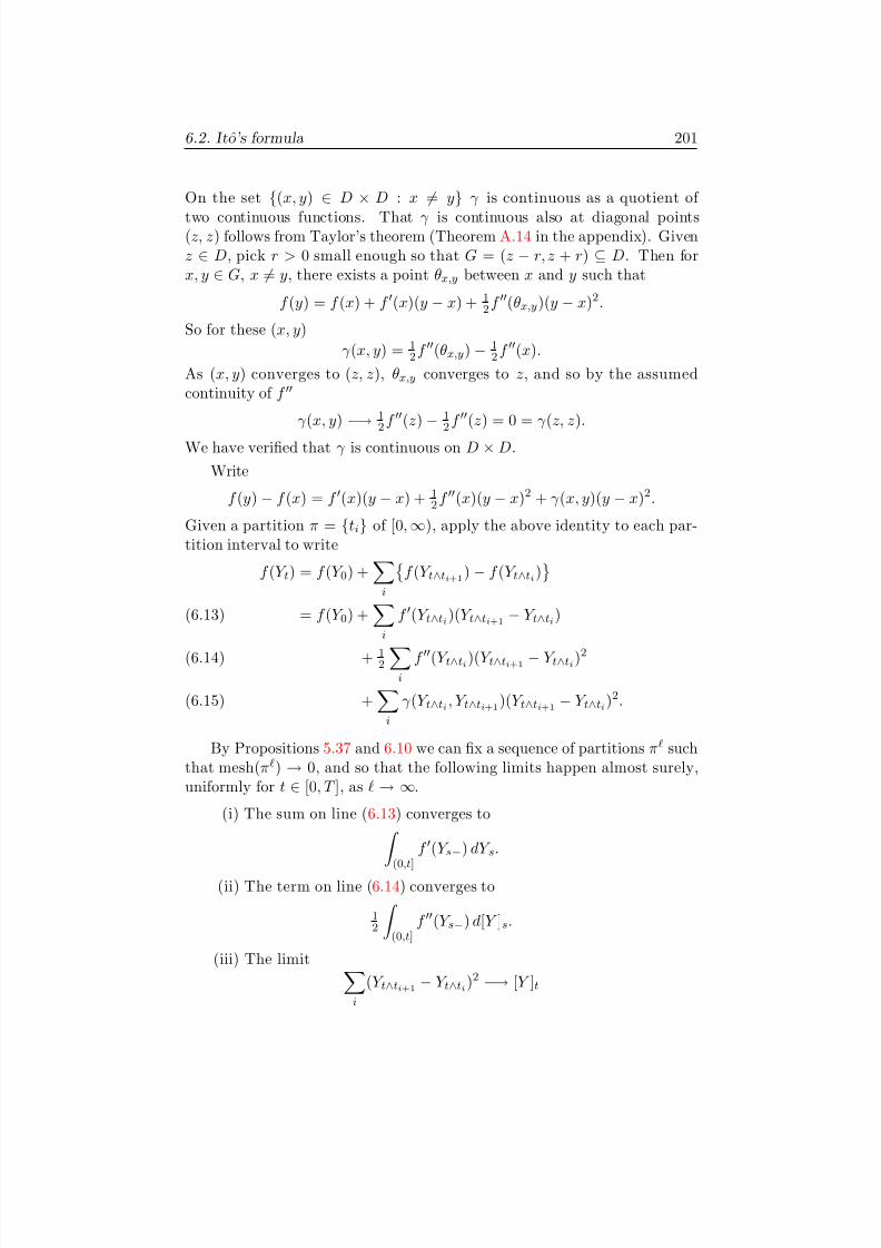
8/3/2019 Basics of Stochastic Analysis
http://slidepdf.com/reader/full/basics-of-stochastic-analysis 205/330
6.2. Itˆo’s formula 201
On the set (x, y ) ∈D ×D : x = y γ is continuous as a quotient of
two continuous functions. That γ is continuous also at diagonal points(z, z ) follows from Taylor’s theorem (Theorem A.14 in the appendix). Givenz∈D , pick r > 0 small enough so that G = ( z −r, z + r )⊆D . Then forx, y∈G, x = y, there exists a point θx,y between x and y such that
f (y) = f (x) + f (x)(y −x) + 12 f (θx,y )(y −x)2.
So for these (x, y)γ (x, y) = 1
2 f (θx,y ) − 12 f (x).
As (x, y) converges to ( z, z ), θx,y converges to z, and so by the assumedcontinuity of f
γ (x, y)
−→12 f (z)
−12 f (z) = 0 = γ (z, z ).
We have veried that γ is continuous on D ×D .Write
f (y) −f (x) = f (x)(y −x) + 12 f (x)(y −x)2 + γ (x, y)(y −x)2.
Given a partition π = t iof [0, ∞), apply the above identity to each par-tition interval to write
f (Y t ) = f (Y 0) +i
f (Y t∧t i +1 ) −f (Y t∧t i )
= f (Y 0) +i
f (Y t∧t i )(Y t∧t i +1 −Y t∧t i )(6.13)
+ 12i
f (Y t∧t i )(Y t∧t i +1 −Y t∧t i )2(6.14)
+i
γ (Y t∧t i , Y t∧t i +1 )(Y t∧t i +1 −Y t∧t i )2.(6.15)
By Propositions 5.37 and 6.10 we can x a sequence of partitions π suchthat mesh( π ) →0, and so that the following limits happen almost surely,uniformly for t∈[0, T ], as → ∞.
(i) The sum on line ( 6.13) converges to
(0,t ]
f (Y s−) dY s .
(ii) The term on line ( 6.14) converges to
12 (0,t ]
f (Y s−) d[Y ]s .
(iii) The limit
i(Y t∧t i +1 −Y t∧t i )
2 −→[Y ]t

8/3/2019 Basics of Stochastic Analysis
http://slidepdf.com/reader/full/basics-of-stochastic-analysis 206/330
202 6. It o’s Formula
happens.
Fix ω so that the limits in items (i)–(iii) above happen. We applythe scalar case of Lemma A.13, but simplied so that φ and γ in (A.8)have no time variables, to the cadlag function s →Y s (ω) on [0, t ] and thesequence of partitions π chosen above. For the closed set K in LemmaA.13 take K = Y [0, T ]. For the continuous function φ in Lemma A.13 takeφ(x, y) = γ (x, y)(y −x)2. By hypothesis, K is a subset of D . Consequently,as veried above, the function
γ (x, y ) =(x −y)−2φ(x, y), x = y0, x = y
is continuous on K
×K . Assumption ( A.9) of Lemma A.13 holds by item (iii)
above. The hypotheses of Lemma A.13 have been veried. The conclusionis that for this xed ω and each t∈[0, T ], the sum on line ( 6.15) convergesto
s∈(0 ,t ]
φ(Y s−, Y s ) =s∈(0,t ]
γ (Y s−, Y s ) Y s −Y s−2
=s∈(0 ,t ]
f (Y s ) −f (Y s−) −f (Y s−)∆ Y s − 12 f (Y s−)(∆ Y s )2 .
Lemma A.13 also contains the conclusion that this last sum is absolutelyconvergent.
To summarize, given 0 < T < ∞, we have shown that for almost everyω, (6.11) holds for all 0 ≤ t ≤T .
Remark 6.12. (Semimartingale property) A corollary of Theorem 6.11 isthat under the conditions of the theorem f (Y ) is a semimartingale. Equation(6.11) expresses f (Y ) as a sum of semimartingales. The integral f (Y −) d [Y ]is an FV process. To see that the sum over jump times s∈(0, t ] producesalso an FV process, x ω such that Y s (ω) is a cadlag function and ( 6.11)holds. Let s idenote the (at most countably many) jumps of s →Y s (ω)in [0, T ]. The theorem gives the absolute convergence
i
∆ f (Y s i (ω)) −f (Y s i −(ω))∆ Y s i (ω) − 12 f (Y s i −(ω))(∆ Y s i (ω)) 2 < ∞.
Consequently for this xed ω the sum in ( 6.11) denes a function in BV [0, T ],as in Example 1.14.
Let us state some simplications of Itˆ o’s formula.
Corollary 6.13. Under the hypotheses of Theorem 6.11 we have the follow-ing special cases.
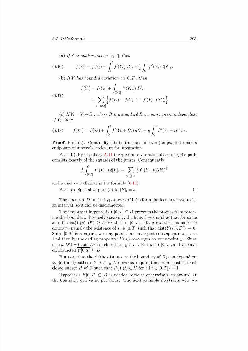
8/3/2019 Basics of Stochastic Analysis
http://slidepdf.com/reader/full/basics-of-stochastic-analysis 207/330
6.2. Itˆo’s formula 203
(a) If Y is continuous on [0, T ], then
(6.16) f (Y t ) = f (Y 0) + t
0f (Y s ) dY s + 1
2 t
0f (Y s ) d[Y ]s .
(b) If Y has bounded variation on [0, T ], then
f (Y t ) = f (Y 0) + (0 ,t ]f (Y s−) dY s
+s∈(0,t ]
f (Y s ) −f (Y s−) −f (Y s−)∆ Y s(6.17)
(c) If Y t = Y 0 + B t , where B is a standard Brownian motion independent of Y 0, then
(6.18) f (B t ) = f (Y 0) + t
0f (Y 0 + B s ) dB s + 1
2 t
0f (Y 0 + B s ) ds.
Proof. Part (a). Continuity eliminates the sum over jumps, and rendersendpoints of intervals irrelevant for integration.
Part (b). By Corollary A.11 the quadratic variation of a cadlag BV pathconsists exactly of the squares of the jumps. Consequently
12 (0,t ]
f (Y s−) d[Y ]s =s∈(0,t ]
12 f (Y s−)(∆ Y s )2
and we get cancellation in the formula ( 6.11).Part (c). Specialize part (a) to [ B ]t = t.
The open set D in the hypotheses of Itˆo’s formula does not have to bean interval, so it can be disconnected.
The important hypothesis Y [0, T ]⊆D prevents the process from reach-ing the boundary. Precisely speaking, the hypothesis implies that for someδ > 0, dist( Y (s), D c) ≥ δ for all s ∈[0, T ]. To prove this, assume thecontrary, namely the existence of s i ∈[0, T ] such that dist( Y (s i ), D c) →0.Since [0, T ] is compact, we may pass to a convergent subsequence s i →s.And then by the cadlag property, Y (s i ) converges to some point y. Since
dist( y, Dc) = 0 and D
cis a closed set, y
∈D
c. But y
∈Y [0, T ], and we havecontradicted Y [0, T ]⊆D .
But note that the δ (the distance to the boundary of D ) can depend onω. So the hypothesis Y [0, T ]⊆D does not require that there exists a xedclosed subset H of D such that P Y (t)∈H for all t∈[0, T ]= 1.
Hypothesis Y [0, T ] ⊆D is needed because otherwise a “blow-up” atthe boundary can cause problems. The next example illustrates why we
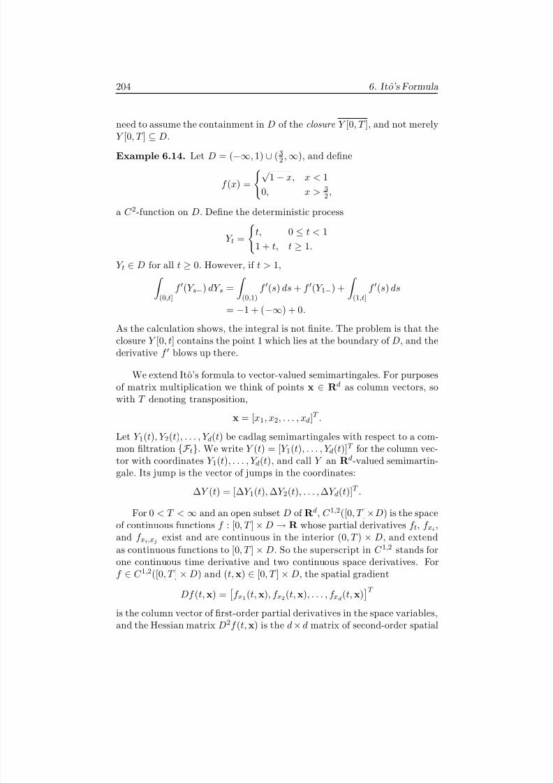
8/3/2019 Basics of Stochastic Analysis
http://slidepdf.com/reader/full/basics-of-stochastic-analysis 208/330
204 6. It o’s Formula
need to assume the containment in D of the closure Y [0, T ], and not merely
Y [0, T ]⊆
D .Example 6.14. Let D = ( −∞, 1)∪( 3
2 , ∞), and dene
f (x) =√1 −x, x < 10, x > 3
2 ,
a C 2-function on D . Dene the deterministic process
Y t =t, 0 ≤ t < 11 + t, t ≥1.
Y t
∈
D for all t
≥0. However, if t > 1,
(0,t ]f (Y s−) dY s = (0 ,1)
f (s) ds + f (Y 1−) + (1,t ]f (s) ds
= −1 + ( −∞) + 0 .
As the calculation shows, the integral is not nite. The problem is that theclosure Y [0, t ] contains the point 1 which lies at the boundary of D , and thederivative f blows up there.
We extend Itˆo’s formula to vector-valued semimartingales. For purposesof matrix multiplication we think of points x ∈R d as column vectors, sowith T denoting transposition,
x = [x1, x2, . . . , x d]T .
Let Y 1(t), Y 2(t), . . . , Y d(t) be cadlag semimartingales with respect to a com-mon ltration F t. We write Y (t) = [Y 1(t), . . . , Y d(t)]T for the column vec-tor with coordinates Y 1(t), . . . , Y d(t), and call Y an R d-valued semimartin-gale. Its jump is the vector of jumps in the coordinates:
∆ Y (t) = [∆ Y 1(t), ∆ Y 2(t), . . . , ∆ Y d(t)]T .
For 0 < T < ∞and an open subset D of R d , C 1,2([0, T ]×D ) is the spaceof continuous functions f : [0, T ]×D →R whose partial derivatives f t , f x i ,and f x i ,x j exist and are continuous in the interior (0 , T )
×D , and extend
as continuous functions to [0 , T ] ×D . So the superscript in C 1,2 stands forone continuous time derivative and two continuous space derivatives. Forf ∈C 1,2([0, T ]×D ) and ( t, x )∈[0, T ]×D, the spatial gradient
Df (t, x ) = f x1 (t, x ), f x2 (t, x ), . . . , f xd (t, x ) T
is the column vector of rst-order partial derivatives in the space variables,and the Hessian matrix D 2f (t, x ) is the d×d matrix of second-order spatial
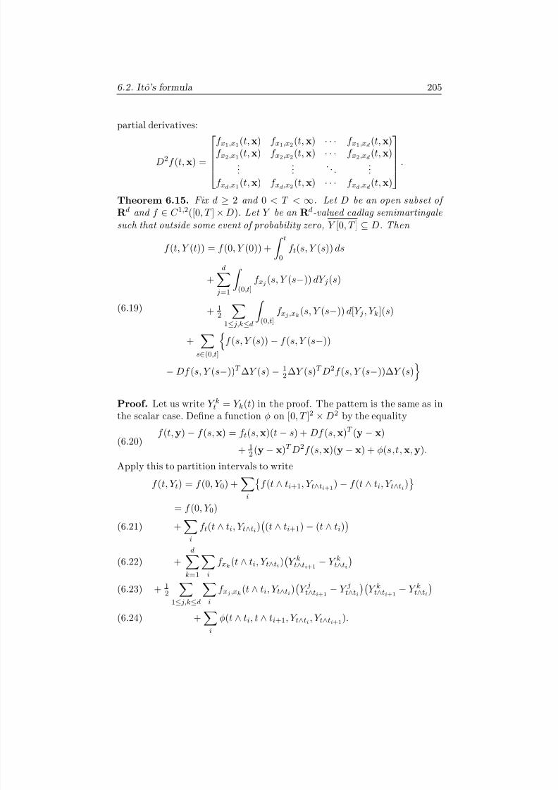
8/3/2019 Basics of Stochastic Analysis
http://slidepdf.com/reader/full/basics-of-stochastic-analysis 209/330
6.2. Itˆo’s formula 205
partial derivatives:
D 2f (t, x ) =
f x1 ,x 1 (t, x ) f x1 ,x 2 (t, x ) · · · f x1 ,x d (t, x )f x2 ,x 1 (t, x ) f x2 ,x 2 (t, x ) · · · f x2 ,x d (t, x )
...... . . . ...
f xd ,x 1 (t, x ) f xd ,x 2 (t, x ) · · · f xd ,x d (t, x )
.
Theorem 6.15. Fix d ≥ 2 and 0 < T < ∞. Let D be an open subset of R d and f ∈C 1,2([0, T ]×D ). Let Y be an R d-valued cadlag semimartingalesuch that outside some event of probability zero, Y [0, T ]⊆D . Then
f (t, Y (t)) = f (0, Y (0)) + t
0f t (s, Y (s)) ds
+d
j =1 (0 ,t ]f x j (s, Y (s−)) dY j (s)
+ 12
1≤ j,k ≤d (0 ,t ]f x j ,x k (s, Y (s−)) d[Y j , Y k ](s)
+s∈(0 ,t ]
f (s, Y (s)) −f (s, Y (s−))
−Df (s, Y (s−))T ∆ Y (s) − 12 ∆ Y (s)T D 2f (s, Y (s−))∆ Y (s)
(6.19)
Proof. Let us write Y kt = Y k (t) in the proof. The pattern is the same as inthe scalar case. Dene a function φ on [0, T ]2 ×D 2 by the equality
f (t, y ) −f (s, x ) = f t (s, x )( t −s) + Df (s, x )T (y −x )
+ 12 (y −x )T D 2f (s, x )(y −x ) + φ(s,t, x , y ).
(6.20)
Apply this to partition intervals to write
f (t, Y t ) = f (0, Y 0) +i
f (t∧t i+1 , Y t∧t i +1 ) −f (t∧t i , Y t∧t i )
= f (0, Y 0)
+i
f t (t∧t i , Y t∧t i ) (t∧t i+1 ) −(t∧t i )(6.21)
+ d
k=1 i
f xk (t∧t i , Y t∧t i ) Y kt∧t i +1 −Y kt∧t i(6.22)
+ 12
1≤ j,k ≤d i
f x j ,x k (t∧t i , Y t∧t i ) Y jt∧t i +1 −Y jt∧t i Y kt∧t i +1 −Y kt∧t i(6.23)
+i
φ(t∧t i , t∧t i+1 , Y t∧t i , Y t∧t i +1 ).(6.24)
8/3/2019 Basics of Stochastic Analysis
http://slidepdf.com/reader/full/basics-of-stochastic-analysis 210/330
206 6. It o’s Formula
By Propositions 5.37 and 6.10 we can x a sequence of partitions π such
that mesh( π ) →0, and so that the following limits happen almost surely,uniformly for t∈[0, T ], as → ∞.
(i) Line (6.21) converges to
(0,t ]f t (s, Y s ) ds.
(ii) Line (6.22) converges to
d
k=1 (0,t ]f xk (s, Y s−) dY ks .
(iii) Line (6.23) converges to
12
1≤ j,k ≤d (0 ,t ]f x j ,x k (s, Y s−) d[Y j , Y k ]s .
(iv) The limit
i
Y kt∧t i +1 −Y kt∧t i
2
−→[Y k]t
happens for 1 ≤k ≤d.
Fix ω such that Y [0, T ]
⊆
D and the limits in items (i)–(iv) hold. By the
above paragraph and by hypothesis these conditions hold for almost everyω.
To treat the sum on line ( 6.24), we apply Lemma A.13 to the R d-valuedcadlag function s →Y s (ω) on [0, T ], with the function φ dened by ( 6.20),the closed set K = Y [0, T ], and the sequence of partitions π chosen above.We need to check that φ and the set K satisfy the hypotheses of LemmaA.13. Continuity of φ follows from the denition ( 6.20). Next we argue thatif (sn , tn , x n , y n ) →(u,u, z , z ) in [0, T ]2 ×K 2 while for each n, either sn = tnor x n = y n , then
(6.25)φ(sn , tn , x n , y n )
|tn −
sn |
+
|y
n −x
n |2 →0.
Given ε > 0, let I be an interval around u in [0, T ] and let B be an openball centered at z and contained in D such that
|f t (v, w ) −f t (u, z )|+ |D 2f (v, w ) −D 2f (u, z )| ≤ε
for all v∈I, w ∈B . Such an interval I and ball B exist by the openness of D and by the assumption of continuity of derivatives of f in [0, T ]×D . For

8/3/2019 Basics of Stochastic Analysis
http://slidepdf.com/reader/full/basics-of-stochastic-analysis 211/330
6.2. Itˆo’s formula 207
large enough n, we have sn , tn ∈I and x n , y n ∈B . Since a ball is convex,
by Taylor’s formula ( A.16) we can writeφ(sn , tn , x n , y n ) = f t (τ n , y n ) −f t (sn , x n ) (tn −sn )
+ 12 (y n −x n )T D 2f (sn , ξn ) −D 2f (sn , x n ) (y n −x n ),
where τ n lies between sn and tn , and ξn is a point on the line segmentconnecting x n and y n . Hence τ n ∈I and ξn ∈B , and by Schwarz inequalityin the form ( A.7),
|φ(sn , tn , x n , y n )| ≤ f t (τ n , y n ) −f t (sn , x n ) · |tn −sn |+ D 2f (sn , ξn ) −D 2f (tn , x n ) · |y n −x n |2
≤2ε · |tn −sn |+ |y n −x n |2 .
Thusφ(sn , tn , x n , y n )
|tn −sn |+ |y n −x n |2 ≤2ε
for large enough n, and we have veried ( 6.25).The function
(s,t, x , y ) →φ(s,t, x , y )
|t −s|+ |y −x |2is continuous at points where either s = t or x = y , as a quotient of twocontinuous functions. Consequently the function γ dened by ( A.8) is con-tinuous on [0 , T ]2 ×K 2.
Hypothesis ( A.9) of Lemma A.13 is a consequence of the limit in item(iv) above.
The hypotheses of Lemma A.13 have been veried. By this lemma, forthis xed ω and each t∈[0, T ], the sum on line (6.24) converges to
s∈(0,t ]
φ(s,s,Y s−, Y s ) =s∈(0 ,t ]
f (s, Y s ) −f (s, Y s−)
−Df (s, Y s−)∆ Y s − 12 ∆ Y T
s D 2f (s, Y s−)∆ Y s .
This completes the proof of Theorem 6.15.
Remark 6.16. (Notation) Often Itˆ o’s formula is expressed in terms of dif-ferential notation which is more economical than the integral notation. Asan example, if Y is a continuous R d-valued semimartingale, equation ( 6.19)can be written as
df (t, Y (t)) = f t (t, Y (t)) dt +d
j =1
f x j (t, Y (t−)) dY j (t)
+ 12
1≤ j,k ≤d
f x j ,x k (t, Y (t−)) d[Y j , Y k ](t).(6.26)
8/3/2019 Basics of Stochastic Analysis
http://slidepdf.com/reader/full/basics-of-stochastic-analysis 212/330
208 6. It o’s Formula
As mentioned already, these “stochastic differentials” have no rigorous mean-
ing. The formula above is to be regarded only as an abbreviation of theintegral formula ( 6.19).
We state the Brownian motion case as a corollary. For f ∈C 2(D ) inR d , the Laplace operator ∆ is dened by
∆ f = f x1 ,x 1 + · · ·+ f xd ,x d .
A function f is harmonic in D if ∆ f = 0 on D .
Corollary 6.17. Let B (t) = ( B1(t), . . . , B d(t)) be Brownian motion in R d,with random initial point B (0) , and f ∈C 2(R d). Then
(6.27) f (B (t)) = f (B (0)) + t
0 Df (B (s))T
dB (s) +12
t
0 ∆ f (B (s)) ds.
Suppose f is harmonic in an open set D⊆R d . Let D1 be an open subset of D such that dist( D1, D c) > 0. Assume initially B (0) = z for some point z∈D1, and let
(6.28) τ = inf t ≥0 : B (t)∈D c1
be the exit time for Brownian motion from D1. Then f (B τ (t)) is a local L2-martingale.
Proof. Formula ( 6.27) comes directly from Itˆo’s formula, because [ B i , B j ] =δi,j t .
The process B τ is a (vector) L2 martingale that satises B τ [0, T ]⊆
Dfor all T < ∞. Thus Itˆo’s formula applies. Note that [ B τ
i , B τ j ] = [B i , B j ]τ =
δi,j (t∧τ ). Hence ∆ f = 0 in D eliminates the second-order term, and theformula simplies to
f (B τ (t)) = f (z ) + t
0Df (B τ (s))T dB τ (s)
which shows that f (B τ (t)) is a local L2-martingale.
6.3. Applications of Itˆ o’s formula
One can use It o’s formula to nd pathwise expressions for stochastic inte-grals.
Example 6.18. To evaluate t0 B k
s dB s for standard Brownian motion andk ≥ 1, take f (x) = ( k + 1) −1xk+1 , so that f (x) = xk and f (x) = kx k−1.It o’s formula gives
t
0B k
s dB s = ( k + 1) −1B k+1t −
k2 t
0B k−1
s ds.
8/3/2019 Basics of Stochastic Analysis
http://slidepdf.com/reader/full/basics-of-stochastic-analysis 213/330
6.3. Applications of Itˆ o’s formula 209
The integral on the right is a familiar Riemann integral of the continuous
function s →B k−1s .
One can use Itˆo’s formula to nd martingales, which in turn are usefulfor calculations, as the next lemma and example show.
Lemma 6.19. Suppose f ∈C 1,2(R + ×R ) and f t + 12 f xx = 0 . Let B t be
one-dimensional standard Brownian motion. Then f (t, B t ) is a local L2-martingale. If
(6.29) T
0E f x (t, B t )2 dt < ∞,
then f (t, B t ) is an L2-martingale on [0, T ].
Proof. Since [B ]t = t, (6.19) specializes to
f (t, B t ) = f (0, 0) + t
0f x (s, B s ) dB s + t
0f t (s, B s ) + 1
2 f xx (s, B s ) ds
= f (0, 0) + t
0f x (s, B s ) dB s
where the last line is a local L2-martingale. (The integrand f x (s, B s ) is acontinuous process, hence predictable, and satises the local boundednesscondition ( 5.29).)
The integrability condition ( 6.29) guarantees that f x(s, B
s) lies in the
space L2(B, P ) of integrands on the interval [0 , T ]. In our earlier develop-ment of stochastic integration we always considered processes dened for alltime. To get an integrand process on the entire time line [0 , ∞), one canextend f x (s, B s ) by declaring it identically zero on ( T,∞). This does notchange the integral on [0 , T ].
Example 6.20. Let µ∈R and σ = 0 be constants. Let a < 0 < b. LetB t be one-dimensional standard Brownian motion, and X t = µt + σB t aBrownian motion with drift. Question: What is the probability that X texits the interval ( a, b) through the point b?
Dene the stopping time
τ = inf t > 0 : B t = a or B t = b.
First we need to check that τ < ∞almost surely. For example, the events
σB n +1 −σB n > b −a + |µ|+ 1, n = 0 , 1, 2, . . .
are independent and have a common positive probability. Hence one of themhappens almost surely. Consequently X n cannot remain in ( a, b) for all n.

8/3/2019 Basics of Stochastic Analysis
http://slidepdf.com/reader/full/basics-of-stochastic-analysis 214/330
210 6. It o’s Formula
We seek a function h such that h(X t ) is a martingale. Then, if we could
justify Eh (X τ ) = h(0), we could compute the desired probability P (X τ = b)from
h(0) = Eh (X τ ) = h(a)P (X τ = a) + h(b)P (X τ = b).
To utilize Lemma 6.19, let f (t, x ) = h(µt + σx ). The condition f t + 12 f xx = 0
becomesµh + 1
2 σ2h = 0 .
At this point we need to decide whether µ = 0 or not. Let us work the caseµ = 0. Solving for h gives
h(x) = C 1 exp 2µσ−2x + C 2
for two constants of integration C 1, C 2. To check (6.29), from f (t, x ) =h(µt + σx ) derive
f x (t, x ) = −2C 2µσ−1 exp 2µσ−2(µt + σx) .
Since B t is a mean zero normal with variance t, one can verify that ( 6.29)holds for all T < ∞.
Now M t = h(X t ) is a martingale. By optional stopping, M τ ∧t is also amartingale, and so EM τ ∧t = EM 0 = h(0). By path continuity and τ < ∞,M τ ∧t →M τ almost surely as t → ∞. Furthermore, the process M τ ∧t isbounded, because up to time τ process X t remains in [ a, b], and so |M τ ∧t | ≤C
≡sup a
≤x
≤b
|h(x)
|. Dominated convergence gives EM τ
∧
t
→EM τ as t
→∞. We have veried that Eh (X τ ) = h(0).Finally, we can choose the constants C 1 and C 2 so that h(b) = 1 and
h(a) = 0. After some details,
(6.30) P (X τ = b) = h(0) =e−2µa/σ 2
−1e−2µa/σ 2
−e−2µb/σ 2 .
Can you explain what you see as you let either a → −∞or b → ∞? (Deciderst whether µ is positive or negative.)
We leave the case µ = 0 as an exercise. You should get P (X τ = b) =(−a)/ (b−a).
Next we use It o’s formula to investigate recurrence and transience of Brownian motion, and whether Brownian motion ever hits a point. Let usrst settle these questions in one dimension.
Proposition 6.21. Let B t be Brownian motion in R . Then limt→∞B t = ∞and limt→∞B t = −∞, almost surely. Consequently almost every Brownian path visits every point innitely often.

8/3/2019 Basics of Stochastic Analysis
http://slidepdf.com/reader/full/basics-of-stochastic-analysis 215/330
6.3. Applications of Itˆ o’s formula 211
Proof. Let τ 0 = 0 and τ (k + 1) = inf t > τ (k) : |B t −Bτ (k)| = 4 k+1 . By
the strong Markov property of Brownian motion, for each k the restartedprocess Bτ (k)+ s −Bτ (k) : s ≥is a standard Brownian motion, independentof F τ (k) . Consequently, by the case µ = 0 of Example 6.20,
P Bτ (k+1) −Bτ (k) = 4 k+1 = P Bτ (k+1) −Bτ (k) = −4k+1 = 12 .
By the strong Markov property these random variables indexed by k areindependent. Thus, for almost every ω, there are arbitrarily large j and ksuch that Bτ ( j +1) −Bτ ( j ) = 4 j +1 and Bτ (k+1) −Bτ (k) = −4k+1 . But thensince
|Bτ ( j )| ≤ j
i=1
4i =4 j +1 −1
4
−1 ≤
4 j +1
2,
Bτ ( j +1) ≥4 j , and by the same argument Bτ (k+1) ≤ −4k . Thus lim t→∞B t =
∞and lim t→∞B t = −∞almost surely.Almost every Brownian path visits every point innitely often due to a
special property of one dimension: it is impossible to go “around” a point.
Proposition 6.22. Let B t be Brownian motion in R d , and let P z denotethe probability measure when the process B t is started at point z∈R d . Let
τ r = inf t ≥0 : |B t | ≤rbe the rst time Brownian motion hits the ball of radius r around the origin.
(a) If d = 2 , P z (τ r < ∞) = 1 for all r > 0 and z∈R d .(b) If d ≥3, then for z outside the ball of radius r ,
P z (τ r < ∞) =r
|z|d−2
.
There will be an almost surely nite time T such that |B t | > r for all t ≥T .(c) For d ≥2 and any z , y ∈R d ,
P z [ B t = y for all 0 < t < ∞] = 1.
Note that z = y is allowed. That is why t = 0 is not included in the event.
Proof. Observe that for (c) it suffices to consider y = 0, because
P z [ B t = y for all 0 < t < ∞] = P z−y [ B t = 0 for all 0 < t < ∞].
Then, it suffices to consider z = 0, because if we have the result for all z = 0,then we can use the Markov property to restart the Brownian motion after
8/3/2019 Basics of Stochastic Analysis
http://slidepdf.com/reader/full/basics-of-stochastic-analysis 216/330
212 6. It o’s Formula
a small time s:
P 0[ B t = 0 for all 0 < t < ∞]
= lims 0
P 0[ B t = 0 for all s < t < ∞]
= lims 0
E 0 P B (s)B t = 0 for all 0 < t < ∞= 1 .
The last equality is true because B (s) = 0 with probability one.Now we turn to the actual proofs, and we can assume z = 0 and the
small radius r < |z|.We start with dimension d = 2. The function g(x ) = log |x | is harmonic
in D = R 2
\ 0
. (Only in d = 2, check.) Let
σR = inf t ≥0 : |B t | ≥Rbe the rst time to exit the open ball of radius R. Pick r < |z| < R , anddene the annulus A = x : r < |x | < R . The time to exit the annulus isζ = τ r ∧σR . Since any coordinate of B t has limsup ∞almost surely, or bythe independent increments argument used in Example 6.20, the exit timeσR and hence also ζ is nite almost surely.
Apply Corollary 6.17 to the harmonic function
f (x ) =log R −log|x |log R −log r
and the annulus A. We get that f (Bζ ∧t ) is a local L2-martingale, and sincef is bounded on the closure of A, it follows that f (Bζ ∧t ) is an L2-martingale.The optional stopping argument used in Example 6.20, in conjunction withletting t → ∞, gives again f (z ) = E z f (B0) = E z f (Bζ ). Since f = 1 on theboundary of radius r but vanishes at radius R,
P z (τ r < σ R ) = P z ( |Bζ | = r ) = E z f (Bζ ) = f (z ),
and so
(6.31) P z (τ r < σ R ) =log R −log|z|log R −log r
.
From this we can extract both part (a) and part (c) for d = 2. First,σR ∞as R ∞because a xed path of Brownian motion is boundedon bounded time intervals. Consequently
P z (τ r < ∞) = limR→∞
P z (τ r < σ R )
= limR→∞
log R −log|z|log R −log r
= 1 .
8/3/2019 Basics of Stochastic Analysis
http://slidepdf.com/reader/full/basics-of-stochastic-analysis 217/330
6.3. Applications of Itˆ o’s formula 213
Secondly, consider r = r (k) = (1 /k )k and R = R(k) = k. Then we get
P z (τ r (k) < σ R (k) ) =log k −log|z|(k + 1) log k
which vanishes as k → ∞. Let τ = inf t ≥0 : B t = 0be the rst hittingtime of 0. For r < |z|, τ r ≤ τ because B t cannot hit zero without rstentering the ball of radius r . Again since σR (k) ∞as k ∞,
P z (τ < ∞) = limk→∞
P z (τ < σ R (k) )
≤ limk→∞
P z (τ r (k) < σ R (k) ) = 0 .
For dimension d ≥ 3 we use the harmonic function g(x ) = |x |2−d , and
apply Itˆo’s formula to the function
f (x ) =R2−d − |x |2−d
R2−d −r 2−d .
The annulus A and stopping times σR and ζ are dened as above. The samereasoning now leads to
(6.32) P z (τ r < σ R ) =R2−d − |z|2−d
R2−d −r 2−d .
Letting R → ∞gives
P z (τ r < ∞) = |z|2−d
r 2
−d =
r
|z
|
d−2
as claimed. Part (c) follows now because the quantity above tends to zeroas r →0.
It remains to show that after some nite time, the ball of radius r is nolonger visited. Let r < R . Dene σ1
R = σR , and for n ≥2,
τ nr = inf t > σ n−1R : |B t | ≤r
andσn
R = inf t > τ nr : |B t | ≥R.
In other words, σ1R < τ 2
r < σ 2R < τ 3
r < · · ·are the successive visits to radiusR and back to radius r . Let α = ( r/R )d−2 < 1. We claim that for n
≥2,
P z (τ nr < ∞) = αn−1.
For n = 2, since σ1R < τ 2
r , use the strong Markov property to restart theBrownian motion at time σ1
R .
P z (τ 2r < ∞) = P z (σ1R < τ 2
r < ∞)
= E z P B (σ1R )τ r < ∞= α.
8/3/2019 Basics of Stochastic Analysis
http://slidepdf.com/reader/full/basics-of-stochastic-analysis 218/330
214 6. It o’s Formula
Then by induction.
P z (τ nr < ∞) = P z (τ n−1r < σ n−1
R < τ nr < ∞)
= E z 1τ n−1r < σ n−1
R < ∞P B (σn − 1R )τ r < ∞
= P z (τ n−1r < ∞) ·α = α n−1.
Above we used the fact that if τ n−1r < ∞, then necessarily σn−1
R < ∞because each coordinate of B t has limsup ∞.The claim implies
nP z (τ nr < ∞) < ∞.
By Borel-Cantelli, τ nr <
∞can happen only nitely many times, almost
surely.
Remark 6.23. We see here an example of an uncountable family of eventswith probability one whose intersection must vanish. Namely, the inter-section of the events that Brownian motion does not hit a particular pointwould be the event that Brownian motion never hits any point. Yet Brow-nian motion must reside somewhere.
Theorem 6.24. (Levy’s Characterization of Brownian Motion.) Let M =[M 1, . . . , M d]T be a continuous R d-valued local martingale with M (0) = 0 .Then M is a standard Brownian motion iff [M i , M j ]t = δi,j t .
Proof. We already know that a d-dimensional standard Brownian motionsatises [B i , B j ]t = δi,j t .
What we need to show is that M with the assumed covariance is Brow-nian motion. As a continuous local martingale, M is also a local L2-martingale. Fix a vector θ = ( θ1, . . . , θd)T
∈R d and
f (t, x ) = exp( iθT x + 12 |θ|2t).
Let Z t = f (t, M (t)). It o’s formula applies equally well to complex-valuedfunctions, and so
Z t = 1 + |θ|22
t
0
Z s ds +d
j =1
iθ j
t
0
Z s dM j (s)
−12
d
j =1θ2 j t
0Z s ds
= 1 +d
j =1
iθ j t
0Z s dM j (s).

8/3/2019 Basics of Stochastic Analysis
http://slidepdf.com/reader/full/basics-of-stochastic-analysis 219/330
8/3/2019 Basics of Stochastic Analysis
http://slidepdf.com/reader/full/basics-of-stochastic-analysis 220/330
216 6. It o’s Formula
Rearranging the above inequality gives the conclusion for a bounded mar-
tingale. The constant C p changes along the way but depends only on p.The general case comes by localization. Let τ k = inf t ≥0 : |M t | ≥k,
a stopping time by Corollary 2.10. By continuity M τ k is bounded, so wecan apply the already proved result to claim
E [(M ∗τ k∧t ) p] ≤C pE [M ] p/ 2
τ k∧t .
On both sides monotone convergence leads to ( 6.33) as k ∞.
Exercises
Exercise 6.1. Does part (a) of Lemma 6.4 extend to semimartingales?
Exercise 6.2. (a) Let Y be a cadlag semimartingale with Y 0 = 0. Checkthat Itˆo’s formula gives 2 Y −dY = Y 2 + [ Y ], as already follows from theintregration by parts formula ( 6.7).
(b) Let N be a rate α Poisson process and M t = N t −αt . Apply part(a) to show that M 2t −N t is a martingale.
Exercise 6.3. Let B t be standard Brownian motion and M t = B 2t −t .
(a) Justify the identity [ M ] = [B 2]. (Use the linearity ( 6.4).)(b) Apply Itˆo’s formula to B 2
t and from that nd a representation for[B 2] in terms of a single ds-integal.
(c) Using It o’s formula and your answer to (b), check that M 2
−[B 2]
is a martingale, as it should. (Of course without appealing to the fact thatM 2 −[B 2] = M 2 −[M ] is a martingale.)
(d) Use integration by parts ( 6.7) to nd another representation of [ B 2].Then use Itˆo’s formula to show that this representation agrees with theanswer in (b).
Exercise 6.4. (a) Check that for a rate α Poisson process N It o’s formulareduces to an obvious identity, namely a telescoping sum over jumps thatcan be written as
(6.34) f (N t ) = f (0) +
(0 ,t ]
f (N s ) −f (N s−) dN s .
(b) Suppose E T 0 |f (N s )|2 ds < ∞. Show that for t∈[0, T ]
(6.35) E [f (N t )] = f (0) + E t
0f (N s + 1) −f (N s ) αds.
Warning. Do not attempt to apply stochastic calculus to non-predictableintegrands.

8/3/2019 Basics of Stochastic Analysis
http://slidepdf.com/reader/full/basics-of-stochastic-analysis 221/330
Exercises 217
Exercise 6.5. Suppose X is a nondecreasing cadlag process such that
X (0) = 0, all jumps are of size 1 (that is, X s −X s− = 0 or 1), between jumps X is constant, and M t = X t −αt is a martingale. Show that X is arate α Poisson process. Hint. Imitate the proof of Theorem 6.24.
Exercise 6.6. Let B be standard one-dimensional Brownian motion. Showthat for a continuously differentiable nonrandom function φ,
t
0φ(s) dB s = φ(t)B t − t
0B s φ (s) ds.
Exercise 6.7. Dene
V 1(t) = t
0B s ds, V 2(t) =
t
0V 1(s) ds,
and generally
V n (t) = t
0V n−1(s) ds = t
0ds1 s1
0ds2 · · · sn − 1
0dsn B sn .
V n is known as n times integrated Brownian motion, and appears in appli-cations in statistics. Show that
V n (t) =1n! t
0(t −s)n dB s .
Then show that the process
M n (t) = V n (t) −n
j =1
t j j !(n − j )!
t
0(−s)n− j dB s
is a martingale.
Exercise 6.8. Let X and Y be independent rate α Poisson processes.
(a) Show that
P X and Y have no jumps in common = 1 .
Find the covariation [ X, Y ].
(b) Find a process U such that X t Y t −U t is a martingale.
Exercise 6.9. Let D = R 3\0, the complement of the origin in R 3. Denef ∈C 2(D) by
f (x ) =1
|x |=
1(x2
1 + x22 + x2
3)1/ 2
Let B (t) = ( B1(t), B2(t), B3(t)) be Brownian motion in R 3 started at somepoint B (0) = z = 0. Show that f (B t ) is a uniformly integrable local L2-martingale, but not a martingale.

8/3/2019 Basics of Stochastic Analysis
http://slidepdf.com/reader/full/basics-of-stochastic-analysis 222/330
218 6. It o’s Formula
The point of the exercise is that a bounded local martingale is a martin-
gale, so it is natural to ask whether a uniformly integrable local martingaleis a martingale.
Hints. From Proposition 6.22 P z B t = 0 for all t= 1. Uniform inte-grability follows for example from having E [f (B t )2] bounded in t. A mar-tingale has a constant expectation.
Exercise 6.10. Let B t be Brownian motion in R k started at point z∈R k .As before, let
σR = inf t ≥0 : |B t | ≥Rbe the rst time the Brownian motion leaves the ball of radius R. Computethe expectation E z [σR ] as a function of z , k and R.
Hint. Start by applying Itˆ o’s formula to f (x ) = x21 + · · ·+ x
2k .
Exercise 6.11. Provide the proof for Remark 6.25.
Exercise 6.12. (Space-time Poisson random measure) In some applicationsthe random occurrences modeled by a Poisson process also come with aspatial structure. Let U be a subset of R d and ν a nite Borel measureon U . Let ξ be a Poisson random measure on U ×R + with mean measureν ⊗m. Dene the ltration F t = σξ(B ) : B ∈ BU ×[0,t ]. Fix a boundedBorel function h on U ×R + . Dene
X t =
U
×[0,t ]
h(x, s ) ξ(dx, ds ) , H t =
t
0
U
h(x, s ) ν (dx) ds
and M t = X t −H t .(a) Show that these are cadlag processes, M is a martingale, H is an FV
process and X is semimartingale.(b) Show that for an adapted cadlag process Z ,
(0 ,t ]Z (s−) dX s = U ×[0,t ]
Z (s−)h(x, s ) ξ(dx, ds ).
Hint. The Riemann sums in Proposition 5.37 would work.(c) Show that for an adapted cadlag process Z ,
E
(0 ,t ]
Z (s
−) dX s =
t
0
U
E [Z (s)]h(x, s ) ν (dx) ds.
What moment assumptions to do you need for Z ?

8/3/2019 Basics of Stochastic Analysis
http://slidepdf.com/reader/full/basics-of-stochastic-analysis 223/330
Chapter 7
Stochastic DifferentialEquations
In this chapter we study equations of the type
(7.1) X (t, ω) = H (t, ω) + (0,t ]F (s ,ω,X (ω)) dY (s, ω)
for an unknown R d-valued process X . In the equation, Y is a given R m -valued cadlag semimartingale and H is a given R d-valued adapted cadlagprocess. The coefficient F (t ,ω,η) is a d ×m-matrix valued function of thetime variable t , the sample point ω, and a cadlag path η. The integral
F dY with a matrix-valued integrand and vector-valued integrator has anatural componentwise interpretation, as explained in Remark 5.38.
Underlying the equation is a probability space (Ω , F , P ) with a ltration
F t, on which the ingredients H , Y and F are dened. A solution X isan R d-valued cadlag process that is dened on this given probability space(Ω, F , P ) and adapted to F t, and that satises the equation in the sensethat the two sides of ( 7.1) are indistinguishable. This notion is the so-calledstrong solution which means that the solution process can be constructedon the given probability space, adapted to the given ltration.
In order for the integral
F dY to be sensible, F has to have the prop-
erty that, whenever an adapted cadlag process X is substituted for η, theresulting process ( t, ω) →F (t ,ω,X (ω)) is predictable and locally boundedin the sense ( 5.36). We list precise assumptions on F when we state andprove an existence and uniqueness theorem.
Since the integral term vanishes at time zero, equation ( 7.1) containsthe initial value X (0) = H (0). The integral equation ( 7.1) can be written
219
8/3/2019 Basics of Stochastic Analysis
http://slidepdf.com/reader/full/basics-of-stochastic-analysis 224/330
220 7. Stochastic Differential Equations
in the differential form
(7.2) dX (t) = dH (t) + F (t, X ) dY (t), X (0) = H (0)
where the initial value must then be displayed explicitly. The notation canbe further simplied by dropping the superuous time variables:
(7.3) dX = dH + F (t, X ) dY, X (0) = H (0) .
Equations ( 7.2) and ( 7.3) have no other interpretation except as abbre-viations for ( 7.1). Equations such as ( 7.3) are known as SDE’s (stochasticdifferential equations) even though precisely speaking they are integral equa-tions.
7.1. Examples of stochastic equations and solutions
7.1.1. Itˆ o equations. Let B t be a standard Brownian motion in R m withrespect to a ltration F t. Let ξ be an R d-valued F 0-measurable ran-dom variable. Often ξ is a nonrandom point x0. The assumption of F 0-measurability implies that ξ is independent of the Brownian motion. An Itˆ oequation has the form
(7.4) dX t = b(t, X t ) dt + σ(t, X t ) dB t , X 0 = ξ
or in integral form
(7.5) X t = ξ + t
0b(s, X s ) ds +
t
0σ(s, X s ) dB s .
The coefficients b(t, x ) and σ(t, x ) are Borel measurable functions of ( t, x )∈[0, ∞) ×R d . The drift vector b(t, x ) is R d-valued, and the dispersion matrix σ(t, x ) is d ×m-matrix valued. The d ×d matrix a(t, x ) = σ(t, x )σ(t, x )T iscalled the diffusion matrix . X is the unknown R d-valued process.
Linear Itˆo equations can be explicitly solved by a technique from basictheory of ODEs (ordinary differential equations) known as the integrating factor . We begin with the nonrandom case from elementary calculus.
Example 7.1. (Integrating factor for linear ODEs.) Let a(t) and g(t) begiven functions. Suppose we wish to solve
(7.6) x + a(t)x = g(t)
for an unknown function x = x(t). The trick is to multiply through theequation by the integrating factor
(7.7) z(t) = eR t0 a(s) ds
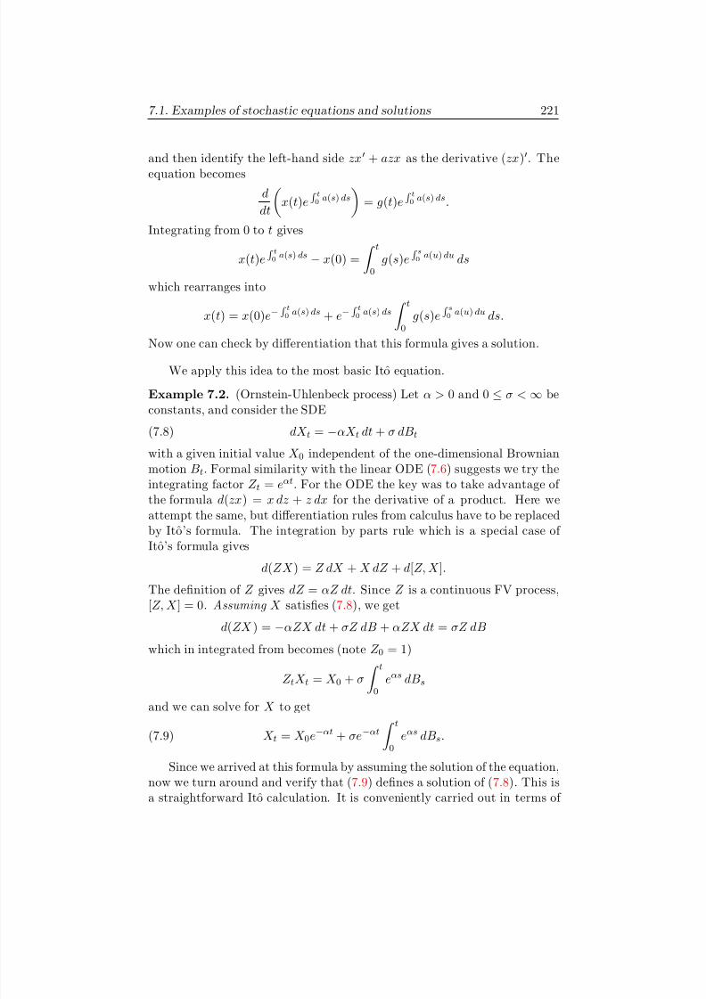
8/3/2019 Basics of Stochastic Analysis
http://slidepdf.com/reader/full/basics-of-stochastic-analysis 225/330
7.1. Examples of stochastic equations and solutions 221
and then identify the left-hand side zx + azx as the derivative ( zx ) . The
equation becomesddt
x(t)e R t0 a(s) ds = g(t)e R t
0 a(s) ds .
Integrating from 0 to t gives
x(t)e R t0 a(s) ds −x(0) = t
0g(s)e R s
0 a(u) du ds
which rearranges into
x(t) = x(0)e−R t0 a(s) ds + e−R t
0 a(s) ds t
0g(s)e R s
0 a(u) du ds.
Now one can check by differentiation that this formula gives a solution.We apply this idea to the most basic Itˆ o equation.
Example 7.2. (Ornstein-Uhlenbeck process) Let α > 0 and 0 ≤σ < ∞beconstants, and consider the SDE
(7.8) dX t = −αX t dt + σ dB t
with a given initial value X 0 independent of the one-dimensional Brownianmotion B t . Formal similarity with the linear ODE ( 7.6) suggests we try theintegrating factor Z t = eαt . For the ODE the key was to take advantage of the formula d(zx ) = x dz + z dx for the derivative of a product. Here weattempt the same, but differentiation rules from calculus have to be replacedby It o’s formula. The integration by parts rule which is a special case of It o’s formula gives
d(ZX ) = Z dX + X dZ + d[Z, X ].
The denition of Z gives dZ = αZ dt . Since Z is a continuous FV process,[Z, X ] = 0. Assuming X satises ( 7.8), we get
d(ZX ) = −αZX dt + σZ dB + αZX dt = σZ dB
which in integrated from becomes (note Z 0 = 1)
Z t X t = X 0 + σ
t
0eαs dB s
and we can solve for X to get
(7.9) X t = X 0e−αt + σe−αt t
0eαs dB s .
Since we arrived at this formula by assuming the solution of the equation,now we turn around and verify that ( 7.9) denes a solution of ( 7.8). This isa straightforward Itˆ o calculation. It is conveniently carried out in terms of
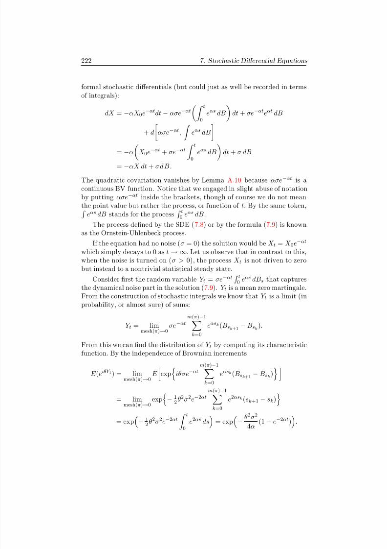
8/3/2019 Basics of Stochastic Analysis
http://slidepdf.com/reader/full/basics-of-stochastic-analysis 226/330
222 7. Stochastic Differential Equations
formal stochastic differentials (but could just as well be recorded in terms
of integrals):
dX = −αX 0e−αt dt −ασe −αt t
0eαs dB dt + σe−αt eαt dB
+ d ασe −αt , eαs dB
= −α X 0e−αt + σe−αt t
0eαs dB dt + σ dB
= −αX dt + σdB.
The quadratic covariation vanishes by Lemma A.10 because ασe −αt is a
continuous BV function. Notice that we engaged in slight abuse of notationby putting ασe −αt inside the brackets, though of course we do not meanthe point value but rather the process, or function of t. By the same token,
eαs dB stands for the process t0 eαs dB .
The process dened by the SDE ( 7.8) or by the formula ( 7.9) is knownas the Ornstein-Uhlenbeck process.
If the equation had no noise ( σ = 0) the solution would be X t = X 0e−αt
which simply decays to 0 as t → ∞. Let us observe that in contrast to this,when the noise is turned on ( σ > 0), the process X t is not driven to zerobut instead to a nontrivial statistical steady state.
Consider rst the random variable Y t = σe−αt
t
0 eαs dB s that captures
the dynamical noise part in the solution ( 7.9). Y t is a mean zero martingale.From the construction of stochastic integrals we know that Y t is a limit (inprobability, or almost sure) of sums:
Y t = limmesh( π )→0
σe−αtm (π )−1
k=0
eαs k (B sk +1 −B sk ).
From this we can nd the distribution of Y t by computing its characteristicfunction. By the independence of Brownian increments
E (eiθY t ) = limmesh( π )
→0
E exp iθσe−αtm (π )−1
k=0
eαs k (B sk +1 −B sk )
= limmesh( π )→0
exp −12 θ2σ2e−2αt
m (π )−1
k=0
e2αs k (sk+1 −sk)
= exp −12 θ2σ2e−2αt t
0e2αs ds = exp −
θ2σ2
4α(1 −e−2αt ) .

8/3/2019 Basics of Stochastic Analysis
http://slidepdf.com/reader/full/basics-of-stochastic-analysis 227/330
7.1. Examples of stochastic equations and solutions 223
This says that Y t is a mean zero Gaussian with variance σ2
2α (1
−e−2αt ). In
the t → ∞limit Y t converges weakly to the N (0, σ22α ) distribution. Thenfrom (7.9) we see that this distribution is the weak limit of X t as t → ∞.
Suppose we take the initial point X 0 ∼ N (0, σ2
2α ), independent of B .Then ( 7.9) represents X t as the sum of two independent mean zero Gaus-sians, and we can add the variances to see that for each t ∈R + , X t ∼ N (0, σ2
2α ).X t is in fact a Markov process. This can be seen from
X t+ s = e−αs X t + σe−α (t+ s) t+ s
teαu dBu .
Our computations above show that as t
→ ∞, for every choice of the initial
state X 0, X t converges weakly to its invariant distribution N (0, σ2
2α ).
We continue with another example of a linear equation where the inte-grating factor needs to take into consideration the stochastic part.
Example 7.3. (Geometric Brownian motion) Let µ, σ be constants, B one-dimensional Brownian motion, and consider the SDE
(7.10) dX = µX dt + σX dB
with a given initial value X 0 independent of the Brownian motion. Sincethe equation rewrites as
dX
−X (µ dt + σ dB ) = 0
a direct adaptation of ( 7.7) would suggest multiplication by exp( −µt −σB t ).The reader is invited to try this. Some trial and error with Itˆ o’s formulareveals that the quadratic variation must be taken into account, and theuseful integrating factor turns out to be
Z t = exp −µt −σB t + 12 σ2t .
It o’s formula gives rst
(7.11) dZ = ( −µ + σ2)Z dt −σZ dB.
(Note that a second σ2/ 2 factor comes from the quadratic variation term.)Then, assuming X satises ( 7.10), one can check that d(ZX ) = 0. For this
calculation, note that the only nonzero contribution to the covariation of X and Z comes from the dB -terms of their semimartingale representations(7.11) and ( 7.10):
[Z, X ]t = −σ Z dB , σ X dBt
= −σ2 t
0X s Z s d[B, B ]s = −σ2 t
0X s Z s ds.
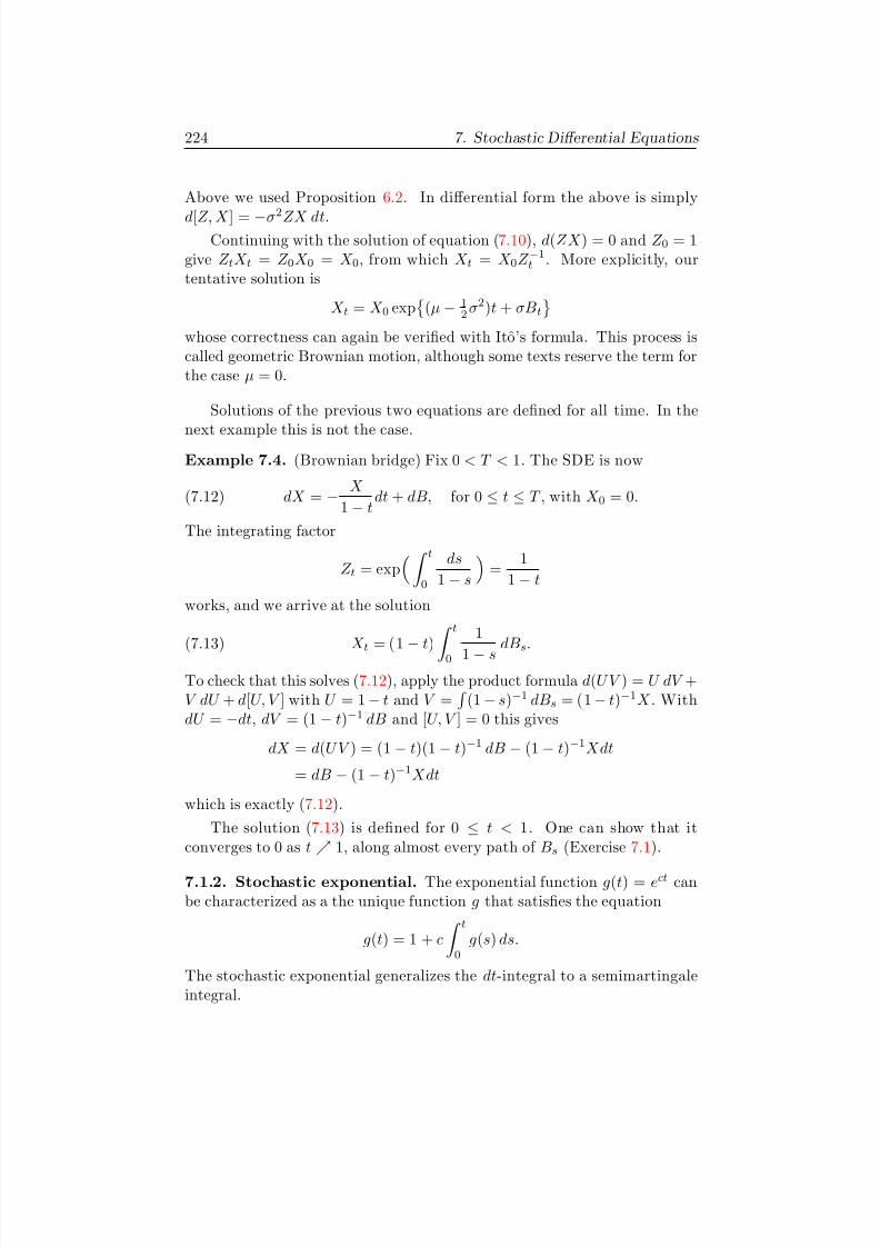
8/3/2019 Basics of Stochastic Analysis
http://slidepdf.com/reader/full/basics-of-stochastic-analysis 228/330
224 7. Stochastic Differential Equations
Above we used Proposition 6.2. In differential form the above is simply
d[Z, X ] = −σ2ZX dt .Continuing with the solution of equation ( 7.10), d(ZX ) = 0 and Z 0 = 1
give Z t X t = Z 0X 0 = X 0, from which X t = X 0Z −1t . More explicitly, our
tentative solution is
X t = X 0 exp (µ − 12 σ2)t + σB t
whose correctness can again be veried with Itˆ o’s formula. This process iscalled geometric Brownian motion, although some texts reserve the term forthe case µ = 0.
Solutions of the previous two equations are dened for all time. In the
next example this is not the case.Example 7.4. (Brownian bridge) Fix 0 < T < 1. The SDE is now
(7.12) dX = −X
1 −tdt + dB, for 0 ≤t ≤T , with X 0 = 0.
The integrating factor
Z t = exp t
0
ds1 −s
=1
1 −t
works, and we arrive at the solution
(7.13) X t = (1
−t)
t
0
1
1 −sdB s .
To check that this solves ( 7.12), apply the product formula d(UV ) = U dV +V dU + d[U, V ] with U = 1 −t and V = (1 −s)−1 dB s = (1 −t)−1X . WithdU = −dt , dV = (1 −t)−1 dB and [U, V ] = 0 this gives
dX = d(UV ) = (1 −t)(1 −t)−1 dB −(1 −t)−1Xdt
= dB −(1 −t)−1Xdt
which is exactly ( 7.12).The solution ( 7.13) is dened for 0 ≤ t < 1. One can show that it
converges to 0 as t 1, along almost every path of B s (Exercise 7.1).
7.1.2. Stochastic exponential. The exponential function g(t) = ect canbe characterized as a the unique function g that satises the equation
g(t) = 1 + c t
0g(s) ds.
The stochastic exponential generalizes the dt-integral to a semimartingaleintegral.

8/3/2019 Basics of Stochastic Analysis
http://slidepdf.com/reader/full/basics-of-stochastic-analysis 229/330
7.1. Examples of stochastic equations and solutions 225
Theorem 7.5. Let Y be a real-valued semimartingale such that Y 0 = 0 .
Dene(7.14) Z t = exp Y t − 1
2 [Y ]ts∈(0 ,t ]
(1 + ∆ Y s )exp −∆ Y s + 12 (∆ Y s )2 .
Then the process Z is a cadlag semimartingale, and it is the unique cadlag semimartingale Z that satises the equation
(7.15) Z t = 1 + (0,t ]Z s−dY s .
Proof. The uniqueness of the solution of ( 7.15) will follow from the generaluniqueness theorem for solutions of semimartingale equations.
We start by showing that Z dened by ( 7.14) is a semimartingale. Thedenition can be reorganized as
Z t = exp Y t − 12 [Y ]t + 1
2s∈(0,t ]
(∆ Y s )2
s∈(0 ,t ]
(1 + ∆ Y s )exp −∆ Y s .
The continuous part
[Y ]ct = [Y ]t −s∈(0,t ]
(∆ Y s )2
of the quadratic variation is an increasing process (cadlag, nondecreasing),hence an FV process. Since ex is a C 2 function, the factor
(7.16) exp( W t ) ≡exp Y t − 12 [Y ]t + 1
2s∈(0,t ]
(∆ Y s )2
is a semimartingale by Itˆ o’s formula. It remains to show that for a xed ωthe product
(7.17) U t ≡s∈(0,t ]
(1 + ∆ Y s )exp −∆ Y s
converges and has paths of bounded variation. The part
s∈(0,t ]:|∆ Y (s)|≥1/ 2
(1 + ∆ Y s )exp −∆ Y s
has only nitely many factors because a cadlag path has only nitely many jumps exceeding a given size in a bounded time interval. Hence this part ispiecewise constant, cadlag and in particular FV. Let ξs = ∆ Y s 1|∆ Y (s)|< 1/ 2denote a jump of magnitude below 1
2 . It remains to show that
H t =s∈(0,t ]
(1 + ξs )exp −ξs = exps∈(0 ,t ]
log(1 + ξs ) −ξs

8/3/2019 Basics of Stochastic Analysis
http://slidepdf.com/reader/full/basics-of-stochastic-analysis 230/330
226 7. Stochastic Differential Equations
is an FV process. For |x| < 1/ 2,
log(1 + x) −x ≤x2.
Hence the sum above is absolutely convergent:
s∈(0 ,t ]
log(1 + ξs ) −ξs ≤s∈(0,t ]
ξ2s ≤[Y ]t < ∞.
It follows that log H t is a cadlag FV process (see Example 1.14 in this con-text). Since the exponential function is locally Lipschitz, H t = exp(log H t )is also a cadlag FV process (Lemma A.6).
To summarize, we have shown that eW t in (7.16) is a semimartingaleand U t in (7.17) is a well-dened real-valued FV process. ConsequentlyZ t = eW t U t is a semimartingale.
The second part of the proof is to show that Z satises equation ( 7.15).Let f (w, u ) = ewu, and nd
f w = f , f u = ew , f uu = 0, f uw = ew and f ww = f .
Note that ∆ W s = ∆ Y s because the jump in [ Y ] at s equals exactly (∆ Y s )2.A straight-forward application of Itˆ o gives
Z t = 1 + (0 ,t ]eW (s−) dU s + (0 ,t ]
Z s−dW s
+ 12 (0,t ]
Z s−d[W ]s + (0,t ]eW (s−) d[W, U ]s
+s∈(0,t ]
∆ Z s −Z s−∆ Y s −eW (s−)∆ U s − 12 Z s−(∆ Y s )2 −eW (s−)∆ Y s ∆ U s .
Since
W t = Y t − 12 [Y ]t −
s∈(0 ,t ]
(∆ Y s )2
where the part in parentheses is FV and continuous, linearity of covariationand Lemma A.10 imply [W ] = [Y ] and [W, U ] = [Y, U ] = ∆ Y ∆ U .
Now match up and cancel terms. First,
(0,t ]eW (s−) dU s −
s∈(0 ,t ]
eW (s−)∆ U s = 0
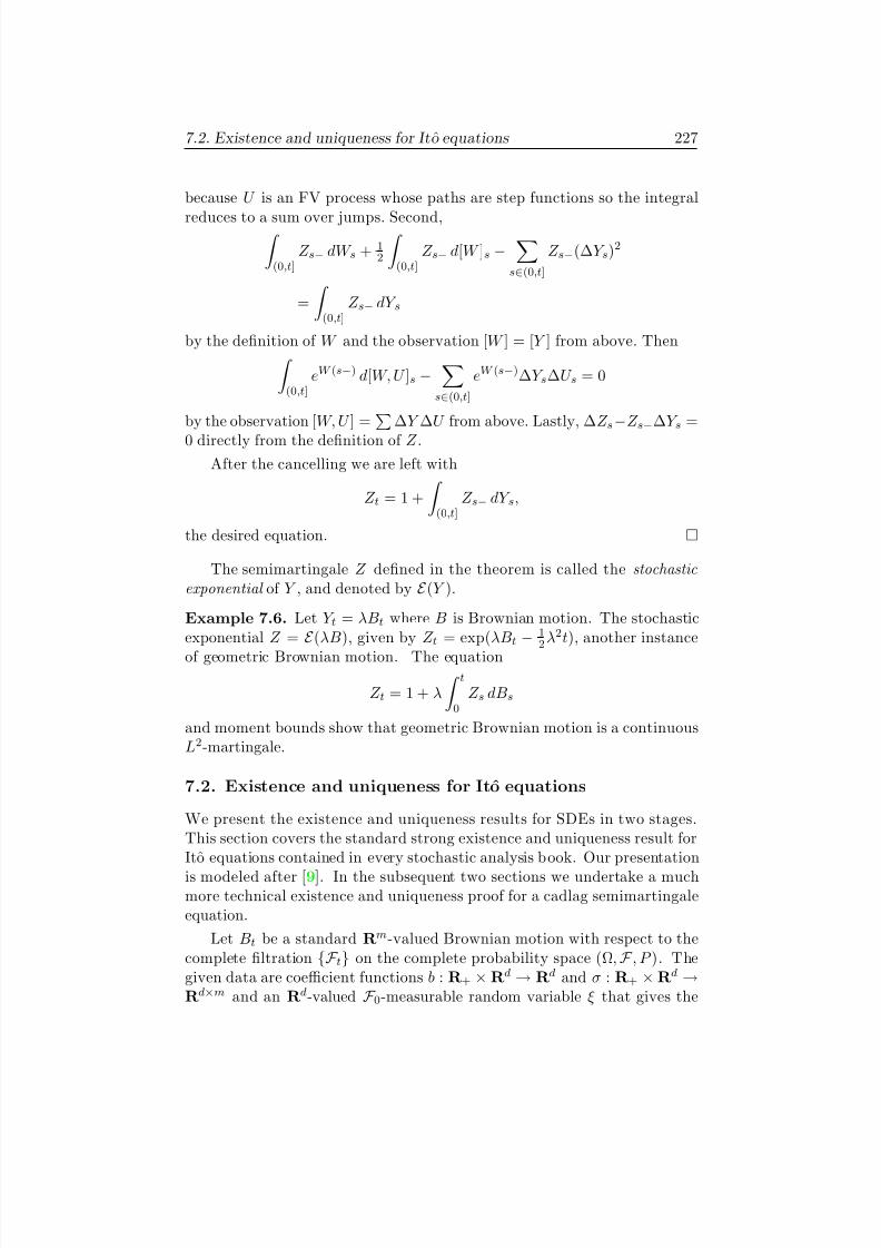
8/3/2019 Basics of Stochastic Analysis
http://slidepdf.com/reader/full/basics-of-stochastic-analysis 231/330
7.2. Existence and uniqueness for Itˆ o equations 227
because U is an FV process whose paths are step functions so the integral
reduces to a sum over jumps. Second,
(0 ,t ]Z s−dW s + 1
2 (0,t ]Z s−d[W ]s −
s∈(0,t ]
Z s−(∆ Y s )2
= (0 ,t ]Z s−dY s
by the denition of W and the observation [ W ] = [Y ] from above. Then
(0 ,t ]eW (s−) d[W, U ]s −
s∈(0,t ]
eW (s−)∆ Y s ∆ U s = 0
by the observation [ W, U ] = ∆ Y ∆ U from above. Lastly, ∆ Z s
−Z s
−∆ Y s =
0 directly from the denition of Z .After the cancelling we are left with
Z t = 1 + (0,t ]Z s−dY s ,
the desired equation.
The semimartingale Z dened in the theorem is called the stochasticexponential of Y , and denoted by E (Y ).
Example 7.6. Let Y t = λB t where B is Brownian motion. The stochasticexponential Z =
E (λB ), given by Z t = exp( λB t
−12 λ2t), another instance
of geometric Brownian motion. The equation
Z t = 1 + λ t
0Z s dB s
and moment bounds show that geometric Brownian motion is a continuousL2-martingale.
7.2. Existence and uniqueness for Itˆ o equations
We present the existence and uniqueness results for SDEs in two stages.This section covers the standard strong existence and uniqueness result forIt o equations contained in every stochastic analysis book. Our presentationis modeled after [ 9 ]. In the subsequent two sections we undertake a muchmore technical existence and uniqueness proof for a cadlag semimartingaleequation.
Let B t be a standard R m -valued Brownian motion with respect to thecomplete ltration F ton the complete probability space (Ω , F , P ). Thegiven data are coefficient functions b : R + ×R d →R d and σ : R + ×R d →R d×m and an R d-valued F 0-measurable random variable ξ that gives the

8/3/2019 Basics of Stochastic Analysis
http://slidepdf.com/reader/full/basics-of-stochastic-analysis 232/330
228 7. Stochastic Differential Equations
initial position. On R d we use the Euclidean norm |x|, and similarly for a
matrix A = ( a i,j ) the norm is |A| = ( |a i,j |2)1/ 2.The goal is to prove that on (Ω , F , P ) there exists an R d-valued process
X that is adapted to F tand satises the integral equation
(7.18) X t = ξ + t
0b(s, X s ) ds + t
0σ(s, X s ) dB s .
in the sense that the processes on the right and left of the equality signare indistinguishable. Part of the requirement is that the integrals are well-dened, for which we require that
(7.19) P ∀T < ∞: T
0 |b(s, X s )|ds + T
0 |σ(s, X s )|2 ds < ∞ = 1 .
Such a process X on (Ω, F , P ) is called a strong solution because it existson the given probability space and is adapted to the given ltration. Stronguniqueness then means that if Y is another process adapted to F tthatsatises ( 7.18)– (7.19), then X and Y are indistinguishable.
Next we state the standard Lipschitz assumption on the coefficient func-tions and then the strong existence and uniqueness theorem.
Assumption 7.7. Assume the Borel functions b : R + ×R d →R d andσ : R + ×R d →R d×m satisfy the Lipschitz condition
(7.20) |b(t, x ) −b(t, y )|+ |σ(t, x ) −σ(t, y )| ≤L|x −y|and the bound
(7.21) |b(t, x )|+ |σ(t, x )| ≤L(1 + |x|)for a constant L < ∞and all t∈R + and x, y∈R d .
Theorem 7.8. Let Assumption 7.7 be in force and let ξ be an R d-valued F 0-measurable random variable. Then there exists a continuous process X on (Ω, F , P ) adapted to F tthat satises integral equation (7.18) and property (7.19). The process X with these properties is unique up to indistinguisha-bility.
Before turning to the proofs we present simple examples from ODEtheory that illustrate the loss of existence and uniqueness when the Lipschitzassumption on the coefficient is weakened.
Example 7.9. (a) Consider the equation
x(t) = t
02 x(s) ds.
The function b(x) = √x is not Lipschitz on [0 , 1] because b (x) blows up atthe origin. The equation has innitely many solutions. Two of them arex(t) = 0 and x(t) = t2.
8/3/2019 Basics of Stochastic Analysis
http://slidepdf.com/reader/full/basics-of-stochastic-analysis 233/330
7.2. Existence and uniqueness for Itˆ o equations 229
(b) The equation
x(t) = 1 + t
0x2(s) ds
does not have a solution for all time. The unique solution starting at t = 0is x(t) = (1 −t)−1 which exists only for 0 ≤ t < 1. The function b(x) = x2 islocally Lipschitz. This is enough for uniqueness, as determined in Exercise7.3.
We prove Theorem 7.8 in stages, and begin with existence under an L2
assumption on the initial state.
Theorem 7.10. Let Assumption 7.7 be in force and the F 0-measurable ini-tial point satisfy
E (|ξ|2) < ∞.Then there exists a continuous process X adapted to F tthat satises in-tegral equation (7.18) and this moment bound: for each T < ∞ there existsa constant C = C (T, L) < ∞such that
(7.22) E (|X t |2) ≤C 1 + E (|ξ|2) for t∈[0, T ].
In particular, the integrand σ(s, X s ) is a member of L2(B ) and
E T
0 |b(s, X s )|2 ds < ∞ for each T < ∞.
Proof of Theorem 7.10 . The existence proof uses classic Picard iteration.We dene a sequence of processes X n indexed by n∈Z + by X 0(t) = ξ andthen for n ≥0
(7.23) X n +1 (t) = ξ + t
0b(s, X n (s)) ds + t
0σ(s, X n (s)) dB s .
Step 1. We show that for each n the process X n is well-dened, con-tinuous, and satises
(7.24) sups∈[0,t ]
E (|X n (s)|2) < ∞ for all t∈R + .
Bound ( 7.24) is clear in the case n = 0 by the denition X 0(t) = ξ andassumption ξ∈L2(P ).
Assume ( 7.24) for n. To show that process X n +1 is well-dened by theintegrals in ( 7.23) we check that, for each t∈R + ,
(7.25) E t
0 |b(s, X n (s))|2 ds + t
0 |σ(s, X n (s)) |2 ds < ∞.
8/3/2019 Basics of Stochastic Analysis
http://slidepdf.com/reader/full/basics-of-stochastic-analysis 234/330
230 7. Stochastic Differential Equations
Assumption ( 7.21) bounds the left side of ( 7.25) by
4L2t 1 + sups∈[0,t ]
E |X n (s)|2which is nite by ( 7.24).
Property ( 7.25) implies that the rst (Lebesgue) integral on the right of (7.23) is a continuous L2 process and that the second (stochastic) integralis a continuous L2 martingale because the integrand lies in L2(B ).
Now we know X n +1 (t) is an L2 random variable. We bound the secondmoment by rst using ( a + b + c)2 ≤ 9(a2 + b2 + c2) and by then apply-ing Schwarz inequality to the rst integral and the isometry of stochasticintegration to the second:
(7.26)
E |X n +1 (t)|2 ≤9E (|ξ|2) + 9 E t
0b(s, X n (s)) ds
2
+ 9 E t
0σ(s, X n (s)) dB s
2
≤9E (|ξ|2) + 9 tE t
0 |b(s, X n (s))|2 ds + 9 E t
0 |σ(s, X n (s))|2 ds
≤9E (|ξ|2) + 18 L2(1 + t)t + 18 L2(1 + t) t
0E |X n (s)|2 ds.
In the last step we applied assumption ( 7.21). Now it is clear that ( 7.24) ispassed from n to n + 1.
Step 2. For each T < ∞there exists a constant A = A(T, L) < ∞suchthat
(7.27) E (|X n (t)|2) ≤A 1 + E (|ξ|2) for all n and t∈[0, T ].
To prove Step 2, restrict t to [0, T ] and introduce a constant C = C (T, L)to rewrite the outcome of ( 7.26) as
E |X n +1 (t)|2 ≤C E (|ξ|2) + 1 + C t
0E |X n (s)|2 ds.
With yn (t) = E |X n (t)|2 we have this situation: there are constants B, C such that
(7.28) y0(t) ≤B and yn +1 (t) ≤B + C t
0yn (s) ds.
This assumption gives inductively
(7.29) yn (t) ≤Bn
k=0
C k tk
k! ≤Be Ct .
This translates into ( 7.27).
8/3/2019 Basics of Stochastic Analysis
http://slidepdf.com/reader/full/basics-of-stochastic-analysis 235/330
7.2. Existence and uniqueness for Itˆ o equations 231
Step 3. There exists a continuous, adapted process X such that X n →X uniformly on compact time intervals both almost surely and in this L2sense: for each T < ∞(7.30) lim
n→∞E sup
0≤s≤T |X (s) −X n (s)|2 = 0 .
Furthermore, X satises moment bound ( 7.22).
For process X n +1 −X n (7.23) gives the equation
(7.31)
X n +1 (t) −X n (t) = t
0b(s, X n (s)) −b(s, X n−1(s)) ds
+
t
0σ(s, X n (s))
−σ(s, X n
−1(s)) dB s
≡Gn (t) + M n (t)
where Gn is an FV process and M n an L2 martingale. Schwarz inequalityand the Lipschitz assumption ( 7.20) give
(7.32)E sup
0≤s≤t|Gn (s)|2 ≤ t t
0E b(s, X n (s)) −b(s, X n−1(s)) 2 ds
≤L2t t
0E |X n (s)) −X n−1(s)|2 ds.
The isometry of stochastic integration and Doob’s inequality (Theorem 3.11)
give
(7.33)
E sup0≤s≤t|M n (s)|2 ≤4E [ |M n (t)|2 ]
= 4 t
0E σ(s, X n (s)) −σ(s, X n−1(s)) 2 ds
≤4L2 t
0E |X n (s)) −X n−1(s)|2 ds.
Restrict t to [0, T ] and combine the above bounds into
(7.34)
E sup0≤s≤t|X n +1 (s) −X n (s)|2
≤C t
0E sup
0≤u≤s|X n (u)) −X n−1(u)|2 ds.
For yn (t) = E sup0≤s≤t |X n +1 (s) −X n (s)|2 we have constants B, C suchthat these inequalities hold for t∈[0, T ]:
(7.35) y0(t) ≤B and yn +1 (t) ≤C t
0yn (s) ds.

8/3/2019 Basics of Stochastic Analysis
http://slidepdf.com/reader/full/basics-of-stochastic-analysis 236/330
232 7. Stochastic Differential Equations
The inequality for y0(t) is checked separately:
y0(t) = E sup0≤s≤t|X 1(s) −X 0(s)|2
= E sup0≤s≤t s
0b(u, ξ ) du + s
0σ(u, ξ ) dBu
2
and reason as above once again.Bounds ( 7.35) develop inductively into
(7.36) yn (t) ≤BC n tn
n!.
An application of Chebyshev’s inequality gives us a summable bound that
we can feed into the Borel-Cantelli lemma:P sup
0≤s≤t|X n +1 (s) −X n (s)| ≥2−n ≤4n E sup0≤s≤t|X n +1 (s) −X n (s)|2
≤B4n C n tn
n!.
Consider now T ∈N . From
nP sup
0≤s≤T |X n +1 (s) −X n (s)| ≥2−n < ∞and the Borel-Cantelli lemma we conclude that for almost every ω and eachT
∈
N there exists a nite N T (ω) <
∞such that n
≥N T (ω) implies
sup0≤s≤T |X n +1 (s) −X n (s)| < 2−n .
Thus for almost every ω the paths X nform a Cauchy sequence in the spaceC [0, T ] of continuous functions with supremum distance, for each T ∈N .This space is complete (Lemma A.5). Consequently there exists a continuouspath X s (ω) : s∈R + , dened for almost every ω, such that
sup0≤s≤T |X (s) −X n (s)| →0 as n → ∞
for all T ∈N and almost every ω. This denes X and proves the almost sureconvergence part of Step 3. Adaptedness of X comes from X n (t)
→X (t)
a.s. and the completeness of the σ-algebra F t .From the uniform convergence we get
sup0≤s≤T |X (s) −X n (s)| = lim
m→∞sup
0≤s≤T |X m (s) −X n (s)|.Abbreviate ηn = sup 0≤s≤T |X n +1 (s) −X n (s)| and let ηn 2 = E (η2
n )1/ 2 de-note L2 norm. By Fatou’s lemma and the triangle inequality for the L2
8/3/2019 Basics of Stochastic Analysis
http://slidepdf.com/reader/full/basics-of-stochastic-analysis 237/330
7.2. Existence and uniqueness for Itˆ o equations 233
norm,
sup0≤s≤T |X (s) −X n (s)| 2 ≤ lim
m→∞sup
0≤s≤T |X m (s) −X n (s)| 2
≤ limm→∞
m−1
k= n
ηk 2 =∞
k= n
ηk 2.
By estimate ( 7.36) the last expression vanishes as n → ∞. This gives ( 7.30).Finally, L2 convergence (or Fatou’s lemma) converts ( 7.27) into ( 7.22). Thiscompletes the proof of Step 3.
Step 4. Process X satises ( 7.18).
The integrals in ( 7.18) are well-dened continuous processes because
we have established the L2 bound on X that gives the L2 bounds on theintegrands as in the last step of ( 7.26). To prove Step 4 we show that theterms in ( 7.23) converge to those of ( 7.18) in L2. We have derived therequired estimates already. For example, by the Lipschitz assumption and(7.30), for every T < ∞,
E T
0σ(s, X n (s)) −σ(s, X (s)) 2 ds ≤L2E T
0 |X n (s) −X (s)|2 ds →0.
This says that the integrand σ(s, X n (s)) converges to σ(s, X (s)) in the space
L2(B ). Consequently we have the L2 convergence of stochastic integrals:
t
0
σ(s, X n (s)) dB s
→ t
0
σ(s, X (s)) dB s
which also holds uniformly on compact time intervals.We leave the argument for the other integral as an exercise. Proof of
Theorem 7.10 is complete.
At this point we prove strong uniqueness. We prove a slightly moregeneral result which we can use also to extend the existence result beyondξ∈L2(P ). Let η be another initial condition and Y a process that satises
(7.37) Y t = η + t
0b(s, Y s ) ds + t
0σ(s, Y s ) dB s .
Theorem 7.11. Let ξ and η be R d-valued
F 0-measurable random variables
without any integrability assumptions. Assume that coefficients b and σ areBorel functions that satisfy Lipschitz condition (7.20). Let X and Y betwo continuous processes on (Ω, F , P ) adapted to F t. Assume X satisesintegral equation (7.18) and condition (7.19). Assume Y satises integral equation (7.37) and condition (7.19) with X replaced by Y . Then on theevent ξ = ηprocesses X and Y are indistinguishable. That is, for almost every ω such that ξ(ω) = η(ω), X t (ω) = Y t (ω) for all t∈R + .
8/3/2019 Basics of Stochastic Analysis
http://slidepdf.com/reader/full/basics-of-stochastic-analysis 238/330
234 7. Stochastic Differential Equations
In the case η = ξ we get the strong uniqueness. The uniqueness state-
ment is actually true with a weaker local Lipschitz condition (Exercise 7.3).Corollary 7.12. Let ξ be an R d-valued F 0-measurable random variable.Assume that b and σ are Borel functions that satisfy Lipschitz condition (7.20). Then up to indistinguishability there is at most one continuous pro-cess X on (Ω, F , P ) adapted to F tthat satises (7.18)– (7.19).
For the proof of Theorem 7.11 we introduce a basic tool from analysis.
Lemma 7.13. (Gronwall’s inequality) Let g be an integrable Borel function on [a, b], f a nondecreasing function on [a, b], and assume that there existsa constant B such that
g(t) ≤f (t) + B t
ag(s) ds, a ≤ t ≤b.
Then g(t) ≤f (t)eB (t−a) , a ≤t ≤b.
Proof. The integral ta g(s) ds of an integrable function g is an absolutely
continuous (AC) function of the upper limit t. At Lebesgue-almost every tit is differentiable and the derivative equals g(t). Consequently the equation
ddt e−
Bt
t
a g(s) ds = −Be −Bt
t
a g(s) ds + e−Bt
g(t)is valid for Lebesgue-almost every t. Hence by the hypothesis
ddt
e−Bt t
ag(s) ds = e−Bt g(t) −B t
ag(s) ds
≤f (t)e−Bt for almost every t.
An absolutely continuous function is the integral of its almost everywhereexisting derivative. Integrating above and using the monotonicity of f give
e−Bt
t
ag(s) ds ≤
t
af (s)e−Bs ds ≤
f (t)B
e−Ba −e−Bt
from which
t
ag(s) ds ≤
f (t)B
eB (t−a) −1 .
Using the assumption once more,
g(t) ≤f (t) + B ·f (t)B
eB (t−a) −1 = f (t)eB (t−a) .

8/3/2019 Basics of Stochastic Analysis
http://slidepdf.com/reader/full/basics-of-stochastic-analysis 239/330
7.2. Existence and uniqueness for Itˆ o equations 235
Proof of Theorem 7.11 . In order to use L2 bounds we stop the processes
before they get too large. Fix n∈
N for the time being and dene
ν = inf t ≥0 : |X t −ξ| ≥n or |Y t −η| ≥n.
This is a stopping time by Corollary 2.10. Processes X τ −ξ and Y τ −η arebounded.
The bounded F 0-measurable random variable 1η = ξmoves freely inand out of a stochastic integrals. This can be seen for example from theconstructions themselves. By subtracting the equations for X t and Y t andthen stopping we get this equation:
(7.38)
(X ν
t −Y ν
t ) ·1
η = ξ= ν ∧t
0b(s, X s ) −b(s, Y s ) 1η = ξds
+ ν ∧t
0σ(s, X s ) −σ(s, Y s ) 1η = ξdB s
= ν ∧t
0b(s, X ν
s ) −b(s, Y ν s ) 1η = ξds
+ ν ∧t
0σ(s, X ν
s ) −σ(s, Y ν s ) 1η = ξdB s
≡G(t) + M (t).
The last equality denes the processes G and M . The next to last equalitycomes from the fact that if integrands agree up to a stopping time, then sodo stochastic integrals (Proposition 4.10(c) for Brownian motion). We havethe constant bound
σ(s, X ν s ) −σ(s, Y ν
s ) ·1η = ξ ≤L|X ν s −Y ν
s | ·1η = ξ≤ L|(X ν
s −ξ) −(Y ν s −η)| ·1η = ξ ≤2Ln
and similarly for the other integrand. Consequently G is an L2 FV processand M an L2 martingale.
Schwarz inequality, bounding ν ∧
t above with t, and the Lipschitz as-sumption ( 7.20) give
E |G(t)|2 ≤ t t
0E |b(s, X ν
s ) −b(s, Y ν s )|2 1η = ξ ds
≤L2t t
0E |X ν
s −Y ν s |2 1η = ξ ds.

8/3/2019 Basics of Stochastic Analysis
http://slidepdf.com/reader/full/basics-of-stochastic-analysis 240/330
236 7. Stochastic Differential Equations
The isometry of stochastic integration gives
E |M (t)|2 = E ν ∧t
0σ(s, X ν
s ) −σ(s, Y ν s ) 1η = ξdB s
2
= E t
01 [0,ν ](t) σ(s, X ν
s ) −σ(s, Y ν s ) 1η = ξdB s
2
= t
0E 1 [0,ν ](t)|σ(s, X ν
s ) −σ(s, Y ν s )|2 1η = ξ ds
≤L2 t
0E |X ν
s −Y ν s |2 1η = ξ ds.
In the second equality above we moved the cut-off at ν from the upper limitinto the integrand in accordance with ( 5.23) from Proposition 5.16. (Strictlyspeaking we have proved this only for predictable integrands but naturallythe same property can be proved for the more general Brownian motionintegral.)
Combine the above bounds into
E |X ν t −Y ν
t |2 1η = ξ ≤2L2(t + 1) t
0E |X ν
s −Y ν s |2 1η = ξ ds.
If we restrict t to [0, T ] we can replace 2L2(t + 1) with the constant B =2L2(T + 1) above. Then Gronwall’s inequality implies
E |X ν t −Y ν
t |2 1η = ξ = 0 for t∈[0, T ].
We can repeat this argument for each T ∈
N and so extend the conclusion toall t∈R . Thus on the event η = ξ the continuous processes X ν and Y ν agreealmost surely at each xed time. It follows that they are indistinguishable.Now we have this statement for each n that appears in the denition of ν .With continuous paths we have ν ∞as we take n to innity. In the endwe can conclude that X and Y are indistinguishable on the event η = ξ.
Completion of the proof of Theorem 7.8 . It remains to remove the as-sumption ξ∈L2(P ) from the existence proof. Let X m (t) be the solutiongiven by Theorem 7.10 for the initial point ξ1|ξ| ≤ m. By Theorem7.11, for m < n processes X m and X n are indistinguishable on the event
|ξ
| ≤m
. Thus we can consistently dene
X (t) = X m (t) on the event |ξ| ≤m.
X has continuous paths because each X m does, and adaptedness of X canbe checked because |ξ| ≤m ∈ F 0. X satises ( 7.19) because each X mdoes. Thus the integrals in ( 7.18) are well-dened for X .
To verify equation ( 7.18) we can again pass the F 0-measurable indicator1|ξ| ≤m in and out of stochastic integrals, and then use the equality
8/3/2019 Basics of Stochastic Analysis
http://slidepdf.com/reader/full/basics-of-stochastic-analysis 241/330
7.2. Existence and uniqueness for Itˆ o equations 237
of processes b(s, X (s))1|ξ| ≤m= b(s, X m (s))1|ξ| ≤mwith the same
property for σ:X (t)1|ξ| ≤m= X m (t)1|ξ| ≤m= ξ1|ξ| ≤m+ t
0b(s, X m (s))1|ξ| ≤mds
+ t
0σ(s, X m (s))1|ξ| ≤mdB s
= ξ1|ξ| ≤m+ t
0b(s, X (s))1|ξ| ≤mds
+
t
0σ(s, X (s))1|ξ| ≤mdB s
= 1|ξ| ≤m ξ + t
0b(s, X (s)) ds +
t
0σ(s, X (s)) dB s .
Since the union of the events |ξ| ≤mis the entire space (almost surely),we have the equation for X .

8/3/2019 Basics of Stochastic Analysis
http://slidepdf.com/reader/full/basics-of-stochastic-analysis 242/330
238 7. Stochastic Differential Equations
7.3. A semimartingale equation
Fix a probability space (Ω , F , P ) with a ltration F t. We consider theequation
(7.39) X (t, ω) = H (t, ω) + (0,t ]F (s ,ω,X (ω)) dY (s, ω)
where Y is a given R m -valued cadlag semimartingale, H is a given R d-valued adapted cadlag process, and X is the unknown R d-valued process.The coefficient F is a d ×m-matrix valued function of its arguments. (Thecomponentwise interpretation of the stochastic integral F dY appearedRemark 5.38.) For the coefficient F we make these assumptions.
Assumption 7.14. The coefficient function F (s ,ω,η) in equation ( 7.39) isa measurable function from the space R + ×Ω ×DR d [0, ∞) into the spaceR d×m of d ×m matrices, and satises the following requirements.
(i) F satises a spatial Lipschitz condition uniformly in the other vari-ables: there exists a nite constant L such that this holds for all(t, ω)∈R + ×Ω and all η, ζ ∈DR d [0, ∞):
(7.40) |F (t ,ω,η) −F (t ,ω,ζ )| ≤L · sups∈[0,t )|η(s) −ζ (s)|.
(ii) Given any adapted R d-valued cadlag process X on Ω, the function(t, ω) →F (t ,ω,X (ω)) is a predictable process.
(iii) Given any adapted R d-valued cadlag process X on Ω, there existstopping times ν k ∞such that 1 (0 ,ν k ](t)F (t, X ) is bounded foreach k.
These conditions on F are rather technical. They are written to helpprove the next theorem. The proof is lengthy and postponed to the nextsection. There are technical steps where we need right-continuity of theltration, hence we include this requirement in the hypotheses.
Theorem 7.15. Assume F t is complete and right-continuous. Let H be an adapted R d-valued cadlag process and Y an R m -valued cadlag semi-martingale. Assume F satises Assumption 7.14. Then there exists a cadlag process X (t) : 0 ≤ t < ∞adapted to F tthat satises equation (7.39),and X is unique up to indistinguishability.
In the remainder of this section we discuss the assumptions on F andstate some consequences of the existence and uniqueness theorem.
Notice the exclusion of the endpoint t on the right-hand side of theLipschitz condition ( 7.40). This implies that F (t,ω, ·) is a function of the
8/3/2019 Basics of Stochastic Analysis
http://slidepdf.com/reader/full/basics-of-stochastic-analysis 243/330
7.3. A semimartingale equation 239
stopped path
ηt−(s) =η(0) , t = 0 , 0 ≤s < ∞η(s), 0 ≤s < t
η(t−), s ≥ t > 0.In other words, the function F (t,ω, ·) only depends on the path on the timeinterval [0 , t ).
Parts (ii)–(iii) guarantees that the stochastic integral F (s, X ) dY (s)exists for an arbitrary adapted cadlag process X and semimartingale Y .The existence of the stopping times ν kin part (iii) can be veried via thislocal boundedness condition.
Lemma 7.16. Assume F satises parts (i) and (ii) of Assumpotion 7.14.
Suppose there exists a path ζ ∈
D R d [0, ∞) such that for all T < ∞,(7.41) c(T ) = sup
t∈[0,T ], ω∈Ω|F (t,ω, ζ )| < ∞.
Then for any adapted R d-valued cadlag process X there exist stopping timesν k ∞such that 1 (0 ,ν k ](t)F (t, X ) is bounded for each k.
Proof. Dene
ν k = inf t ≥0 : |X (t)| ≥k∧inf t > 0 : |X (t−)| ≥k∧kThese are bounded stopping times by Lemma 2.9. |X (s)| ≤k for 0 ≤s < ν k ,but if ν k = 0 we cannot claim that |X (0) | ≤k. The stopped process
X ν k −(t) =X (0) , ν k = 0X (t), 0 ≤ t < ν kX (ν k−), t ≥ν k > 0
is cadlag and adapted.We show that 1 (0 ,ν k ](s)F (s, X ) is bounded. If s = 0 or ν k = 0 then this
random variable vanishes. Suppose 0 < s ≤ ν k . Since [0, s) ⊆[0, ν k), X agrees with X ν k − on [0, s), and then F (s, X ) = F (s, X ν k −) by (7.40).
|F (s, X )| = |F (s, X ν k −)| ≤ |F (s, ζ )|+ |F (s, X ν k −) −F (s, ζ )|≤c(k) + L · sup
0≤t<ν k |X (t) −ζ (t)|≤c(k) + L k + sup
0≤t≤k|ζ (t)| .
The last line above is a nite quantity because ζ is locally bounded, beinga cadlag path.
Here is how to apply the theorem to an equation that is not dened forall time.

8/3/2019 Basics of Stochastic Analysis
http://slidepdf.com/reader/full/basics-of-stochastic-analysis 244/330
240 7. Stochastic Differential Equations
Corollary 7.17. Let 0 < T < ∞. Assume F t is right-continuous, Y
is a cadlag semimartingale and H is an adapted cadlag process, all dened for 0 ≤ t ≤ T . Let F satisfy Assumption 7.14 for (t, ω) ∈[0, T ] ×Ω. In particular, part (ii) takes this form: if X is a predictable process dened on [0, T ] ×Ω, then so is F (t, X ), and there is a nondecreasing sequence of stopping times σksuch that 1 (0 ,σk ](t)F (t, X ) is bounded for each k, and for almost every ω, σk = T for all large enough k.
Then there exists a unique solution X to equation (7.39) on [0, T ].
Proof. Extend the ltration, H , Y and F to all time in this manner: fort∈(T,∞) and ω∈Ω dene F t = F T , H t (ω) = H T (ω), Y t (ω) = Y T (ω), andF (t ,ω,η) = 0. Then the extended processes H and Y and the coefficient F
satisfy all the original assumptions on all of [0 , ∞). Note in particular thatif G(t) = F (t, X ) is a predictable process for 0 ≤ t ≤ T , then extendingit as a constant to ( T,∞) produces a predictable process for 0 ≤ t < ∞.And given a predictable process X on [0, ∞), let σkbe the stopping timesgiven by the assumption, and then dene
ν k =σk , σk < T
∞, σk = T.
These stopping times satisfy part (iii) of Assumption 7.14 for [0, ∞). NowTheorem 7.39 gives a solution X for all time 0 ≤ t < ∞ for the extendedequation, and on [0 , T ] X solves the equation with the original H , Y and F .
For the uniqueness part, given a solution X of the equation on [0 , T ],extend it to all time by dening X t = X T for t ∈(T,∞). Then we havea solution of the extended equation on [0 , ∞), and the uniqueness theoremapplies to that.
Another easy generalization is to the situation where the Lipschitz con-stant is an unbounded function of time.
Corollary 7.18. Let the assumptions be as in Theorem 7.15 , except that the Lipschitz assumption is weakened to this: for each 0 < T < ∞ thereexists a nite constant L(T ) such that this holds for all (t, ω)∈[0, T ] ×Ωand all η, ζ
∈
DR
d [0,
∞):
(7.42) |F (t ,ω,η) −F (t ,ω,ζ )| ≤L(T ) · sups∈[0,t )|η(s) −ζ (s)|.
Then equation (7.39) has a unique solution X adapted to F t.
Proof. For k∈N , the function 10≤t≤kF (t ,ω,η) satises the original hy-potheses. By Theorem 7.15 there exists a process X k that satises the

8/3/2019 Basics of Stochastic Analysis
http://slidepdf.com/reader/full/basics-of-stochastic-analysis 245/330
7.3. A semimartingale equation 241
equation
(7.43) X k (t) = H k (t) + (0 ,t ]1 [0,k ](s)F (s, X k) dY k (s).
The notation above is H k (t) = H (k∧t) for a stopped process as before. Letk < m . Stopping the equation
X m (t) = H m (t) + (0 ,t ]1 [0,m ](s)F (s, X m ) dY m (s)
at time k gives the equation
X km (t) = H k (t) + (0 ,t∧k]1 [0,m ](s)F (s, X m ) dY m (s),
valid for all t. By Proposition 5.39 stopping a stochastic integral can beachieved by stopping the integrator or by cutting off the integrand with anindicator function. If we do both, we get the equation
X km (t) = H k (t) + (0 ,t ]1 [0,k ](s)F (s, X km ) dY k (s).
Thus X k and X km satisfy the same equation, so by the uniqueness theorem,X k = X km for k < m . Thus we can unambiguously dene a process X bysetting X = X k on [0, k]. Then for 0 ≤ t ≤k we can substitute X for X k inequation ( 7.43) and get the equation
X (t) = H k (t) +
(0 ,k
∧
t ]F (s, X ) dY (s), 0 ≤ t ≤k.
Since this holds for all k, X is a solution to the original SDE ( 7.39).Uniqueness works similarly. If X and X solve (7.39), then X (k∧t) and
X (k∧t) solve (7.43). By the uniqueness theorem X (k∧t ) = X (k∧t) forall t, and since k can be taken arbitrary, X = X .
Example 7.19. Here are ways by which a coefficient F satisfying the as-sumptions of Corollary 7.18 can arise.
(i) Let f (t ,ω,x ) be a P⊗BR d -measurable function from ( R + ×Ω)×R d
into d ×m-matrices. Assume f satises the Lipschitz condition
|f (t ,ω,x ) −f (t ,ω,y)| ≤L(T )|x −y|for (t, ω)
∈[0, T ]×Ω and x, y
∈R d , and the local boundedness condition
sup |f (t,ω, 0)| : 0 ≤t ≤T, ω∈Ω < ∞for all 0 < T < ∞. Then put F (t ,ω,η) = f (t ,ω,η(t−)).
Satisfaction of the conditions of Assumption 7.14 is straight-forward,except perhaps the predictability. Fix a cadlag process X and let U bethe space of P ⊗ BR d -measurable f such that ( t, ω) →f (t ,ω,X t−(ω)) is

8/3/2019 Basics of Stochastic Analysis
http://slidepdf.com/reader/full/basics-of-stochastic-analysis 246/330
242 7. Stochastic Differential Equations
P -measurable. This space is linear and closed under pointwise convergence.
By Theorem B.2 it remains to check that U contains indicator functionsf = 1 Γ×B of products of Γ ∈ P and B∈ BR d . For such f , f (t ,ω,X t−(ω)) =1 Γ (t, ω)1 B (X t−(ω)). The rst factor 1 Γ(t, ω) is predictable by construction.The second factor 1 B (X t−(ω)) is predictable because X t− is a predictableprocess, and because of the general fact that g(Z t ) is predictable for anypredictable process Z and any measurable function g on the state space of Z .
(ii) A special case of the preceding is a Borel measurable function f (t, x )on [0, ∞) ×R d with the required Lipschitz and boundedness conditions. Inother words, no dependence on ω.
(iii) Continuing with non-random functions, suppose a function G :D R d [0, ∞) →DR d [0, ∞) satises a Lipschitz condition in this form:
(7.44) G(η) t −G(ζ )t ≤L · sups∈[0,t )|η(s) −ζ (s)|.
Then F (t ,ω,η) = G(η)t− satises Assumption 7.14.
Next, let us specialize to Itˆo equations to recover Theorem 7.8 proved inSection 7.2.
Corollary 7.20. Let B t be a standard Brownian motion in R m with respect to a right-continuous ltration F tand ξ an R d-valued F 0-measurable ran-dom variable. Fix 0 < T <
∞. Assume the functions b : [0, T ]
×R d
→R d
and σ : [0, T ] ×R d →R d×m satisfy the Lipschitz condition
|b(t, x ) −b(t, y )|+ |σ(t, x ) −σ(t, y )| ≤L|x −y|and the bound
|b(t, x )|+ |σ(t, x )| ≤L(1 + |x|) for a constant L and all 0 ≤ t ≤T , x, y∈R d .
Then there exists a unique continuous process X on [0, T ] that is adapted to F tand satises
(7.45) X t = ξ + t
0b(s, X s ) ds + t
0σ(s, X s ) dB s
for 0 ≤ t ≤T .Proof. To t this into Theorem 7.15, let Y (t) = [ t, B t ]T , H (t) = ξ, and
F (t ,ω,η) = b(t, η(t−)) , σ(t, η(t−)) .
We write b(t, η(t−)) to get a predictable coefficient. For a continuous pathη this left limit is immaterial as η(t−) = η(t). The hypotheses on b and σestablish the conditions required by the existence and uniqueness theorem.
8/3/2019 Basics of Stochastic Analysis
http://slidepdf.com/reader/full/basics-of-stochastic-analysis 247/330
7.4. Existence and uniqueness for a semimartingale equation 243
Once there is a cadlag solution X from the theorem, continuity of X follows
by observing that the right-hand side of ( 7.45) is a continuous process.
7.4. Existence and uniqueness for a semimartingale equation
This section proves Theorem 7.15. The key part of both the existence anduniqueness proof is a Gronwall-type estimate, which we derive after sometechnical preliminaries. Note that we can assume the Lipschitz constantL > 0. If L = 0 then F (s ,ω,X ) does not depend on X , equation ( 7.39)directly denes the process X and there is nothing to prove.
7.4.1. Technical preliminaries.
Lemma 7.21. Let X be a cadlag process and Y a cadlag semimartingale.Fix t > 0. Let γ be a nondecreasing continuous process on [0, t ] such that γ (0) = 0 and γ (u) is a stopping time for each u. Then
(7.46) (0 ,γ (t )]X (s−) dY (s) = (0 ,t ]
X γ (s−) d(Y γ )(s).
Remark 7.22. On the right the integrand is
X γ (s−) = limu s,u<s
X (γ (u))
which is not the same as X (γ (s−)) if the latter is interpreted as X evaluatedat γ (s
−). To see this just think of γ (u) = u and imagine X has a jump at
s. Note that for the stochastic integral on the right in ( 7.46) the ltrationchanged to F γ (u ).
Proof. As tni goes through partitions of [0 , t ] with mesh tending to zero,
γ (tni )goes through partitions of [0 , γ (t)] with mesh tending to zero. By
Proposition 5.37, both sides of (7.46) equal the limit of the sums
i
X (γ (tni )) Y (tn
i+1 ) −Y (tni ) .
Lemma 7.23. Suppose A is a nondecreasing cadlag function such that A(0) = 0 , and Z is a nondecreasing real-valued cadlag function. Then
γ (u) = inf
t
≥0 : A(t) > u
denes a nondecreasing cadlag function with γ (0) = 0 , and
(0,u ]Z γ (s−) d(A γ )( s) ≤ A(γ (u)) −u Z γ (u−)
+ (0,u ]Z γ (s−) ds.
(7.47)
8/3/2019 Basics of Stochastic Analysis
http://slidepdf.com/reader/full/basics-of-stochastic-analysis 248/330
244 7. Stochastic Differential Equations
Proof. That γ is nondecreasing is immediate. To see right-continuity, let
s > γ (u). Then A(s) > u . Pick ε > 0 so that A(s) > u + ε. Then forv∈[u, u + ε], γ (v) ≤s.
Also, since A(t) > u for t > γ (u), by the cadlag property of A
(7.48) A(γ (u)) ≥u.
Since Z γ is cadlag, the integrals ( 7.47) are limits of Riemann sums withintegrand evaluated at the left endpoint of partition intervals (Lemma 1.12).Let 0 = s0 < s 1 < · · ·< s m = ube a partition of [0 , u]. Next algebraicmanipulations:
m−1
i=0
Z (γ (s i )) A(γ (s i+1 )) −A(γ (s i ))
=m−1
i=0
Z (γ (s i ))( s i+1 −s i )
+m−1
i=0
Z (γ (s i )) A(γ (s i+1 )) −s i+1 −A(γ (s i)) + s i
=m−1
i=0
Z (γ (s i ))( s i+1 −s i ) + Z (γ (sm−1)) A(γ (u)) −u
−m−1
i=1
Z (γ (s i)) −Z (γ (s i−1)) A(γ (s i )) −s i .
The sum on the last line above is nonnegative by the nondecreasing mono-tonicity of Z γ and by ( 7.48). Thus we have
m−1
i=0Z (γ (s i )) A(γ (s i+1 )) −A(γ (s i ))
≤m−1
i=0Z (γ (s i ))( s i+1 −s i ) + Z (γ (sm−1)) A(γ (u)) −u .
Letting the mesh of the partition to zero turns the inequality above into(7.47).
Let F be a cadlag BV function on [0 , T ] and ΛF its Lebesgue-Stieltjesmeasure. The total variation function of F was denoted by V F (t). The totalvariation measure |ΛF | satises |ΛF | = Λ V F . For Lebesgue-Stieltjes integralsthe general inequality ( 1.11) for signed measures can be written in this form:
(7.49) (0 ,T ]g(s) dF (s) ≤ (0,T ]|g(s)|dV F (s).

8/3/2019 Basics of Stochastic Analysis
http://slidepdf.com/reader/full/basics-of-stochastic-analysis 249/330
7.4. Existence and uniqueness for a semimartingale equation 245
Lemma 7.24. Let X be an adapted cadlag process and α > 0. Let τ 1 <
τ 2 < τ 3 < · · ·be the times of successive jumps in X of magnitude above α:with τ 0 = 0 ,
τ k = inf t > τ k−1 : |X (t) −X (t−)| > α .Then the τ kare stopping times.
Proof. Fix k. We show τ k ≤ t ∈ F t . Consider the event
A =
≥1 m ≥1 N ≥1 n≥N
there exist integers 0 < u 1 < u 2 < · · ·< u k ≤n
such that u i −u i−1 ≥n/ , and
X u i t
n −X
u i t
n −t
n> α +
1
m.
We claim that A = τ k ≤ t.Suppose ω ∈A. Let sn,i = u i t/n , 1 ≤ i ≤ k, be the points whose
existence follows for all n ≥ N . Pass to a subsequence n j such that foreach 1 ≤ i ≤ k we have convergence sn j ,i →t i ∈[0, t ] as j → ∞. Fromthe description of A there is an 1 ≤ < ∞ such that t i −t i−1 ≥ t/ . Theconvergence also forces sn j ,i −t/n →t i . Since the increment in the path X cannot shrink below α + 1 /m across the two points sn j ,i −t/n and sn j ,i , itmust be the case that |X (t i ) −X (t i−)| ≥α + 1 /m .
Consequently the points t1, t2, . . . , t k are times of jumps of magnitudeabove α, and thereby τ k
≤t .
Conversely, suppose ω∈ τ k ≤ tand let t1 < t 2 < · · ·< t k be times of
jumps of magnitude above α in [0, t ]. Pick ε > 0 so that |X (t i ) −X (t i−)| ≥α +2 ε and t i −t i−1 > 4ε for 2 ≤ i ≤k. Pick δ∈(0, ε) such that r∈[t i −δ, t i )and s∈[t i , t i + δ] imply
|X (s) −X (r )| > α + ε.
Now let > t/ε , m > 1/ε and N > t/δ . Then for n ≥ N nd integers u isuch that
(u i −1)tn
< t i ≤u itn
.
Then alsoti −
δ < (ui −
1)t
n< t
i ≤u
i
t
n< t
i+ δ
from whichX
u i tn −X
u i tn −
tn
> α +1m
.
This shows ω∈A.
We need to consider equations for stopped processes, and also equationsthat are “restarted” at a stopping time.

8/3/2019 Basics of Stochastic Analysis
http://slidepdf.com/reader/full/basics-of-stochastic-analysis 250/330
246 7. Stochastic Differential Equations
Lemma 7.25. Suppose F satises Assumption 7.14 and let
ξ(t) = (0,t ]F (s, X ) dY (s).
Let τ be a nite stopping time. Then
(7.50) ξτ −(t) = (0 ,t ]F (s, X τ −) dY τ −(s).
In particular, suppose X satises equation (7.39). Then the equation con-tinues to hold when all processes are stopped at τ −. In other words,
(7.51) X τ −(t) = H τ −(t) + (0 ,t ]F (s, X τ −) dY τ −(s).
Proof. It suffices to check (7.50), the second conclusion is then immediate.Apply part (b) of Proposition 5.50 with G(s) = F (s, X τ −) and J (s) =F (s, X ). By the precise form of the Lipschitz property ( 7.40) of F , which istrue for each xed ω, for 0 ≤s ≤τ we have
|F (s, X τ −) −F (s, X )| ≤L · supu∈[0,s )|X τ −s −X s |
≤L · supu∈[0,τ )|X s −X s | = 0 .
Then rst by part (b), then by part (a) of Proposition 5.50,
ξτ
− = ( J ·Y )τ
− = ( G ·Y )τ
− = G ·Y τ
−.Lemma 7.26. Assume the ltration F tis right-continuous. Let σ be a nite stopping time for F tand ¯F t = F σ+ t .
(a) Let ν be a stopping time for ¯F t. Then σ + ν is a stopping time for
F tand ¯F ν ⊆ F σ+ ν .(b) Suppose τ is a stopping time for F t. Then ν = ( τ −σ)+ is an
F τ -measurable random variable, and an ¯F t-stopping time.(c) Let Z be a cadlag process adapted to F tand Z a cadlag process
adapted to ¯F t. Dene
X (t) =Z (t), t < σZ (σ) + Z (t −σ), t ≥σ.
Then X is a cadlag process adapted to F t.
Proof. Part (a). Let A∈¯F ν . Observe that
A ∩σ + ν < t =r∈(0 ,t )∩Q
A ∩ ν < r ∩ σ ≤ t −r.
8/3/2019 Basics of Stochastic Analysis
http://slidepdf.com/reader/full/basics-of-stochastic-analysis 251/330
7.4. Existence and uniqueness for a semimartingale equation 247
(If ε > 0 satises σ + ν < t −ε, then any rational r∈(ν, ν + ε) will do.) By
the denition of F ν ,A ∩ ν < r =
m∈N
A ∩ ν ≤r − 1m ∈¯F r = F σ+ r ,
and consequently by the denition of F σ+ r ,
A ∩ ν < r ∩σ + r ≤ t ∈ F t .
If A = Ω, we have showed that σ + ν < t ∈ F t . By Lemma 2.6 and theright-continuity of F t, this implies that σ + ν is an F t-stopping time.
For the general A∈¯F ν we have showed that
A
∩σ + ν
≤t
=
m≥n
A
∩ σ + ν < t + 1
m ∈ F t+(1 /n ).
Since this is true for any n,
A ∩σ + ν ≤ t ∈n
F t+(1 /n ) = F twhere we used the right-continuity of F tagain.
Part (b). For 0 ≤ t < ∞, (τ −σ)+ ≤ t= σ + t ≥ τ . By part (ii)of Lemma 2.3 this event lies in both F τ and F σ+ t = ¯F t . This second partimplies that ν = ( τ −σ)+ is an ¯F t-stopping time.
Part (c). Fix 0 ≤ t < ∞and a Borel set B on the state space of theseprocesses.
X (t)∈B= σ > t, Z (t)∈B∪σ ≤ t, Z (σ) + Z (t −σ)∈B.
The rst part σ > t, Z (t)∈Blies in F t because it is the intersection of two sets in F t . Let ν = ( t −σ)+ . The second part can be written as
σ ≤ t, Z (σ) + Z (ν )∈B.
Cadlag processes are progressively measurable, hence Z (σ) is F σ -measurableand Z (ν ) is ¯F ν -measurable (part (iii) of Lemma 2.3). Since σ ≤ σ + ν ,
F σ ⊆ F σ+ ν . By part (a) ¯F ν ⊆ F σ+ ν . Consequently Z (σ) + Z (ν ) is F σ+ ν -
measurable. Since σ ≤ t is equivalent to σ + ν ≤ t , we can rewrite the secondpart once more as
σ + ν ≤ t ∩Z (σ) + Z (ν )∈B.
By part (i) of Lemma 2.3 applied to the stopping times σ + ν and t, the setabove lies in F t .
This concludes the proof that X (t)∈B ∈ F t .

8/3/2019 Basics of Stochastic Analysis
http://slidepdf.com/reader/full/basics-of-stochastic-analysis 252/330
248 7. Stochastic Differential Equations
7.4.2. A Gronwall estimate for semimartingale equations. In this
section we prove a Gronwall-type estimate for SDE’s under fairly stringentassumptions on the driving semimartingale. When the result is applied,the assumptions can be relaxed through localization arguments. All theprocesses are dened for 0 ≤t < ∞. F is assumed to satisfy the conditionsof Assumption 7.14, and in particular L is the Lipschitz constant of F .In this section we work with a class of semimartingales that satises thefollowing denition.
Denition 7.27. Let 0 < δ ,K < ∞ be constants. Let us say an R m -valued cadlag semimartingale Y = ( Y 1, . . . , Y m )T is of type (δ, K ) if Y has adecomposition Y = Y (0)+ M + S where M = ( M 1, . . . , M m )T is an m-vectorof L2-martingales, S = ( S 1, . . . , S m )T is an m-vector of FV processes, and
(7.52) |∆ M j (t)| ≤δ, |∆ S j (t)| ≤δ, and V t (S j ) ≤K
for all 0 ≤ t < ∞and 1 ≤ j ≤m, almost surely.
This notion of ( δ, K ) type is of no general signicance. We use it as aconvenient abbreviation in the existence and uniqueness proofs that follow.As functions of the various constants that have been introduced, dene theincreasing process
(7.53) A(t) = 16 L2dmm
j =1
[M j ]t + 4 KL 2dmm
j =1
V S j (t) + t,
the stopping times(7.54) γ (u) = inf t ≥0 : A(t) > u ,
and the constant
(7.55) c = c(δ,K,L ) = 16 δ2L2dm2 + 4 δKL 2dm2.
Let us make some observations about A(t) and γ (u). The term t isadded to A(t) to give A(t) ≥ t and make A(t) strictly increasing. ThenA(u + ε) ≥ u + ε > u for all ε > 0 gives γ (u) ≤ u. To see that γ (u) isa stopping time, observe that γ (u) ≤ t= A(t) ≥ u. First, assumingγ (u)
≤t , by (7.48) and monotonicity A(t)
≥A(γ (u))
≥u. Second, if
A(t) ≥u then by strict monotonicity A(s) > u for all s > t , which impliesγ (u) ≤ t .
Strict monotonicity of A gives continuity of γ . Right continuity of γ was already argued in Lemma 7.23. For left continuity, let s < γ (u). ThenA(s) < u because A(s) ≥u together with strict increasingness would implythe existence of a point t ∈(s, γ (u)) such that A(t) > u , contradictingt < γ (u). Then γ (v) ≥s for v∈(A(s), u) which shows left continuity.

8/3/2019 Basics of Stochastic Analysis
http://slidepdf.com/reader/full/basics-of-stochastic-analysis 253/330
7.4. Existence and uniqueness for a semimartingale equation 249
In summary: u →γ (u) is a continuous nondecreasing function of bounded
stopping times such that γ (u) ≤u. For any given ω and T , once u > A (T )we have γ (u) ≥T , and so γ (u) → ∞as u → ∞.
If Y is of type (δ0, K 0) for any δ0 ≤δ and K 0 ≤K then all jumps of Asatisfy |∆ A(t)| ≤c. This follows because the jumps of quadratic variationand total variation obey ∆[ M ](t) = (∆ M (t)) 2 and ∆ V S j (t) = |∆ S j (t)|.
For = 1 , 2, let H , X , and Z be adapted R d-valued cadlag processes.Assume they satisfy the equations
(7.56) Z (t) = H (t) + (0 ,t ]F (s, X ) dY (s), = 1 , 2,
for all 0 ≤ t < ∞. Let
(7.57) DX (t) = sup0≤s≤t|X 1(s) −X 2(s)|2and
(7.58) φX (u) = E DX γ (u) = E sup0≤s≤γ (u)|X 1(s) −X 2(s)|2 .
Make the same denitions with X replaced by Z and H . DX , DZ , andDH are nonnegative, nondecreasing cadlag processes. φX , φZ , and φH arenonnegative nondecreasing functions, and cadlag at least on any interval onwhich they are nite. We assume that
(7.59) φH (u) = E sup0≤s≤γ (u)|H 1(s) −H 2(s)|2 < ∞
for all 0 ≤u < ∞.The proposition below is the key tool for both the uniqueness and exis-
tence proofs. Part (b) is a Gronwall type estimate for SDE’s.
Proposition 7.28. Suppose F satises Assumption 7.14 and Y is a semi-martingale of type (δ, K −δ) in Denition 7.27 . Furthermore, assume (7.59),and let the pairs (X , Z ) satisfy (7.56).
(a) For 0 ≤u < ∞,
(7.60) φZ (u) ≤2φH (u) + cφX (u) + u
0φX (s) ds.
(b) Suppose Z = X , in other words X 1 and X 2 satisfy the equations(7.61) X (t) = H (t) + (0 ,t ]
F (s, X ) dY (s), = 1 , 2.
Then φX (u) < ∞. If δ is small enough relative to K and L so that c < 1,then for all u > 0,
(7.62) φX (u) ≤2φH (u)
1 −cexp
u1 −c
.

8/3/2019 Basics of Stochastic Analysis
http://slidepdf.com/reader/full/basics-of-stochastic-analysis 254/330
250 7. Stochastic Differential Equations
Before starting the proof of the proposition, we establish an auxiliarylemma.
Lemma 7.29. Let 0 < δ,K < ∞ and suppose Y is a semimartingale of type (δ, K ) as specied in Denition 7.27 . Let G = Gi,j be a bounded predictable d ×m-matrix valued process. Then for 0 ≤u < ∞we have thebounds
E sup0≤t≤γ (u) (0 ,t ]
G(s) dY (s)2
≤ 12 L−2E (0 ,γ (u)]|G(s)|2 dA(s)
≤12 L−
2
(u + c) G2
∞.
(7.63)
Proof of Lemma 7.29 . By the denition of Euclidean norm and by theinequality ( x + y)2 ≤2x2 + 2 y2,
(0 ,t ]G(s) dY (s)
2
≤2d
i=1
m
j =1 (0 ,t ]Gi,j (s) dM j (s)
2
+ 2d
i=1
m
j =1 (0,t ]G i,j (s) dS j (s)
2
.
(7.64)
The rst sum inside parentheses after the inequality in ( 7.64) is an L2-martingale by the boundedness of G and because each M j is an L2-martingale.Take supremum over 0 ≤ t ≤ γ (u), on the right pass the supremum insidethe i-sums, and take expectations. By Doob’s inequality ( 3.13), Schwarz in-equality in the form ( m
i=1 a i )2 ≤m mi=1 a2
i , and by the isometric propertyof stochastic integrals,
E sup0≤t≤γ (u)
m
j =1 (0 ,t ]Gi,j (s) dM j (s)
2
≤4E
m
j =1 (0 ,γ (u)] Gi,j (s) dM j (s)
2
≤4mm
j =1
E (0 ,γ (u)]Gi,j (s) dM j (s)
2
≤4mm
j =1
E (0 ,γ (u)]Gi,j (s)2 d[M j ](s).
(7.65)
8/3/2019 Basics of Stochastic Analysis
http://slidepdf.com/reader/full/basics-of-stochastic-analysis 255/330
7.4. Existence and uniqueness for a semimartingale equation 251
Similarly handle the expectation of the last sum in ( 7.64). Instead of
quadratic variation, use ( 7.49) and Schwarz another time.
E sup0≤t≤γ (u )
m
j =1 (0,t ]G i,j (s) dS j (s)
2
≤mm
j =1
E sup0≤t≤γ (u) (0 ,t ]
Gi,j (s) dS j (s)2
≤mm
j =1
E (0 ,γ (u)]Gi,j (s) dV S j (s)
2
≤m
m
j =1E V S j (γ (u)) (0,γ (u)] G i,j (s)
2dV S j (s) .
(7.66)
Now we prove (7.63). Equations ( 7.64), (7.65) and ( 7.66), together withthe hypothesis V S j (t) ≤K , imply that
E sup0≤t≤γ (u) (0 ,t ]
G(s) dY (s)2
≤8dmm
j =1
E (0 ,γ (u)]|G(s)|2 d[M j ](s)
+ 2 Kdmm
j =1
E (0,γ (u )]|G(s)|2 dV S j (s)
≤ 12 L−2E (0 ,γ (u)]|G(s)|2 dA(s)
≤ 12 L−2E sup
0≤t≤γ (u )|G(s)|2 ·A(γ (u))
≤ 12 L−2(u + c) G 2
∞.
From A(γ (u)−) ≤ u and the bound c on the jumps in A came the bound
A(γ (u)) ≤u + c used above. This completes the proof of Lemma 7.29.
Proof of Proposition 7.28 . Step 1. We prove the proposition rst underthe additional assumption that there exists a constant C 0 such that |F | ≤C 0,and under the relaxed assumption that Y is of type (δ, K ). This smallrelaxation accommodates the localization argument that in the end removesthe boundedness assumptions on F .

8/3/2019 Basics of Stochastic Analysis
http://slidepdf.com/reader/full/basics-of-stochastic-analysis 256/330
252 7. Stochastic Differential Equations
Use the inequality ( x + y)2 ≤2x2 + 2 y2 to write
|Z 1(t) −Z 2(t)|2 ≤2|H 1(t) −H 2(t)|2+ 2 (0 ,t ]
F (s, X 1) −F (s, X 2) dY (s)2
.(7.67)
We rst check that
(7.68) φZ (u) = E sup0≤t≤γ (u)|Z 1(t) −Z 2(t)|2 < ∞ for all 0 ≤u < ∞.
Combine ( 7.63) with the hypothesis |F | ≤C 0 to get the bound
E sup0≤t≤γ (u) (0,t ]
F (s, X 1) −F (s, X 2) dY (s)2
≤2L−2(u + c)C 20 .(7.69)
Now (7.68) follows from a combination of inequality ( 7.67), assumption(7.59), and bound ( 7.69). Note that ( 7.68) does not require a bound onX , due to the boundedness assumption on F and ( 7.59).
The Lipschitz assumption on F gives
F (s, X 1) −F (s, X 2) 2
≤L2DX (s−).
Apply ( 7.63) together with the Lipschitz bound to get
E sup0
≤t
≤γ (u)
(0 ,t ]
F (s, X 1) −F (s, X 2) dY (s)2
≤ 12 L−2E (0 ,γ (u)]
F (s, X 1) −F (s, X 2) 2 dA(s)
≤ 12 E (0 ,γ (u)]
DX (s−) dA(s).
(7.70)
Now we prove part (a) under the assumption of bounded F . Take supre-mum over 0 ≤ t ≤ γ (u) in (7.67), take expectations, and apply ( 7.70) towrite
φZ (u) = E DZ γ (u) = E sup0≤t≤γ (u )|Z 1(t) −Z 2(t)|2
≤2φH (u) + E (0 ,γ (u)] DX (s−) dA(s).
(7.71)
To the dA-integral above apply rst the change of variable from Lemma 7.21and then inequality ( 7.47). This gives
φZ (u) ≤2φH (u)
+ E A(γ (u)) −u DX γ (u−) + E (0,u ]DX γ (s−) ds.
(7.72)
8/3/2019 Basics of Stochastic Analysis
http://slidepdf.com/reader/full/basics-of-stochastic-analysis 257/330
7.4. Existence and uniqueness for a semimartingale equation 253
For a xed ω, cadlag paths are bounded on bounded time intervals, so apply-
ing Lemmas 7.21 and 7.23 to the path-by-path integral (0 ,γ (u)] DX (s−) dA(s)
is not problematic. And then, since the resulting terms are nonnegative,their expectations exist.
By the denition of γ (u), A(s) ≤u for s < γ (u), and so A(γ (u)−) ≤u.Thus by the bound c on the jumps of A,
A(γ (u)) −u ≤A(γ (u)) −A(γ (u)−) ≤c.
Applying this to ( 7.72) gives
φZ (u) ≤2φH (u) + cE DX γ (u−) + (0 ,u ]E DX γ (s−) ds
≤2φH (u) + cφX (u) + (0,u ] φX (u) ds.
(7.73)
This is the desired conclusion ( 7.60), and the proof of part (a) for the caseof bounded F is complete.
We prove part (b) for bounded F . By assumption, Z = X and c < 1.Now φX (u) = φZ (u), and by ( 7.68) this function is nite. Since it is nonde-creasing, it is bounded on bounded intervals. Inequality ( 7.73) becomes
(1 −c)φX (u) ≤2φH (u) + u
0φX (s) ds.
An application of Gronwall’s inequality (Lemma 7.13) gives the desired con-
clusion (7.62). This completes the proof of the proposition for the case of bounded F .
Step 2. Return to the original hypotheses: Assumption 7.14 for F without additional boundedness and Denition 7.27 for Y with type ( δ, K −δ). By part (iii) of Assumption 7.14, we can pick stopping times σk ∞and constants Bk such that
1 (0 ,σk ](s)F (s, X ) ≤Bk for = 1 , 2.
Dene truncated functions by
(7.74) F B k (s ,ω,η) = F (s ,ω,η)∧Bk ∨(−Bk ).
By Lemma 7.25, assumption ( 7.56) gives the equationsZ σk −(t) = H σk −(t) + (0,t ]
F (s, X σk −) dY σk −(s), ∈ 1, 2.
Since X = X σk − on [0, σk ), F (s, X σk −) = F (s, X ) on [0, σk ]. The trunca-tion has no effect on F (s, X ) if 0 ≤s ≤σk , and so also
F (s, X σk −) = F B k (s, X σk −) on [0, σk ].
8/3/2019 Basics of Stochastic Analysis
http://slidepdf.com/reader/full/basics-of-stochastic-analysis 258/330
254 7. Stochastic Differential Equations
By part (b) of Proposition 5.50 we can perform this substitution in the
integral, and get the equations
Z σk −(t) = H σk −(t) + (0 ,t ]F B k (s, X σk −) dY σk −(s), ∈ 1, 2.
Now we have equations with bounded coefficients in the integral as requiredfor Step 1.
We need to check what happens to the type in Denition 7.27 as wereplace Y with Y σk −. Originally Y was of type (δ, K −δ). Decompose Y σk −as
Y σk −(t) = Y 0 + M σk (t) + S σk −(t) −∆ M (σk)1t≥σk .
The new martingale part M σk is still an L2-martingale. Its jumps are asubset of the jumps of M , hence bounded by δ. The j th component of thenew FV part is G j (t) = S σk − j (t) −∆ M j (σk )1t≥σk . It has jumps of S jon [0, σk ) and the jump of M j at σk , hence all bounded by δ. The totalvariation V G j is at most V S j + |∆ M j (σk )| ≤K −δ + δ = K . We concludethat Y σk − is of type (δ, K ).
We have veried all the hypotheses of Step 1 for the stopped processesand the function F B k . Consequently Step 1 applies and gives parts (a) and(b) for the stopped processes Z σk −, H σk −, and X σk −. Note that
E sup0≤s≤γ (u)|X σk −1 (s) −X σk −2 (s)|2 = E sup
0≤s≤γ (u),s<σ k|X 1(s) −X 2(s)|2
≤E sup0≤s≤γ (u)|X 1(s) −X 2(s)|2 = φX (u)
whilelim
k→∞E sup
0≤s≤γ (u)|X σk −1 (s) −X σk −2 (s)|2 = φX (u)
by monotone convergence because σk ∞. Same facts hold of course forZ and H too.
Using the previous inequality, the outcome from Step 1 can be writtenfor part (a) as
E sup0≤s≤γ (u )|
Z σk −1 (s)
−Z σk −2 (s)
|2
≤2φH (u) + cφX (u) + u
0φX (s) ds.
and for part (b) as
E sup0≤s≤γ (u)|X σk −1 (s) −X σk −2 (s)|2 ≤
2φH (u)1 −c
expu
1 −c.
8/3/2019 Basics of Stochastic Analysis
http://slidepdf.com/reader/full/basics-of-stochastic-analysis 259/330
7.4. Existence and uniqueness for a semimartingale equation 255
As k ∞the left-hand sides of the inequalities above converge to the
desired expectations. Parts (a) and (b) both follow, and the proof is com-plete.
7.4.3. The uniqueness theorem.
Theorem 7.30. Let H be an R d-valued adapted cadlag process and Y an R m -valued cadlag semimartingale. Assume F satises Assumption 7.14.Suppose X 1 and X 2 are two adapted R d-valued cadlag processes, and both are solutions to the equation
(7.75) X (t) = H (t) + (0 ,t ]F (s, X ) dY (s), 0 ≤t < ∞.
Then for almost every ω, X 1(t, ω) = X 2(t, ω) for all 0 ≤ t < ∞.Proof. At time zero X 1(0) = H (0) = X 2(0).
Step 1. We rst show that there exists a stopping time σ, dened interms of Y , such that P σ > 0= 1, and for all choices of H and F , andfor all solutions X 1 and X 2, X 1(t) = X 2(t) for 0 ≤ t ≤σ.
To prove this, we stop Y so that the hypotheses of Proposition 7.28 aresatised. Choose 0 < δ < K/ 3 < ∞ so that c < 1 for c dened by ( 7.55).By Theorem 3.20 (fundamental theorem of local martingales) we can choosethe semimartingale decomposition Y = Y (0) + M + G so that the localL2-martingale M has jumps bounded by δ/ 2. Fix a constant 0 < C < ∞.
Dene the following stopping times:τ 1 = inf t > 0 : |Y (t) −Y (0) | ≥C or |Y (t−) −Y (0)| ≥C ,τ 2 = inf t > 0 : |∆ Y (t)| > δ/ 2,
and
τ 3 = inf t > 0 : V G j (t) ≥K −2δ for some 1 ≤ j ≤m.
Lemmas 2.9 and 7.24 guarantee that τ 1 and τ 2 are stopping times. For τ 3,observe that since V G j (t) is nondecreasing and cadlag,
τ 3
≤t
=
m
j =1
V G j (t)
≥K
−2δ .
Each of τ 1, τ 2 and τ 3 is strictly positive. A cadlag path satises |Y (s) −Y (0)| < C for s ≤δ for a positive δ that depends on the path, but then τ 1 ≥δ. The interval [0 , 1] contains only nitely many jumps of Y of magnitudeabove δ/ 2, so there must be a rst one, and this occurs at some positivetime because Y (0+) = Y (0). Finally, total variation V G j is cadlag and soV G j (0+) = V G j (0) = 0, hence τ 3 > 0.

8/3/2019 Basics of Stochastic Analysis
http://slidepdf.com/reader/full/basics-of-stochastic-analysis 260/330
256 7. Stochastic Differential Equations
Let T be an arbitrary nite positive number and
(7.76) σ = τ 1∧τ 2∧τ 3∧T.
P (σ > 0) = 1 by what was said above.We claim that semimartingale Y σ− satises the hypotheses of Proposi-
tion 7.28. To see this, decompose Y σ− as
(7.77) Y σ−(t) = Y (0) + M σ (t) + Gσ−(t) −∆ M (σ) ·1t≥σ.
Stopping does not introduce new jumps, so the jumps of M σ are still boundedby δ/ 2. The jumps of Y σ− are bounded by δ/ 2 since σ ≤τ 2. On [0, σ) theFV part S (t) = Gσ−(t) −∆ M (σ) ·1t≥σ has the jumps of Gσ−. These arebounded by δ because ∆ Gσ−(t) = ∆ Y σ−(t) −∆ M σ−(t). At time σ S hasthe jump ∆ M (σ), bounded by δ/ 2. The total variation of a component S
jof S is
V S j (t) ≤V Gσ −
j(t) + |∆ M j (σ)| ≤V G j (τ 3−) + δ/ 2 ≤K −2δ + δ/ 2
≤K −δ.
Since |Y σ−−Y (0)| ≤C and |S j | ≤ |V S j | ≤K , it follows that M σ is bounded,and consequently an L2-martingale.
We have veried that Y σ− is of type (δ, K −δ) according to Denition7.27.
By assumption equation ( 7.75) is satised by both X 1 and X 2. ByLemma 7.25, both X σ−1 and X σ−2 satisfy the equation
(7.78) X (t) = H σ−(t) + (0,t ]F (s, X ) dY σ−(s), 0 ≤ t < ∞.
To this equation we apply Proposition 7.28. In the hypotheses of Proposition7.28 take H 1 = H 2 = H σ−, so φH (u) = 0 and assumption ( 7.59) is satised.All the hypotheses of part (b) of Proposition 7.28 are satised, and we get
E sup0≤t≤γ (u)|X σ−1 (t) −X σ−2 (t)|2 = 0
for any u > 0, where γ (u) is the stopping time dened by ( 7.54). As welet u ∞we get X σ−1 (t) = X σ−2 (t) for all 0 ≤ t < ∞. This implies thatX 1(t) = X 2(t) for 0
≤t < σ .
At time σ,
X 1(σ) = H (σ) + (0 ,σ ]F (s, X 1) dY (s)
= H (σ) + (0 ,σ ]F (s, X 2) dY (s)
= X 2(σ)
(7.79)
8/3/2019 Basics of Stochastic Analysis
http://slidepdf.com/reader/full/basics-of-stochastic-analysis 261/330
7.4. Existence and uniqueness for a semimartingale equation 257
because the integrand F (s, X 1) depends only on X 1(s) : 0 ≤s < σ which
agrees with the corresponding segment of X 2, as established in the previousparagraph. Now we know that X 1(t) = X 2(t) for 0 ≤ t ≤σ. This concludesthe proof of Step 1.
Step 2. Now we show that X 1 and X 2 agree up to an arbitrary nitetime T . At this stage we begin to make use of the assumption of right-continuity of F t. Dene
(7.80) τ = inf t ≥0 : X 1(t) = X 2(t).
The time when the cadlag process X 1 −X 2 rst enters the open set 0c isa stopping time under a right-continuous ltration by Lemma 2.7. Henceτ is a stopping time. Since X 1 = X 2 on [0, τ ), if τ <
∞, a calculation like
the one in ( 7.79) shows that X 1 = X 2 on [0, τ ]. From Step 1 we also knowτ ≥σ > 0.
The idea is to apply Step 1 again, starting from time τ . For this we needa lemma that enables us to restart the equation.
Lemma 7.31. Assume F satises Assumption 7.14 and X satises equation (7.39) on [0, ∞). Let σ be a bounded stopping time. Dene a new ltration,new processes, and a new coefficient by ¯F t = F σ+ t , X (t) = X (σ + t)−X (σ),Y (t) = Y (σ + t) −Y (σ), H (t) = H (σ + t) −H (σ), and
F (t ,ω,η) = F (σ + t ,ω,ζ ω,η )
where the cadlag path ζ ω,η
∈
D R d [0,
∞) is dened by
ζ ω,η (s) =X (s), 0 ≤s < σX (σ) + η(s −σ), s ≥σ.
Then under ¯F t, X and H are adapted cadlag processes, Y is a semimartin-gale, and F satises Assumption 7.14. X is a solution of the equation
X (t) = H (t) + (0 ,t ]F (s, X ) dY (s).
Proof of Lemma 7.31 . We check that the new F satises all the hypothe-ses. The Lipschitz property is immediate. Let Z be a cadlag process adapted
to F t. Dene the process Z by
Z (t) =X (t), t < σX (σ) + Z (t −σ), t ≥σ.
Then Z is a cadlag process adapted to F tby Lemma 7.26. F (t, Z ) =F (σ + t, Z ) is predictable under ¯F tby Lemma 5.46. Find stopping timesν k ∞such that 1 (0 ,ν k ](s)F (s, Z ) is bounded for each k. Dene ρk =
8/3/2019 Basics of Stochastic Analysis
http://slidepdf.com/reader/full/basics-of-stochastic-analysis 262/330
258 7. Stochastic Differential Equations
(ν k −σ)+ . Then ρk ∞, by Lemma 7.26 ρk is a stopping time for ¯F t,
and 1 (0,ρk ](s)F (s, Z ) = 1 (0 ,ν k ](σ + s)F (σ + s, Z ) which is bounded.Y is a semimartingale by Theorem 5.45. X and H are adapted to ¯F tby part (iii) of Lemma 2.3 (recall that cadlag paths imply progressive mea-
surability).The equation for X checks as follows:
X (t) = X (σ + t) −X (σ)
= H (σ + t) −H (σ) + (σ,σ + t]F (s, X ) dY (s)
= H (t) +
(0,t ]
F (σ + s, X ) dY (s)
= H (t) + (0,t ]F (s, X ) dY (s).
The next to last equality is from ( 5.48), and the last equality from thedenition of F and ζ ω,X = X .
We return to the proof of the uniqueness theorem. Let 0 < T < ∞. ByLemma 7.31, we can restart the equations for X 1 and X 2 at time σ = τ ∧T .Since X 1 = X 2 on [0, σ], both X 1 and X 2 lead to the same new coefficientF (t ,ω,η) for the restarted equation. Consequently we have
X (t) = H (t) +
(0,t ]
F (s, X ) dY (s), = 1 , 2.
Applying Step 1 to this restarted equation, we nd a stopping time σ > 0in the ltration F (τ ∧T )+ tsuch that X 1 = X 2 on [0, σ]. This implies thatX 1 = X 2 on [0, τ ∧T + σ]. Hence by denition ( 7.80), τ ≥τ ∧T + σ, whichimplies that τ ≥T . Since T was arbitrary, τ = ∞. This says that X 1 andX 2 agree for all time.
Remark 7.32. Let us note the crucial use of the fundamental theorem of local martingales in Step 1 of the proof above. Suppose we could not choosethe decomposition Y = Y (0) + M + G so that M has jumps bounded byδ/ 2. Then to satisfy the hypotheses of Proposition 7.28, we could try to stopbefore either M or S has jumps larger than δ/ 2. However, this attempt runs
into trouble. The stopped local martingale part M σ
in (7.77) might havea large jump exactly at time σ. Replacing M σ with M σ− would eliminatethis problem, but there is no guarantee that the process M σ− is a localmartingale.
7.4.4. Existence theorem. We begin with an existence theorem understringent assumptions on Y . These hypotheses are subsequently relaxedwith a localization argument.
8/3/2019 Basics of Stochastic Analysis
http://slidepdf.com/reader/full/basics-of-stochastic-analysis 263/330
7.4. Existence and uniqueness for a semimartingale equation 259
Proposition 7.33. A solution to (7.39) on [0, ∞) exists under the following
assumptions:(i) F satises Assumption 7.14.
(ii) There are constants 0 < δ < K < ∞ such that c dened by (7.55)satises c < 1, and Y is of type (δ, K −δ) as specied by Denition 7.27 .
We prove this proposition in several stages. The hypotheses are chosenso that the estimate in Proposition 7.28 can be applied.
We dene a Picard iteration as follows. Let X 0(t) = H (t), and for n ≥0,
(7.81) X n +1 (t) = H (t) +
(0,t ]
F (s, X n ) dY (s).
We need to stop the processes in order to get bounds that force the iterationto converge. By part (ii) of Assumption 7.14 x stopping times ν k ∞and constants Bk such that 1 (0 ,ν k ](s)|F (s, H )| ≤Bk , for all k. By Lemma7.25 equation ( 7.81) continues to hold for stopped processes:
(7.82) X ν k −n +1 (t) = H ν k −(t) + (0 ,t ]F (s, X ν k −n ) dY ν k −(s).
Fix k for a while. For n ≥0 let
Dn (t) = sup0
≤s
≤t|X ν k −n +1 (s) −X ν k −n (s)|2.
Recall denition ( 7.54), and for 0 ≤u < ∞let
φn (u) = E Dn γ (u) .
Lemma 7.34. The function φ0(u) is bounded on bounded intervals.
Proof. Because φ0 is nondecreasing it suffices to show that φ0(u) is nitefor any u. First,
|X ν k −1 (t) −X ν k −0 (t)|2 = (0,t ]F (s, H ν k −) dY ν k −(s)
2
= (0,t ] F B k (s, H ν k
−) dY ν k
−(s)
2
where F B k denotes the truncated function
F B k (s ,ω,η) = F (s ,ω,η)∧Bk ∨(−Bk ).
The truncation can be introduced in the stochastic integral because on [0 , ν k ]
F (s, H ν k −) = F (s, H ) = F B k (s, H ) = F B k (s, H ν k −).

8/3/2019 Basics of Stochastic Analysis
http://slidepdf.com/reader/full/basics-of-stochastic-analysis 264/330
260 7. Stochastic Differential Equations
We get the bound
φ0(u) = E sup0≤t≤γ (u)|X ν k −1 (t) −X ν k −0 (t)|2
≤E sup0≤t≤γ (u) (0 ,t ]
F B k (s, H ) dY (s)2
≤ 12 L−2(u + c)B 2
k .
The last inequality above is from Lemma 7.29.
Part (a) of Proposition 7.28 applied to ( Z 1, Z 2) = ( X ν k −n , X ν k −n +1 ) and(H 1, H 2) = ( H ν k −, H ν k −) gives
(7.83) φn +1 (u) ≤cφn (u) + u
0 φn (s) ds.Note that we need no assumption on H because only the difference H ν k −−H ν k − = 0 appears in hypothesis ( 7.59) for Proposition 7.28. By the previouslemma φ0 is bounded on bounded intervals. Then ( 7.83) shows inductivelythat all φn are bounded functions on bounded intervals. The next goal is toprove that n φn (u) < ∞.
Lemma 7.35. Fix 0 < T < ∞. Let φnbe nonnegative measurable func-tions on [0, T ] such that φ0 ≤B for some constant B , and inequality (7.83)is satised for all n ≥0 and 0 ≤u ≤T . Then for all n and 0 ≤u ≤ t ,
(7.84) φn
(u)
≤B
n
k=0
1
k!
n
kukcn
−k .
Proof. Use induction. ( 7.84) is true for n = 0 by hypothesis. Assume it istrue for n. By (7.83),
φn +1 (u) ≤cφn (u) + u
0φn (s) ds
≤Bn
k=0
cn +1 −k
k!nk
uk + Bn
k=0
cn−k
k!nk u
0sk ds
= Bn
k=0
cn +1 −k
k!
n
kuk + B
n +1
k=1
cn +1 −k
k!
n
k −1uk
= Bn +1
k=0
cn +1 −k
k!n + 1
kuk .
For the last step above, combine terms and use nk + n
k−1 = n +1k .
To (7.84) we apply the next limit.

8/3/2019 Basics of Stochastic Analysis
http://slidepdf.com/reader/full/basics-of-stochastic-analysis 265/330
7.4. Existence and uniqueness for a semimartingale equation 261
Lemma 7.36. For any 0 < δ < 1 and 0 < u < ∞,
∞n =0
n
k=0
1k!
nk
ukδn−k =1
1 −δ ·expu
1 −δ.
Proof. First check this auxiliary equality for 0 < x < 1 and k ≥0:
(7.85)∞
m =0(m + 1)( m + 2) · · ·(m + k)xm =
k!(1 −x)k+1 .
One way to see this is to write the left-hand sum as
∞
m =0
dk
dxk xm + k =dk
dxk
∞
m =0
xm + k =dk
dxkxk
1
−x
=k
j =0
k j
d j
dx j1
1 −x ·dk− j
dxk− j xk
=k
j =0
k j
j !(1 −x) j +1 ·k(k −1) · · ·( j + 1) x j
=k!
1 −x
k
j =0
k j ·
x1 −x
j
=k!
1 −x1 +
x1 −x
k
=k!
(1 −x)k+1 .
For an alternative proof of ( 7.85) see Exercise 7.5.After changing the order of summation, the sum in the statement of the
lemma becomes∞
k=0
uk
(k!)2
∞n = k
n(n −1) · · ·(n −k + 1) δn−k
=∞
k=0
uk
(k!)2
∞m =0
(m + 1)( m + 2) · · ·(m + k)δm
=∞
k=0
uk
(k!)2
·
k!
(1 −δ)k+1 =
1
1 −δ
∞
k=0
1
k!
u
1 −δ
k
=1
1 −δ ·expu
1 −δ.
As a consequence of the last two lemmas we get
(7.86)∞
n =0φn (u) < ∞.

8/3/2019 Basics of Stochastic Analysis
http://slidepdf.com/reader/full/basics-of-stochastic-analysis 266/330
262 7. Stochastic Differential Equations
It follows by the next Borel-Cantelli argument that for almost every ω, the
cadlag functions X ν k −n (t) : n∈
Z + on the interval t∈
[0, γ (u)] form aCauchy sequence in the uniform norm. (Recall that we are still holding kxed.) Pick α∈(c, 1). By Chebychev’s inequality and ( 7.84),
∞n =0
P sup0≤t≤γ (u)|X ν k −n +1 (t) −X ν k −n (t)| ≥α n/ 2 ≤B
∞n =0
α−n φn (u)
≤B∞
n =0
n
k=0
1k!
nk
uα
k cα
n−k.
This sum converges by Lemma 7.36. By the Borel-Cantelli lemma thereexists an almost surely nite N (ω) such that for n ≥N (ω),
sup0≤t≤γ (u)|X ν k −n +1 (t) −X ν k −n (t)| < α n/ 2.
Consequently for p > m ≥N (ω),
sup0≤t≤γ (u)|X ν k −m (t) −X ν k − p (t)| ≤
p−1
n = msup
0≤t≤γ (u)|X ν k −n +1 (t) −X ν k −n (t)|
≤∞
n = mα n/ 2 =
α m/ 2
1 −α1/ 2 .
This last bound can be made arbitrarily small by taking m large enough.This gives the Cauchy property. By the completeness of cadlag functionsunder uniform distance (Lemma A.5), for almost every ω there exists acadlag function t →X k(t) on the interval [0 , γ (u)] such that
(7.87) limn→∞
sup0≤t≤γ (u)|X k (t) −X ν k −n (t)| = 0 .
By considering a sequence of u-values increasing to innity, we get a singleevent of probability one on which ( 7.87) holds for all 0 ≤u < ∞. For anyxed ω and T < ∞, γ (u) ≥ T for all large enough u. We conclude that,with probability one, there exists a cadlag function X k on the interval [0 , ∞)such that
(7.88) limn
→∞sup
0≤t≤T |X k (t)
−X ν k −n (t)
|= 0 for all T <
∞.
Next we show, still with k xed, that X k is a solution of
(7.89) X k (t) = H ν k −(t) + (0 ,t ]F (s, X k ) dY ν k −(s).
For this we let n → ∞in (7.82) to obtain ( 7.89) in the limit. The leftside of (7.82) converges to the left side of ( 7.89) almost surely, uniformly on
8/3/2019 Basics of Stochastic Analysis
http://slidepdf.com/reader/full/basics-of-stochastic-analysis 267/330
7.4. Existence and uniqueness for a semimartingale equation 263
compact time intervals by ( 7.88). For the the right side of ( 7.82) we apply
Theorem 5.44. From the Lipschitz property of F
F (t, X k ) −F (t, X ν k −n ) ≤L · sup0≤s<t |X k (s) −X ν k −n (s)|.
In Theorem 5.44 take H n (t) = F (t, X k ) −F (t, X ν k −n ) and the cadlag bound
Gn (t) = L · sup0≤s≤t|X k(s) −X ν k −n (s)|.
(Note the range of the supremum over s.) The convergence in ( 7.88) givesthe hypothesis in Theorem 5.44, and we conclude that the right side of
(7.82) converges to the right side of ( 7.89), in probability, uniformly overt in compact time intervals. We can get almost sure convergence along asubsequence. Equation ( 7.89) has been veried.
This can be repeated for all values of k. The limit ( 7.88) implies that if k < m , then X m = X k on [0, ν k). Since ν k ∞, we conclude that there is asingle well-dened cadlag process X on [0, ∞) such that X = X k on [0, ν k).
On [0, ν k ) equation ( 7.89) agrees term by term with the equation
(7.90) X (t) = H (t) + (0 ,t ]F (s, X ) dY (s).
For the integral term this follows from part (b) of Proposition 5.50 andthe manner of dependence of F on the path: since X = X k on [0, ν k),F (s, X ) = F (s, X k ) on [0, ν k ].
We have found a solution to equation ( 7.90). The proof of Proposition7.33 is thereby complete.
The main result of this section is the existence of a solution without extraassumptions on Y . This theorem will also complete the proof of Theorem7.15.
Theorem 7.37. A solution to (7.39) on [0,
∞) exists under Assumption
7.14 on F , for an arbitrary semimartingale Y and cadlag process H .
Given an arbitrary semimartingale Y and a cadlag process H , x con-stants 0 < δ < K/ 3 < ∞ so that c dened by ( 7.55) satises c < 1. Picka decomposition Y = Y 0 + M + G such that the local L2-martingale M has jumps bounded by δ/ 2. Fix a constant 0 < C < ∞. Dene the fol-lowing stopping times ρk , σk and τ ik for 1 ≤ i ≤ 3 and k ∈Z + . First

8/3/2019 Basics of Stochastic Analysis
http://slidepdf.com/reader/full/basics-of-stochastic-analysis 268/330
264 7. Stochastic Differential Equations
ρ0 = σ0 = τ i0 = 0 for 1 ≤ i ≤3. For k ≥1,
τ 1k = inf t > 0 : |Y (ρk−1 + t) −Y (ρk−1)| ≥C or |Y ((ρk−1 + t)−) −Y (ρk−1)| ≥C ,
τ 2k = inf t > 0 : |∆ Y (ρk−1 + t)| > δ/ 2,
τ 3k = inf t > 0 : V G j (ρk−1 + t) −V G j (ρk−1) ≥K −2δfor some 1 ≤ j ≤m,
σk = τ 1k ∧τ 2k ∧τ 3k ∧1, and ρk = σ1 + · · ·+ σk .
Each σk > 0 for the same reasons that σ dened by ( 7.76) was positive.Consequently 0 = ρ0 < ρ 1 < ρ 2 < · · ·
We claim that ρk ∞
. To see why, suppose to the contrary thatρk(ω) u < ∞ for some sample point ω. By the existence of the limitY (u−) there exists β > 0 such that |Y (s) −Y (t)| ≤δ/ 4 for s, t ∈[u −β, u ).But then, once ρk ∈[u −β/ 2, u), it must be that ρk + τ ik+1 ≥ u for bothi = 1 , 2. (Tacitly assuming here that C > δ/ 4.) since V G j is nondecreasing,τ 3km
u would force V G j (u−) = ∞.By iterating part (a) of Lemma 7.26 one can conclude that for each
k, ρk is a stopping time for F t, and then σk+1 is a stopping time for
F ρk + t : t ≥0. (Recall that we are assuming F tright-continuous now.)The heart of the existence proof is an iteration which we formulate with
the next lemma.
Lemma 7.38. For each k, there exists an adapted cadlag process X k (t) such that the equation
(7.91) X k(t) = H ρk (t) + (0 ,t ]F (s, X k ) dY ρk (s)
is satised.
Proof. The proof is by induction. After each ρk , we restart the equationbut stop before the hypotheses of Proposition 7.33 are violated. This waywe can apply Proposition 7.33 to construct a segment of the solution, oneinterval ( ρk , ρk+1 ) at a time. An explicit denition takes the solution up to
time ρk+1 , and then we are ready for the next iteration.For k = 1, ρ1 = σ1. The semimartingale Y σ1− satises the hypothesesof Proposition 7.33. This argument is the same as in the uniqueness proof of the previous section, at ( 7.77). Consequently by Proposition 7.33 thereexists a solution X of the equation
(7.92) X (t) = H ρ1−(t) + (0 ,t ]F (s, X ) dY ρ1−(s).

8/3/2019 Basics of Stochastic Analysis
http://slidepdf.com/reader/full/basics-of-stochastic-analysis 269/330
7.4. Existence and uniqueness for a semimartingale equation 265
Dene
X 1(t) = X (t), 0 ≤ t < ρ 1
X 1(ρ1−) + ∆ H (ρ1) + F (ρ1, X )∆ Y (ρ1), t ≥ρ1.
F (t, X ) = F (t, X 1) for 0 ≤ t ≤ ρ1 because X 1 = X on [0, ρ1). Then X 1solves (7.91) for k = 1 and 0 ≤ t < ρ 1. For t ≥ ρ1, recalling (5.46)–(5.47)for left limits and jumps of stochastic integrals:
X 1(t) = X 1(ρ1−) + ∆ H (ρ1) + F (ρ1, X )∆ Y (ρ1)
= H (ρ1) + (0,ρ1 ]F (s, X 1) dY (s)
= H ρ1 (t) +
(0,t ]
F (s, X 1) dY ρ1 (s).
The equality of stochastic integrals of the last two lines above is an instanceof the general identity G ·Y τ = ( G ·Y )τ (Proposition 5.39). The case k = 1of the lemma has been proved.
Assume a process X k (t) solves (7.91). Dene ¯F t = F ρk + t ,
H (t) = H (ρk + t) −H (ρk),
Y (t) = Y (ρk + t) −Y (ρk ),
and F (t ,ω,η) = F (ρk + t,ω,ζ ω,η )
where the cadlag path ζ ω,η is dened by
ζ ω,η (s) = X k (s), 0 ≤s < ρ kX k (ρk ) + η(s −ρk), s ≥ρk .
Now we nd a solution X to the equation
(7.93) X (t) = H σk +1 −(t) + (0,t ]F (s, X ) dY σk +1 −(s)
under the ltration ¯F t. We need to check that this equation is the typeto which Proposition 7.33 applies. Semimartingale Y σk +1 − satises the as-sumption of Proposition 7.33, again by the argument already used in theuniqueness proof. F satises Assumption 7.14 exactly as was proved earlierfor Lemma 7.31.
The hypotheses of Proposition 7.33 have been checked, and so thereexists a process X that solves ( 7.93). Note that X (0) = H (0) = 0. Dene
X k+1 (t) =
X k (t), t < ρ k
X k (ρk ) + X (t −ρk ), ρk ≤ t < ρ k+1
X k+1 (ρk+1 −) + ∆ H (ρk+1 )+ F (ρk+1 , X k+1 )∆ Y (ρk+1 ), t ≥ρk+1 .
8/3/2019 Basics of Stochastic Analysis
http://slidepdf.com/reader/full/basics-of-stochastic-analysis 270/330
266 7. Stochastic Differential Equations
The last case of the denition above makes sense because it depends on the
segment X k+1 (s) : 0 ≤s < ρ k+1 dened by the two preceding cases.By induction X k+1 satises the equation ( 7.91) for k +1 on [0, ρk ]. From
the denition of F , F (s, X ) = F (ρk + s, X k+1 ) for 0 ≤ s ≤σk+1 . Then forρk < t < ρ k+1 ,
X k+1 (t) = X k (ρk ) + X (t −ρk)
= X k (ρk ) + H (t −ρk ) + (0 ,t−ρk ]F (s, X ) dY (s)
= X k (ρk ) + H (t) −H (ρk ) + (ρk ,t ]F (s, X k+1 ) dY (s)
= H (t) + (0 ,t ] F (s, X k+1 ) dY (s)
= H ρk +1 (t) + (0,t ]F (s, X k+1 ) dY ρk +1 (s).
The last line of the denition of X k+1 extends the validity of the equationto t ≥ρk+1 :
X k+1 (t) = X k+1 (ρk+1 −) + ∆ H (ρk+1 ) + F (ρk+1 , X k+1 )∆ Y (ρk+1 )= H (ρk+1 −) + ∆ H (ρk+1 )
+
(0,ρk +1 )
F (s, X k+1 ) dY (s) + F (ρk+1 , X k+1 )∆ Y (ρk+1 )
= H (ρk+1 ) + (0 ,ρk +1 ]F (s, X k+1 ) dY (s)
= H ρk +1 (t) + (0,t ]F (s, X k+1 ) dY ρk +1 (s).
By induction, the lemma has been proved.
We are ready to nish off the proof of Theorem 7.37. If k < m , stoppingthe processes of the equation
X m (t) = H ρm (t) +
(0 ,t ]
F (s, X m ) dY ρm (s)
at ρk gives the equation
X ρkm (t) = H ρk (t) + (0 ,t ]
F (s, X ρkm ) dY ρk (s).
By the uniqueness theorem, X ρkm = X k for k < m . Consequently there exists
a process X that satises X = X k on [0, ρk ] for each k. Then for 0 ≤ t ≤ρk ,

8/3/2019 Basics of Stochastic Analysis
http://slidepdf.com/reader/full/basics-of-stochastic-analysis 271/330
7.4. Existence and uniqueness for a semimartingale equation 267
equation ( 7.91) agrees term by term with the desired equation
X (t) = H (t) + (0 ,t ]F (s, X ) dY (s).
Hence this equation is valid on every [0 , ρk ], and thereby on [0 , ∞). Theexistence and uniqueness theorem has been proved.
8/3/2019 Basics of Stochastic Analysis
http://slidepdf.com/reader/full/basics-of-stochastic-analysis 272/330
268 7. Stochastic Differential Equations
Exercises
Exercise 7.1. (a) Show that for any g∈C [0, 1],
limt 1
(1 −t) t
0
g(s)(1 −s)2 ds = g(1) .
(b) Let the process X t be dened by ( 7.13) for 0 ≤ t < 1. Show thatX t →0 as t →1.
Hint. Apply Exercise 6.6 and then part (a).
Exercise 7.2. Let B be standard one-dimensional Brownian motion. Finda solution Y t to the SDE
dY = r dt + αY dB
with a given initial value Y 0 independent of the Brownian motion.Hint. You might try a suitable integrating factor to guess at a solution.
Then check your solution by using Itˆ o’s formula to compute dY t .
Exercise 7.3. Show that the proof of Theorem 7.11 continues to work if the Lipschitz assumption on σ and b is weakened to this local Lipschitzcondition: for each n∈N there exists a constant Ln < ∞such that
(7.94) |b(t, x ) −b(t, y )|+ |σ(t, x ) −σ(t, y )| ≤Ln |x −y|for all t∈R + and x, y∈R d .
Exercise 7.4. (a) Let Y be a cadlag semimartingale. Find [[ Y ]] (the qua-
dratic variation of the quadratic variation) and the covariation [ Y, [Y ]]. Foruse in part (b) you should nd the simplest possible formulas in terms of the jumps of Y .
(b) Let Y be a continuous semimartingale. Show that
X t = X 0 exp(αt + βY t − 12 β 2[Y ]t )
solves the SDEdX = αX dt + βX dY.
Exercise 7.5. Here is an alternative inductive proof of the identity ( 7.85)used in the existence proof for solutions of SDE’s. Fix −1 < x < 1 and let
ak =∞
m =0(m + 1)( m + 2)
· · ·(m + k)xm
and
bk =∞
m =0m(m + 1)( m + 2) · · ·(m + k)xm .
Compute a1 explicitly, then derive the identities bk = xa k+1 and ak+1 =(k + 1) ak + bk .

8/3/2019 Basics of Stochastic Analysis
http://slidepdf.com/reader/full/basics-of-stochastic-analysis 273/330
Chapter 8
Applications of Stochastic Calculus
8.1. Local time
In Section 8.1.1 we construct local time for Brownian motion and then inSection 8.1.2 we derive Tanaka’s formula and the distribution of local time.
8.1.1. Existence of local time for Brownian motion. (Ω, F , P ) is axed complete probability space with a complete ltration F t, and B =
B t
a one-dimensional Brownian motion with respect to the ltration
F t
(Denition 2.26). By redening B on an event of probability zero if necessarywe can assume that B t (ω) is continuous in t for each ω∈Ω. The initialpoint B0 is an arbitrary, possibly random point in R .
We construct the local time process L(t, x ) of Brownian motion. Thisprocess measures the time spent at point x up to time t. Note that it does notmake sense to look “literally” at the amount of time spent at x up to time t:this would be the random variable t
0 1B s = xds which vanishes almostsurely (Exercise 8.1). The proper thing to look for is a Radon-Nikodymderivative with respect to Lebesgue measure. This idea is captured by therequirement that
(8.1) t
0g(B s (ω)) ds = R
g(x)L(t,x,ω ) dx
for all bounded Borel functions g. Here is the existence theorem that sum-marizes the main properties.
269
8/3/2019 Basics of Stochastic Analysis
http://slidepdf.com/reader/full/basics-of-stochastic-analysis 274/330
270 8. Applications of Stochastic Calculus
Theorem 8.1. There exists a process L(t,x,ω ) : t ∈R + , x ∈R on
(Ω, F , P ) and an event Ω0 such that P (Ω0) = 1 with the following properties.L(t, x ) is F t -measurable for each (t, x ). For each ω ∈Ω0 the following statements hold.
(a) L(t,x,ω ) is jointly continuous in (t, x ) and nondecreasing in t.(b) Identity (8.1) holds for all t∈R + and bounded Borel functions g on
R .(c) For each xed x∈R ,
(8.2) ∞0
1B t (ω) = xL(dt,x,ω ) = 0 .
The integral in ( 8.2) is the Lebesgue-Stieltjes integral over time whoseintegrator is the nondecreasing function t →L(t,x,ω ). The continuity of L(t, x ) and ( 8.1) imply a pointwise characterization of local time as
(8.3) L(t,x,ω ) = limε 0
12ε t
01 (x−ε,x + ε) (B s (ω)) ds for ω∈Ω0.
We do not base the proof of Theorem 8.1 on a direct construction such as(8.3), intuitively attractive as it is. But note that ( 8.3) does imply the claimabout the monotonicity of L(t,x,ω ) as a function of t.
We shall rst give a precise denition of L(t, x ), give some intuitive justication for it, and then prove Theorem 8.1. We use stochastic integrals
of the type t
0 1 [x,∞) (B s ) dB s . To justify their well-denedness note that theintegrand 1 [x,∞) (B s (ω)) is predictable, by Exercise 5.2(b). Alternately, it isenough to observe that the integrand is a measurable process and appeal tothe fact that measurability is enough for integration with Brownian motion(Chapter 4 or Section 5.5).
To dene L(t, x ) we need a nice version of these integrals. We postponethe proof of this lemma to the end of the section.
Lemma 8.2. There exist a process I (t, x ) : t ∈R + , x ∈R such that (t, x ) →I (t ,x,ω ) is continuous for all ω∈Ω and for each (t, x ),
(8.4) I (t, x ) =
t
01 [x,
∞) (B s ) dB s with probability 1.
Dene the process L(t, x ) by the equation
(8.5) 12 L(t,x,ω ) = ( B t (ω) −x)+ −(B0(ω) −x)+ −I (t ,x,ω ).
L(t,x,ω ) is continuous in ( t, x ) for each ω∈Ω because the terms on theright are continuous.

8/3/2019 Basics of Stochastic Analysis
http://slidepdf.com/reader/full/basics-of-stochastic-analysis 275/330
8.1. Local time 271
Heuristic justication. Let us explain informally the idea behind this
denition. The limit in ( 8.3) captures the idea of local time as a derivativewith respect to Lebesgue measure. But Brownian paths are rough so weprefer to take the ε 0 limit in a situation with more regularity. Itˆ o’sformula gives us a way out. Among the terms that come out of applyingIt o’s formula to a function ϕ is the integral 1
2 t0 ϕ (B s ) ds. So x a small
ε > 0 and take ϕ (z) = (2 ε)−11 (x−ε,x + ε) (z) so that Itˆo’s formula capturesthe integral on the right of ( 8.3). Two integrations show that ϕ shouldsatisfy
ϕ (z) =0, z < x −ε(2ε)−1(z −x + ε), x −ε ≤z ≤x + ε1, z > x + ε
and
ϕ(z) =0, z < x −ε(4ε)−1(z −x + ε)2, x −ε ≤z ≤x + εz −x, z > x + ε.
However, ϕ is not continuous so we cannot apply Itˆ o’s formula to ϕ. Butif we could, the outcome would be
(8.6)14ε t
01 (x−ε,x + ε)(B s (ω)) ds = ϕ(B t ) −ϕ(B0) − t
0ϕ (B ) dB.
As ε 0, ϕ(z) →(z −x)+ and ϕ (z) →1 [x,∞) (z), except at z = x, but thissingle point would not make a difference to the stochastic integrals. Theupshot is that denition ( 8.5) represents the unjustied ε 0 limit of theunjustied equation ( 8.6).
Returning to the rigorous proof, next we show that L(t, x ) functions asan occupation density.
Proposition 8.3. There exists an event Ω0 such that P (Ω0) = 1 and for all ω∈Ω0 the process L(t,x,ω ) dened by (8.5) satises (8.1) for all t∈R +and all bounded Borel functions g on R .
Proof. We show that ( 8.1) holds for a special class of functions. The classwe choose comes from the proof given in [9 ]. The rest is the usual clean-up.
Step 1. We verify that ( 8.1) holds almost surely for a xed t and axed piecewise linear continuous function g = gq,r,η of the following type:
(8.7) g(x) =
0, x ≤q −η or x ≥r + η(x −q + η)/η, q −η ≤x ≤q1, q ≤x ≤r(r + η −x)/η, r ≤x ≤r + η
8/3/2019 Basics of Stochastic Analysis
http://slidepdf.com/reader/full/basics-of-stochastic-analysis 276/330
272 8. Applications of Stochastic Calculus
where q < r and η > 0 are rationals. As η becomes small, g approximates
the indicator function of the closed interval [ q, r ]. Abbreviate a = q−η andb = r + η so that g vanishes outside [ a, b].
We need a Fubini theorem of sorts for stochastic integrals. We sketchthe proof of this lemma after the main proof.
Lemma 8.4. The equality
(8.8) t
0 b
ag(x)1 [x,∞) (B s ) dx dB s = b
ag(x) I (t, x ) dx
holds almost surely.
The trick is now to write down a version of Itˆ o’s formula where the
integral t
0 g(B s ) ds appears as the quadratic variation part. To this end,dene
f (z) = z
−∞dy y
−∞dx g(x) = b
ag(x)(z −x)+ dx
and note that
f (z) = z
−∞g(x) dx = b
ag(x)1 [x,∞) (z) dx and f (z) = g(z).
By It o’s formula
12 t
0g(B s ) ds = f (B t ) −f (B0) − t
0f (B s ) dB s
= b
ag(x) (B t −x)+ −(B0 −x)+ dx −
t
0 b
ag(x)1 [x,∞) (B s ) dx dB s
[by (8.8)]
= b
ag(x) (B t −x)+ −(B0 −x)+ −I (t, x ) dx
[by (8.5)]
= 12 b
ag(x)L(t, x ) dx.
Comparing the rst and last expressions of the calculation veries ( 8.1)
almost surely for a particular g of type (8.7) and a xed t.Step 2. Let Ω0 be the event of full probability on which ( 8.1) holds for
all rational t ≥0 and the countably many gq,r,η for rational ( q,r,η ). For axed gq,r,η both sides of ( 8.1) are continuous in t. (The right side becauseL(t,x,ω ) is uniformly continuous for ( t, x ) in a xed rectangle which can betaken large enough to contain the support of g.) Consequently on Ω 0 (8.1)extends from rational t to all t∈R + .
8/3/2019 Basics of Stochastic Analysis
http://slidepdf.com/reader/full/basics-of-stochastic-analysis 277/330
8.1. Local time 273
At this point we can see that L(t,x,ω ) ≥ 0. If L(t,x,ω ) < 0 then
by continuity there exists δ > 0 and an interval ( a, b) around x such thatL(t ,y,ω ) ≤ −δ for y∈(a, b). But for g of type (8.7) supported inside ( a, b)we have
Rg(x)L(t,x,ω ) dx = t
0g(B s (ω)) ds ≥0,
a contradiction.To extend ( 8.1) to all functions with ω∈Ω0 xed, think of both sides
of (8.1) as dening a measure on R . By letting q −∞and r ∞ingq,r,η we see that both sides dene nite measures with total mass t. Byletting η 0 we see that the two measures agree on closed intervals [ q, r ]with rational endpoints. These intervals form a π-system that generates BR .
By Lemma B.3 the two measures agree on all Borel sets, and consequentlyintegrals of bounded Borel functions agree also.
It remains to prove claim ( 8.2). By Exercise 1.2 it suffices to showthat if t is a point of strict increase of L(·, x,ω) with x ∈R and ω∈Ω0xed, then B t (ω) = x. So suppose t is such a point, so that in particularL(t, x, ω ) < L (t1,x ,ω) for all t1 > t . It follows from (8.3) that for all smallenough ε > 0,
t
01 (x−ε,x + ε) (B s (ω)) ds < t 1
01 (x−ε,x + ε) (B s (ω)) ds
which would not be possible unless there exists s
∈
(t, t 1) such that B s (ω)
∈(x −ε, x + ε). Take a sequence ε j 0 and for each ε j pick s j
∈(t, t 1)
such that B s j (ω)∈(x −ε j , x + ε j ). By compactness there is a convergentsubsequence s jk →s∈[t, t 1]. By path-continuity B s j k
(ω) →B s (ω) and bychoice of s j ’s, Bs j k
(ω) →x. We conclude that for each t1 > t there existss∈[t, t 1] such that B s (ω) = x. Taking t1 t gives B t (ω) = x.
We have now proved all the claims of Theorem 8.1. It remains to provethe two lemmas used along the way.
Proof of Lemma 8.4 . Recall that we are proving the almost sure identity
(8.9)
t
0
b
ag(x)1 [x,∞) (B s ) dx dB s =
b
ag(x) I (t, x ) dx
where g is given by (8.7), a = q −η and b = r + η, and g vanishes outside[a, b].
The left-hand stochastic integral is well-dened because the integrand isa bounded continuous process. The continuity can be seen from
(8.10) b
ag(x)1 [x,∞) (B s ) dx = B s
−∞g(x) dx.

8/3/2019 Basics of Stochastic Analysis
http://slidepdf.com/reader/full/basics-of-stochastic-analysis 278/330
274 8. Applications of Stochastic Calculus
Since g(x)I (t, x ) is continuous the integral on the right of ( 8.9) can be
written as a limit of Riemann sums. Introduce partitions x i = a + ( i/n )(b−a), 0 ≤ i ≤n, with mesh δ = ( b−a)/n . Stochastic integrals are linear, soon the right of ( 8.9) we have almost surely
limn→∞
δn
i=1g(x i )I (t, x i ) = lim
n→∞δ
n
i=1g(x i ) t
01 [x i ,∞) (B s ) dB s
= limn→∞ t
0δ
n
i=1
g(x i )1 [x i ,∞) (Bs ) dB s .
By the L2 isometry of stochastic integration we can assert that this limitequals the stochastic integral on the left of ( 8.9) if
limn→∞ t
0E b
ag(x)1 [x,∞) (B s ) dx − δ
n
i=1g(x i ) 1 [x i ,∞) (B s )
2
= 0 .
We leave this as an exercise.
Proof of Lemma 8.2 . Abbreviate M (t, x ) = t0 1 [x,∞) (B s ) dB s . Recall
that the task is to establish the existence of a continuous version for M (t, x ),as a function of ( t, x ) ∈R + ×R . We will show that for any T < ∞ andm∈N there exists a nite constant C = C (T, m) so that
(8.11) E |M (s, x ) −M (t, y )|2m ≤C |(s, x ) −(t, y )|mfor (s, x ), (t, y )
∈[0, T ]×R . After ( 8.11) has been shown the lemma follows
from the Kolmogorov-Centsov criterion (Theorem B.17). Precisely speaking,here is what needs to be said to derive the lemma from Theorem B.17.
The index set has dimension two. So if we take m > 2, Theorem B.17implies that for each positive integer k the process M (t, x ) has a continuousversion Y (k) (t, x ) : (t, x )∈[0, k]×[−k, k]on the compact index set [0 , k]×[−k, k]. The processes Y (k) are then combined to yield a single continuousprocess indexed by R + ×R via the following reasoning. If k < , then forrational ( t, x )∈[0, k]×[−k, k] the equality Y (k) (t, x ) = M (t, x ) = Y ( ) (t, x )holds with probability 1. Since rationals are countable, there is a single eventΩk, such that P (Ωk, ) = 1 and for ω
∈
Ωk, , Y (k) (t ,x,ω ) = Y ( ) (t ,x,ω ) forall rational ( t, x )
∈[0, k] × [−k, k]. All values of a continuous function
are completely determined by the values on a dense set, hence for ω∈Ωk, ,Y (k) (t ,x,ω ) = Y ( ) (t ,x,ω ) for all (t, x )∈[0, k]×[−k, k]. Let Ω0 = k< Ωk, .Then P (Ω0) = 1 and for ω ∈Ω0 we can consistently dene I (t ,x,ω ) =Y (k) (t ,x,ω ) for any k such that ( t, x )∈[0, k] ×[−k, k]. Outside Ω0 we candene for example I (t ,x,ω ) ≡0 to get a process that is continuous in ( t, x )at all ω.

8/3/2019 Basics of Stochastic Analysis
http://slidepdf.com/reader/full/basics-of-stochastic-analysis 279/330
8.1. Local time 275
We turn to prove ( 8.11). We can assume s < t . First using additivity of
stochastic integrals and abbreviating a = x∧
y, b = x∨
y, almost surely
M (s, x ) −M (t, y ) = sign( y −x) s
01 [a,b) (B ) dB − t
s1 [y, ∞) (B ) dB.
Using |u + v|k ≤2k (|u|k + |v|k ) and then the inequality in Proposition 6.26
E |M (s, x ) −M (t, y )|2m
≤CE s
01 [a,b) (B ) dB
2m+ CE t
s1 [y,∞) (B ) dB
2m
≤CE s
0 1 [a,b) (Bu ) du
m
+ CE t
s 1 [y,∞)(Bu ) du
m
.(8.12)
The integrals on the last line above appear because the quadratic variationof s
0 X dB is s0 X 2 du (Proposition 6.2). For the second integral we need
to combine this with the step given in Theorem 5.45:
t
s1 [y,∞) (Bu ) dBu = t−s
01 [y,∞) (B s+ u ) dBu
where Bu = B s+ u −B s is the restarted Brownian motion (which of courseis again a standard Brownian motion).
The second integral on line ( 8.12) is immediately bounded by |t−s|m . Weestimate the rst integral with the help of independent Brownian increments.Let us abbreviate du = dum · · ·du1 for a multivariate integral and ∆ u j =u j −u j−1 for increments of the time variables, and introduce u0 = 0 so that∆ u1 = u1.
Suppose f is a symmetric function of m variables. This means thatpermuting the variables does not change the value of f :
f (u1, u2, . . . , u m ) = f (u i1 , u i2 , . . . , u im )
for any rearrangement ( u i1 , u i2 , . . . , u im ) of (u1, u2, . . . , u m ). Then
s
0 · · · s
0f (u1, u2, . . . , u m ) du
= m! · · · 0<u 1 < ···<u m <s
f (u1, u2, . . . , u m ) du .
Check this as an exercise.
8/3/2019 Basics of Stochastic Analysis
http://slidepdf.com/reader/full/basics-of-stochastic-analysis 280/330
276 8. Applications of Stochastic Calculus
Now for the rst integral in ( 8.12) switch around the expectation and
the integration and use the above trick, to make it equal
E s
0 · · · s
0
m
i=1
1 [a,b) (Bu i ) du
= m! · · · 0<u 1 < ···<u m <s
E 1 [a,b) (Bu 1 )1 [a,b) (Bu2 ) · · ·1 [a,b) (Bum ) du .(8.13)
We estimate the expectation one indicator at a time, beginning with a con-ditioning step:
E 1 [a,b) (Bu1 ) · · ·1 [a,b) (Bu m − 1 ) 1 [a,b) (Bum )
= E 1 [a,b) (Bu 1 ) · · ·1 [a,b) (Bum − 1 ) E 1 [a,b) (Bum ) F um − 1
To handle the conditional expectation recall that the increment Bum −Bum − 1
is independent of F um − 1 and has the N (0, ∆ um ) distribution. Use property(x) of conditional expectations given in Theorem 1.26.
E 1 [a,b) (Bu m ) F um − 1 = E 1 [a,b) (Bum − 1 + Bum −Bum − 1 ) F u m − 1
= ∞−∞
1 [a,b) (Bu m − 1 + x)e−x2 / (2∆ um )
√2π∆ umdx
≤b−a
√2π∆ um.
In the last upper bound the exponential was simply dropped (it is ≤1) andthen the integral taken.
This step can be applied repeatedly to the expectation in ( 8.13) to re-place each indicator with the upper bound ( b−a)/ √2π∆ um . At the end of this step
line (8.13) ≤ (2π)−m/ 2m!(b−a)m · · · 0<u 1 < ···<u m <s
1√∆ u1 · · ·∆ um
du .
The integral can be increased by letting s increase to T , then integrated toa constant that depends on T and m, and we get
line (8.13) ≤ C (m, T )(b−a)m .
Tracing the development back up we see that this is an upper bound for therst integral on line ( 8.12).
We now have for line ( 8.12) the upper bound |t −s|m + C (m, T )(b−a)m
which is bounded by C (m, T )|(s, x ) −(t, y )|m . We have proved inequality(8.11) and thereby the lemma.
8/3/2019 Basics of Stochastic Analysis
http://slidepdf.com/reader/full/basics-of-stochastic-analysis 281/330
8.1. Local time 277
8.1.2. Tanaka’s formula and reection. We begin the next develop-
ment by extending the dening equation ( 8.5) of local time to an Itˆo formulafor the convex function dened by the absolute value. The sign function isdened by sign( u) = 1u > 0 −1u < 0.
Theorem 8.5 (Tanaka’s formula) . For each x∈R we have the identity
(8.14) |B t −x| − |B0 −x| = t
0sign(B s −x) dB s + L(t, x )
in the sense that the processes indexed by t ∈R + on either side of theequality sign are indistinguishable.
Proof. All the processes in ( 8.14) are continuous in t (the stochastic integralby its construction as a limit in
Mc2), hence it suffices to show almost sure
equality for a xed t.Let L− and I − denote the local time and the stochastic integral in ( 8.4)
associated to the Brownian motion −B dened on the same probability space(Ω, F , P ) as B . Let Ω−0 be the full-probability event where the properties of Theorem 8.1 hold for −B and L−. On Ω0 ∩Ω−0 we can apply ( 8.3) to bothB and −B to get L−(t, x ) = L(t, −x) as common sense would dictate.
L(t, x ) = 12 L(t, x ) + 1
2 L−(t, −x)
= ( B t (ω) −x)+ −(B0(ω) −x)+ −I (t ,x,ω )
+ ( −B t (ω) + x)+ −(−B0(ω) + x)+ −I −(t, −x, ω)=
|B
t(ω)
−x
| − |B
0(ω)
−x
|− t
01 [x,∞) (B s ) dB s − t
01 [−x,∞) (−B s ) d(−B )s .
The construction of the stochastic integral shows that if the signs of all theB -increments are switched, t
0 X d(−B ) = − t0 X dB a.s. Consequently,
almost surely,
t
01 [x,∞) (B s ) dB s + t
01 [−x,∞) (−B s ) d(−B )s
= t
01 [x,∞) (B s ) −1 (−∞,x ](Bs ) dB s = t
0sign(B s −x) dB s
where in the last equality we used the fact that ∞0 1B s = xds = 0 almostsurely for any xed x. (And in fact the convention of the sign function at 0is immaterial.) Substituting the last integral back up nishes the proof.
While local time is a subtle object, its distribution has a surprisinglysimple description. Considering a particular xed Brownian motion B , let
(8.15) M t = sup0≤s≤t
B s

8/3/2019 Basics of Stochastic Analysis
http://slidepdf.com/reader/full/basics-of-stochastic-analysis 282/330
278 8. Applications of Stochastic Calculus
be its running maximum , and write L = L t = L(t, 0) : t ∈R + for the
local time process at the origin.Theorem 8.6. Let B be a standard Brownian motion. Then we have thisequality in distribution of processes:
(M −B, M ) d= ( |B |, L).
The absolute value |B t | is thought of as Brownian motion reected atthe origin. The rst equality M −B d= |B | indicates that Brownian motionreects off its running maximum statistically in exactly the same way as off the xed point 0. Recall from ( 2.34) that the reection principle of Brownianmotion gives the xed time distributional equality M t d= |B t | but this doesnot extend to a process-level equality.
To prove Theorem 8.6 we introduce Skorohod’s solution to the reection problem . C (R + ) is the space of continuous functions on R + .
Lemma 8.7. Let b∈C (R + ) such that b(0) ≥ 0. Then there is a uniquepair (a, ) of functions from C (R + ) determined by these properties:
(i) a = b + and a(t) ≥0 for all t∈R + .(ii) (0) = 0 , is nondecreasing and
(8.16)
∞
0
a(t) d (t) = 0 .
Remark 8.8. Condition ( 8.16) is equivalent to Λ t∈R + : a(t) > 0= 0where Λ is the Lebesgue-Stieltjes measure of . This follows from the basicintegration fact that for a nonnegative function a, a dΛ = 0 if and only if a = 0 Λ-a.e. In particular, if a > 0 on (s, t ), by the continuity of ,
0 = Λ(s, t ) = (t−) − (s) = (t) − (s).
The point of (i)–(ii) is that provides the minimal amount of upwardpush to keep a nonnegative. ( 8.16) says that no push happens when a >0 which would be wasted effort. (See Exercise 8.2 on this point of the
optimality of the solution.)
Proof of Lemma 8.7 . Existence. Dene
(8.17) (t) = sups∈[0,t ]
b−(s) and a(t) = b(t) + (t).
We check that the functions and a dened above satisfy the requiredproperties. We leave it as an exercise to check that is continuous.
8/3/2019 Basics of Stochastic Analysis
http://slidepdf.com/reader/full/basics-of-stochastic-analysis 283/330
8.1. Local time 279
For part (i) it remains only to observe that
a(t) = b(t) + (t) ≥b(t) + b−(t) = b+ (t) ≥0.
For part (ii), b(0) ≥ 0 implies (0) = b−(0) = 0 and the denition of makes it nondecreasing. By Exercise 1.2, to show (8.16) it suffices to showthat if t is a point of strict increase for then a(t) = 0. So x t and supposethat (t1) > (t) for all t1 > t . From the denition it then follows that foreach k∈N there exists sk∈[t, t + k−1] such that
(8.18) 0 ≤ (t) < b−(sk ) ≤ (t + k−1).
Let k ∞which will take sk →t . From b−(sk ) > 0 it follows that b(sk) < 0and then by continuity b(t) ≤ 0. Again by continuity, in the limit ( 8.18)
becomes (t) = b−(t). Consequently a(t) = b(t) + (t) = −b−(t) + b−(t) = 0.Uniqueness. Suppose ( a, ) and ( a, ˜) are two pairs of C (R + )-functions
that satisfy (i)–(ii), and ˜ a(t) > a (t) for some t > 0. Let u = sup s∈[0, t ] :a(s) = a(s). By continuity ˜a(u) = a(u) and so u < t . Then a(s) > a (s) forall s∈(u, t ] because (again by continuity) ˜ a −a cannot change sign withoutpassing through 0.
Since a(s) ≥ 0 we see that a(s) > 0 for all s ∈(u, t ], and then byproperty ( 8.16) (or by its equivalent form in Remark 8.8), ˜(t) = ˜(u). Since
a − = b = a −˜ implies a −a = ˜ −and is nondecreasing, we get
a(t) −a(t) = ˜(t) − (t) ≤ ˜(u) − (u) = a(u) −a(u) = 0
contradicting ˜a(t) > a (t).Thus a ≤a. The roles of a and a can be switched in the argument, and
we conclude that ˜a = a. The above implication then gives ˜ = .
Tanaka’s formula ( 8.14) and the properties of local time established inTheorem 8.1 show that the pair ( |B−x|, L(·, x)) solves the reection problemfor the process
(8.19) B t =
|B0
−x
|+
t
0sign(B s
−x) dB s .
So by (8.17) and the uniqueness part of Lemma 8.7 we get the new identity
(8.20) L(t, x ) = sup0≤s≤t
B−s .
Levy’s criterion (Remark 6.25 based on Theorem 6.24) tells us that B isa Brownian motion. For this we only need to check the quadratic variation
8/3/2019 Basics of Stochastic Analysis
http://slidepdf.com/reader/full/basics-of-stochastic-analysis 284/330
280 8. Applications of Stochastic Calculus
of the stochastic integral:
0sign(B s −x) dB s
t=
t
0sign(B s −x) 2 ds = t.
Proof of Theorem 8.6 . Take B0 = x = 0 in ( 8.14) and ( 8.19) and letB = −B which is now another standard Brownian motion. ( 8.14) takes theform |B | = −B + L which implies that ( |B |, L) solves the reection problemfor −B . Uniqueness and denition ( 8.17) give
L t = sup0≤s≤t
(−B )−s = sup0≤s≤t
B s ≡M t
where the last identity denes the running maximum process M t .To restate, we have two solutions for the reection problem for
−B ,
namely ( |B |, L) and the solution ( M −B, M ) from (8.17). By uniqueness(|B |, L) = ( M −B, M ), and since ( M −B, M ) d= ( M −B, M ), we have theclaimed distributional equality ( |B |, L) d= ( M −B, M ).
8/3/2019 Basics of Stochastic Analysis
http://slidepdf.com/reader/full/basics-of-stochastic-analysis 285/330
8.2. Change of measure 281
8.2. Change of measure
In this section we take up a new idea, changing a random variable to adifferent one by changing the probability measure on the underlying samplespace. This elementary example illustrates. Let X be a N (0, 1) randomvariable dened on a probability space (Ω , F , P ). Let α∈R . On Ω denethe random variable Z = exp( αX −α 2/ 2). Then Z ≥ 0 and E (Z ) = 1.Consequently we can use Z as a Radon-Nikodym derivative to dene a newprobability measure Q on (Ω, F ) by Q(A) = E (Z 1 A) for measurable sets A∈F . Now that we have two measures P and Q on the same measurable space,expectations under these two measures need to be distinguished notationally.A common way to do this is to write E P (f ) =
f dP for expectation under
P , and similarly E Q for expectation under Q.To see what happens to the distribution of X when we replace P with Q,
let us derive the density of X under Q. Let f be a bounded Borel functionon R . Using the density of X under P we see that
E Q [f (X )] = E P [Z ·f (X )] = E P [eαX −α 2 / 2f (X )]
=1
√2π Rf (x)eαx −α 2 / 2−x2 / 2 dx =
1√2π R
f (x)e−(x−α )2 / 2 dx.
Consequently, under Q, X is a normal variable with mean α and variance1. The switch from P to Q added a mean to X . The transformation worksalso in the opposite direction. If we start with Q and then dene P bydP = Z −1dQ then the switch from P to Q removes the mean from X .
Our goal is to achieve the same with Brownian motion. By a change of the underlying measure with an explicitly given Radon-Nikodym derivativewe can add a drift to a Brownian motion or remove a drift.
Let now (Ω, F , P ) be a complete probability space with a complete ltra-tion F t, and B (t) = [B1(t), . . . , B d(t)]T a standard d-dimensional Brown-ian motion with respect to the ltration F t. Let H (t) = ( H 1(t), . . . , H d(t))be an R d-valued adapted, measurable process such that
(8.21) T
0 |H (t, ω)|2 dt < ∞ for all T < ∞, for P -almost every ω.
Under these conditions the real valued stochastic integral
t
0H (s) dB (s) =
d
i=1 t
0H i (s) dB i (s)
is well-dened, as explained in either Chapter 4 or Section 5.5. Dene thestochastic exponential
(8.22) Z t = exp t
0H (s) dB (s) − 1
2 t
0 |H (s)|2 ds .

8/3/2019 Basics of Stochastic Analysis
http://slidepdf.com/reader/full/basics-of-stochastic-analysis 286/330
282 8. Applications of Stochastic Calculus
Here it is important that |x| = ( x21 + · · ·+ x2
d)1/ 2 is the Euclidean norm.
By using a continuous version of the stochastic integral we see that Z t is acontinuous process. Itˆ o’s formula shows that
(8.23) Z t = 1 + t
0Z s H (s) dB (s)
and so Z t is a continuous local martingale.If will be of fundamental importance for the sequel to make sure that Z t
is a martingale. This can be guaranteed by strong enough assumptions onH . Let us return to this point later and continue now under the assumptionthat Z t is a martingale. Then
EZ t = EZ 0 = 1 for all t ≥0.
Thus as in the opening paragraph, each Z t qualies as a Radon-Nikodymderivative that gives a new probability measure Q t . If we restrict Qt to F t ,the entire family Q tt∈
R + acquires a convenient consistency property. Sofor each t∈R + let us dene a probability measure Qt on (Ω, F t ) by
(8.24) Q t (A) = E P [1 AZ t ] for A∈ F t .
Then by the martingale property, for s < t and A∈ F s ,
(8.25)Qt (A) = E P [1 AZ t ] = E P [1 AE P (Z t |F s )] = E P [1 AZ s ]
= Qs (A).
This is the consistency property.
Additional conditions are needed if we wish to work with a single measureQ instead of the family Q tt∈R + . But as long as our computations are
restricted to a xed nite time horizon [0 , T ] we have all that is needed.The consistency property ( 8.25) allows us to work with just one measureQT .
Continuing towards the main result, dene the continuous, adapted R d-valued process W by
W (t) = B (t) − t
0H (s) ds.
The theorem, due to Cameron, Martin and Girsanov, states that under thetransformed measure W is a Brownian motion.
Theorem 8.9. Fix 0 < T < ∞. Assume that Z t : t ∈[0, T ]is a mar-tingale, H satises (8.21), and dene the probability measure QT on F T by (8.24). Then on the probability space (Ω, F T , QT ) the process W (t) : t ∈[0, T ]is a d-dimensional standard Brownian motion relative to the ltration
F tt∈[0,T ].
Let us illustrate how this can be used in practice.

8/3/2019 Basics of Stochastic Analysis
http://slidepdf.com/reader/full/basics-of-stochastic-analysis 287/330
8.2. Change of measure 283
Example 8.10. Let a < 0, µ∈R , and B t a standard Brownian motion.
Let σ be the rst time when B t hits the space-time line x = a −µt . We ndthe probability distribution of σ.
To apply Girsanov’s theorem we formulate the question in terms of X t =B t + µt , Brownian motion with drift µ. We can express σ as
σ = inf t ≥0 : X t = a.
Dene Z t = e−µB t −µ2 t/ 2 and Qt (A) = E P (Z t 1 A). Check that Z t is amartingale. Thus under Qt , X s : 0 ≤ s ≤ t is a standard Brownianmotion. Compute as follows.
P (σ > t ) = E Q (Z −1t 1σ > t ) = e−µ2 t/ 2E Q eµX t 1 inf
0≤s≤tX s > a
= e−µ2 t/ 2E P e−µB t 1M t < −a .
On the last line we introduced a new standard Brownian motion B = −X with running maximum M t = sup 0≤s≤t B s , and then switched back to usingthe distribution P of standard Brownian motion. From ( 2.39) in Exercise2.19 we can read off the density of ( B t , M t ). After some calculus
P (σ > t ) =−t − 1/ 2 a+ µ√t
−∞
ex2 / 2
√2πdx − e2µa
t − 1/ 2 a + µ√t
−∞
e−x2 / 2
√2πdx
Let us ask for P (σ =
∞), that is, the probability that X stays forever
in (a, ∞). By taking t → ∞above we get
P (σ = ∞) =0 µ ≤01 −e2µa µ > 0.
We can deduce the same answer by letting b ∞in (6.30).
Proof of Theorem 8.9 . Theorem 8.9 is proved with Levy’s criterion, sowe need to check that W (t) : t∈[0, T ]is a local martingale under Q withquadratic covariation [ W i , W j ]t = δi,j t .
The covariation follows by collecting facts we know already. Since QT P on
F T , any P -almost sure property on
F T is also QT -almost sure. Con-
dition ( 8.21) implies that t0 H (s) ds is a continuous BV process on [0 , T ]
(Exercise 1.4). Thus by Lemma A.10 [H i , H j ] = [B i , H j ] = 0. We also get[B i , B j ]t = δi,j t under Q in a few lines. Given a partition π = tkof [0, t ]with t ≤T and ε > 0, dene the event
Aπ =m (π )−1
k=0
B i (tk+1 ) −B i (tk ) B j (tk+1 ) −B j (tk) −δi,j t ≥ε .

8/3/2019 Basics of Stochastic Analysis
http://slidepdf.com/reader/full/basics-of-stochastic-analysis 288/330
284 8. Applications of Stochastic Calculus
Property [ B i , B j ]t = δi,j t under P means precisely that, for any ε > 0,
P (Aπ ) →0 as mesh(π) →0. Dominated convergence and the assumedintegrability of Z T give the same under Q: Q(Aπ ) = E P [Z T 1 Aπ ] →0. Theapplication of the dominated convergence theorem is not quite the usualone. We can assert that the integrand Z T 1 Aπ →0 in probability, because
P Z T 1 Aπ ≥δ ≤P (Aπ ) →0 for any δ > 0.
Convergence in probability is a sufficient hypothesis for the dominated con-vergence theorem (Theorem B.11).
It remains to check that W (t) : t∈[0, T ]is a local martingale underQ. This follows by taking M = B i in Lemma 8.11 below, for each i in turn.With this we can consider Theorem 8.9 proved.
The above proof is completed by addressing the question of how to trans-form a local martingale under P so that it becomes a local martingale underQ. Continuing with all the assumptions we have made, let M t : t∈[0, T ]be a continuous local martingale under P such that M 0 = 0. Dene
(8.26) N t = M t −d
j =1 t
0H j (s) d[M, B j ]s .
By the Kunita-Watanable inequality (Proposition 2.19)
(8.27) t
0H j (s) d[M, B j ]s ≤ [M ]1/ 2
t t
0H j (s)2 ds
1/ 2
so the integrals in the denition of N t are nite. Furthermore, [ M, B j ]t iscontinuous (Proposition 2.16 or Theorem 3.26) and consequently the inte-gral t
0 H j (s) d[M, B j ]s is a continuous BV process (Exercise 1.4). Whenwe switch measures from P to QT it turns out that M continues to be asemimartingale. Equation ( 8.26) gives us the semimartingale decomposition
of M under QT because N is a local martingale as stated in the next lemma.Lemma 8.11. N t : t∈[0, T ]is a continuous local martingale under QT .
Proof. By its denition N is a semimartingale under P . Integration byparts (Proposition 6.7), equation ( 8.23) for Z , and the substitution rules

8/3/2019 Basics of Stochastic Analysis
http://slidepdf.com/reader/full/basics-of-stochastic-analysis 289/330
8/3/2019 Basics of Stochastic Analysis
http://slidepdf.com/reader/full/basics-of-stochastic-analysis 290/330
286 8. Applications of Stochastic Calculus
Observe that
t
0H j (s) d[M τ n , B j ]s =
t
0H j (s) d[M, B j ]τ n
s = t∧τ n
0H j (s) d[M, B j ]s .
This tells us two things. First, combined with inequality ( 8.27) and |M τ n | ≤n, we see from the denition ( 8.26) that N (n ) is bounded. Thus the part of the proof already done implies that N (n ) is a martingale under Q. Second,looking at the denition again we see that N (n ) = N τ n .
To summarize, we have found a sequence of stopping times τ n such thatτ n ≥ T for large enough n Q T -almost surely, and N τ n
t : t ∈[0, T ]is amartingale. In other words, we have shown that N is a local martingaleunder Q.
Exercises
Exercise 8.1. Show that for a given x, t0 1B s = xds = 0 for all t∈R +
almost surely. Hint. Simply take the expectation. Note that this exampleagain shows the interplay between countable and uncountable in probability:in some sense the result says that “Brownian motion spends zero time atx.” Yet of course Brownian motion is somewhere!
Exercise 8.2. Let ( a, ) be the solution of the reection problem in Lemma8.7. If (a, ˜) is a pair of C (R + )-functions that satises ˜ a = b + ˜ ≥0, showthat a ≥a and ˜ ≥ .
Exercise 8.3.Let B
(µ)
t = B t + µt be standard Brownian motion with driftµ and running maximum M (µ)t = sup 0≤s≤t B (µ)
s . Find the joint density of (B (µ)
t , M (µ)t ). Naturally you will utilize ( 2.39).

8/3/2019 Basics of Stochastic Analysis
http://slidepdf.com/reader/full/basics-of-stochastic-analysis 291/330
Appendix A
Analysis
Denition A.1. Let X be a space. A function d : X ×X →[0, ∞) is ametric if for all x ,y,z ∈X ,
(i) d(x, y) = 0 if and only if x = y,(ii) d(x, y) = d(y, x ), and
(iii) d(x, y) ≤d(x, z ) + d(z, y).
The pair ( X, d ), or X alone, is called a metric space .
Convergence of a sequence xn to a point x in X means that the dis-tance vanishes in the limit: xn →x if d(xn , x) →0. xn is a Cauchy
sequence if supm>n d(xm , xn ) →0 as n → ∞. Completeness of a metricspace means that every Cauchy sequence in the space has a limit in thespace. A countable set ykis dense in X if for every x ∈X and everyε > 0, there exists a k such that d(x, yk ) < ε . X is a separable metric spaceif it has a countable dense set. A complete, separable metric space is calleda Polish space .
The Cartesian product X n = X ×X ×· · ·×X is a metric space withmetric d(x , y ) = i d(x i , yi ) dened for vectors x = ( x1, . . . , x n ) and y =(y1, . . . , yn ) in X n .
A vector space (also linear space ) is a space X on which addition x + y(x, y ∈X ) and scalar multiplication αx (α ∈R , x ∈X ) are dened, and
satisfy the usual algebraic properties that familiar vector spaces such as Rn
have. For example, there must exist a zero vector 0 ∈X , and each x∈X has an additive inverse −x such that x + ( −x) = 0.
Denition A.2. Let X be a vector space. A function · : X →[0, ∞) isa norm if for all x, y∈X and α∈R ,
287
8/3/2019 Basics of Stochastic Analysis
http://slidepdf.com/reader/full/basics-of-stochastic-analysis 292/330
288 A. Analysis
(i) x = 0 if and only if x = 0,
(ii) αx = |α | · x , and(iii) x + y ≤ x + y .
X is a normed space if it has a norm. A metric on a normed space is denedby d(x, y) = x −y . A normed space that is complete as a metric space iscalled a Banach Space .
A basic extension result says that a uniformly continuous map (a syn-onym for “function”) into a complete space can be extended to the closureof its domain.
Lemma A.3. Let (X, d ) and (Y, r ) be metric spaces, and assume (Y, r ) is
complete. Let S be a subset of X , and f : S →Y a map that is uniformly continuous. Then there exists a unique continuous map g : S →Y such that g(x) = f (x) for x∈S . Furthermore g is also uniformly continuous.
Proof. Fix x ∈S . There exists a sequence xn ∈S that converges to x.We claim that f (xn )is a Cauchy sequence in Y . Let ε > 0. By uniformcontinuity, there exists η > 0 such that for all z, w ∈S , if d(z, w) ≤ ηthen r f (z), f (w) ≤ ε/ 2. Since xn →x, there exists N < ∞ such thatd(xn , x) < η/ 2 whenever n ≥N . Now if m, n ≥N ,
d(xm , xn ) ≤d(xm , x) + d(x, x n ) < η/ 2+ < η/ 2 = η,
so by choice of η,
(A.1) r f (xm ), f (xn ) ≤ε/ 2 < ε for m, n ≥N .By completeness of Y , the Cauchy sequence f (xn )converges to some
point y∈Y . Let us check that for any other sequence S zk →x, the limitof f (zm ) is again y. Let again ε > 0, choose η and N as above, and chooseK so that d(zk , x) < η/ 2 whenever k ≥K . Let n ≥N and k ≥K . By thetriangle inequality
r y, f (zk ) ≤r y, f (xn ) + r f (xn ), f (zk ) .
We can let m → ∞in (A.1), and since f (xm ) →y and the metric is itself acontinuous funcion of each of its arguments, in the limit r y, f (xn ) ≤ε/ 2.Also,
d(zk , xn ) ≤d(zk , x) + d(x, x n ) < η/ 2+ < η/ 2 = η,so r f (xn ), f (zk ) ≤ ε/ 2. We have shown that r y, f (zk) ≤ ε for k ≥K .In other words f (zk ) →y.
The above development shows that, given x∈S , we can unambigouslydene g(x) = lim f (xn ) by using any sequence xn in S that converges to x.By the continuity of f , if x happens to lie in S , then g(x) = lim f (xn ) = f (x),so g is an extension of f to S .

8/3/2019 Basics of Stochastic Analysis
http://slidepdf.com/reader/full/basics-of-stochastic-analysis 293/330
A.1. Continuous, cadlag and BV functions 289
To show the continuity of g, let ε > 0, pick η as above, and suppose
d(x, z ) ≤ η/ 2 for x, z∈
S . Pick sequences xn →x and zn →z from S .Pick n large enough so that r f (xn ), f (x) < ε/ 4, r f (zn ), f (z) < ε/ 4,d(xn , x) < η/ 4 and d(zn , z) < η/ 4. Then
d(xn , zn ) ≤d(xn , x) + d(x, z ) + d(zn , z) < η
which implies r f (xn ), f (zn ) ≤ε/ 2. Then
r f (x), f (z) ≤r f (x), f (xn ) + r f (xn ), f (zn ) + r f (zn ), f (z)
≤ε.
This shows the uniform continuity of g.Uniqueness of g follows from above because any continuous extension h
of f must satisfy h(x) = lim f (xn ) = g(x) whenever a sequence xn from S converges to x.
Without uniform continuity the extension might not be possible, as ev-idenced by a simple example such as S = [0 , 1)∪(1, 2], f ≡1 on [0, 1), andf ≡2 on (1, 2].
One key application of the extension is the following situation.
Lemma A.4. Let X , Y and S be as in the previous lemma. Assume in ad-dition that they are all linear spaces, and that the metrics satisfy d(x0, x1) =d(x0 + z, x 1 + z) for all x0, x1, z∈X and r (y0, y1) = r (y0 + w, y1 + w) for all y0, y1, w∈Y . Let I : S →Y be a continuous linear map. Then there
exists a linear map T : S →Y which agrees with I on S .
A.1. Continuous, cadlag and BV functions
Fix an interval [ a, b]. The uniform norm and the uniform metric on functionson [a, b] are dened by
(A.2) f ∞ = supt∈[a,b ]|f (t)| and d∞(f, g ) = sup
t∈[a,b]|f (t) −g(t)|.One needs to distinguish these from the L∞ norms dened in ( 1.8).
We can impose this norm and metric on different spaces of functions on[a, b]. Continuous functions are the most familiar. Studying stochastic pro-
cesses leads us also to consider cadlag functions , which are right-continuousand have left limits at each point in [ a, b]. Both cadlag functions and con-tinuous functions form a complete metric space under the uniform metric.This is proved in the next lemma.
Lemma A.5. (a) Suppose f n is a Cauchy sequence of functions in themetric d∞ on [a, b]. Then there exists a function f on [a, b] such that d∞(f n , f ) →0.
8/3/2019 Basics of Stochastic Analysis
http://slidepdf.com/reader/full/basics-of-stochastic-analysis 294/330
290 A. Analysis
(b) If all the functions f n are cadlag on [a, b], then so is the limit f .
(c) If all the functions f n are continuous on [a, b], then so is the limit f .
Proof. As an instance of the general denition, a sequence of functions f non [a, b] is a Cauchy sequence in the metric d∞ if for each ε > 0 there existsa nite N such that d∞(f n , f m ) ≤ ε for all m, n ≥ N . For a xed t, thesequence of numbers f n (t)is a Cauchy sequence, and by the completenessof the real number system f n (t) converges as n → ∞. These pointwise limitsdene the function
f (t) = limn→∞
f n (t).
It remains to show uniform convergence f n →f . Fix ε > 0, and use theuniform Cauchy property to pick N so that
|f n (t) −f m (t)| ≤ε for all m, n ≥N and t∈[a, b].
With n and t xed, let m → ∞. In the limit we get
|f n (t) −f (t)| ≤ε for all n ≥N and t∈[a, b].
This shows the uniform convergence.
(b) Fix t ∈[a, b]. We rst show f (s) →f (t) as s t. (If t = b noapproach from the right is possible and there is nothing to prove.) Letε > 0. Pick n so that
supx∈[a,b]|f n (x) −f (x)| ≤ε/ 4.
By assumption f n is cadlag so we may pick δ > 0 so that t ≤ s ≤ t + δimplies |f n (t) −f n (s)| ≤ε/ 4. The triangle inequality then shows that
|f (t) −f (s)| ≤ε
for s∈[t, t + δ]. We have shown that f is right-continuous.To show that left limits exist for f , use the left limit of f n to nd η > 0
so that |f n (r ) −f n (s)| ≤ε/ 4 for r, s ∈[t −η, t). Then again by the triangleinequality,
|f (r )
−f (s)
| ≤ε for r, s
∈
[t
−η, t). This implies that
0 ≤ lim sups t
f (s) −lim inf s t
f (s) ≤ε
and that both limsup and liminf are nite. Since ε > 0 was arbitrary, theexistence of the limit f (t−) = lim s t f (s) follows.
(c) Right continuity of f follows from part (b), and left continuity isproved by the same argument.
8/3/2019 Basics of Stochastic Analysis
http://slidepdf.com/reader/full/basics-of-stochastic-analysis 295/330
A.1. Continuous, cadlag and BV functions 291
A function f dened on R d (or some subset of it) is locally Lipschitz if
for every compact set K there exists a constant LK such that
|f (x) −f (y)| ≤LK |x −y|for all x, y∈K in the domain of f . In particular, a locally Lipschitz functionon R is Lipschitz continuous on any compact interval [ a, b].
Lemma A.6. Suppose g ∈BV [0, T ] and f is locally Lipschitz on R , or some subset of it that contains the range of g. Then f g is BV.
Proof. A BV function on [0 , T ] is bounded because
|g(x)| ≤ |g(0)|+ V g(T ).
Hence f is Lipschitz continuous on the range of g. With L denoting theLipschitz constant of f on the range of g, for any partition t iof [0, T ],
i|f (g(t i+1 )) −f (g(t i ))| ≤L
i|g(t i+1 ) −g(t i )| ≤LV g(T ).
Lemma A.7. Suppose f has left and right limits at all points in [0, T ]. Let α > 0. Dene the set of jumps of magnitude at least α by
(A.3) U = t∈[0, T ] : |f (t+) −f (t−)| ≥αwith the interpretations f (0−) = f (0) and f (T +) = f (T ). Then U is nite.Consequently f can have at most countably many jumps in [0, T ].
Proof. If U were innite, it would have a limit point s
∈
[0, T ]. This meansthat every interval ( s −δ, s + δ) contains a point of U , other than s itself.But since the limits f (s±) both exist, we can pick δ small enough so that
|f (r ) −f (t)| < α/ 2 for all pairs r, t ∈(s −δ, s), and all pairs r, t ∈(s, s + δ).Then also |f (t+) −f (t−)| ≤α/ 2 for all t∈(s −δ, s)∪(s, s + δ), and so theseintervals cannot contain any point from U .
The lemma applies to monotone functions, BV functions, cadlag andcaglad functions.
Lemma A.8. Let f be a cadlag function on [0, T ] and dene U as in (A.3).Then
limδ 0 sup|f (v) −f (u)| : 0 ≤u < v ≤T, v −u ≤δ, (u, v]∩U =∅ ≤α.
Proof. This is proved by contradiction. Assume there exists a sequenceδn 0 and points un , vn ∈[0, T ] such that 0 < v n −un ≤δn , (un , vn ]∩U = ∅,and
(A.4) |f (vn ) −f (un )| > α + ε

8/3/2019 Basics of Stochastic Analysis
http://slidepdf.com/reader/full/basics-of-stochastic-analysis 296/330
292 A. Analysis
for some ε > 0. By compactness of [0, T ], we may pass to a subsequence
(denoted by un , vn again) such that un →s and vn →s for some s∈
[0, T ].One of the three cases below has to happen for innitely many n.
Case 1. un < v n < s . Passing to the limit along a subsequence for whichthis happens gives
f (vn ) −f (un ) →f (s−) −f (s−) = 0
by the existence of left limits for f . This contradicts ( A.4).Case 2. un < s ≤vn . By the cadlag property,
|f (vn ) −f (un )| → |f (s) −f (s−)|.(A.4) is again contradicted because s∈(un , vn ] implies s cannot lie in U , so
the jump at s must have magnitude strictly less than α .Case 3. s ≤un < v n . This is like Case 1. Cadlag property gives
f (vn ) −f (un ) →f (s) −f (s) = 0 .
In Section 1.1.9 we dened the total variation V f (t) of a function denedon [0, t ]. Let us also dene the quadratic cross variation of two functions f and g by
[f, g ](t) = limmesh( π )→0
m (π )−1
i=0
f (s i+1 ) −f (s i ) g(s i+1 ) −g(s i )
if the limit exists as the mesh of the partition π =
0 = s0 <
· · ·< s m (π ) = t
tends to zero. The quadratic variation of f is [f ] = [f, f ].In the next development we write down sums of the type α∈Ax(α)
where Ais an arbitrary set and x : A →R a function. Such a sum can bedened as follows: the sum has a nite value c if for every ε > 0 there existsa nite set B⊆ Asuch that if E is a nite set with B⊆E ⊆ Athen
(A.5)α∈E
x(α) − c ≤ε.
If Ax(α) has a nite value, x(α ) = 0 for at most countably many α-values.In the above condition, the set B must contain all α such that |x(α)| > 2ε,for otherwise adding on one such term violates the inequality. In other
words, the set α : |x(α)| ≥ηis nite for any η > 0.If x(α) ≥0 always, then
α∈Ax(α) = sup
α∈B
x(α) : B is a nite subset of Agives a value in [0, ∞] which agrees with the denition above if it is nite.As for familiar series, absolute convergence implies convergence. In other
8/3/2019 Basics of Stochastic Analysis
http://slidepdf.com/reader/full/basics-of-stochastic-analysis 297/330
A.1. Continuous, cadlag and BV functions 293
words if
α∈A|x(α)| < ∞,
then the sum Ax(α) has a nite value.
Lemma A.9. Let f be a function with left and right limits on [0, T ]. Then
s∈[0,T ]|f (s+) −f (s−)| ≤V f (T ),
where we interpret f (0−) = f (0) and f (T +) = f (T ). The sum is actually over a countable set because f has at most countably many jumps.
Proof. If f has unbounded variation there is nothing to prove because theright-hand side of the inequality is innite. Suppose V f (T ) <
∞. If the
conclusion of the lemma fails, there exists a nite set s1 < s 2 < · · ·< s m of jumps such thatm
i=1|f (s i+) −f (s i−)| > V f (T ).
Pick disjoint intervals ( a i , bi ) s i for each i. (If s1 = 0 take a1 = 0, and if sm = T take bm = T .) Then
V f (T ) ≥m
i=1|f (bi ) −f (a i )|
Let a i s i and bi s i for each i, except a1 in case s1 = 0 and bm in case
sm = T . Then the right-hand side above converges tom
i=1|f (s i+) −f (s i−)|,
contradicting the earlier inequality.
Lemma A.10. Let f and g be a real-valued cadlag functions on [0, T ], and assume f ∈BV [0, T ]. Then
(A.6) [f, g ](T ) =s∈(0,T ]
f (s) −f (s−) g(s) −g(s−)
and the sum above converges absolutely.
Proof. As a cadlag function g is bounded. (If it were not, we could pick snso that |g(sn )| ∞. By compactness, a subsequence sn k →t∈[0, T ]. Butg(t±) exist and are nite.) Then by the previous lemma
s∈(0,T ]|f (s) −f (s−)| · |g(s) −g(s−)| ≤2 g ∞
s∈(0 ,T ]|f (s) −f (s−)|
≤2 g ∞V f (T ) < ∞.
8/3/2019 Basics of Stochastic Analysis
http://slidepdf.com/reader/full/basics-of-stochastic-analysis 298/330
294 A. Analysis
This checks that the sum in ( A.6) converges absolutely. Hence it has a nite
value, and we can approximate it with nite sums. Let ε > 0. Let U α bethe set dened in ( A.3) for g. For small enough α > 0,
s∈U α
f (s) −f (s−) g(s) −g(s−)
−s∈(0,T ]
f (s) −f (s−) g(s) −g(s−) ≤ε.
Shrink α further so that 2 αV f (T ) < ε .For such α > 0, let U α = u1 < u 2 < · · ·< u n. Let δ = 1
2 minuk+1 −uk
be half the minimum distance between two of these jumps. Consider
partitions π = 0 = s0 < · · ·< s m (π ) = twith mesh( π) ≤ δ. Let i(k)be the index such that uk ∈(s i (k) , s i (k)+1 ], 1 ≤ k ≤ n. By the choice of δ,a partition interval ( s i , s i+1 ] can contain at most one uk . Each uk lies insome (s i , s i+1 ] because these intervals cover (0 , T ] and for a cadlag function0 is not a discontinuity. Let I = 0, . . . , m (π) −1 \ i(1) , . . . , i (n)be thecomplementary set of indices.
By Lemma A.8 we can further shrink δ so that if mesh( π) ≤ δ then
|g(s i+1 ) −g(s i )| ≤2α for i∈I . Then
m (π )−1
i=0
f (s i+1 ) −f (s i ) g(s i+1 ) −g(s i)
=n
k=1
f (s i (k)+1 ) −f (s i(k) ) g(s i(k)+1 ) −g(s i(k) )
+i∈I
f (s i+1 ) −f (s i ) g(s i+1 ) −g(s i )
≤n
k=1
f (s i (k)+1 ) −f (s i(k) ) g(s i(k)+1 ) −g(s i(k) ) + 2 αV f (T ).
As mesh( π) →0, s i(k) < u k and s i(k)+1 ≥ uk , while both converge to uk .By the cadlag property the sum on the last line above converges to
n
k=1
f (uk ) −f (uk−) g(uk) −g(uk−) .
Combining this with the choice of α made above gives
limmesh( π )→0
m (π )−1
i=0f (s i+1 ) −f (s i ) g(s i+1 ) −g(s i )

8/3/2019 Basics of Stochastic Analysis
http://slidepdf.com/reader/full/basics-of-stochastic-analysis 299/330

8/3/2019 Basics of Stochastic Analysis
http://slidepdf.com/reader/full/basics-of-stochastic-analysis 300/330
296 A. Analysis
Shrink δ further so that δ < ε/C 0. Then for any nite H ⊇U n (δ),
[f n , gn ]T −s∈H
f n (s) −f n (s−) gn (s) −gn (s−)
≤s /∈H
|f n (s) −f n (s−)| · |gn (s) −gn (s−)|
≤δs∈(0,T ]
|f n (s) −f n (s−)| ≤δC 0 ≤ε.
We claim that for large enough n, U n (δ) ⊆U (δ). Since a cadlagfunction has only nitely many jumps with magnitude above any givenpositive quantity, there exists a small α > 0 such that g has no jumps
s such that |g(s) −g(s−)| ∈(δ −α, δ ). If n is large enough so thatsup s |gn (s) −g(s)| < α/ 4, then for each s
(gn (s) −gn (s−)) − (g(s) −g(s−)) ≤α/ 2.
Now if s ∈U n (δ), |gn (s) −gn (s−)| ≥ δ and the above inequality imply
|g(s) −g(s−)| ≥δ −α/ 2. This jump cannot fall in the forbidden range(δ −α, δ ), so in fact it must satisfy |g(s) −g(s−)| ≥δ and then s∈U (δ).
Now we can complete the argument. Take n large enough so that U (δ)⊃U n (δ), and take H = U (δ) in the estimate above. Putting the estimatestogether gives
[f, g ] −[f n , gn ] ≤2ε
+s∈U (δ)
f (s) −f (s−) g(s) −g(s−)
−s∈U (δ)
f n (s) −f n (s−) gn (s) −gn (s−) .
As U (δ) is a xed nite set, the difference of two sums over U tends to zeroas n → ∞. Since ε > 0 was arbitrary, the proof is complete.
We regard vectors as column vectors. T denotes transposition. So if x = [x1, . . . , x d]T and y = [y1, . . . , yd]T are elements of R d and A = ( a i,j ) isa d
×d matrix, then
x T Ay =1≤i,j ≤d
x ia i,j y j .
The Euclidean norm is |x | = ( x21 + · · ·+ x2
d)1/ 2, and we apply this also tomatrices in the form
|A| =1≤i,j ≤d
a2i,j
1/ 2
.
8/3/2019 Basics of Stochastic Analysis
http://slidepdf.com/reader/full/basics-of-stochastic-analysis 301/330
A.1. Continuous, cadlag and BV functions 297
The Schwarz inequality says |x T y | ≤ |x | · |y |. This extends to
(A.7) |x T Ay | ≤ |x | · |A| · |y |.Lemma A.13. Let g1, . . . , gd be cadlag functions on [0, T ], and form the R d-valued cadlag function g = ( g1, . . . , gd)T with coordinates g1, . . . , gd. Cadlag functions are bounded, so there exists a closed, bounded set K ⊆R d such that g (s)∈K for all s∈[0, T ].
Let φ be a continuous function on [0, T ]2 ×K 2 such that the function
(A.8) γ (s,t, x , y ) =φ(s,t, x , y )
|t −s|+ |y −x |2, s = t or x = y
0, s = t and x = y
is also continuous on [0, T ]2 ×K 2. Let π = 0 = t0 < t 1 < · · ·< t m ( ) = T be a sequence of partitions of [0, T ] such that mesh( π ) →0 as → ∞, and
(A.9) C 0 = supm ( )−1
i=0
g (t i+1 ) −g (t i )2 < ∞.
Then
lim→∞
m ( )−1
i=0φ t i , t i+1 , g (t i ), g (t i+1 ) =
s∈(0,T ]
φ s,s, g (s−), g (s) .(A.10)
The limit on the right is a nite, absolutely convergent sum.
Proof. To begin, note that [0 , T ]2 ×K 2 is a compact set, so any continuousfunction on [0 , T ]2 ×K 2 is bounded and uniformly continuous.
We claim that
(A.11)s∈(0,T ]
g (s) −g (s−) 2
≤C 0
where C 0 is the constant dened in ( A.9). This follows the reasoning of Lemma A.9. Consider any nite set of points s1 < · · ·< s n in (0, T ]. Foreach , pick indices i(k) such that sk ∈(t i(k) , t i(k)+1 ], 1 ≤k ≤n. For largeenough all the i(k)’s are distinct, and then by ( A.9)
n
k=1
g (t i (k)+1 ) −g (t i(k) )2
≤C 0.
As → ∞the inequality above becomesn
k=1
g (sk ) −g (sk−) 2
≤C 0

8/3/2019 Basics of Stochastic Analysis
http://slidepdf.com/reader/full/basics-of-stochastic-analysis 302/330
298 A. Analysis
by the cadlag property, because for each , t i(k) < s k ≤ t i (k)+1 , while both
extremes converge to sk . The sum on the left-hand side of ( A.11) is bydenition the supremum of sums over nite sets, hence the inequality in(A.11) follows.
By continuity of γ there exists a constant C 1 such that
(A.12) |φ(s,t, x , y )| ≤C 1 |t −s|+ |y −x |2for all s, t ∈[0, T ] and x , y ∈K . From ( A.12) and ( A.11) we get the bound
s∈(0 ,T ]
φ s,s, g (s−), g (s) ≤C 0C 1 < ∞.
This absolute convergence implies that the sum on the right-hand side of (A.10) can be approximated by nite sums. Given ε > 0, pick α > 0 smallenough so that
s∈U α
φ s,s, g (s−), g (s) −s∈(0 ,T ]
φ s,s, g (s−), g (s) ≤ε
whereU α = s∈(0, T ] : |g (s) −g (s−)| ≥α
is the set of jumps of magnitude at least α .Since γ is uniformly continuous on [0 , T ]2 ×K 2 and vanishes on the set
(u,u, z , z ) : u∈[0, T ], z∈K , we can shrink α further so that
(A.13) |γ (s,t, x , y )| ≤ε/ (T + C 0)
whenever |t −s| ≤2α and |y −x | ≤2α . Given this α , let I be the set of indices 0 ≤i ≤m( )−1 such that ( t i , t i+1 ]∩U α = ∅. By Lemma A.8 and theassumption mesh( π ) →0 we can x 0 so that for ≥ 0, mesh( π ) < 2αand
(A.14) |g (t i+1 ) −g (t i )| ≤2α for all i∈I .
Note that the proof of Lemma A.8 applies to vector-valued functions.Let J = 0, . . . , m ( ) −1 \I be the complementary set of indices i
such that ( t i , t i+1 ] contains a point of U α . Now we can bound the differencein (A.10). Consider ≥ 0.
m ( )−1
i=0φ t i , t i+1 , g (t i ), g (t i+1 ) − s∈(0,T ]
φ s,s, g (s−), g (s)
≤i∈I
φ t i , t i+1 , g (t i ), g (t i+1 )
+i∈J
φ t i , t i+1 , g (t i ), g (t i+1 ) −s∈U α
φ s,s, g (s−), g (s) + ε.

8/3/2019 Basics of Stochastic Analysis
http://slidepdf.com/reader/full/basics-of-stochastic-analysis 303/330
A.2. Differentiation and integration 299
The rst sum after the inequality above is bounded above by ε, by (A.8),
(A.9), (A.13) and ( A.14). The difference of two sums in absolute valuesvanishes as → ∞, because for large enough each interval ( t i , t i+1 ] fori∈J contains a unique s∈U α , and as → ∞,
t i →s, t i+1 →s, g (t i ) →g (s−) and g (t i+1 ) →g (s)
by the cadlag property. (Note that U α is nite by Lemma A.7 and for largeenough index set J has exactly one term for each s∈U α .) We conclude
limsup→∞
m ( )−1
i=0
φ t i , t i+1 , g (t i ), g (t i+1 ) −s∈(0,T ]
φ s,s, g (s−), g (s) ≤2ε.
Since ε > 0 was arbitrary, the proof is complete.
A.2. Differentiation and integration
For an open set G⊆R d , C 2(G) is the space of functions f : G →R whosepartial derivatives up to second order exist and are continuous. We usesubscript notation for partial derivatives, as in
f x1 =∂f ∂x 1
and f x1 ,x 2 =∂ 2f
∂x 1∂x 2.
These will always be applied to functions with continuous partial derivativesso the order of differentiation does not matter. The gradient Df is the
column vector of rst-order partial derivatives:Df (x ) = f x1 (x ), f x2 (x ), . . . , f xd (x ) T .
The Hessian matrix D 2f is the d ×d matrix of second-order partial deriva-tives:
D 2f (x ) =
f x1 ,x 1 (x ) f x1 ,x 2 (x ) · · · f x1 ,x d (x )f x2 ,x 1 (x ) f x2 ,x 2 (x ) · · · f x2 ,x d (x )
...... . . . ...
f xd ,x 1 (x ) f xd ,x 2 (x ) · · · f xd ,x d (x )
.
We prove a version of Taylor’s theorem. Let us write f ∈C 1,2([0, T ]×G)
if the partial derivatives f t , f x i and f x i ,x j exist and are continuous on (0 , T )×G, and they extend as continuous functions to [0 , T ]×G. The continuity of f t is actually not needed for the next theorem. But this hypothesis will bepresent in the application to the proof of Itˆ o’s formula, so we assume it herealready.
Theorem A.14. (a) Let (a, b) be an open interval in R , f ∈C 1,2([0, T ] ×(a, b)) , s, t ∈[0, T ] and x, y ∈(a, b). Then there exists a point τ between s
8/3/2019 Basics of Stochastic Analysis
http://slidepdf.com/reader/full/basics-of-stochastic-analysis 304/330
300 A. Analysis
and t and a point θ between x and y such that
f (t, y ) = f (s, x ) + f x (s, x )(y −x) + f t (τ, y)( t −s)+ 1
2 f xx (s, θ )(y −x)2.(A.15)
(b) Let G be an open convex set in R d , f ∈C 1,2([0, T ]×G), s, t ∈[0, T ]and x , y ∈G. Then there exists a point τ between s and t and θ∈[0, 1]such that, with ξ = θx + (1 −θ)y ,
f (t, y ) = f (s, x ) + Df (s, x )T (y −x ) + f t (τ, y )( t −s)
+ 12 (y −x )T D 2f (s, ξ )(y −x ).
(A.16)
Proof. Part (a). Check by integration by parts thatψ(s,x,y ) = y
x(y −z)f xx (s, z ) dz
satisesψ(s,x,y ) = f (s, y ) −f (s, x ) −f x (s, x )(y −x).
By the mean value theorem there exists a point τ between s and t such that
f (t, y ) −f (s, y ) = f t (τ, y)( t −s).
By the intermediate value theorem there exists a point θ between x and ysuch that
ψ(s,x,y ) = f xx (s, θ ) y
x (y −z) dz = 12 f xx (s, θ )(y −x)2.
The application of the intermediate value theorem goes like this. Let f xx (s, a )and f xx (s, b) be the minimum and maximum of f xx (s, ·) in [x, y] (or [y, x ] if y < x ). Then
f xx (s, a ) ≤ψ(x, y)
12 (y −x)2 ≤f xx (s, b).
The intermediate value theorem gives a point θ between a and b such that
f xx (s, θ ) =ψ(x, y)
12 (y −x)2 .
The continuity of f xx is needed here. Nowf (t, y ) = f (s, x ) + f x (s, x )(y −x) + f t (τ, y)( t −s) + ψ(s,x,y )
= f (s, x ) + f x (s, x )(y −x) + f t (τ, y)( t −s) + 12 f xx (s, θ )(y −x)2.
Part (b). Apply part (a) to the function g(t, r ) = f t, x + r (y −x ) for(t, r )∈[0, T ]×(−ε, 1 + ε) for a small enough ε > 0 so that x + r (y −x )∈Gfor −ε ≤r ≤1 + ε.

8/3/2019 Basics of Stochastic Analysis
http://slidepdf.com/reader/full/basics-of-stochastic-analysis 305/330
8/3/2019 Basics of Stochastic Analysis
http://slidepdf.com/reader/full/basics-of-stochastic-analysis 306/330
302 A. Analysis
When the underlying measure is Lebesgue measure, one often writes
L p(R ) for the function spaces.Proposition A.18 (L p continuity) . Let f ∈L p(R ). Then
limh→0 R |f (t) −f (t + h)| p dt = 0 .
Proof. Check that the property is true for a step function of the type ( A.17).Then approximate an arbitrary f ∈L p(R ) with a step function.
Proposition A.19. Let T be an invertible linear transformation on R n and f a Borel or Lebesgue measurable function on R n . Then if f is either in L1(R n ) or nonnegative,
(A.18) R nf (x) dx = |det T | R n
f (T (x)) dx.
Exercises
Exercise A.1. Let f be a cadlag function on [ a, b]. Show that f is bounded,that is, sup t∈[a,b]|f (t)| < ∞. Hint. Suppose |f (t j )| → ∞for some sequencet j ∈[a, b]. By compactness some subsequence converges: t j k →t ∈[a, b].But cadlag says that f (t−) exists as a limit among real numbers and f (t+) =f (t).
Exercise A.2. Let
Abe a set and x :
A →R a function. Suppose
c1 ≡supα∈B
|x(α)| : B is a nite subset of A < ∞.
Show that then the sum α∈Ax(α) has a nite value in the sense of thedenition stated around equation ( A.5).
Hint. Pick nite sets Bk such that B k |x(α)| > c 1 −1/k . Show thatthe sequence ak = B k
x(α) is a Cauchy sequence. Show that c = lim ak isthe value of the sum.

8/3/2019 Basics of Stochastic Analysis
http://slidepdf.com/reader/full/basics-of-stochastic-analysis 307/330
Appendix B
Probability
B.1. General matters
Let Ω be an arbitrary space, and Land Rcollections of subsets of Ω. Ris a π-system if it is closed under intersections, in other words if A, B ∈ R,then A ∩B∈ R. Lis a λ-system if it has the following three properties:(1) Ω∈ L.(2) If A, B ∈ Land A⊆B then B \ A∈ L.(3) If An : 1 ≤n < ∞ ⊆ Land An A then A∈ L.
Theorem B.1 (Dynkin’s π-λ theorem) . If Ris a π-system and Lis a λ-
system that contains R, then Lcontains the σ-algebra σ(R) generated by R.
For a proof, see the Appendix in [ 4 ]. The π-λ theorem has the followingversion for functions.
Theorem B.2. Let Rbe a π-system on a space X such that X = B i for some pairwise disjoint sequence B i∈ R. Let Hbe a linear space of bounded functions on X . Assume that 1 B ∈ Hfor all B ∈ R, and assume that His closed under bounded, increasing pointwise limits. The second statement means that if f 1 ≤ f 2 ≤ f 3 ≤ ·· ·are elements of Hand supn,x f n (x) ≤ c for some constant c, then f (x) = lim n→∞f n (x) is a function in H. It
follows from these assumptions that Hcontains all bounded σ(R)-measurable functions.
Proof. L= A : 1 A∈ His a λ-system containing R. Note that X ∈ Lfol-lows because by assumption 1 X = lim n→∞
ni=1 1 B i is an increasing limit
303
8/3/2019 Basics of Stochastic Analysis
http://slidepdf.com/reader/full/basics-of-stochastic-analysis 308/330
304 B. Probability
of functions in H. By the π-λ theorem indicator functions of all σ(R)-
measurable sets lie in H. By linearity all σ(R)-measurable simple functionslie in H. A bounded, nonnegative σ(R)-measurable function is an increas-ing limit of nonnegative simple functions, and hence in H. And again bylinearity, all bounded σ(R)-measurable functions lie in H.
Lemma B.3. Let Rbe a π-system on a space X . Let µ and ν be two(possibly innite) measures on σ(R), the σ-algebra generated by R. Assumethat µ and ν agree on R. Assume further that there is a countable collection of pairwise disjoint sets R i ⊆ Rsuch that X = R i and µ(R i ) = ν (R i ) <
∞. Then µ = ν on σ(R).
Proof. It suffices to check that µ(A) = ν (A) for all A
∈
σ(
R) that lie inside
some R i . Then for a general B∈
σ(R),µ(B ) =
iµ(B ∩R i ) =
iν (B ∩R i) = ν (B ).
Inside a xed R j , let
D= A∈σ(R) : A⊆R j , µ(A) = ν (A).
Dis a λ-system. Checking property (2) uses the fact that R j has nitemeasure under µ and ν so we can subtract: if A⊆B and both lie in D, then
µ(B \ A) = µ(B ) −µ(A) = ν (B ) −ν (A) = ν (B \ A),
so B
\A
∈ D. By hypothesis
Dcontains the π-system
A
∈ R: A
⊆
R j
. By
the π-λ-theorem Dcontains all the σ(R)-sets that are contained in R j .
Lemma B.4. Let ν and µ be two nite Borel measures on a metric space(S, d). Assume that
(B.1) S f dµ = S
f dν
for all bounded continuous functions f on S . Then µ = ν .
Proof. Given a closed set F ⊆S ,
(B.2) f n (x) =1
1 + n dist( x, F )
denes a bounded continuous function which converges to 1 F (x) as n → ∞.The quantity in the denominator is the distance from the point x to the setF , dened by
dist( x, F ) = inf d(x, y) : y∈F .For a closed set F , dist( x, F ) = 0 iff x∈F . Letting n → ∞in (B.1) withf = f n gives µ(F ) = ν (F ). Apply Lemma B.3 to the class of closed sets.
8/3/2019 Basics of Stochastic Analysis
http://slidepdf.com/reader/full/basics-of-stochastic-analysis 309/330
B.1. General matters 305
Two denitions of classes of sets that are more primitive than σ-algebras,
hence easier to deal with. A collection Aof subsets of Ω is an algebra if (i) Ω∈ A.
(ii) Ac∈ Awhenever A∈ A.
(iii) A∪B∈ Awhenever A∈ Aand B∈ A.A collection S of subsets of Ω is a semialgebra if it has these properties:
(i) ∅ ∈ S .(ii) If A, B ∈ S then also A ∩B∈ S .
(iii) If A∈ S , then Ac is a nite disjoint union of elements of S .In applications, one sometimes needs to generate an algebra with a semial-gebra, which is particularly simple.
Lemma B.5. Let S be a semialgebra, and Athe algebra generated by S , in other words the intersection of all algebras that contain S . Then Ais thecollection of all nite disjoint unions of members of S .Proof. Let Bbe the collection of all nite disjoint unions of members of
S . Since any algebra containing S must contain B, it suffices to verifythat Bis an algebra. By hypothesis ∅ ∈ S and Ω = ∅
c is a nite disjointunion of members of S , hence a member of B. Since A∪B = ( Ac ∩B c)c
(deMorgan’s law), it suffices to show that
Bis closed under intersections
and complements.Let A = 1≤i≤m S i and B = 1≤ j≤n T j be nite disjoint unions of
members of S . Then A ∩B = i,j Ai ∩B j is again a nite disjoint unionof members of S . By the properties of a semialgebra, we can write S ci =
1≤k≤ p(i) R i,k as a nite disjoint union of members of S . Then
Ac =1≤i≤m
S ci =(k(1) ,...,k (m )) 1≤i≤m
R i,k (i) .
The last union above is over m-tuples ( k(1) , . . . , k (m)) such that 1 ≤k(i) ≤ p(i). Each 1
≤i
≤m R i,k (i) is an element of
S , and for distinct m-tuples these
are disjoint because k = implies R i,k ∩R i, =∅
. Thus Ac∈ Btoo.
Algebras are sufficiently rich to provide approximation with error of arbitrarily small measure. The operation is the symmetric differencedened by A B = ( A \B )∪(B \A). The next lemma is proved by showingthat the collection of sets that can be approximated as claimed form a σ-algebra.
8/3/2019 Basics of Stochastic Analysis
http://slidepdf.com/reader/full/basics-of-stochastic-analysis 310/330
306 B. Probability
Lemma B.6. Suppose µ is a nite measure on the σ-algebra σ(A) generated
by an algebra A. Show that for every B∈
σ(A) and ε > 0 there exists A∈ Asuch that µ(A B ) < ε .
There are a few inequalities that are used constantly in probability. Wealready stated the conditional version of Jensen’s inequality in Theorem1.26. Of course the reader should realize that as a special case we getthe unconditioned version: f (EX ) ≤ Ef (X ) for convex f for which theexpectations are well-dened.
Proposition B.7. (i) (Markov’s inequality ) For a random variable X ≥0and a real number b > 0,
(B.3) P
X
≥b
≤b−1EX.
(ii) (Chebyshev’s inequality ) For a random variable X with nite mean and variance and a real b > 0,
(B.4) P |X −EX | ≥b ≤b−2 Var( X ).
Proof. Chebyshev’s is a special case of Markov’s, and Markov’s is quicklyproved:
P X ≥b= E 1X ≥b ≤b−1E X 1X ≥b ≤b−1EX.
Let Anbe a sequence of events in a probability space (Ω , F , P ). Wesay An happens innitely often at ω if ω
∈
An for innitely many n. Equiv-alently,
ω : An happens innitely often =∞
m =1
∞n = m
An .
The complementary event is
ω : An happens only nitely many times =∞
m =1
∞n = m
Acn .
Often it is convenient to use the random variable
N 0(ω) = inf m : ω∈∞
n = mAc
n
with N 0(ω) = ∞if An happens innitely often at ω.
Lemma B.8. (Borel-Cantelli Lemma ) Let Anbe a sequence of events in a probability space (Ω, F , P ) such that n P (An ) < ∞. Then
P An happens innitely often = 0 ,
or equivalently, P N 0 < ∞= 1 .
8/3/2019 Basics of Stochastic Analysis
http://slidepdf.com/reader/full/basics-of-stochastic-analysis 311/330
B.1. General matters 307
Proof. Since the tail of a convergent series can be made arbitrarily small,
we haveP
∞m =1
∞n = m
An ≤∞
n = mP (An ) →0 as m → ∞.
The typical application of the Borel-Cantelli lemma is some variant of this idea.
Lemma B.9. Let X nbe a sequence of random variables on (Ω, F , P ).Suppose
nP |X n | ≥ε< ∞ for every ε > 0.
Then X n →0 almost surely.
Proof. Translating the familiar ε-denition of convergence into an eventgives
ω : X n (ω) →0=k≥1 m≥1 n≥m
ω : |X n (ω)| ≤1/k .
For each k ≥1, the hypothesis and the Borel-Cantelli lemma give
P m≥1 n≥m
|X n | ≤1/k = 1 −P m≥1 n≥m
|X n | > 1/k = 1 .
A countable intesection of events of probability one has also probabilityone.
Here is an example of the so-called diagonal trick for constructing asingle subsequence that satises countably many requirements.
Lemma B.10. For each j ∈N let Y j and X jnbe random variables such that X jn →Y j in probability as n → ∞. Then there exists a single sub-sequence nksuch that, simultaneously for all j ∈N , X jn k →Y j almost surely as k → ∞.Proof. Applying part (iii) of Theorem 1.21 as it stands gives for each jseparately a subsequence nk,j such that X jn k,j →Y j almost surely as k → ∞.To get one subsequence that works for all j we need a further argument.
Begin by choosing for j = 1 a subsequence
n(k, 1)
k
∈
N such thatX 1n (k,1) →Y 1 almost surely as k → ∞. Along the subsequence n(k, 1) thevariables X 2n (k,1) still converge to Y 2 in probability. Consequently we canchoose a further subsequence n(k, 2) ⊆ n(k, 1)such that X 2n (k, 2) →Y 2
almost surely as k → ∞.Continue inductively, producing nested subsequences
n(k, 1) ⊇ n(k, 2) ⊇ · · · ⊇ n(k, j ) ⊇ n(k, j + 1) ⊇ · · ·
8/3/2019 Basics of Stochastic Analysis
http://slidepdf.com/reader/full/basics-of-stochastic-analysis 312/330
308 B. Probability
such that for each j , X jn (k,j ) →Y j almost surely as k → ∞. Now set
nk = n(k, k). Then for each j , from k = j onwards nk is a subsequence of n(k, j ). Consequently X jn k →Y j almost surely as k → ∞.
The basic convergence theorems of integration theory often work if al-most everywhere convergence is replaced by the weaker types of convergencethat are common in probability. As an example, here is the dominated con-vergence theorem under convergence in probability.
Theorem B.11. Let X n be random variables on (Ω, F , P ), and assumeX n →X in probability. Assume there exists a random variable Y ≥0 such that |X n | ≤Y almost surely for each n, and EY < ∞. Then EX n →EX .
Proof. It suffices to show that every subsequence nkhas a further sub-subsequence nkj such that EX n k j →EX as j → ∞. So let nkbegiven. Convergence in probability X n k →X implies almost sure conver-gence X n k j →X along some subsubsequence nkj . The standard domi-nated convergence theorem now gives EX n k j →EX .
Conditional expectations satisfy some of the same convergence theoremsas ordinary expectations.
Theorem B.12. Let Abe a sub-σ-eld of F on the probability space (Ω, F , P ).Let
X n
and X be integrable random variables. The hypotheses and con-
clusions below are all “almost surely.”(i) (Monotone Convergence Theorem ) Suppose X n +1 ≥ X n ≥ 0 and
X n X . Then E (X n |A) E (X |A).(ii) (Fatou’s Lemma ) If X n ≥0 for all n, then
E lim X n |A≤ lim E (X n |A).
(iii) (Dominated Convergence Theorem ) Suppose X n →X , |X n | ≤Y for all n , and Y ∈L1(P ). Then E (X n |A) →E (X |A).
Proof. Part (i). By the monotonicity of the sequence E (X n
|A) and the
ordinary monotone convergence theorem, for A∈ A,
E 1 A · limn→∞
E (X n |A) = limn→∞
E 1 A E (X n |A) = limn→∞
E 1 A X n = E 1 A X
= E 1 A E (X |A) .
Since A ∈ Ais arbitrary, this implies the almost sure equality of the A-measurable random variables lim n→∞E (X n |A) and E (X |A).

8/3/2019 Basics of Stochastic Analysis
http://slidepdf.com/reader/full/basics-of-stochastic-analysis 313/330
B.1. General matters 309
Part (ii). The sequence Y k = inf m≥k X m increases up to lim X n . Thus
by part (i),E lim X n |A = lim
n→∞E inf
k≥nX k|A≤ lim
n→∞E (X n |A).
Part (iii). Usig part (ii),
E (X |A) + E (Y |A) = E limX n + Y |A≤ lim E X n + Y |A= lim E (X n |A) + E (Y |A).
This gives lim E (X n |A) ≥E (X |A). Apply this to −X n to get lim E (X n |A) ≤E (X |A).
We dened uniform integrability for a sequence in Section 1.2.2. The
idea is the same for a more general collection of random variables.Denition B.13. Let X α : α ∈Abe a collection of random variablesdened on a probability space (Ω , F , P ). They are uniformly integrable if
limM →∞
supα∈A
E |X α | ·1|X α | ≥M = 0 .
Equivalently, the following two conditions are satised. (i) sup α E |X α | < ∞.(ii) Given ε > 0, there exists a δ > 0 such that for every event B such thatP (B ) ≤δ,
supα∈A B |X α |dP ≤ε.
Proof of the equivalence of the two formulations of uniform integrabilitycan be found for example in [ 3 ]. The next lemma is a great exercise, or aproof can be looked up in Section 4.5 of [4 ].
Lemma B.14. Let X be an integrable random variable on a probability space (Ω, F , P ). Then the collection of random variables
E (X |A) : Ais a sub-σ-eld of Fis uniformly integrable.
Lemma B.15. Suppose X n →X in L1 on a probability space (Ω, F , P ).Let
Abe a sub-σ-eld of
F . Then there exists a subsequence
n j
such that
E [X n j |A] →E [X |A] a.s.
Proof. We have
limn→∞
E E [ |X n −X | |A] = limn→∞
E |X n −X | = 0 ,
and since
|E [X n |A]−E [X |A] | ≤E [ |X n −X | |A],
8/3/2019 Basics of Stochastic Analysis
http://slidepdf.com/reader/full/basics-of-stochastic-analysis 314/330
310 B. Probability
we conclude that E [X n |A] →E [X |A] in L1. L1 convergence implies a.s.
convergence along some subsequence.Lemma B.16. Let X be a random d-vector and Aa sub-σ-eld on theprobability space (Ω, F , P ). Let
φ(θ) = R deiθ T x µ(dx ) (θ∈R d)
be the characteristic function (Fourier transform) of a probability distribu-tion µ on R d . Assume
E expiθT X 1 A = φ(θ)P (A)
for all θ∈R d and A∈ A. Then X has distribution µ and is independent of
A.
Proof. Taking A = Ω above shows that X has distribution µ. Fix A suchthat P (A) > 0, and dene the probability measure ν A on R d by
ν A(B ) =1
P (A)E 1 B (X )1 A , B∈ BR d .
By hypothesis, the characteristic function of ν A is φ. Hence ν A = µ, whichis the same as saying that
P X ∈B ∩A = ν A(B )P (A) = µ(B )P (A).
Since B ∈ BR d and A ∈ Aare arbitrary, the independence of X and Afollows.
The extremely useful Kolmogorov-Centsov criterion establishes path-level continuity of a stochastic process from moment estimates on incre-ments. We prove the result for a process X indexed by the d-dimensionalunit cube [0 , 1]d and with values in a general complete separable metric space(S, ρ). The unit cube can be replaced by any bounded rectangle in R d by asimple affine transformation s →As + h of the index.
Dene
Dn = (k1, . . . , kd)2−n : k1, . . . , k d∈ 0, 1, . . . , 2nand then the set D = n≥0 Dn of dyadic rational points in [0, 1]d . The trickfor getting a continuous version of a process is to use Lemma A.3 to rebuildthe process from its values on D .
Theorem B.17. Let (S, ρ) be a complete separable metric space.(a) Suppose X s : s ∈D is an S -valued stochastic process dened
on some probability space (Ω, F , P ) with the following property: there exist constants K < ∞and α, β > 0 such that
(B.5) E ρ(X s , X r )β ≤K |s −r |d+ α for all r, s ∈D .
8/3/2019 Basics of Stochastic Analysis
http://slidepdf.com/reader/full/basics-of-stochastic-analysis 315/330
B.1. General matters 311
Then there exists an S -valued process Y s : s ∈[0, 1]don (Ω, F , P ) such
that the path s →Y s (ω) is continuous for each ω∈
Ω and P Y s = X s= 1 for each s∈D . Furthermore, Y is H¨ older continuous with index γ for each γ ∈(0,α/β ): for each ω∈Ω there exists a constant C (γ, ω) < ∞such that
(B.6) ρ(Y s (ω), Y r (ω)) ≤C (γ, ω)|s −r |γ for all r, s ∈[0, 1]d .
(b) Suppose X s : s∈[0, 1]dis an S -valued stochastic process that sat-ises the moment bound (B.5) for all r, s ∈[0, 1]d . Then X has a continuousversion that is H¨ older continuous with exponent γ for each γ ∈(0,α/β ).
Proof. For n ≥0 let ηn = max ρ(X r , X s ) : r, s ∈Dn , |s −r | = 2 −ndenotethe maximal nearest-neighbor increment among points in Dn . The idea of the proof is to use nearest-neighbor increments to control all incrementsby building paths through dyadic points. Pick γ ∈(0,α/β ). First, notingthat Dn has (2 n + 1) d points and each point in Dn has at most 2 d nearestneighbors,
E (ηβ n ) ≤
r,s∈D n :|s−r |=2 − n
E ρ(X s , X r )β ≤2d(2n + 1) dK 2−n (d+ α )
≤C (d)2−nα .
Consequently
E n≥0
(2nγ ηn )β =n≥0
2nγβ Eη β n ≤C (d)
n≥0
2n (γβ −α ) < ∞.
A nonnegative random variable with nite expectation must be nite almostsurely. So there exists an event Ω 0 such that P (Ω0) = 1 and n (2nγ ηn )β <
∞ for ω ∈Ω0. In particular, for each ω ∈Ω0 there exists a constantC (ω) < ∞such that
(B.7) ηn (ω) ≤C (ω)2−nγ for all n ≥0.
This constant depends on γ we ignore that in the notation.Now we construct the paths. Suppose rst d = 1 so our dyadic rationals
are points in the interval [0 , 1]. The simple but key observation is that givenr < s in D such that s −r ≤ 2−m , the interval ( r, s ] can be partitioned asr = s0 < s 1 <
· · ·< s M = s so that each pair ( s i
−1, s i) is a nearest-neighbor
pair in a particular Dn for some n ≥m, and no Dn contributes more thantwo such pairs .
To see this, start by nding the smallest m0 ≥m such that ( r, s ] containsan interval of the type ( k2−m 0 , (k + 1)2 −m 0 ]. At most two such intervals tinside ( r, s ] because otherwise we could have taken m0 −1. Remove theselevel m0 intervals from ( r, s ]. What remains are two intervals ( r, k 02−m 0 ]and ( 02−m 0 , s ] both of length strictly less than 2 −m 0 . Now the process
8/3/2019 Basics of Stochastic Analysis
http://slidepdf.com/reader/full/basics-of-stochastic-analysis 316/330

8/3/2019 Basics of Stochastic Analysis
http://slidepdf.com/reader/full/basics-of-stochastic-analysis 317/330
B.2. Construction of Brownian motion 313
As j → ∞, on the right the rst probability vanishes by the moment as-
sumption and Chebyshev’s inequality:P ρ(X s , X s j ) ≥ε/ 3 ≤3β ε−β K |s −s j |d+ α →0.
The last probability vanishes as j → ∞because ρ(Y s j (ω), Y s (ω)) →0 forall ω by the continuity of Y . The middle probability equals zero becauseP Y s j = X s j = 1.
In conclusion, P ρ(X s , Y s ) ≥ε= 0 for every ε > 0. This implies thatwith probability 1, ρ(X s , Y s ) = 0 or equivalently X s = Y s .
B.2. Construction of Brownian motion
We construct here a one-dimensional standard Brownian motion by con-
structing its probability distribution on the “canonical” path space C =C R [0, ∞). Let B t (ω) = ω(t) be the coordinate projections on C , and
F Bt = σB s : 0 ≤ s ≤ tthe ltration generated by the coordinate pro-cess.
Theorem B.18. There exists a Borel probability measure P 0 on C =C R [0, ∞) such that the process B = B t : 0 ≤ t < ∞on the probabil-ity space (C, BC , P 0) is a standard one-dimensional Brownian motion with respect to the ltration F B
t .
The construction gives us the following regularity property of paths. Fix0 < γ < 1
2 . For P 0-almost every ω∈C ,
(B.9) sup0≤s<t ≤T
|B t (ω) −B s (ω)||t −s|γ < ∞ for all T < ∞.
The proof relies on the Kolmogorov Extension Theorem 1.28. We do notdirectly construct the measure on C . Instead, we rst construct the processon positive dyadic rational time points
Q 2 =k2n : k, n∈N .
Then we apply an important theorem, the Kolmogorov-Centsov criterion, toshow that the process has a unique continuous extension from Q 2 to [0, ∞)that satises the H¨ older property. The distribution of this extension will be
the Wiener measure on C .Let
(B.10) gt (x) =1
√2πtexp −
x2
2tbe the density of the normal distribution with mean zero and variance t (g forGaussian). For an increasing n-tuple of positive times 0 < t 1 < t 2 < · · ·< t n ,let t = ( t1, t2, . . . , t n ). We shall write x = ( x1, . . . , x n ) for vectors in R n ,
8/3/2019 Basics of Stochastic Analysis
http://slidepdf.com/reader/full/basics-of-stochastic-analysis 318/330
314 B. Probability
and abbreviate dx = dx1 dx2 · · ·dxn to denote integration with respect to
Lebesgue measure on R n . Dene a probability measure µt on R n by
(B.11) µt (A) = R n1 A(x ) gt 1 (x1)
n
i=2
gt i −t i − 1 (x i −x i−1) dx
for A ∈ BR n . Before proceeding further, we check that this denition isthe right one, namely that µt is the distribution we want for the vector(B t 1 , B t2 , . . . , B t n ).
Lemma B.19. If a one-dimensional standard Brownian motion B exists,then for A∈ BR n
P (B t 1 , B t2 , . . . , B tn )
∈
A = µt (A).
Proof. Dene the nonsingular linear map
T (y1, y2, y3, . . . , yn ) = ( y1, y1 + y2, y1 + y2 + y3, . . . , y1 + y2 + · · ·+ yn )
with inverse
T −1(x1, x2, x3, . . . , x n ) = ( x1, x2 −x1, x3 −x2, . . . , x n −xn−1).
In the next calculation, use the fact that the Brownian increments are inde-pendent and B t i −B t i − 1 has density gt i −t i − 1 .
P (B t1 , B t 2 , B t3 , . . . , B t n )∈
A= P T (B t 1 , B t2 −B t1 , B t 3 −B t 2 , . . . , B tn −B tn − 1 )∈A
= P (B t 1 , B t2 −B t1 , B t 3 −B t 2 , . . . , B tn −B tn − 1 )∈T −1A
= R n1 A (T y )gt 1 (y1)gt2−t1 (y2) · · ·gt n −tn − 1 (yn ) dy .
Now change variables through x = T y⇔y = T −1x. T has determinantone, so by (A.18) the integral above becomes
R n1 A(x )gt1 (x1)gt 2−t 1 (x2 −x1) · · ·gt n −tn − 1 (xn −xn−1) dx = µt (A).
To apply Kolmogorov’s Extension Theorem we need to dene consistentnite-dimensional distributions. For an n-tuple s = ( s1, s2, . . . , s n ) of dis-tinct elements from Q 2 let π be the permutation that orders it. In otherwords, π is the bijection on 1, 2, . . . , n determined by
sπ (1) < s π (2) < · · ·< s π (n ) .

8/3/2019 Basics of Stochastic Analysis
http://slidepdf.com/reader/full/basics-of-stochastic-analysis 319/330
B.2. Construction of Brownian motion 315
(In this section all n-tuples of time points have distinct entries.) Dene the
probability measure Qs on R n by Qs = µπ s π, or in terms of integrals of bounded Borel functions,
R nf dQ s = R n
f (π−1(x )) dµπ s .
Let us convince ourselves again that this denition is the one we want.Qs should represent the distribution of the vector ( B s1 , B s2 , . . . , B sn ), andindeed this follows from Lemma B.19:
R nf (π−1(x )) dµπ s = E (f π−1)(B sπ (1) , B sπ (2) ) , . . . , B sπ ( n ) )
= E f (B s1 , B s2 , . . . , B sn ) .
For the second equality above, apply to yi = B s i the identity
π−1(yπ (1) , yπ (2) , . . . , yπ (n ) ) = ( y1, y2, . . . , yn )
which is a consequence of the way we dened the action of a permutationon a vector in Section 1.2.4.
Let us check the consistency properties (i) and (ii) required for the Ex-tension Theorem 1.28. Suppose t = ρs for two distinct n-tuples s and tfrom Q 2 and a permutation ρ. If π orders t then π ρ orders s , becausetπ (1) < t π (2) implies sρ(π (1)) < s ρ(π (2)) . One must avoid confusion over howthe action of permutations is composed:
π(ρs) = ( sρ(π (1)) , sρ(π (2)) , . . . , s ρ(π (n )) )because π(ρs) i = ( ρs )π (i) = sρ(π (i)) . Then
Qs ρ−1 = µπ (ρs ) (π ρ) ρ−1 = µπ t π = Q t .
This checks (i). Property (ii) will follow from this lemma.
Lemma B.20. Let t = ( t1, . . . , t n ) be an ordered n-tuple , and let t =(t1, . . . , t j−1, t j +1 , . . . , t n ) be the (n −1)-tuple obtained by removing t j from t . Then for A∈ BR j − 1 and B∈ BR n − j ,
µt (A ×R ×B ) = µt (A ×B ).
Proof. A basic analytic property of Gaussian densities is the convolutionidentity gs∗gt (x) = gs+ t (x), where the convolution of two densities f and gis in general dened by
(f ∗g)(x) = Rf (y)g(x −y) dy.

8/3/2019 Basics of Stochastic Analysis
http://slidepdf.com/reader/full/basics-of-stochastic-analysis 320/330
316 B. Probability
We leave checking this to the reader. The corresponding probabilistic prop-
erty is that the sum of independent normal variables is again normal, andthe means and variances add.
The conclusion of the lemma follows from a calculation. Abbreviate x =(x1, . . . , x j−1), x = ( x j +1 , . . . , x n ) and x = ( x , x ). It is also convenient touse t0 = 0 and x0 = 0.
µt (A ×R ×B ) = Adx R
dx j Bdx
n
i=1gt i −t i − 1 (x i −x i−1)
= A×Bdx
i= j,j +1
gt i −t i − 1 (x i −x i−1)
× R dx j gt j −t j − 1 (x j −x j−1)gt j +1 −t j (x j +1 −x j ).After a change of variables y = x j −x j−1, the interior integral becomes
Rdy gt j −t j − 1 (y)gt j +1 −t j (x j +1 −x j−1 −y) = gt j −t j − 1∗gt j +1 −t j (x j +1 −x j−1)
= gt j +1 −t j − 1 (x j +1 −x j−1).
Substituting this back up gives
A×Bdx
n
i= j,j +1
gt i −t i − 1 (x i −x i−1) ·gt j +1 −t j − 1 (x j +1 −x j−1)
= µt (A
×B ).
As A∈ BR j − 1 and B ∈ BR n − j range over these σ-algebras, the class of product sets A ×B generates BR n − 1 and is also closed under intersections.Consequently by Lemma B.3, the conclusion of the above lemma generalizesto
(B.12) µt x ∈R n : x∈G= µt (G) for all G∈ BR n − 1 .
We are ready to check requirement (ii) of Theorem 1.28. Let t =(t1, t2, . . . , t n−1, tn ) be an n-tuple, s = ( t1, t2, . . . , t n−1) and A ∈ BR n − 1 .We need to show Qs (A) = Q t (A ×R ). Suppose π orders t . Let j be theindex such that π( j ) = n. Then s is ordered by the permutation
σ(i) = π(i), i = 1 , . . . , j −1π(i + 1) , i = j , . . . , n −1.
A few observations before we compute: σ is a bijection on 1, 2, . . . , n −1as it should. Also
σ(xπ − 1 (1) , xπ − 1 (2) , . . . , x π − 1 (n−1) ) = ( xπ − 1 (σ(1)) , xπ − 1 (σ(2)) , . . . , x π − 1 (σ(n−1)) )= ( x1, . . . , x j−1, x j +1 , . . . , x n ) = x
8/3/2019 Basics of Stochastic Analysis
http://slidepdf.com/reader/full/basics-of-stochastic-analysis 321/330
B.2. Construction of Brownian motion 317
where the notation x is used as in the proof of the previous lemma. And
lastly, using π t to denote the omission of the j th coordinate,
π t = ( tπ (1) , . . . , t π ( j−1) , tπ ( j +1) , . . . , t π (n ) )= ( tσ(1) , . . . , t σ( j−1) , tσ( j ) , . . . , t σ(n−1) )= σs .
Equation ( B.12) says that the distribution of x under µπ t is µ cπ t . From theseingredients we get
Q t (A ×R ) = µπ t (π(A ×R ))= µπ t x∈R n : (xπ − 1 (1) , xπ − 1 (2) , . . . , x π − 1 (n−1) )∈A= µπ t
x
∈
R n : x
∈
σA
= µ cπ t (σA) = µσ s (σA) = Qs (A).
We have checked the hypotheses of Kolmogorov’s Extension Theorem forthe family Q t .
Let Ω2 = R Q 2 with its product σ-algebra G2 = B(R )⊗Q 2 . Write ξ = ( ξt :t∈Q 2) for a generic element of Ω2. By Theorem 1.28 there is a probabilitymeasure Q on (Ω2, G2) with marginals
Q ξ∈Ω2 : (ξt1 , ξt 2 , . . . , ξ t n )∈B = Q t (B )
for n-tuples t = ( t1, t2, . . . , t n ) of distinct elements from Q 2 and B ∈ BR n .We write E Q for expectation under the measure Q.
So far we have not included the time origin in the index set Q 2. Thiswas for reasons of convenience. Because B0 has no density, to include t0 = 0would have required two formulas for µt in (B.11), one for n-tuples withzero, the other for n-tuples without zero. Now dene Q 0
2 = Q 2∪0. OnΩ2 dene random variables X q : q∈Q 0
2by
(B.13) X 0(ξ) = 0, and X q(ξ) = ξq for q∈Q 2.
The second step of our construction of Brownian motion is the proof that the process X qis uniformly continuous on bounded index sets. Thiscomes from an application of the Kolmogorov-Centsov criterion, TheoremB.17.
Lemma B.21. Let X qbe the process dened by (B.13) on the probability space (Ω2, G2, Q), where Q is the probability measure whose existence came from Kolmogorov’s Extension Theorem. Let 0 < γ < 1
2 . Then there is an event Γ such that Q(Γ) = 1 with this property: for all ξ∈Γ and T < ∞,there exists a nite constant C T (ξ) such that
(B.14) |X s (ξ) −X r (ξ)| ≤C T (ξ)|s −r |γ for all r, s ∈Q 02 ∩[0, T ].
8/3/2019 Basics of Stochastic Analysis
http://slidepdf.com/reader/full/basics-of-stochastic-analysis 322/330
318 B. Probability
In particular, for ξ∈Γ the function q →X q(ξ) is uniformly continuous on
Q 02 ∩[0, T ] for every T < ∞.
Proof. We apply Theorem B.17 to an interval [0 , T ]. Though TheoremB.17 was written for the unit cube [0 , 1]d it applies obviously to any closedbounded interval or rectangle, via a suitable transformation of the index s.
We need to check the hypothesis ( B.5). Due to the denition of thenite-dimensional distributions of Q, this reduces to computing a momentof the Gaussian distribution. Fix an integer m ≥ 2 large enough so that12 − 1
2m > γ . Let 0 ≤q < r be indices in Q 02. In the next calculation, note
that after changing variables in the dy2-integral it no longer depends on y1,and the y1-variable can be integrated away.
E Q (X r −X q)2m = R 2(y2 −y1)2m gq(y1)gr −q(y2 −y1) dy1 dy2
= Rdy1 gq(y1) R
dy2 (y2 −y1)2m gr −q(y2 −y1)
= Rdy1 gq(y1) R
dx x 2m gr −q(x) = Rdx x 2m gr−q(x)
=1
2π(r −q) Rx2m exp −
x2
2(r −q)dx
= ( r −q)m Rz2m exp −
z2
2dz = C m |r −q|m ,
where C m = 1 ·3 ·5 · · ·(2m −1), the product of the odd integers less than2m. We have veried the hypothesis ( B.5) for the values α = m −1 andβ = 2 m, and by choice of m,
0 < γ < α/β = 12 − 1
2m .
Theorem B.17 now implies the following. For each T < ∞ there exists anevent Γ T ⊆Ω2 such that Q(ΓT ) = 1 and for every ξ ∈ΓT there exists anite constant C (ξ) such that
(B.15) |X r (ξ) −X q(ξ)| ≤C (ξ)|r −q|γ
for any q, r
∈
[0, T ]
∩Q 0
2. Take
Γ =∞
T =1
ΓT .
Then Q(Γ) = 1 and each ξ∈Γ has the required property.
With the local H¨older property ( B.14) in hand, we can now extend thedenition of the process X to the entire time line [0 , ∞) while preserving
8/3/2019 Basics of Stochastic Analysis
http://slidepdf.com/reader/full/basics-of-stochastic-analysis 323/330
B.2. Construction of Brownian motion 319
the local H older property, as was done for part (b) in Theorem B.17. The
value X t (ξ) for any t /∈
Q 02 can be dened byX t (ξ) = lim
i→∞X qi (ξ)
for any sequence qi from Q 02 such that qi →t . This tells us that the
random variables X t : 0 ≤ t < ∞are measurable on Γ. To have acontinuous process X t dened on all of Ω2 set
X t (ξ) = 0 for ξ /∈Γ and all t ≥0.
The process X tis a one-dimensional standard Brownian motion. Theinitial value X 0 = 0 has been built into the denition, and we have thepath continuity. It remains to check nite-dimensional distributions. Fix
0 < t 1 < t 2 < · · ·< t n . Pick points 0 < qk1 < q
k2 < · · ·< q
kn from Q
02 sothat qk
i →t i as k → ∞, for 1 ≤ i ≤n. Pick them so that for some δ > 0,δ ≤qk
i −qki−1 ≤δ−1 for all i and k. Let φ be a bounded continuous function
on R n . Then by the path-continuity (use again t0 = 0 and x0 = 0)
Ω2
φ(X t 1 , X t 2 , . . . , X t n ) dQ = limk→∞ Ω2
φ(X qk1, X qk
2, . . . , X qk
n) dQ
= limk→∞ R n
φ(x )n
i=1gqk
i −qki − 1
(x i −x i−1) dx
=
R n
φ(x )n
i=1
gt i −t i − 1 (x i −x i−1) dx =
R n
φ(x ) µt (dx ).
The second-last equality above is a consequence of dominated convergence.An L1(R n ) integrable bound can be gotten by
gqki −qk
i − 1(x i −x i−1) =
exp −(x i −x i − 1 )2
2(qki −qk
i − 1 )
2π(qki −qk
i−1) ≤exp −(x i −x i − 1 )2
2δ− 1
√2πδ.
Comparison with Lemma B.19 shows that ( X t 1 , X t2 , . . . , X tn ) has the dis-tribution that Brownian motion should have. An application of LemmaB.4 is also needed here, to guarantee that it is enough to check continuousfunctions φ. It follows that X thas independent increments, because thisproperty is built into the denition of the distribution µt .
To complete the construction of Brownian motion and nish the proof of Theorem 2.27, we dene the measure P 0 on C as the distribution of theprocess X = X t:
P 0(B ) = Qξ∈Ω2 : X (ξ)∈A for A∈ BC .
For this, X has to be a measurable map from Ω 2 into C . This followsfrom Exercise 1.7(b) because BC is generated by the projections π t : ω →

8/3/2019 Basics of Stochastic Analysis
http://slidepdf.com/reader/full/basics-of-stochastic-analysis 324/330
320 B. Probability
ω(t). The compositions of projections with X are precisely the coordinates
π t X = X t which are measurable functions on Ω 2. The coordinate processB = B ton C has the same distribution as X by the denition of P 0:
P 0B∈H = P 0(H ) = QX ∈H for H ∈ BC .
We also need to check that B has the correct relationship with theltration F B
t , as required by Denition 2.26. B is adapted to F Bt by
construction. The independence of B t −B s and F Bs follows from two facts:B inherits independent increments from X (independence of increments is aproperty of nite-dimensional distributions), and the increments Bv −Bu :0 ≤u < v ≤sgenerate F Bs . This completes the proof of Theorem 2.27.
Holder continuity ( 2.27) follows from the equality in distribution of the
processes B and X , and because the H¨older property of X was built intothe construction through the Kolmogorov-Centsov theorem.
8/3/2019 Basics of Stochastic Analysis
http://slidepdf.com/reader/full/basics-of-stochastic-analysis 325/330
Bibliography
[1] R. F. Bass. The measurability of hitting times. Electron. Commun. Probab. , 15:99–105, 2010.
[2] K. L. Chung and R. J. Williams. Introduction to stochastic integration . Probabilityand its Applications. Birkh¨ auser Boston Inc., Boston, MA, second edition, 1990.
[3] R. M. Dudley. Real analysis and probability . The Wadsworth & Brooks/Cole Mathe-matics Series. Wadsworth & Brooks/Cole Advanced Books & Software, Pacic Grove,CA, 1989.
[4] R. Durrett. Probability: theory and examples . Duxbury Advanced Series.Brooks/Cole–Thomson, Belmont, CA, third edition, 2004.
[5] S. N. Ethier and T. G. Kurtz. Markov processes: Characterization and convergence .Wiley Series in Probability and Mathematical Statistics. John Wiley & Sons Inc.,New York, 1986.
[6] G. B. Folland. Real analysis: Modern techniques and their applications . Pure andApplied Mathematics. John Wiley & Sons Inc., New York, second edition, 1999.
[7] K. It o and H. P. McKean, Jr. Diffusion processes and their sample paths . Springer-Verlag, Berlin, 1974. Second printing, corrected, Die Grundlehren der mathematis-chen Wissenschaften, Band 125.
[8] O. Kallenberg. Foundations of modern probability . Probability and its Applications(New York). Springer-Verlag, New York, second edition, 2002.
[9] I. Karatzas and S. E. Shreve. Brownian motion and stochastic calculus , volume 113of Graduate Texts in Mathematics . Springer-Verlag, New York, second edition, 1991.
[10] P. E. Protter. Stochastic integration and differential equations , volume 21 of Appli-cations of Mathematics (New York) . Springer-Verlag, Berlin, second edition, 2004.
Stochastic Modelling and Applied Probability.[11] P. E. Protter. Stochastic integration and differential equations , volume 21 of Appli-
cations of Mathematics (New York) . Springer-Verlag, Berlin, second edition, 2004.Stochastic Modelling and Applied Probability.
[12] S. Resnick. Adventures in stochastic processes . Birkh auser Boston Inc., Boston, MA,1992.
321

8/3/2019 Basics of Stochastic Analysis
http://slidepdf.com/reader/full/basics-of-stochastic-analysis 326/330
322 Bibliography
[13] D. Revuz and M. Yor. Continuous martingales and Brownian motion , volume 293 of
Grundlehren der Mathematischen Wissenschaften [Fundamental Principles of Math-ematical Sciences] . Springer-Verlag, Berlin, third edition, 1999.[14] K. R. Stromberg. Introduction to classical real analysis . Wadsworth International,
Belmont, Calif., 1981. Wadsworth International Mathematics Series.

8/3/2019 Basics of Stochastic Analysis
http://slidepdf.com/reader/full/basics-of-stochastic-analysis 327/330
Notation andConventions
Mathematicians tend to use parentheses ( ), braces and square brackets[ ] interchangeably in many places. But there are situations where the de-limiters have specic technical meanings and they cannot be used carelessly.One example is ( a, b) for an ordered pair or an open interval, and [ a, b] for aclosed interval. Then there are situations where one type is conventionallypreferred and deviations are discouraged: for example f (x) for a functionvalue and x : f (x) ∈Bfor sets. An example were all three forms areacceptable is the probability of the event X ∈B : P (X ∈B ), P [X ∈B ] or
P X ∈
B.With expectations there is the question of the meaning of EX 2. Doesthe square come before or after the expectation? The notation in this bookfollows these conventions:
EX 2 = E (X 2) while E [X ]2 = E (X )2 = E [X ] 2.
Vectors are sometimes boldface: u = ( u1, u2, . . . , u n ) and also du =du1 du2 · · ·dun in multivariate integrals.
C 2(D ) is a function space introduced on page 200.
C 1,2([0, T ]×D ) is a function space introduced on page 204.
δi,j = 1i = j =1 if x = y0 if x = y
is sometimes called the Dirac delta.
323

8/3/2019 Basics of Stochastic Analysis
http://slidepdf.com/reader/full/basics-of-stochastic-analysis 328/330
324 Notation and Conventions
δx (A) =
1 if x
∈
A
0 if x /∈
A is the point mass at x, or the probabilitymeasure that puts all its mass on the point x.
denotes the symmetric difference of two sets:A B = ( A \ B )∪(B \ A) = ( A ∩B c)∪(B ∩Ac).
∆ f (x) = f x1 ,x 1 (x) + · · ·+ f xd ,x d (x) is the Laplace operator.∆ Z (t) = Z (t) −Z (t−) is the jump at t of the cadlag process Z .iff is short for if and only if .
L2 = L2(M, P ) is the space of predictable processes locally L2 under µM .
L(M,
P ) is the space of predictable processes locally in
L2(M,
P ), Denition 5.21.
m is Lebesgue measure, Section 1.1.2.
M2 is the space of cadlag L2-martingales.
M2,loc is the space of cadlag, local L2-martingales.
µM (A) = E [0,∞)1 A (t, ω)d[M ]t (ω) is the Doleans measure
of a square-integrable cadlag martingale M .N = 1, 2, 3, . . . is the set of positive integers.
P is the predictable σ-eld.R + = [0,
∞) is the set of nonnegative real numbers.
S 2 is the space of simple predictable processes.V F is the total variation of a function F , Section 1.1.9.X ∗T (ω) = sup
0≤t≤T |X t (ω)|.X τ
t = X τ ∧t denes the stopped process X τ .Z + = 0, 1, 2, . . . is the set of nonnegative integers.
8/3/2019 Basics of Stochastic Analysis
http://slidepdf.com/reader/full/basics-of-stochastic-analysis 329/330

8/3/2019 Basics of Stochastic Analysis
http://slidepdf.com/reader/full/basics-of-stochastic-analysis 330/330
326 Index
memoryless property, 28, 35
Fatou’s lemma, 8for conditional expectations, 308
Feller process, 60ltration, 39
augmented, 40complete, 40left-continuous, 45right-continuous, 45usual conditions, 45, 49, 96
Fubini’s theorem, 12fundamental theorem of local martingales,
96FV process, 44
gamma distribution, 21gamma function, 22Gaussian (normal) distribution, 22Gaussian process, 82geometric Brownian motion, 223, 227Gronwall’s inequality, 234
for SDEs, 249
Holder continuity, 65Hahn decomposition, 14hitting time, 46
is a stopping time, 49
iff, 324increasing process, 52
natural, 104
independence, 24pairwise, 35
indicator function, 6integral, 6
Lebesgue-Stieltjes, 15Riemann, 9Riemann-Stieltjes, 15
integrating factor, 220integration by parts, 198It o equation, 220
Jensen’s inequality, 29, 306Jordan decomposition
of a function, 15of a signed measure, 14
Kolmogorov’s extension theorem, 31Kolmogorov-Centsov criterion, 310Kunita-Watanabe inequality, 53
Levy’s 0-1 law, 94Laplace operator, 208law (probability distribution) of a random
variable, 20Lebesgue integral, 6
Lebesgue measure, 6
Lebesgue-Stieltjes measure, 5, 15point of increase, 33Lipschitz continuity, 65, 291local L 2 martingale, 95local martingale, 95
fundamental theorem, 96quadratic variation, 98
Markov process, 57, 58Markov’s inequality, 306martingale
convergence theorem, 94Doob’s inequality, 92local L2 martingale, 95local martingale, 95quadratic variation, 98semimartingale, 97spaces of martingales, 105
measurablefunction, 2set, 2space, 2
measurable rectangle, 12measure, 4
absolute continuity, 17complete, 11Lebesgue, 6Lebesgue-Stieltjes, 5product, 12signed, 13
memoryless property, 35
mesh of a partition, 9metric
uniform convergence on compacts, 56monotone convergence theorem, 8
for conditional expectations, 308
normal (Gaussian) distribution, 22null set, 8, 11, 22
ordinary differential equation (ODE), 220,228
Ornstein-Uhlenbeck process, 221
pairwise independence, 35partition, 9, 14
path space, 56C –space, 56D –space, 56
point of increase, 33Poisson process
compensated, 79, 83Doleans measure, 131homogeneous, 78Markov property, 79martingale characterization, 217