Basics of fluid mechanics - DPHU · Geodynamics .ﬁ/yliopisto Geodynamics Lecture 9 Basics of...

Geodynamics www.helsinki.fi/yliopisto

Geodynamics Lecture 9

Basics of fluid mechanicsLecturer: David [email protected]!

!30.9.2014

2

mailto:[email protected]

www.helsinki.fi/yliopistoGeodynamics

Paper discussion on Thursday

• Paper discussion on Thursday after lecture!

• Similar to last discussion!

• Read paper in advance!

• Be prepared to present a figure to the class (in groups)

3

!"##"$% #& '(#)$"

*+, !"#$%& ' ()* +,+ ' ,- .&/&01&% 233, ' 44456789:;5<=>

69>?;: 76@ A;=>;8:B =C C9DDB <=66;<8;@ E78FGH IG I6 DI6; 4I8F 8F;6=8I=6 =C A:7I6J?=96@7:BJ@=>I678;@ 8:76GE=:8 I6 7 E=DB<:BG87DDI6;>;87DK 7G IG 8F; =?G;:L78I=6 =C =6DB 7 G>7DD @;<:;7G; =C 8F; :;GIG876<;4I8F @;<:;7GI6A 8;>E;:789:;5 #F9GK C=: 7 AIL;6 =L;:7DD A;=>;8:B=C <=6@9<8I=6 E78FGK <=68:=DD;@ ?B 8F; G;DCJ7GG;>?DB =C 8F; <=E=DBJ>;: G<7CC=D@K 8F; 7?IDI8B 8= 896; 8F; >;87DME=DB>;: NI6;8I<G =C8F; G;<=6@ 7GG;>?DB D;L;D E:=LI@;G 8F; O;PI?IDI8B 8= 87ID=: 8F;8:76GE=:8 ?;F7LI=9: I6@;E;6@;68DBQ76@ =L;: 8F; 4F=D; :76A;C:=> I6G9D78I6A =: G;>I<=6@9<8I6A 8= >;87DDI<5#FIG 7?IDI8B 8= G;E7:78;K ?B FI;:7:<FI<7D G;DCJ7GG;>?DBK 8F; C=:>7J

8I=6 =C 8F; =:A76I< G<7CC=D@ C:=> 8F; E:=<;GG;G C96<8I=67DIRI6A I84I8F 76 I6=:A76I< <=>E=6;68K I6 =9: <7G; >;87DK =E;6G 9E E=GGIJ?IDI8I;G =C 7GG;>?DI6A 676=G8:9<89:;G 4I8F D7:A; 76IG=8:=EB 76@ L;:BFIAF D=<7D @I;D;<8:I< <=68:7G8K G9I87?D; C=: 676=A:78I6AGK I68;:<=6J6;<8G =: G;6G=: 7EEDI<78I=6G5 SI67DDBK 7D8F=9AF 4; F7L; @;G<:I?;@ 7E:=8=8BE; FI;:7:<FI<7D 7GG;>?DB E:=<;GG 4I8F 84= D;L;DGK 7@@I8I=67DD;L;DG 7:; <D;7:DB E=GGI?D;5 S=: ;P7>ED;K 8F; G8:9<89:;G GF=46 I6 SIA5 2>IAF8 C=:> 8F; ?7GIG C=: ;D;<8:=D;GG ED78I6A G8;EG =: C=: 8F; 7887<FJ>;68 =C G9I87?D; ?I=>=D;<9D;G5 !

%;<;IL;@ T U96;V 7<<;E8;@ 2T )<8=?;: 233,5

,5 1=7DK "5 W5 !" #$% X;DCJ7GG;>?DB =C 676=E7:8I<D;G I68= G8:9<89:;@ GEF;:I<7D 76@ 6;84=:N 7AA:;A78;G5

&#"'(! !"!# Y+TMY+Z [2333H5

25 1D7<NK /5 #5K 09::7BK /5 15K X76@G8:=>K %5 *5 \ X96K X5 XEI6J@;E;6@;68 8966;DI6A I6 G;DCJ7GG;>?D;@

<=?7D8J676=<:BG87D G9E;:D788I<;G5 )*+!,*! $%"# ,,-,M,,-+ [2333H5

-5 ]79K ^5K ^;:>I6AF79GK X5K *;6RK _5 \ *IE=4GNBK %5 *I`9I@ >=:EF=D=AI;G =6 G8:9<89:;@ G9:C7<;Ga C:=>

>I<:=<F766;DG 8= >I<:=<FIEG5 )*+!,*! $&'# +TM+b [,bbbH5

+5 ÎAAI6GK "505 \ U=6;GK %5 "5*5 "6IG=8:=EI< GEI6=@7D @;4;88I6A 7G 7 :=98; 8= G;DCJ7GG;>?DB =C E788;:6;@

G9:C7<;G5 &#"'(! !"!# +YTM+YZ [2333H5

c5 #F9:6J"D?:;<F8K #5 !" #$% $D8:7FIAFJ@;6GI8B 676=4I:; 7::7BG A:=46 I6 G;DCJ7GG;>?D;@ @I?D=<N

<=E=DB>;: 8;>ED78;G5 )*+!,*! $%"# 2,2TM2,2b [2333H5

T5 _7:NK05K ^7::IG=6K /5K /F7INI6K _505K %;AIG8;:K %5 "5 \"@7>G=6K .5 ^5 1D=<N <=E=DB>;: DI8F=A:7EFBa

E;:I=@I< 7::7BG =C !,3,, F=D;G I6 , G`97:; <;68I>;8;:5 )*+!,*! $()# ,+3,M,+3+ [,bbYH5

Y5 XE78RK U5 _5K 0=dGG>;:K X5K ^7:8>766K /5 \ 0=dDD;:K 05 ):@;:;@ @;E=GI8I=6 =C I6=:A76I< <D9G8;:G C:=>

>I<;DD7: ?D=<N <=E=DB>;: eD>G5 -#,./'+( *)# +3YM+,c [2333H5

Z5 fFI8;GI@;GK ]5 05K 078FI7GK U5 _5 \ X;8=K /5 #50=D;<9D7: G;DCJ7GG;>?DB 76@ 676=<F;>IG8:Ba " <F;>I<7D

G8:78;AB C=: 8F; GB68F;GIG =C 676=G8:9<89:;G5 )*+!,*! $+!# ,-,2M,-,b [,bb,H5

b5 X76<F;RK /5 \ *;?;79K 15 .;GIA6 76@ E:=E;:8I;G =C FB?:I@ =:A76I<JI6=:A76I< 676=<=>E=GI8;G C=:

EF=8=6I<G5 0#"!(% 1!2% )3*% 4'$$% $)# -YYM-ZY [233,H5

,35 S7G=DN7K 05 U5 \07B;GK "5 05 1D=<N <=E=DB>;: 8FI6 eD>Ga EFBGI<G 76@ 7EEDI<78I=6G5 5,,'% 1!6% 0#"!(%

1!2% '*# -2-M-cc [233,H5

,,5 0=:NL;@K #5 *5 \ U7;A;:K ^5 05 #FI<N6;GGJI6@9<;@ >=:EF=D=AB <F76A;G I6 D7>;DD7: @I?D=<N

<=E=DB>;: 9D8:78FI6 eD>G5 7'(389:2% -!""% !"# T+-MT+Z [,bbYH5

,25 #76AKf5 ^5 \fI88;6K #5 "5 g9;6<F;@ @;A:;;G =C C:;;@=> I6 GB>>;8:I< @I?D=<N <=E=DB>;: 8FI6 eD>G5

0#*(3/3$!*'$!2 '*# -,-3M-,-c [,bbZH5

,-5 ^7::IG=6K /5 !" #$% 0;<F76IG>G =C =:@;:I6A I6 G8:IE;@ E788;:6G5 )*+!,*! $%"# ,ccZM,cT3 [233,H5

,+5 17D7RGK "5 /5 h68;:7<8I=6G =C 676=G<=EI< E7:8I<D;G 4I8F EF7G;JG;E7:78I6A E=DB>;:I< >IP89:;G5 ;'((%

<8+,% ;3$$3+= >,"!(?#*! )*+% !# ++-M++Z [2333H5

,c5 0=:NL;@K #5 *5K fID8RI9GK _5K U7;A;:K ^5 05K ]:I;:K .5 ]5 \ fI88;6K #5 "5 0;G=G<=EI< G;DCJ7GG;>?DB =C

A=D@ IGD76@G =6 @I?D=<NJ<=E=DB>;: eD>G5 588$% @9:2% -!""% )!# +22M+2+ [,bb+H5

,T5 0=:NL;@K #5 *5 !" #$% *=<7D <=68:=D =C >I<:=@=>7I6 =:I;6878I=6 I6 @I?D=<N <=E=DB>;: 8FI6 eD>G 4I8F

;D;<8:I< e;D@G5 )*+!,*! $('# b-,Mb-- [,bbTH5

,Y5 /=D;K .5 ^5K XF9DDK W5 %5K %;F6K *5 \ 17D@=K _5 0;87DJE=DB>;: I68;:7<8I=6G I6 7 E=DB>;:i>;87D

676=<=>E=GI8;5 @9:2% 1!6% -!""% (&# c33TMc33b [,bbYH5

,Z5 *I6K 15 !" #$% jJ:7B G89@I;G =C E=DB>;:iA=D@ 676=<=>E=GI8;G5 A% 588$% @9:2% &+# -,Z3M-,Z+ [,bbbH5

,b5 ]9I<=K %5 X5K %I<F8;:K "5 ]5K f76AK U5 \ XF9DDK W5 %5 jJ:7B G876@I6A 47L; >;7G9:;>;68G =C A=D@

676=E7:8I<D;G I6 E=DB>;:I< 8FI6 eD>G5 @3$:/!(+* 0#"!(+#$2B )*+!,*! C 7,.+,!!(+,. D5E2"%F &+#

[">;:I<76 /F;>I<7D X=<I;8BK f7GFI6A8=6K I6 8F; E:;GGH5

235 _I9RK S5 \ 1=:;DK U5 _5 #F;:>=@B67>I<7D GIR; ;CC;<8 I6 G>7DD E7:8I<D;G =C GIDL;:5 @9:2% )"#"'2 )3$+=+ 5 *!#

,2bM,-- [,bY2H5

2,5 f9K X5 @3$:/!( >,"!(?#*!2 #,= 5=9!2+3, [07:<;D .;<N;:K !;4 k=:NK ,bZ2H5

225 ];:;6G;:K *5 U5 \ ]=EE;:8J1;:7:@9<<IK W5 &5 I60!"#$$+G!= @$#2"+*2 HB I',=#/!,"#$ #,= 588$+!= 528!*"2

[;@5 0I887DK W5 *5H ,T-M,YZ [_D;69>K !;4 k=:NK ,bb2H5

2-5 *=E;GK f5 !=6J;`9IDI?:I9> G;DCJ7GG;>?DB =C >;87DG =6 @I?D=<N <=E=DB>;: 8;>ED78;G5 @9:2% 1!6% 7

[G9?>I88;@H5

2+5 S=:@K &5 05 \ "F>;@K ^5 /=68:=D =C /=9D=>? ?D=<N7@; <F7:7<8;:IG8I<G 4I8F @=8 GIR; 76@ @;6GI8B I6

ED767: >;87DDI< >9D8IED; 8966;D l96<8I=6G5 588$% @9:2% -!""% (+# +2,M+2- [,bbbH5

2c5 0=:NL;@K #5 *5K *=E;GK f5 "5K ^7F>K U5K XI?;6;:K X5 U5 \ U7;A;:K ^5 05 XIDI<=6 6I8:I@; >;>?:76;

G9?G8:78;G C=: 8F; I6L;G8IA78I=6 =C D=<7D G8:9<89:; I6 E=DB>;: 8FI6 eD>G5@3$:/!( '%# -ZY,M-ZYc [,bbZH5

2T5 /=:@76K "5 X5 !" #$% #;>E;:789:; ?;F7LI=: =C >9D8IED; 8966;D l96<8I=6 @;LI<;G ?7G;@ =6 @IG=:@;:;@ @=8

7::7BG5 A% 588$% @9:2% &(# -+cM-c2 [2333H5

!"#$%&'()*(+($,-

f; 8F76N #5 fI88;6K X5 /=EE;:G>I8FK #5 0=:NL;@K 05 0=dDD;: 76@ W5 XF9DD C=: @IG<9GGI=6GK76@ %5 _7:8F7G7:78FB C=: F;DE 4I8F G=>; =C 8F; >MJ >;7G9:;>;68G5 #FIG 4=:N 47GG9EE=:8;@ ?B 8F; 0%X&/ E:=A:7>>; =C 8F; !XS 76@ ?B 8F; f5 05 W;<N S=96@78I=65

/=::;GE=6@;6<; GF=9D@ ?; 7@@:;GG;@ 8= ^505U5[;J>7IDa FJl7;A;:m9<FI<7A=5;@9H5

55555555555555555555555555555555555555555555555555555555555555555!"#$%$&$' ()*(+'"*, )-.%$"')/ 0&)-(12,"+' +3 $ %+456",*+,"(&*12,($% *7$'')% *+2.%)/ (+3+*2,)/ ,213$*) /)'2/$("+'89 :)$2#+'(n; <9 =9 >$#"),+'o; ?9 !9 @A2&)'no B :9 C))n

nK!8#("/!," 3? <*!#,3.(#89:L K#$93'2+! M,+6!(2+":L N#$+?#OL &36# )*3"+#L;#,#=#L 4HN PAQoK!8#("/!," 3? 7#("9 )*+!,*!2L K#$93'2+! M,+6!(2+":L N#$+?#OL &36# )*3"+#L;#,#=#L 4HN HAR

,,,,,,,,,,,,,,,,,,,,,,,,,,,,,,,,,,,,,,,,,,,,,,,,,,,,,,,,,,,,,,,,,,,,,,,,,,,,,,,,,,,,,,,,,,,,,,,,,,,,,,,,,,,,,,,,,,,,,,,,,,,,,,,,,,,,,,,,,,,,,,

-./.01 201.343.1512607 68 92:5;5<50=>2?.150 1./1602/7 @5A.436467.B 1@51 /@500.; C6D 20 1@. :2BB;. 16 ;6D.3 /3E71 /50.F4;520 6E1D53B G36D1@ 68 1@. >2?.150 4;51.5E*='# 50B 1@51 BE/12;..F13E7260 68 @2G@HG35B. :.15:634@2/ 36/I7 ?.1D..0 /6.A5;063:5;H 50B [email protected]. [email protected] J60.7 /50 .F4;520 .F@E:5126068 1@. K3.51.3 92:5;5<50 7.LE.0/.!=(, 9.3. D. E7. /6E4;[email protected]:5;=:./@502/5; 0E:.32/5; :6B.;7 16 7@6D 1@51 [email protected]. 1D6436/.77.7M/@500.; C6D 50B BE/12;. .F13E7260M:5< ?. B<05:2H/5;;< ;20I.B 1@36EG@ 1@. .88./17 68 7E385/. B.0EB51260 86/E7.B 511@. .BG. 68 5 4;51.5E 1@51 27 E0B.3;520 ?< ;6DHA27/6721< :51.325;,NE3 :6B.;7 436A2B. 50 201.305;;< 7.;8H/607271.01 .F4;5051260 863:50< 6?7.3A.B 8.51E3.7 68 1@. 92:5;5<50=>2?.150 7<71.:&=*",SIA9:; , GF=4G 7 A;6;:7D <:=GGJG;<8I=6K FIAFDIAF8I6A C;789:;G =C

8F; =:=A;6 [69>?;:G ,MbH :;`9I:I6A ;PED7678I=6 I6 76B `9768I87J8IL; >=@;D,35 #F;G; I6<D9@; <=68;>E=:76;=9G 6=:8FMG=98F GF=:8J;6I6A =6 8F; 07I6 /;68:7D 8F:9G8 [0/#H GBG8;> [,H 76@ ;P8;6GI=67D=6A 8F; X=98F #I?;876 @;87<F>;68 [X#.H GBG8;> [2HK 8F; <:;78I=6=C A6;IGG @=>;G [-H I6 8F; G=98F;:6 #I?;876 ED78;79K 8F; G8BD; 76@8I>I6A =C >;87>=:EFIG> I6 8F; ]:;78;: Î>7D7B76 []^XK cH 76@*;GG;: Î>7D7B76 [*^XK TH G;`9;6<;GK 76@ 8F; l9P87E=GI8I=6 =C<=68:7G8I6A E:=8=DI8FG [ZH 7<:=GG 8F;0/#R=6;5f; GF=4 ?;D=4 8F788F;G; @IGE7:78; =?G;:L78I=6G <76 7DD ?; I68;:E:;8;@ 8= :;G9D8 C:=><=9EDI6A ?;84;;6 <F766;D O=4 =:IAI678I6A I6 E7:8I7DDB >=D8;6 <:9G8?;6;78F #I?;8 [+H 76@ :7EI@ @;69@78I=6 =C 8F; G=98F O76N =C 8F;Î>7D7B7 [YH5f; e:G8 E:;G;68 8F; ?;F7LI=9: =C 7 :;C;:;6<; >=@;D [>=@;D ,V

SIA5 2HK 76@ @;>=6G8:78; 7 GI>ID7: 8;<8=6I< G8BD; 4I8F ?=96@7:B

./*01( 2 !"#"$%& '"(')#*( +"%',$"- )+ '." /*0%&%1% %#2 -),'."$# 3*4"'56789:69569;<=,04"$- 98> ()$$"-?)#2 ') *0?)$'%#' +"%',$"- $"@,*$*#A "B?&%#%'*)#9:C -"" D*A- E8F +)$

()$$"-?)#2*#A +"%',$"- )+ 0)2"&-< G#-"' -.)H- -),'."$# I%#J )+ 3*4"'%# ?&%'"%, K#)' ')

-(%&"L H*'. A")&)A*(%& +"%',$"- 2*-(,--"2 *# '"B'< M/N6 M"--"$ /*0%&%1%# -"@,"#("C !/N6

!$"%'"$ /*0%&%1%# -"@,"#("C 3N6 3"'.1%# -"@,"#("C OP36 O%*# P"#'$%& '.$,-'C N3Q6

N),'. 3*4"'%# 2"'%(.0"#'C O/36 O%*# /*0%&%1%# '.$,-'C OR36 O%*# R),#2%$1 '.$,-'C

D3R6 +)&2S'.$,-' 4"&' KN*H%&*J-L< P)&),$- K%&& TA,$"-LU 4&,"6 H"%J ,??"$ ($,-'C 1"&&)H6

0"2*,0S-'$"#A'. 0*22&" ($,-'C A$"16 -'$)#A &)H"$ ($,-'C ?*#J6 0"&'SH"%J"#"2 0*22&"

($,-' K*#(&,2"- 0*A0%'*'" %#2 ?&,')#-L<

© 2001 Macmillan Magazines Ltd

Goals of this lecture

• Introduce the basic concepts of fluid mechanics!

!

• Investigate examples of fluid flow in one dimension

4

The fluids and the Earth

!

• Fluid: Any material that flows in response to an applied stress!

!

• Differences between solids and fluids!

!

!

!

• Rheological (or constitutive) law: An equation relating stress to strain rates in a fluid

5

Solids Fluids

Strain from being stressed Continuous deformation under applied forces

Stresses related to strains Stresses related to rates of strain

Strain result of displacement gradients Strain result of velocity gradients

Newtonian (or linear) fluid

• A Newtonian fluid is a fluid in which there is a linear relationship between the rate of strain and the applied stress!

• What would this relationship look like as an equation?

6

Material Approximate Viscosity [Pa s]

Air 1x10

Water 1x10

Ice 1x10

Rock Salt 1x10

Granite 1x10

Newtonian (or linear) fluid

• A Newtonian fluid is a fluid in which there is a linear relationship between the rate of strain and the applied stress!

• What would this relationship look like as an equation?

!

• The proportionality constant ! is known as the dynamic (or shear) viscosity!

• Dynamic viscosity has units of Pa s

7

� / "̇ � = ⌘"̇or

• The concepts of fluid mechanics are based on conservation of!

• mass !

• momentum, and!

• energy !

• Conservation of mass, momentum and energy are combined with rheological laws to describe fluid movement under an applied force

Fluid mechanics

8

Hydrothermal fluid flow

9

Geysir in Yellowstone National Park, USA

Magma migration and flow

10

Folding of rock

11

Mantle convection

12

Fig. 1.61, Turcotte and Schubert, 2014

1D channel flows

!

!

!

!

!

• The most simple fluid flow we can consider is flow of a fluid in one direction within a channel of fixed width!

• This kind of flow might occur, for example, as a result of plates moving over the asthenosphere

13


1D channel flows

!

!

!

!

!

• Fluid is flowing with velocity " in the # direction, and the flow velocity " is a function of distance across the channel $!

• Flow results from!

• a pressure gradient (%0 - %1)/&, and/or!

• motion of the side wall of the channel "014


1D channel flows

!

!

!

!

!

• Shear, or a gradient in the velocity, in the channel results in a shear stress ' that is exerted on horizontal planes in the fluid!

• For a Newtonian fluid with a constant dynamic viscosity ! we can state

15


⌧ = ⌘du

dy

1D channel flows

!

!

!

!

!

• Shear, or a gradient in the velocity, in the channel results in a shear stress ' that is exerted on horizontal planes in the fluid!

• For a Newtonian fluid with a constant dynamic viscosity ! we can state

16


⌧ = ⌘du

dystress strain rate

1D channel flows

!

!

!

!

!

• We can now determine the flow in the channel using the equation of motion, based on the force balance on a layer of fluid of thickness ($ and length &!

• The net pressure force on the element in the # direction is

17


(p1 � p0)�y

1D channel flows

!

!

!

!

• Because the shear stress ' and velocity " are both only a function of distance $, the shear force on the upper boundary of the element is!

• The equivalent shear force on the lower boundary is

18


�⌧(y)l

⌧(y + �y)l =

✓⌧(y) +

d⌧

dy�y

◆l

1D channel flows

!

!

!

!

• The net force (or sum of the forces) must be equal to zero, or

• As ($ → 0, the relationship above becomes

19


(p1 � p0)�y +

⌧(y) +

d⌧

dy�y

�l � ⌧(y)l = 0

d⌧

dy= � (p1 � p0)

l

1D channel flows

!

!

!

!

• The right side of the previous equation is the horizontal pressure gradient in the channel

• From which the equation of motion can be written

20


dp

dx

= � (p1 � p0)

l

d⌧

dy

=dp

dx

1D channel flows

!

!

!

!

• Velocity in the channel is found by substituting the rheological law for a Newtonian fluid into the equation of motion

• Integrating the equation above twice yields

21


d⌧

dy

=d

dy

⌘

du

dy

= ⌘

d

2u

dy

2=

dp

dx

u =1

2⌘

dp

dx

y

2 + c1y + c2

1D channel flows

!

!

!

!

• The constants )1 and )2 can be found by applying the boundary conditions that " = 0 at $ = �, and " = "0 at $ = 0 (no slip)

22


u =1

2⌘

dp

dx

(y2 � hy)� u0y

h

+ u0

OK, now what does this equation tell us?

!

!

!

• We’ll now look at two simple end-member fluid flow behaviors!

• Couette flow: Zero pressure gradient (*%/*# = 0)!

• Poiseuille flow: Zero boundary velocity ("0 = 0)!

!

• What are your predictions for what these flows should look like?

23

u =1

2⌘

dp

dx

(y2 � hy)� u0y

h

+ u0

Couette flow

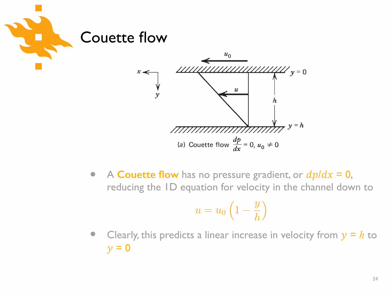
• A Couette flow has no pressure gradient, or *%/*# = 0, reducing the 1D equation for velocity in the channel down to

• Clearly, this predicts a linear increase in velocity from $ = � to $ = 0

24

u = u0

⇣1� y

h

⌘

Poiseuille flow

• Poiseuille flow is driven only by a pressure gradient in the channel with zero boundary velocities ("0 = 0), thus

• In a coordinate system with $ʹ at the middle of the channel we can say $ʹ = $ - �/2, which results in the relationship

25

u =1

2⌘

dp

dx

(y2 � hy)

u =1

2⌘

dp

dx

✓y

02 � h

2

4

◆

Application: Salt tectonics

!

!

!

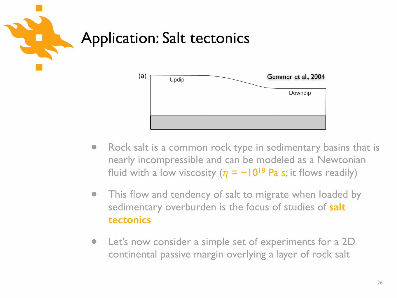
• Rock salt is a common rock type in sedimentary basins that is nearly incompressible and can be modeled as a Newtonian fluid with a low viscosity (! = ~1018 Pa s; it flows readily)!

• This flow and tendency of salt to migrate when loaded by sedimentary overburden is the focus of studies of salt tectonics!

• Let’s now consider a simple set of experiments for a 2D continental passive margin overlying a layer of rock salt

26

and initial velocity analytically and in the section‘Compar-ison of analytical and numerical results’ we compare theseresults with those from the numerical models.

Thin sheet approximation of the stabilityanalysis

Lehner (2000) uses local balance of stresses to predict in-itial deformation styles of systems with a viscous substrateoverlain by frictional-plastic sediments of laterally varyingthickness. In this section, we re-derive the Lehner (2000)stability criterion using balance of the horizontal bulkforces that act on the transition zonewhere the overburdenis thinning.We consider vertical plane-strain initial geo-metries, like those of Fig.1, inwhich the base is horizontaland the linear viscous layer has a uniform thickness be-neath a variable thickness frictional-plastic overburden.No consideration is given to theway inwhich the geometrywas created or to the ¢nite deformation. Consider the hor-izontal force balance of the overburden transition zoneoutlined by the thick line (Fig. 2). The upper surface isstress free and forces F1 and F2 result from the verticallyintegrated horizontal stresses in the frictional overburden.The di¡erential overburden load also induces a Poiseuille£ow in the viscous layer, which produces shear traction onthe base of the overburden resulting in the horizontalforce Fp.The overburden is stable against outward £ow inthe downdip direction when

F1 þ F2 þ Fp < 0 ð1Þusing the sign convention that forces directed to the rightare positive. In this case the forces, F1 and F2, are below

their respective extensional and contractional yield values.By introducing the yieldvalues ofF1andF2, Eqn. (1) can berewritten as the stability condition for outward £ow of theoverburden

F1e þ F2c þ Fp < 0 system is stable ð2aÞ

F1e þ F2c þ Fp < 0 system is unstable ð2bÞ

where F1e and F2c are the forces that result from limitingextensional and contractional horizontal stresses in theplastic overburden, above locations x1 and x2. The Mohr^Coulomb criterion is used to represent the cohesionlessfrictional-plastic behaviour of the overburden

txz ¼ szz % sxx ¼ &ðsxx þ szzÞ sinf ð3Þ

txz is the shear stress andf is the internal angle of friction.To estimate these limiting horizontal forces, we assumethat the principal stresses in the overburden are horizontal(sxx) andvertical (szz) and that szz is equal to the lithostaticpressure (small angle approach, Dahlen,1990), which yields

sxx ¼ %rgðhc þ hðxÞ % zÞ ð1& sinfÞð1& sinfÞ

ð4Þ

where r is the density, g is the gravitational accelerationand (hc1h(x)% z) is the depth.The resulting forces are

F1e ¼ %Z

h1

minðsxxÞ dz ¼12rg h21

ð1% sinfÞð1þ sinfÞ ð5aÞ

F2c ¼ %Z

h2

maxðsxxÞ dz ¼12rg h22

ð1þ sinfÞð1% sinfÞ

ð5bÞ

(note the di¡erent signs in the force expressions due to theopposite orientations of the outward normal vectors to thetwo surfaces onwhich the forces are acting).

To estimate the basal traction force, Fp, we assume thatthe topography changes slowly with position and thereforethat slopes are small.The thin sheet approximation (Lob-kovsky & Kerchman, 1991) then gives the distribution ofhorizontal velocities, vp, in the viscous substratum subjectto variations of lithostatic pressure as

vp ¼ % rg2Z

@hðxÞ@x

zðhc % zÞ ð6Þ

Fig.1. Deformation styles in systems where a frictional-plasticoverburden (white) of varying thickness overlies a viscoussubstratum (grey). (a) Stable overburden. A pressure-drivenPoiseuille £ow in the viscous channel dominates deformation.(b) Unstable overburden.The Couette £ow-induced overburdenvelocities are smaller than the Poiseuille £ow velocities in theviscous channel. (c) Unstable overburden. Couette £owdominates the deformation pattern.

Fig. 2. Horizontal forces acting on the overburden transitionzone (outlined by a thick solid line) when the model is stable.F1 and F2 are forces related to the horizontal stresses within theoverburden. Fp is the traction force caused by the Poiseuille £owin the viscous channel. h1 and h2 are the updip and downdipoverburden thicknesses and hc is the thickness of the salt.r is thedensity,f is the internal angle of friction and Z is the viscosity.

r 2004 Blackwell Publishing Ltd,Basin Research, 16, 199^218 201

Salt tectonics driven by differential sediment loading

Gemmer et al., 2004


!

!

!

• In this scenario, we might expect different flow behavior in the rock salt depending on the deformation of the overlying sediment!

• We predict Poiseuille flow when the sedimentary overburden is stable and does not move horizontally

27












ð4Þ


F1e ¼ %Z

h1



F2c ¼ %Z

h2



ð5bÞ



vp ¼ % rg2Z

@hðxÞ@x

zðhc % zÞ ð6Þ





Gemmer et al., 2004


!

!

!

• When the sedimentary overburden cannot support the lateral stress due to variations in its thickness, failure will occur in the sediments, leading to horizontal translation of the sediment!

• This produces a dominantly Couette-type of flow in the salt

28












ð4Þ


F1e ¼ %Z

h1



F2c ¼ %Z

h2



ð5bÞ



vp ¼ % rg2Z

@hðxÞ@x

zðhc % zÞ ð6Þ





Gemmer et al., 2004


!

!

!

• In nature, it is likely that salt flows in this type of environment involve both Couette and Poiseuille components, resulting in a velocity field that is a combination of both

29and initial velocity analytically and in the section‘Compar-ison of analytical and numerical results’ we compare theseresults with those from the numerical models.











ð4Þ


F1e ¼ %Z

h1



F2c ¼ %Z

h2



ð5bÞ



vp ¼ % rg2Z

@hðxÞ@x

zðhc % zÞ ð6Þ





Gemmer et al., 2004


30Gemmer et al., 2004

thick. For this model the basal traction caused by the £ow-ing viscous material is su⁄cient to cause overburdenyielding, and the system is characterised by a combinationof Poiseuille and Couette £ow. Figure 5c shows a modelwith a thin (1.5 km) downdip overburden. In this case, theCouette velocity caused by the unstable, moving overbur-den is signi¢cantly greater than the Poiseuille velocity anda linear velocity pro¢le develops in the viscous layer.Thusthe numerical model results conform to the conceptual£ow regimes illustrated in Fig.1.

COMPARISON OFANALYTICAL ANDNUMERICAL RESULTSStability results

The stability criterion de¢ned byEqn. (8) is shown as a so-lid curve (Fig. 6) as a function of the internal angle of fric-tion f and the downdip overburden thickness, h!2, for aconstant value of the updip overburden thickness,h!1 ¼ 4:5. For a given internal angle of friction, f a mini-mum value of h!2 is needed for the overburden to remainstable. For progressively higher internal angles of friction,the overburden strength increases and the h!2needed tokeep the overburden stable decreases.To test the response

of the ¢nite-element model against the stability criterion,we examine sets of models inwhich h!1 is held constant, andh!2 is varied for a given overburden strength f. Numericalmodel sets of this type span 514f4501 (Fig. 6) to yield asuite of model results for comparison with the non-di-mensional analytical stability criterion. The numericalmodel results are converted to the non-dimensional formusing hc and k as de¢ned in Eqn. (8).The results are codedaccording to the initial velocity pattern predicted for the¢rst 10 time steps (before signi¢cant changes in the geo-metry occur) (Fig. 6). The overall results show a goodagreement between the ¢nite-element models and theanalytically predicted stability criterion. This indicatesthat the numerical model is capable of calculating stressesand overburden stability associated with £ows caused bydi¡erential loading. It is not possible to determine the ab-solute accuracy of the numerical results from the compar-ison of the numerical model and the analytical predictionsbecause the analytical theory is itself approximate.

Initial velocities

A suite of similar numerical models was compared withthe analytical Couette velocity prediction of Eqn. (12). Forthese models, h!1 ¼ 4:5 and the internal angle of friction

Fig. 5. Velocities predicted by the numerical model. Arrows represent horizontal velocity vectors, the magnitude ofwhich is relative tothe scale in each frame. Light grey: Frictional-plastic overburden. Dark grey: viscous substratum. (a) Poiseuille-dominated £ow.(b) Combined Poiseuille and Couette £ow. (c) Couette-dominated £ow. Note in all three cases that £ow is restricted to the transitionzone.



Numerical model predictions for variable sediment strength

Asthenospheric counterflow

• One model for mantle flow is that the motion of lithospheric plates on the Earth’s surface produces a counterflow in the uppermost asthenosphere (upper ~100-200 km)!

• If we assume the plate is rigid and moving at velocity "0, and that the velocity at some depth $ = � must be zero, it is clear that the counterflow is opposite in direction to the plate motion in order to conserve mass

31


• Mathematically, we can state that aswhere �, is the thickness of the lithosphere and � is the thickness of the asthenosphere!

• If we insert our equation for 1D channel flow in the second term, we get

32

u0hL +

Z h

0u dy = 0

u0hL +h

3

12⌘

dp

dx

+u0h

2= 0


• If we now solve for the pressure gradient, we find

• And this can be inserted into the equation for 1D channel flow to get the predicted velocity profile for a counterflow

33

dp

dx

=12⌘u0

h

2

✓hL

h

+1

2

◆

u = u0

1� y

h+ 6

✓hL

h+

1

2

◆✓y2

h2� y

h

◆�


!

!

• Looking at this equation for a moment, what strikes you as perhaps somewhat surprising?

• Is there anything missing that you might expect to see?

34

u = u0

1� y

h+ 6

✓hL

h+

1

2

◆✓y2

h2� y

h

◆�

Kinematic viscosity and the Prandtl number

• We’ve dealt thus far with the dynamic viscosity !, but a similar quantity, the kinematic viscosity -, can be quite useful

• One reason this is useful is the units. - has units of m2 s-1, meaning it can be thought of as a diffusivity for momentum, much like ., the thermal diffusivity

35

⌫ =⌘

⇢

Kinematic viscosity and the Prandtl number

!

!

!

!

• The Prandtl number is the ratio of the kinematic viscosity to the thermal diffusivity, giving us a relationship between thermal diffusion and diffusion of momentum

• A fluid with a large Prandtl number will diffuse momentum more quickly than heat and the opposite is true for a fluid with a small Prandtl number

36

Pr ⌘ ⌫

414 Fluid Mechanics

Table 6.1 Transport Properties of Some Common Fluids at 15◦C andAtmospheric Pressure

Kinematic ThermalViscosity µ Viscosity ν Diffusivity κ Prandtl(Pa s) (m2 s−1) (m2 s−1) Number Pr

Air 1.78 × 10−5 1.45 × 10−5 2.02 × 10−5 0.72Water 1.14 × 10−3 1.14 × 10−6 1.40 × 10−7 8.1Mercury 1.58 × 10−3 1.16 × 10−7 4.2 × 10−6 0.028Ethyl alcohol 1.34 × 10−3 1.70 × 10−6 9.9 × 10−8 17.2Carbon tetrachloride 1.04 × 10−3 6.5 × 10−7 8.4 × 10−8 7.7Olive oil 0.099 1.08 × 10−4 9.2 × 10−8 1,170Glycerine 2.33 1.85 × 10−3 9.8 × 10−8 18,880

Newtonian fluid is the constant of proportionality between shear stress andstrain rate or velocity gradient. The more viscous the fluid, the larger thestress required to produce a given shear.

The viscosities of some common fluids are listed in Table 6–1. The SI unitof viscosity is the Pascal second (Pa s). The ratio µ/ρ (ρ is the density ofthe fluid) occurs frequently in fluid mechanics. It is known as the kinematicviscosity ν of a fluid

ν =µ

ρ. (6.2)

The quantity µ is the dynamic viscosity. The SI unit of kinematic viscosityis square meter per second (m2 s−1). The kinematic viscosity is a diffusivity,similar to the thermal diffusivity κ. While κ describes how heat diffuses bymolecular collisions, ν describes how momentum diffuses. The ratio of ν toκ is a dimensionless quantity known as the Prandtl number, Pr

Pr ≡ν

κ. (6.3)

A fluid with a small Prandtl number diffuses heat more rapidly than it doesmomentum; the reverse is true for a fluid with a large value of Pr. Table6–1 also lists the kinematic viscosities, thermal diffusivities, and Prandtlnumbers of a variety of fluids.

The flow in the channel in Figure 6–1 is determined by the equation ofmotion. This is a mathematical statement of the force balance on a layerof fluid of thickness δy and horizontal length l (see Figure 6–1). The netpressure force on the element in the x direction is

(p1 − p0) δy.

Hydraulic head

• Pressure drops in channels are often related to a hydraulic head

• The hydraulic head is the thickness (or height) of a fluid required to generate a hydrostatic pressure equal to %1 - %0, the pressure drop along the channel

37

H ⌘ (p1 � p0)

⇢g

Recap

• Fluid mechanics describes fluid motion based on the conservation of mass, momentum and energy!

!

• 1D channel flows can be divided into two fundamental types that relate to the conditions in the channel!

• Couette flow: Linear velocity gradient across channel, pressure gradient very small!

• Poiseuille flow: Parabolic velocity profile across channel, minimal displacement of channel walls

38

References

Gemmer, L., Ings, S. J., Medvedev, S., & Beaumont, C. (2004). Salt tectonics driven by differential sediment loading: stability analysis and finite-element experiments. Basin Research, 16(2), 199–218.

39

Basics of fluid mechanics - DPHU · Geodynamics .ﬁ/yliopisto Geodynamics Lecture 9 Basics of...

Documents

Transcript of Basics of fluid mechanics - DPHU · Geodynamics .ﬁ/yliopisto Geodynamics Lecture 9 Basics of...