-1

Basics and principles of particle image velocimetry (PIV) for mapping biogenic

and biologically relevant flows

Eize J. StamhuisDepartment of Marine Biology, University of Groningen, P.O. Box 31, 9750 AA Haren, The Netherlands;(e-mail: e.j.stamhuis@biol.rug.nl; phone: +31-50-3632078)

Received 9 September 2004; accepted in revised form 26 April 2005

Key words: Benthic boundary layer, BIOFLOW, Biogenic flows, Flow analysis, PIV

Abstract

Particle image velocimetry (PIV) has proven to be a very useful technique in mapping animal-generatedflows or flow patterns relevant to biota. Here, theoretical background is provided and experimental detailsof 2-dimensional digital PIV are explained for mapping flow produced by or relevant to aquatic biota. Themain principles are clarified in sections on flow types, seeding, illumination, imaging, repetitive correlationanalysis, post-processing and result interpretation, with reference to experimental situations. Examplesfrom the benthic environment, namely, on filter feeding in barnacles and in bivalves, illustrate what theexperiments comprise and what the results look like. Finally, alternative particle imaging flow analysistechniques are discussed briefly in the context of mapping biogenic and biologically relevant flows.

Introduction

Particle image velocimetry (PIV) has been devel-oped from the early 1980’s onwards to map com-plete flow fields instantaneously (Adrian 1991).The novelty and great advantage of PIV are that itdelivers high resolution flow velocity vectorinformation of a whole plane in the flow in onetime. All other methods known until the 1980’sdelivered point values, or low resolution vectordiagrams of whole planes after repeating theexperiment several times. Consequently, PIV hasgiven new impulse to fluid dynamics research, inparticular at unsteady flows that were difficult tomap instantly beforehand (Raffel et al. 1998).

PIV has been developed in the fields of funda-mental and applied fluid dynamics research andmechanical engineering. It has therefore mainlybeen used to study experimentally induced flows,such as water flow in confined areas or aroundstreamlined objects, air flow around wing profiles

and plane models, etc. (Adrian 1991; Stanislaset al. 2000). Since 1993, PIV has been applied tobiogenic or biologically important flows, usingsystems that were either developed for this purpose(e.g. Stamhuis and Videler 1995; Muller et al.1997) or adapted or tuned to the particular cir-cumstances (e.g. Drucker and Lauder 1999; Zirbelet al. 2000). Due to its non-intrusive character,PIV can be characterised as an ideal tool forstudying animal-generated flows, restricting dis-turbances and thereby non-natural behaviour to aminimum.

For the benthic zone, information on methodsfor flow studies, on flow facilities and on resultsare being exchanged within the European BIO-FLOW network. This paper contributes to thisexchange by explaining the basics and principlesof PIV, being one of the more recently developedflow mapping methods that can well be applied tostudy flows in the benthic zone. It will focus on 2-dimensional (planar) PIV and is geared to scien-

Aquatic Ecology (2006) 40:463–479 � Springer 2006

DOI 10.1007/s10452-005-6567-z

tists that have no real experience with PIV and donot have a degree in physics, fluid dynamics ormathematics. For detailed background informa-tion on PIV, the following references may provevaluable: Particle Image Velocimetry, a practicalguide (Raffel et al. 1998), Particle Image Veloci-metry (Hinsch 1993), and the Special Issue onPIV of Measurement Science and Technology,Volume 8 Nr 12 (Jones 1997), in particular thefirst paper in this volume, on the Fundamentals ofDigital PIV (Westerweel 1997). Digital PIV, the-ory and application (Westerweel 1993) is recom-mended for the theoretical backgrounds ofDigital PIV (DPIV). Details on DPIV applied toanimal generated flows and on the specific prob-lems that one can run into when working withanimals in flow studies, can be found in Stamhuisand Videler (1995), and Stamhuis et al. (2002).The nature of flow phenomena around biota ingeneral and the basic relationships betweenorganisms and their fluid environment are verywell explained by Steven Vogel in his book Life inMoving Fluids, the physical biology of flow (Vogel1994) which is recommended for basic back-ground reading.

The following subjects will be covered succes-sively: (1) 2D-PIV in a nut-shell, describing what2D-PIV basically comes down to; (2) The basicsand principles of 2D-PIV, with explanatory sec-tions on every step when applying 2D-PIV; (3)Biological examples, shortly covering two exam-ples from our studies on biogenic flows, (4) OtherPIV-techniques, with an overview and discussionof recent developments such as Micro-PIV, Ste-reo-PIV, Holographic PIV, Super Resolution PIVand 3D Particle Tracking Velocimetry (3D-PTV);

and (5) Conclusion. The treatment of sections 1,2 and 3 is based mainly on of the author’s ownexperience with reference to the literature andsection 4 is a brief overview of the relevant lit-erature.

PIV in a nut-shell

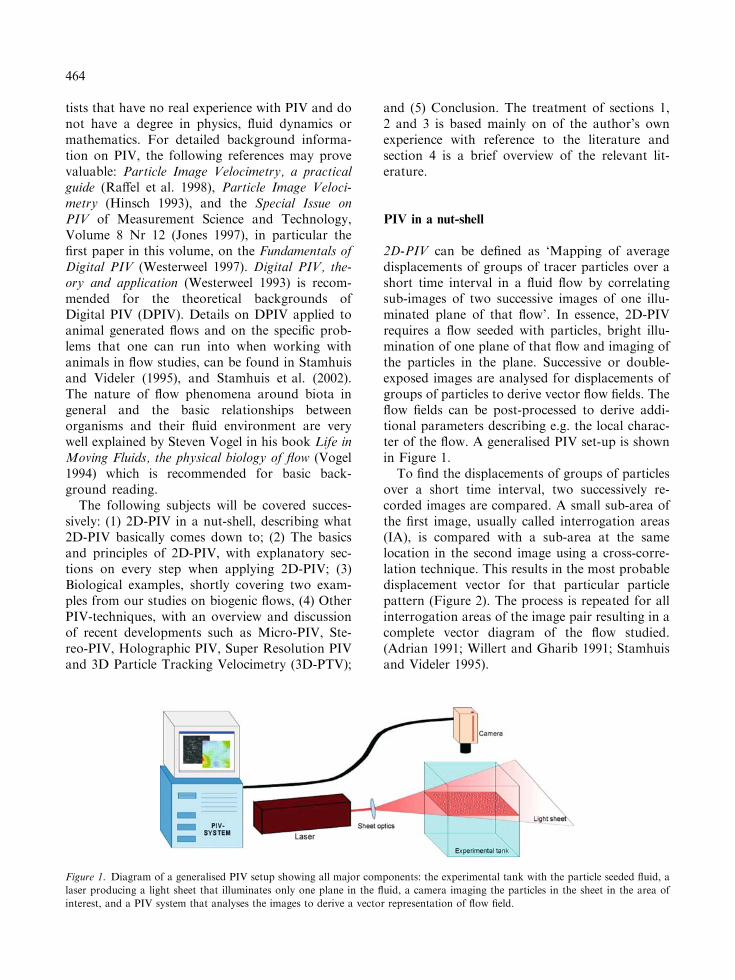
2D-PIV can be defined as ‘Mapping of averagedisplacements of groups of tracer particles over ashort time interval in a fluid flow by correlatingsub-images of two successive images of one illu-minated plane of that flow’. In essence, 2D-PIVrequires a flow seeded with particles, bright illu-mination of one plane of that flow and imaging ofthe particles in the plane. Successive or double-exposed images are analysed for displacements ofgroups of particles to derive vector flow fields. Theflow fields can be post-processed to derive addi-tional parameters describing e.g. the local charac-ter of the flow. A generalised PIV set-up is shownin Figure 1.

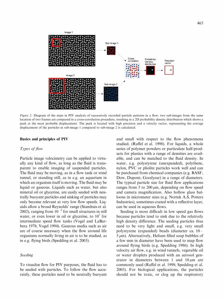
To find the displacements of groups of particlesover a short time interval, two successively re-corded images are compared. A small sub-area ofthe first image, usually called interrogation areas(IA), is compared with a sub-area at the samelocation in the second image using a cross-corre-lation technique. This results in the most probabledisplacement vector for that particular particlepattern (Figure 2). The process is repeated for allinterrogation areas of the image pair resulting in acomplete vector diagram of the flow studied.(Adrian 1991; Willert and Gharib 1991; Stamhuisand Videler 1995).

Figure 1. Diagram of a generalised PIV setup showing all major components: the experimental tank with the particle seeded fluid, a

laser producing a light sheet that illuminates only one plane in the fluid, a camera imaging the particles in the sheet in the area of

interest, and a PIV system that analyses the images to derive a vector representation of flow field.

464

Basics and principles of PIV

Types of flow

Particle image velocimetry can be applied to virtu-ally any kind of flow, as long as the fluid is trans-parent to enable imaging of suspended particles.The fluid may be moving, as in a flow tank or windtunnel, or standing still, as in e.g. an aquarium inwhich an organism itself is moving. The fluid may beliquid or gaseous. Liquids such as water, but alsomineral oil or glycerine, are easily seeded with neu-trally buoyant particles and sinking of particles mayonly become relevant at very low flow speeds. Liq-uids allow a broad Reynolds’ range (Stamhuis et al.2002), ranging from 10�2 for small structures in stillwater, or even lower in oil or glycerine, to 107 forintermediate speed flow tanks (Vogel and LaBar-bera 1978; Vogel 1994). Gaseous media such as airare of course necessary when the flow around lifeorganisms normally living in air is to be studied, asin e.g. flying birds (Spedding et al. 2003).

Seeding

To visualise flow for PIV purposes, the fluid has tobe seeded with particles. To follow the flow accu-rately, these particles need to be neutrally buoyant

and small with respect to the flow phenomenastudied, (Raffel et al. 1998). For liquids, a wholeseries of polymer powders or particulate half-prod-ucts for plastics with a range of densities are avail-able, and can be matched to the fluid density. Inwater, e.g. polystyrene (unexpanded), polythene,nylon, PVC or pliolite particles work well and canbe purchased from chemical companies (e.g. BASF,Dow, Dupont, Goodyear) in a range of diameters.The typical particle size for fluid flow applicationsranges from 5 to 200lm, depending on flow speedand camera magnification. Also hollow glass bal-loons in micrometer sizes (e.g. Nortek A.S, PottersIndustries), sometimes coated with a reflective layer,can be used in aqueous flows.

Seeding is more difficult in low speed gas flowsbecause particles tend to sink due to the relativelyhigh density difference. The seeding particles thusneed to be very light and small, e.g. very smallpolystyrene (expanded) beads (diameter ca. 10 –5 lm). Alternatively, Helium filled soap bubbles ofa few mm in diameter have been used to map flowaround flying birds (e.g. Spedding 1986). In highvelocity air flow, e.g. in wind tunnels, vegetable oilor water droplets produced with an aerosol gen-erator in diameters between 1 and 10 lm arecommonly used (Raffel et al. 1998; Spedding et al.2003). For biological applications, the particlesshould not be toxic, or clog up the respiratory

Figure 2. Diagram of the steps in PIV analysis of successively recorded particle patterns in a flow: two sub-images from the same

location of two frames are compared in a cross-correlation procedure, resulting in a 2D probability density distribution which shows a

peak at the most probable displacement. The peak is located with high precision and a velocity vector, representing the average

displacement of the particles in sub-image 1 compared to sub-image 2 is calculated.

465

structures of the organisms involved (see alsoStamhuis et al. 2002). In all cases the particlesshould preferably be highly reflective, to yieldgood particle images on the PIV recordings.

Illumination

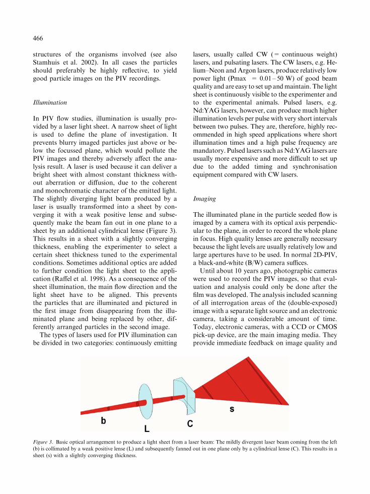
In PIV flow studies, illumination is usually pro-vided by a laser light sheet. A narrow sheet of lightis used to define the plane of investigation. Itprevents blurry imaged particles just above or be-low the focussed plane, which would pollute thePIV images and thereby adversely affect the ana-lysis result. A laser is used because it can deliver abright sheet with almost constant thickness with-out aberration or diffusion, due to the coherentand monochromatic character of the emitted light.The slightly diverging light beam produced by alaser is usually transformed into a sheet by con-verging it with a weak positive lense and subse-quently make the beam fan out in one plane to asheet by an additional cylindrical lense (Figure 3).This results in a sheet with a slightly convergingthickness, enabling the experimenter to select acertain sheet thickness tuned to the experimentalconditions. Sometimes additional optics are addedto further condition the light sheet to the appli-cation (Raffel et al. 1998). As a consequence of thesheet illumination, the main flow direction and thelight sheet have to be aligned. This preventsthe particles that are illuminated and pictured inthe first image from disappearing from the illu-minated plane and being replaced by other, dif-ferently arranged particles in the second image.

The types of lasers used for PIV illumination canbe divided in two categories: continuously emitting

lasers, usually called CW (= continuous weight)lasers, and pulsating lasers. The CW lasers, e.g. He-lium–Neon and Argon lasers, produce relatively lowpower light (Pmax = 0.01– 50 W) of good beamquality and are easy to set up andmaintain. The lightsheet is continuously visible to the experimenter andto the experimental animals. Pulsed lasers, e.g.Nd:YAG lasers, however, can produce much higherillumination levels per pulse with very short intervalsbetween two pulses. They are, therefore, highly rec-ommended in high speed applications where shortillumination times and a high pulse frequency aremandatory. Pulsed lasers such asNd:YAG lasers areusually more expensive and more difficult to set updue to the added timing and synchronisationequipment compared with CW lasers.

Imaging

The illuminated plane in the particle seeded flow isimaged by a camera with its optical axis perpendic-ular to the plane, in order to record the whole planein focus. High quality lenses are generally necessarybecause the light levels are usually relatively low andlarge apertures have to be used. In normal 2D-PIV,a black-and-white (B/W) camera suffices.

Until about 10 years ago, photographic cameraswere used to record the PIV images, so that eval-uation and analysis could only be done after thefilm was developed. The analysis included scanningof all interrogation areas of the (double-exposed)image with a separate light source and an electroniccamera, taking a considerable amount of time.Today, electronic cameras, with a CCD or CMOSpick-up device, are the main imaging media. Theyprovide immediate feedback on image quality and

Figure 3. Basic optical arrangement to produce a light sheet from a laser beam: The mildly divergent laser beam coming from the left

(b) is collimated by a weak positive lense (L) and subsequently fanned out in one plane only by a cylindrical lense (C). This results in a

sheet (s) with a slightly converging thickness.

466

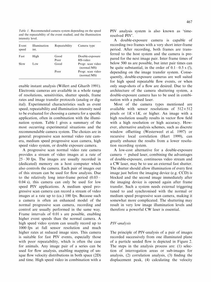
enable instant analysis (Willert and Gharib 1991).Electronic cameras are available in a whole rangeof resolutions, sensitivities, shutter speeds, framerates and image transfer protocols (analog or dig-ital). Experimental characteristics such as eventspeed, repeatability and illumination intensity needto be evaluated for choosing a camera for a specificapplication, often in combination with the illumi-nation system. Table 1 gives a summary of themost occurring experimental situations and therecommendable camera system. The choices are ingeneral: progressive scan normal video rate cam-era, medium speed progressive scan camera, highspeed video system, or double exposure camera.

A progressive scan normal video rate cameraprovides a stream of video images at a rate of25 – 30 fps. The images are usually recorded in(dedicated) memory on a host computer whichalso controls the camera. Each pair of images outof this stream can be used for flow analysis. Dueto the relatively long inter-frame period (0.03 –0.04 s), this camera can only be used for lowspeed PIV applications. A medium speed pro-gressive scan camera can record a stream of videoimages at a rate up to (ca.) 100 fps. Because sucha camera is often an enhanced model of thenormal progressive scan camera, recording andcontrol are usually performed in the same way.Frame intervals of 0.01 s are possible, enablinghigher event speeds than the normal camera. Ahigh speed video system can usually record up to1000 fps at full sensor resolution and muchhigher rates at reduced image sizes. This camerais suitable for fast PIV events, especially thosewith poor repeatability, which is often the casefor animals. Any image pair of a series can beused for flow analysis, enabling mapping of un-ique flow velocity distributions in both space (2D)and time. High speed video in combination with a

PIV analysis system is also known as ‘time-resolved PIV’.

A double-exposure camera is capable ofrecording two frames with a very short inter-frameperiod. After recording, both frames are trans-ferred to the host system and the camera is pre-pared for the next image pair. Inter frame times ofbelow 500 ns are possible, but inter pair times canbe quite substantial, in the order of 0.1 – 0.5 s (!),depending on the image transfer system. Conse-quently, double-exposure cameras are well suitedfor high speed repeatable flow events, or whenonly snap-shots of a flow are desired. Due to thearchitecture of the camera shuttering system, adouble-exposure camera has to be used in combi-nation with a pulsed laser.

Most of the camera types mentioned areavailable with sensor resolutions of 512 · 512pixels or 1K · 1K, or higher. An image with ahigh resolution usually results in vector flow fieldwith a high resolution or high accuracy. How-ever, alternative analysis schemes, such as discretewindow offsetting (Westerweel et al. 1997) orrecursive local correlation (Hart 1999), cangreatly enhance the results from a lower resolu-tion recording system.

A low-cost alternative for a double-exposurecamera + pulsed laser, combining the advantagesof double-exposure, continuous video stream anda CW laser, may be to use an external fast shutter.The shutter should allow illumination of every firstimage just before the imaging device (e.g. CCD) isblocked and the second image immediately afterthe imaging device is opened again after frametransfer. Such a system needs external triggeringtuned to and synchronised with the normal ormedium speed progressive scan camera, making itsomewhat more complicated. The shuttering mayresult in very low image illumination levels andtherefore a powerful CW laser is essential.

PIV-analysis

The principle of PIV-analysis of a pair of imagesrecorded successively from one illuminated planeof a particle seeded flow is depicted in Figure 2.The steps in the analysis process are: (1) selec-tion of interrogation areas or sub-images foranalysis, (2) correlation analysis, (3) finding thedisplacement peak, (4) calculating the velocity

Table 1. Recommended camera system depending on the speed

and the repeatability of the event studied, and the illumination

intensity level.

Event

speed

Illumination

int.

Repeatability Camera type

Fast High Good Double-exposure

Poor HS-video

Slow Low Good Progr. scan video

(normal/MS)

Poor Progr. scan video

(normal/MS)

467

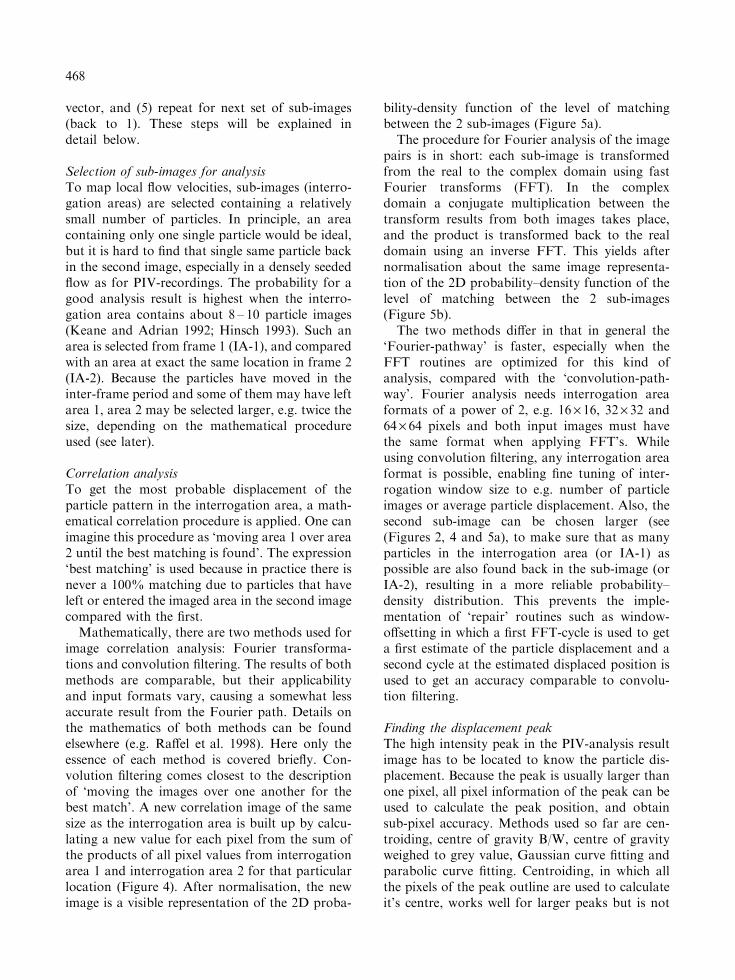
vector, and (5) repeat for next set of sub-images(back to 1). These steps will be explained indetail below.

Selection of sub-images for analysisTo map local flow velocities, sub-images (interro-gation areas) are selected containing a relativelysmall number of particles. In principle, an areacontaining only one single particle would be ideal,but it is hard to find that single same particle backin the second image, especially in a densely seededflow as for PIV-recordings. The probability for agood analysis result is highest when the interro-gation area contains about 8 – 10 particle images(Keane and Adrian 1992; Hinsch 1993). Such anarea is selected from frame 1 (IA-1), and comparedwith an area at exact the same location in frame 2(IA-2). Because the particles have moved in theinter-frame period and some of them may have leftarea 1, area 2 may be selected larger, e.g. twice thesize, depending on the mathematical procedureused (see later).

Correlation analysisTo get the most probable displacement of theparticle pattern in the interrogation area, a math-ematical correlation procedure is applied. One canimagine this procedure as ‘moving area 1 over area2 until the best matching is found’. The expression‘best matching’ is used because in practice there isnever a 100% matching due to particles that haveleft or entered the imaged area in the second imagecompared with the first.

Mathematically, there are two methods used forimage correlation analysis: Fourier transforma-tions and convolution filtering. The results of bothmethods are comparable, but their applicabilityand input formats vary, causing a somewhat lessaccurate result from the Fourier path. Details onthe mathematics of both methods can be foundelsewhere (e.g. Raffel et al. 1998). Here only theessence of each method is covered briefly. Con-volution filtering comes closest to the descriptionof ‘moving the images over one another for thebest match’. A new correlation image of the samesize as the interrogation area is built up by calcu-lating a new value for each pixel from the sum ofthe products of all pixel values from interrogationarea 1 and interrogation area 2 for that particularlocation (Figure 4). After normalisation, the newimage is a visible representation of the 2D proba-

bility-density function of the level of matchingbetween the 2 sub-images (Figure 5a).

The procedure for Fourier analysis of the imagepairs is in short: each sub-image is transformedfrom the real to the complex domain using fastFourier transforms (FFT). In the complexdomain a conjugate multiplication between thetransform results from both images takes place,and the product is transformed back to the realdomain using an inverse FFT. This yields afternormalisation about the same image representa-tion of the 2D probability–density function of thelevel of matching between the 2 sub-images(Figure 5b).

The two methods differ in that in general the‘Fourier-pathway’ is faster, especially when theFFT routines are optimized for this kind ofanalysis, compared with the ‘convolution-path-way’. Fourier analysis needs interrogation areaformats of a power of 2, e.g. 16 · 16, 32 · 32 and64 · 64 pixels and both input images must havethe same format when applying FFT’s. Whileusing convolution filtering, any interrogation areaformat is possible, enabling fine tuning of inter-rogation window size to e.g. number of particleimages or average particle displacement. Also, thesecond sub-image can be chosen larger (see(Figures 2, 4 and 5a), to make sure that as manyparticles in the interrogation area (or IA-1) aspossible are also found back in the sub-image (orIA-2), resulting in a more reliable probability–density distribution. This prevents the imple-mentation of ‘repair’ routines such as window-offsetting in which a first FFT-cycle is used to geta first estimate of the particle displacement and asecond cycle at the estimated displaced position isused to get an accuracy comparable to convolu-tion filtering.

Finding the displacement peakThe high intensity peak in the PIV-analysis resultimage has to be located to know the particle dis-placement. Because the peak is usually larger thanone pixel, all pixel information of the peak can beused to calculate the peak position, and obtainsub-pixel accuracy. Methods used so far are cen-troiding, centre of gravity B/W, centre of gravityweighed to grey value, Gaussian curve fitting andparabolic curve fitting. Centroiding, in which allthe pixels of the peak outline are used to calculateit’s centre, works well for larger peaks but is not

468

very accurate for small ones, and the same is truefor calculation of the centre of gravity B/W(=after thresholding). Calculation of the centre ofgravity weighed to grey value, in which lighterpixels contribute more than darker ones, givesgood and accurate results for average size peaks (3pixels diameter) and even better for larger peaks.Gaussian and parabolic curve fitting work welland accurate on average size peaks (3 pixels) butare less reliable on smaller or larger peaks.Depending on the peak size and the method used,accuracies of less than one tenth of a pixel arepossible. With displacements of 3 pixels or more, aconfidence level of much higher than 95% can thusbe achieved.

Calculating velocity vectorsThe displacement information in pixels is trans-lated to real world units (metres or millimetres)after calibration. Subsequently, velocity vectorsare calculated by dividing the calibrated displace-ments by the inter-frame or inter-pulse time. Theresulting vectors can each be represented by ui andvi, being the components in X- and Y-direction of

the ith vector, respectively, or by a magnitude, andan angle with the horizontal with respect to adefined origin.

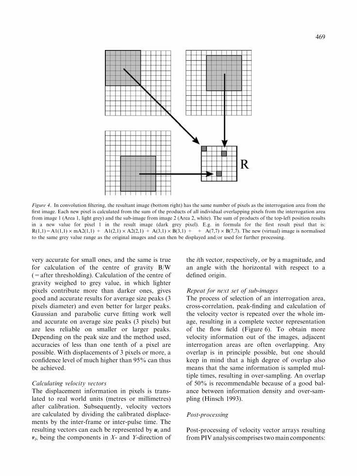
Repeat for next set of sub-imagesThe process of selection of an interrogation area,cross-correlation, peak-finding and calculation ofthe velocity vector is repeated over the whole im-age, resulting in a complete vector representationof the flow field (Figure 6). To obtain morevelocity information out of the images, adjacentinterrogation areas are often overlapping. Anyoverlap is in principle possible, but one shouldkeep in mind that a high degree of overlap alsomeans that the same information is sampled mul-tiple times, resulting in over-sampling. An overlapof 50% is recommendable because of a good bal-ance between information density and over-sam-pling (Hinsch 1993).

Post-processing

Post-processing of velocity vector arrays resultingfromPIVanalysis comprises twomain components:

Figure 4. In convolution filtering, the resultant image (bottom right) has the same number of pixels as the interrogation area from the

first image. Each new pixel is calculated from the sum of the products of all individual overlapping pixels from the interrogation area

from image 1 (Area 1, light grey) and the sub-image from image 2 (Area 2, white). The sum of products of the top-left position results

in a new value for pixel 1 in the result image (dark grey pixel). E.g. in formula for the first result pixel that is:

R(1,1)=A1(1,1) · mA2(1,1) + A1(2,1) · A2(2,1) + A(3,1) · B(3,1) + Æ + A(7,7) · B(7,7). The new (virtual) image is normalised

to the same grey value range as the original images and can then be displayed and/or used for further processing.

469

(1) data-validation and replacement of erroneousvectors, and (2) analysis and visualisation of veloc-ity gradients. They are both essential to get reliableand well-understandable results that help to quan-tify, comprehend and interpret the flow phenomenastudied, the ultimate goal of a PIV flow study.

Data validation and error correctionThe resultant vector set of automated PIV analysisoften includes a certain number of incorrect vec-tors that are usually obvious in the vector diagram.This type of erroneous vectors are usually causedby imperfections in the input images, caused

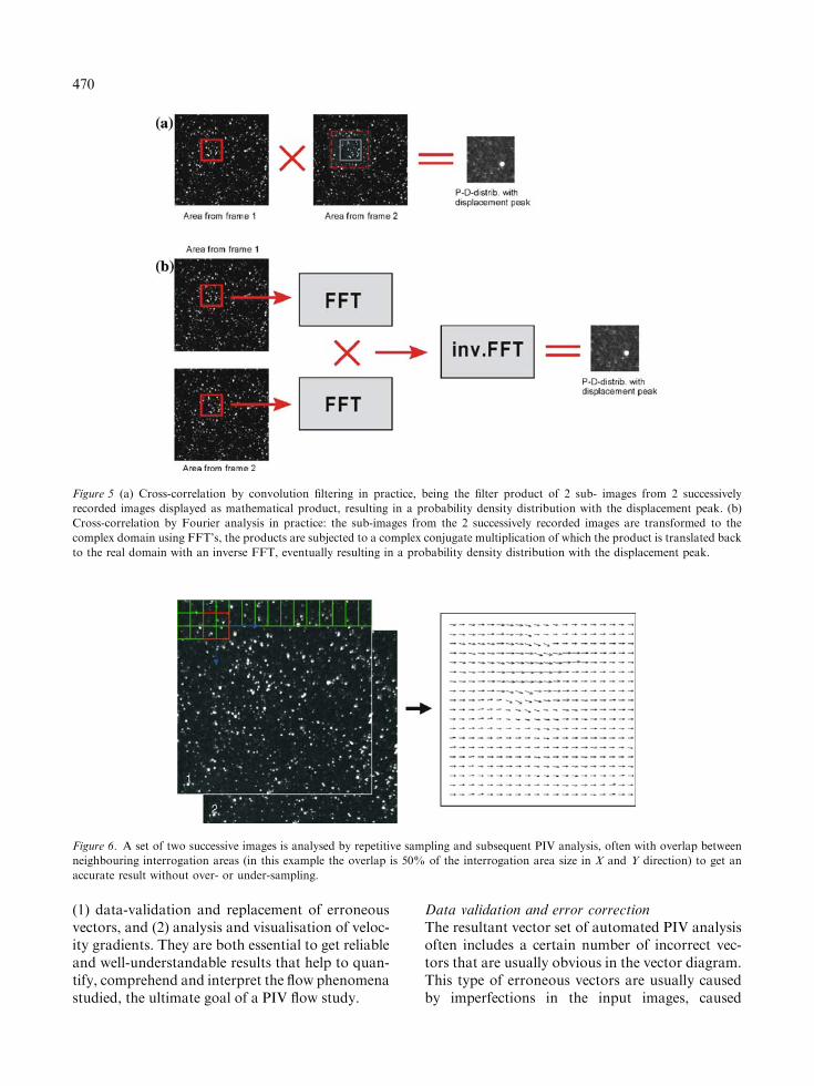
Figure 5 (a) Cross-correlation by convolution filtering in practice, being the filter product of 2 sub- images from 2 successively

recorded images displayed as mathematical product, resulting in a probability density distribution with the displacement peak. (b)

Cross-correlation by Fourier analysis in practice: the sub-images from the 2 successively recorded images are transformed to the

complex domain using FFT’s, the products are subjected to a complex conjugate multiplication of which the product is translated back

to the real domain with an inverse FFT, eventually resulting in a probability density distribution with the displacement peak.

Figure 6. A set of two successive images is analysed by repetitive sampling and subsequent PIV analysis, often with overlap between

neighbouring interrogation areas (in this example the overlap is 50% of the interrogation area size in X and Y direction) to get an

accurate result without over- or under-sampling.

470

mainly by local variations in seeding density, localover-illumination due to an object or wall in thelight sheet, strong out-of-plane-flow, local lowillumination close to the image borders, or crip-pled interrogation areas next to the image border.These problems cause lack of correlation in thenormal way, and a background (lower) peak isthen recognized as if it were the displacementpeak, resulting in an erroneous vector. Incorrectvectors usually stand out clearly with respect tosurrounding vectors, due to their different orien-tation and often different – read ‘much higher’ –magnitude (Figure 7a). This enables relatively easyrecognition to the observer as well as to anyautomated validation routine. Automated valida-tion routines usually compare every vector withthe surrounding one’s in e.g. a 3 · 3 matrix, anduse statistical parameters (e.g. the standard devi-ation or a histogram distribution function) or fluiddynamical parameters (e.g. vorticity or divergence)to discriminate between correct and erroneousvectors. The details of some of these validationprocedures are discussed elsewhere (e.g. Raffelet al. 1998). Sometimes, especially close to theimage border or when erroneous vectors show upin clusters, manual removal is necessary becauseautomated validation does not work due to lack ofreliable neighbours. This has to be done with greatcare, of course, and often needs an experiencedevaluator.

Once the incorrect vectors are recognized andremoved, empty places should preferably be filledby new vectors for continuous calculation of localderivatives and gradient parameters (see later).The new vector should represent the local flowvelocity as close as possible. The most commonway to do this is by 2D interpolation (Figure 7b).Although simple linear or polynomial interpola-tion yields reasonable results, the best and alsoprincipally the most reliable results have beenobtained with 2D cubic natural spline interpola-tion (Spedding and Rignot 1993; Stamhuis andVideler 1995). Cubic natural spline fits leave theoriginal neighbouring data unaffected and find themissing points according to ‘the most fluent line orplane’, i.e. with minimisation of the local curvature(second derivative). In non-compressible or sub-sonic compressible fluids, gradients are hardly eversudden, which illustrates why spline fits give thebest results. But even in shock waves in transonicflow, spline interpolation may perform very well.

Analysis and visualisation of velocity gradientsThe vector flow field resulting from the PIV anal-ysis and validation + interpolation proceduregives an enormous amount of information on localvelocity and direction of the flow. Sometimes it isdifficult to see the actual flow phenomena in thevector diagrams. Rotationality, for example, maybe masked by the overall flow speed, and so may beother gradients. A first tool to reveal hidden flowstructures is to subtract the average or backgroundflow from all vectors. This is often done whenstudying the flow phenomena caused by a still ormoving object, e.g. a wing section, in a flow tank orwind tunnel (Figure 7c vs. b). Additionally, thevelocity magnitude (absolute or relative) shown asa colour code superimposed on the vector diagramis also quite revealing (Figure 7d).

To visualise other gradients in the flow, anumber of parameters can be derived, of whichvorticity, rate of shear, rate of strain, divergenceand a vortex locator are most common and mostclarifying. These parameters are calculated fromthe local velocity derivatives (see Table 2) (Voll-mers et al. 1983; Lighthill 1986; Stamhuis andVideler 1995; Vollmers 2001). Two of them areillustrated in Figure 7e and f, showing the same jetpulse with accompanying circular flow areas(without background flow) as in Figure 7b, butnow with visualisation of the vorticity (Figure 7e)and the vortex cores (Figure 7f) through colourcoding. The rate of shear often helps to assess thevelocity profiles and pressure/force distributionsclose to objects or walls. The rate of strain in-dicates acceleration or decelerations of the flow.High strain rates in a 2D analysis are often in-dicative for a significant 3D flow component,which can be checked with the divergence. Becausethey are computed from the velocity derivatives,these parameters are insensitive to masking effectsof a high average flow speed or background flow.This makes them very useful in revealing the realbut sometimes visually hidden flow morphology,e.g. as in turbulence in high speed flows or im-pinging jets.

The distribution of vorticity and other derivedparameters give insight in the relative importanceand the distributions of velocity gradients in theflow field. That is above all necessary to assess andunderstand the morphology of the flow phenom-ena studied. Moreover, velocity vectors and de-rived parameters can be used for further

471

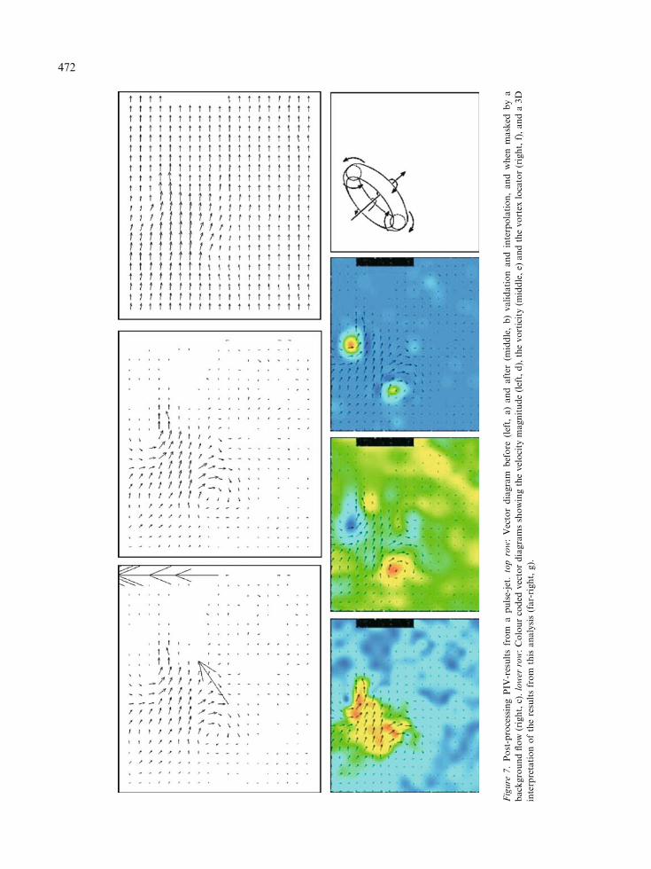
Figure

7.Post-processingPIV

-resultsfrom

apulse-jet.

toprow:Vectordiagram

before

(left,

a)andafter

(middle,b)validationandinterpolation,andwhen

masked

bya

backgroundflow

(right,c).lower

row:Colourcoded

vectordiagramsshowingthevelocity

magnitude(left,d),thevorticity(m

iddle,e)

andthevortex

locator(right,f),anda3D

interpretationoftheresultsfrom

thisanalysis(far-right,g).

472

processing or comparison, e.g. between successiveanalyses, between comparable setups, or to vali-date theoretical predictions.

Interpretation

To fully understand PIV results, proper interpre-tation is essential. A first challenge in interpreting2D PIV results (and of other types of PIV) is thatwe are basically looking at one 2D plane or onecross-section of a 3D flow phenomenon. On top ofthat, the flow pattern may be changing in time,which adds an extra dimension to our problem.For example, the mass of water travelling from theupper-left corner towards lower-right with itsneighbouring elevated vorticity areas as displayedin Figure 7a–f is in fact a cross-section of a jetpulse with accompanying vortex ring (Figure 7g).The exact shape and morphology of the jet + ringcombination can only be found when using a real3D visualisation technique or when repeating theexperiment and making a series of parallel andperpendicular cross sections. That may not alwaysbe possible, especially when working with biota.

For a good interpretation a good backgroundknowledge of the fluid dynamics involved, andexperience are important. The first of these twocan be found in fluid dynamics text books and inthe literature. Experience can only be built up bydirectly working with the technique. When study-ing 3D free flow structures, flows close to objectsor boundaries, sudden gradients, etc., one shouldbe aware of the three-dimensionality of the flowand know the limitations of 2D representations.

Examples from Biology

The application of 2D-DPIV to animal generatedflows is illustrated with two examples, one on acorn

barnacle filter feeding and one on filter feeding infour different bivalve species. All these animals arebenthic and were chosen because of the emphasis ofthe BIOFLOW network on benthic flow phenom-ena. These experiments serve as examples here, andthe results will be discussed only briefly becausethat is not in the scope of this paper.

The normal habitat of benthic animals is oftendominated by the external flow regime (waves andtides), but these animals may also generate theirown flow phenomena. Here we concentrate on theflow patterns generated by the animals themselves,with some detail on the PIV setup, recording andanalysis (for details see Stamhuis et al. 2002;Stamhuis and Vos in prep.). All PIV analyses wereperformed using SWIFT 4.0 (Dutch Vision Sys-tems), a commercially available package derivedfrom the system originally developed in our la-boratory, using convolution filtering for the cross-correlation analysis. Illumination was provided bya red CW Krypton laser at a wavelength of647 nm (Pmax = 1 W), delivered as a sheet at therecordable area through an armed glass fibre and alight sheet probe. The probe allows adjustment ofthe sheet thickness in the range 0.1–5 mm.

Acorn barnacle filter feeding

Acorn barnacles from the North Sea area arerelatively small crustaceans living in protectivecalcareous tests, that colonize hard substratessuch as rocks, dikes, breakwaters and bivalveshells. They have relatively long leg-like structurescalled cirri that can be extended and sweptthrough the water to filter it for food, such asdetritus particles and small planktonic organisms.Due to the small size of the cirri (lengths around6 mm, diameter <0.2 mm) and their low beatfrequencies (around 1 beat/s), they are confronted

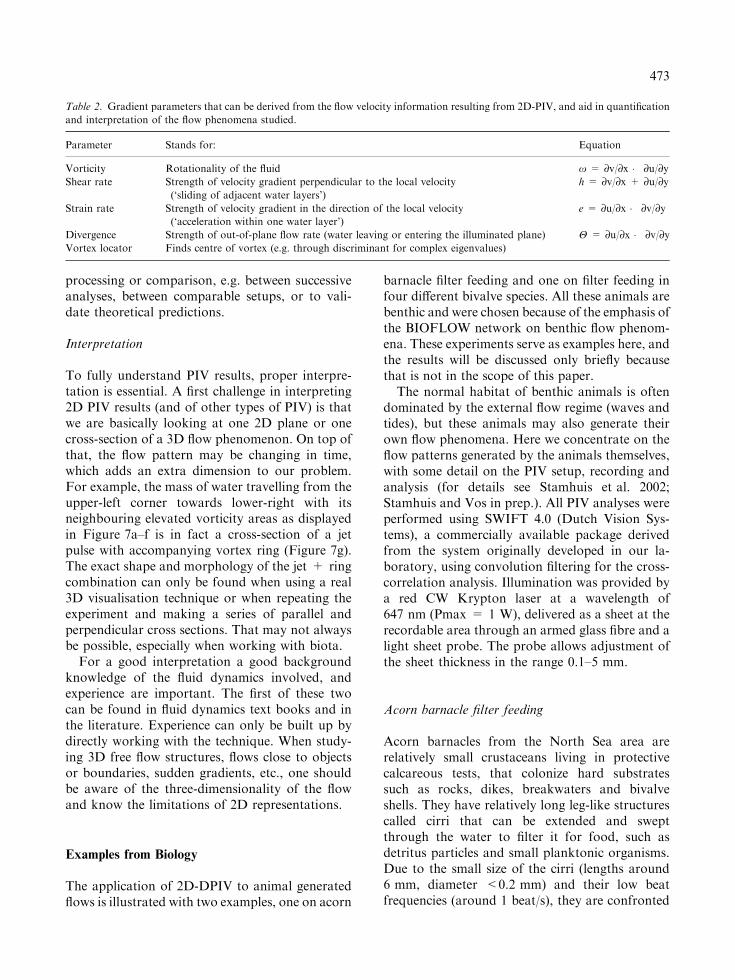
Table 2. Gradient parameters that can be derived from the flow velocity information resulting from 2D-PIV, and aid in quantification

and interpretation of the flow phenomena studied.

Parameter Stands for: Equation

Vorticity Rotationality of the fluid x = ¶v/¶x � ¶u/¶yShear rate Strength of velocity gradient perpendicular to the local velocity

(‘sliding of adjacent water layers’)

h = ¶v/¶x + ¶u/¶y

Strain rate Strength of velocity gradient in the direction of the local velocity

(‘acceleration within one water layer’)

e = ¶u/¶x � ¶v/¶y

Divergence Strength of out-of-plane flow rate (water leaving or entering the illuminated plane) H = ¶u/¶x � ¶v/¶yVortex locator Finds centre of vortex (e.g. through discriminant for complex eigenvalues)

473

with viscous as well as inertial flow aspects. Thebarnacles used in the experiments (Balanuscrenatus) are only actively beating at very lowambient flow velocities, and were studied whilefeeding in still water.

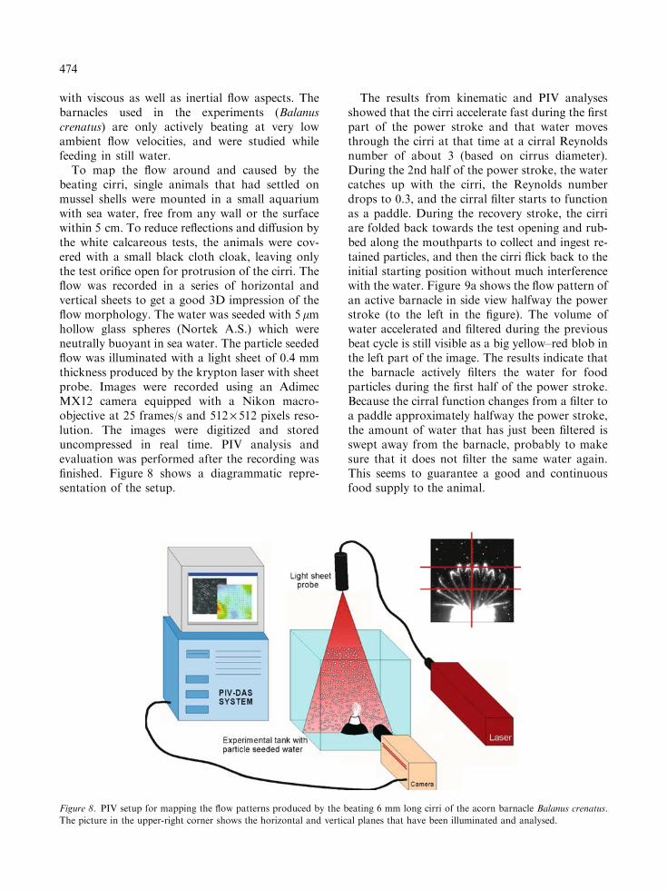
To map the flow around and caused by thebeating cirri, single animals that had settled onmussel shells were mounted in a small aquariumwith sea water, free from any wall or the surfacewithin 5 cm. To reduce reflections and diffusion bythe white calcareous tests, the animals were cov-ered with a small black cloth cloak, leaving onlythe test orifice open for protrusion of the cirri. Theflow was recorded in a series of horizontal andvertical sheets to get a good 3D impression of theflow morphology. The water was seeded with 5 lmhollow glass spheres (Nortek A.S.) which wereneutrally buoyant in sea water. The particle seededflow was illuminated with a light sheet of 0.4 mmthickness produced by the krypton laser with sheetprobe. Images were recorded using an AdimecMX12 camera equipped with a Nikon macro-objective at 25 frames/s and 512 · 512 pixels reso-lution. The images were digitized and storeduncompressed in real time. PIV analysis andevaluation was performed after the recording wasfinished. Figure 8 shows a diagrammatic repre-sentation of the setup.

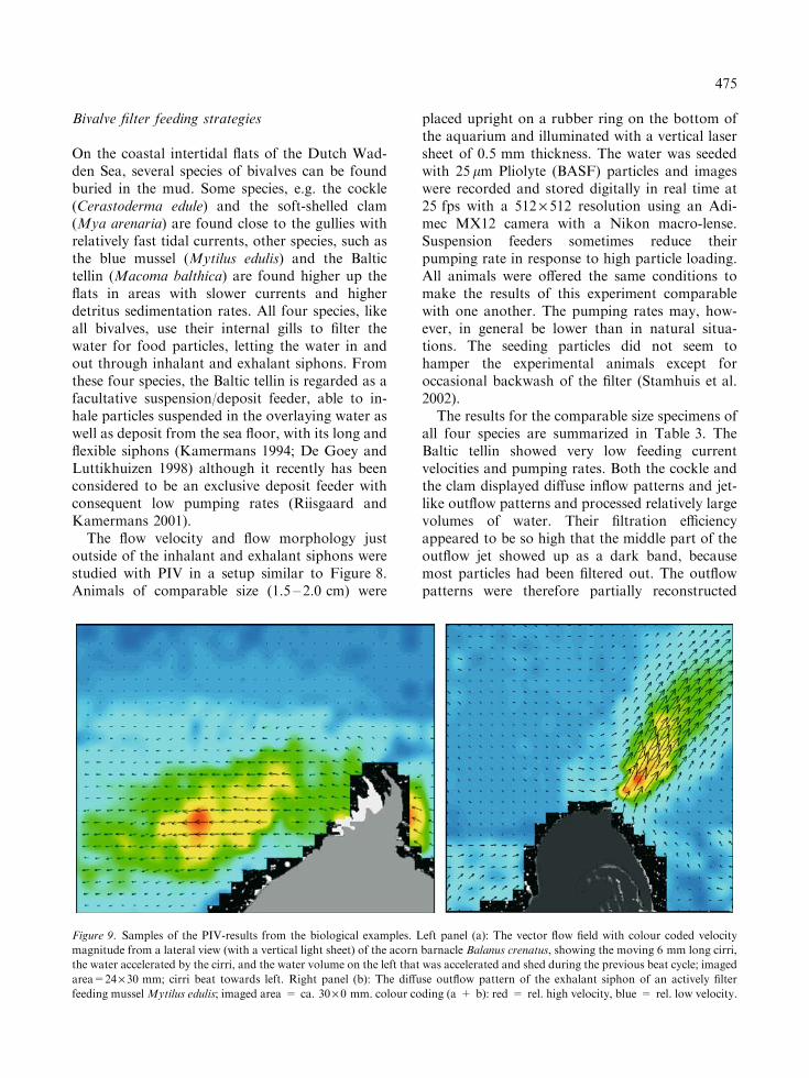
The results from kinematic and PIV analysesshowed that the cirri accelerate fast during the firstpart of the power stroke and that water movesthrough the cirri at that time at a cirral Reynoldsnumber of about 3 (based on cirrus diameter).During the 2nd half of the power stroke, the watercatches up with the cirri, the Reynolds numberdrops to 0.3, and the cirral filter starts to functionas a paddle. During the recovery stroke, the cirriare folded back towards the test opening and rub-bed along the mouthparts to collect and ingest re-tained particles, and then the cirri flick back to theinitial starting position without much interferencewith the water. Figure 9a shows the flow pattern ofan active barnacle in side view halfway the powerstroke (to the left in the figure). The volume ofwater accelerated and filtered during the previousbeat cycle is still visible as a big yellow–red blob inthe left part of the image. The results indicate thatthe barnacle actively filters the water for foodparticles during the first half of the power stroke.Because the cirral function changes from a filter toa paddle approximately halfway the power stroke,the amount of water that has just been filtered isswept away from the barnacle, probably to makesure that it does not filter the same water again.This seems to guarantee a good and continuousfood supply to the animal.

Figure 8. PIV setup for mapping the flow patterns produced by the beating 6 mm long cirri of the acorn barnacle Balanus crenatus.

The picture in the upper-right corner shows the horizontal and vertical planes that have been illuminated and analysed.

474

Bivalve filter feeding strategies

On the coastal intertidal flats of the Dutch Wad-den Sea, several species of bivalves can be foundburied in the mud. Some species, e.g. the cockle(Cerastoderma edule) and the soft-shelled clam(Mya arenaria) are found close to the gullies withrelatively fast tidal currents, other species, such asthe blue mussel (Mytilus edulis) and the Baltictellin (Macoma balthica) are found higher up theflats in areas with slower currents and higherdetritus sedimentation rates. All four species, likeall bivalves, use their internal gills to filter thewater for food particles, letting the water in andout through inhalant and exhalant siphons. Fromthese four species, the Baltic tellin is regarded as afacultative suspension/deposit feeder, able to in-hale particles suspended in the overlaying water aswell as deposit from the sea floor, with its long andflexible siphons (Kamermans 1994; De Goey andLuttikhuizen 1998) although it recently has beenconsidered to be an exclusive deposit feeder withconsequent low pumping rates (Riisgaard andKamermans 2001).

The flow velocity and flow morphology justoutside of the inhalant and exhalant siphons werestudied with PIV in a setup similar to Figure 8.Animals of comparable size (1.5 – 2.0 cm) were

placed upright on a rubber ring on the bottom ofthe aquarium and illuminated with a vertical lasersheet of 0.5 mm thickness. The water was seededwith 25 lm Pliolyte (BASF) particles and imageswere recorded and stored digitally in real time at25 fps with a 512 · 512 resolution using an Adi-mec MX12 camera with a Nikon macro-lense.Suspension feeders sometimes reduce theirpumping rate in response to high particle loading.All animals were offered the same conditions tomake the results of this experiment comparablewith one another. The pumping rates may, how-ever, in general be lower than in natural situa-tions. The seeding particles did not seem tohamper the experimental animals except foroccasional backwash of the filter (Stamhuis et al.2002).

The results for the comparable size specimens ofall four species are summarized in Table 3. TheBaltic tellin showed very low feeding currentvelocities and pumping rates. Both the cockle andthe clam displayed diffuse inflow patterns and jet-like outflow patterns and processed relatively largevolumes of water. Their filtration efficiencyappeared to be so high that the middle part of theoutflow jet showed up as a dark band, becausemost particles had been filtered out. The outflowpatterns were therefore partially reconstructed

Figure 9. Samples of the PIV-results from the biological examples. Left panel (a): The vector flow field with colour coded velocity

magnitude from a lateral view (with a vertical light sheet) of the acorn barnacle Balanus crenatus, showing the moving 6 mm long cirri,

the water accelerated by the cirri, and the water volume on the left that was accelerated and shed during the previous beat cycle; imaged

area=24· 30 mm; cirri beat towards left. Right panel (b): The diffuse outflow pattern of the exhalant siphon of an actively filter

feeding musselMytilus edulis; imaged area = ca. 30· 0 mm. colour coding (a + b): red = rel. high velocity, blue = rel. low velocity.

475

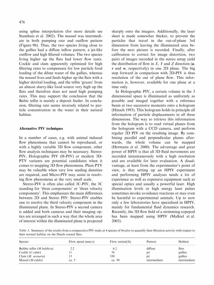
using spline interpolation (for more details seeStamhuis et al. 2002). The mussel was intermedi-ate in both pumping rate and outflow pattern(Figure 9b). Thus, the two species living close tothe gullies had a diffuse inflow pattern, a jet-likeoutflow and high filtered volumes. The two speciesliving higher up the flats had lower flow rates.Cockle and clam apparently optimized for highfiltering rates to compensate for low particle foodloading of the dilute water of the gullies, whereasthe mussel lives and feeds higher up the flats with ahigher detrital loading, and the tellin ‘grazes’ froman almost slurry-like food source very high up theflats and therefore does not need high pumpingrates. This may support the conclusion that theBaltic tellin is mainly a deposit feeder. In conclu-sion, filtering rate seems inversely related to par-ticle concentration in the water in their naturalhabitat.

Alternative PIV techniques

In a number of cases, e.g. with animal inducedflow phenomena that cannot be reproduced, orwith a highly variable 3D flow component, otherflow analysis techniques may be necessary. Stereo-PIV, Holographic PIV (H-PIV) or modern 3D-PTV variants are potential candidates when itcomes to mapping 3D flow phenomena. Plain PTVmay be valuable when very low seeding densitiesare required, and Micro-PIV may assist in resolv-ing flow phenomena at the very small scale.

Stereo-PIV is often also called 3C-PIV, the 3Cstanding for ‘three components’ or ‘three velocitycomponents’. This emphasizes the main differencesbetween 2D and Stereo PIV: Stereo-PIV enablesone to resolve the third velocity component in theilluminated plane. In Stereo-PIV a second camerais added and both cameras and their imaging op-tics are arranged in such a way that the whole areaof interest within the illuminated plane is projected

sharply onto the imagers. Additionally, the lasersheet is made somewhat thicker, to prevent theparticles that travel in the out-of-plane 3rddimension from leaving the illuminated area be-fore the next picture is recorded. Finally, aftercalibration to correct for image distortion, twopairs of images recorded in the stereo setup yieldthe distribution of flow in X, Y and Z direction (u,v and w, respectively) in one 2D plane. The bigstep forward in comparison with 2D-PIV is thusresolution of the out of plane flow. This infor-mation is, however, available for one plane at atime only.

In Holographic PIV, a certain volume in the 3dimensional space is illuminated as uniformly aspossible and imaged together with a referencebeam at two successive moments onto a hologram(Hinsch 1993). This hologram holds in principle allinformation of particle displacements in all threedimensions. The way to retrieve this informationfrom the hologram is to read virtual planes fromthe hologram with a CCD camera, and performregular 2D PIV on the resulting image. By com-bining parallel and perpendicular planes after-wards, the whole volume can be mapped(Hermann et al. 2000). The advantage and greatpower of HPIV is that all 3D fluid movements arerecorded instantaneously with a high resolutionand are available for later evaluation. A disad-vantage, at least from the experimenter’s point ofview, is that setting up an HPIV experimentand performing HPIV analyses needs a lot ofexperience as well as expensive equipment such asspecial optics and usually a powerful laser. Highillumination levels or high energy laser pulsessometimes invoke avoidance reactions or may evenbe harmful to experimental animals. Up to nowonly a few laboratories have specialised in HPIV,mainly for fundamental fluid dynamics research.Recently, the 3D flow field of a swimming copepodhas been mapped using HPIV (Malkiel et al.2003).

Table 3. Summary of the results from a comparative PIV study at 4 species of bivalve to quantify their filtration activity with respect to

their normal habitat on the Dutch coastal flats.

Species Flow speed (mm/s) Flow rate(ml/h) Pattern Habitat

Balthic tellin (M.balthica) 2.2 6.2 diffuse flats

Cockle (C.edule) 11 76 jet gullies

Clam (M. arenaria) 13 330 jet gullies

Mussel (M.edulis) ca. 5 ca. 50 intermediate intermediate

476

Three-dimensional particle tracking velocimetry(3D-PTV) is a technique that has already beenused for quite some time and has also been appliedto complex biological flows (e.g. Spedding 1986).In early 3D-PTV studies, the experimenter had tomanually trace particles in e.g. 2 stereo imagesfrom the same scene, allowing only low seedingdensities and involving labourious analysis. Theresulting 3D vector diagrams showed a resolutionhigh enough to get a good impression of the flowphenomena and local flow velocities, but too lowto derive additional descriptive and analyticalparameters. In the recently developed 3DPTVtechniques, often more than 2 views from the samescene are taken, the seeding density of the fluid hasbeen increased to get higher spatial resolutions andthe analysis has been automated. Three views fromthe same scene yield 3 sets of stereo images insteadof 1 set, and, when placing the cameras in a fixedframe of reference, triple triangulation can beperformed to locate each particle with a highaccuracy . Newly developed image analysis algo-rithms, which are mainly based on statistical pro-cedures and forecasting (Cowen and Monismith1997; Van der Plas and Bastiaans 1998), maymanage to track 1500 particles or more in onevolume. The resulting vector diagrams show areasonable to good spatial resolution, high enoughfor derivation of e.g. vorticity. 3D-PTV may see arevival with these new recording and analysismethods, and the technique seems to be verysuitable for biogenic flows, providing that therecording system has the proper speed and reso-lution.

When the seeding density is not high enough forautomated (3D-) PTV or PIV analysis due tolimitations on the animals side, one can revert toplain PTV as it has already been used for decades(e.g. Strathman 1973; Joergensen 1975; Sponaugle1991; Larsen and Riisgard 2002). Here, the parti-cles are usually located visually and manually, andthe result is a flow field with irregular spacedvectors at a relatively low density. The velocityvectors may be very informative, but the lowvector density makes it difficult to derive gradientparameters (shear, vorticity) without a morecomplex mathematical procedure. The accuracydepends highly on the analysis procedure used,which may range from ‘drawing on a foil on themonitor screen’ to ‘centroiding or peak curve fit-ting at particle images in HR digital pictures’.

At the very small scale (ca. 1 mm), the limitedfocal depth of the camera- microscope-combina-tion may be used to define the plane of interest inPTV or PIV studies (e.g. Klank et al. 2001). Such asystem is usually classified as a Micro-PIV system.However, a very thin lightsheet (e.g. 0.1 mmthickness) may still help to prevent blurred particleimages just above or below the plane of interest(e.g. Van Duren et al. 1998), that increase thenoise and thereby lower the accuracy. Micro-PIV(or PTV) may undergo some improvements inoptical as well as analytical aspects which increasethe accuracy and make this technique moreapplicable for biological micro-applications.

One of the latest developments in pursuit ofhigher resolutions and higher accuracy in PIVanalyses is called Super Resolution PIV (SR-PIV).In SR-PIV, two routes have been followed toachieve higher resolution: a PIV route and a PTVroute. The PIV route can be summarized as firstperforming normal PIV analysis with a normalinterrogation window size, and subsequently takingsmaller and smaller segments of the interrogationwindow using the displacement information fromformer steps, to increase accuracy and resolution,almost down to the single particle image size (Hart1999). The other route combines PTV algorithms,sometimes similar to those used in the latest3D-PTV methods, with classic PIV. A PIV stepprovides a first estimation of the flow velocity,followed by PTV which provides information ongradients within the interrogation area using thevelocity information from the PIV step to improveparticle pairing probabilities (Keane et al. 1995;Cowen andMonismith 1997; Bastiaans et al. 2002).Both routes yield comparable results, the vectordensity may increase more than 10-fold, but thePIV route with recursive correlation seems capableof even more spectacular increases (Hart 1999).

Conclusion

Two-dimensional digital particle image velocime-try appears to be a very useful and versatile tech-nique that can be applied to biogenic orbiologically relevant flows relatively easily. Evenirreproducible and very fast flow events can betackled, when using the right illumination andrecording techniques. Application depends ontolerance to the relatively high level of (laser)

477

illumination, and to the presence of densely seededparticles in the flow, that may hamper the organ-ism or prevent it from behaving naturally. PIVflow analysis can deliver 2D vector flow fields in aninstant, and a number of derivable parametersassist in understanding and describing the flowphenomena studied in a qualitative as well as aquantitative way. Interpretation of the 3D flowpatterns from the 2D PIV cross sections is, how-ever, not trivial and has to be done with care.When doing so, 2D DPIV can greatly assist inunderstanding how an organism interacts with afluid and what it actually does with that fluid, ore.g. how it manages to stand up to externalcurrents.

Acknowledgements

Jan Drent assisted in recording of the bivalve flowfields, Michiel Vos recorded the barnacle flowfields, Sandra Nauwelaerts recorded the vortexring flow fields (cooperation with the University ofAntwerp), Luca van Duren and Per Jonson areacknowledged for the invitation to the BIO-FLOW-2002 symposium. The comments of DrH.U. Riisgaard and 2 anonymous refereesenhanced the paper greatly.

References

Adrian R.J. 1991. Particle imaging techniques for experimental

fluid mechanics. Ann. Rev. Fluid Mech. 23: 261 – 304.

Anderson J.D. 2000. Introduction to Flight (4th int. ed.).

McGraw-Hill, Boston.

Bastiaans R.J.M., der Plas G.A.J. and Kieft R.N. 2002. The

performance of a new PTV algorithm in super-resolution

PIV. Exp. In Fluids 32: 346 – 356.

Cowen E.A. and Monismith S.G. 1997. A hybrid digital particle

tracking velocimetry technique. Exp. In Fluids 22: 199 – 211.

Drucker E.G. and Lauder G.V. 1999. Locomotor forces on a

swimming fish: three-dimensional wake dynamics quantified

using digital particle image velocimetry. J. Exp. Biol. 202:

2393 – 2412.

Goey P. de and Luttikhuizen P. 1998. Deep-burying reduces

growth in intertidal bivalves: field and mesocosm experiments

with Macoma balthica. J. Exp. Mar. Biol. Ecol. 228: 327 –

337.

Hart D.P. 1999. Super-resolution PIV by recursive local-

correlation. J. Visualisation 10: 1 – 10.

Hermann S., Hinrichs H., Hinsch K. and Surmann C. 2000.

Coherence concepts in holographic particle image velocime-

try. Exp. In Fluids 29(Suppl.): S108 – S116.

Hinsch K.D. 1993. Particle image velocimetry. In: Sirohi R.S.

(ed.), Speckle Metrology. Marcel Dekker Inc, New York, pp.

235 – 342.

Joergensen C.B. 1975. On gill function in the mussel Mytilus

edulis L. Ophelia 13: 187 – 232.

Jones J.D.C. (ed.), 1997. Particle image velocimetry. Meas. Sci.

Technol. 8(12): 1379–1583.

Kamermans P. 1994. Similarity in food source and timing of

feeding in deposit- and suspension-feeding bivalves. Mar.

Ecol. Prog. Ser. 104: 63 – 75.

Keane R.D. and Adrian R.J. 1992. Theory of cross-correlation

analysis of PIV images. Appl. Sci. Res. 49: 191 – 215.

Keane R.D., Adrian R.J. and Zhang Y. 1995. Super-resolu-

tion particle image velocimetry. Meas. Sci. Technol. 6:

754 – 768.

Klank H.G., Goranovic G., Kutter J.P., Gjelstrup H., Mi-

chelsen J. and Westergaard C.H. 2001. Micro PIV measure-

ments in micro cell sorters and mixing structures with three

dimensional flow behavior. CD-ROM proceedings 4th Int.

Symp. on PIV, Gottingen, Paper, Paper 1161, pp. 1 – 12

Larsen P.S. and Riisgard H.U. 2002. On ciliary sieving in

pumping bryozoans. J. Sea Res. 48: 181 – 195.

Lighthill J. 1986. An Informal Introduction to Theoretical

Fluid Mechanics. Oxford University Press, Oxford.

Malkiel E., Sheng J., Katz J. and Strickler J.R. 2003. The three-

dimensional flow field generated by a feeding calanoid

copepod measured using digital holography. J. Exp. Biol.

206: 3657 – 3666.

Muller U.K., den Heuvel B.L.E., Stamhuis E.J. and Videler J.J.

1997. Fish foot 23 prints: morphology and energetics of the

wake behind a continuously swimming mullet (Chelon lab-

rosus- Risso). J. Exp. Biol. 200: 2893 – 2906.

Raffel M., Willert C. and Kompenhans J. 1998. Particle Image

Velocimetry, A Practical Guide. Springer-Verlag, Berlin.

Riisgaard H.U. and Kamermans P. 2001. Switching between

deposit and suspension feeding in coastal zoobenthos. In:

Reise K. (ed.), Ecological Comparisons of Sedimentary

Shores. Ecological Studies Vol. 151. Springer Verlag, Berlin,

pp. 73 – 101.

Spedding G.R. 1986. wake of a Jackdaw (Corvus monedula) in

slow flight. J. Exp. Biol. 125: 287 – 307.

Spedding G.R. and Rignot E.J.M. 1993. Performance analysis

and application of grid interpolation techniques for fluid

flows. Exp. In Fluids 15: 417 – 430.

Spedding G.R., Hedenstrom A. and Rosen M. 2003. Quanti-

tative studies of the wakes of freely flying birds in a low-

turbulence wind tunnel. Exp. In Fluids (in press).

Sponaugle S. 1991. Flow patterns and velocities around a sus-

pension-feeding gorgonian polyp: evidence from physical

models. J. Exp. Mar. Biol. Ecol. 148: 135 – 145.

Stamhuis E.J. and Videler J.J. 1995. Quantitative flow analysis

around aquatic animals using laser sheet particle image

velocimetry. J. Exp. Biol. 198: 283 – 294.

Stamhuis E.J., Videler J.J., Van Duren L.A. and Muller U.K.

2002. Applying digital particle image velocimetry to animal-

generated flows: Traps, hurdles and cures in mapping steady

and unsteady flows in Re regimes between 10�2 and 105. Exp.

In Fluids 33: 801 – 813.

Stanislas M., Kompenhans J. and Westerweel J. (eds) 2000.

Particle Image Velocimetry, Progress Towards Industrial

Application. Kluwer Academic Publishers, London.

478

Strathmann R. 1973. Function of lateral cilia in suspension

feeding of lophophorates (Brachiopoda, Phoronida, Ectopr-

octa). Mar. Biol. 23: 129 – 136.

der Plas G.J. and Bastiaans R.J.M. 1998. Accuracy and reso-

lution of a fast PTV- algorithm suitable for HiRes-PV. In:

Grant I. and Carlomagno G.M. (eds), Proceedings of the 8th

International Symposium on Flow Visualisation. Sorrento,

Italy, pp. 1/1 – 1/12.

Van Duren L.A., Stamhuis E.J. and Videler J.J. 1998. Reading

the copepods personal ads: increasing encounter probability

with hydromechanical signals. Phil. Trans. R. Soc. Lond. B

353: 691 – 700.

Vogel S. and LaBarbera M. 1978. Simple flow tanks for

research and teaching. Bioscience 28: 638 – 643.

Vogel S. 1994. Life in Moving Fluids, the Physical Biology of

Flow (2nd ed.). Princeton Press, New Jersey.

Vollmers H., Kreplin H.-P. and Meier H.U. 1983. Separation

and vortical-type flow around a prolate spheroid – evaluation

of relevant parameters. NATO-AGARD Conference Pro-

ceedings No. 342, pp. 14/1 – 14/14.

Vollmers H. 2001. Detection of vortices and quantitative eval-

uation of their main parameters from experimental velocity

data. Meas. Sci. Technol. 12: 1199 – 1207.

Westerweel J. 1993. Digital Particle Image Velocimetry – The-

ory and Application. Delft University Press, Delft.

Westerweel J. 1997. Fundamentals of digital PIV. Meas. Sci.

Technol. 8(12): 1379 – 1392.

Westerweel J., Dabiri D. and Gharib M. 1997. The effect of a

discrete window offset on the accuracy of cross-correlation

analysis of PIV recordings. Exp. In Fluids 23: 20 – 28.

Willert C.E. and Gharib M. 1991. Digital particle image ve-

locimetry. Exp. In Fluids 10: 181 – 193.

Zirbel M.J., Veron F. and Latz M.I. 2000. The reversible effect

of flow on the morphology of Ceratocorys horrida (Peridini-

ales, Dinophyta). J. Phycol. 36: 46 – 58.

479