Basic Regression Analysis with Time Series Data · Basic Regression Analysis with ... the current...

© 2013 Cengage Learning. All Rights Reserved. May not be scanned, copied or duplicated, or posted to a publicly accessible website, in whole or in part.

Chapter 10

Basic Regression Analysis with Time Series Data

Wooldridge: Introductory Econometrics: A Modern Approach, 5e


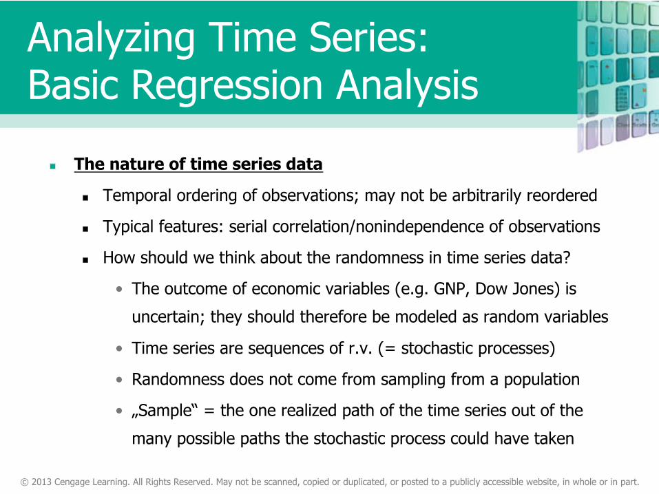
The nature of time series data

Temporal ordering of observations; may not be arbitrarily reordered

Typical features: serial correlation/nonindependence of observations

How should we think about the randomness in time series data?

•  The outcome of economic variables (e.g. GNP, Dow Jones) is

uncertain; they should therefore be modeled as random variables

•  Time series are sequences of r.v. (= stochastic processes)

•  Randomness does not come from sampling from a population

•  „Sample“ = the one realized path of the time series out of the

many possible paths the stochastic process could have taken

Analyzing Time Series: Basic Regression Analysis


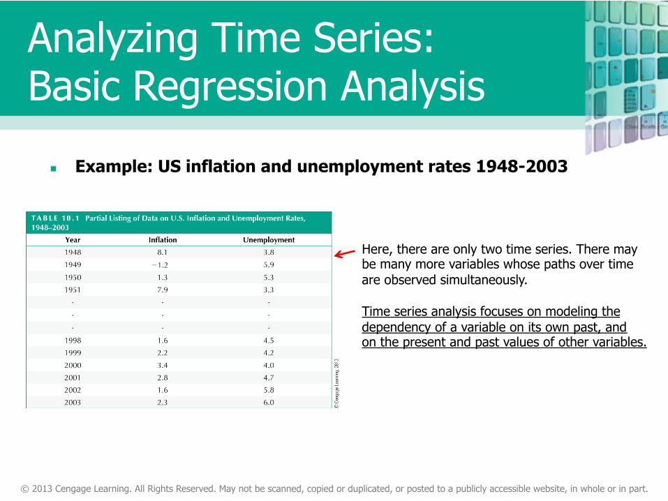
Example: US inflation and unemployment rates 1948-2003

Here, there are only two time series. There may be many more variables whose paths over time are observed simultaneously. Time series analysis focuses on modeling the dependency of a variable on its own past, and on the present and past values of other variables.



Examples of time series regression models

Static models

In static time series models, the current value of one variable is

modeled as the result of the current values of explanatory variables

Examples for static models There is a contemporaneous relationship between unemployment and inflation (= Phillips-Curve).

The current murderrate is determined by the current conviction rate, unemployment rate, and fraction of young males in the population.



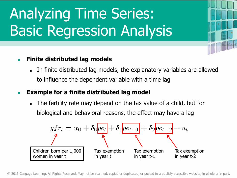
Finite distributed lag models

In finite distributed lag models, the explanatory variables are allowed

to influence the dependent variable with a time lag

Example for a finite distributed lag model

The fertility rate may depend on the tax value of a child, but for

biological and behavioral reasons, the effect may have a lag

Children born per 1,000 women in year t

Tax exemption in year t

Tax exemption in year t-1

Tax exemption in year t-2



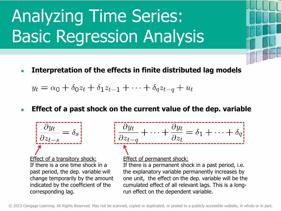
Interpretation of the effects in finite distributed lag models

Effect of a past shock on the current value of the dep. variable

Effect of a transitory shock: If there is a one time shock in a past period, the dep. variable will change temporarily by the amount indicated by the coefficient of the corresponding lag.

Effect of permanent shock: If there is a permanent shock in a past period, i.e. the explanatory variable permanently increases by one unit, the effect on the dep. variable will be the cumulated effect of all relevant lags. This is a long-run effect on the dependent variable.



Graphical illustration of lagged effects

For example, the effect is biggest after a lag of one period. After that, the effect vanishes (if the initial shock was transitory). The long run effect of a permanent shock is the cumulated effect of all relevant lagged effects. It does not vanish (if the initial shock is a per-manent one).



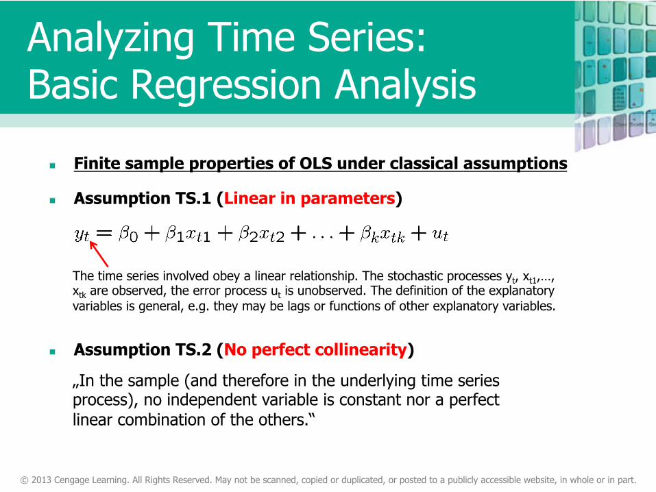
Finite sample properties of OLS under classical assumptions

Assumption TS.1 (Linear in parameters)

Assumption TS.2 (No perfect collinearity)

„In the sample (and therefore in the underlying time series process), no independent variable is constant nor a perfect linear combination of the others.“

The time series involved obey a linear relationship. The stochastic processes yt, xt1,…, xtk are observed, the error process ut is unobserved. The definition of the explanatory variables is general, e.g. they may be lags or functions of other explanatory variables.



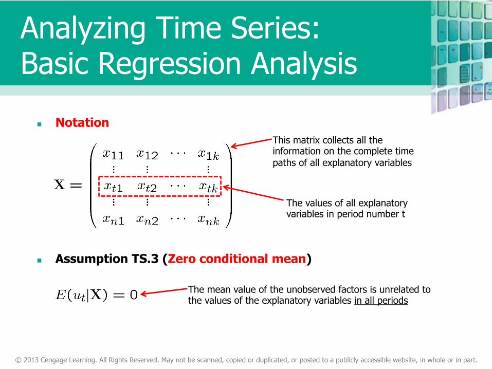
Notation

Assumption TS.3 (Zero conditional mean)

The mean value of the unobserved factors is unrelated to the values of the explanatory variables in all periods

The values of all explanatory variables in period number t

This matrix collects all the information on the complete time paths of all explanatory variables



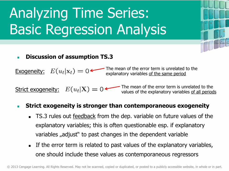
Discussion of assumption TS.3

Strict exogeneity is stronger than contemporaneous exogeneity

TS.3 rules out feedback from the dep. variable on future values of the

explanatory variables; this is often questionable esp. if explanatory

variables „adjust“ to past changes in the dependent variable

If the error term is related to past values of the explanatory variables,

one should include these values as contemporaneous regressors

The mean of the error term is unrelated to the values of the explanatory variables of all periods

The mean of the error term is unrelated to the explanatory variables of the same period Exogeneity:

Strict exogeneity:



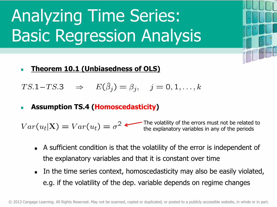
Theorem 10.1 (Unbiasedness of OLS)

Assumption TS.4 (Homoscedasticity)

A sufficient condition is that the volatility of the error is independent of

the explanatory variables and that it is constant over time

In the time series context, homoscedasticity may also be easily violated,

e.g. if the volatility of the dep. variable depends on regime changes

The volatility of the errors must not be related to the explanatory variables in any of the periods



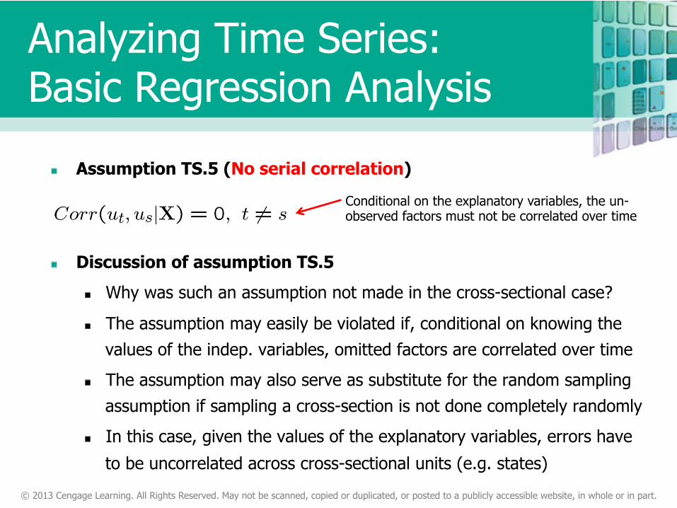
Assumption TS.5 (No serial correlation)

Discussion of assumption TS.5

Why was such an assumption not made in the cross-sectional case?

The assumption may easily be violated if, conditional on knowing the values of the indep. variables, omitted factors are correlated over time

The assumption may also serve as substitute for the random sampling assumption if sampling a cross-section is not done completely randomly

In this case, given the values of the explanatory variables, errors have

to be uncorrelated across cross-sectional units (e.g. states)

Conditional on the explanatory variables, the un-observed factors must not be correlated over time



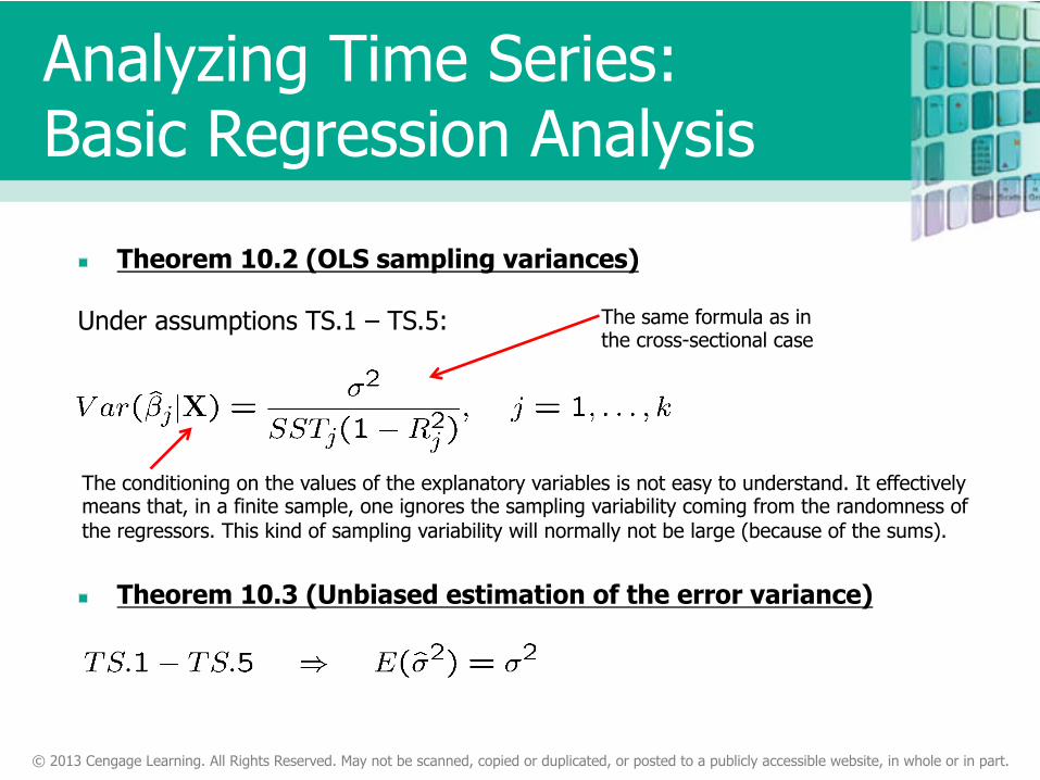
Theorem 10.2 (OLS sampling variances)

Theorem 10.3 (Unbiased estimation of the error variance)

Under assumptions TS.1 – TS.5: The same formula as in the cross-sectional case

The conditioning on the values of the explanatory variables is not easy to understand. It effectively means that, in a finite sample, one ignores the sampling variability coming from the randomness of the regressors. This kind of sampling variability will normally not be large (because of the sums).



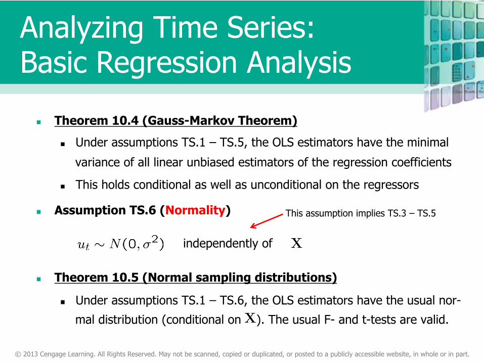
Theorem 10.4 (Gauss-Markov Theorem)

Under assumptions TS.1 – TS.5, the OLS estimators have the minimal

variance of all linear unbiased estimators of the regression coefficients

This holds conditional as well as unconditional on the regressors

Assumption TS.6 (Normality)

Theorem 10.5 (Normal sampling distributions)

Under assumptions TS.1 – TS.6, the OLS estimators have the usual nor-

mal distribution (conditional on ). The usual F- and t-tests are valid.

independently of

This assumption implies TS.3 – TS.5



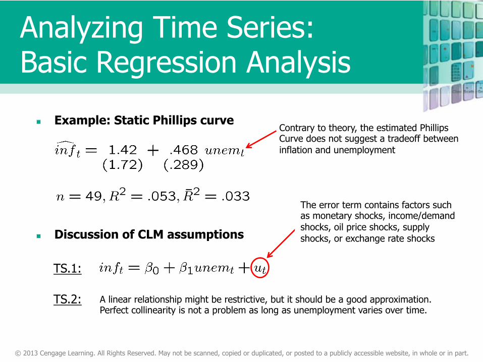
Example: Static Phillips curve

Discussion of CLM assumptions

Contrary to theory, the estimated Phillips Curve does not suggest a tradeoff between inflation and unemployment

A linear relationship might be restrictive, but it should be a good approximation. Perfect collinearity is not a problem as long as unemployment varies over time.

TS.1:

The error term contains factors such as monetary shocks, income/demand shocks, oil price shocks, supply shocks, or exchange rate shocks

TS.2:



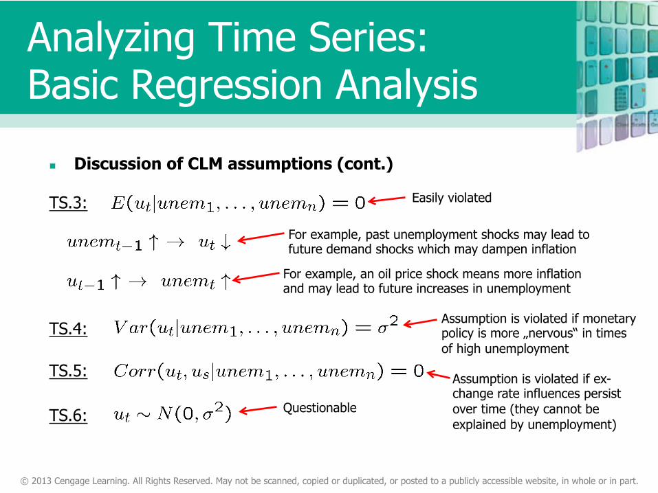
Discussion of CLM assumptions (cont.)

TS.3:

For example, past unemployment shocks may lead to future demand shocks which may dampen inflation

For example, an oil price shock means more inflation and may lead to future increases in unemployment

TS.4:

TS.5:

Assumption is violated if monetary policy is more „nervous“ in times of high unemployment

TS.6:

Assumption is violated if ex-change rate influences persist over time (they cannot be explained by unemployment)

Questionable

Easily violated



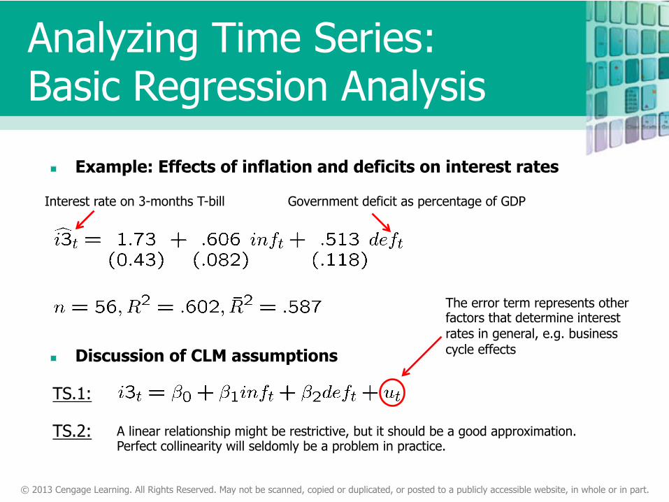
Example: Effects of inflation and deficits on interest rates

Discussion of CLM assumptions

A linear relationship might be restrictive, but it should be a good approximation. Perfect collinearity will seldomly be a problem in practice.

TS.1:

The error term represents other factors that determine interest rates in general, e.g. business cycle effects

TS.2:

Interest rate on 3-months T-bill Government deficit as percentage of GDP



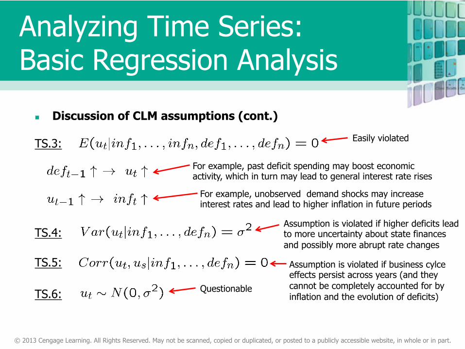
Discussion of CLM assumptions (cont.)

TS.3:

For example, past deficit spending may boost economic activity, which in turn may lead to general interest rate rises

For example, unobserved demand shocks may increase interest rates and lead to higher inflation in future periods

TS.4:

TS.5:

Assumption is violated if higher deficits lead to more uncertainty about state finances and possibly more abrupt rate changes

TS.6:

Assumption is violated if business cylce effects persist across years (and they cannot be completely accounted for by inflation and the evolution of deficits)

Questionable

Easily violated



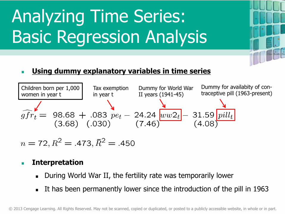
Using dummy explanatory variables in time series

Interpretation

During World War II, the fertility rate was temporarily lower

It has been permanently lower since the introduction of the pill in 1963

Children born per 1,000 women in year t

Tax exemption in year t

Dummy for World War II years (1941-45)

Dummy for availabity of con-traceptive pill (1963-present)



Time series with trends

Example for a time series with a linear upward trend



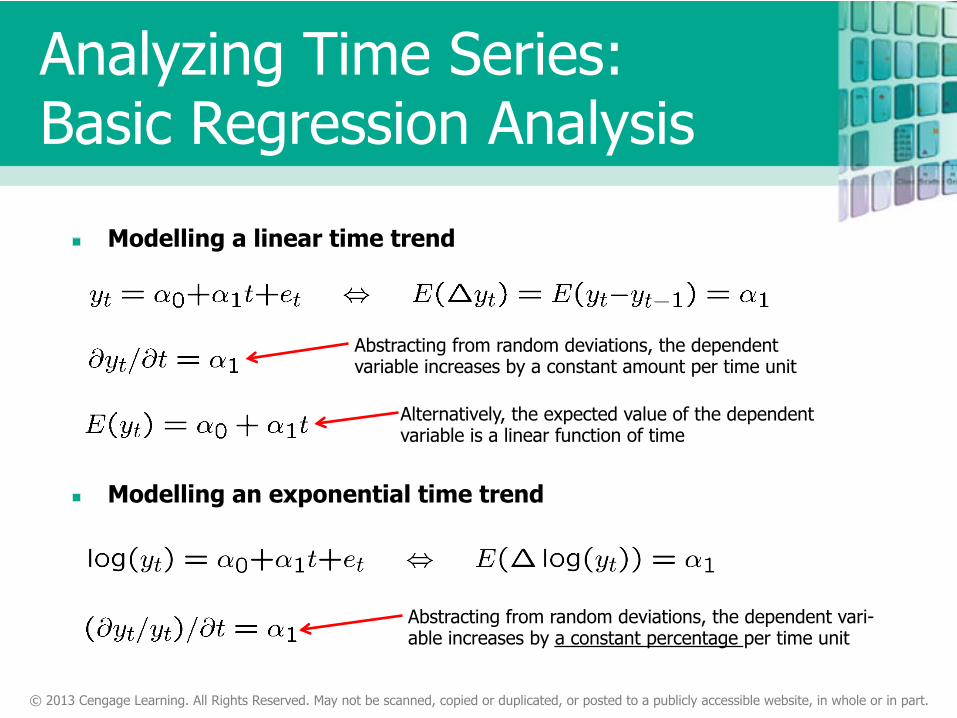
Modelling a linear time trend

Modelling an exponential time trend

Abstracting from random deviations, the dependent variable increases by a constant amount per time unit

Alternatively, the expected value of the dependent variable is a linear function of time

Abstracting from random deviations, the dependent vari-able increases by a constant percentage per time unit



Example for a time series with an exponential trend

Abstracting from random deviations, the time series has a constant growth rate



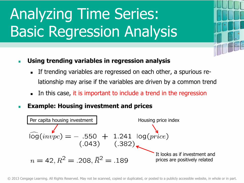
Using trending variables in regression analysis

If trending variables are regressed on each other, a spurious re-

lationship may arise if the variables are driven by a common trend

In this case, it is important to include a trend in the regression

Example: Housing investment and prices

Per capita housing investment Housing price index

It looks as if investment and prices are positively related



Example: Housing investment and prices (cont.)

When should a trend be included?

If the dependent variable displays an obvious trending behaviour

If both the dependent and some independent variables have trends

If only some of the independent variables have trends; their effect on

the dep. var. may only be visible after a trend has been substracted

There is no significant relationship between price and investment anymore



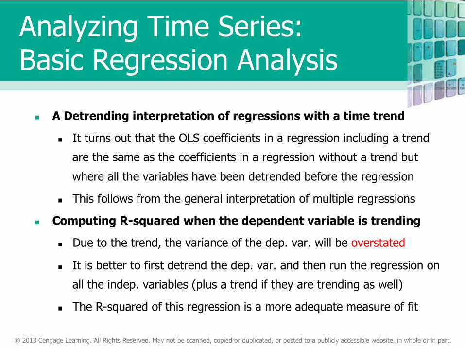
A Detrending interpretation of regressions with a time trend

It turns out that the OLS coefficients in a regression including a trend

are the same as the coefficients in a regression without a trend but

where all the variables have been detrended before the regression

This follows from the general interpretation of multiple regressions

Computing R-squared when the dependent variable is trending

Due to the trend, the variance of the dep. var. will be overstated

It is better to first detrend the dep. var. and then run the regression on

all the indep. variables (plus a trend if they are trending as well)

The R-squared of this regression is a more adequate measure of fit



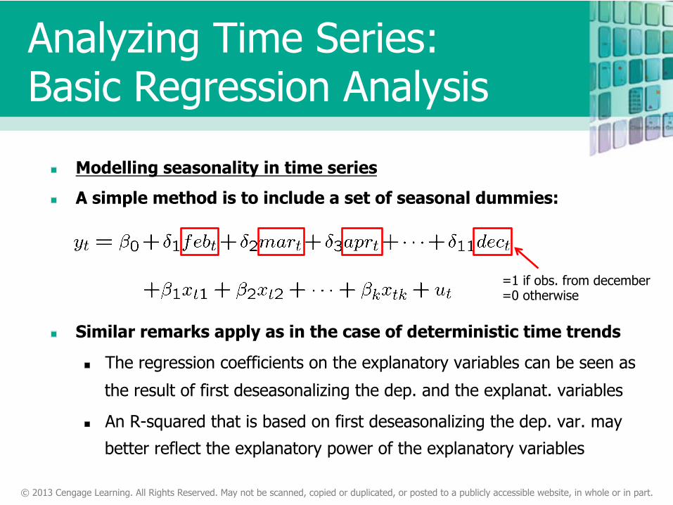
Modelling seasonality in time series

A simple method is to include a set of seasonal dummies:

Similar remarks apply as in the case of deterministic time trends

The regression coefficients on the explanatory variables can be seen as

the result of first deseasonalizing the dep. and the explanat. variables

An R-squared that is based on first deseasonalizing the dep. var. may

better reflect the explanatory power of the explanatory variables

=1 if obs. from december =0 otherwise


Basic Regression Analysis with Time Series Data · Basic Regression Analysis with ... the current...

Documents

Transcript of Basic Regression Analysis with Time Series Data · Basic Regression Analysis with ... the current...