BASIC RADIO PROPAGATION PREDICTIONS

'FOR OCTOBER 1945

THREE MONTHS IN ADVANCE

ISSUED'

JULY 1945

PREPARED BY INTERSERVICE RADIO PROPAGATION LABORATORY

National Bureau of Standards

Washington 25, D. C.

“ Th,is document contains information affecting the national defense of

the United States within the meaning of the Espionage Act, 50 U. S. C.

31 and 32. Its transmission or the revelation of its contents in any manner

to an unauthorized person is prohibited by law.”

IRPL-Dll Issued 1 July 1945

INTERSERVICE RADIO PROPAGATION LABORATORY

NATIONAL BUREAU OF STANDARDS WASHINGTON 25, D. C.

Organized Under Joint U. S. Communications Board

BASIC RADIO PROPAGATION PREDICTIONS FOR OCTOBER 1945

THREE MONTHS IN ADVANCE

The monthly reports of the IRPL-D series are now distributed to the Army as the TB 11-499 series, by the Adjutant General; to the Navy as the DNC-13-1 series, by the Registered Publications Section, Division of Naval Communications; and to others by the IRPL.

This IRPL-D series is a monthly supplement to the IRPL Radio Propagation Handbook, Part 1, issued by the Army as TM 11-499 and by the Navy as DNC-13-1, and is required in order to make practical application of the basic Handbook.

Comments are invited from users of this report as to the accuracy of predictions when applied to the solution of specific radio propagation problems. Such comments or queries concerning radio propagation should be addressed as follows:

For the Army: Headquarters, Army Service Forces, Office of the Chief Signal Officer, Washington 25, D. C. Attention: SPSOL.

For the Navy: Chief of Naval Operations, Navy Department, Washington 25, D. C. (DNC-20-F).

For Others: Interservice Radio Propagation Laboratory, National Bureau of Standards, Washington 25, D. C.

CONTENTS

I. Terminology_ Page 2 II. World-wide prediction charts and their uses- Page 2

World map showing zones covered by prediction charts, and auroral zones.- Fig. 1

E2-zero-muf, in Me, W zone, predicted for October 1945_ Fig. 5

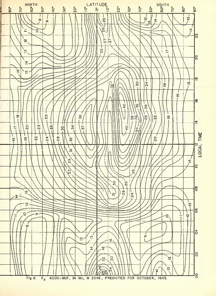
E2-4000-muf, in Me, W zone, predicted for October 1945__ Fig. 6

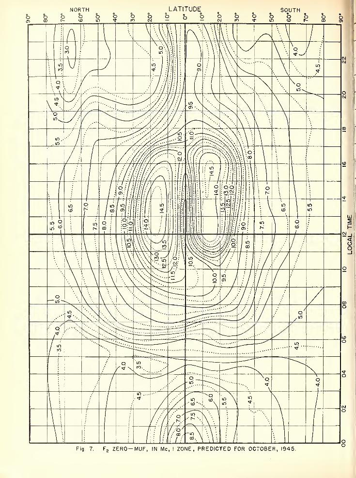
E2-zero-muf, in Me, / zone, predicted for October 1945_ Fig. 7

E2-4000-muf, in Me, I zone, predicted for October 1945_ Fig. 8

E2-zero-muf, in Me, E zone, predicted for October 1945_ - - Fig. 9

E2-4000-muf, in Me, E zone, predicted for October 1945__ Fig. 10

.E-layer 2000-muf, in Me, predicted for October 1945__ _ _ Fig. 11

Median fEs, in Me, predicted for October 1945_ Fig. 12

Percentage of time occurrence for Es in excess of 15 Me, predicted for October 1945__ Fig. 15

III. Determination of great-circle distances, bear¬ ings, location of transmission control points, solar zenith angles_ Page 2

Great-circle chart, centered on equator, with small circles indicating distances in kilometers_ Fig. 2

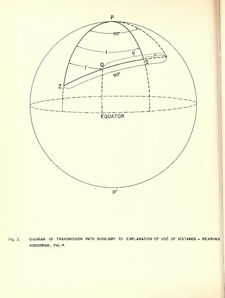
Diagram of transmission path auxiliary to explanation of use of distance- bearing nomogram, figure 4- Fig. 3

III. Determination, etc.—Continued.

Nomogram for obtaining great-circle distances, bearings, latitude and longi¬ tude of transmission control points, solar zenith angles. Conversion scale for various distance units_ Fig. 4

IV. Calculation of maximum usable frequencies aiKpoptimum working frequencies_ Page 3

Nomograms for transforming F2-zero- muf and E2-4000-muf to equivalent maximum usable frequencies at inter¬ mediate transmission distances; con¬ version scale for obtaining optimum working frequencies_ Fig. 13

Nomogram for transforming E-layer 2000-muf to equivalent maximum usable frequencies and optimum work¬ ing frequencies due to combined effect of E layer and El layer at other trans¬ mission distances_ Fig. 14

V. Absorption, distance range, and lowest useful . high frequency_ Page 4

Absorption index chart (excluding au¬ roral absorption) for October. _ _Fig. 16

VI. Sample muf and owf calculations_ Page 5 For short paths (under 4000 km) page 5,

table 1, page 6, and Fig. 17. For long paths (over 4000 km) page 5,

table 2, page 7, and Fig. 18.

650802—45--1 [1]

I. TERMINOLOGY

The following symbols are used, as recom¬ mended by the International Radio Propagation Conference held in Washington, D. C., 17 April to 5 May 1944.

/°/^2 = ordinary-wave critical frequency for the F2 layer. The term night F layer will no longer be used. The term F'2 layer is now used for the night F as well as the daytime F'2 layer.

/'F2 = extraordinary-wave critical fre¬ quency for the F2 layer.

Es — sporadic, or abnormal E.

Note.—The designation FF-

II. WORLD-WIDE PREDICTION

The charts, figures 5 to 11, present world-wide predictions of monthly average maximum usable frequencies for October 1945. Conditions may be markedly different on disturbed days, especially in or near the auroral zones, shown on the map of figure 1. The method of prediction is discussed in the IRPL Radio Propagation Handbook, Part 1, War Dept. TM 11-499, Navy Dept. DNC-13-1, p. 52. 53.

Although ionosphere characteristics are roughly similar for locations of equal latitude, there is also a considerable variation with longitude, espe¬ cially in the case of the F2 layer. This “longitude effect” seems to be related to geomagnetic latitude. Attention was first called to this effect in the report “Radio Propagation Conditions” issued 10 Sept. 1943; it was brought into general operational use in the next issue (14 Oct. 1943).

The longitude effect in the F2 layer is taken care of by providing world charts for three zones, in each of which the ionosphere characteristics are independent of longitude, for practical pur¬ poses. These zones are indicated on the world map, figure 1.

fEs=highest frequency of Es reflec¬ tions.

muf or MUF = maximum usable frequency, owf or OWF = optimum working frequency.

4000-muf chart = contour chart of muf for 4000- kilometer paths.

2000-muf chart = contour chart of muf for 2000- kilometer paths.

Zero-muf chart=contour chart of vertical-inci¬ dence critical frequency, ex¬ traordinary wave.

K = absorption index (ratio of actual absorption to absorption at the subsolar point).

has been replaced by F-.

CHARTS AND THEIR USES

Two F'2 charts are provided for each zone, one of which, the “zero-muf chart,” shows the vertical- incidence muf, or the critical frequency for the extraordinary wave, and the other, the “4000- muf chart,” shows the muf for a transmission dis¬ tance of 4000 km. Do not confuse the zero-muf charts with the f°F2 charts appearing in the pre¬ vious IRPL reports “Radio Propagation Condi¬ tions.” (Values of A2-zero-muf exceed those of f°F2 for the same location and local time by an amount approximately equal to half the gyro- frequency for the location. See IRPL Radio Propagation Handbook, Part 1 (War Dept. TM 11-499 and Navy Dept, DNC-13-1), p. 18, 19, 28, and fig. 9).

The longitude variation is operationally negli¬ gible in the case of the normal E layer and there¬ fore only one A-layer chart is provided.

The variation of fE.s with geomagnetic latitude seems to be well marked and important. Conse¬ quently, the fEs charts are constructed on the basis of geomagnetic latitude. Since there are, as yet, insufficient correlated data, the fEs charts are much less precise than the other charts. Instructions for use of these charts appear in section IV, 3.

III. DETERMINATION OF GREAT-CIRCLE DISTANCES, BEARINGS, LOCATION OF

TRANSMISSION CONTROL POINTS, SOLAR ZENITH ANGLES

1. The first step in any radio propagation cal¬ culation is the determination of the transmission path, which is the great-circle distance between transmitting and receiving stations. Use the world map, figure 1, and the great-circle chart, figure 2, for this purpose, as follows:

a. Place a piece of transparent paper over the map, figure 1, and draw upon it a convenient refer¬ ence latitude line, the locations of the transmit¬ ting and receiving stations, and the meridian whose local times are to be used as the times for calculation.

b. Place this transparency over the chart, figure 2. and, keeping the reference line at the proper

latitude, slide the transparency horizontally until the terminal points marked on it either fall on the same great-circle curve, or fall the same propor¬ tional distance between adjacent great-circle curves. Draw in the path.

c. Locate the midpoint of the path, for paths under 4000 km, or the “control points,” 2000 km from either end of the path, for paths greater than 4000 km, and use for this purpose the small circles of figure 2.

d. Place the transparency over the predicted chart at the proper latitude and local time, and read the values of muf off the chart, as direted in section IV.

[2]

2. Great-circle distances, bearings, location of midpoints, or other “control points” 2000 km in from the ends of the transmission path, as well as solar zenith angles, may he readily obtained from the nomogram, figure 4.

Referring to the auxiliary diagram, figure 3, let Z and S he the locations of transmitting and re¬ ceiving stations, where Z is the west, and S t lie east end of the path. Consider north latitudes-f and south latitudes — , and take the absolute value of any sums or differences of angles (without re¬ gard to sign). Use the nomogram, figure 4, as follows:

a. To obtain the great-circle distances ZS:

(1) Draw slant line from (lat. of Z —hit. of S)

measured up from bottom of left scale, to (lat. of Z + lat. of S), measured down from top of right scale.

(2) From the longitude difference between S and Z, on bottom scale, measured from left to right, draw vertical line to the slant line obtained in (1). (Use either the longitude difference or 360° —the longitude difference, whichever is the smaller.)

(3) From the intersection, draw a horizontal line to the left scale. This gives ZS in degrees.

(4) Convert the distance ZS to kilometers, statute miles, or nautical miles, by using the scale at the bottom of figure 4.

b. To obtain the bearing angle PZS:

(1) Subtract the distance ZS (in degrees) from 90° to get A.

(2) Draw slant line from (lat Z —A), meas¬ ured up from bottom on left scale, to (lat. Z + A), measured down from top on right scale.

(3) From 90° — lat. S) on left, measured up from bottom on left scale, draw horizontal line until it intersects previous slant line.

(4) From the intersection, draw a vertical line to the bottom scale, which gives the bearing angle PZS, in degrees. c. To obtain the bearing angle PSZ:

(1) Repeat steps (1), (2), (3) and (4) in b. interchanging Z and S in all computations. The

result obtained is the interior angle PSZ, in degrees.

(2) The bearing angle PSZ is 360° minus the result obtained in (1) (since bearings are cus¬ tomarily given clockwise from due north).

d. To obtain latitude of Q (mid, or other, point of path) :

(11 Obtain ZQ in degrees. If Q is the mid¬ point of the path, Z^Q will be equal to one-half ZS. If Q is one of the 2000-km “control points,” Z,Q will be approximately 18°, or ZS~ 18°.

(2) Subtract ZQ from 90° to get A'. (3) Draw slant line from (lat. Z —A'), meas¬

ured up from bottom of left scale, to (lat. Z + A'), measured down from top on right scale.

(4) From bearing angle PZS, measured to right on bottom scale, draw vertical line to the above slant line.

(5) From Ibis intersection, draw horizontal line to left scale.

(6) Subtract the reading given from 90° to give latitude of Q in degrees.

e. To obtain longitude difference, t', between Z and Q:

(1) Draw straight line (lat. Z —hit. Q), meas¬ ured up from the bottom on left-hand scale, to (lat. Z + lat. Q), measured down from the top on right- hand scale.

(2) From the left side, at ZQ. in degrees, draw a horizontal line to the above slant line.

(3) From the intersection, drop a vertical line to bottom scale to get t' in degrees.

f. To obtain solar zenith angle, ip, at a given place:

(1) Let the declination of the sun be d, and let Z be the place under consideration.

(2) Draw straight line from (lat. Z~d), meas¬ ured up from bottom on left scale, to (lat. Z + d), measured down on right scale.

(3) From [ (12 —local time of Z, in hours) X15] degrees, on bottom scale, measured from left to right, draw a vertical line to the slant line above.

(4) From this intersection, draw a horizontal line to the left scale. This gives ip, in degrees.

IV. CALCULATION OF MAXIMUM USABLE FREQUENCIES AND OPTIMUM WORKING FREQUENCIES

1. PROCEDURE FOR DETERMINATION OF MUF OR OWF FOR TRANSMISSION

DISTANCES UNDER 4000 KW

Radio propagation over distances up to 4000 km is usually determined by ionospheric conditions at the midpoint of the great-circle path between transmitting and receiving station.

Use the following procedure for obtaining the muf and owf for distances less than 4000 km:

a. Locate the midpoint of the transmission path. (Methods for doing this are given in the preceding section of this report.)

b. Read the values of F2-zero-muf, F2-4000-

muf, and A*-layer 2000-muf for the midpoint of the path at the local time for this midpoint. Be sure to choose the F2 charts for the geographical zone in which the midpoint lies. (For a path just 4000 km long the F2-zero muf need not be read; omit step c below, in this case, since the F2-4000-muf is the /^2-layer path muf.)

c. Place a straightedge between the values of F2-zero-muf and F2-4000-mnf at the left- and right-hand sides, respectively, of the grid nomo-

[3]

gram, figure 13, and read the value of the muf for the actual path length at the intersection point of the straightedge with the appropriate vertical dis¬ tance line. (Note that the 4000-muf scale on the grid nomogram is only for frequencies up to 35 Me. To use the nomogram for higher values of 7^2-4000- muf multiply both the zero-muf and the 4000-muf scales by two, and use as instructed above.)

d. The U2-layer optimum working frequency (owf) is 85 percent of the muf, to allow a margin of safety for day-to-day variations; to determine the owf, use the auxiliary scale at the right of the grid nomogram of figure 13. (For values of muf greater than 35 Me, multiply the muf and owf scales by two.)

e. Place a straightedge between the value of

the ZUlayer 2000-muf located on the left-hand

scale of the nomogram, figure 14, and the value

of the path length on the right-hand scale, and

read the combined E- and /'T-layer muf or owf

for that path length, off the central scale. (The

characteristics of the E layer and of the Fl layer

are sufficiently related that, for most practical

purposes, they may be combined in this manner.)

f. Compare the values of muf or owf obtained

by operations c to e. The higher of the two values thus determined is the muf or owf for the path.

2. PROCEDURE FOR DETERMINATION OF MUF OR OWF FOR TRANSMISSION

DISTANCES GREATER THAN 4000 KM

The complexities of long-distance radio propa¬ gation are such that the simple multihop E or F2 layer calculations do not give accurate results. The following procedure will give results which are operationally satisfactory; the theory involved is outside the scope of this report.

a. Locate the two “control points” 2000 km from the ends of the great-circle distance between transmitting and receiving stations. For very long paths both the “short route” (minor arc of the great-circle path) and the “long route” (major arc) need to be considered.

b. Read the value of the F2-4000-muf, at the local time for each point, at these points, being sure to choose the appropriate zone for each point.

c. Calculate the 7^2-4000-owf for each point (85 percent of the muf) by means of the auxiliary muf-owf scale of figure 13. (For values of muf greater than 35 Me, multiply the muf and owf scales by two.)

d. Compare these two muf or owf values. The lower of the two is the muf or owf for the transmission path under consideration.

e. When one of the control points lies in a region where the /?-2000-muf is greater than the F2- 4000-muf, read the /C-2000-muf at an TT-layer control point 1000 km from the end of the path, instead of the F2-4000-muf, as in step b. Use the /?-2000-muf in step d. instead of the F2-4000- muf or owf.

3. PROCEDURE FOR DETERMINATION OF Es TRANSMISSION

(Note Change in Charts and Procedure)

Sporadic-/? {Es) propagation plays an import¬ ant part in transmission over paths in some parts of the world and at certain times. It may often allow regular transmission at times when regular /^2-layer propagation woidd not. Es data are not yet sufficient to permit accurate calculations of such propagation, but the fEs charts of figures 12 and 15 are given as a guide to Es occurrence.

Since the fEs charts are constructed from con¬ siderations of geomagnetic latitude, three latitude scales are provided at the right of the charts of figures 12 and 15, one for each of the three zones of figure 1 (IF, /, and E).

Until improvements are made the following procedure should be used to find the prevalence of Es propagation over a transmission path,

a. For paths over 4000 km long:

(1) Place the great-circle path transparency prepared in section III. 1. over the median fEs chart, figure 12, using the latitude scale for the zone containing the control point.

(2) Scale fEs at each ZT-layer control point (1000 km from either end of the path), multiply by 5 and subtract 4 Me. The result is the Ws-owf.

(3) Plot as the owf for each control point the highest of the three values; the F2-4000-owf. the /?-2000-owf, and the Es-owf.

b. For paths less than 4000 km long, scale the fEs at the midpoint of the path, using the latitude scale for the appropriate zone, multiply by 5 and subtract 4 Me, and use the resultant frequency as outlined above tor the ZUlayer 2000- muf in the nomogram of figure 14. The result is the Es-owf.

[4]

V. ABSORPTION, DISTANCE RANGE, AND LOWEST USEFUL HIGH FREQUENCY The determination of absorption, distance range,

and lowest useful high frequency is discussed at

length in IRPL Radio Propagation Handbook,

Part 1, p. 69-97 (War Dept. TM 11-499, Navy

Dept. DNC-13-1), and formulas, graphs, and

nomograms for calculation are given there. For

convenience in estimating absorption (exclusive of auroral absorption) over a path, the absorption index (or K) chart, figure 16, is presented. By

superposing on this chart the transparency with the great-circle path, prepared as in section III, 1, the relation of the path to the sun’s zenith angle is readily seen (the sunrise-sunset line corresponds to an absorption index approximately = 0.14).

The absorption is erratic and considerably greater in and near the auroral zones, shown on the map of figure 1; paths passing through or near these zones are subject at times to severe dis¬ turbances.

VI. SAMPLE MUF AND OWF CALCULATIONS 1. FOR SHORT PATHS

Required: The muf and owf for transmission between Washington, D. C. (39.0° N, 77.5° W) and Miami, Fla. (25.7° N, 80.5° AV) for average conditions during the month of October 1945.

Solution:

Let the local time used for this problem be GCT (Z time or that of 0° longitude).

The midpoint of the path is at approximately 32.5° N, 79.0° W. and the transmission path length is approximately 1500 km.

The values of E- and F2-layer muf and owf, and also Es-oyvi for alternate hours, GCT, as deter¬ mined by using the procedure given in section IV, are given in table 1. The final values are pre¬ sented graphically in figure 17. In obtaining the combined muf for all layers, the As-owf is used because of the great variability of the muf.

Figure 17 shows that skip will occur, on the average, during the night hours, if a frequency as high as 8.0 Me is used. A frequency as high as

6.5 Me will not skip, on the average, at any time of day, but its use is not advisable because of (a) the day-to-day variability, causing some proba¬ bility of skip during the night hours, and (b) ionospheric absorption during the daytime, which is more pronounced at low frequencies.

A satisfactory frequency plan to insure continu¬ ous transmission at all times, over a path like this, involves the use of two frequencies, one for night and one for day. Figure 17 shows that a night frequency of 5.6 Me, to be used from 2315 to 1230 GCT, and a day frequency of 11.0 Me, to be used from 1230 to 2315 GCT, would be satisfactory. The periods of usefulness of these frequencies are shown by the heavy dashed line on figure 17.

Periods of time during which transmission is controlled by either the E layer or the F'i layer may be easily recognized by noting the relative proximity of the muf and owf curves of figure 17. Coincidence of the curves indicates control by sporadic-A reflections.

2. FOR LONG PATHS

Required: The muf and owf for transmission between Nagasaki, Japan (33° N, 130° E), and San Francisco, Calif. (37.5° N, 122.4° W), for average conditions during the month of October 1945.

Solution:

Let the local time for this problem be GCT (Z time or that of 0° longitude).

The path length is approximately 9100 km, and the two AV-layer control points A and B, respec¬ tively, are at approximately 46° N, 146° W, and 43° N, 149° E. These are respectively in the I zone and E zone as shown on the map, figure 1. The two AMayer and AVcontrol points, A' and B', respec¬ tively, are located at approximately 44° N, 133° W, and 38° N, 138° E. The bearing of San Fran¬ cisco from Nagasaki is approximately 52°, and of Nag asaki from San Francisco, approximately 305°, both determined bv means of the nomogram of figure 4.

The values of muf and owf over this transmis¬ sion path, as determined by using the procedure of section IV, are given in table 2 for alternate hours, GCT. The final values are shown graphically in figure 18.

Figure 18 shows that skip will occur, on the

average, during the night hours if a frequency as high as 10.0 Me is used, although higher frequencies may be used during a limited portion of the clay.

A good practical arrangement to insure con¬ tinuous transmission at all times is to select three frequencies, in a manner similar to that suggested in the preceding problem. A frequency of 7.5 Me may be used from 0530 to 2015 GCT, a frequency of 18.5 Me may be used from 2120 to 0320 GCT, and a transition frequency of 11.5 Me may be used from 0320 to 0530, and from 2015 to 2120 GCT.

Relative proximity of the muf owf curves of figure 18 indicates that neither Es nor regular E layer controls transmission at any time.

By inspection of the absorption chart, figure 16, and the noise map (fig. 119 of the IRFL Radio Propagation Handbook, Part 1, War Dept. TM 11-499, Navy Dept. DNC-13-1), it may be seen that considerations of the lowest useful high fre¬ quency over this path may be considerable im¬ portance in selecting frequencies for use. Conse¬ quently, in cases of transmission failure on the fre¬ quencies here recommended, particularly in the case of the transition frequency, changing the fre¬ quency to a value slightly under the muf for the path may be advisable.

[5]

00 02 04 06

08 10 12 14

16 18 20 22

E-layer- 2000-

muf

Me

8. 9 14. 0

15. 8 16. 0 14. 7 10. 5

Table 1.—Solution of short-path transmission problem

[Washington. D. C., to Miami, Fla., October 19451

Com¬ bined E-and F\ -lay¬

er-1 500- muf

Com¬ bined E-and El-lay-

er-1500- owf

Median JEs Es-2000-

owf Es-1500-

owf

F2- layer- zero muf, W

zone

F2- ayer- 4000- muf, W

zone

F2- layer- 1500- muf

F2- laver- 1500- owf

Me Me Me Me Me Me Me Me Me 2. 1 6. 5 6. 0 5. 8 17. 3 10. 3 8. 8 2. 1 6. 5 6. 0 4. 3 11. 1 7. 0 5. 9 2. 1 6. 5 6. 0 4. 1 10. 9 6. 8 5. 7

— 2. 2 7. 0 6. 4 4. 1 11. 0 6. 9 5. 8

4. 2 12. 0 7. 3 6. 2 3. 9 11. 2 6. 7 5. 7

8. 2 8. 0 2. 2 7. 0 6. 4 6. 0 19. 0 11. 1 9. 3 12. 8 12. 3 3. 1 11. 5 10. 5 7. 4 24. 0 14. 0 11. 9

14. 5 14. 1 3. 2 12. 0 11. 0 8. 5 27. 0 15. 9 13. 5 14. 6 14. 2 3. 1 11. 5 10. 5 9. 4 29. 8 17. 6 14. 9 13. 4 13. 0 3. 1 11. 5 10. 5 9. 0 29. 2 17. 0 14. 4

9. 7 9. 3 2. 3 7. 5 6. 9 7. 9 25. 5 14. 9 12. 7

Table 2.—Solution of long-patli transmission problem

[Nagasaki, Japan, to San Francisco, Calif., October 1945]

Time, GCT

E-laver- 2000-muf, control point

A'

/?-layer- 2000-owf, control point A'

Median fEs,

control point A'

Z?s-owf, control point

A'

F2-4000- muf,

/-zone, control point

A

F2-4000- owf,

/-zone control point

A

Com¬ bined muf,

control points

A and A'

Com¬ bined owf,

control points

A and A'

2£-layer- 2000- muf,

control point

B'

jE-layer- 2000- owf,

control point

B'

Me Me Me Me Me Me Me Me Me Me 00_ 13. 0 12. 5 3. 5 13. 5 25. 0 21. 2 25. 0 21. 2 14. 1 13. 8 02_ 7. 9 7. 6 2. 4 8. 0 23. 9 20. 3 23. 9 20. 3 15. 4 15. 0 04 2. 2 7. 0 19. 9 16. 9 19. 9 16. 9 15. 3 14. 8 06 2. 2 7. 0 11. 6 9. 8 11 6 9 8 13. 3 12. 8 08 2. 2 7. 0 10 2 8 7 10. 2 8. 7 S. 0 7. 7 10 2. 3 7. 5 10. 0 8. 5 10. 0 8. 5 12 9. 9 8. 3 9. 9 8. 3 14 _ 8. 8 7. 5 8. 8 7. 5 16_ 9. 9 9. 5 2. 5 8. 5 14. 0 11. 9 14. 0 11. 9 18_ .. 13. 7 13. 2 3. 5 13. 5 23. 4 19. 9 23. 4 19. 9 20 14. 9 14. 4 3. 8 15. 0 25. 3 21. 5 25. 3 21. 5 22_ 14. 9 14. 4 3. 2 12. 0 25. 2 21. 4 25. 2 21. 4 10. 5 10. 2

00 _

02 _

04 _ 06. 08_ 10 12.

14. 16. 18. 20.

22.

Time. GCT

Median feS,

control point B'

Es-ov/i, control

point B'

/’2-4000- muf,

/5-zone, control point B

F2-4000- owf,

l£-zone control point B'

Com¬ bined muf,

control points B and B’

Com¬ bined owf,

control points B and B'

Muf for trans¬

mission path

Owf for trans¬

mission path

Me Me Me Me Me Me Me Me 28. 1 23. 9 28. 1 23. 9 25. 0 21. 2

2. 5 8. 5 28. 2 23. 9 28. 2 23. 9 23. 9 20. 3 2. 8 10. 0 26. 8 22. 7 26. 8 22. 7 19. 9 16. 9 2. 8 10. 0 25. 5 21. 7 25. 5 21. 7 11. 6 9. 8 2. 7 9. 5 19. 3 16. 4 19. 3 16. 4 10. 2 8. 7 2. 0 6. 0 13. 5 10. 6 13. 5 10. 6 10. 0 8. 5

10. 4 8. 9 10. 4 8. 9 9. 9 8. 3 9. 7 8. 2 9. 7 8. 2 8. 8 7. 5 9. 6 8. 1 9. 6 8. 1 9. 6 8. 1 9. 4 7. 9 9 4 7. 9 9. 4 7. 9

12. 0 10. 1 12. 0 10. 1 12. 0 10. 1 — 24. 4 20. 7 24. 4 20. 7 24. 4 20. 7

100°

120°

140°

160°

EAST

18

0°

wes

t 160°

14

0°

120°

10

0°

80

° 6

0°

40

° 2

0°

wes

t 0

° east

20

FIG. 2. GREAT CIRCLE CHART, CENTERED ON EQUATOR, WITH SMALL CIRCLES INDICATING DISTANCES

IN KILOMETERS.

650802—45- -2

p

Fig- 3. DIAGRAM OF TRANSMISSION PATH AUXILIARY TO EXPLANATION OF USE OF DISTANCE - BEARING

NOMOGRAM, FIG. 4.

i£>* 'T C kf) iO <£>

170" 165

160"

155°

150°

145°

140°

135*

130*

125*-

120*-

II 5*-

120

125°

130*

135*

140*

145*

150°

155*

160° 165° 170°

' 180

40 -

35 -

30*

25*

20*

'5.

<r in if) «x> °o

ro to <T

Fig 4. NOMOGRAM (AFTER D'OCAGNE) FOR OBTAINING GREAT-CIRCLE DISTANCES, BEARINGS, LATITUDE AND LONGITUDE OF TRANSMISSION CONTROL POINTS, SOLAR ZENITH ANGLES.

CONVERSION SCALE FOR VARIOUS DISTANCE UNITS.

90

*

LO

CA

L

TIM

E

LO

CA

L

TIM

E

LO

CA

L

TIM

E

LO

CA

L

TIM

E

LO

CA

L

TIM

F

LO

CA

L

TIM

E

Fig II E-LAYER 2000-MUF, IN Me, PREDICTED FOR OCTOBER, 1945.

o o

nrA

I

TIM

E"

LO

CA

L

TIM

E

o o o

o o o

MUF OWF

25 —

— 20

20

— 15

15 —

10

10 —

- 5

5 —

0—*— 0

FIG. 13. NOMOGRAM FOR TRANSFORMING F2-ZERO-MUF AND Fz~ 4000-MUF TO EQUIVALENT MAXIMUM

USABLE FREQUENCIES AT INTERMEDIATE TRANSMISSION DISTANCES; CONVERSION SCALE FOR

OBTAINING OPTIMUM WORKING FREQUENCIES.

2000-Km E muf,

Me

I km = 0 62137 mile=0.5396l naut. mi

I mile = 1.60935 km = 0.86836naut. mi.

I naut. mi. = 1 85325km=ll5l6 mi

50—|

45 —

4° —:

35 —

30 —

25-

MUF, OWF,

Me Me

50-q-

40—“40

3o—r30

E xample shown by dashed lines:

Distance = 500 Kilometers

2000-km E mut = 20 Me

Combined E-and F,-Loyer muf = 8.4 Me

Combined E-ond F,-Loyer owf = 8.1 Me

Distance,

Kilometers

_ 2500-4000 =- 2000

— 1500

— 1000

— 900

— 800

— 700

— 600

— 500

— 400

— 3C0

— 200

— 100 L- 0

FIG. 14. NOMOGRAM FOR TRANSFORMING E-LAYER 2000-MUF TO EQUIVALENT MAXIMUM

USABLE FREQUENCIES AND OPTIMUM WORKING FREQUENCIES DUE TO COMBINED

EFFECT OF E LAYER AND F; LAYER AT OTHER TRANSMISSION DISTANCES.

90°8

0

NORTH LATITUDE SOUTH

LO

CA

L

TIM

E

LO

CA

L

TIM

E

If. S. GOVERNMENT PRINTING OFFICE: 1945

IRPL REPORTS Daily:

Telephoned and telegraphed reports of ionospheric, solar, geomagnetic, and radio propagation data, from various places.

Radio disturbance warnings.

Semiweekly: IRPL-J. Radio Propagation Forecast

Semimonthly: IRPL-Ja. Semimonthly Frequency Revision Factors for IRPL Basic Radio Propagation Prediction Reports.

(Issued with IRPL-J series from 4 to 7 days in advance).

Monthly: IRPL-D. Basic Radio Propagation Predictions—Three months in advance. (War Dept. TB 11-499-—- , monthly

supplements to TM 11-499; Navy Dept. DNC-13-1 ( ), monthly supplements to DNC-13-1.) IRPL-F. Ionospheric Data.

Bimonthly: IRPL-G. Correlation of D. F. Errors With Ionospheric Conditions.

Quarterly: *IRPL-A. Recommended Frequency Bands for Ships and Aircraft in the Atlantic and Pacific. IRPL-B. Recommended Frequency Bands for Submarines in the Pacific.

MRPL-H. Frequency Guide for Operating Personnel. **IRPL-M. Frequency Guide for Merchant Ships.

Spec)(il Repovts etc.' IRPL Radio Propagation Handbook, Part 1. (War Dept. TM 11-499; Navy Dept. DNC-13-1.) IRPL-C1 through C61. Reports and papers of the International Radio Propagation Conference, 17 April to 5

May 1944. IRPL—R. Unscheduled reports:

Rl. Maximum Usable Frequency Graph Paper. R2 and R3. Obsolete. R4. Methods Used by IRPL for the Prediction of Ionosphere Characteristics and Maximum Usable Frequencies. R5. Criteria for Ionospheric Storminess. R6. Experimental studies of ionospheric propagation as applied to a navigation system. R7. Further studies of ionospheric propagation as applied to a navigation system. R8. The Prediction of Usable Frequencies Over a Path of Short or Medium Length, Including the Effects of Es. RG. An Automatic Instantaneous Indicator of Skip Distance and MUF. RIO. A method for study of the ionosphere. Rll. A Nomographic Method for Both Prediction and Observation Correlation of Ionosphere Characteristics. R12. Ionospheric variations. R13. Ionospheric and Radio Propagation Disturbances, October 1943 Through February 1945.

IRPL-T. Reports on Tropospheric Propagation. Tl, Radar Operation and Weather. (Superseded by JANP 101.) T2. Radar coverage and weather. (Superseded by JANP 102.)

•Items bearing this symbol are distributed onlyi> 7 U.t Navyfj NONREGISTERED PUBLICATIONS MEMORANDA (NRPM).

'•Distributed only by U. S. Navy.

C() /N

-O^