Energy Conversion Lab

BASIC PRINCIPLES

Power In Single-Phase AC Circuit Let instantaneous voltage be

v(t)=Vmcos(ωt+θv) Let instantaneous current be i(t)=imcos(ωt+θi) The instantaneous p(t) delivered to the load is

p(t)=v(t)i(t)=Vm imcos(ωt+θv) cos(ωt+θi) p(t) = |V||I| cosθ[1+cos2(ωt+θv) ] +

|V||I| sinθsin2(ωt+θv),where The first term is the energy flow into the circuit The second term is the energy borrowed and

returned by the circuit

2/|| ,2/|| mm IIVV ==

Energy Conversion Lab

BASIC PRINCIPLES

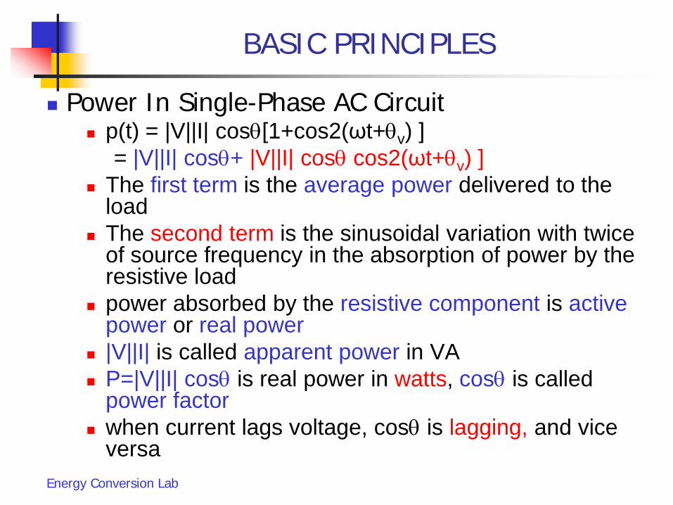
Power In Single-Phase AC Circuit p(t) = |V||I| cosθ[1+cos2(ωt+θv) ]

= |V||I| cosθ+ |V||I| cosθ cos2(ωt+θv) ] The first term is the average power delivered to the

load The second term is the sinusoidal variation with twice

of source frequency in the absorption of power by the resistive load

power absorbed by the resistive component is active power or real power

|V||I| is called apparent power in VA P=|V||I| cosθ is real power in watts, cosθ is called

power factor when current lags voltage, cosθ is lagging, and vice

versa

Energy Conversion Lab

BASIC PRINCIPLES

Power In Single-Phase AC Circuit pX(t) = |V||I| sinθsin2(ωt+θv), This term is the power oscillating into and out

of load of reactive element (capacitive or inductive)

Q=|V||I| sinθ is the amplitude of reactive power in “var” (voltage-ampere reactive)

For inductive load, current lagging voltage, θ= (θv-θi) > 0, Q is positive

For capacitive load, current leading voltage, θ= (θv-θi) < 0, Q is negative

Energy Conversion Lab

BASIC PRINCIPLES

The Instantaneous Power Has Some Characteristics For a pure resistor, cosθ=1, apparent power |V||I| =

real power In a pure inductive or capacitive circuit, cosθ=0, no

energy change but the instantaneous power oscillatebetween circuit and source

When pX(t) > 0, energy is stored in the magnetic field with the inductive elements, when pX(t) < 0, energy is extracted in the magnetic field with the inductive elements

If load is pure capacitive, the current leads voltage by 90o, average power is 0, vise versa for pure inductive load

Energy Conversion Lab

BASIC PRINCIPLES

Example 2.1(PSA-Saadat) supply voltage v(t)=100cosωt, inductive load Z=1.25∠60o Ω determine i(t), p(t), pR(t), px(t)

Energy Conversion Lab

COMPLEX POWER

The rms voltage phasor and rms current phasor V = |V|∠θv and I = |I| ∠θi The term VI* = |V||I| ∠(θv -θi) = |V||I| ∠ θ = |V||I| cosθ + j

|V||I| sinθ

Define a complex power quantity S = VI* = P + jQ, where The units of complex power S are kVA or MVA apparent power S is used as a rating unit of power

equipment apparent power S is used for an utility to supply power

to consumers

powerapparent ,22 QPS +=

θv

θi

V

Iθ

P

S Qθ

Energy Conversion Lab

COMPLEX POWER

Define a reactive power quantity Q Q is (+) when phase angle θ is (+), i.e. load is inductive. Q is (-) when

load is capacitive

Given a load impedance Z V=ZI S=VI*=ZII*= (R+jX)II* = (R+jX)|I|2 S=VI*=V(V/Z)*=V(V*/Z*)=(VV*)/Z*=|V|2/Z* Z=|V|2/S*

Complex power balance real power supplied by source = real power absorbed by load see Example 2.2 (PSA-Saadat)

θi

θv

V

I

θθ

P

SQ (-)

capacitive

Energy Conversion Lab

POWER FACTOR CORRECTION AND COMPLEX POWER FLOW

Apparent Power |S| > P if power factor (p.f.) < 1 current supplied in p.f. < 1 will be larger than current supplied in

p.f. = 1 a larger current will cost more!

Power factor inductive load causes lagging current and result in a lagging

power factor (p.f. < 1) , Z=jX, I=V/(jX)=(V/X) ∠-90o (lagging) capacitive load causes leading current and result in a leading

power factor (p.f. < 1), Z=-jX, I=V/(-jX)=(V/X) ∠+90o (leading) resistive load has a unity power factor (p.f. = 1)

To keep p.f. ≈ 1, we need to install capacitor banks through the network for inductive load industry probably operate at low lagging p.f. since most of them

are motors (inductive load) to correct low power factor, capacitor banks are connected in

parallel to the load for p.f. correction, see Ex. 2.3 in pp.23, Ex. 2.4 in pp.24 (PSA-

Saadat)

Energy Conversion Lab

COMPLEX POWER FLOW Complex power flow (PSA-Saadat)

see Figure 2.9 in pp. 26 complex power S12

real power at the sending end

reactive power at the sending end

2121

21

12 δδγγ −+∠−∠=ZVV

ZV

S

)cos(cos 2121

21

12 δδγγ −+−=ZVV

ZV

P

)sin(sin 2121

21

12 δδγγ −+−=ZVV

ZV

Q

V1∠δ1V2∠δ2

Z∠γ

Energy Conversion Lab

COMPLEX POWER FLOW OBSERVATION Observation on complex power flow

assume transmission lines have small resistance compared to the reactance (Z=X∠90o, cosγ=0), P12and Q12 becomes

maximum power occurs at δ = 90o, where maximum power transfer: Pmax=|V1||V2|/X

real power flow P12 could be changed by small change in δ1 or δ2

reactive power Q12 is determined by terminal voltage difference, (i.e., Q≒|V1|-|V2|)

line loss = S12 + S21 (PSA-Saadat)

( )( )21211

12

2121

12

cos

)sin(

δδ

δδ

−−=

−=

VVXV

Q

XVV

PV1∠δ1

V2∠δ2

Z∠γ

Energy Conversion Lab

COMPLEX POWER FLOW OBSERVATION Ex. 2.6 direction of power flow between two voltage

sources voltage source 1 can change phase from ±30o in step of 5o

phase of voltage source 2 is constant

Energy Conversion Lab

PROJECT 2 Two voltage of sources V1=120∠-5 V rms and V2=100∠0 V

rms are connected by a short line of impedance Z=1+j7 Ω. The figure is shown below

Write a Matlab program such that the voltage magnitude of the source 1 is changed from 75% to 100% of the give in steps of 1V. The voltage magnitude of source 2 and phase angle are kept constant. Compute the complex power for each source and the line loss. Tabulate the reactive powers and plot Q1, Q2, and QL versus voltage magnitude |V1|.

From the results, show that the flow of reactive power along the interconnection is determined by the magnitude difference of the terminal voltages.

V1∠δ1V2∠δ2

Z∠γ

Transmission Line Modeling

Derivation of Terminal V,I relations Transmission matrix Transmission line circuit equivalent Complex power transfer (short line) Complex power transmission

short radial line Complex power transmission

long or medium line Power handling capability

SHORT LINE MODEL Short line model assumption

length shorter than 80km/50 miles, voltage < 69kV capacitance is ignored line is represented with series RL circuits

Equivalent short line model is shown as below

Phase voltage at sending end: VS=VR+ZIR Phase current in the short line: IS=IR For steady state transmission equations, sending ends V,I in terms

of receiving ends

Z=R+jX+

-VS VR

+

-

SR

IS IR

=

=

R

R

R

R

S

S

IV

TIVZ

IV

1 0 1

=

1 0Z 1

T

SHORT LINE MODEL For steady state transmission equations, receiving ends V,I in terms

of sending ends

For short line (line length<80km/50mi) Series RL circuit model, no shunt admittance

Voltage regulation of the line

Transmission line efficiency

=

−

=

−

S

S

S

S

R

R

IV

TIV

ACBD

IV 1

-

lLjrlIVZ

IV

R

R

S

S )(zZ ,1 0

1ω+==

=

100 )(

)()( ×−

=FLR

FLRNLR

VVV

VRPercent

)3(

)3(

φ

φηS

R

PP

=

MEDIUM LINE MODEL When length>80km (50miles), line charging current becomes

appreciable and shunt capacitance must be considered To consider the shunt capacitance, half of the shunt capacitor may

be lumped at each end of line The referred shunt circuit is called the nominal π model

Y is the total shunt admittance of line with length l: Y=(g+jωC)*l Derivation of the shunt circuit matrix

From KCL, ,

from KVL the sending end voltage: We have VS in terms of receiving end variables:

RRL VYII2

+=

LRS ZIVV +=

RRS ZIVZYV +

+=

21

VS VRY/2 Y/2

R jXIS IR

IL

MEDIUM LINE MODEL

Derivation of the shunt circuit matrix The sending end current: We have IS in terms of receiving end variables:

For medium line, nominal π circuit model

In general, the medium line matrix, ABCD have complex constants and symmetrical with A=D, and AD-BC=1

SLS VYII2

+=

RRS IZYVZYYI

++

+=

21

41

yllIV

ZYZYY

ZZY

IV

R

R

S

S ==

++

+=

Y,zZ ,

21 )

41(

2

1

Energy Conversion Lab

DERIVATION OF V,I RELATIONS From Kirchhoff’s voltage law, taking limit as Δx -> 0

From Kirchhoff’s current law, taking limit as Δx -> 0

)()()(

)()()(

xzIx

xVxxVor

xxIzxVxxV

=∆

−∆+∆+=∆+

)()( xzIdx

xdV=

)()()(

)()()(

xyVx

xIxxIor

xxVyxIxxI

=∆

−∆+∆+=∆+

)()( xyVdx

xdI=

DERIVATION OF V,I RELATIONS Second order V equation is

General solution is:

where is characteristic impedanceis the propagation constant

γ=α+jβ, α is attenuation constant, β is phase constant For a desired load voltage or complex power is specified, we can

use this equation to calculate supply side variables to satisfy its loads

Under normal operation, a power system is driven by the demand of loads

IyzIdx

Id

VyzVdx

Vd

22

2

22

2

γ

γ

==

==

ll

lIlVV RRS

γγ

γγ

sinhZV coshII

sinhZ cosh

c

RRS

c

+=

+=

yzZc /=

zy=γ

TRANSMISSION MATRIX Arrange V,I equations in matrix form

The transmission parameters A,B,C,D form the transmission matrix T

where

Therefore,

As before, A=D and AD-BC=1 If we want to calculate V,I from sending end to

receiving end. Just simply use T-1

=

DC BA

T

RRc

cR

Ix coshVx sinhZ1 )(

Ix sinhZVx cosh)(

γγ

γγ

+=

+=

xI

xV R

x cosh Dx, sinhZ1C

x sinhZ Bx, coshA

c

c

γγ

γγ

==

==

=

=

R

R

R

R

IV

TIV

DCBA

xIxV

)()(

LUMP-CIRCUIT EQUIVALENT

The π equivalent circuit for transmission line

We end up with the solution

Z’

Y’/2 Y’/2V1 VR

I1 IR

R

RR

IYZVYZY

IZ'VYZV

)2

''1( )4

''1('I

)( )2

''1(

R +++=

++=

++

+=

R

R

IV

YZYZY

Z'YZ

IV

2''1 )

4''1('

2

''1

LONG LINE LUMP-CIRCUIT

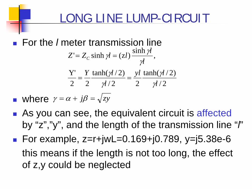
For the l meter transmission line

where As you can see, the equivalent circuit is affected

by “z”,”y”, and the length of the transmission line “l” For example, z=r+jwL=0.169+j0.789, y=j5.38e-6

this means if the length is not too long, the effect of z,y could be neglected

2/)2/tanh(

22/)2/tanh(

22Y'

, sinh )z( sinh'

llyl

llY

llllZZ C

γγ

γγ

γγγ

==

==

zyj =+= βαγ

REVIEW FOR SIMPLIFIED MODELS

For steady state transmission equations, sending endsV,I in terms of receiving ends

For steady state transmission equations, receiving ends V,I in terms of sending ends

=

=

R

R

R

R

S

S

IV

TIV

DCBA

IV

=

DC BA

T

=

−

=

−

S

S

S

S

R

R

IV

TIV

ACBD

IV 1

-

REVIEW FOR SHORT, MEDIUM LINE MODELS

If |rl|<<1,

For short line (l<50mi)Series RL circuit model

no shunt admittance

For medium line (50<l<150 mi, approximately)Nominal π circuit model, shunt admittance becomes more apparent

222/)2/tanh(

22Y' ,

rr sinh )z(' ylY

rlrlYzlZ

lllZ ======

lIVZ

IV

R

R

S

S zZ ,1 0

1=

=

yllIV

ZYZYY

ZZY

IV

R

R

S

S ==

++

+=

Y,zZ ,

21 )

41(

2

1

LONG LINE MODEL

For long line (l>150 mi, approximately)Use π equivalent circuit, contains trigonometric term and Z,Y parametersEquivalent π circuit model

2/)2/tanh(

22/)2/tanh(

22Y'

, sinh sinhzZ'

,

2''1 )

4''1('

' 2

''1

llY

llyl

llZ

lll

IV

YZYZY

ZYZ

IV

R

R

S

S

γγ

γγ

γγ

γγ

==

==

++

+=

Complex Power Transmission From steady-state V,I equations

The complex power transfer delivered to the receiving end can be computed from

For lossless line

=

=

R

R

R

R

S

S

IVZ

IV

DCBA

IV

1 0 1

*

*

)(

−

−=

−=+−=−

BAVVV

IVjQPS

RSR

RRRRRS

** )( RRSSSSSSR DICVVIVjQPS +==+=

Complex Power Transmission Complex power transfer from sending end to

receiving end

Calculate the complex power transfer from sending end

RSZj

jRR

jS

eZZ

eVeV RS

θθθ

ωθθ

−≡=

==

+=

∠SR

S

,

V ,VLjRZ Assume

SRjZjRSZjS

RSSSSSR

eeZVV

eZ

VZ

VVVIVS

θ∠∠ −=

−==

2

**

)(

Complex Power Transmission Complex power transfer from receiving end to

sending end

Calculate the complex power transfer from receiving end

RSZj

jRR

jS

eZZ

eVeV RS

θθθ

ωθθ

−≡=

==

+=

∠SR

S

,

V ,VLjRZ Assume

( )

SRjZjSRZjR

RSRRRRS

eeZVV

eZ

VZ

VVVIVS

θ−∠∠ +−=

−=−=−

2

**

)(

Power Circle Analysis Sending end circle and receiving end circle

Circles do not intersect if |VS|≠|VR| θSR increase will increase the complex power

transfer until ultimate limit For the transmission line

SRSR jRRS

jSSR BeCSBeCS θθ −+=−= - ,

ZVV

B

ZZ

VC

ZZ

VC

RS

RR

SS

=

∠−=

∠=

,

,

2

2

SRjZjRSZjSSR ee

ZVV

eZ

VS θ∠∠ −=

2

SRjZjSRZjRRS ee

ZVV

eZ

VS θ−∠∠ +−=−

2

COMPLEX POWER CIRCLE

)(2

ZZ

VS ∠

)(2

ZZ

VR ∠−ZjRS e

ZVV

radius ∠=

δ

sending end circle

receiving end circle

δ

P

Q

SRjZjRSZjSSR ee

ZVV

eZ

VS θ∠∠ −=

2

SRjZjSRZjRRS ee

ZVV

eZ

VS θ−∠∠ +−=−

2

SRRS θθθδ =−=∠

COMPLEX POWER FLOW

For lossless line, the real and reactive power transfer from sending end to receiving end B=jX, θA=0, θB=90o, A=cos βl

Power is transferred proportional to power angle δ, as load increases, δ increase

For lossless line, max power occurs when δ=90o, but for the adequate margin of stability, δ is between 30o to 45o

lX

VXVV

Q

XVV

PP

LLRLLRLLSSR

LLRLLSRSSR

βδ

δ

φ

φφ

coscos

sin

2

)()()()3(

)()()3()3(

−−−

−−

−=

=−=

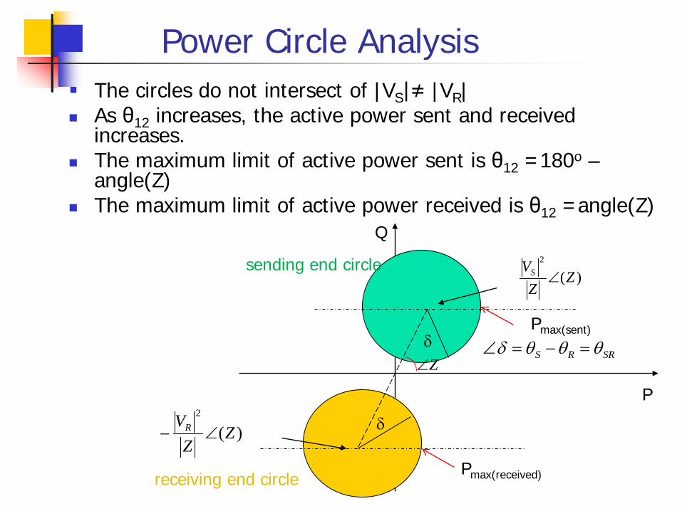
Power Circle Analysis The circles do not intersect of |VS|≠ |VR| As θ12 increases, the active power sent and received

increases. The maximum limit of active power sent is θ12 =180o –

angle(Z) The maximum limit of active power received is θ12 =angle(Z)

)(2

ZZ

VS ∠

)(2

ZZ

VR ∠−

δ

sending end circle

receiving end circle

δ

P

Q

SRRS θθθδ =−=∠Z∠

Pmax(sent)

Pmax(received)

NCKU EE Energy Conversion Lab. 92781

43.2315104.6636

loss S R

loss s R

P P P MWQ Q Q MVar

= − == − =

Power Circle Analysis

too much θSR increase will force synchronous machine running out of synchronism

How can we increase the ultimate transmission capability? Decrease X or increase |V|

Decrease X: line design (space, material) Increase |V|: sometimes not feasible For lossless line |VS| ≈ |VR|,|Z| ≈90o, θSR

<10o , PSR coupled with θSR , QSR coupled with |VS|-|VR|

POWER TRANSMISSION CAPABILITY

Power handling capability is limited by thermal loading: Sthermal=3VφratedIthermal

stability limit: load angle δ In practice, when generator and transformer are

connected to transmission line, the combined reactance will result in a larger δ for a given load

Power Handling Capability of Line

Thermal limit: line temperature to prevent line sag, irreversible stretching and insulation Bundling for greater spacing

Current limit: Thermal limit can affect current carrying Voltage limit: Conductor size, spacing and insulation MVA limit: MW and MVAr, typically a 345kV line has a

thermal rating of 1600MVA θSR limit: synchronism max limit between

40-50o, which is about 65 to 75% of the ultimate transmission capability

Power handling capability is limited by thermal rather than stability for short lines, vice versa for long lines

Project analysis (project 2-1)

Distributed Parameter Model The distributed parameter model states that

Let Δx -> 0, the above equation

xtvCGvxxixi ∆∂∂

+=∆+− )()()(

xtiLRixxvxv ∆∂∂

+=∆+− )()()(

tvCGv

xi

∂∂

+=∂∂

−

tiLRi

xv

∂∂

+=∂∂

−

I

( ) YVVCsGdxdI

−=+−=

( ) ZIILsRdxdV

−=+−=

Laplacetransform

Distributed Parameter Model

When the line is lossless, R and G are zero characteristic impedance

propagation speed of v and I along the line

Take the time derivative of the left equations

CL

iv=

∂∂

CLtx 1=

∂∂

IIsLRsCGdx

Id 22

2

))(( γ=++=

VVsCGsLRdx

Vd 22

2

))(( γ=++=

( ) YVVCsGdxdI

−=+−=

( ) ZIILsRdxdV

−=+−=

Distributed Parameter Model

The solution of the second order differential equation

Propagation constant characteristic impedance

Voltage component Vf=IfZc, Vb=-IbZc

V(x,s)= Vf+ Vb=Zc(If –Ib) For terminal impedance Zd

fb I

rx

I

rx eAeAsxI −+= 21),( bf V

rxc

V

rxc eAZeAZsxV 12),( −= −

bf

bfcd II

IIZsdIsdVsZ

+

−==

)(),(),()(

LCsLCR+=

2γ

)()(

sCGsLRZc +

+=

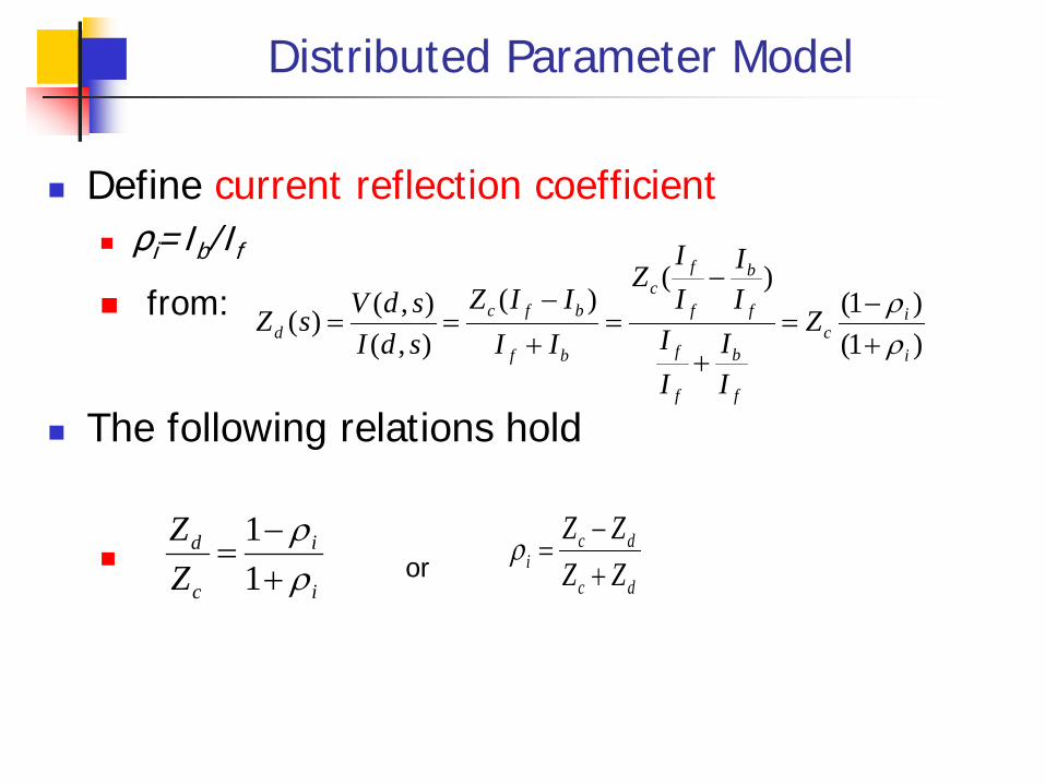
Distributed Parameter Model

Define current reflection coefficient ρi=Ib/If

from:

The following relations hold

or

)1()1(

)()(

),(),()(

i

ic

f

b

f

f

f

b

f

fc

bf

bfcd Z

II

II

II

II

Z

IIIIZ

sdIsdVsZ

ρρ

+−

=+

−=

+

−==

dc

dci ZZ

ZZ+−

=ρi

i

c

d

ZZ

ρρ

+−

=11

Distributed Parameter Model

Define voltage reflection coefficient ρv=Vb/Vf

ρi = - ρv

The reflection coefficients of some common terminations are:

∞=dZ 1=vρOpen-circuit 1−=iρ

Short-circuit

Matched termination

0=dZ

cd ZZ =

1−=vρ

0=vρ

1=iρ

0=iρ

dc

dc

Cf

Cb

f

bv ZZ

ZZZIZI

VV

+−

−=−

==ρ

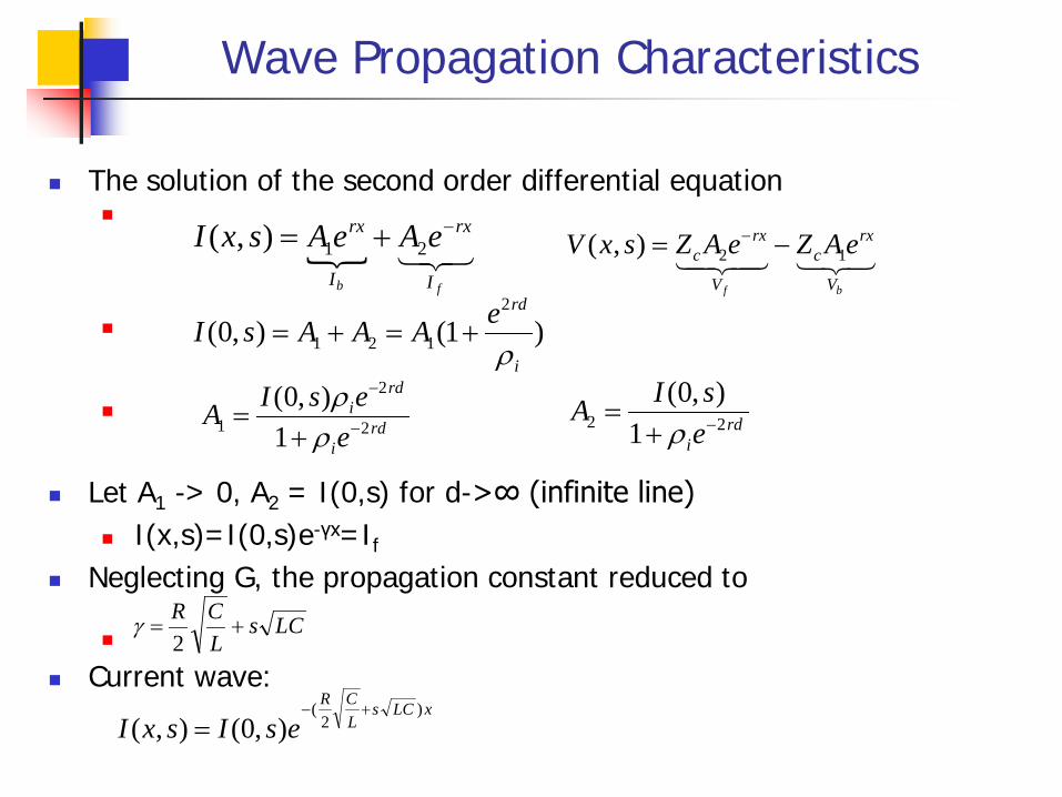
Wave Propagation Characteristics

The solution of the second order differential equation

Let A1 -> 0, A2 = I(0,s) for d->∞ (infinite line) I(x,s)=I(0,s)e-γx=If

Neglecting G, the propagation constant reduced to

Current wave:

fb I

rx

I

rx eAeAsxI −+= 21),(

bf V

rxc

V

rxc eAZeAZsxV 12),( −= −

)1(),0(2

121i

rdeAAAsIρ

+=+=

rdi

rdi

eesIA 2

2

1 1),0(

−

−

+=

ρρ

rdie

sIA 22 1),0(−+

=ρ

xLCsLCR

esIsxI)

2(

),0(),(+−

=

LCsLCR+=

2γ

Distributed Parameter Model

Transient wave propagation characteristics, for ∞ long line

atten. Factor delay

The time-domain response of the forwarding voltage

V,I reflection coefficients, ρv, ρi

Simulation of a single-phase line

)(),0(),()

2(

xLCtuxLCtietxix

LCR

−−=−

),(),( txiZtxv C=

The Bewley Lattice Diagram V is applied at t=0 to a line of length d, characteristic impedance

ZC that is terminated with an impedance Zd at the other end Assume the source impedance at the sending end is zero, i.e., ρvs

= -1 The bewley lattice diagram is as follows

Simulation of A Single-phase Line Source circuit Load circuit

State variable: vbs, vfR

forward, backward wave relations:

sending end and receiving end relations

dtdiLiRve S

SSSS +=−

∫ −= dtiRvL

i RLRL

R )(1∫ −−= dtiRve

Li SSS

SS )(1

bsSCS viZv 2+= RCfRR iZvv −= 2

fRRbR vvv −=bsSfs vvv −=

)( ),()

2(

xLCtuvetxv fs

xLCR

fR −=−

)( ),()

2(

xLCtuvetxv bR

xLCR

bs −=−

Distributed Parameter Model

Line model)( ),(

)2

(xLCtuvetxv fs

xLCR

fR −=−

)( ),()

2(

xLCtuvetxv bR

xLCR

bs −=−

Distributed Parameter Model

Single phase line simulation

Project 3

A transmission system with a supply source at sending end in rated voltage 500 kV, 60Hz. The 1000km single phase line has the following electrical parameters R = 0.15 Ω/km, L=2.96 mH/km C=0.017 µF/km

with 1000 km long line. The source electrical parameters are: RS=50 Ω,

LS=0.1H

Now the transmission line is connected to a single phase RL load of RL=5.4kΩ, LL=10.743H

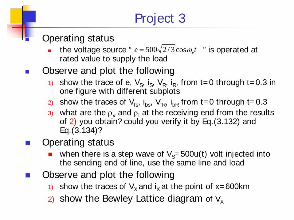
Project 3 Operating status

the voltage source “ ” is operated at rated value to supply the load

Observe and plot the following1) show the trace of e, VS, iS, VR, iR, from t=0 through t=0.3 in

one figure with different subplots2) show the traces of Vfs, ibs, VfR, ibR from t=0 through t=0.33) what are the ρv and ρi at the receiving end from the results

of 2) you obtain? could you verify it by Eq.(3.132) and Eq.(3.134)?

Operating status when there is a step wave of VS=500u(t) volt injected into

the sending end of line, use the same line and load Observe and plot the following

1) show the traces of VX and iX at the point of x=600km2) show the Bewley Lattice diagram of VX

te eωcos3/2500=