Creative Components Iowa State University Capstones, Theses and Dissertations

Spring 2020

Basic Principles of Genetic Gain and Feasibility of On-farm Basic Principles of Genetic Gain and Feasibility of On-farm

Estimation Estimation

Kenan Layden

Follow this and additional works at: https://lib.dr.iastate.edu/creativecomponents

Part of the Plant Breeding and Genetics Commons

Recommended Citation Recommended Citation Layden, Kenan, "Basic Principles of Genetic Gain and Feasibility of On-farm Estimation" (2020). Creative Components. 523. https://lib.dr.iastate.edu/creativecomponents/523

This Creative Component is brought to you for free and open access by the Iowa State University Capstones, Theses and Dissertations at Iowa State University Digital Repository. It has been accepted for inclusion in Creative Components by an authorized administrator of Iowa State University Digital Repository. For more information, please contact digirep@iastate.edu.

Basic Principles of Genetic Gain and Feasibility of On-farm Estimation By

Kenan Layden

A creative component submitted to the graduate faculty

in partial fulfillment of the requirements for the degree of MASTER OF SCIENCE

Major: Plant Breeding

Program of Study Committee:

Dr. William Beavis, Major Professor Dr. Thomas Lubberstedt

Iowa State University Ames, Iowa

2020

1

Table of Contents INTRODUCTION………………………………………………………………………………………………………………………………….3

Rationale…………………………………………………………………………………………………………………………………………………3

Objectives……………………………………………………………………………………………………………………….………………………6

BACKGROUND…………………………………………………………………………………………………………………………………….6

Galton and Regression……………………………………………………………………….……………………………………………………6

Mathematical Models for Quantitative Inheritance…………………………………………….…………………………………10

Lush and Genetic Gain……………………………………………………………………………………………………………………………13

Infinitesimal Model and Variance…………………………………………………………………………………………….……………16

MODELING AND ESTIMATION OF FIXED AND RANDOM EFFECTS………………….………………..…………….…..17

Mixed Model………………….………….………………………………………………………………………………………….………………17

Methods for Estimation of Quantitative Genetic Parameters.………………….……………………………………………18

ESTIMATION OF GENETIC TRENDS IN PLANT BREEDING AND AGRONOMIC PRODUCTION………………...19

Types of Genetic Trend Estimates Used in Plant Breeding……………………………………………………………………..19

Potential for On-Farm Estimation of Genetic Trends……………………………………………………………………………..23

SUMMARY …………………………………………………………………………………………………………………………………….…30

APPENDICES …………………………………………………………………………………………………………………………………….35

Appendix A: Quantitative Plant Breeding Basics ……………………………………………………………………………………35

Appendix B: ANOVA ……………………………………………………………………………………………………………………………..36

Appendix C: Linear Regression to Estimate Heritability ……………………………………………………………………..….39

Appendix D: Mixed Models ………………………………………………………………………………………………………………..…41

Appendix E: Experimental Practices and Field-Plot Design …………………………………………………………………….42

Appendix F: Model for On-Farm Genetic Trend Estimation …………………………………………………………………..47

GLOSSARY ………………………………………………………………………………………………………………………………………..49

BIBLIOGRAPHY……………………………………………………………………………………………………………………………….…54

2

Acknowledgements

I would like to thank Dr. Beavis for serving as my advisor and helping me to develop a creative

component which connects my educational work to plant breeding. The time spent helping develop my

ideas is greatly appreciated. I would like to thank Dr. Lubberstedt for serving on my committee. I would

also like to thank all the faculty and staff of the Plant Breeding Distance Education Program. Over the

past seven years they have facilitated learning and application of material and assisted me in navigating

the program with the change’s life brings. I would also like to thank Brett Peterson, Greg Endres, and

Mark Liebig for sharing ideas and research material from across North Dakota. A special thanks to my

agronomy mentor Josh Messer for continually helping me learn and explore possibilities within the plant

sciences. Thanks to Sandi Bates for sharing her literary expertise. Finally, I would like to thank all my

friends and family for supporting me through my distance education journey, especially my wife Kelly.

3

INTRODUCTION

Rationale

Many individuals working in the agriculture sectors of crop production and agronomy encounter

plant breeding and plant breeding concepts through their careers and educational experiences. Within

the State of North Dakota, agronomy and crop production students graduating with two-year Associates

in Applied Science degrees are not exposed to any statistical or plant breeding courses. Agronomy

students within the State of North Dakota graduating with a four-year Bachelor of Science degree are

required to take an introductory statistics course and introductory plant breeding course. Many

students who work producing crops upon graduation elect for other university majors in the areas of

agribusiness, agricultural economics, livestock production, or soil science. These majors generally

require an introductory statistical course, but not a plant breeding course. However, the crops that this

demographic grows on a year to year basis are the result of plant breeding.

The advent of modern genetics and application of mathematical principles to plant breeding

have led to development of crops in production that are of higher economic value. Improvement of

genotypic value has occurred in yield, seed composition, forage quality, tolerance to abiotic and biotic

stress, and adaptability to mechanization. Crops of high economic value are grown under a wide variety

of conditions. Crops will encounter different climatic conditions, cultural field practices, abiotic

stressors, and biotic stressors. These differing conditions and management practices used in the

cultivation of the crop can be referred to as the environment or non-genetic factors. Economically

important phenotypic traits observed in these crops are a result of genetic and environment

interactions. The goal of plant breeding is to produce cultivars that have genetically improved traits for

4

commercial producers (Fehr, 1991; Duvick et al., 2010). Producers are located across a range of

environments and they apply a range of management practices to produce crops. Plant breeders

identify limitations of current cultivars within specific environments and production systems and adapt

the crops to these conditions through genetic improvement and adaptation. Genetic changes generally

impart one of the following advantages: tolerance to abiotic and biotic stressors, tolerance to limiting

climatic factors, improvement of agronomic characteristics, changes that cause efficient yield

production within cultural production systems, and stabilizing traits for optimum growth under various

cultural production systems (Duvick et al., 2010; Graybosch et al., 2014; Hulke et al., 2014; Vandemark

et al., 2014).

Plant breeders predict and assess the improvement in average genetic value of a population

with each cycle of selection. This concept is termed genetic gain from selection (Lush & Hazel, 1942).

Genetic gain is the response to selection for additive genetic variance (Lush, 1945). Plant breeders

estimate predicted genetic gain periodically to compare the efficiency of different breeding strategies

and to evaluate the effectiveness of breeding programs (Hallauer et al., 2010; Rutkoski, 2019a). Plant

breeders also assess realized genetic gain. The estimation of realized changes in genotypic values over

multiple cycles or years is referred to as realized genetic gain or genetic trend (Rutkoski, 2019a, 2019b).

Many crop producers, despite their career paths and educational backgrounds, are not familiar with the

concepts of predicted and realized genetic gain or genetic trend along with how these terms are

associated with new cultivar releases for crops grown in their production operations. Crop producers are

the customers of the final product, the commercial cultivar, produced by a plant breeding operation.

Many crop producers are currently in a production situation where their profit margins are

smaller than 10 years ago. Costs associated with crop production have remained high or increased,

while revenue from crops per unit are similar to prices (unadjusted for inflation) producers received for

their products from 1980 to 2005. In order to increase profits, many crop producers seek to cut costs or

5

increase revenues from increased crop production or premium prices. Input from crop producers who

understand basic processes of crop improvement by local plant breeders may lead to identification of

crop characteristics that can be improved for premium prices or crops that rely on less costly inputs. By

providing products better suiting the need of crop producers, more success may be found by plant

breeding programs within the market.

Lower margins have also created the need for many crop producers to create on-farm test sites.

These sites allow for the comparison of different crop varieties and non-genetic inputs and management

practices. The sites allow farmers to evaluate proposed changes that will provide them with more

profitable operations. Note that farm sites are large and are planted and harvested with large scale

equipment (J. Messer, personal communication, January 17, 2020). The existence of on-farm research

sites provides an opportunity to estimate on-farm genetic gains. This estimation could create a decision-

making tool for crop producer to use when purchasing cultivars. The ability to compare the potential

genetic improvement component of traits and the increased cost of a new cultivar to a currently used

cultivar would benefit crop producers because it will help them assess claims of seed producers. My

personal conversations with producers about the cultivars used over the history of their production

operations elicit strong opinions on reliability of claims by the company selling the cultivar. Traditionally,

land grant universities and their extension services have served as independent evaluators of released

cultivars. In recent years, funding cuts to university extension services and non-participation by seed

companies have limited university extension services. On-farm estimation of genetic gain would allow

crop producers to generate objective results that used to be provided by universities, with the added

benefit of providing on-site relevancy to the results.

6

Objectives

The purpose of this manuscript is to communicate how rate of genetic gain per year could be

estimated on a crop production-farm. The paper will discuss a general background of what genetic gain

is, how realized genetic gain is currently estimated in crop breeding programs for one cycle of selection,

and how genetic trends are used to estimate genetic gain per year. The adaptation of current methods

of field plot experiments and designs to obtain estimates of genetic trend for a crop production

operation will be explored.

The second objective of this manuscript is to serve as a resource for crop producers I work with

in understanding the basic components of genetic gain and how plant breeding professionals may use

this concept. The general background on what genetic gain is and how it is estimated in both short and

long term will allow crop producers to acquire language commonly used by plant breeders leading to

greater understanding and better decision making for both crop producers and plant breeders.

BACKGROUND

Galton and Regression

In 1859 Charles Darwin published his book On the Origin of Species. His mechanism for evolution

is by the process of natural selection. Some of the main ideas of natural selection is that variation exists

within populations and is heritable. This variation can confer increased ability of some individuals to

produce viable progeny. Populations are continuously changing as selection acts on heritable variation.

During the years following the publication of On the Origin of Species, there was much debate within the

scientific community on where variation originates, what confers this variation, and if variation could

lead to continuous variability (Provine, 1971). In the early 20th century Gregor Mendel’s work on

inheritance was rediscovered and provided a theoretical explanation for the source of heritable

variation of continuous traits (Fisher, 1918; Wright 1920, 1921a, 1921b, 1921c, 1921d, 1921e) and how

7

the variation could explain evolution of continuous traits (Fisher, 1928a, 1928b; Wright, 1929). The

integration of Mendelian heredity and Darwinian selection became known as the Modern Synthesis and

the disciplines of population and quantitative genetics emerged as fundamental tools used by plant and

animal breeders.

Francis Galton observed the nature of many continuous traits. He was a cousin of Darwin and

did not believe evolution could happen continuously by natural selection (Provine, 1971). Much of

Galton’s work does not seek to explain the mechanism of inheritance but seeks to provide a measure of

quantitative inheritance (Magnello, 1998). Galton’s idea of measuring quantitative inheritance is a

necessary first step for developing models to estimate and predict inheritance of variants. Appendix A

contains further information on mathematical models and how they are utilized in plant breeding.

Galton’s contributions to the current estimates of genetic gain include the idea that variation can be

maintained within a population, reversion of offspring to population mean, and the use of regressions to

analyze inheritance.

Galton showed variation will remain within the population when randomly mated. In his book

Natural Inheritance (1889), Galton gave examples of continuous traits, such as human height or seed

size, having normal distribution within a population. Galton explained the continuous nature of traits

observed in an individual using the early Mendelian idea of inheritable particles, which would later be

referred to as genes (Lush, 1945). When random mating occurs, offspring receive particles (genes)

independently and randomly from parents. The sum of many independently inherited particles

constitutes the genetic makeup of an individual. In his paper Regression Towards Mediocrity in

Hereditary Stature (1886), Galton noted the plant seed size continued to have variation that was

different from the parental seed when randomly mated. Small seeds may have offspring with large

seeds, large seeds may produce small seeds. Galton explained this conservation of variation he observed

using the idea of random, independent inheritance of particles. This concept of inheritable particles

8

(genes) allows family likeness and individual variation to be attributed to the same cause. Three

instances may occur: individuals inherit elements from parents that will cause them to look like parents,

they will not inherit all elements causing variation and they will inherit latent characteristics that were

dormant in parents that will cause variation (Galton, 1889; Bulmer 1998).

Another important concept explored by Galton was the reversion of offspring to the population

mean. Galton showed when comparing offspring traits with parental traits, traits in the offspring tend to

revert to the population mean rather than parental mean. In Regression Towards Mediocrity in

Hereditary Stature (1886) and Natural Inheritance (1889), Galton demonstrated when regressing

standardized heights of children to the mid-parent value, child height tends to be closer to the

population average than the mid-parent height. Figure 1 simulates data showing this concept. The first

significant note here is Galton is the first to use a linear regression in a genetic context. The associated

regression model associated independent and dependent variables. The second significant note is

offspring tend to revert to the population mean. Galton explained the regression towards the mean of

normally distributed continuous traits using the same idea of independent, randomly inherited

elements. Since the trait values of many individuals are close to the center of the distribution for a trait,

there are more elements available to be passed on to offspring that will confer mean values. With more

available elements, more offspring will receive combinations of particles that confer the mean value for

a trait, thus the population will remain normally distributed around the same mean. Vice versa is true

for elements that lie far away from the mean. Being at a smaller frequency, there will be less elements

and combinations of elements that create values that lie far away from the mean (Galton, 1889).

Galton’s explanation for regression to the mean was not accurate; however, the concept that children

do not inherit all of the variation of the parents and reverted to the population mean was important in

the development of the of the mathematical model used today to describe genetic variance including

additive, dominance, and epistatic components of variance.

9

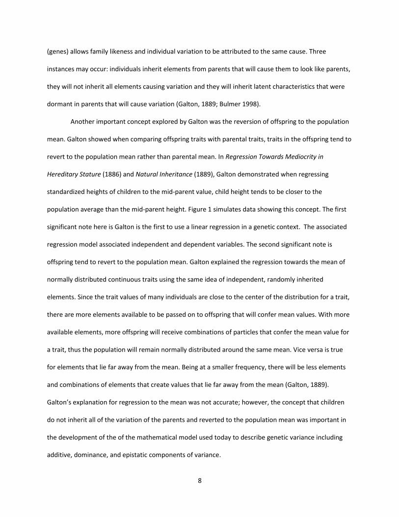
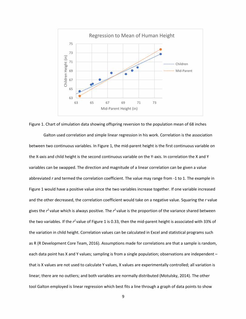
Figure 1. Chart of simulation data showing offspring reversion to the population mean of 68 inches Galton used correlation and simple linear regression in his work. Correlation is the association

between two continuous variables. In Figure 1, the mid-parent height is the first continuous variable on

the X-axis and child height is the second continuous variable on the Y-axis. In correlation the X and Y

variables can be swapped. The direction and magnitude of a linear correlation can be given a value

abbreviated r and termed the correlation coefficient. The value may range from -1 to 1. The example in

Figure 1 would have a positive value since the two variables increase together. If one variable increased

and the other decreased, the correlation coefficient would take on a negative value. Squaring the r value

gives the r2 value which is always positive. The r2 value is the proportion of the variance shared between

the two variables. If the r2 value of Figure 1 is 0.33, then the mid-parent height is associated with 33% of

the variation in child height. Correlation values can be calculated in Excel and statistical programs such

as R (R Development Core Team, 2016). Assumptions made for correlations are that a sample is random,

each data point has X and Y values; sampling is from a single population; observations are independent –

that is X values are not used to calculate Y values, X values are experimentally controlled; all variation is

linear; there are no outliers; and both variables are normally distributed (Motulsky, 2014). The other

tool Galton employed is linear regression which best fits a line through a graph of data points to show

63

65

67

69

71

73

75

63 65 67 69 71 73

Ch

ildre

n H

eigh

t (i

n)

Mid-Parent Height (in)

Regression to Mean of Human Height

Children

Mid-Parent

10

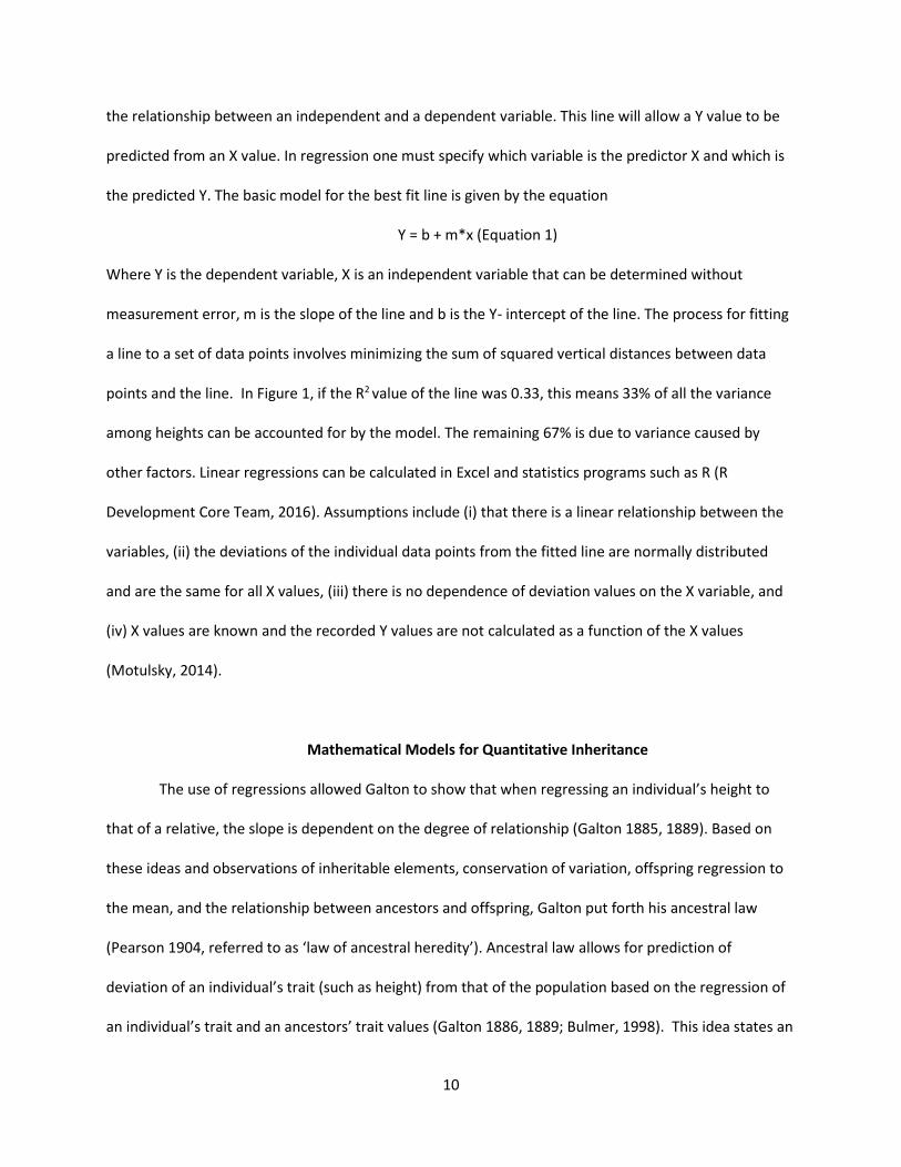
the relationship between an independent and a dependent variable. This line will allow a Y value to be

predicted from an X value. In regression one must specify which variable is the predictor X and which is

the predicted Y. The basic model for the best fit line is given by the equation

Y = b + m*x (Equation 1)

Where Y is the dependent variable, X is an independent variable that can be determined without

measurement error, m is the slope of the line and b is the Y- intercept of the line. The process for fitting

a line to a set of data points involves minimizing the sum of squared vertical distances between data

points and the line. In Figure 1, if the R2 value of the line was 0.33, this means 33% of all the variance

among heights can be accounted for by the model. The remaining 67% is due to variance caused by

other factors. Linear regressions can be calculated in Excel and statistics programs such as R (R

Development Core Team, 2016). Assumptions include (i) that there is a linear relationship between the

variables, (ii) the deviations of the individual data points from the fitted line are normally distributed

and are the same for all X values, (iii) there is no dependence of deviation values on the X variable, and

(iv) X values are known and the recorded Y values are not calculated as a function of the X values

(Motulsky, 2014).

Mathematical Models for Quantitative Inheritance

The use of regressions allowed Galton to show that when regressing an individual’s height to

that of a relative, the slope is dependent on the degree of relationship (Galton 1885, 1889). Based on

these ideas and observations of inheritable elements, conservation of variation, offspring regression to

the mean, and the relationship between ancestors and offspring, Galton put forth his ancestral law

(Pearson 1904, referred to as ‘law of ancestral heredity’). Ancestral law allows for prediction of

deviation of an individual’s trait (such as height) from that of the population based on the regression of

an individual’s trait and an ancestors’ trait values (Galton 1886, 1889; Bulmer, 1998). This idea states an

11

individual’s appearance is the result of declining contributions of inheritable elements from ancestors

that have a probability of being expressed each generation. Galton utilized a mathematical model to

predict height. The model is as follows:

D = ½ D1 + ¼ D2 + 1 8⁄ D3 +……... (Equation 2)

Where D is deviation of offspring from population mean, ½ is the contribution to offspring from mid-

parents, D1 is the deviation of the parent from the mean of the population, ¼ is the contribution to

offspring from mid-grandparent regression, D2 is the deviation of the grandparents from the mean of

the population, 18⁄ is the contribution to offspring from mid-great grandparent regression, and D3 is the

deviation of the great grandparents from the mean of the population (Provine, 1971). This calculation

could continue for as long as records of ancestors are kept.

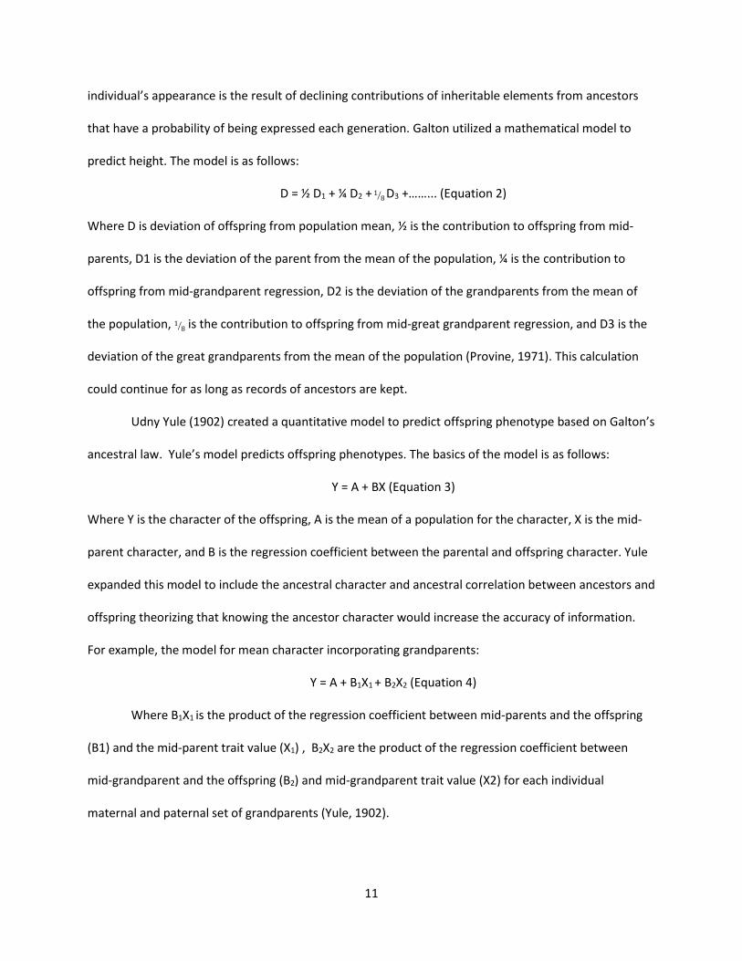
Udny Yule (1902) created a quantitative model to predict offspring phenotype based on Galton’s

ancestral law. Yule’s model predicts offspring phenotypes. The basics of the model is as follows:

Y = A + BX (Equation 3)

Where Y is the character of the offspring, A is the mean of a population for the character, X is the mid-

parent character, and B is the regression coefficient between the parental and offspring character. Yule

expanded this model to include the ancestral character and ancestral correlation between ancestors and

offspring theorizing that knowing the ancestor character would increase the accuracy of information.

For example, the model for mean character incorporating grandparents:

Y = A + B1X1 + B2X2 (Equation 4)

Where B1X1 is the product of the regression coefficient between mid-parents and the offspring

(B1) and the mid-parent trait value (X1) , B2X2 are the product of the regression coefficient between

mid-grandparent and the offspring (B2) and mid-grandparent trait value (X2) for each individual

maternal and paternal set of grandparents (Yule, 1902).

12

The models described by Galton (1889) and Yule (1902) assume a constant inheritable value can

be assigned to an individual from different generations and the standard deviations do not change from

generation to generation (Pearson, 1904). They also assumed their regression models, which regressed

offspring and parental values, accounted for all genetic variation. The rest of the variation in trait values

was thought to be due to the environment. When looking at the correlation of an individual between

the individual and their ancestors, Pearson (1904) noted the correlation coefficients calculated from

Galton’s data and regression correlations used by Galton and within Yule’s model were too small to

account for all genetic variation. Environment alone could account for all the additional variation

observed between parents and offspring. The correlation coefficients only explained a small portion of

variance observed within offspring of a set of parents. Yule’s model was missing parameters and

variables that accounted for environmental variation. This was a problem when reconciling Mendelian

principles and the continuous nature of traits. A mid-parent offspring regression could be used to

predict offspring values. However, it did not translate to a model that could account for all the genetic

variation within the offspring.

The work and personal communication of Galton, Yule, and Pearson lead Ronald A. Fisher to

develop a polygenic Mendelian model (Fisher, 1918; Hill, 2014; Barton et al., 2017). In his 1918 paper

Correlation Between Relatives on the Supposition of Mendelian Inheritance, Fisher showed as Pearson

(1904) did, that under the basic Mendelian principles genetic variance in children’s height cannot all be

attributed to inheritance from the parents. He cited the correlation coefficient value between brothers

is 54% and 46% of the variance must have other explanations. He showed the environment cannot alone

account for the remaining 46% of variation. Fisher mathematically showed how the variance of a set of

data can be used to partition out variance values for environment and genetic variance components.

Fisher further demonstrated genetic variance can be broken down into an additive component, a

dominance component, and an epistatic component. Based on this he portioned genetic variance into

13

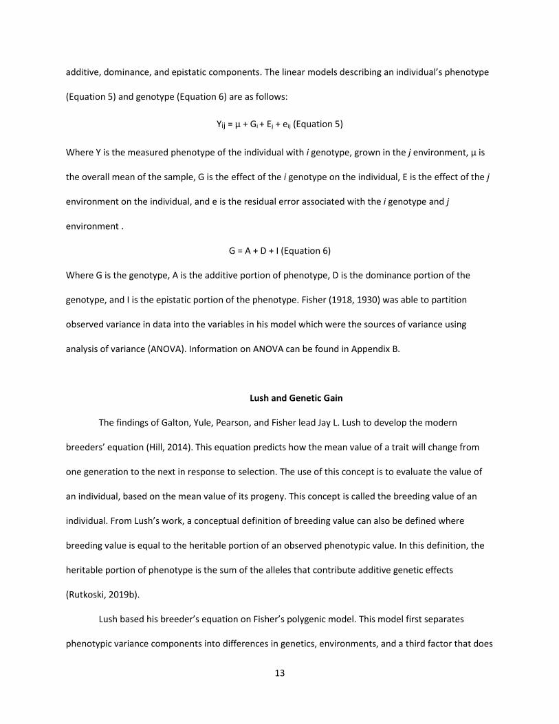
additive, dominance, and epistatic components. The linear models describing an individual’s phenotype

(Equation 5) and genotype (Equation 6) are as follows:

Yij = µ + Gi + Ej + eij (Equation 5)

Where Y is the measured phenotype of the individual with i genotype, grown in the j environment, µ is

the overall mean of the sample, G is the effect of the i genotype on the individual, E is the effect of the j

environment on the individual, and e is the residual error associated with the i genotype and j

environment .

G = A + D + I (Equation 6)

Where G is the genotype, A is the additive portion of phenotype, D is the dominance portion of the

genotype, and I is the epistatic portion of the phenotype. Fisher (1918, 1930) was able to partition

observed variance in data into the variables in his model which were the sources of variance using

analysis of variance (ANOVA). Information on ANOVA can be found in Appendix B.

Lush and Genetic Gain

The findings of Galton, Yule, Pearson, and Fisher lead Jay L. Lush to develop the modern

breeders’ equation (Hill, 2014). This equation predicts how the mean value of a trait will change from

one generation to the next in response to selection. The use of this concept is to evaluate the value of

an individual, based on the mean value of its progeny. This concept is called the breeding value of an

individual. From Lush’s work, a conceptual definition of breeding value can also be defined where

breeding value is equal to the heritable portion of an observed phenotypic value. In this definition, the

heritable portion of phenotype is the sum of the alleles that contribute additive genetic effects

(Rutkoski, 2019b).

Lush based his breeder’s equation on Fisher’s polygenic model. This model first separates

phenotypic variance components into differences in genetics, environments, and a third factor that does

14

not fit into the simple two-way division (genetic and environmental interactions; Equation 7). Lush did

not explicitly include genetic and environmental interactions in his model but did describe them in

writing. In a published work of his notes titled The Genetics of Populations, Lush (1948, 1994) notes in

addition to variation in environment and genetics there is “a residue or joint term which is a function of

their cooperation or antagonism, or of the nonlinearity with which their effects are combined.” The

genotypic component of variance then separates into additive, dominance, and epistatic contributions

of variance (Equation 8).

σPh2 = σG

2 + σE2 (Equation 7)

σG2 = σA

2 + σD2 + σI

2 (Equation 8)

Where σPh2 is the phenotypic variance, σG

2 is the genetic variance, σE2 is the environmental variance, σA

2

is the additive variance, σD2 is the dominance variance, and σI

2 is the epistatic variance. Lush was the first

to express of the genotypic variance components, only additive variance is transmissible to offspring and

should be used to estimate heritability of a trait from parent to offspring. This would mean only a

portion of the genotypic value determines the mean performance of the progeny and the breeding

value. Lush first shows this concept by discussing heritability in the broad sense (Equation 9). The

portion of phenotypic variance that is determined by genotypic variance components is given as:

σG2

__________ = σPh

2

σG2

____________ σG

2 + σE2

(Equation 9; Lush, 1945)

Where σPh2 is the phenotypic variance, σG

2 is the genotypic variance, and σE2 is the

environmental variance. This equation can be used to find a value of heritability if σG2 only consisted of

additive gene effects. Lush (1945, p. 100) notes that to find heritability “the formula would be correct if

the numerator were only the additive genetic portion of the variance.”

Based on this Lush showed the increase expected in a phenotypic population mean of offspring,

as a result of selection of parents when compared to parental generation before selection, is equivalent

15

to the selection differential if all gene effects were additive and environmental variations did not affect

the trait. In this case, the selection differential can be defined as the average performance of the

selected parents versus the population mean (Falconer & Mackay, 1996). If all gene effects are not

additive, the effect on the population mean from selection will be equivalent to a fraction of the

selection differential. This fraction will be equal to the narrow sense heritability (Equation 10).

h2=

σA2

_______________ = σph

2

σA2

___________________________ σA

2 + σD2 + σI

2 + σE2

(Equation 10; Lush, 1945)

Where h2 is narrow sense heritability, σA2 is the additive variance, σD

2 is the dominance variance, σI2 is

the epistatic variance, σE2 and environmental variance, and σPh

2 is the phenotypic variance. These

concepts can be written as the breeder’s equation, also known as predicted genetic gain:

R = h2S (Equation 11)

Where R is the response to selection, h2 is the narrow sense heritability, and S is the selection

differential. From this equation, response to selection can be defined as the difference in mean breeding

value (additive genetic effect) that occurred for one selection cycle (Rutkoski, 2019b).

Lush’s breeder’s equation can be used to predict response to selection, also known as predicted

genetic gain. Selection differential can be predicted given that genotypic variability is normally

distributed and truncation selection of the best individuals is conducted. For truncation selection no

individuals with a phenotypic value below the truncation point are retained for a new cycle of mating. If

these conditions are met, the selection differential is dependent on the portion of population that is

selected and the phenotypic standard deviation of the character. The selection can be estimated using

Equation 12. Where σph is the standard deviation of the phenotype and i is intensity of selection. The

intensity of selection is based on the proportion of population selected. It can be predicted from table

values (Falconer & Mackay, 1996, p. 379-380):

S = i σph (Equation 12; Falconer & Mackay, 1996)

16

The expected response from the breeder’s equation is given:

R=

i h2 σP =

i h σA =

i σA2

______________ σph

(Equation 13; Fehr, 1991; Falconer & Mackay, 1996)

Lush outlined methods for measuring heritability based on his breeder’s equation. The most

useful approach he used is the linear regression of parents to their offspring used for estimating

individual values for narrow sense heritability (Lush, 1940, 1994). Further detailed information on this

regression model can be found in Appendix C.

Infinitesimal Model and Variance

Lush’s work and development of the breeder’s equation focused on short-term improvement

and the selection of the best parents to breed for the next generation. Hill (2014) notes in short-term

improvement scenarios, finite populations, the magnitude of genetic effects, and epistasis do not affect

selection. These concerns are not present, if the infinitesimal model is assumed and many loci

contribute to a trait. In Animal Breeding Plans (1945), Lush acknowledged principles of the infinitesimal

model first described by Fisher (1918). When discussing the variability of a population he noted

selection has little effect on the amount of variability within a population. Variability may be altered

slightly by gene frequency changes and gamete arrangement (more intermediate combinations of

desirable and undesirable genes) from non-random mating. Lush noted when selection ceases and

random mating occurs, the reduction in variability caused by gametic rearrangements disappears

quickly. Bulmer (1971) presented a mathematical explanation of how gamete arrangement leads to no

lasting changes of the population variance. For no lasting changes of genetic variances to occur,

assumptions made to do this include that an infinite number of loci influence a phenotypic trait. This

assumption allows for no change in gene frequency through selection. With this restriction, the

17

reduction of variance of a mass selected group is due to gametic phase disequilibrium (covariances).

Genetic variance under selection is the sum of two components: genetic variance and disequilibrium

contribution. If a population randomly mates the covariance is zero. However, when mass selection and

non-random mating occur, pairs of loci that are correlated (are in gametic disequilibrium) will affect the

variance of the selected trait. The disequilibrium is what causes a negative covariance which causes a

decrease in genetic variance with selection, not an actual change in the genetic portion of variance.

When random mating occurs after selection, the disequilibrium is lost as joint equilibrium at pairs of loci

is restored. Any lasting change in variance due to selection must decrease the number of variable loci

affecting the trait (Bulmer, 1971). While not controlled by an infinite number of loci, quantitative traits

may be controlled by a very large number of loci preserving most of the variation within a population

where selection occurs.

MODELING AND ESTIMATION OF FIXED AND RANDOM EFFECTS

Mixed Model

Fisher developed the first linear mathematical model to explain quantitative genetic inheritance

and developed the ANOVA which allowed for isolation of quantitative genetic parameters such as

estimates of variance components (see Appendix B). These variance components can be used to

calculate narrow sense heritability which is used in the calculation of predicted genetic gain (Fehr,

1991). Lush utilized linear regression to estimate quantitative genetic parameters and genetic gain (see

Appendix C). ANOVA and linear regression are still used to estimate genetic parameters used to

calculate the predicted genetic gain. However, new procedures have been developed for estimation of

genetic parameters and estimation of fixed and random effects of individuals based on the linear mixed

model (for more information on fixed and random effects within models see Appendix B).

18

ANOVA can analyze linear models with both fixed and random effects. However, application of

least squares estimators of parameters in mixed models may encounter problems. Linear models used

for ANOVA, usually encounter issues when dealing with unbalanced data. Unbalanced data refers to

data classified multiple ways with different numbers of observations for certain factors. Measures of

effects of one factor depend upon other factors in the model (Littell, 2002). An example of unbalanced

data would include a specific genotype that was not evaluated in all environments. This means there will

be missing data in the analysis for these genotypes in these environments. In addition, the breeder may

have data from different years and have different locations between those years for genotypes thus

creating unbalanced data. Another problem in many plant and animal breeding programs, selection

occurs within the populations the breeder is analyzing. This violates the assumption of linear regression

and ANOVA that the sample population is randomly selected (Henderson, 1975).

Algorithms have been developed for linear mixed models to overcome the problems associated

with estimation of parameters using unbalanced data. One procedure of estimating fixed effects and

random effects within the linear mixed model is based on the work of or C.R. Henderson (Littell, 2002;

Hill & Kirkpatrick, 2010; Bernardo, 2020). Estimates of fixed effects are termed Best Linear Unbiased

Estimators or BLUE’s and estimates of random effects are termed Best Linear Unbiased Predictions or

BLUP’s. For more information on the linear mixed model refer to Appendix D.

Methods for Estimation of Quantitative Genetic Parameters

The procedures and statistical methods of Henderson’s mixed model rely on values of variances

and covariances of random effects and assume these values are known. The true values of genetic and

nongenetic variances are unknown in experimental data, so these variances must be estimated.

Restricted likelihood methods are often used to estimate genetic parameters such as genotypic

variances (Bernardo, 2020). Maximum likelihood (ML) methods seek to find the estimates of population

19

parameters that would give the greatest likelihood of the observed data. ML methods assume fixed

factors are known without error. This results in bias within variance estimates. ML methods estimate

variances are biased due to not adjusting the degrees of freedom. Restricted maximum likelihood

(REML) methods remove this bias by adjusting for degrees of freedom. REML methods maximize the

portion of the likelihood that does not depend on fixed effects (Hill & Kirkpatrick, 2010; Bernardo, 2020).

The basic idea is fixed effects are removed through a transformation. In a balanced design, least squares

estimators and REML estimators of variances and covariances are equivalent (Thompson, 2008).

Rex Bernardo (1994) was one of the first to apply mixed models to plant breeding. Bernardo

predicted the yield of hybrid crosses of maize from restriction length polymorphisms (RFLP) in the

parental lines potentially used for crosses and yield data from a set of related single crosses. RFLP was

used to define the coancestry (measure of genetic similarity) of crosses. REML methods were used to

estimate the genetic variances of hybrid cross due to the coancestry of parents. Once non genetic and

genetic variances were estimated, Bernardo then used REML to predict the performance of potential

hybrid crosses.

ESTIMATION OF GENETIC TRENDS IN PLANT BREEDING AND AGRONOMIC PRODUCTION

Types of Genetic Trend Estimates Used in Plant Breeding

The term genetic trend was introduced to distinguish realized genetic gains from predicted

genetic gains. Where the breeder’s equation is typically applied to data generated within a single cycle

of selection, genetic trends (realized genetic gains) estimate the realized changes in genotypic values in

two to multiple breeding cycles. If the genetic trend in linear, genetic gain per cycle that is realized can

be estimated by regressing the mean breeding value for a trait of interest. The slope of the regression

line is the estimate of realized genetic gain per cycle (Eberhart, 1964; Garrick, 2010; Rutkoski, 2019a,

2019b). In order to estimate genetic trends, cultivars must be grown in the field. Basic field-plot

20

techniques must be followed in order to isolate the genetic effects from non-genetic sources of

variability. These field-plot techniques utilize best practices for experimental designs which include

randomization, replication, blocking, and connectedness. Appendix E contains definitions and examples

of these experimental design concepts.

To date, two approaches have been used to estimate genetic trends. These approaches involve

either a balanced set of genotypes and management practices applied to each of several fields across

multiple years, where fields represent complete blocks, or an unbalanced set in which fields and years

are connected by a subset of genotypes and management practices, where each field represents a type

of incomplete connected block (Eccleston & Hedayat, 1974). A balanced factorial complete block

approach to trend estimation involves growing a few popular historical cultivars from each of regularly

spaced years in a common set of environments and regressing the cultivar averages against year

(Duvick, 1997, 2005; Smith et al., 2014; Rutkoski, 2019a, 2019b). This approach is generally referred to

as an era trial and methods were described and utilized by Donald Duvick in the estimation of realized

genetic gains in hybrid corn (1997, 2005).

Estimation using balanced factorial sets accounts for differences in management practices by

growing all cultivars using the set of management practices from the era when the popular cultivars

were grown. Thus, recent cultivars are grown under current management practices as well as historical

practices, while historical cultivars are likewise grown under all management practices. A limitation of

the method is the resources required to conduct the field trials. Duvick (1997) grew 36 hybrids, in three

locations, each hybrid was planted at three densities to adjust for historical management practices, but

he used small plots requiring investments in specially designed small plot planters, cultivators, and

combines. In order to implement the method using on-farm equipment would require a large amount of

field space. Another limitation associated with balanced factorial block experiments is the adjustment of

both old and new varieties to management practices associated with production practices of the era. An

21

example of this is observed in an era trial conducted by Cox et al. (1988) in which lodging scores were

recorded for all varieties because high nitrogen fertilizer rates were associated with greater lodging

rates among historical varieties.

Estimation of genetic trends using connected incomplete blocks involves collection of field data

over multiple years. For the plant breeders, the data utilized is sourced from field trials conducted

routinely as part of the cultivar development process. The data analyses utilize the linear mixed model

(see Appendix D) to isolate the genetic component from non-genetic sources of variability. Linear mixed

models account for unbalanced data and use algorithms such as REML that provide best linear unbiased

estimates (BLUE’s) of fixed effects and best linear unbiased predictions (BLUP’s) of random effects. Table

1 summarizes reviewed studies. The largest challenge for this approach is the possibility that not all

blocks (years and fields) will be connected by common cultivars or management practices. If some

cultivars are not replicated among years and fields, there is a lack of connectivity upon which to evaluate

non-genetic effects. A lack of connectivity may lead to the inability to separate the genetic and year

effects on a trait measured in a cultivar within the trial (Mackay et al., 2011; Rutkoski, 2019b).

In order to deal with this issue of confounding genotypic and annual effects, Mackay et al.

(2011) and Piepho et al. (2014) proposed only varieties that are connected for at least three years. In

addition, linear mixed models developed by Mackay et al. (2011) and Piepho et al. (2014) modeled years

and genotypes as fixed effects. Other factors such as environment and interactions of factors were

modeled as random effects.

22

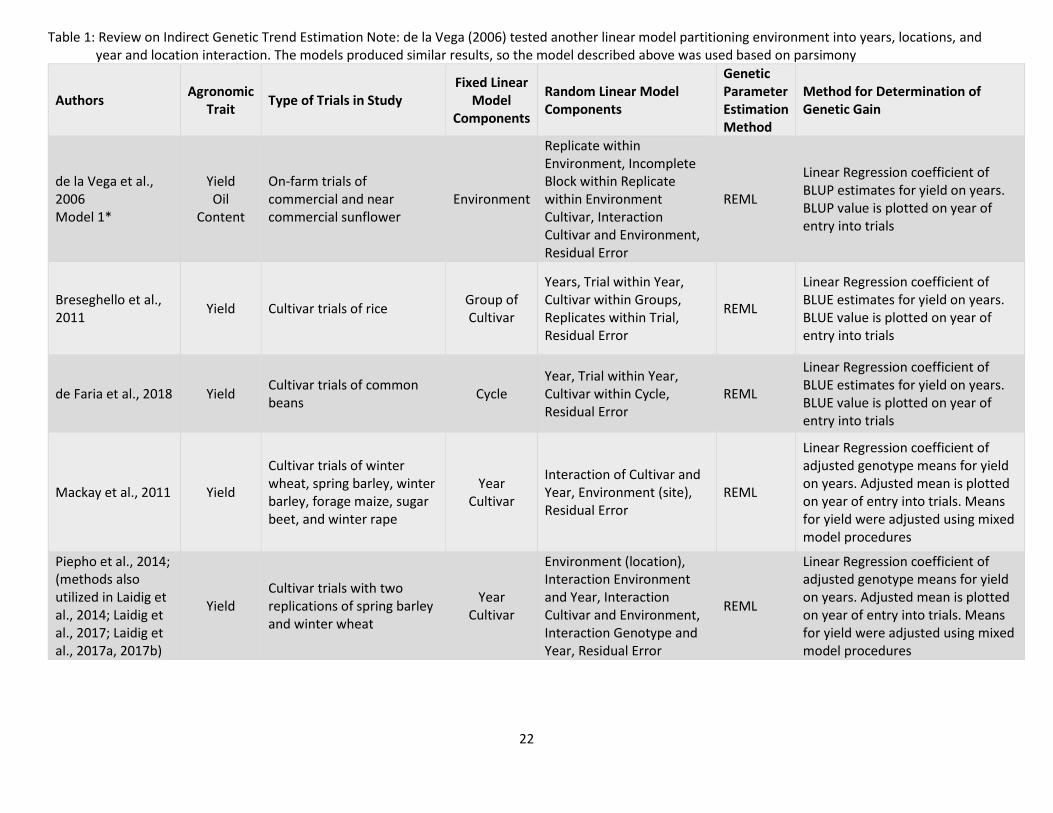
Table 1: Review on Indirect Genetic Trend Estimation Note: de la Vega (2006) tested another linear model partitioning environment into years, locations, and year and location interaction. The models produced similar results, so the model described above was used based on parsimony

Authors Agronomic

Trait Type of Trials in Study

Fixed Linear Model

Components

Random Linear Model Components

Genetic Parameter Estimation Method

Method for Determination of Genetic Gain

de la Vega et al., 2006 Model 1*

Yield Oil

Content

On-farm trials of commercial and near commercial sunflower

Environment

Replicate within Environment, Incomplete Block within Replicate within Environment Cultivar, Interaction Cultivar and Environment, Residual Error

REML

Linear Regression coefficient of BLUP estimates for yield on years. BLUP value is plotted on year of entry into trials

Breseghello et al., 2011

Yield Cultivar trials of rice Group of Cultivar

Years, Trial within Year, Cultivar within Groups, Replicates within Trial, Residual Error

REML

Linear Regression coefficient of BLUE estimates for yield on years. BLUE value is plotted on year of entry into trials

de Faria et al., 2018 Yield Cultivar trials of common beans

Cycle Year, Trial within Year, Cultivar within Cycle, Residual Error

REML

Linear Regression coefficient of BLUE estimates for yield on years. BLUE value is plotted on year of entry into trials

Mackay et al., 2011 Yield

Cultivar trials of winter wheat, spring barley, winter barley, forage maize, sugar beet, and winter rape

Year Cultivar

Interaction of Cultivar and Year, Environment (site), Residual Error

REML

Linear Regression coefficient of adjusted genotype means for yield on years. Adjusted mean is plotted on year of entry into trials. Means for yield were adjusted using mixed model procedures

Piepho et al., 2014; (methods also utilized in Laidig et al., 2014; Laidig et al., 2017; Laidig et al., 2017a, 2017b)

Yield Cultivar trials with two replications of spring barley and winter wheat

Year Cultivar

Environment (location), Interaction Environment and Year, Interaction Cultivar and Environment, Interaction Genotype and Year, Residual Error

REML

Linear Regression coefficient of adjusted genotype means for yield on years. Adjusted mean is plotted on year of entry into trials. Means for yield were adjusted using mixed model procedures

23

Mackay et al. (2011) found when year and genetic effect were modeled as random effects,

variability in one factor could be allocated to the other leading to bias in the estimates. This bias does

not happen when these effects are modeled as fixed effects. In order to assess trends, Piepho et al.

(2014) conducted regressions of adjusted year means plotted against time to assess non-genetic trends,

and genotype means plotted against year when a cultivar (genotype) entered the trial to assess genetic

trends.

Potential for On-farm Estimation of Genetic Trends

Factorial complete block approaches to evaluate genetic trends would require crop producers to

have specialized equipment in order to plant small plots of historical varieties or plant historical varieties

with less desirable agronomic qualities on a large scale throughout their production operation. In

addition, crop producers would need to maintain and conduct seed increases of these historical

varieties. The time and labor involved with factorial complete block approaches make them impractical

in crop production operations. Thus, this approach is not practical for on-farm estimation of genetic

trends.

Crop producers, in general, do not have the ability to conduct research with small plots, in

replicated trials with equipment used to farm large tracts of land. In addition, the numbers of cultivars

grown on a farm and the length of time the cultivars are grown limit the amount of data that can be

gathered from a farm on an annual basis. Table 2 outlines information on cultivar selection criteria,

number of varieties grown on-farm per year, and the length of time a cultivar is utilized on-farm. Maize,

soybeans, and wheat are included in the table since these crops are consistently grown on a yearly basis

of crop producers in North Dakota (J. Messer, personal communication, January 17, 2020; B. Peterson,

personal communication, January 17, 2020). Practical Farmers of Iowa (PFI) have demonstrated it is

possible to conduct on-farm research using best practices for experimental designs and data analyses

without significant impacts on farm income (Farmer-Led Research, n.d.). Indeed, some research

24

treatments have had such a large positive impact on income that some farmers have converted their

entire operations before the agreed upon timelines for multi-year experiments. Administrative staff for

PFI aid producers who wish to design and conduct on-farm directed projects. Assistance occurs in areas

of record-keeping, demonstration and design of on-farm experiments that follow best practices to

assure data analyses will answer the research questions and can be used to make decisions. On-farm

research is also conducted by Discovery Farms in the states of Arkansas, Minnesota, North Dakota,

Washington, and Wisconsin. Discovery Farms on-farm research generally focuses on environmental

impacts of production agriculture and partners with local producers, agriculture extension services,

United States Geological Survey, conservation districts, and other local agencies. (Discovery Farm

Program | Arkansas Agricultural Experiment Station, n.d.; Discovery Farms Minnesota, n.d.; Discovery

Farms Washington, n.d.; Discovery Farms Wisconsin, n.d.; North Dakota Discovery Farms, n.d.). While

the Discovery Farm on-farm research program may not offer the versatility of choosing a research topic

like PFI does, it is an opportunity for producers who participate to learn about best practices for

experimental design and to become involved with organizations that can assist with the design and

implementation of on-farm research.

Table 2: Summary of Cultivar Criteria in North Dakota (J. Messer, personal communication, January 17, 2020; B. Peterson, personal communication, January 17, 2020)

Soybean Maize Hard Red Spring Wheat

Common Criteria for Selection

Yield, disease resistance, plant structure

Yield, performance on specified soil type, plant structure, stress tolerance

Yield, disease resistance, protein, standability, performance on specified soil type

Cultivars Grown per Farm per Year

2-3 cultivars 2-8 cultivars 2-3 cultivars

Length of Farm Utilization for Cultivars

2-3 years 2-5 years 3-6 years

The use of connected incomplete block designs should be possible to implement by crop

producers. Crop producers would record the yield of treatments of any size fitting the routine

25

operations of the farm. Field trial data can then be adjusted to a standard unit such as pounds per acre

or kilograms per hectare. The field yield records should be taken from the weight of harvested material

on a certified scale or calibrated grain cart scale due to errors associated with the indirect measurement

of yield from yield monitoring systems. This type of collection of data is typical of crop producer

operations at harvest. Within replications of the same treatment producers should not utilize variable

rate seeding or fertilizer applications. Additional information to include with yields will include year and

the field identification (environment). Breseghello et al. (2011) notes for the estimation of genetic trend,

common cultivars are needed to connect non-genetic information from consecutive years to allow for

the control of the environmental variation. Mackay et al. (2011) limited data included in his genetic

trend analysis to varieties grown three or more seasons. This criterion of cultivars grown for three or

more seasons is met by Piepho et al. (2014), Laidig et al. (2014), Laidig et al (2017), Laidig et al. (2017a,

2017b). This criterion could also be met with data taken by crop producers. Table 2 shows for crops

commonly occurring in rotations, multiple cultivars are grown on a farm and these are grown across

multiple years. If cultivars are added and dropped from a crop production operation but are connected

across years, data will allow for the control of environmental variation. The model and a discussion of

the methodologies from Table 1 separating genetic variation from non-genetic effects on-farm can be

found in Appendix F.

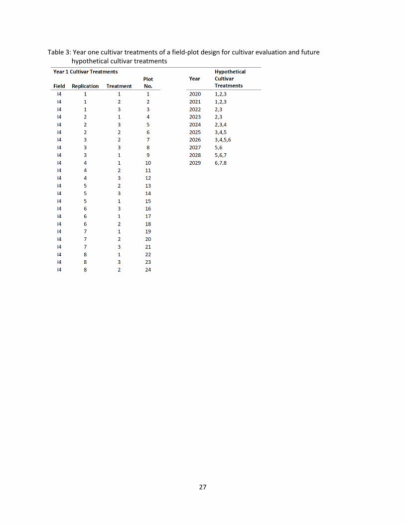
Table 3 and Figure 2 are an example of a design a producer could use on-farm to evaluate

genetic trends. Table 3 shows the replications, treatments, and assigned plot number for the first year of

data used genetic trend estimation. Table 3 also shows how the cultivars grown by the producer may

possibly change over the next 10 years. Each cultivar treatment number represents a different cultivar

being utilized in farm production. Numbers of cultivars in the hypothetical 10-year table are consistent

with crop production practices in North Dakota (see Table 2). The proposed design for each individual

year utilizes randomized complete block design (RCBD; see Appendix E). However, looking at all the

26

blocks from all the years used in the genetic trend analysis, cultivars are added and dropped creating

connected incomplete blocks if cultivars over years. Figure 2 shows an aerial photo of field-plots at the

USDA-ARS Area 4 Soil Conservation Districts Cooperative Research Farm and a possible plot design

within these plots based on information from Table 3. The size of the plots and distance between plots is

proposed in increments of 30 feet to accommodate planter and combine header width. Plot size can be

adjusted to fit on-farm equipment. Geographic information systems (GIS) programs may be used with

data gathered on-farm to create application maps for variable rate equipment to allow producers easier

planting and application of inputs to on-farm research plots. Figure 3 shows examples of maps created

in this manner (J. Messer, personal communication, January 17, 2020). Table 4 and Figure 4 are an

example of a design a producer could use on-farm to evaluate genetic trends utilizing information from

field variability that does not create a uniform field pattern. The field design shown in Figure 4 utilizes

information from satellite imagery of crops and soil variability measures to zone the field into more

uniform blocks (M. Liebig, personal communication, March 24, 2020). Many crop producers currently

have fields broken into management zones based on variability (J. Messer, personal communication,

January 17, 2020; B. Peterson, personal communication, January 17, 2020). If producers have

management zones created for fields, blocks may be fit in non-uniform shapes.

27

Table 3: Year one cultivar treatments of a field-plot design for cultivar evaluation and future hypothetical cultivar treatments

28

Figure 2. Field-plot design for cultivar evaluation. Field picture, basic information, and blocking structure based on work of the USDA-ARS Area 4 Soil Conservation District Cooperative Research Farm. From Liebig, M. (2020, March 23). Personal communication. Reprinted with permission

29

Elevation Map Electrical Conductivity Map Aggregated Data Map

Figure 3. GIS Mapping of Field Variability in Washburn North Dakota. From Messer, J. (2020, January 17). Personal communication. Reprinted with permission Table 4: Year one cultivar treatments of a field-plot design for cultivar evaluation maximizing uniformity

and future hypothetical cultivar treatments

30

Figure 4. Field-plot design for cultivar evaluation maximizing uniformity. Field information and blocking structure based on field variation from the USDA- ARS Area 4 Soil Conservation District Cooperative Research Farm. From Liebig, M. (2020, March 23). Personal communication. Reprinted with permission

SUMMARY

The first portion of this paper examined basic genetic principles of genetic gain and

methodology of estimating genetic gain. Prediction of genetic gain from one generation to the next

utilizes linear models that allow phenotype variance to be broken down into components (Equation 5

and 6). Within the genetic component of phenotype, only the additive effect of alleles is inherited. This

is a genotype’s breeding value. Estimates of genetic gain or response to selection (R) over a cycle of

breeding can be found if narrow sense heritability (h2) and selection differential (S) or standard

deviation of the phenotype (σph) and intensity (i) of selection are known or estimated (Equation 11 and

31

13). Heritability and estimations of variance components within models can be estimated using multiple

methodologies including ANOVA, simple linear regression, and REML combined with Henderson’s mixed

model (see Appendix B, C, and D).

The second portion of this paper considered the feasibility of estimating genetic trend on-farm.

Two approaches have been used to estimate genetic trends. These approaches involve either a balanced

set of genotypes and management practices applied to each of several fields across multiple years,

where fields represent complete blocks, or an unbalanced set in which fields and years are connected by

a subset of genotypes and management practices, where each field represents a type of incomplete

connected block (Eccleston & Hedayat, 1974). Based on review of genetic trend estimation methods,

factorial complete block designs (Duvick, 1997, 2005) are not feasible for on-farm use while connected

incomplete block designs (Table 1) have existing procedures which can be applied from trial data to on-

farm data in order to evaluate genetic trends. These methods of genetic trend estimation do not require

large investments of resources or time and can be incorporated into current production practices. The

management practices common to many farms of growing multiple varieties of a crop each year and

growing that cultivar for multiple years paired with best practices for experimental design allow for the

control of environmental and yearly variation within on-farm data. By estimating the genetic trend on-

farm, crop producers would have a powerful tool enabling them to see how much of their agronomic

trait, such as yield, is coming from genetics. This would aid in the selection of varieties and provide an

independent assessment of genetic effect.

Many crop producers within the State of North Dakota have not been exposed to genetic or

statistical concepts needed to understand genetic gain and its estimation. In order to see value in

genetic trend estimates of genetic gain, crop producers should understand these principles. This paper

presents some of these basic principles. The first important concept that should be communicated is the

difference between qualitative and quantitative traits. The second important idea is that if a plant

32

breeder is improving quantitative traits, the breeder must understand the variance of individuals or

groups in order to select for this variation. If breeders select for variation within a population, the crop

producer must understand the components contributing to variance; genetic, environment, and

interaction effects. Breeders improve crops through the genetic portion. Crop producers should

understand when selecting for variations within the genetic portion not all the components of genetic

variance are transferred to the offspring. Crop producers should have a basic understanding of the

components of genetic variance: additive, genetic, and epistatic effects. Of these three components,

only additive genetic effects are transferred to offspring. The genetic gain from breeding programs is

dependent on selection of the additive genetic components since this is all that is inherited by offspring

from the components of the genotype. Methods exist to estimate and measure how much of the

genotypic variance is due to additive genetic variance and to estimate genetic gain from selection. Once

genetic gain is understood, the amount of realized genetic gain from genetic trend estimations informs a

crop producer how much of the increase in an agronomic trait, such as yield, is due to the genetics of

the crop and not just the environment and management practices. By understanding this concept, price

changes with improved varieties may be analyzed independently on-farm to find if the expected

agronomic trait increase is worth the price.

Lack of crop producer exposure to genetic concepts is one communication challenge that faces

plant breeder and crop producer interactions. Lack of funding to university extension programs has

resulted in loss of information from unbiased evaluations of cultivar performance. Funding cuts to

universities also affect public sector plant breeding programs. When surveying public sector plant

breeders, Shelton and Tracy (2017) found that most plant breeders see support of stakeholder

commodity groups as a necessary requirement for continuance of public breeding positions upon their

retirement. Communication between crop producers (stakeholders) and public sector plant breeders is

necessary to ensure continued support of breeding programs and the development of cultivars

33

especially in crops, geographic locations, and management systems that are not profitable enough for

private industry (Shelton & Tracy, 2017).

Perhaps the greatest challenge is effective communication of plant breeding and statistical

concepts to crop producers. This is due in part to limited interactions that build trust between crop

producers and plant breeding educators. A difficult task for professionals and educators in any

agriculture discipline, including plant breeding, is to become familiar with the day to day operations and

needs of producers within their geographic region. This is especially difficult if educators and consultant

professionals are not from the region in which they work. Agriculture differs greatly across regions.

None-the-less, crop producers in every region use language that expresses their experience with land

and its value in terms of production costs and gross receipts from sale of their products. Plant breeding

educators need to first listen and learn the language that is relevant to crop producers.

The creation of support networks between crop producers and plant breeding educators allows

for effective communication. These networks are created through interaction, the learning of a

common language, and the building of trust. Interaction occurs during post-secondary education,

professional development events, and interpersonal interaction. Many crop producers do not interact

with plant breeding educators during post-secondary education. This lack of post-secondary education

interaction results in professional development events being the first-time interaction occurs between

crop producers and plant breeding educators. Crop producers attend professional development events

that involve many subject areas. Attendance of many professional development events across a wide

array of subject areas by plant breeding educators allows for many interaction opportunities with crop

producers. Furthermore, attendance of professional development events across a wide array of subject

areas allow exposure to common language used by crop producers. Once a common language is

developed, trust is built from these continued interactions. The building of trusted support networks

leads to interactions of crop producers and plant breeding educators on interpersonal levels such as

34

visits to farms or breeding facilities. The establishment of a common language and trust allows mutually

beneficial relationships to be created between crop producers and plant breeding educators. These

relationships allow support from crop producers for continuation of plant breeding programs and the

development of cultivars that best serve crop producers.

35

Appendix A: Quantitative Plant Breeding Basics

The goal of plant breeding is the genetic improvement of plants. A plant trait, such as yield or

disease resistance, is selected for improvement. This trait has a genetic component termed the

genotype. The phenotype is influenced by the genotype, environment, and how the genotype and

environment interact. The environment includes differing climatic conditions, different cultural

production and management practices, and differing types of abiotic and biotic stressors. Variation

exists among cultivars due to genotype, environment, and genotype and environmental interaction. The

genetic portion of this variation is what causes selectable differences and what the plant breeder uses

for selection. The genotypic component of a trait may be qualitative or quantitative. A qualitative trait

variation among genotypes is not continuous and can be separated into discrete classes. This is what

many of us remember from high school with Gregor Mendel’s pea plants – flowers are either purple or

white; there is no value in between. This type of trait is usually controlled by one or a small number of

major genes. With a quantitative trait, variation is continuous and cannot be separated into discrete

classes. Examples include most agronomic traits of economic value such as yield per unit land,

physiological maturity, or response to planting densities. In general, many alleles and multiple loci

influence these traits. The locations of the alleles and loci within the genome are mostly unknown, and

the effects of individual alleles and their interactions are the subject of discovery research, but are

mostly unknown (Bernardo, 2020). Many agronomic traits breeders seek to improve are quantitative

traits and as such statistics is a major subject area used for the evaluation, identification, and selection

of superior genotypes for the use in breeding programs.

A challenge in breeding projects is to select genetically superior genotypes to release for

commercial crop production or to use as parents in the production offspring. How does a breeder select

the best genotype for any given trait if the trait values are due to valuable alleles distributed among

hundreds of loci? What if the genes interact with each other, aka epistasis, to produce different

36

characteristics? What if the environment interacts with the genes and changes the phenotype?

Statistical methods help breeders with this selection process and to account for these questions by

allowing them to estimate the components of variability of the plants within the breeding program and

select genetically superior genotypes.

When evaluating genotypes to use for crossing in a breeding program or for release into

commercial crop production, plant breeders generally record a great deal of data. In plant breeding

often genotypes are grown in multiple plots that contain replicated genotypes. Development of

replicable genotypes enables the breeder to determine what proportion of the variability among plots

can be repeatedly attributed to genotypes, also known as heritable, and what part of the variability is

due to non-genetic sources. In addition, the climatic conditions of field sites are recorded. The pedigree

of the replicable genotypes may also be known.

In order to select superior genotypes, plant breeders utilize mathematical models and fit the

models to the data. This mathematical model is generally an equation or set of equations that describe,

represent, or approximate the physical, chemical, or biological (genetic) states of the evaluated entities

(Motulsky, 2014). The equations in the model define a dependent variable or outcome that is the result

of one or more independent variables. The independent variables represent the parameters of the

model. Once the model is fit to the data, estimates and predictions of the influence of the independent

variables, can be calculated. In addition, the confidence in these estimates and predictions can be

calculated.

Appendix B: ANOVA

ANOVA is a procedure used to analyze differences among the means of groups. The ANOVA

evaluates if the means of two or more groups are more different than the unexplained variability

associated with measuring values of members belonging to each group. ANOVA is based on a null

37

hypothesis. The null hypothesis is generally all groups share the same mean, and the alternative is all

populations do not share the same means. ANOVA works by partitioning the sum of squared deviations

for each source of variability represented by the parameters of the model. Assumptions of ANOVA

include samples are randomly selected and representative of the population, observations in each

sample are independent, the deviations from the model are normally distributed, and identical across all

sources of variability (Motulsky, 2014). ANOVA calculations are affected by the type of effects ascribed

to the model parameters. Type 1 ANOVA analyzes models consisting of parameters considered to be

fixed effects. Fixed effects represent groups for which the differences between groups is of interest only

to this experiment. There is no intention of using the results of the experiment to infer outcomes in any

other experiment or under any other conditions. From a technical perspective fixed effects do not have

a covariance that needs to be estimated. Type II ANOVA analyzes models with random effect

parameters. Random effects assume the sources of variability represented by the parameters in the

model are from a sample of the population. The purpose is to draw inferences from the experiment to a

larger population from which the samples were drawn. Groups are randomly selected from all possible

groups and the results of the ANOVA indicate whether there are differences among the groups, and that

these differences indicate not only are the differences in among the sample of groups, but also among

all groups in the population of groups. Estimates of the random effects require an estimate of

covariance among members. Because estimates of covariance are biased with small sample sizes, say

less than 30, the estimates of random effects should be based on a large sample size. Covariance refers

to the measure of the joint variability of two random variables. An example of covariance is Galton’s

comparison of measured heights between parent and offspring. One parent contributes half of its

genetic composition to its offspring which causes a covariance between the parent and offspring

(Bernardo, 2020). Models that include fixed and random effects are referred to as mixed models. Type III

ANOVA allows for the analysis of models with both fixed and random effects. Table 5 shows possible

38

values of variance components calculated from an ANOVA. These components are calculated by setting

the expected mean square formula equal to the mean square value calculated by ANOVA and solving for

the known variance component (Fehr, 1991). An example of variance components estimated from

ANOVA can be utilized to calculate heritability can be found in Table 6.

Table 5: Example ANOVA table output from R program using data from Agronomy 528 (Beavis, 2018). Where σe

2 is the variance of the residual error, σG2 is the genotypic variance, and σE

2 is the environmental variance, σGE

2 is the variance of the interaction of genetics and environment, r is the number of replications 2 in this data set, and t is the number of environments 10 in this data set. Linear Model: Yij = µ +

Gi + Ej + GEij + eij

Where : Where Y is the measured phenotype (yield) of the i genotype grown in the j environment, µ is the overall mean of the sample, G is the effect of the i genotype on the individual (random effect), E is the effect of the j environment on the individual (fixed effect), GE is the interaction between the i genotype and the j environment (random effect), and the and e is the residual error or residual effects associated with the i genotype and j environment Analysis of Variance: Type III ANOVA

Source Df Sum

Squares Mean

Square Expected Mean

Square Calculated variance components based

on Expected Mean Squares

env 9 384708 42745

line 49 131139 2676 σe2 + rσGE

2 + rt σG2 σG

2 =111.7

env: line 441 194911 442 σe2 + rσGE

2 σGE2 =148

Residuals 500 72949 146 σe2 σe

2 =146

Table 6: Equations for Calculating Heritability by the Variance Component Method based on Fehr, 1991

Selection Method Equation

Single-Plant basis with plants of population not divided into plots or blocks

h2=

σG2

_______________ σw

2 + σ2 + σGE2 + σG

2

Single-Plant basis with plants of population divided into plots or blocks

h2=

σG2

_______________ σw

2 + σGE2 + σG

2

Plot basis

h2=

σG2

_______________ σe

2 + σGE2 + σG

2

Entry-Mean basis

h2=

σG2

_______________ σe

2/rt + σGE2/t + σG

2

Where: h2 is narrow sense heritability, σG2 is the genotypic variance, σw

2 is the variance among plants within a plot, σ2 variance among plots or blocks, σe

2 is the variance of the residual error, σGE

2 is the variance of the interaction of genetics and environment, r is the number of replications, and t is the number of environments

39

Appendix C: Linear Regression to Estimate Heritability

Lush outlined methods for measuring heritability based on his breeder’s equation. His most useful

approach is the linear regression of parents to their offspring used for estimating individual values for

narrow sense heritability (Lush, 1940, 1994). The linear regression model is:

Yi = a + bXi + e (Equation 14; Fehr, 1991)

Where Yi is the performance of offspring of the ith parent, a is the mean performance of all parents, b is

the linear regression coefficient, Xi is the performance of the ith parent, and ei is the residual error

associated with the measurement of Xi

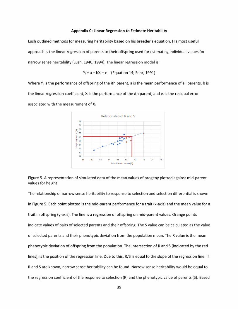
Figure 5. A representation of simulated data of the mean values of progeny plotted against mid-parent values for height The relationship of narrow sense heritability to response to selection and selection differential is shown

in Figure 5. Each point plotted is the mid-parent performance for a trait (x-axis) and the mean value for a

trait in offspring (y-axis). The line is a regression of offspring on mid-parent values. Orange points

indicate values of pairs of selected parents and their offspring. The S value can be calculated as the value

of selected parents and their phenotypic deviation from the population mean. The R value is the mean

phenotypic deviation of offspring from the population. The intersection of R and S (indicated by the red

lines), is the position of the regression line. Due to this, R/S is equal to the slope of the regression line. If

R and S are known, narrow sense heritability can be found. Narrow sense heritability would be equal to

the regression coefficient of the response to selection (R) and the phenotypic value of parents (S). Based

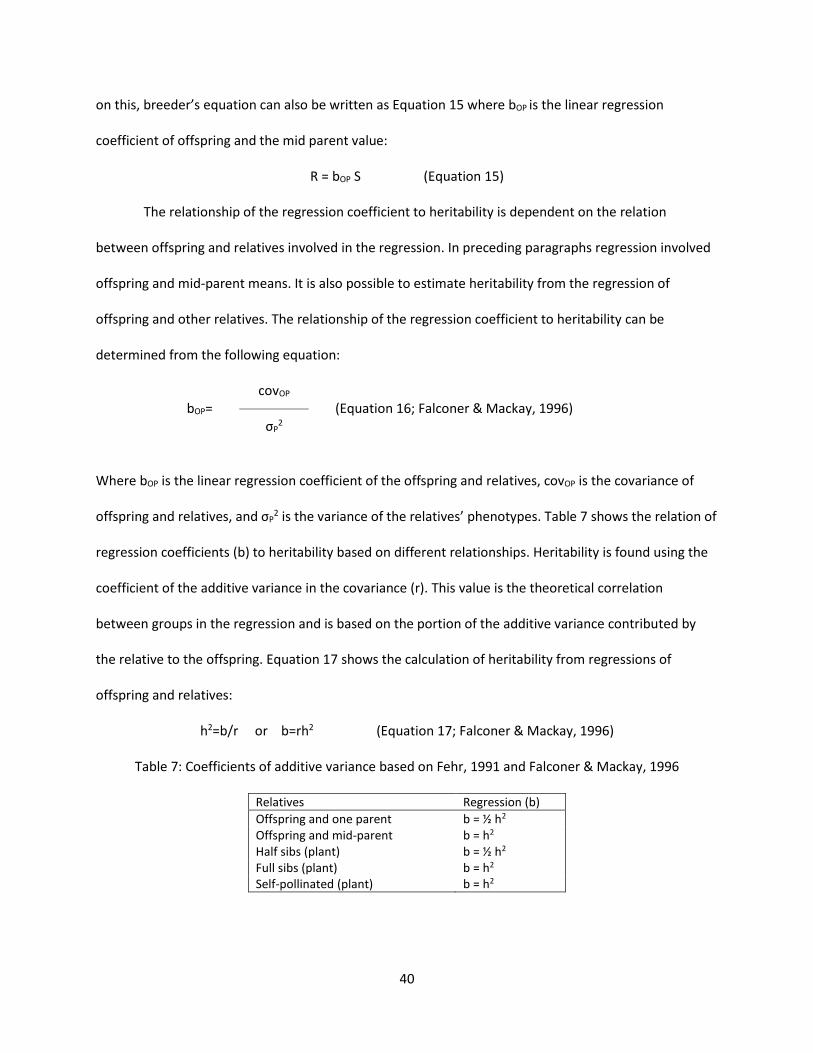
40

on this, breeder’s equation can also be written as Equation 15 where bOP is the linear regression

coefficient of offspring and the mid parent value:

R = bOP S (Equation 15)

The relationship of the regression coefficient to heritability is dependent on the relation

between offspring and relatives involved in the regression. In preceding paragraphs regression involved

offspring and mid-parent means. It is also possible to estimate heritability from the regression of

offspring and other relatives. The relationship of the regression coefficient to heritability can be

determined from the following equation:

bOP=

covOP _______________

σP2

(Equation 16; Falconer & Mackay, 1996)

Where bOP is the linear regression coefficient of the offspring and relatives, covOP is the covariance of

offspring and relatives, and σP2 is the variance of the relatives’ phenotypes. Table 7 shows the relation of

regression coefficients (b) to heritability based on different relationships. Heritability is found using the

coefficient of the additive variance in the covariance (r). This value is the theoretical correlation

between groups in the regression and is based on the portion of the additive variance contributed by

the relative to the offspring. Equation 17 shows the calculation of heritability from regressions of

offspring and relatives:

h2=b/r or b=rh2 (Equation 17; Falconer & Mackay, 1996)

Table 7: Coefficients of additive variance based on Fehr, 1991 and Falconer & Mackay, 1996

Relatives Regression (b)

Offspring and one parent b = ½ h2 Offspring and mid-parent b = h2 Half sibs (plant) b = ½ h2 Full sibs (plant) b = h2 Self-pollinated (plant) b = h2

41

The use of linear regression of offspring to parents is based on assumptions of diploid

inheritance; random-mating parental generation before selection; population is joint equilibrium;

parents are not inbred; and no environmental correlation between the performance of parents and

offspring (Fehr, 1991). However, most breeding individuals are selected to mate, and these individuals

are controlled in the way they mate such as inbreeding or crossbreeding. Falconer & Mackay (1996)

note assortative mating, which is the selection of parents before mating, has little effect on mid-parent

regression.

Appendix D: Mixed Models

In his 1975 paper Best Linear Unbiased Estimation and Prediction Under a Selection Model,

Henderson outlined the linear mixed model for application in genetics in matrix form as:

y = XB + Zu + e (Equation 18)

Where y, B, u, and e are vectors of data (measurements on all individuals). The value y is the vector

corresponding to phenotype, B is the vector of fixed effects to be estimated such as environment or

year, u is the vector of random effects to be estimated such as individual genotypic values, and e is the

vector of random error (random effect). X is a matrix of fixed effects; Z is a matrix of random effects.

The variances (var) and means (E) of the random effects and phenotype vector (y) of the model are

given below and assume the data is normally and independently distributed:

var(y) = ZGZ’ + R = V, var(u) = G, var(e) = R

E(u) = E(e) = 0, E(y) = XB

The matrix model of Equation 18 can also be written as a scalar notation. The example below will utilize

the scalar model from equation 5 and denote it in matrix form:

Yij = µ + Gi + Ej + eij (Equation 5)

This matrix model using the parameter distinctions as Equation 5:

42

y = XE + ZG + e (Equation 19)

In equation 19 environments are fixed effects and the genotypes are random effects. The critical

assumption of mixed models and calculations involving them is the distribution from which the data is

sampled is assumed normal with a variance (Hill, 2014).

Applications of this model in Henderson’s work include estimating the linear function of B

(termed Best Linear Unbiased Estimator or BLUE), testing hypothesizes regarding B, predicting u or a

linear function of u (termed Best Linear Unbiased Prediction or BLUP), and predicting linear function of B

and u jointly. Another application is the estimation of genetic variances and covariances G, R, and/or the

total variance and adjusting the data for fixed effects (Henderson, 1975; Thompson, 2008). In

Henderson’s model, the calculations used to fit the linear model to the data handle unbalanced designs,

are able to use information for all relatives measured to improve estimates, use all recorded information

available in optimum way, allow for missing data, and can take account of selection and nonrandom

mating provided all the data on which the decisions were taken are included. In addition, it can be

incorporated into likelihood methods used to estimate quantitative genetic parameters for estimation

of variance components (Hill & Kirkpatrick, 2010; Bernardo, 2020).

Bernardo (2020, p. 228 -260) provides a detailed breakdown of matrix algebra, how BLUP’s

adjust values with a shrinkage term, calculation of BLUP’s for inbreds and clones, calculations for BLUP’s

and single crosses, and calculations for BLUP’s for untested inbreds and clones.

Appendix E: Experimental Practices and Field-Plot Design

Randomization applies treatments, such as a cultivar being evaluated within a genetic trend

experiment, at random to several experimental units (Clewer & Scarisbrick, 2001). A treatment on-farm

may be a strip of a cultivar the width of at least one combine pass and extend the length of the field

(“Research Protocols, n.d.). Experimental units, often referred to as plots in plant breeding field trials,

43

are assigned treatments at random. Randomization allows for the creation of homogeneous treatment

groups through the elimination of biases or judgments from the individuals conducting the experiment.

Every treatment will have an equal chance of being assigned to any experimental unit. For example,

individuals using randomization will be unable to bias an experiment by placing all treatments of a

genotype thought to be superior on the most fertile land within a field. Experimental units also must be

replicated. Replication is the application of each treatment to multiple experimental units. Replication

allows the estimation of experimental error to measure the variation in the response of treatments or

other uncontrolled experimental factors (Clewer & Scarisbrick, 2001). In the example of a genetic trend

experiment, replication allows the separation of whether variation between cultivars is due to genetic

effects or to non-genetic variation. Replication also increases the precision of an experiment. In a

genetic trend experiment, replications may be accomplished within one season by growing multiple

experimental units of every treatment. These units may be at the same or multiple locations.

Replications may also occur over multiple years.

The field-plot technique of blocking allows for the reduction in experimental error and the

increase in precision of the experiment by growing treatments under more uniform conditions.

Replicated experiments used to evaluate genotypes in plant breeding primarily use randomized

complete block design (RCBD) or incomplete block design (Fehr, 1991). A complete block contains all

treatments being evaluated. Each treatment occurs once within each block. This allows the treatments

to be compared within blocks. Variation between blocks does not affect comparisons of the treatments.

Due to each treatment occurring within every block, blocks and replications are equivalent. Blocking

advantages include reduction of experimental error by allowing blocking that accounts for site

variability, such as topography or soil fertility factors. Blocking also allows for the separation of non-

genetic factors that deal with agronomic production practices. For example, a block can be planted or

harvested at one time, if a precipitation event occurs preventing the harvesting of other blocks, the

44

statistical analysis of the block design will allow for separation of treatment effects, such as genetic

effects, from the non-genetic effects caused by the precipitation event. Each block must be planted,

treated, and harvested at the same time to ensure the precision of treatment comparisons. Blocking

allows for the use of several sites if the site variability does not impose interaction between blocks and

treatments (Clewer & Scarisbrick, 2001). Knowledge of the variation at field sites is required to conduct

randomized complete block design. Blocks must be positioned correctly to ensure uniformity of non-

genetic factors throughout the block. Figure 4 shows a blocking pattern design from the USDA-ARS Area

4 Soil Conservation District Cooperative Research Farm. Satellite imagery of crops and soil variability

information throughout the field were used to create uniform zones within this field (M. Liebig, personal

communication, March 24, 2020). Complete blocking does not allow the division of replications into

smaller units. The disadvantage of complete blockings is the inability to adjust the performance of

treatments for non-genetic variation within replications (Fehr, 1991). In addition, if there are missing

values within a block, the statistical analysis may have difficulty separating the effects of the block and

treatment (Clewer & Scarisbrick, 2001). Missing data may result from environmental factors, abiotic

disease, biotic disease, or poor data management. Figure 6 outlines an example of a randomized

complete block design (G. Enders, personal communication, March 12, 2020).

Incomplete block designs do not contain all treatments within a block. Incomplete block designs

provide more control over environmental variation within a replication than with complete block design

since a replication does not need to contain all treatments. Blocks do not have to be large enough to

accommodate all treatments. As the amount of treatments increase, so does the area required to

include all treatments within a block. As the area of a block increases in size, it becomes more difficult to

maintain the uniformity throughout the block. Incomplete block designs allow for smaller, more uniform

blocks that may not contain all treatments. Incomplete block designs allow for the adjustment of

performance of each treatment according to the productivity of the plots in which it is evaluated. If one

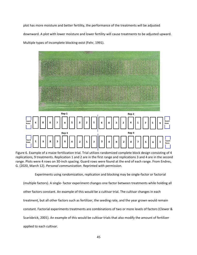
45

plot has more moisture and better fertility, the performance of the treatments will be adjusted

downward. A plot with lower moisture and lower fertility will cause treatments to be adjusted upward.

Multiple types of incomplete blocking exist (Fehr, 1991).

Figure 6. Example of a maize fertilization trial. Trial utilizes randomized complete block design consisting of 4 replications, 9 treatments. Replication 1 and 2 are in the first range and replications 3 and 4 are in the second range. Plots were 4 rows on 30-inch spacing. Guard rows were found at the end of each range. From Endres, G. (2020, March 12). Personal communication. Reprinted with permission.

Experiments using randomization, replication and blocking may be single-factor or factorial

(multiple factors). A single- factor experiment changes one factor between treatments while holding all

other factors constant. An example of this would be a cultivar trial. The cultivar changes in each

treatment, but all other factors such as fertilizer, the seeding rate, and the year grown would remain

constant. Factorial experiments treatments are combinations of two or more levels of factors (Clewer &

Scarisbrick, 2001). An example of this would be cultivar trials that also modify the amount of fertilizer

applied to each cultivar.

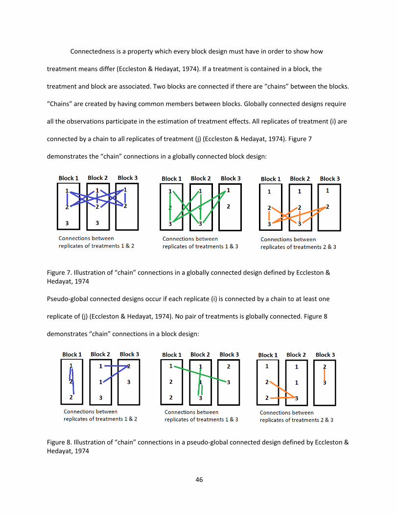
46

Connectedness is a property which every block design must have in order to show how

treatment means differ (Eccleston & Hedayat, 1974). If a treatment is contained in a block, the

treatment and block are associated. Two blocks are connected if there are “chains” between the blocks.

“Chains” are created by having common members between blocks. Globally connected designs require

all the observations participate in the estimation of treatment effects. All replicates of treatment (i) are

connected by a chain to all replicates of treatment (j) (Eccleston & Hedayat, 1974). Figure 7

demonstrates the “chain” connections in a globally connected block design:

Figure 7. Illustration of “chain” connections in a globally connected design defined by Eccleston & Hedayat, 1974 Pseudo-global connected designs occur if each replicate (i) is connected by a chain to at least one

replicate of (j) (Eccleston & Hedayat, 1974). No pair of treatments is globally connected. Figure 8

demonstrates “chain” connections in a block design:

Figure 8. Illustration of “chain” connections in a pseudo-global connected design defined by Eccleston & Hedayat, 1974

47

Appendix F: Model for On-Farm Genetic Trend Estimation

Appendix F includes regression equations and a proposed linear mixed model for on-farm

genetic trend analysis as well as procedures to adjust cultivar values within the genetic trend analysis

using REML, BLUE, and BLUP procedures. Equations 20 and 21 outline the regression model.

Gi = 𝛽ri + Hi (Equation 20; Piepho, 2014)

Where Gi is the effect of the i genotype, ri is the year the genotype i entered field trials, 𝛽 is a fixed

regression coefficient for genetic trend, and Hi models random deviation from the genetic trend line.

Assumptions made are that the random effects are distributed as a normal random variable with zero

mean and a variance of σH2.

Yk = 𝛾tk +Zk (Equation 21; Piepho, 2014)

Where Yk is the effect of the k year, tk is the year the genotype k entered cultivar field trials, 𝛾 is a fixed

regression coefficient for non-genetic trend, and Zk models random deviation from the non-genetic

trend line. Assumptions made are that Zk follows a normal distribution with zero mean and a variance of

σz2.

The proposed method for estimation of genetic trend on-farm will use a linear mixed model.

The scalar model is given by Equation 22:

Yijk = µ + Gi + Ej + Ak + GEij + GAik + eijk (Equation 22)

Where Y is the measured phenotype with i genotype, grown in the j field in the k year, µ is the overall

mean of all genotypes environments and years, G is the fixed effect of the i genotype, E is the random

effect of the j field, A is the random effect of the k year on the individual, GE is the random effect of

interaction of the i genotype with the j field, GA is the random effect of the interaction of the i genotype

with the k year on the individual, and e is the residual error associated with the i genotype, j field, and k

year. This model assumes that genetic trends are to be determined per year.

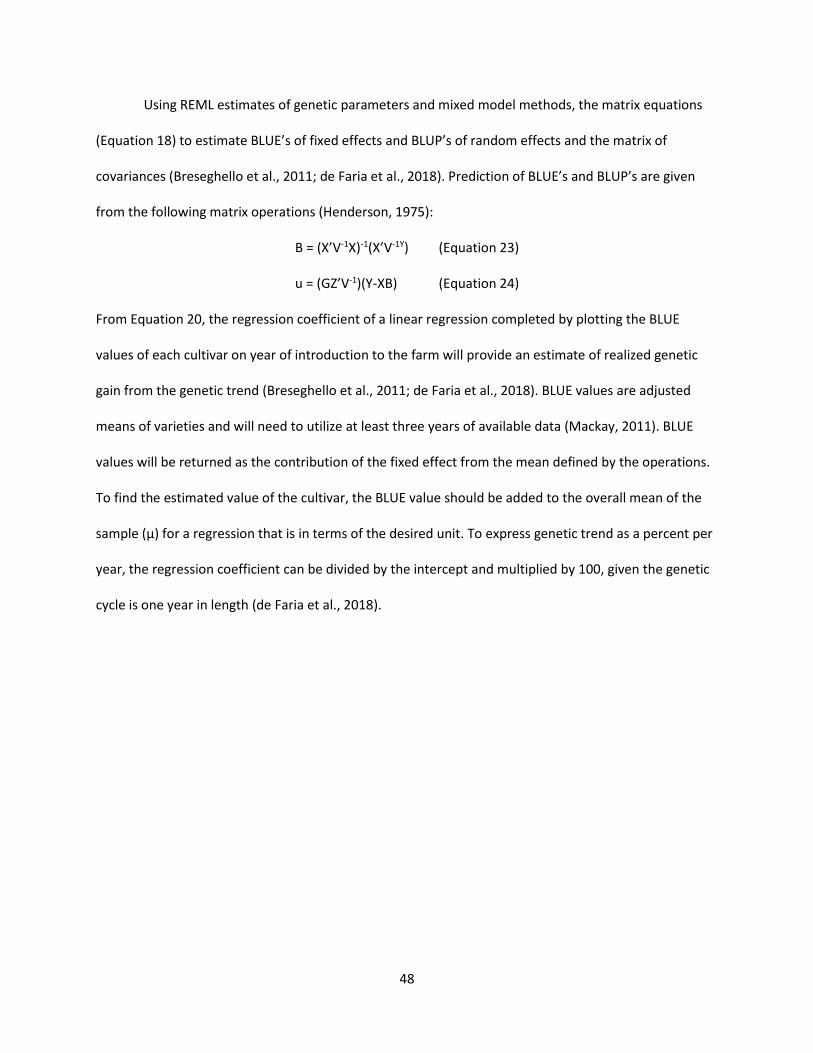
48

Using REML estimates of genetic parameters and mixed model methods, the matrix equations

(Equation 18) to estimate BLUE’s of fixed effects and BLUP’s of random effects and the matrix of

covariances (Breseghello et al., 2011; de Faria et al., 2018). Prediction of BLUE’s and BLUP’s are given

from the following matrix operations (Henderson, 1975):

B = (X’V-1X)-1(X’V-1Y) (Equation 23)

u = (GZ’V-1)(Y-XB) (Equation 24)

From Equation 20, the regression coefficient of a linear regression completed by plotting the BLUE

values of each cultivar on year of introduction to the farm will provide an estimate of realized genetic

gain from the genetic trend (Breseghello et al., 2011; de Faria et al., 2018). BLUE values are adjusted

means of varieties and will need to utilize at least three years of available data (Mackay, 2011). BLUE

values will be returned as the contribution of the fixed effect from the mean defined by the operations.

To find the estimated value of the cultivar, the BLUE value should be added to the overall mean of the

sample (µ) for a regression that is in terms of the desired unit. To express genetic trend as a percent per

year, the regression coefficient can be divided by the intercept and multiplied by 100, given the genetic

cycle is one year in length (de Faria et al., 2018).

49

GLOSSARY

abiotic non-living; not derived from living organisms additive genetic effect a portion of the genotype influencing phenotype. The sum of alleles within an

individual that contribute a fixed value to a quantitative trait or phenotype. Additive genetic effects can be passed from parents to offspring

allele one of two or more alternate forms of a gene analysis of variance (ANOVA) collection of statistical models and associated estimation procedures used to

analyze the differences among group means in a sample biotic living; relating to living things block division of experimental area if variability exists to create uniform subunits Best Linear Unbiased Estimator (BLUE) estimator of random effects from procedures created by C.R.

Henderson within a mixed model Best Linear Unbiased Predictor (BLUP) predictor of fixed effects from procedures created by C.R. Henderson

within a mixed model breeding value the additive genetic effect of genotype an individual can pass to offspring. The value of genes

to progeny complete block contains all treatments being evaluated. Each treatment occurs once within each block correlation statistical measure of the degree to which two variables vary together. Indicates both strength

and direction of the linear relationship between two variables. Correlation is a function of the covariance

covariance statistical measure of the interrelationship between two variables. Indicates the direction of the

linear relationship between variables cultivar a group of plants within a species that has a distinguishing set of characteristics from other groups

within the species; a subdivision of species for taxonomic classification. May be used interchangeably with the term variety. Note that in certain cases variety refers to a naturally occurs distinct species while cultivar refers to a distinct species as a result of artificial human selection

cycle of selection time required to generate breeding individuals or groups, evaluate phenotypic and/or

genotypic data of individuals or groups, select the best individual or groups to recombine, and then recombine individuals or groups by shuffling the allelic combinations through breeding methods

degrees of freedom number of values in the final calculation of a statistic that are free to vary dependent variable variable whose value depends on how the independent variable is manipulated

50

dominance certain alleles being expressed over other alleles, may be partial or complete dominance genetic effect a portion of the genotype influencing phenotype. The effect of dominance on a

quantitative trait or phenotype epistasis interactions between alleles at two or more loci that control the expression of a trait or

characteristic epistatic genetic effect a portion of the genotype influencing phenotype. The effect of epistasis on a

quantitative trait or phenotype experimental error difference between an experimental value and the actual value experimental unit is the unit of experimental material which is randomly assigned to receive a treatment factor a classification or categorical variable which can take one or more values called levels factorial experiment treatments are combinations of two or more levels of factors fixed effect effects within a mathematical model. Fixed effects represent groups for which the differences

between groups is of interest only to this experiment. There is no intention of using the results of the experiment to infer outcomes in any other experiment or under any other conditions. From a technical perspective fixed effects do not have a covariance that needs to be estimated

gamete a mature haploid male or female germ cell gametic phase disequilibrium non-random associated or correlation between two loci gene genetic factor that helps determine a trait or characteristic. May be defined as the molecular sequence

of DNA that is transcribed into RNA genetic gain the improvement in average genetic value of a population with each cycle of selection; response

to selection for additive genetic variance genetic trend estimation of realized changes in genotypic values over multiple cycles genome genetic material of an organism genotype set of genes possessed by an individual organism; genetic contribution to a trait or characteristic haplotype a specific set of linked genetic variants or alleles on a single chromosome or part of a chromosome heritability portion of the phenotypic variation that is due to the genetic differences heritability, broad-sense ratio of total genetic variance to phenotypic variance heritability, narrow-sense ratio of only the additive portion of genetic variance to phenotypic variance

51

incomplete block does not contain all treatments within a block independent variable variable that is manipulated in an experiment infinitesimal model a model developed by Ronald A. Fisher where the variation of a quantitative trait is

influenced by an infinite number of genes; each gene makes an infinitesimal contribution to the trait linear model linear regression model; linear approach to model the relationship between a dependent

variable and independent variable. Relationships are modeled using predictors which are estimated from the data within the model

linkage disequilibrium nonrandom association or correlation between two or more loci on the same

chromosome locus (plural loci) gene locations on chromosomes mass selected group superior individuals selected for breeding based on phenotype mean central value of a discrete set of numbers found by summing all values and dividing by the number of

values mixed linear model a linear model containing both fixed and random effects model equation or set of equations that describe, represent, or approximate the physical, chemical, or

biological (genetic) states of the evaluated entities parameter numerical characteristic of a statistical population or a statistical model phenotype physical appearance of a trait or characteristic; expression of genotype, non-genetic factors, and

their interactions plot an experimental unit in field experiments polygenetic inheritance many genes each with a small effect control a trait precision measurement of the reproducibility of a set of measures qualitative characteristic phenotypic variation among genotypes is not continuous and can be separated into

discrete classes qualitative genetics genetics dealing with discrete traits or characteristics qualitative trait a discrete trait or characteristic is influenced by one or a small number of alleles and loci quantitative characteristic phenotypic variation among genotypes is continuous and cannot be separated into

discrete classes quantitative genetics genetics dealing with continuously varying traits or characteristics

52

quantitative trait a continuous trait or characteristic is generally influenced by many alleles and multiple loci.

The locations of the alleles and loci within the genome are mostly unknown and the effects of individual alleles and their interactions are the subject of discovery research but are mostly unknown. In addition to being influenced by many alleles and loci, quantitative traits are influenced by non-genetic factors and the interaction of genetic and non-genetic factors

random effect effects within a mathematical model. Random effects assume that the sources of variability

represented by the parameters in the model are from a sample of the population. The purpose is to draw inferences from the experiment to a larger population from which the samples were drawn. Random effects require an estimate of covariance among members

randomization application of treatments at random to experimental units

replication application of each treatment to multiple experimental units residual error difference between the observed and value predicted through a model Restricted Maximum Likelihood (REML) Algorithm that estimates variances of a mathematical model by

estimating population parameters that would give the highest likelihood of leading to the observed data with adjustment for degrees of freedom

selection differential average performance of the selected parents versus the overall population mean selection intensity the percentage of individuals that are selected for recombination or breeding single-factor experiment one factor differs between treatments while holding all other factors constant stabilizing selection selection of the population is toward the mean value of a trait causing less extreme

distribution trait a specific characteristic of an organism. Determined by genetics and non-genetic factors as well as their

interactions. truncation selection selection units are ranked based on selection criteria and all those above or below a

certain threshold are selected variance how spread out data is from mean. Higher the variance the more spread out the data is. Lower the

variance the closer to the mean. Variance can be calculated by first taking every number in a data set and subtracting the mean. These values are squares then summed. This value is then divided by the total number of values in the data set

variation differences among cultivars due to genotype, environment, and genotype and environmental

interaction

53

variety a group of plants within a species that has a distinguishing set of characteristics from other groups within the species; a subdivision of species for taxonomic classification. May be used interchangeably with the term cultivar. Note that in certain cases variety refers to a naturally occurs distinct species while cultivar refers to a distinct species as a result of artificial human selection

54

BIBLIOGRAPHY

Barton, N. H., Etheridge, A. M., & Véber, A. (2017). The infinitesimal model: Definition, derivation, and implications. Theoretical Population Biology, 118, 50–73. https://doi.org/10.1016/j.tpb.2017.06.001

Beavis, W.D. (2018). Review Quantitative Methods. Bernardo, R. (1994). Prediction of maize single-cross performance using RFLPs and information from related

hybrids. Crop Science, 34(1), 20-25. https://doi.org/10.2135/cropsci1994.0011183X003400010003x Bernardo, R. (1995). Genetic models for predicting maize single-cross performance in unbalanced yield trial

data. Crop Science, 35(1), 141-147. https://doi.org/10.2135/cropsci1995.0011183X003500010026x Bernardo, R. (2020). Breeding for quantitative traits in plants. (3rd ed.). Stemma Press. Breseghello, F., de Morais, O. P., Pinheiro, P. V., Silva, A. C. S., da Maia de Castro, E., Guimarães, É. P., de

Castro, A. P., Pereira, J. A., de Matos Lopes, A., Utumi, M. M., & de Oliveira, J. P. (2011). Results of 25 years of upland rice breeding in Brazil. Crop Science, 51(3), 914-923. https://doi.org/10.2135/cropsci2010.06.0325

Bulmer, M. G. (1971). The effect of selection on genetic variability. The American Naturalist, 105(943), 201–

211. https://doi.org/10.1086/282718 Bulmer, M.G. (1998). Galton’s law of ancestral heredity. Heredity, 81(5), 579–585.

https://doi.org/10.1038/sj.hdy.6884180 Clewer, A. G., & Scarisbrick, D.H. (2001). Practical statistics and experimental design for plant and crop

science. JWiley.

Cox, T. S., Shroyer, J. P., Ben-Hui, L., Sears, R. G., & Martin, T. J. (1988). Genetic improvement in agronomic traits of hard red winter wheat cultivars from 1919 to 1987. Crop Science, 5, 756–760.

de Faria, L. C., Melo, P. G. S., de Souza, T. L. P. O., Pereira, H. S., & Melo, L. C. (2018). Efficiency of methods for

genetic progress estimation in common bean breeding using database information. Euphytica, 214(9), 164-173. https://doi.org/10.1007/s10681-018-2246-8

de la Vega, A. J., DeLacy, I. H., & Chapman, S. C. (2007). Progress over 20 years of sunflower breeding in

central Argentina. Field Crops Research, 100(1), 61–72. https://doi.org/10.1016/j.fcr.2006.05.012 Discovery Farm Program | Arkansas Agricultural Experiment Station. (n.d.). Retrieved March 24, 2020, from

https://aaes.uark.edu/centers-and-programs/discovery-farm-program/ Discovery Farms Minnesota. (n.d.). Retrieved March 24, 2020, from https://discoveryfarmsmn.org/about-us/ Discovery Farms Washington. (n.d.). Retrieved March 24, 2020, from

https://sites.google.com/site/wadiscoveryfarms/about-df Discovery Farms Wisconsin. (n.d.). Retrieved March 24, 2020, from http://www.uwdiscoveryfarms.org/about

55

Duvick, D. N. (1997). What is yield? In Developing Drought- and Low N-Tolerant Maize.

Proceedings of a Symposium, March 25–29, 1996, CIMMYT, El Batan, Mexico (G. O. Edmeades, M. Banziger, H. R. Mickelson, and C. B. Pena–Valdivia, Eds.), pp. 332–335. CIMMYT, Mexico, D.F.

Duvick, D.N. (2005). The contribution of breeding to yield advances in maize (Zea mays L.). Advances in Agronomy, 86, pp. 83–145. https://doi.org/10.1016/S0065-2113(05)86002-X

Duvick, D. N., Smith, J. S. C., & Cooper, M. (2010). Long-term selection in a commercial hybrid maize breeding

program. In J. Janick (Ed.), Plant Breeding Reviews (pp. 109–151). John Wiley & Sons, Inc. https://doi.org/10.1002/9780470650288.ch4

Eberhart, S. A. (1964). Least squares method for comparing progress among recurrent selection methods.

Crop Science, 4(2), 230–231. https://doi.org/10.2135/cropsci1964.0011183X000400020036x Eccleston, J. A., & Hedayat, A. (1974). On the theory of connected designs: Characterization and optimality.

The Annals of Statistics, 2(6), 1238–1255. https://doi.org/10.1214/aos/1176342876

Falconer, D. S., & Mackay, T. (1996). Introduction to quantitative genetics. (4th ed.). Longman. Farmer-Led Research. (n.d.). Practical Farmers of Iowa. Retrieved March 24, 2020, from

https://practicalfarmers.org/programs/farmer-led-research/ Fehr, W. R. (1991). Principles of cultivar development: theory and technique. Iowa State University. Fisher, R. A. (1918). XV.—The correlation between relatives on the supposition of Mendelian inheritance.

Transactions of the Royal Society of Edinburgh, 52(02), 399–433. https://doi.org/10.1017/S0080456800012163

Fisher, R. A. (1928a). The possible modification of the response of the wild type to recurrent mutations. The

American Naturalist, 62(679), 115–126. https://doi.org/10.1086/280193 Fisher, R. A. (1928b). Two further notes on the origin of dominance. The American Naturalist, 62(683), 571–

574. https://doi.org/10.1086/280234 Fisher, R. A. (1930). The genetical theory of natural selection. Oxford: The Clarendon Press. Galton, F. (1886). Regression towards mediocrity in hereditary stature. The Journal of the Anthropological

Institute of Great Britain and Ireland, 15, 246-263. https://doi.org/10.2307/2841583 Galton, F. (1889). Natural inheritance. Macmillan. http://hdl.handle.net/2027/hvd.tz1mwb Garrick, D. J. (2010). An animal breeding approach to the estimation of genetic and environmental trends

from field populations. Journal of Animal Science, 88 (suppl_13), E3–E10. https://doi.org/10.2527/jas.2009-2329

56

Graybosch, R., Bockelman, H. E., Garland-Campbell, K. A., Garvin, D. F., Regassa, T., Specht, J., & Carver, B. (2014). Wheat. In CSSA Special Publications. American Society of Agronomy, Inc., Crop Science Society of America, Inc., and Soil Science Society of America, Inc. https://doi.org/10.2135/cssaspecpub33.c16

Hallauer, A. R., Carena, M. J., & Miranda Filho, J. B. (2010). Quantitative genetics in maize breeding (3rd ed.).

Springer. Hazel, L. N., & Lush, J. L. (1942). The efficiency of three methods of selection. Journal of Heredity, 33(11), 393–

399. https://doi.org/10.1093/oxfordjournals.jhered.a105102 Henderson, C. R. (1975). Best linear unbiased estimation and prediction under a selection model. Biometrics,

31(2), 423-447. https://doi.org/10.2307/2529430 Henderson, C. R. (1985). Best linear unbiased prediction of nonadditive genetic merits in noninbred

populations. Journal of Animal Science, 60(1), 111–117. https://doi.org/10.2527/jas1985.601111x Hill, W. G. (2014). Applications of population genetics to animal breeding, from Wright, Fisher and Lush to

genomic prediction. Genetics, 196(1), 1–16. https://doi.org/10.1534/genetics.112.147850 Hill, W. G., & Kirkpatrick, M. (2010). What animal breeding has taught us about evolution. Annual Review of

Ecology, Evolution, and Systematics, 41(1), 1–19. https://doi.org/10.1146/annurev-ecolsys-102209-144728

Hulke, B. S., Kleingartner, L. W., Smith, S., Diers, B., Specht, J., & Carver, B. (2014). Sunflower. In CSSA Special

Publications. American Society of Agronomy, Inc., Crop Science Society of America, Inc., and Soil Science Society of America, Inc. https://doi.org/10.2135/cssaspecpub33.c15

Laidig, F., Piepho, H.-P., Drobek, T., & Meyer, U. (2014). Genetic and non-genetic long-term trends of 12

different crops in German official variety performance trials and on-farm yield trends. Theoretical and Applied Genetics, 127(12), 2599–2617. https://doi.org/10.1007/s00122-014-2402-z

Laidig, F., Piepho, H.-P., Rentel, D., Drobek, T., & Meyer, U. (2017). Breeding progress, genotypic and

environmental variation and correlation of quality traits in malting barley in German official variety trials between 1983 and 2015. Theoretical and Applied Genetics, 130(11), 2411–2429. https://doi.org/10.1007/s00122-017-2967-4

Laidig, F., Piepho, H.-P., Rentel, D., Drobek, T., Meyer, U., & Huesken, A. (2017a). Breeding progress,

environmental variation and correlation of winter wheat yield and quality traits in German official variety trials and on-farm during 1983–2014. Theoretical and Applied Genetics, 130(1), 223–245. https://doi.org/10.1007/s00122-016-2810-3

Laidig, F., Piepho, H.-P., Rentel, D., Drobek, T., Meyer, U., & Huesken, A. (2017b). Breeding progress, variation,

and correlation of grain and quality traits in winter rye hybrid and population varieties and national on-farm progress in Germany over 26 years. Theoretical and Applied Genetics, 130(5), 981–998. https://doi.org/10.1007/s00122-017-2865-9

57

Littell, R. C. (2002). Analysis of unbalanced mixed model data: A case study comparison of ANOVA versus REML/GLS. Journal of Agricultural, Biological, and Environmental Statistics, 7(4), 472-490. https://doi.org/10.1198/108571102816

Lush, J. L. (1945). Animal breeding plans. (3rd Ed.) The Iowa State Collegiate Press, Inc. Lush, J. L., (1948). The genetics of populations, (Special report 94). Iowa State College, College of Agriculture. Lush, J. L. (1994). The genetics of populations (Rev. Special report 94). Iowa Agriculture and Home Economics

Experiment Station. Mackay, I., Horwell, A., Garner, J., White, J., McKee, J., & Philpott, H. (2011). Reanalyses of the historical series

of UK variety trials to quantify the contributions of genetic and environmental factors to trends and variability in yield over time. Theoretical and Applied Genetics, 122(1), 225–238. https://doi.org/10.1007/s00122-010-1438-y

Magnello, M. E. (1998). Karl Pearson’s mathematization of inheritance: From ancestral heredity to Mendelian

genetics (1895-1909). Annals of Science, 55(1), 35-94. https://doi.org/10.1080/00033799800200111

Motulsky, H. (2014). Intuitive biostatistics: A nonmathematical guide to statistical thinking. (Completely rev. 2nd ed.). Oxford University Press.

North Dakota Discovery Farms. (n.d.). Retrieved March 24, 2020, from https://www.ag.ndsu.edu/df

Pearson, K. (1904). III. Mathematical contributions to the theory of evolution. XII. On a generalised theory of

alternative Inheritance, with special reference to Mendel’s laws. Philosophical Transactions of the Royal Society of London. Series A, Containing Papers of a Mathematical or Physical Character, 203, 53–86. https://doi.org/10.1098/rsta.1904.0015

Piepho, H.P., Laidig, F., Drobek, T., & Meyer, U. (2014). Dissecting genetic and non-genetic sources of long-term yield trend in German official variety trials. Theoretical and Applied Genetics, 127(5), 1009–1018. https://doi.org/10.1007/s00122-014-2275-1

Provine, W. B. (1971). The origins of theoretical population genetics. University of Chicago Press. R Development Core Team. (2016). A language and environment for statistical computing. R Foundation for

Statistical Computing. http://www.R-project.org/ Research Protocols. (n.d.). Practical Farmers of Iowa. Retrieved March 19, 2020, from

https://practicalfarmers.org/programs/farmer-led-research/research-protocols/ Rutkoski, J. E. (2019a). Estimation of realized rates of genetic gain and indicators for breeding program

assessment. Crop Science, 59(3), 981–993. https://doi.org/10.2135/cropsci2018.09.0537 Rutkoski, J. E. (2019b). Chapter Four—A practical guide to genetic gain. (D. L. Sparks, Ed.), Advances in

Agronomy (Vol. 157, pp. 217–249). Academic Press. https://doi.org/10.1016/bs.agron.2019.05.001

58

Shelton, A. C., & Tracy, W. F. (2017). Cultivar development in the U.S. public sector. Crop Science, 57(4), 1823–1835. https://doi.org/10.2135/cropsci2016.11.0961

Smith, S., Cooper, M., Gogerty, J., Löffler, C., Borcherding, D., Wright, K., Smith, S., Diers, B., Specht, J., &

Carver, B. (2014). Maize. In CSSA Special Publications. American Society of Agronomy, Inc., Crop Science Society of America, Inc., and Soil Science Society of America, Inc. https://doi.org/10.2135/cssaspecpub33.c6

Thompson, R. (2008). Estimation of quantitative genetic parameters. Proceedings of the Royal Society B:

Biological Sciences, 275(1635), 679–686. https://doi.org/10.1098/rspb.2007.1417 Vandemark, G. J., Brick, M. A., Osorno, J. M., Kelly, J. D., Urrea, C. A., Smith, S., Diers, B., Specht, J., & Carver,

B. (2014). Edible grain legumes. In CSSA Special Publications. American Society of Agronomy, Inc., Crop Science Society of America, Inc., and Soil Science Society of America, Inc. https://doi.org/10.2135/cssaspecpub33.c5

Wright, S. (1920). The relative importance of heredity and environment in determining the piebald pattern of

guinea-pigs. Proceedings of the National Academy of Sciences of the United States of America, 6(6), 320–332. https://doi.org/10.1073/pnas.6.6.320

Wright, S. (1921a). Systems of mating. I. The biometric relations between parent and offspring. Genetics, 6(2), 111–123.

Wright, S. (1921b). Systems of mating. II. The effects of inbreeding on the genetic composition of a

population. Genetics, 6(2), 124–143. Wright, S. (1921c). Systems of mating. III. Assortative mating based on somatic resemblance. Genetics, 6(2),

144–161. Wright, S. (1921d). Systems of mating. IV. The effects of selection. Genetics, 6(2), 162–166. Wright, S. (1921e). Systems of mating. V. General considerations. Genetics, 6(2), 167–178. Wright, S. (1929). Fisher’s theory of dominance. The American Naturalist, 63(686), 274–279.

https://doi.org/10.1086/280260 Yule, G. U. (1902). Mendel’s laws and their probable relations to intra-racial heredity. The New Phytologist,

1(9), 193–207.