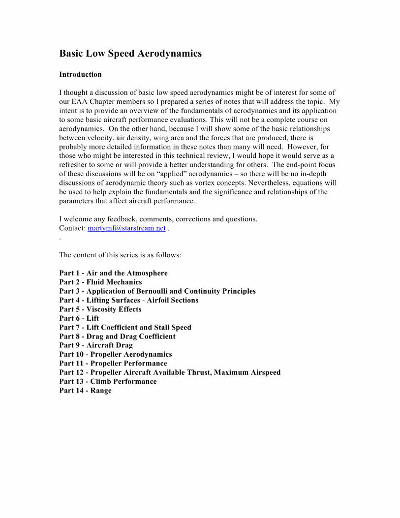
Basic Low Speed Aerodynamics Introduction I thought a discussion of basic low speed aerodynamics might be of interest for some of our EAA Chapter members so I prepared a series of notes that will address the topic. My intent is to provide an overview of the fundamentals of aerodynamics and its application to some basic aircraft performance evaluations. This will not be a complete course on aerodynamics. On the other hand, because I will show some of the basic relationships between velocity, air density, wing area and the forces that are produced, there is probably more detailed information in these notes than many will need. However, for those who might be interested in this technical review, I would hope it would serve as a refresher to some or will provide a better understanding for others. The end-point focus of these discussions will be on “applied” aerodynamics – so there will be no in-depth discussions of aerodynamic theory such as vortex concepts. Nevertheless, equations will be used to help explain the fundamentals and the significance and relationships of the parameters that affect aircraft performance. I welcome any feedback, comments, corrections and questions. Contact: martymf@starstream.net . . The content of this series is as follows: Part 1 - Air and the Atmosphere Part 2 - Fluid Mechanics Part 3 - Application of Bernoulli and Continuity Principles Part 4 - Lifting Surfaces - Airfoil Sections Part 5 - Viscosity Effects Part 6 - Lift Part 7 - Lift Coefficient and Stall Speed Part 8 - Drag and Drag Coefficient Part 9 - Aircraft Drag Part 10 - Propeller Aerodynamics Part 11 - Propeller Performance Part 12 - Propeller Aircraft Available Thrust, Maximum Airspeed Part 13 - Climb Performance Part 14 - Range

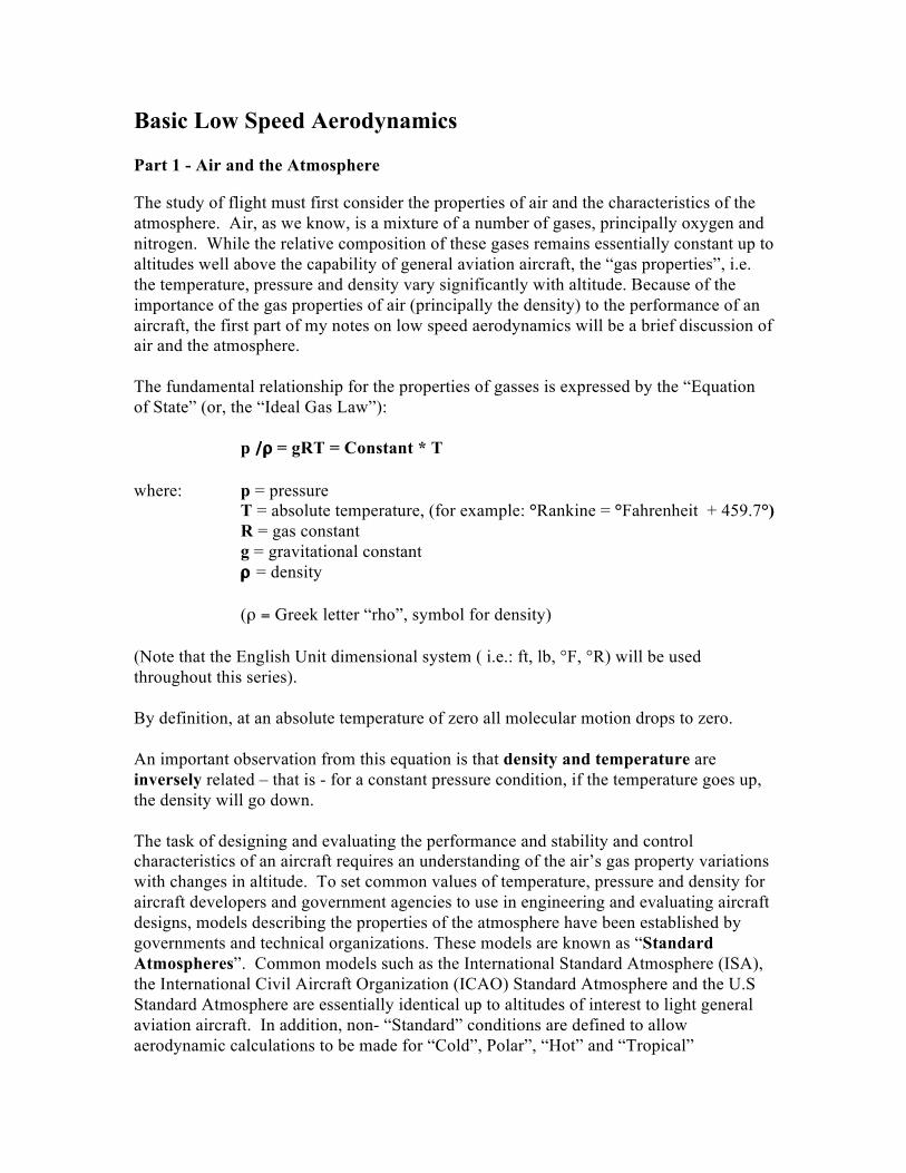
Basic Low Speed Aerodynamics Part 1 - Air and the Atmosphere The study of flight must first consider the properties of air and the characteristics of the atmosphere. Air, as we know, is a mixture of a number of gases, principally oxygen and nitrogen. While the relative composition of these gases remains essentially constant up to altitudes well above the capability of general aviation aircraft, the “gas properties”, i.e. the temperature, pressure and density vary significantly with altitude. Because of the importance of the gas properties of air (principally the density) to the performance of an aircraft, the first part of my notes on low speed aerodynamics will be a brief discussion of air and the atmosphere. The fundamental relationship for the properties of gasses is expressed by the “Equation of State” (or, the “Ideal Gas Law”): p /ρ = gRT = Constant * T where: p = pressure

T = absolute temperature, (for example: °Rankine = °Fahrenheit + 459.7°) R = gas constant g = gravitational constant

ρ = density

(ρ = Greek letter “rho”, symbol for density)

(Note that the English Unit dimensional system ( i.e.: ft, lb, °F, °R) will be used throughout this series). By definition, at an absolute temperature of zero all molecular motion drops to zero.

An important observation from this equation is that density and temperature are inversely related – that is - for a constant pressure condition, if the temperature goes up, the density will go down. The task of designing and evaluating the performance and stability and control characteristics of an aircraft requires an understanding of the air’s gas property variations with changes in altitude. To set common values of temperature, pressure and density for aircraft developers and government agencies to use in engineering and evaluating aircraft designs, models describing the properties of the atmosphere have been established by governments and technical organizations. These models are known as “Standard Atmospheres”. Common models such as the International Standard Atmosphere (ISA), the International Civil Aircraft Organization (ICAO) Standard Atmosphere and the U.S Standard Atmosphere are essentially identical up to altitudes of interest to light general aviation aircraft. In addition, non- “Standard” conditions are defined to allow aerodynamic calculations to be made for “Cold”, Polar”, “Hot” and “Tropical”

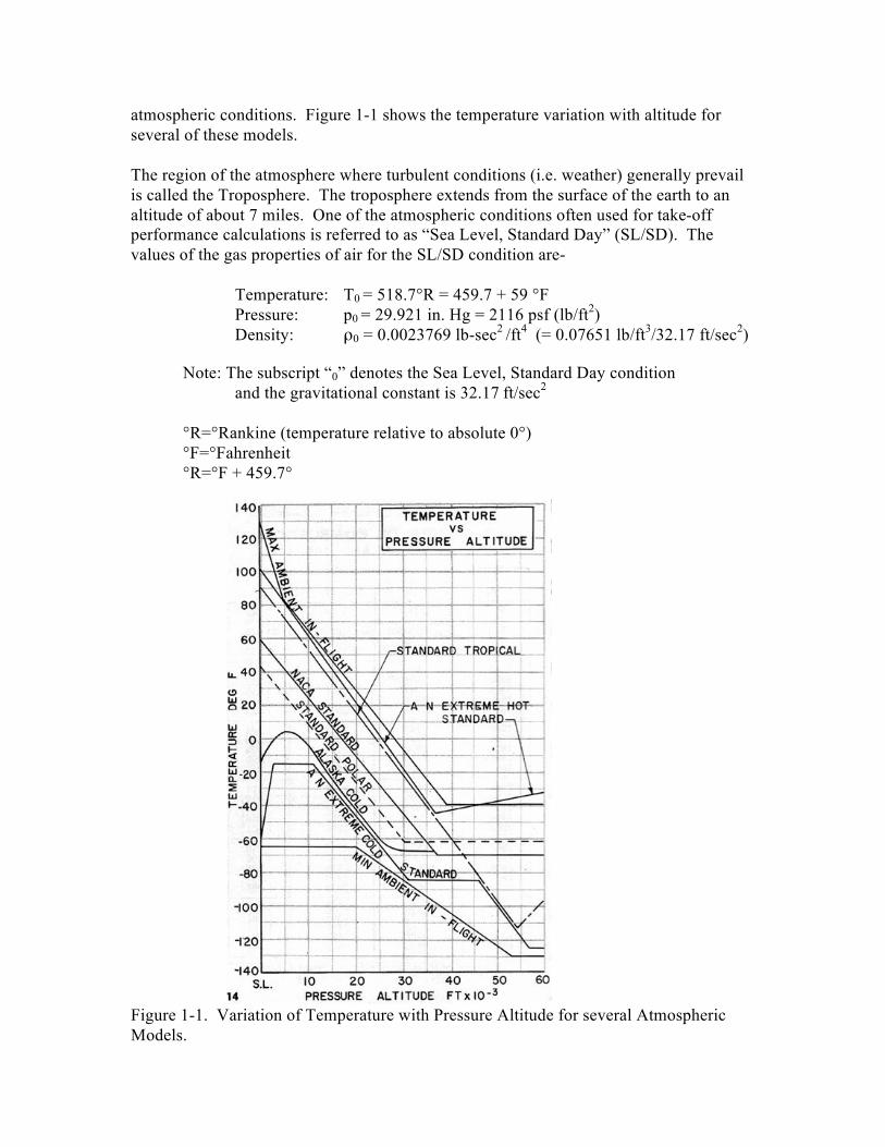
atmospheric conditions. Figure 1-1 shows the temperature variation with altitude for several of these models. The region of the atmosphere where turbulent conditions (i.e. weather) generally prevail is called the Troposphere. The troposphere extends from the surface of the earth to an altitude of about 7 miles. One of the atmospheric conditions often used for take-off performance calculations is referred to as “Sea Level, Standard Day” (SL/SD). The values of the gas properties of air for the SL/SD condition are- Temperature: T0 = 518.7°R = 459.7 + 59 °F Pressure: p0 = 29.921 in. Hg = 2116 psf (lb/ft2) Density: ρ0 = 0.0023769 lb-sec2 /ft4 (= 0.07651 lb/ft3/32.17 ft/sec2) Note: The subscript “0” denotes the Sea Level, Standard Day condition and the gravitational constant is 32.17 ft/sec2

°R=°Rankine (temperature relative to absolute 0°) °F=°Fahrenheit

°R=°F + 459.7°

Figure 1-1. Variation of Temperature with Pressure Altitude for several Atmospheric Models.

The following table presents an example of the standard variation of temperature, pressure and density with altitude from sea level to 10,000 ft and is listed as changes relative to conditions at sea level. Note that the temperature ratio is based on “absolute temperature”, mentioned above, for which absolute zero is - 459.7° F. Atmospheric Conditions Compared to Sea Level: Altitude Temperature* Pressure Density ft Ratio Ratio Ratio 0 1.0 1.0 1.0 2000 0.986 0.928 0.943 4000 0.973 0.834 0.888 6000 0.959 0.801 0.835 8000 0.945 0.743 0.786 10000 0.931 0.688 0.739 * Absolute Temperature Ratio Relative to conditions at sea level, temperature, pressure and density all decrease with increasing altitude – but at different rates.

Basic Low Speed Aerodynamics Part 2 - Fluid Mechanics Note: Aerodynamics is a subset of fluid dynamics. Air is a “fluid”. Energy Conservation

Figure 2-1. Daniel Bernoulli In the 1700s Daniel Bernoulli, a Dutch-born member of a Swiss mathematical family, determined that the total energy in a moving fluid stream remains constant at any point in the flow. Based on this insight, Bernoulli stipulated that the sum of the “Pressure Energy” (i.e. the static pressure) and the “Kinetic Energy” (related to the motion of the fluid) along a “streamline” must remain constant. The term for the static pressure in the fluid is p and the “Kinetic Energy” (or “dynamic pressure”) in the fluid is defined by ρV2/2 (or “q”), where ρ is the density of the fluid and V is the velocity of the fluid’s motion.

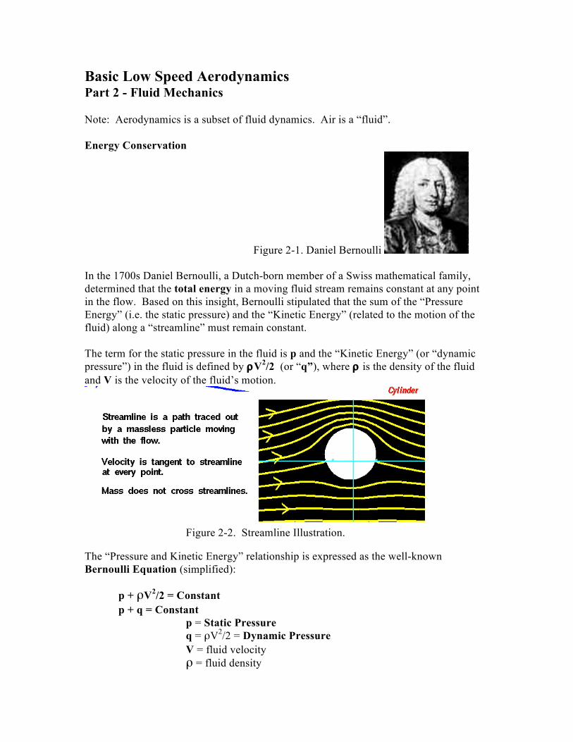
Figure 2-2. Streamline Illustration. The “Pressure and Kinetic Energy” relationship is expressed as the well-known Bernoulli Equation (simplified): p + ρV2/2 = Constant p + q = Constant p = Static Pressure q = ρV2/2 = Dynamic Pressure V = fluid velocity ρ = fluid density

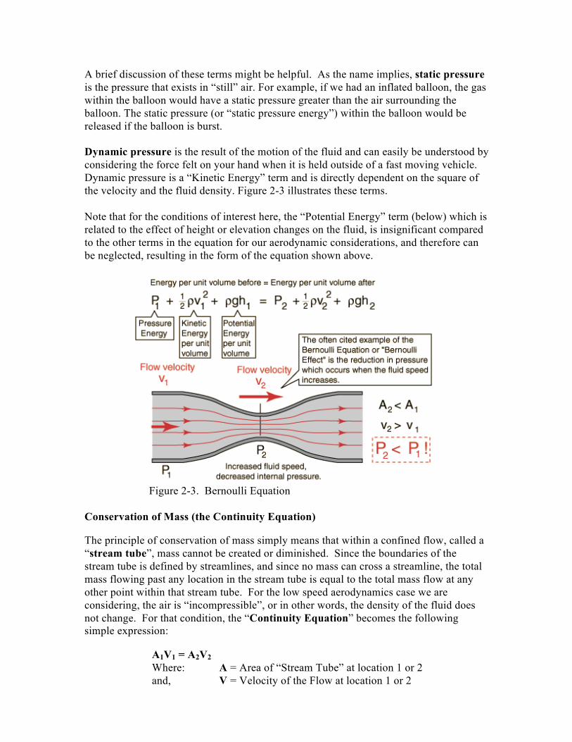
A brief discussion of these terms might be helpful. As the name implies, static pressure is the pressure that exists in “still” air. For example, if we had an inflated balloon, the gas within the balloon would have a static pressure greater than the air surrounding the balloon. The static pressure (or “static pressure energy”) within the balloon would be released if the balloon is burst. Dynamic pressure is the result of the motion of the fluid and can easily be understood by considering the force felt on your hand when it is held outside of a fast moving vehicle. Dynamic pressure is a “Kinetic Energy” term and is directly dependent on the square of the velocity and the fluid density. Figure 2-3 illustrates these terms. Note that for the conditions of interest here, the “Potential Energy” term (below) which is related to the effect of height or elevation changes on the fluid, is insignificant compared to the other terms in the equation for our aerodynamic considerations, and therefore can be neglected, resulting in the form of the equation shown above.

Figure 2-3. Bernoulli Equation Conservation of Mass (the Continuity Equation) The principle of conservation of mass simply means that within a confined flow, called a “stream tube”, mass cannot be created or diminished. Since the boundaries of the stream tube is defined by streamlines, and since no mass can cross a streamline, the total mass flowing past any location in the stream tube is equal to the total mass flow at any other point within that stream tube. For the low speed aerodynamics case we are considering, the air is “incompressible”, or in other words, the density of the fluid does not change. For that condition, the “Continuity Equation” becomes the following simple expression: A1V1 = A2V2 Where: A = Area of “Stream Tube” at location 1 or 2 and, V = Velocity of the Flow at location 1 or 2

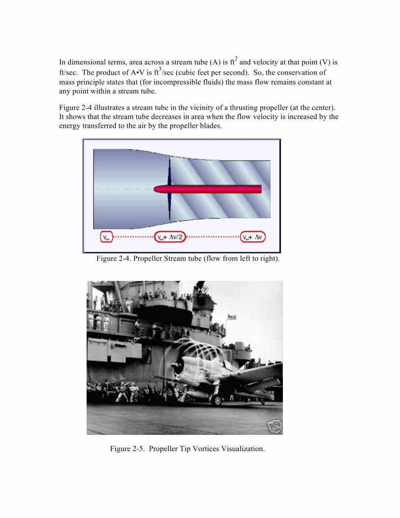
In dimensional terms, area across a stream tube (A) is ft2 and velocity at that point (V) is ft/sec. The product of A•V is ft3/sec (cubic feet per second). So, the conservation of mass principle states that (for incompressible fluids) the mass flow remains constant at any point within a stream tube. Figure 2-4 illustrates a stream tube in the vicinity of a thrusting propeller (at the center). It shows that the stream tube decreases in area when the flow velocity is increased by the energy transferred to the air by the propeller blades.

Figure 2-4. Propeller Stream tube (flow from left to right).

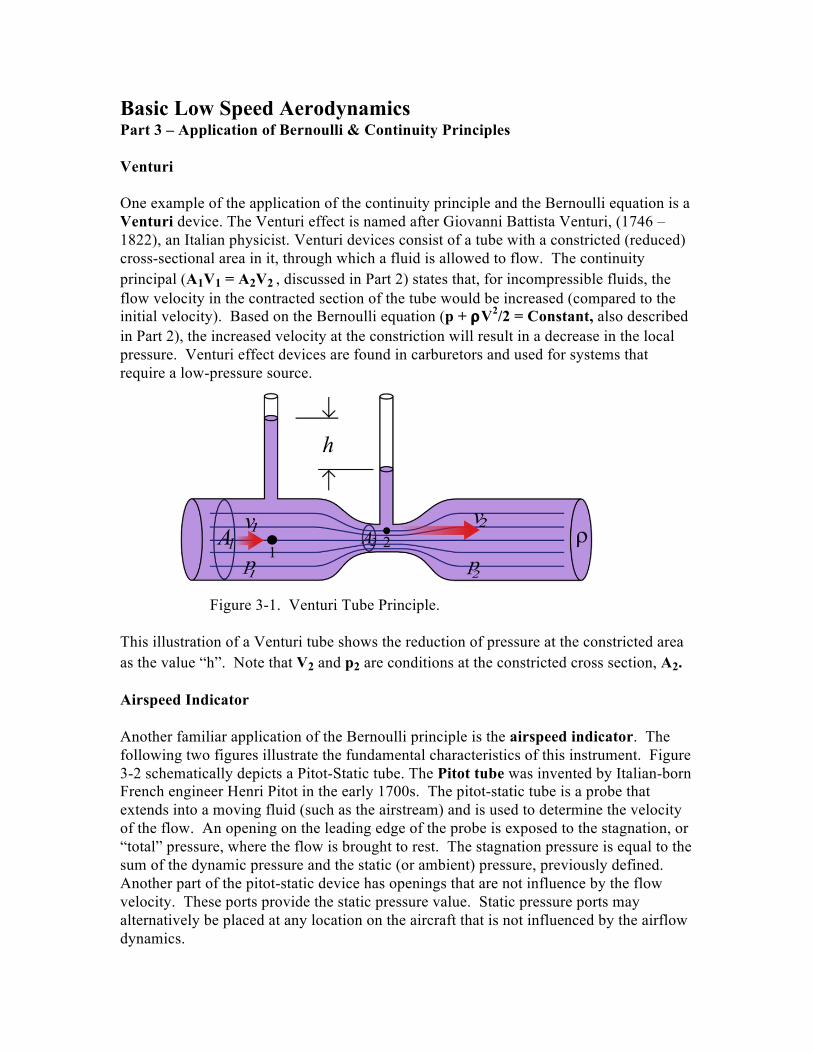
Figure 2-5. Propeller Tip Vortices Visualization.

The contraction of the propeller wake is made visible by condensation of water vapor within the tip vortices (figure 2-5). The propeller tip radius is indicated by the location of the first visible vortex above the fuselage. Subsequent vortices illustrate the reduction of the wake radius. It should be noted that without the presence of the fuselage in the propeller slipstream (aft of the propeller disc) the contraction of the wake would be greater than it appears in this photograph.

Basic Low Speed Aerodynamics Part 3 – Application of Bernoulli & Continuity Principles Venturi One example of the application of the continuity principle and the Bernoulli equation is a Venturi device. The Venturi effect is named after Giovanni Battista Venturi, (1746 –1822), an Italian physicist. Venturi devices consist of a tube with a constricted (reduced) cross-sectional area in it, through which a fluid is allowed to flow. The continuity principal (A1V1 = A2V2 , discussed in Part 2) states that, for incompressible fluids, the flow velocity in the contracted section of the tube would be increased (compared to the initial velocity). Based on the Bernoulli equation (p + ρV2/2 = Constant, also described in Part 2), the increased velocity at the constriction will result in a decrease in the local pressure. Venturi effect devices are found in carburetors and used for systems that require a low-pressure source.

Figure 3-1. Venturi Tube Principle. This illustration of a Venturi tube shows the reduction of pressure at the constricted area as the value “h”. Note that V2 and p2 are conditions at the constricted cross section, A2. Airspeed Indicator Another familiar application of the Bernoulli principle is the airspeed indicator. The following two figures illustrate the fundamental characteristics of this instrument. Figure 3-2 schematically depicts a Pitot-Static tube. The Pitot tube was invented by Italian-born French engineer Henri Pitot in the early 1700s. The pitot-static tube is a probe that extends into a moving fluid (such as the airstream) and is used to determine the velocity of the flow. An opening on the leading edge of the probe is exposed to the stagnation, or “total” pressure, where the flow is brought to rest. The stagnation pressure is equal to the sum of the dynamic pressure and the static (or ambient) pressure, previously defined. Another part of the pitot-static device has openings that are not influence by the flow velocity. These ports provide the static pressure value. Static pressure ports may alternatively be placed at any location on the aircraft that is not influenced by the airflow dynamics.

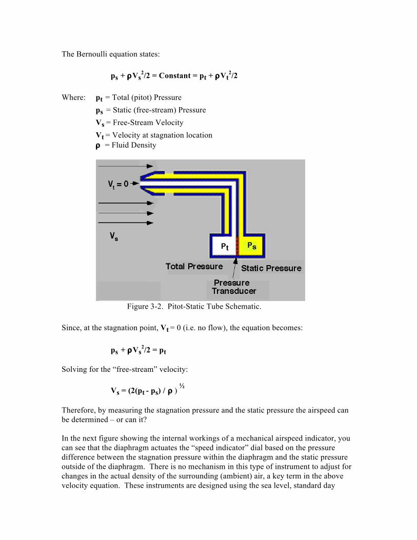
The Bernoulli equation states: ps + ρVs

2/2 = Constant = pt + ρVt2/2

Where: pt

= Total (pitot) Pressure ps

= Static (free-stream) Pressure Vs = Free-Stream Velocity Vt = Velocity at stagnation location ρ = Fluid Density

Figure 3-2. Pitot-Static Tube Schematic. Since, at the stagnation point, Vt = 0 (i.e. no flow), the equation becomes: ps + ρVs

2/2 = pt Solving for the “free-stream” velocity: Vs = (2(pt - ps) / ρ )

½

Therefore, by measuring the stagnation pressure and the static pressure the airspeed can be determined – or can it? In the next figure showing the internal workings of a mechanical airspeed indicator, you can see that the diaphragm actuates the “speed indicator” dial based on the pressure difference between the stagnation pressure within the diaphragm and the static pressure outside of the diaphragm. There is no mechanism in this type of instrument to adjust for changes in the actual density of the surrounding (ambient) air, a key term in the above velocity equation. These instruments are designed using the sea level, standard day

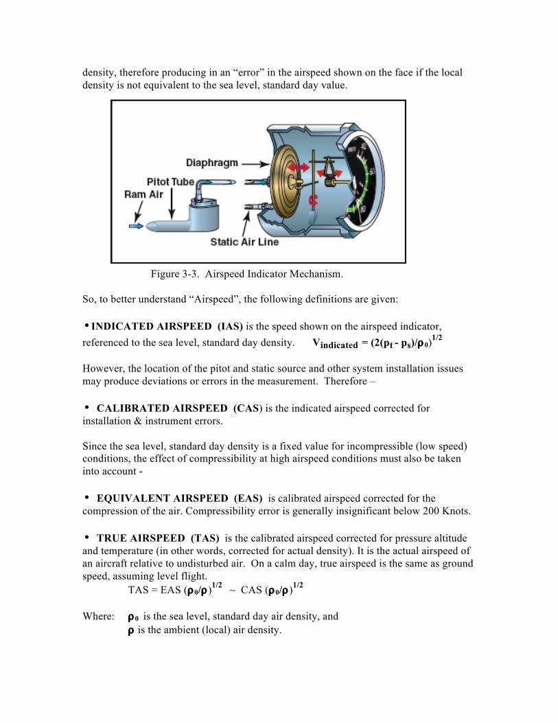
density, therefore producing in an “error” in the airspeed shown on the face if the local density is not equivalent to the sea level, standard day value. Figure 3-3. Airspeed Indicator Mechanism. So, to better understand “Airspeed”, the following definitions are given: •INDICATED AIRSPEED (IAS) is the speed shown on the airspeed indicator, referenced to the sea level, standard day density. Vindicated = (2(pt - ps)/ρ0)

1/2 However, the location of the pitot and static source and other system installation issues may produce deviations or errors in the measurement. Therefore – • CALIBRATED AIRSPEED (CAS) is the indicated airspeed corrected for installation & instrument errors. Since the sea level, standard day density is a fixed value for incompressible (low speed) conditions, the effect of compressibility at high airspeed conditions must also be taken into account - • EQUIVALENT AIRSPEED (EAS) is calibrated airspeed corrected for the compression of the air. Compressibility error is generally insignificant below 200 Knots. • TRUE AIRSPEED (TAS) is the calibrated airspeed corrected for pressure altitude and temperature (in other words, corrected for actual density). It is the actual airspeed of an aircraft relative to undisturbed air. On a calm day, true airspeed is the same as ground speed, assuming level flight. TAS = EAS (ρ0/ρ)1/2 ~ CAS (ρ0/ρ)1/2

Where: ρ0 is the sea level, standard day air density, and ρ is the ambient (local) air density.

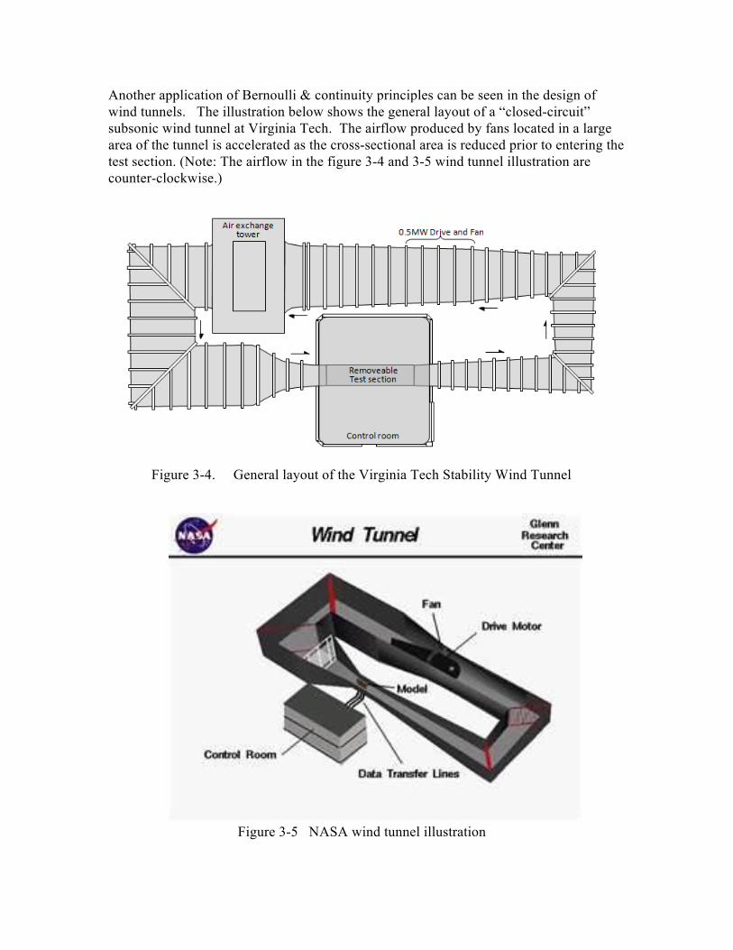
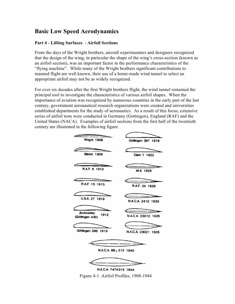
Another application of Bernoulli & continuity principles can be seen in the design of wind tunnels. The illustration below shows the general layout of a “closed-circuit” subsonic wind tunnel at Virginia Tech. The airflow produced by fans located in a large area of the tunnel is accelerated as the cross-sectional area is reduced prior to entering the test section. (Note: The airflow in the figure 3-4 and 3-5 wind tunnel illustration are counter-clockwise.)

Figure 3-4. General layout of the Virginia Tech Stability Wind Tunnel

Figure 3-5 NASA wind tunnel illustration

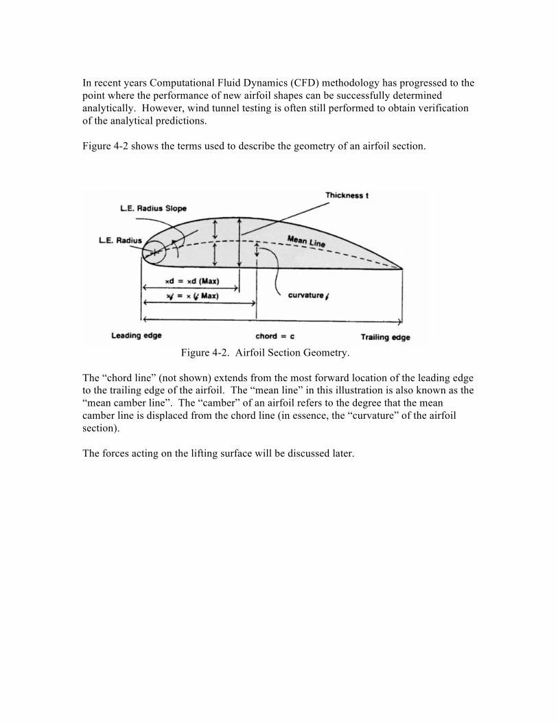
Basic Low Speed Aerodynamics Part 4 - Lifting Surfaces - Airfoil Sections From the days of the Wright brothers, aircraft experimenters and designers recognized that the design of the wing, in particular the shape of the wing’s cross-section (known as an airfoil section), was an important factor in the performance characteristics of the “flying machine”. While many of the Wright brothers significant contributions to manned flight are well known, their use of a home-made wind tunnel to select an appropriate airfoil may not be as widely recognized. For over six decades after the first Wright brothers flight, the wind tunnel remained the principal tool to investigate the characteristics of various airfoil shapes. When the importance of aviation was recognized by numerous countries in the early part of the last century, government aeronautical research organizations were created and universities established departments for the study of aeronautics. As a result of this focus, extensive series of airfoil tests were conducted in Germany (Gottingen), England (RAF) and the United States (NACA). Examples of airfoil sections from the first half of the twentieth century are illustrated in the following figure.

Figure 4-1. Airfoil Profiles, 1908-1944

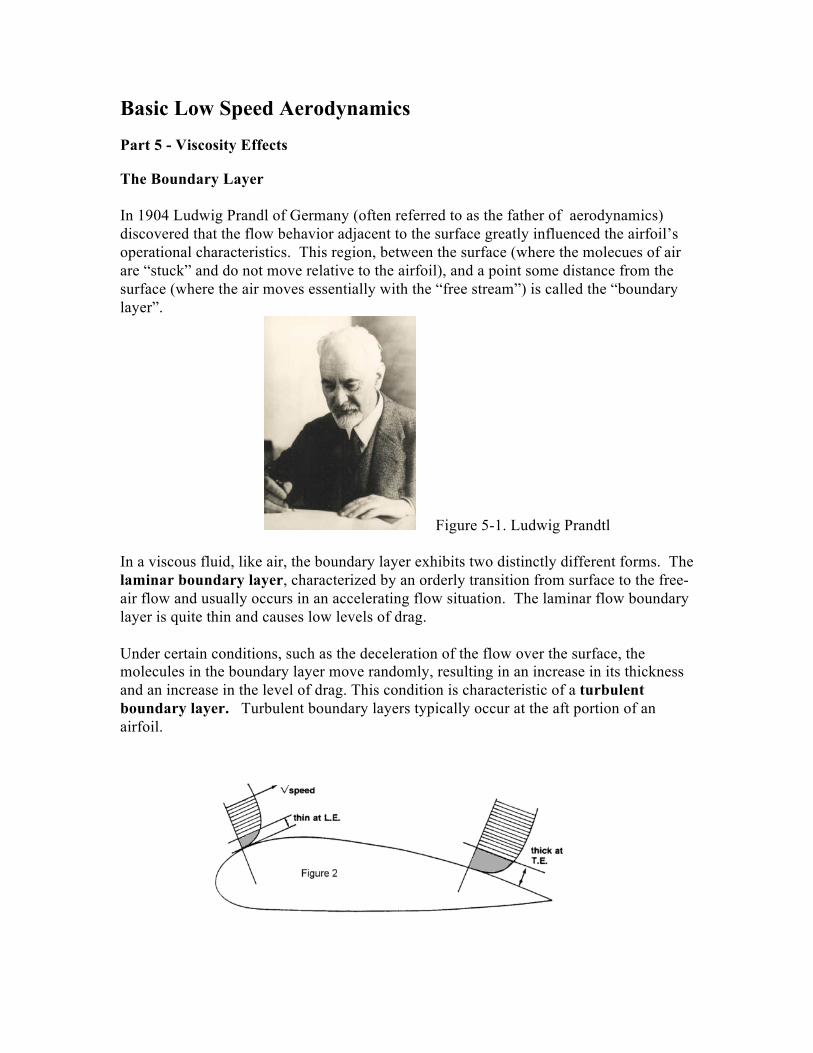
In recent years Computational Fluid Dynamics (CFD) methodology has progressed to the point where the performance of new airfoil shapes can be successfully determined analytically. However, wind tunnel testing is often still performed to obtain verification of the analytical predictions. Figure 4-2 shows the terms used to describe the geometry of an airfoil section.

Figure 4-2. Airfoil Section Geometry.

The “chord line” (not shown) extends from the most forward location of the leading edge to the trailing edge of the airfoil. The “mean line” in this illustration is also known as the “mean camber line”. The “camber” of an airfoil refers to the degree that the mean camber line is displaced from the chord line (in essence, the “curvature” of the airfoil section). The forces acting on the lifting surface will be discussed later.

Basic Low Speed Aerodynamics Part 5 - Viscosity Effects The Boundary Layer In 1904 Ludwig Prandl of Germany (often referred to as the father of aerodynamics) discovered that the flow behavior adjacent to the surface greatly influenced the airfoil’s operational characteristics. This region, between the surface (where the molecues of air are “stuck” and do not move relative to the airfoil), and a point some distance from the surface (where the air moves essentially with the “free stream”) is called the “boundary layer”.

Figure 5-1. Ludwig Prandtl

In a viscous fluid, like air, the boundary layer exhibits two distinctly different forms. The laminar boundary layer, characterized by an orderly transition from surface to the free-air flow and usually occurs in an accelerating flow situation. The laminar flow boundary layer is quite thin and causes low levels of drag. Under certain conditions, such as the deceleration of the flow over the surface, the molecules in the boundary layer move randomly, resulting in an increase in its thickness and an increase in the level of drag. This condition is characteristic of a turbulent boundary layer. Turbulent boundary layers typically occur at the aft portion of an airfoil.

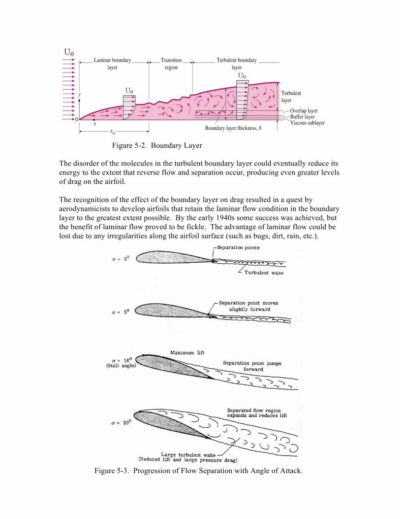
Figure 5-2. Boundary Layer The disorder of the molecules in the turbulent boundary layer could eventually reduce its energy to the extent that reverse flow and separation occur, producing even greater levels of drag on the airfoil. The recognition of the effect of the boundary layer on drag resulted in a quest by aerodynamicists to develop airfoils that retain the laminar flow condition in the boundary layer to the greatest extent possible. By the early 1940s some success was achieved, but the benefit of laminar flow proved to be fickle. The advantage of laminar flow could be lost due to any irregularities along the airfoil surface (such as bugs, dirt, rain, etc.).

Figure 5-3. Progression of Flow Separation with Angle of Attack.

“Rule of Thumb: A laminar flow wing built poorly will often be worse than a turbulent flow wing built poorly.”

And-

“Just remember, put the round end in front and the sharp end in back and you’ll be fine.”

Reynolds Number Boundary Layer Growth and its effect on lift and drag depends on the size of the wing, its velocity, and the viscosity of the fluid the wing is immersed in. In the late 1800s Osborne Reynolds, an Irish-born British fluid dynamics engineer, discovered an important relationship between these parameters. The parameter that bears his name relates a fluid’s inertial forces (velocity*density) to the viscous forces (viscosity/body-length). It is essentially an indicator of the effect of the “scale” of a body moving through the fluid and is used to identify and predict different flow regimes, such as laminar or turbulent flow.

Figure 5-4. Osborne Reynolds Reynolds Number = RN = ρVc/µ

ρ = Density, lb-sec2/ft4

V = Velocity, ft/sec c = Length (chord), ft µ = Absolute Viscosity, lb-sec2/ft2 (Temperature dependant) µ =3.745*10-7 for air at sea level, standard day (µ = Greek letter “mu”)

Simplified, at sea level, standard day:

RN = 9310*Vmph*c For example, at 120 mph, a wing with a 4 ft chord would have a Reynolds Number of 4,470,000, (4.47x106).

To obtain the airfoil performance information that would be appropriate for selected operating conditions (that is: airspeed, wing chord and altitude), airfoil data is measured (in a wind tunnel) or calculated analytically at a specific Reynolds Number. As noted earlier, the size and speed of the aircraft determine the value of the Reynolds Number. Typical values for a range of aircraft applications are shown in the following examples:

Reynolds Numbers of 200,000 or less:

Generally for model airplanes and small UAV (Unmanned Aerial Vehicles). Low Reynolds number airfoils will have relatively low maximum lift coefficients and higher drag than found in higher RN cases.

Reynolds Numbers between about 500K and 7 million:

Usually applies to general aviation; this is the regime where most of the wind tunnel tests have been run.

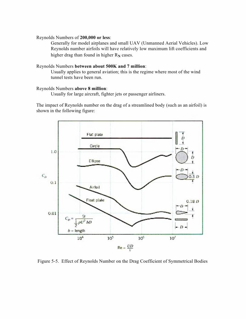
Reynolds Numbers above 8 million: Usually for large aircraft, fighter jets or passenger airliners. The impact of Reynolds number on the drag of a streamlined body (such as an airfoil) is shown in the following figure:

Figure 5-5. Effect of Reynolds Number on the Drag Coefficient of Symmetrical Bodies

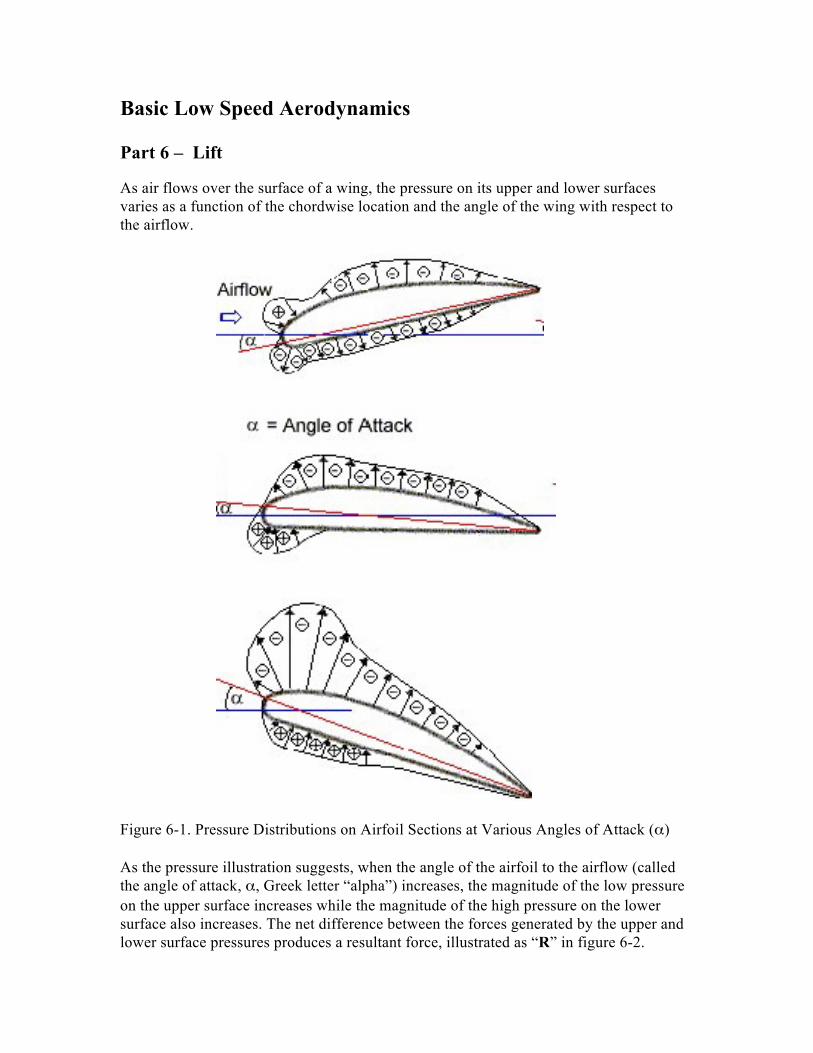
Basic Low Speed Aerodynamics Part 6 – Lift As air flows over the surface of a wing, the pressure on its upper and lower surfaces varies as a function of the chordwise location and the angle of the wing with respect to the airflow.

Figure 6-1. Pressure Distributions on Airfoil Sections at Various Angles of Attack (α) As the pressure illustration suggests, when the angle of the airfoil to the airflow (called the angle of attack, α, Greek letter “alpha”) increases, the magnitude of the low pressure on the upper surface increases while the magnitude of the high pressure on the lower surface also increases. The net difference between the forces generated by the upper and lower surface pressures produces a resultant force, illustrated as “R” in figure 6-2.

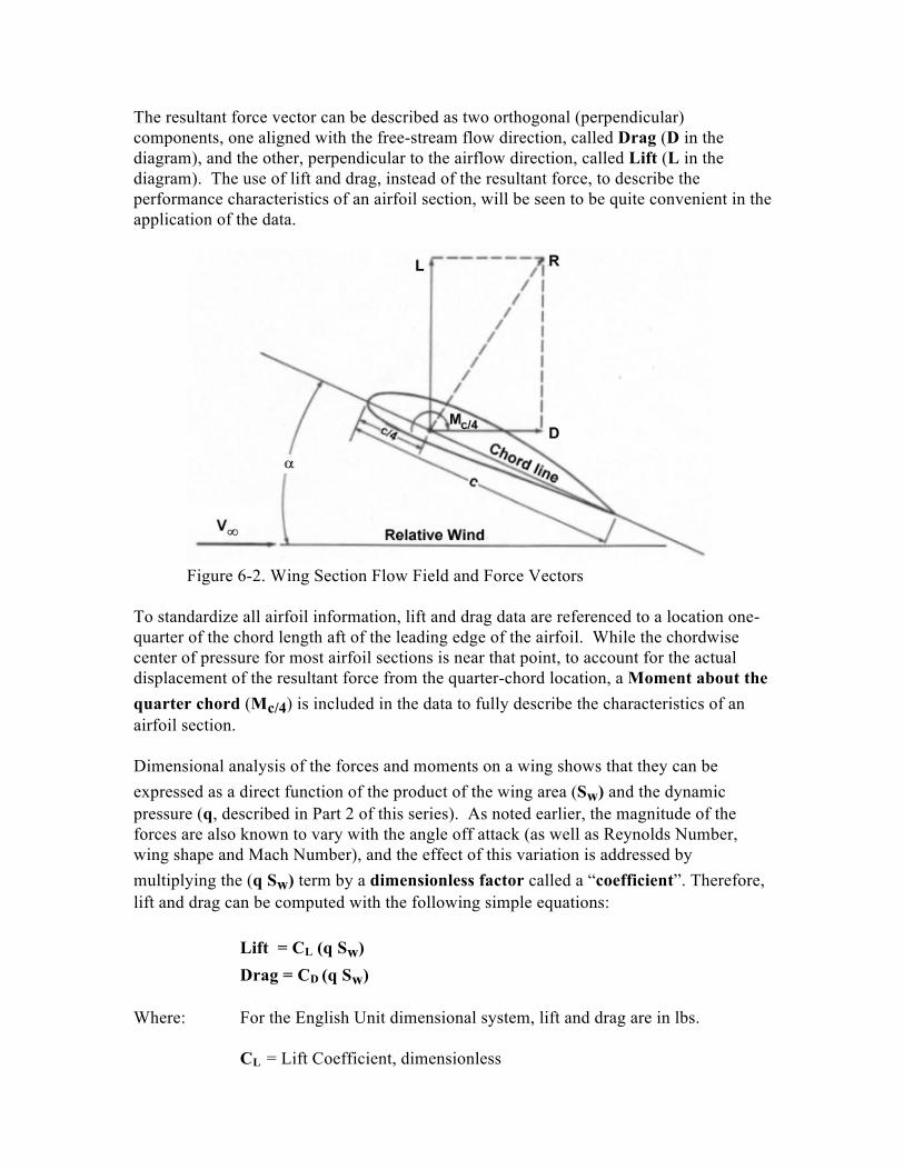
The resultant force vector can be described as two orthogonal (perpendicular) components, one aligned with the free-stream flow direction, called Drag (D in the diagram), and the other, perpendicular to the airflow direction, called Lift (L in the diagram). The use of lift and drag, instead of the resultant force, to describe the performance characteristics of an airfoil section, will be seen to be quite convenient in the application of the data.

Figure 6-2. Wing Section Flow Field and Force Vectors

To standardize all airfoil information, lift and drag data are referenced to a location one-quarter of the chord length aft of the leading edge of the airfoil. While the chordwise center of pressure for most airfoil sections is near that point, to account for the actual displacement of the resultant force from the quarter-chord location, a Moment about the quarter chord (Mc/4) is included in the data to fully describe the characteristics of an airfoil section. Dimensional analysis of the forces and moments on a wing shows that they can be expressed as a direct function of the product of the wing area (Sw) and the dynamic pressure (q, described in Part 2 of this series). As noted earlier, the magnitude of the forces are also known to vary with the angle off attack (as well as Reynolds Number, wing shape and Mach Number), and the effect of this variation is addressed by multiplying the (q Sw) term by a dimensionless factor called a “coefficient”. Therefore, lift and drag can be computed with the following simple equations:

Lift = CL (q Sw) Drag = CD (q Sw)

Where: For the English Unit dimensional system, lift and drag are in lbs.

CL = Lift Coefficient, dimensionless

CD = Drag Coefficient, dimensionless Sw = Wing Area, ft2

q = Dynamic Pressure = ρV2/2, lb/ft2

Similarly, the moment about the quarter chord point can be computed by:

Momentc/4 = Cm-c/4 (q Sw) c

Where: Cm-c/4 = Moment Coefficient, dimensionless

c = wing chord, ft

Basic Low Speed Aerodynamics Part 7 - Lift Coefficient Characteristics

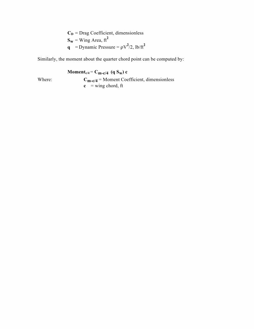
In Part 6 the lift coefficient (CL) was defined as a dimensionless parameter that will yield the magnitude of the lift when multiplied by the wing surface area (Sw) and the dynamic pressure (q) of the inflowing air. An example of the variation of lift coefficient with angle of attack is depicted in figure 7-1. It shows that for low angles of attack the lift coefficient of airfoils operating in the subsonic speed range varies linearly with changes in angle of attack (α). Also illustrated in this figure is the effect of higher angles of attack on the lift coefficient. As α is increased to higher angles the slope of the lift curve begins to level out, eventually reaches a peak value, and then begins to diminish. The reduction of the lift slope and the eventual reduction of lift is due to the separation of the flow (remember the turbulent boundary layer?), a condition referred to as “stall”. The point at which maximum lift coefficient is obtained (in this case a CL of about 1.7) is called (naturally) CL-MAX . This value is usually used when an aircraft’s stall speed is calculated.

Figure 7-1. Typical Lift Coefficient versus Angle of Attack. For many airfoils, stall occurs in the vicinity of a 16° angle of attack. Note that lift does not disappear after stall, it is simply reduced. It is a region, however, that is not desirable for most flight situations – you don’t want to live there. (Later we will see that a significant increase in drag also occurs as stall is approached).

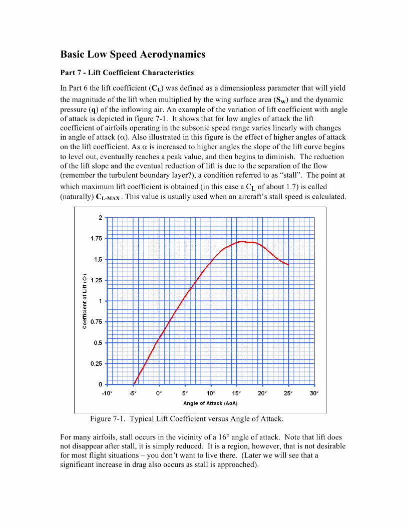
Examples of the effect of the shape of the basic airfoil on the lift coefficient are shown below. The NACA 64-012 airfoil is 12% thick and has 0 camber. The data for the “plain airfoil” shows a maximum CL of about 1.4 at a 13° angle of attack. By altering the shape of the airfoil with devices such as a leading edge slat and a trailing edge flap the maximum lift can be increased significantly.

Figure 7-2. Lift Coefficient versus Angle of Attack for various Airfoil Configurations. These configuration modifications are referred to as “high lift devices” and include, among other things, the use of flaps, slots, slats and boundary layer control, which can be employed either independently or in combination with other devices. Figure 7-3 illustrates the effect of some of these airfoil configuration changes on lift.

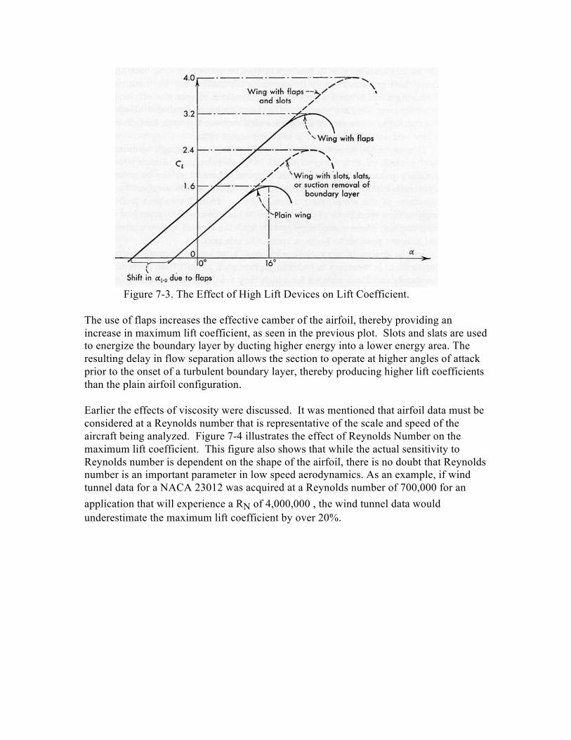
Figure 7-3. The Effect of High Lift Devices on Lift Coefficient. The use of flaps increases the effective camber of the airfoil, thereby providing an increase in maximum lift coefficient, as seen in the previous plot. Slots and slats are used to energize the boundary layer by ducting higher energy into a lower energy area. The resulting delay in flow separation allows the section to operate at higher angles of attack prior to the onset of a turbulent boundary layer, thereby producing higher lift coefficients than the plain airfoil configuration. Earlier the effects of viscosity were discussed. It was mentioned that airfoil data must be considered at a Reynolds number that is representative of the scale and speed of the aircraft being analyzed. Figure 7-4 illustrates the effect of Reynolds Number on the maximum lift coefficient. This figure also shows that while the actual sensitivity to Reynolds number is dependent on the shape of the airfoil, there is no doubt that Reynolds number is an important parameter in low speed aerodynamics. As an example, if wind tunnel data for a NACA 23012 was acquired at a Reynolds number of 700,000 for an application that will experience a RN of 4,000,000 , the wind tunnel data would underestimate the maximum lift coefficient by over 20%.

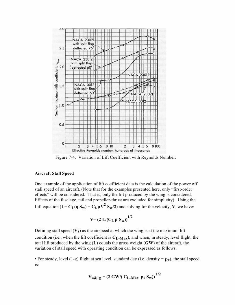
Figure 7-4. Variation of Lift Coefficient with Reynolds Number. Aircraft Stall Speed One example of the application of lift coefficient data is the calculation of the power off stall speed of an aircraft. (Note that for the examples presented here, only “first-order effects” will be considered. That is, only the lift produced by the wing is considered. Effects of the fuselage, tail and propeller-thrust are excluded for simplicity). Using the Lift equation (L= CL(q Sw) = CL ρV2 Sw/2) and solving for the velocity, V, we have: V= (2 L/(CL ρ Sw))1/2

Defining stall speed (VS) as the airspeed at which the wing is at the maximum lift condition (i.e., when the lift coefficient is CL-Max), and when, in steady, level flight, the total lift produced by the wing (L) equals the gross weight (GW) of the aircraft, the variation of stall speed with operating condition can be expressed as follows: • For steady, level (1-g) flight at sea level, standard day (i.e. density = ρ0), the stall speed is: Vs@1g = (2 GW/( CL-Max ρ0 Sw)) 1/2

The actual stall speed can also be dependent on a maneuver, such as a turn, which alters the level of lift required, and on changes in the density due to altitude or temperature variations. • In a 2-g (i.e. L= 2*GW) steady, level turn at a sea level, standard day condition, the stall speed is: Vs@2g = (2*2 GW/( CL-Max ρ0 Sw)) ½ (where GW is the gross weight of the aircraft) or 1.414 times the 1-g (level flight) stall speed at sea level, standard day. • And, for a 2-g steady, level turn at an altitude of 4000 ft, (where the standard day density is .888 of the sea level, standard day density), the stall speed is: Vs@2g,4000’ = (2*2 GW/(0.888 CL-Max ρ0 Sw)) ½ or 1.5 times the 1-g stall speed at sea level, standard day.

Basic Low Speed Aerodynamics

Part 8 – Drag

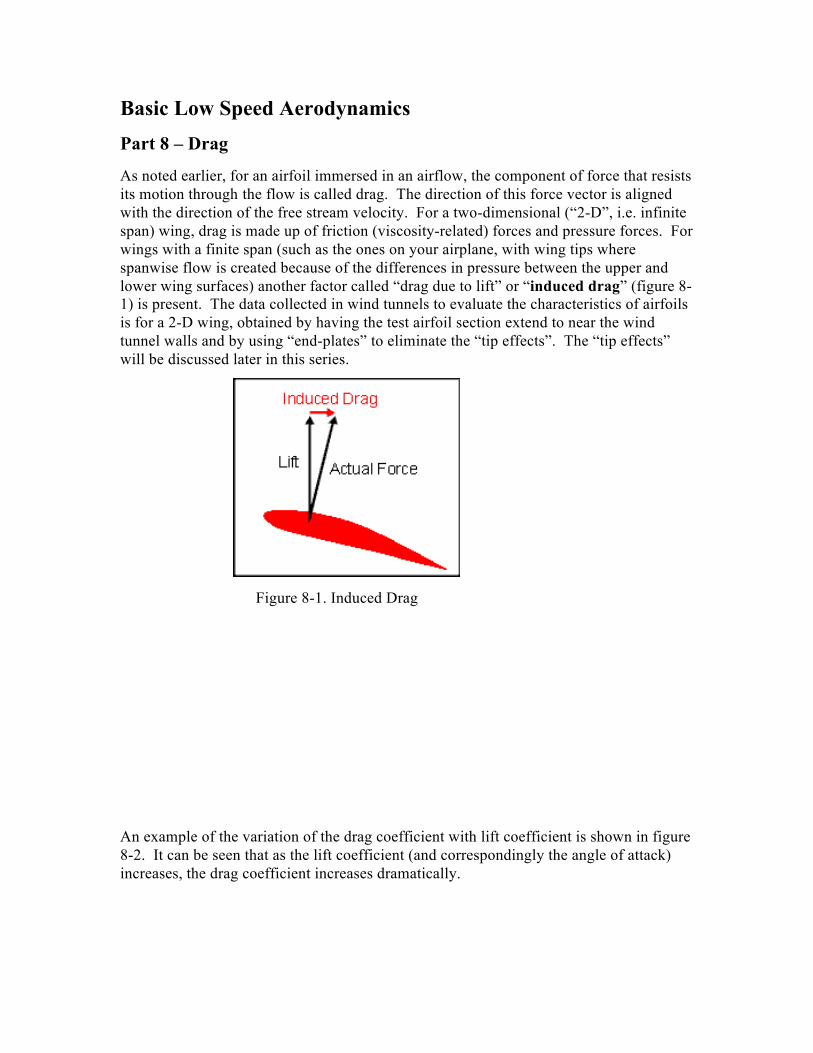
As noted earlier, for an airfoil immersed in an airflow, the component of force that resists its motion through the flow is called drag. The direction of this force vector is aligned with the direction of the free stream velocity. For a two-dimensional (“2-D”, i.e. infinite span) wing, drag is made up of friction (viscosity-related) forces and pressure forces. For wings with a finite span (such as the ones on your airplane, with wing tips where spanwise flow is created because of the differences in pressure between the upper and lower wing surfaces) another factor called “drag due to lift” or “induced drag” (figure 8-1) is present. The data collected in wind tunnels to evaluate the characteristics of airfoils is for a 2-D wing, obtained by having the test airfoil section extend to near the wind tunnel walls and by using “end-plates” to eliminate the “tip effects”. The “tip effects” will be discussed later in this series. Figure 8-1. Induced Drag An example of the variation of the drag coefficient with lift coefficient is shown in figure 8-2. It can be seen that as the lift coefficient (and correspondingly the angle of attack) increases, the drag coefficient increases dramatically.

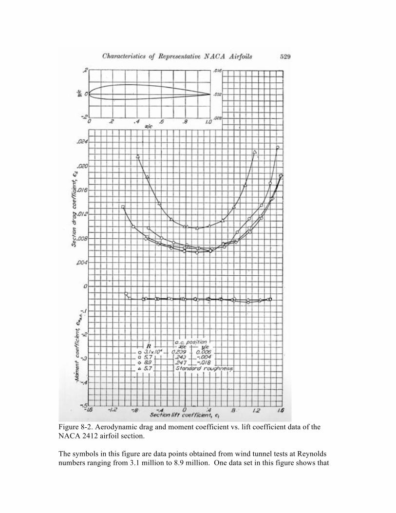
Figure 8-2. Aerodynamic drag and moment coefficient vs. lift coefficient data of the NACA 2412 airfoil section. The symbols in this figure are data points obtained from wind tunnel tests at Reynolds numbers ranging from 3.1 million to 8.9 million. One data set in this figure shows that

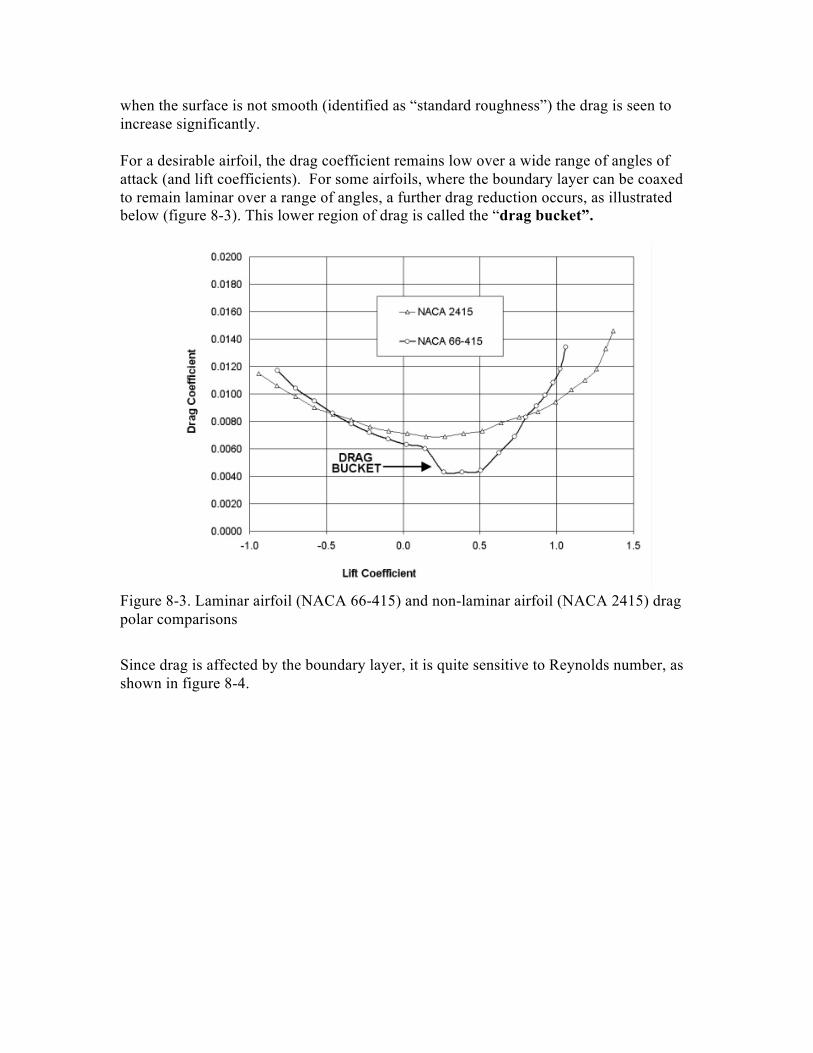
when the surface is not smooth (identified as “standard roughness”) the drag is seen to increase significantly. For a desirable airfoil, the drag coefficient remains low over a wide range of angles of attack (and lift coefficients). For some airfoils, where the boundary layer can be coaxed to remain laminar over a range of angles, a further drag reduction occurs, as illustrated below (figure 8-3). This lower region of drag is called the “drag bucket”.

Figure 8-3. Laminar airfoil (NACA 66-415) and non-laminar airfoil (NACA 2415) drag polar comparisons Since drag is affected by the boundary layer, it is quite sensitive to Reynolds number, as shown in figure 8-4.

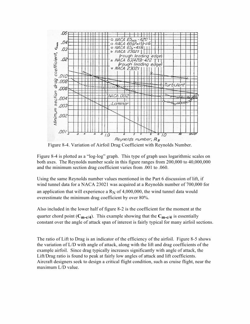
Figure 8-4. Variation of Airfoil Drag Coefficient with Reynolds Number. Figure 8-4 is plotted as a “log-log” graph. This type of graph uses logarithmic scales on both axes. The Reynolds number scale in this figure ranges from 200,000 to 40,000,000 and the minimum section drag coefficient varies from .001 to .060. Using the same Reynolds number values mentioned in the Part 6 discussion of lift, if wind tunnel data for a NACA 23021 was acquired at a Reynolds number of 700,000 for an application that will experience a RN of 4,000,000, the wind tunnel data would overestimate the minimum drag coefficient by over 80%. Also included in the lower half of figure 8-2 is the coefficient for the moment at the quarter chord point (Cm-c/4). This example showing that the Cm-c/4 is essentially constant over the angle of attack span of interest is fairly typical for many airfoil sections. The ratio of Lift to Drag is an indicator of the efficiency of the airfoil. Figure 8-5 shows the variation of L/D with angle of attack, along with the lift and drag coefficients of the example airfoil. Since drag typically increases significantly with angle of attack, the Lift/Drag ratio is found to peak at fairly low angles of attack and lift coefficients. Aircraft designers seek to design a critical flight condition, such as cruise flight, near the maximum L/D value.

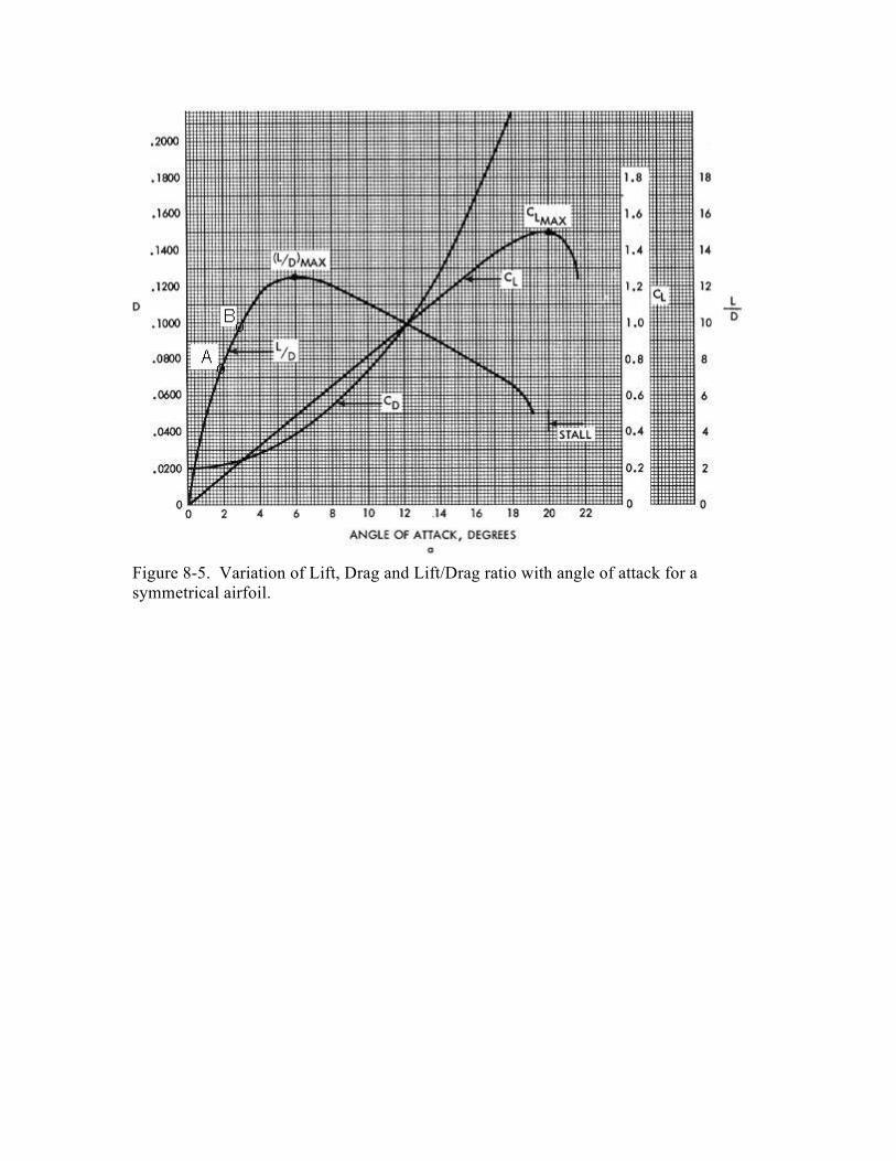
Figure 8-5. Variation of Lift, Drag and Lift/Drag ratio with angle of attack for a symmetrical airfoil.

Basic Low Speed Aerodynamics

Part 9 - Aircraft Drag

Drag is produced by a number of factors. When considering the drag of the entire aircraft, a building-block approach is taken. This section will discuss the principal components and the methods used to analyze total aircraft drag. First, a few more terms will be introduced. Parasite Drag (DP) is, the resistance force developed by the movement of a solid body through the air due to the geometry and surface characteristics of the body. This includes components called Form Drag (due to the body’s size and shape, vents and cooling flows, and protuberances (such as “blisters” and other surface irregularities)), Interference Drag (caused by vortices generated in the vicinity of a sharp angle intersection of two adjacent surfaces), and Skin Friction Drag (caused by the viscosity of the air resulting in friction along the body’s surface). Parasite drag can be expressed using a drag coefficient (CDP) that includes all of these components. DP = CDP(qSW)

q = Dynamic Pressure = ρV2/2, lb/ft2

and SW = Wing Area, ft2

With CD0 being the value of the minimum parasite drag coefficient at zero lift: DP 0 = CD0(qSW)

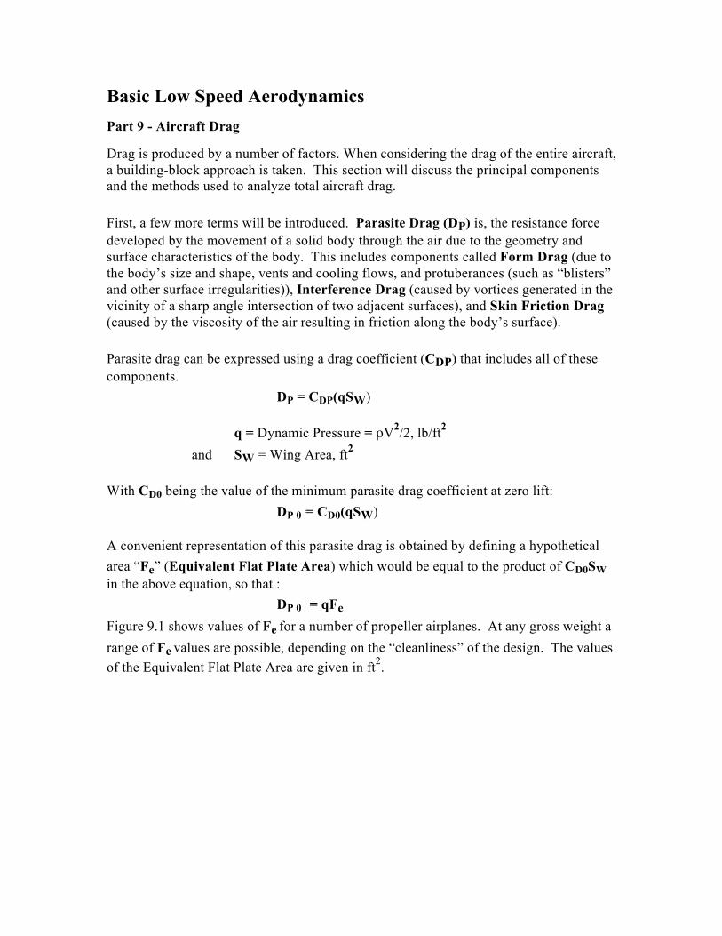
A convenient representation of this parasite drag is obtained by defining a hypothetical area “Fe” (Equivalent Flat Plate Area) which would be equal to the product of CD0SW in the above equation, so that : DP 0 = qFe

Figure 9.1 shows values of Fe for a number of propeller airplanes. At any gross weight a range of Fe values are possible, depending on the “cleanliness” of the design. The values of the Equivalent Flat Plate Area are given in ft2.

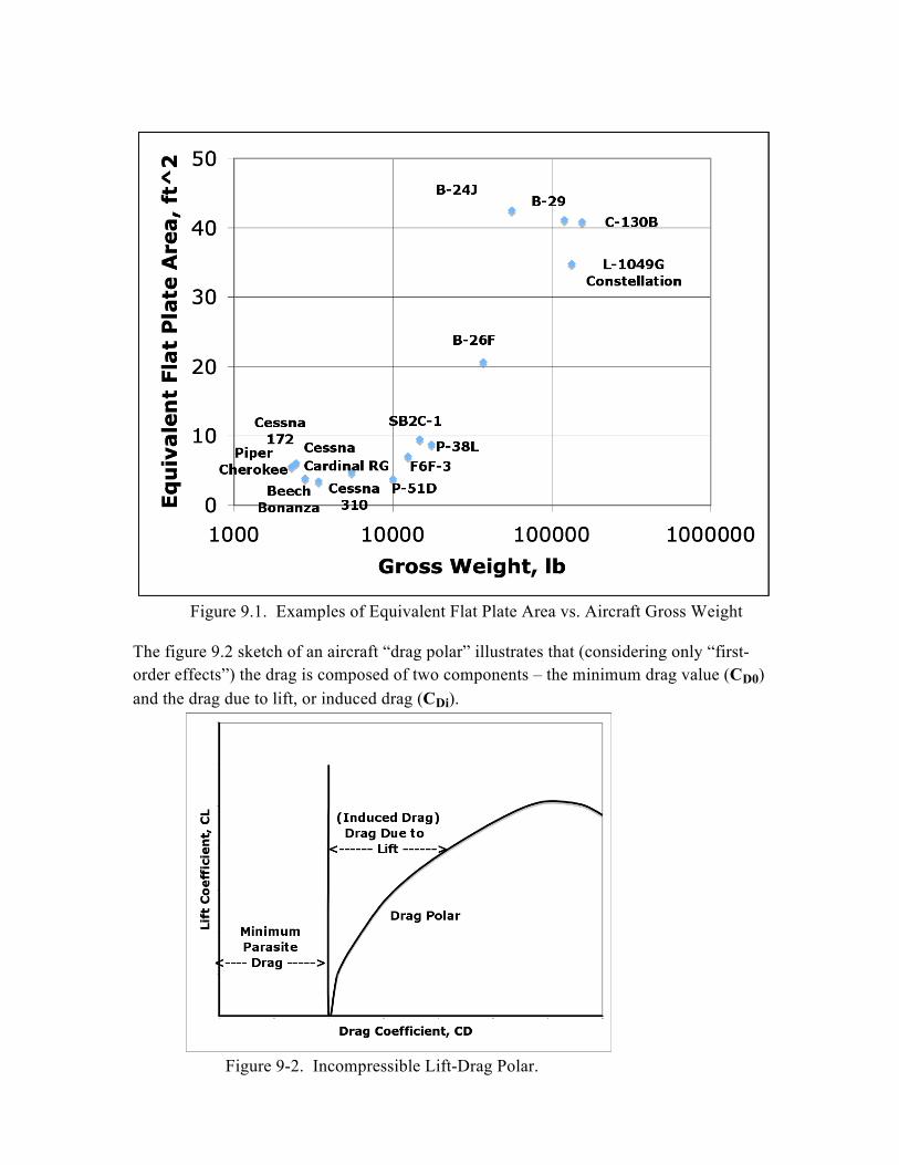
Figure 9.1. Examples of Equivalent Flat Plate Area vs. Aircraft Gross Weight The figure 9.2 sketch of an aircraft “drag polar” illustrates that (considering only “first-order effects”) the drag is composed of two components – the minimum drag value (CD0) and the drag due to lift, or induced drag (CDi).

Figure 9-2. Incompressible Lift-Drag Polar.

Analysis of the influence of the trailing vortices on the flow in the vicinity of a lifting wing, the following relationship for drag due to lift can be developed (in coefficient terms): CDi = CL

2/(πeAR) Or , in dimensional terms: Remembering that: L = CL qSw And solving for CL: CL = L/(qSw) The induced drag becomes: Di = CDi(qSw) = L2/(qSwπeAR)

Where: CDi = Induced Drag Coefficient, dimensionless Di = Induced Drag, lb q = Dynamic Pressure, lb/ft2 Sw = Wing area, ft2 L = Lift (or, in Steady Level Flight = Gross Weight (GW)), lb e = Wing Span (Oswald) Efficiency Factor, dimensionless AR = Wing Aspect Ratio = (Wing Span)2 /Sw, dimensionless π = Pi (mathematical constant 3.14159 ) The Oswald span efficiency factor (e, a value usually between 0.7 and 0.95) is related to the degree to which the wing tip vortices influence the level of induced drag. With respect to span efficiency, the most efficient shape is the elliptical planform as seen on the WWII Spitfire. The use of wing tip end-plates or winglets can reduce the adverse effect of the tip vortices on non-optimum wing shapes, thereby increasing the span efficiency factor and reducing the induced drag. Caution must be used when considering these approaches because they could also lead to an increase in form or interference drag that may offset the benefits. For a rectangular wing planform with: b = Wing Span, ft and - c = Wing Chord, ft the wing area is: Sw = bc the aspect ratio (defined as (Wing Span)2 /Sw) is: AR = b2/(bc) = b/c Substituting these terms in the induced drag equation, and assuming a steady, level 1-g flight condition where L = GW, the induced drag equation becomes: Di = (GW/b)2/(π q e)

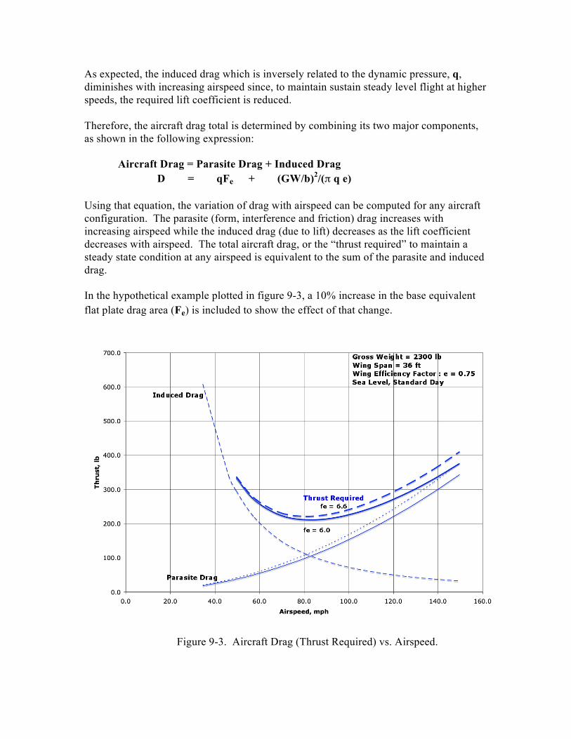
As expected, the induced drag which is inversely related to the dynamic pressure, q, diminishes with increasing airspeed since, to maintain sustain steady level flight at higher speeds, the required lift coefficient is reduced. Therefore, the aircraft drag total is determined by combining its two major components, as shown in the following expression: Aircraft Drag = Parasite Drag + Induced Drag D = qFe + (GW/b)2/(π q e) Using that equation, the variation of drag with airspeed can be computed for any aircraft configuration. The parasite (form, interference and friction) drag increases with increasing airspeed while the induced drag (due to lift) decreases as the lift coefficient decreases with airspeed. The total aircraft drag, or the “thrust required” to maintain a steady state condition at any airspeed is equivalent to the sum of the parasite and induced drag. In the hypothetical example plotted in figure 9-3, a 10% increase in the base equivalent flat plate drag area (Fe) is included to show the effect of that change.

Figure 9-3. Aircraft Drag (Thrust Required) vs. Airspeed.

Basic Low Speed Aerodynamics

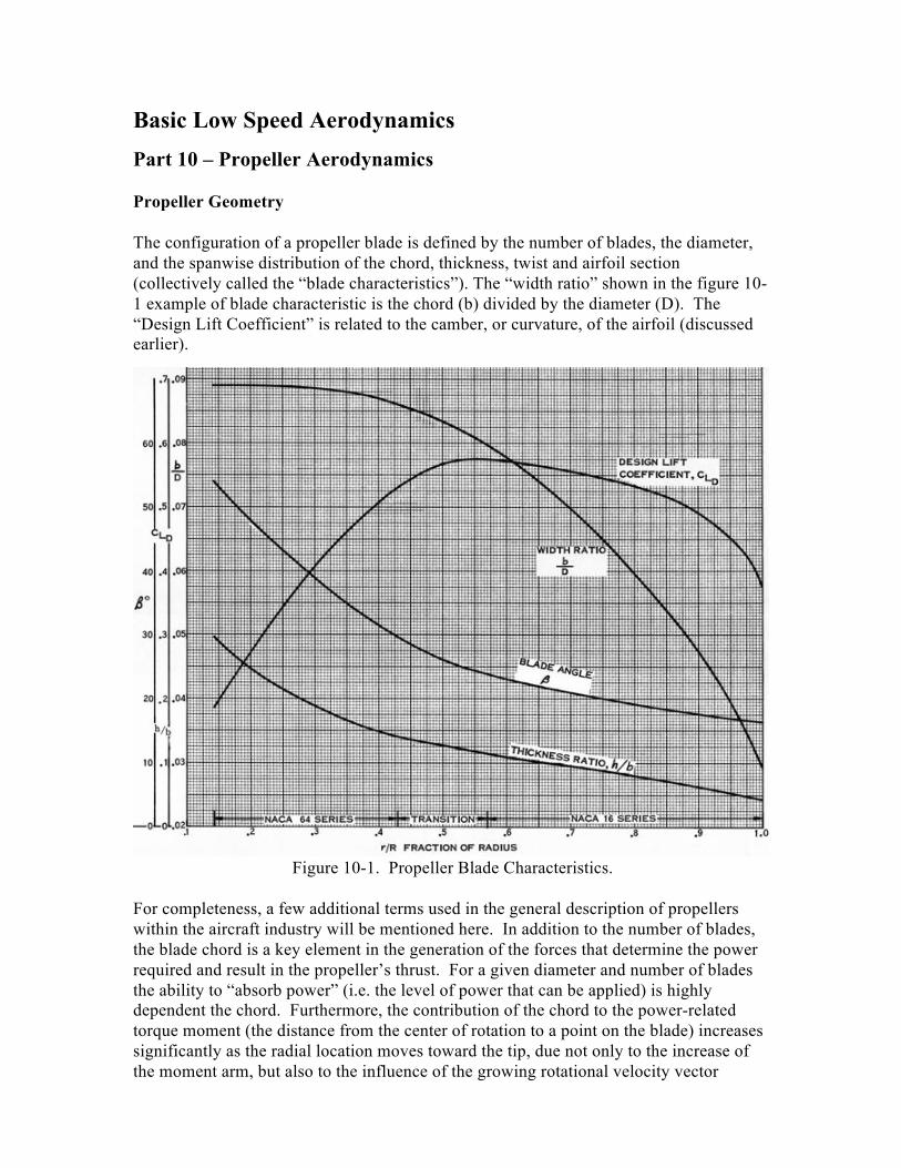
Part 10 – Propeller Aerodynamics Propeller Geometry The configuration of a propeller blade is defined by the number of blades, the diameter, and the spanwise distribution of the chord, thickness, twist and airfoil section (collectively called the “blade characteristics”). The “width ratio” shown in the figure 10-1 example of blade characteristic is the chord (b) divided by the diameter (D). The “Design Lift Coefficient” is related to the camber, or curvature, of the airfoil (discussed earlier).

Figure 10-1. Propeller Blade Characteristics. For completeness, a few additional terms used in the general description of propellers within the aircraft industry will be mentioned here. In addition to the number of blades, the blade chord is a key element in the generation of the forces that determine the power required and result in the propeller’s thrust. For a given diameter and number of blades the ability to “absorb power” (i.e. the level of power that can be applied) is highly dependent the chord. Furthermore, the contribution of the chord to the power-related torque moment (the distance from the center of rotation to a point on the blade) increases significantly as the radial location moves toward the tip, due not only to the increase of the moment arm, but also to the influence of the growing rotational velocity vector

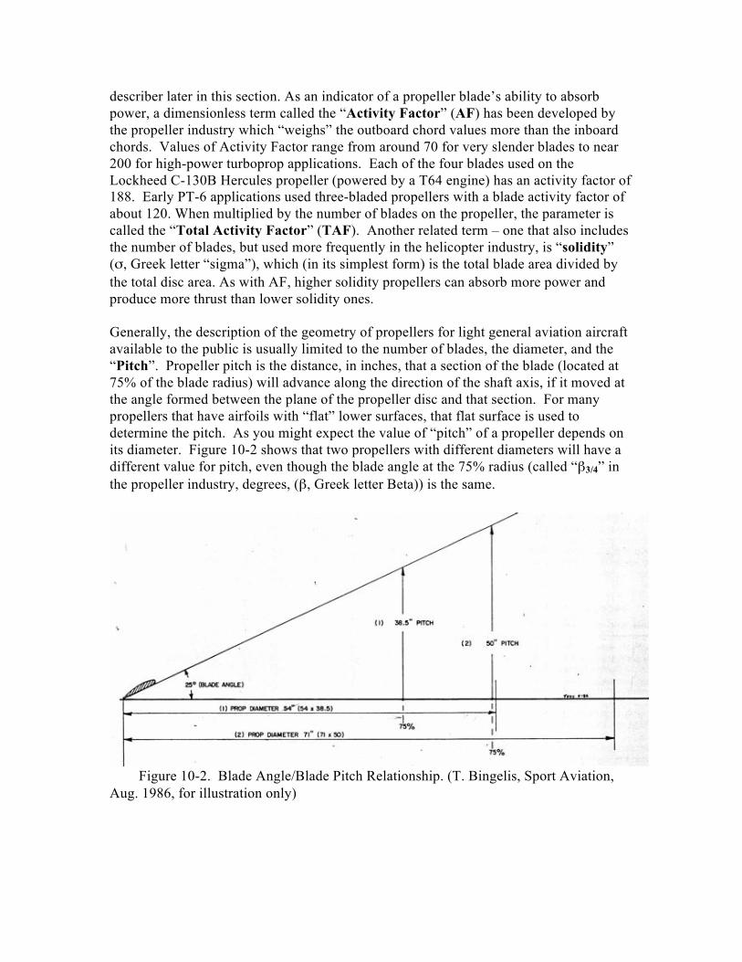
describer later in this section. As an indicator of a propeller blade’s ability to absorb power, a dimensionless term called the “Activity Factor” (AF) has been developed by the propeller industry which “weighs” the outboard chord values more than the inboard chords. Values of Activity Factor range from around 70 for very slender blades to near 200 for high-power turboprop applications. Each of the four blades used on the Lockheed C-130B Hercules propeller (powered by a T64 engine) has an activity factor of 188. Early PT-6 applications used three-bladed propellers with a blade activity factor of about 120. When multiplied by the number of blades on the propeller, the parameter is called the “Total Activity Factor” (TAF). Another related term – one that also includes the number of blades, but used more frequently in the helicopter industry, is “solidity” (σ, Greek letter “sigma”), which (in its simplest form) is the total blade area divided by the total disc area. As with AF, higher solidity propellers can absorb more power and produce more thrust than lower solidity ones. Generally, the description of the geometry of propellers for light general aviation aircraft available to the public is usually limited to the number of blades, the diameter, and the “Pitch”. Propeller pitch is the distance, in inches, that a section of the blade (located at 75% of the blade radius) will advance along the direction of the shaft axis, if it moved at the angle formed between the plane of the propeller disc and that section. For many propellers that have airfoils with “flat” lower surfaces, that flat surface is used to determine the pitch. As you might expect the value of “pitch” of a propeller depends on its diameter. Figure 10-2 shows that two propellers with different diameters will have a different value for pitch, even though the blade angle at the 75% radius (called “β3/4” in the propeller industry, degrees, (β, Greek letter Beta)) is the same.

Figure 10-2. Blade Angle/Blade Pitch Relationship. (T. Bingelis, Sport Aviation, Aug. 1986, for illustration only)

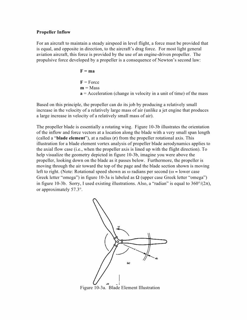
Propeller Inflow For an aircraft to maintain a steady airspeed in level flight, a force must be provided that is equal, and opposite in direction, to the aircraft’s drag force. For most light general aviation aircraft, this force is provided by the use of an engine-driven propeller. The propulsive force developed by a propeller is a consequence of Newton’s second law: F = ma F = Force m = Mass a = Acceleration (change in velocity in a unit of time) of the mass Based on this principle, the propeller can do its job by producing a relatively small increase in the velocity of a relatively large mass of air (unlike a jet engine that produces a large increase in velocity of a relatively small mass of air). The propeller blade is essentially a rotating wing. Figure 10-3b illustrates the orientation of the inflow and force vectors at a location along the blade with a very small span length (called a “blade element”), at a radius (r) from the propeller rotational axis. This illustration for a blade element vortex analysis of propeller blade aerodynamics applies to the axial flow case (i.e., when the propeller axis is lined up with the flight direction). To help visualize the geometry depicted in figure 10-3b, imagine you were above the propeller, looking down on the blade as it passes below. Furthermore, the propeller is moving through the air toward the top of the page and the blade section shown is moving left to right. (Note: Rotational speed shown as ω radians per second (ω = lower case Greek letter “omega”) in figure 10-3a is labeled as Ω (upper case Greek letter “omega”) in figure 10-3b. Sorry, I used existing illustrations. Also, a “radian” is equal to 360°/(2π), or approximately 57.3°.

Figure 10-3a. Blade Element Illustration

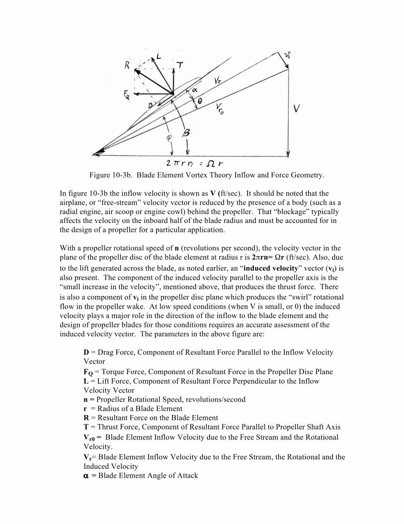
Figure 10-3b. Blade Element Vortex Theory Inflow and Force Geometry. In figure 10-3b the inflow velocity is shown as V (ft/sec). It should be noted that the airplane, or “free-stream” velocity vector is reduced by the presence of a body (such as a radial engine, air scoop or engine cowl) behind the propeller. That “blockage” typically affects the velocity on the inboard half of the blade radius and must be accounted for in the design of a propeller for a particular application. With a propeller rotational speed of n (revolutions per second), the velocity vector in the plane of the propeller disc of the blade element at radius r is 2πrn= Ωr (ft/sec). Also, due to the lift generated across the blade, as noted earlier, an “induced velocity” vector (vi) is also present. The component of the induced velocity parallel to the propeller axis is the “small increase in the velocity”, mentioned above, that produces the thrust force. There is also a component of vi in the propeller disc plane which produces the “swirl” rotational flow in the propeller wake. At low speed conditions (when V is small, or 0) the induced velocity plays a major role in the direction of the inflow to the blade element and the design of propeller blades for those conditions requires an accurate assessment of the induced velocity vector. The parameters in the above figure are:

D = Drag Force, Component of Resultant Force Parallel to the Inflow Velocity Vector FQ = Torque Force, Component of Resultant Force in the Propeller Disc Plane L = Lift Force, Component of Resultant Force Perpendicular to the Inflow Velocity Vector n = Propeller Rotational Speed, revolutions/second r = Radius of a Blade Element R = Resultant Force on the Blade Element T = Thrust Force, Component of Resultant Force Parallel to Propeller Shaft Axis Vr0 = Blade Element Inflow Velocity due to the Free Stream and the Rotational Velocity. Vr= Blade Element Inflow Velocity due to the Free Stream, the Rotational and the Induced Velocity α = Blade Element Angle of Attack

β = Blade Element Angle with respect to the Propeller Disc Plane Ω = Propeller Rotational Speed, radians/second ϕ = Inflow Angle

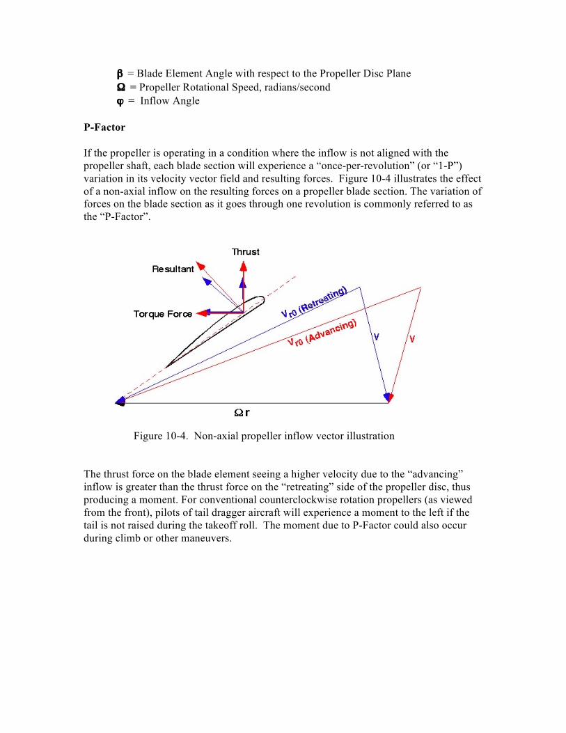
P-Factor If the propeller is operating in a condition where the inflow is not aligned with the propeller shaft, each blade section will experience a “once-per-revolution” (or “1-P”) variation in its velocity vector field and resulting forces. Figure 10-4 illustrates the effect of a non-axial inflow on the resulting forces on a propeller blade section. The variation of forces on the blade section as it goes through one revolution is commonly referred to as the “P-Factor”.

Figure 10-4. Non-axial propeller inflow vector illustration The thrust force on the blade element seeing a higher velocity due to the “advancing” inflow is greater than the thrust force on the “retreating” side of the propeller disc, thus producing a moment. For conventional counterclockwise rotation propellers (as viewed from the front), pilots of tail dragger aircraft will experience a moment to the left if the tail is not raised during the takeoff roll. The moment due to P-Factor could also occur during climb or other maneuvers.

Basic Low Speed Aerodynamics

Part 11 - Propeller Performance A rigorous propeller performance analysis ranks high among the most complex low speed aerodynamics tasks. Therefore, the discussion of this topic here will only look at the fundamental characteristics of the flow conditions at the propeller and will then describe the application of propeller performance data in the computation of aircraft performance. Background By the early 1930s practical solutions were developed for the challenging problem of analyzing the spanwise aerodynamic blade loads. The analytical methodology was based on computing the influence of trailing vortices in the propeller’s wake on the induced velocities at the propeller disc (called Wake Vortex Theory). These methods yielded results that compared well with experimental data for subsonic cruise propeller performance. The capability to accurately calculate low speed and static (0 airspeed) thrust, however, was not achieved until several decades later when improved propeller wake computational techniques coupled with high speed computers provided solutions that met the needs of Vertical Take-Off and Landing (VTOL) aircraft developers. For many general aviation propeller applications, less complex analytical methods for calculating propeller climb- and cruise-mode performance have been found to be satisfactory. These methods employ the momentum theory to estimate the local induced velocity and commonly utilize empirical adjustments to produce accurate results. Referring to figure 10-3b again, it can be seen that, while the free stream velocity component of the inflow (V) remains constant across the blade span (unless altered by the blockage effect of a fuselage or nacelle), the rotational component (Ωr) varies from “zero” at the propeller axis to a maximum value at the blade tip (called the “tip speed” = πnD, ft/sec). This variation alters the inflow angle ϕ across the span of the blade, resulting in the need to build a twist into the propeller blade to obtain the desired angles of attack at the design operating condition. Note that the proper design of a propeller blade is based on the angle ϕ and velocity Vr which include the induced inflow, instead of the less complex Vr0 determined only by the free stream and rotational velocity components. It should also be mentioned that although the aircraft velocity might be low enough to ensure that “incompressible” conditions exist for the airframe, portions of the propeller might be exposed to the problems associated with high subsonic Mach numbers. (The Mach number, named after Austrian physicist Ernst Mach, is the speed of an object moving through a fluid, divided by the speed of sound of the fluid). As the inflow to an airfoil increases above a Mach number of about 0.8, the drag increases significantly. That drag rise is referred to as “Mach drag divergence”. While seldom a issue within the airspeeds most EAA’ers see, high performance propeller aircraft such as racers and WWII fighters can encounter high Mach number inflow and compressibility effects not only near the blade tip, but, because of the high thickness found on inboard (near the

spinner) blade sections, penalties associated with compressibility drag rise can occur there as well.

Figure 11-1. Ernst Mach (1838-1916). The aerodynamic design of a propeller usually involves the evaluation of performance for at least two operation conditions and a determination of the relative importance of each condition. Typical design points for general aviation propellers would be a climb and a cruise condition. Because the different free stream inflow velocity, rotational speed and required thrust would result in a different optimum blade configuration for each condition, critical requirements must be identified in order to make the design selection. Performance at non-critical conditions, therefore will be compromised to some degree to obtain the performance required at the critical condition. The measure of the performance of a propeller in forward flight, its “efficiency” (η Greek letter “eta”), is determined by dividing the “output power” by the “input power” at a specific flight condition. For propeller applications (the helicopter industry uses a slightly different form of this term) the flight inflow condition is defined by the ratio of the free stream velocity (V), divided by an indicator of the rotational speed (nD). This parameter is called the “advance ratio” and, in propeller terminology is usually presented as the symbol “J”. For light general aviation aircraft, values of the non-dimensional J range from 0 to about 2, depending, of course, on the maximum velocity, propeller RPM and diameter. As can be seen from figure 10-3b, the advance ratio is related to the distance the tip moves in the direction of the propeller axis for each complete revolution. Restating the above relationships - Propeller Efficiency: η = Output Power/Input Power Advance Ratio: J = V/nD An example of the variation of propeller efficiency with advance ration for a fixed pitch propeller is shown in Figure 11-1. The β3/4 (blade angle at the 75% radius) for fixed pitch propellers is typical in the neighborhood of 15° to 20° which yields adequate climb and cruise performance for low-speed general aviation aircraft.

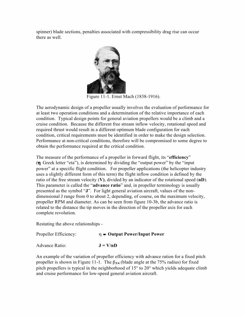
Figure 11-2. Propeller Efficiency Variation with Advance Ratio for a Fixed Pitch McCauley 7557 Propeller. The efficiency is seen to increase with advance ratio up to a point, after which it experiences a rapid decrease, eventually reaching an advance ratio where efficiency is zero. This may be crudely described first by noting that the thrust is related to lift and drag is related to power, and then considering the variation of the lift and drag coefficients for an airfoil (see parts 7 and 8) as the angle of attack diminishes (with increasing airspeed, or advance ratio – refer to figure 10-3b). If we start at a below-stall high angle of attack, the lift/drag ratio for the airfoil will increase as α is decreased, until a maximum L/D is reached. Further reduction in α results in a decrease of the L/D, eventually reaching a zero lift angle.

Basic Low Speed Aerodynamics Part 12 - Propeller Aircraft Available Thrust, Maximum Airspeed Nondimensional thrust and power coefficients have been defined that are used to describe the performance of a propeller, much like the lift and drag coefficients are used to represent the performance of an airfoil section. The expressions for propeller thrust and power coefficients are: T = CT ρn2D4 = CT ρ(N/60)2D4 P = CP ρn3D5 = CP ρ(N/60)3D5

Where: T = Thrust, lb P = Power, ft-lb/sec CT = Propeller Thrust Coefficient, nondimensional CP = Propeller Power Coefficient, nondimensional D = Diameter, ft n = Rotational speed, revolutions/sec N = Rotational speed, revolutions/min = n•60 ρ = Air density, lb-sec2/ft4 Since one unit of horsepower is defined as 550 ft-lb/sec, the power term becomes: HP = CP ρn3D5/550 Also, using the definition of power as work per unit time, and the definition of work is force * distance, we can write the following expressions: Power = Work/time Power = (Force * Distance)/time or- Power = Force * (Distance/time) Remembering from high school physics that Distance/time = Velocity, and labeling the Force as Thrust (i.e. the “output force” of the propeller), we can state that the power output of a propeller is: Output Power = Thrust * Velocity or- Output Horsepower = Thrust * Velocity / 550 Returning to the definition of propeller efficiency (η = Output Power/Input Power), we can now write: η = Thrust * Velocity / (550 SHP) = TAvail *V/(550*SHP) where: TAvail = Thrust Available (Output), lb V = Free Stream Velocity, ft/sec SHP = Horsepower input to the propeller shaft

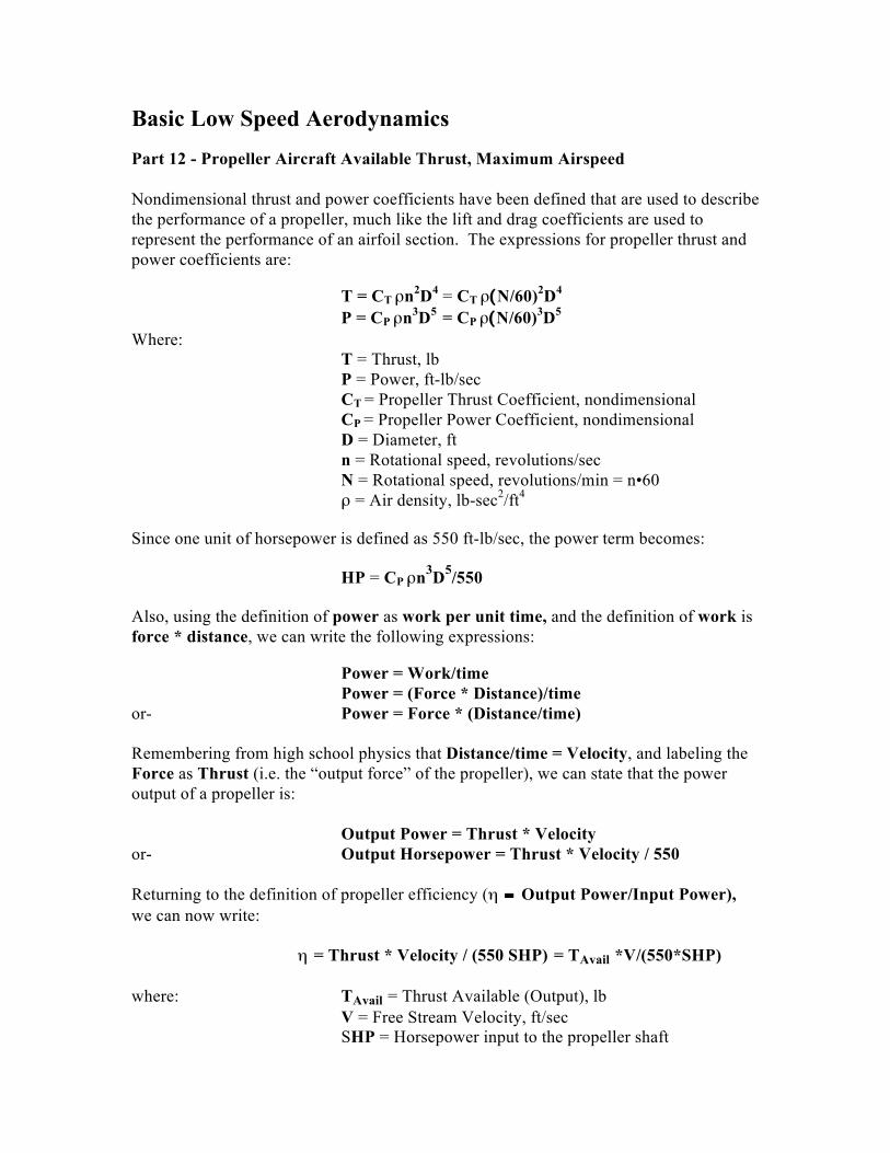
In coefficient form, using the above relationships, propeller efficiency becomes: η = J (CT /CP) Now solving for thrust from the above efficiency equation, we get: TAvail = η∗550*SHP/V For velocity expressed in miles per hour, the available thrust can be calculated by: TAvail = η∗375*SHP/Vmph It was noted earlier that SHP is the horsepower input to the propeller shaft. For direct drive systems, this value is the engine output horsepower with accessory power subtracted. For drive systems that use a gearbox or other speed reduction devices, the power loss due to that element must also be accounted for. Referring to figure 11-2, it can be seen that a fixed pitch propeller cannot provide “optimum” performance (i.e. high efficiencies) over a wide range of flight conditions – this is why, for a fixed pitch prop, you will select either a “climb” propeller or a “cruise” propeller, and why we will now look at the performance of a variable pitch propeller. Just remember that, for fixed pitch propellers, while the pitch (blade angle) must be high enough to offer good cruising performance, it must be low enough to achieve acceptable takeoff and climb characteristics. Figure 12-1 shows the variation of efficiency with advance ratio for a range of blade angles from 15° to 45°. It can be seen that the maximum efficiency at the higher blade angles occurs at higher advance ratios. Variable pitch, therefore, allows the propeller to operate at a blade angle that is appropriate for the flight condition, from the low β3/4 required for takeoff to a high β3/4 for the maximum velocity condition.

Figure 12-1. Propeller Efficiency as a Function of Advance Ratio and Blade Angle (McCormick, 1979).

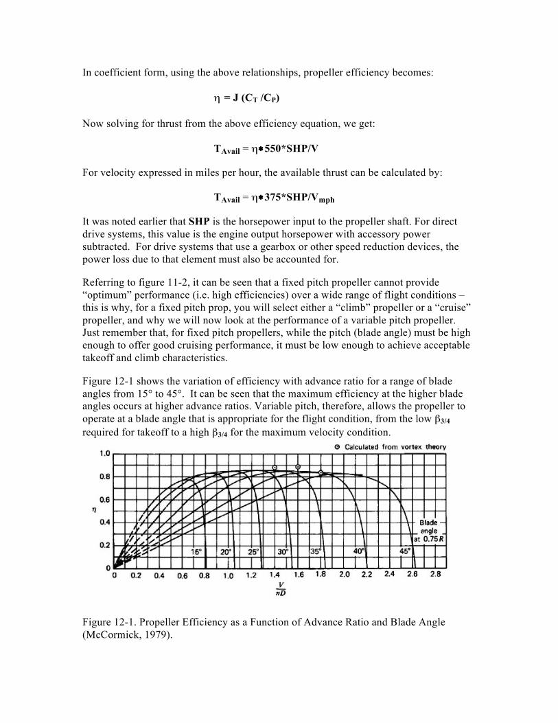
Maximum Aircraft Airspeed Returning to the fixed pitch propeller case, it is now possible to compute the variation of available thrust with airspeed by using the figure 11-1 efficiency values and the preceding thrust equation. Figure 12-2 shows, for this hypothetical case, the available thrust plotted with the previously calculated aircraft drag (or required thrust, figure 9-3). For this calculation the power and engine RPM are assumed to be constant. To show the sensitivity to power changes, the effect of a 10% increase in power is included. The intersection of the available (red) and required (blue) thrust lines at the high-speed end of the plot establishes the aircraft’s maximum achievable airspeed at the altitude and temperature conditions examined. Note that the selection of a “climb”- oriented prop would shift the Thrust Available (red) lines to the left. A “cruise” prop would shift the Thrust Available lines to the right.

Figure 12-2. Aircraft Thrust Required and Thrust Available vs. Airspeed It should be pointed out that the data presented in figure 12-3 is conventionally shown in terms of power, expressed as Thrust Horsepower, versus airspeed. (I used thrust in this example because it is a familiar term, perhaps easier to comprehend than thrust horsepower). The following expressions are used to compute Thrust Horsepower: Thrust Horsepower Required = THPReq = TReq*V / 550 Thrust Horsepower Available = THPAvail = η*SHP TReq = Thrust Required = Drag, lb

V = Free Stream Velocity, ft/sec SHP = Horsepower input to the propeller shaft. η = Propeller Efficiency In addition to the determination of maximum speed, figure 12-2 provides other information about the aircraft’s performance. The “excess thrust”, or the amount that the available thrust exceeds the required thrust at any airspeed, will be seen to be the force that allows the aircraft to climb. Also, as airspeed is reduced from a cruise condition, the lift coefficient necessary to support the aircraft increases until the maximum lift coefficient is reached. The airspeed at which CLmax occurs is the stall speed discussed in part 7. Below that airspeed, steady level flight can not be maintained.

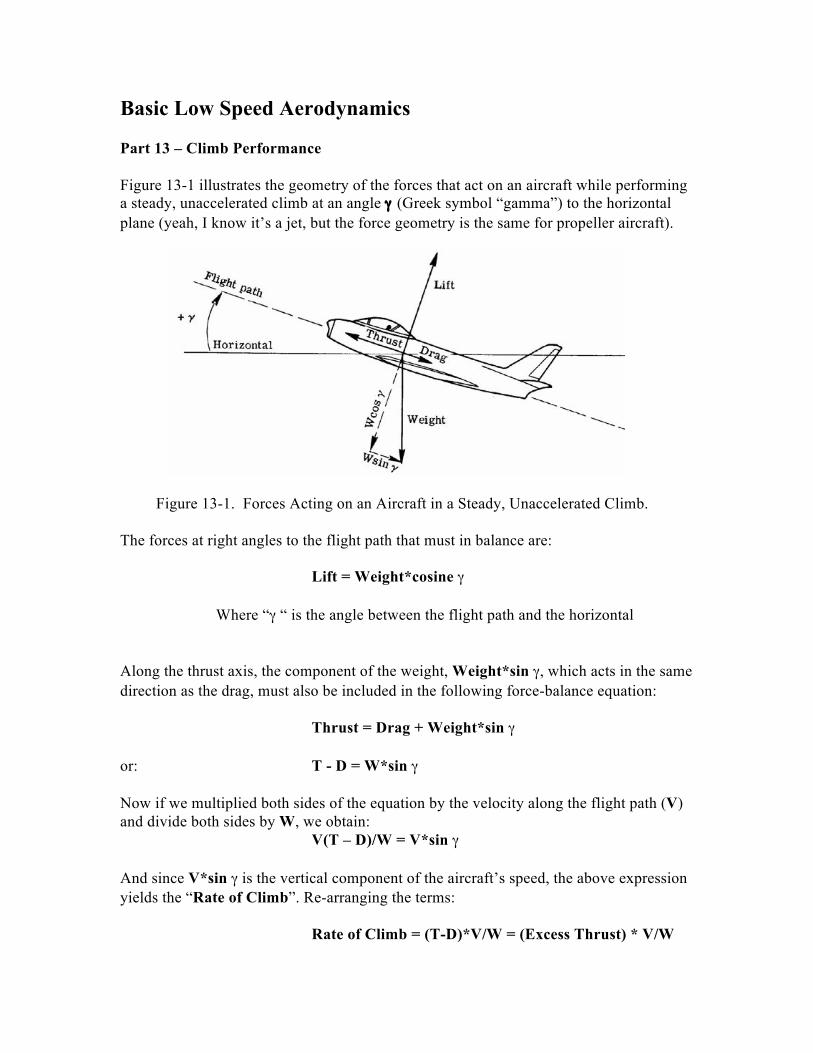
Basic Low Speed Aerodynamics Part 13 – Climb Performance Figure 13-1 illustrates the geometry of the forces that act on an aircraft while performing a steady, unaccelerated climb at an angle γ (Greek symbol “gamma”) to the horizontal plane (yeah, I know it’s a jet, but the force geometry is the same for propeller aircraft).

Figure 13-1. Forces Acting on an Aircraft in a Steady, Unaccelerated Climb. The forces at right angles to the flight path that must in balance are:

Lift = Weight*cosine γ Where “γ “ is the angle between the flight path and the horizontal

Along the thrust axis, the component of the weight, Weight*sin γ, which acts in the same direction as the drag, must also be included in the following force-balance equation:

Thrust = Drag + Weight*sin γ or: T - D = W*sin γ Now if we multiplied both sides of the equation by the velocity along the flight path (V) and divide both sides by W, we obtain: V(T – D)/W = V*sin γ And since V*sin γ is the vertical component of the aircraft’s speed, the above expression yields the “Rate of Climb”. Re-arranging the terms: Rate of Climb = (T-D)*V/W = (Excess Thrust) * V/W

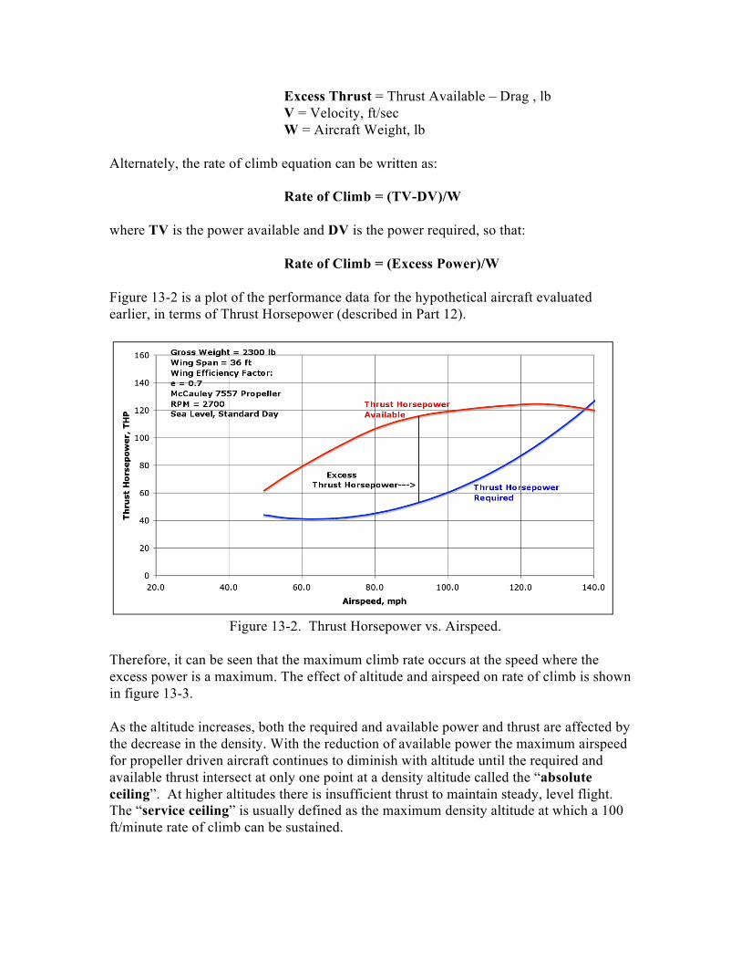
Excess Thrust = Thrust Available – Drag , lb V = Velocity, ft/sec W = Aircraft Weight, lb Alternately, the rate of climb equation can be written as: Rate of Climb = (TV-DV)/W where TV is the power available and DV is the power required, so that: Rate of Climb = (Excess Power)/W Figure 13-2 is a plot of the performance data for the hypothetical aircraft evaluated earlier, in terms of Thrust Horsepower (described in Part 12).

Figure 13-2. Thrust Horsepower vs. Airspeed. Therefore, it can be seen that the maximum climb rate occurs at the speed where the excess power is a maximum. The effect of altitude and airspeed on rate of climb is shown in figure 13-3. As the altitude increases, both the required and available power and thrust are affected by the decrease in the density. With the reduction of available power the maximum airspeed for propeller driven aircraft continues to diminish with altitude until the required and available thrust intersect at only one point at a density altitude called the “absolute ceiling”. At higher altitudes there is insufficient thrust to maintain steady, level flight. The “service ceiling” is usually defined as the maximum density altitude at which a 100 ft/minute rate of climb can be sustained.

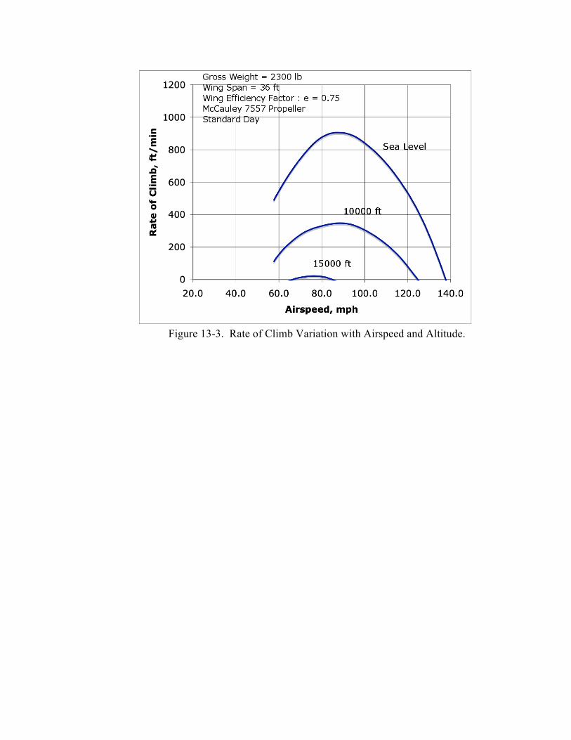
Figure 13-3. Rate of Climb Variation with Airspeed and Altitude.

Basic Low Speed Aerodynamics Part 14 – Range

To determine the maximum endurance and range of a propeller driven aircraft, the rate of fuel consumption as a function of power must be known. Specific fuel consumption (sfc) is a measure of the fuel flow rate per unit power, and is commonly dimensionally expressed as lb/(HP-Hour). Values for sfc for light aircraft engines are in the vicinity of 0.3 to 0.45 for the normal operating range of power. The change in the weight of the aircraft as fuel is burnt off (ΔW) for an increment of time (Δ t) can be expressed as: ΔW = sfc*P*Δ t where sfc = Specific Fuel Consumption, lb/((ft-lb/sec)sec) P = Power, ft-lb/sec ( = HP*550) Δ t = Time increment, seconds Solving for the time increment: Δ t = ΔW/(sfc*P) Remembering that velocity is defined as the change in distance for a given increment in time (V = Δs/Δ t, where s is the term for distance), we can write: Δ t = Δs/V = ΔW/(sfc*P) or Δs = V*ΔW/(sfc*P) In Part 12 it was shown that for steady level flight the power required is D*V, and the propeller output power (P) is equal to the engine output power (Pengine ) multiplied by the propeller efficiency, PAvail = η*Pengine , so that Pengine = P/η = D*V/η, and the equation becomes: Δs = V*ΔW/(sfc*D*V/η) = η ΔW/(sfc*D) Multiplying the right side of the equation by W/W: Δs = ηW ΔW/(sfc*D*W) Since, for level flight L = W the equation can be rewritten as: Δs = (η/sfc)(L/D) (ΔW/W) Now, if η, sfc, and aircraft L/D (which equals CL/CD) are assumed to have constant average values throughout the flight the total distance may be calculated from the above equation. The solution to the integral equation is called the Breguet Range formula (originally developed by Louis Charles Breguet, 1880-1955, a French airplane engineer).

Figure 14-1. Louis Charles Breguet.

Breguet Range Equation: R = 375 (η/sfc) (CL/CD) ln(W0/W1) η = Propeller Efficiency, dimensionless sfc = Specific Fuel Consumption, lb/(HP-hr) CL/CD = Aircraft Lift/Drag Ratio, dimensionless R = Range, statute miles W0 = Initial Aircraft Gross Weight, lb

W1 = Final Aircraft Gross Weight = (W0 – (Fuel & Oil Consumed)), lb ln (W0/W1) = Natural Logarithm (mathematical function) of (W0/W1) Therefore, to obtain the maximum range possible the aircraft should be operated at a condition that provides the best combination of the maximum Lift/Drag ratio, the highest achievable propeller efficiency and the lowest sfc throughout the flight. Furthermore, the fuel load must be as large as possible in comparison to the empty weight. For the remainder of this example, the sfc will be considered to be constant. However, the L/D ratio and the propeller efficiency do vary with airspeed. Also, this section will not consider the effect of the climb and descent on the achievable range. The variation of the aircraft Lift/Drag ratio with airspeed is shown in figure 14-2 for a 10000 ft standard day condition. The peak L/D in this case occurs at about 110 mph.

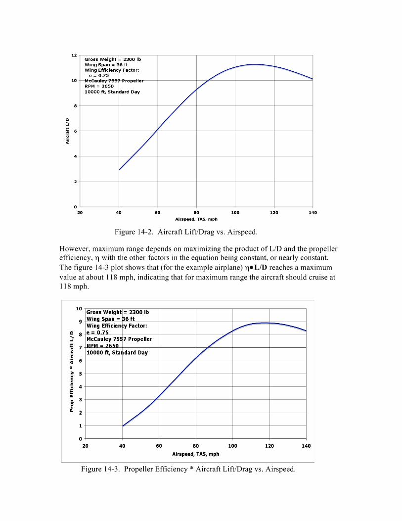
Figure 14-2. Aircraft Lift/Drag vs. Airspeed. However, maximum range depends on maximizing the product of L/D and the propeller efficiency, η with the other factors in the equation being constant, or nearly constant. The figure 14-3 plot shows that (for the example airplane) η∗L/D reaches a maximum value at about 118 mph, indicating that for maximum range the aircraft should cruise at 118 mph.

Figure 14-3. Propeller Efficiency * Aircraft Lift/Drag vs. Airspeed.