
Basic Concepts of Digital Signal Processing Basic Concepts of Digital Signal Processing B-IT, IPEC...
524
Basic Concepts of Digital Signal Processing Prof. Dr. Michael Clausen, Dr. Meinard M¨ uller Institut f¨ ur Informatik III R¨ omerstraße 164 Rheinische Friedrich-Wilhelms-Universit¨ at Bonn {clausen, meinard}@cs.uni-bonn.de Summer School 2003 International Program of Excellence (IPEC) Bonn-Aachen International Center for Information Technology (B-IT)
Transcript of Basic Concepts of Digital Signal Processing Basic Concepts of Digital Signal Processing B-IT, IPEC...

Basic Concepts of Digital Signal Processing
Prof. Dr. Michael Clausen, Dr. Meinard Muller
Institut fur Informatik III
Romerstraße 164
Rheinische Friedrich-Wilhelms-Universitat Bonn
clausen, [email protected]
Summer School 2003
International Program of Excellence (IPEC)
Bonn-Aachen International Center for Information Technology (B-IT)

Clausen/Muller: Basic Concepts of Digital Signal Processing B-IT, IPEC
Preface
These slides were used in the lecture “Basic Concepts of Digital Signal Processing” held
within the Summer School 2003 of the International Programme of Excellence (IPEC) of
the Bonn-Aachen International Center for Information Technology (B-IT). We hope that
these slides give the students a rough guideline and a summary of the main concepts
covered by the lecture. However, these slides are not meant to be self-contained or
complete. Further details, illustrations, proofs, and explanations are given in the lecture.
The authors would be grateful for any comments and suggestions for improvement.
Bonn, August 2003Michael Clausen
Meinard Muller
§ -1 2

Clausen/Muller: Basic Concepts of Digital Signal Processing B-IT, IPEC
Contents
Preface
1 Signals and Signal Spaces
1.1 Motivation and Examples
1.2 Signals
1.2.1 Continuous-time (CT) signals
1.2.2 Discrete-time (DT) signals
1.3 Signal Spaces
1.3.1 Banach Spaces and Hilbert Spaces
1.3.2 Lebesgue Space `p(Z) for DT-Signals
1.3.3 Lebesgue Space Lp(R) for CT-Signals
1.3.4 Lebesgue Space Lp([0, 1])
§ -1 3

Clausen/Muller: Basic Concepts of Digital Signal Processing B-IT, IPEC
2 Fourier Transform
2.1 Fourier Series for Periodic CT-Signals
2.2 Fourier Integral for non-periodic CT-Signals
2.3 Fourier Transform for DT-Signals
2.4 Discrete Fourier Transform
3 Systems and Filters
3.1 Linear Filter and LTI-Systems
3.2 Convolution Filter
3.3 Frequency Response
3.4 z-Transform and Transfer Function
3.5 Convolution for CT-Signals
3.6 Summary and Examples
3.6.1 Haar filter
3.6.2 Averaging Filter
§ -1 4

Clausen/Muller: Basic Concepts of Digital Signal Processing B-IT, IPEC
4 Sampling and Aliasing
4.1 Sampling
4.2 Shannon Sampling Theorem
4.3 Aliasing
4.4 Down- und Upsampling
4.4.1 Sampling operators in the z-domain
4.4.2 Sampling operators in the Fourier domain
5 FIR Filters
5.1 Causality and its Implications
5.2 The Ideal Lowpass Filter
5.3 Characteristics of Practical Frequency-Selective Filters
5.4 Linear-Phase FIR Filters
5.5 Design of Linear-Phase FIR Filters Using Windows
5.5.1 Windowing with the Box-Function
5.5.2 Windowing with the Hamming Window
5.6 Bandpass Filter from Lowpass Filter
§ -1 5

Clausen/Muller: Basic Concepts of Digital Signal Processing B-IT, IPEC
6 Windowed Fourier Transform (WFT)
6.1 Defintion of the WFT
6.2 Examples
6.2.1 Window Functions
6.2.2 WFT of a Chirp Signal
6.2.3 WFT in Dependence of the Window Size
6.3 Time-Frequency Localization of the WFT
6.3.1 Heisenberg Uncertainty Principle
6.3.2 Information Cells
6.3.3 Reconstruction of the Signal from its WFT
6.4 Discrete Version of the WFT
6.5 Drawback of the WFT
7 Continuous Wavelet Transform (CWT)
7.1 Definition of the CWT
7.2 Examples of Wavelets
§ -1 6

Clausen/Muller: Basic Concepts of Digital Signal Processing B-IT, IPEC
7.3 Time-frequency localization of the CWT
7.4 Examples of some CWTs
7.4.1 CWT of some Chirp Signal
7.4.2 CWT of Sines with Impulses.
7.4.3 Reconstruction of the Signal from its CWT
7.5 Discrete Version of the CWT
7.5.1 CWT-Adapted Grid
7.5.2 Wavelet Frames
8 Multiresolution Analysis (MRA) and Wavelet Transform
8.1 Multiresolution Analysis (MRA)
8.1.1 Motivating Analogy
8.1.2 Definition of the MRA
8.2 MRA und Wavelets
8.2.1 Filter Coefficients and Scaling Equation
8.2.2 Filter Coefficients and Wavelets
8.2.3 Fast Wavelet Algorithms
§ -1 7
Clausen/Muller: Basic Concepts of Digital Signal Processing B-IT, IPEC
8.2.4 Fast Discrete Wavelet Transform (FDWT)
8.2.5 Fast Discrete Wavelet Reconstruction (FIDWT)
8.2.6 Complexity of the FDWT and FIDWT
8.2.7 Discretization step in the DWT
8.2.8 Pm, Qm and Wavelet Coefficients
8.3 Example: Haar-MRA
9 DWT-Based Applications
9.1 DWT-Based Denoising
9.1.1 White Noise
9.1.2 Thresholding
9.1.3 Choice of the Threshold
9.1.4 Algorithm for Denoising
9.1.5 Examples for Denoising
9.1.6 Problems and Remarks
9.2 DWT-Based Compression
§ -1 8

Clausen/Muller: Basic Concepts of Digital Signal Processing B-IT, IPEC
10 The Two-Dimensional (2D) Case
10.1 2D Fourier Transform
10.2 2D Fourier Transform
10.2.1 2D Fourier Transform for CT-Signals
10.2.2 2D Fourier Transform for DT-Signals
10.2.3 2D z-Transform
10.3 Sampling and Aliasing in 2D
10.4 2D MRA and Wavelets
Literature
§ -1 9

Clausen/Muller: Basic Concepts of Digital Signal Processing B-IT, IPEC
Chapter 1: Signals and Signal Spaces
1.1 Motivation and Examples
In their classical book “Digital Signal Processing.” [Oppenheim/Schafer] the authors give
the following characterization of a signal.
A signal can be defined as a function that conveys information, generally about the
state of behavior of a physical system. Although signals can be represented in many
ways, in all cases the information is contained in a pattern of variations of some
form. For example, the signal may take the form of a pattern of time variations or a
spatially varying pattern. Signals are represented mathematically as functions of one
or more independent variables. For example, a speech signal would be represented
mathematically as a function of time and a picture would be represented as a brightness
function of two spatial variables.
§ 1 10

Clausen/Muller: Basic Concepts of Digital Signal Processing B-IT, IPEC
Signals include, for example,
• the sound of a piano as a signal represented by the amplitude of sound with respect to
time,
• the distribution of light on a screen, or
• the light falling on a point on a surface or in space.
We first consider the case of a music signal. From a physical point of view, the musician,
by means of his voice or instrument, generates an audio signal. This audio signal has the
form of a sound wave emerging at its source and spreading through the air. Graphically,
such an audio signal may be represented by its waveform which depicts the amplitude of
the air pressure over the time:
§ 1 11

Clausen/Muller: Basic Concepts of Digital Signal Processing B-IT, IPEC
Figure 1: Beginning of the Aria con Variazioni by J. S. Bach, BWV 988.
0 0.5 1 1.5 2 2.5 3 3.5
x 105
−0.1
−0.05
0
0.05
0.1
0.15
Figure 2: Waveform representation of an Aria interpretation of Fig. 1
§ 1 12

Clausen/Muller: Basic Concepts of Digital Signal Processing B-IT, IPEC
In case of a digital image, the signal may be represented as a matrix with entries in the
range [0 : 255]. Here each entry of the matrix represents a pixel and the value of the
entry encodes the gray level of the pixel.
Figure 3: Signal represented as 256 × 256 matrix over [0 : 255].
§ 1 13

Clausen/Muller: Basic Concepts of Digital Signal Processing B-IT, IPEC
From a mathematical point of view a signal is just a function. Basically there are two
different kinds of signals:
(1) continuous-time (CT) (or analog) signals
(2) discrete-time (DT) signals, also called discrete or sampled signals
For example, a physical sound wave can be thought of as a CT signal. However, a
computer can only store a finite set of numbers and (usually) can only compute with
finite precision. Therefore, in computer-based signal processing a continuous-time signal is
transformed into some discrete signal where the signal is stored as a collection of samples.
This transformation is also known as sampling. The discrete signal is only defined at
particular, discrete locations.
§ 1 14

Clausen/Muller: Basic Concepts of Digital Signal Processing B-IT, IPEC
Figure 4: Example for sampling.
Digital signal processing involves the creation of digital signals from continuous-time
signals. However, by sampling one looses in general information about the signal. The
side effects caused by the discrete representation of some continuous signal are known as
aliasing. In order to understand these side effects and the connection of the continuous
and discrete world we need a thorough mathematical modeling of the concepts involved.
In this chapter we start with the definition of signals and signal spaces.
§ 1 15

Clausen/Muller: Basic Concepts of Digital Signal Processing B-IT, IPEC
1.2 Signals
1.2.1 Continuous-time (CT) signals
Depending on the nature of the signal, a continuous-time (CT) signal can be mathematically
modeled as a
• one-dimensional real-valued function f : R → R
• one-dimensional complex-valued function f : R → C
For example, an audio signal may be represented by a function f : R → R, where the
domain R represents the time axis and the range R the amplitude of the sound wave.
Complex-valued functions generalize the concept of real-valued functions.
Why complex-valued functions? ; Fourier transform
§ 1 16

Clausen/Muller: Basic Concepts of Digital Signal Processing B-IT, IPEC
A signal, such as an image, can be modeled as a
• two-dimensional real-valued function f : R2 → R
• two-dimensional complex-valued function f : R2 → C
Here the domain R2 represents the two dimensional space (two spatial coordinates) and
the range R the gray level or color value.
In general, a signal is a parametric function of any number of input dimension n ∈ N and
output dimensions m ∈ N:
• n-dimensional R-vector-valued function f : Rn → R
m
• n-dimensional C-vector-valued function f : Rn → C
m
For example, a 3D-scene could be modeled by a 3-dimensional domain R3 with three
spatial coordinates. Or a moving 3D-scene may by modeled by a 4-dimensional domain
R4 with three spatial coordinates and one time coordinate.
§ 1 17

Clausen/Muller: Basic Concepts of Digital Signal Processing B-IT, IPEC
Attention:
• A continuous-time signal need not to be continuous as a function!
• The term “continous-time” is unfortunate because it implies that the parameter of the
function is a time value. In fact, the parameter (or argument) may represent anything,
including time, space, or any “continuous parameter”. Hence continuous-parameter
would be a better expression. But the term “continous-time” is firmly established in
literature, so we will use it here.
In the following we concentrate on signals of the form f : R → C (audio signals) and
later generalize to the case f : R2 → C (images).
§ 1 18

Clausen/Muller: Basic Concepts of Digital Signal Processing B-IT, IPEC
Example 1.1. Let A, f be real numbers, then the function
y(t) = A sin(2πft)
defines a sine wave with amplitude A and frequency f . From a musical point of view, A
represents the volume and f the pitch of the signal.
Example 1.2. The continuous-time box function has value 1 within some interval of width
W ∈ R centered at t = 0, and is 0 outside:
bW (t) :=
1 if |t| ≤ W/2,
0 otherwise.
Note that this is a continuous-time signal which is not continuous as a function.
§ 1 19
Clausen/Muller: Basic Concepts of Digital Signal Processing B-IT, IPEC
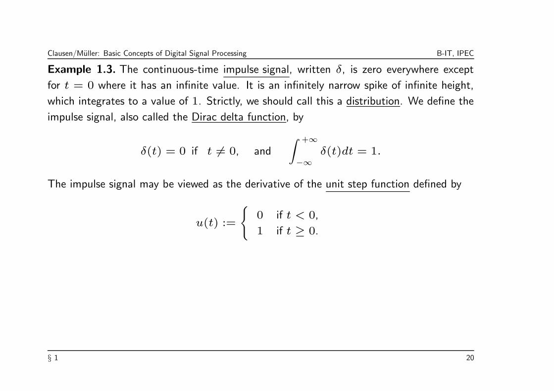
Example 1.3. The continuous-time impulse signal, written δ, is zero everywhere except
for t = 0 where it has an infinite value. It is an infinitely narrow spike of infinite height,
which integrates to a value of 1. Strictly, we should call this a distribution. We define the
impulse signal, also called the Dirac delta function, by
δ(t) = 0 if t 6= 0, and
∫ +∞
−∞δ(t)dt = 1.
The impulse signal may be viewed as the derivative of the unit step function defined by
u(t) :=
0 if t < 0,
1 if t ≥ 0.
§ 1 20

Clausen/Muller: Basic Concepts of Digital Signal Processing B-IT, IPEC
Example 1.4. A notational convenience is provided by the sinc (pronounced “sink”) signal
defined by:
sinc (t) :=
sinπtπt if t 6= 0,
1 if t = 0.
Prove as an exercise that this function is continuous. The sinc-function has a number of
remarkable properties which will play a crucial role in later chapters.
−10 −8 −6 −4 −2 0 2 4 6 8 10
−0.4
−0.2
0
0.2
0.4
0.6
0.8
1
time t, sampling rate = 100
f(t)=sinc(t)=sin(pi*t)/(pi*t)
§ 1 21

Clausen/Muller: Basic Concepts of Digital Signal Processing B-IT, IPEC
1.2.2 Discrete-time (DT) signals
In contrast to a continuous-time signal a discrete-time (DT) signal is defined only on a
discrete set of (temporal or spatial) parameters. Mathematically one may assume that this
discrete set of parameters is given by integer numbers. Hence, a DT-signal can be modeled
as in the continuous case replacing the domain R by Z:
• one-dimensional real-valued function x : Z → R
• one-dimensional complex-valued function x : Z → C
• two-dimensional real-valued function x : Z2 → R
• two-dimensional complex-valued function x : Z2 → C
• n-dimensional R-vector-valued function x : Zn → R
m
• n-dimensional C-vector-valued function x : Zn → C
m
We often use the symbols f ,g to denote CT-signals and the symbols x,y to denote
DT-signals. For the parameter we often use t in the CT- and n in the DT-case.
§ 1 22

Clausen/Muller: Basic Concepts of Digital Signal Processing B-IT, IPEC
As mentioned before, DT-signals may be obtained from CT-signals by sampling. In this
lecture we will just consider the case of equidistant sampling.
Definition 1.5. Let f : R → C be a CT-signal. For a real number T > 0 we define
T -sampling of f to be the discrete function x: Z → C given by
x(n) := f(T · n).
The sampling rate is the number of samples per second and is measured with the unit
Hertz (Hz). Hence the sampling rate of x is 1T Hz.
The sampling rate is crucial for the quality of the signal. Common sampling rates for
speech and music signals are as follows (1 kHz = 1000 Hz):
• telephone: 8 kHz
• digital radio: 32 kHz
• CD: 44,1 kHz
• professional studio technology : 48 kHz
§ 1 23

Clausen/Muller: Basic Concepts of Digital Signal Processing B-IT, IPEC
Example 1.6. The discrete-time unit impulse, written δ, is zero everywhere except for
n = 0, where it has the value 1:
δ(n) :=
1 if n = 0,
0 if n 6= 0.
0
§ 1 24

Clausen/Muller: Basic Concepts of Digital Signal Processing B-IT, IPEC
Example 1.7. The discrete-time unit step function u: Z → C is for all negative n ∈ Z
zero and for all non-negative n equals 1:
u(n) :=
0 if n < 0,
1 if n ≥ 0.
Example 1.8. The discrete exponential signals are sequences of the form (c ·an)n∈Z, with
arbitrary constants a, c ∈ C. Sequences of the form (c·anu(n))n∈Z or (c·anu(−n))n∈Z
are called truncated exponentials.
§ 1 25

Clausen/Muller: Basic Concepts of Digital Signal Processing B-IT, IPEC
Example 1.9. The discrete frequency signals of frequency ω ∈ [0, 1) are special
exponential signals of the form (c · e2πiωn)n∈Z with some complex c 6= 0. Frequency
signals of frequency ω are periodic if and only if ω is a rational multiple of 1:
ω = k/L, for suitable k, L ∈ Z, L 6= 0.
n=1
n=2
n=3
n=4
φ
Figure 5: Geometric interpretation of the exponential signal an = e2πinω
§ 1 26

Clausen/Muller: Basic Concepts of Digital Signal Processing B-IT, IPEC
Example 1.10. Sine-like signals are of the form n 7→ A cos(2πωn + θ) with real θ.
This signal contains the frequencies ω as well as −ω, since
cos(2πωn+ θ) = 12
(e
2πi(ωn+θ)+ e
−2πi(ωn+θ)).
0 100 200 300 400 500−2
−1
0
1
2
ω=1/256, θ=0, A=1
0 100 200 300 400 500−2
−1
0
1
2
ω=3/256, θ=0, A=2
0 100 200 300 400 500−2
−1
0
1
2
ω=1/256, θ=π/2, A=1
0 100 200 300 400 500−2
−1
0
1
2
ω=8/256, θ=1, A=1.4
§ 1 27

Clausen/Muller: Basic Concepts of Digital Signal Processing B-IT, IPEC
1.3 Signal Spaces
Phenomenons such as superposition or amplification of signals — one may think of audio
signals generated by the instruments of an orchestra — can be modeled by means of
suitable operations which may by applied for signals from the same class or space. The
following discussion holds for CT-signals as well as for DT-signals. Let D denote either
the CT-parameter space R or the DT-parameter space Z.
Definition 1.11. Let x:D → C, y:D → C be signals and λ ∈ C. Then the
superposition of x and y is mathematically given by the sum x+ y defined by
(x+ y)(t) := x(t) + y(t) for t ∈ D.
The amplification of the signal x by the factor λ is mathematically given by the scalar-
multiple λx defined by
(λx)(t) := λ · x(t) for t ∈ D.
§ 1 28

Clausen/Muller: Basic Concepts of Digital Signal Processing B-IT, IPEC
Theorem 1.12. The set CD := x|x:D → C with above addition and scalar
multiplication defines a C-vector space with dim(CD) = ∞ in case |D| = ∞.
Example 1.13. We consider the superposition of two sound waves of (nearly) equal
frequency:
(1) Let x(t) = Aeiωt and y(t) = Beiωt with real A,B. Dependent on A and B we
can observe the following:
A > 0, B > 0 ⇒ amplification of the signal,
A > 0, B < 0 ⇒ attenuation of the signal,
A = −B ⇒ annihilation of the signals.
(2) Let x(t) = Aeiωt and y(t) = Bei(ω+ε)t. The sum of x and y yields (x + y)(t) =
(A+ Beiεt)eiωt, which indicates the so-called amplitude vibrato.
§ 1 29

Clausen/Muller: Basic Concepts of Digital Signal Processing B-IT, IPEC
Example 1.14. The superposition of a signal with a noise signal is a typical example for
the addition of two signals.
100 200 300 400 500 600 700 800 900 1000
−2
0
2
Orginal signal f
100 200 300 400 500 600 700 800 900 1000
−2
0
2
Noise signal n
100 200 300 400 500 600 700 800 900 1000
−2
0
2
Noisy signal f+n
§ 1 30

Clausen/Muller: Basic Concepts of Digital Signal Processing B-IT, IPEC
The spaces CZ or C
R are far too large. From a physical perspective one is interested in
signals of finite energy. From a mathematical point of view one is interested in spaces of
signals which allow certain manipulations such as Fourier transforms or Wavelet transforms.
Before we define suitable signal spaces (which will all be linear subspaces of CZ or C
R) we
introduce some mathematical notations in the next subsection.
§ 1 31

Clausen/Muller: Basic Concepts of Digital Signal Processing B-IT, IPEC
1.3.1 Banach Spaces and Hilbert Spaces
In signal processing one often has the problem to compare two signals with each other.
For example, one is interested to determine “the distance” between two signals or one is
interested to determine “the size” or “energy” of a signal. Next we remind on the general
mathematical definition of such concepts.
Definition 1.15. A metric d on a set M is a map d:M ×M → R such that
• d(x, y) ≥ 0,
• d(x, y) = 0 iff x = y,
• d(x, y) = d(y, x),
• d(x, z) ≤ d(x, y) + d(y, z) (triangle inequality) .
§ 1 32
Clausen/Muller: Basic Concepts of Digital Signal Processing B-IT, IPEC
Definition 1.16. A norm on a C-vector space V is a map ||·||:V → R≥0 such that
• ||x|| = 0 iff x = 0,
• ||λx|| = |λ| · ||x||,• ||x+ y|| ≤ ||x|| + ||y|| (triangle inequality).
Note 1.17. Each norm induces a metric d on V via d(x, y) := ||x− y||
Definition 1.18. A normed vector space V is called complete iff every Cauchy sequence
in V converges in V .
Definition 1.19. A complete normed vector space is called Banach space.
§ 1 33

Clausen/Muller: Basic Concepts of Digital Signal Processing B-IT, IPEC
Definition 1.20. An inner product or scalar product on a C-vector space V is a map
〈·|·〉:V × V → C such that
• 〈x|x〉 ≥ 0, = 0 if and only if x = 0,
• 〈x|y〉 = 〈y|x〉,• 〈·|·〉 is C-linear in the first component.
Note 1.21. Each inner product induces a norm on V via ||x|| :=√
〈x|x〉.
Definition 1.22. A Banach space, which norm is induced by an inner product, is called a
Hilbert space.
These definitions are standard mathematical notions and can be found in any introductory
textbook on (functional) analysis.
§ 1 34

Clausen/Muller: Basic Concepts of Digital Signal Processing B-IT, IPEC
Example 1.23. The Hilbert space Cn with standard inner product is defined by the scalar
product
〈x|y〉 :=
n∑
i=1
x(i)y(i)
for any x = (x(1), x(2), . . . , x(n)), y = (y(1), y(2), . . . , y(n)) ∈ Cn.
The fact that there are orthonormal bases (ON-bases) in Cn with respect to the standard
inner product generalizes to arbitrary Hilbert spaces. The following theorem characterizes
ON-systems:
§ 1 35

Clausen/Muller: Basic Concepts of Digital Signal Processing B-IT, IPEC
Theorem 1.24. Let I be a countable set and (xi)i∈I be an ON-system in the Hilbert
space X, i.e., 〈xi|xj〉 = δij for i, j ∈ I. Then the following is equivalent:
(1) (Completeness) If x ∈ X is orthogonal to all xi, then x = 0.
(2) (Parseval-equality) For each x ∈ X holds:
||x||2 =∑
i∈I|〈x|xi〉|2.
(3) Each x ∈ X has the following (generalized) Fourier expansion:
x =∑
i∈I〈x|xi〉xi,
where on the right side at most a countable number of terms is nonzero and the series
converges to x with respect to the norm regardless of the order of the summands.
Such a system is called a Hilbert basis of X.
§ 1 36

Clausen/Muller: Basic Concepts of Digital Signal Processing B-IT, IPEC
Theorem 1.25. Each Hilbert space has a Hilbert basis, and two Hilbert bases are of the
same cardinality. This cardinality is called Hilbert dimension of X.
Note 1.26. The norm and the inner product on a vector space are additional structures
which allow to generalize many (geometric) constructions known from the two and three
dimensional case to the higher dimensional or even infinite dimensional case:
(i) The norm ||x|| allows to speak of the size of some vector or signal x ∈ X. In the case
the norm is induced by an inner product one also calls ||x||2 the energy of x.
(ii) In a Hilbert space the norm ||x||2 = 〈x|x〉 is directly linked with the inner product.
In this case the Cauchy-Schwarz inequality
|〈x|y〉| ≤ ||x||||y||,
holds, which is for many estimations an indispensable mathematical tool.
§ 1 37

Clausen/Muller: Basic Concepts of Digital Signal Processing B-IT, IPEC
(iii) By the inner product one can generalize the geometric concepts such as angles,
orthogonality and orthonormality. This allows to define the concept of orthogonal
subspaces and projection operators into these subspaces which will play a crucial role
in Wavelet decompositions:
〈x|y〉 = ||x|| · ||y|| · cos(α)
||x||y
x
x
||y|| cos( )
||y||
α
α
§ 1 38

Clausen/Muller: Basic Concepts of Digital Signal Processing B-IT, IPEC
(iv) Of fundamental importance in signal processing is the Fourier transform x 7→ x, to
be defined below. On a certain Hilbert space this transform leaves the norm as well as
the inner product invariant. This is the so-called Parseval equality:
||x|| = ||x|| and 〈x|y〉 = 〈x|y〉.
This property is extremely useful for the frequency analysis of signals.
§ 1 39

Clausen/Muller: Basic Concepts of Digital Signal Processing B-IT, IPEC
In view of the signal spaces introduced in the following sections a rough intuitive
understanding of the following measure theoretic concepts is helpful. However, the
foundations of measure theory and Lebesgue integration are of rather technical nature and
a detailed introduction to this topic would require a lecture by itself.
• Riemann integral
• Borel measure on Rn
• Lebesgue integral
Details can be found in [Folland].
§ 1 40
Clausen/Muller: Basic Concepts of Digital Signal Processing B-IT, IPEC
1.3.2 Lebesgue Space `p(Z) for DT-Signals
We start with signal spaces of discrete-time signals and deal with the more difficult
continuous-time case in the next subsection.
Definition 1.27. Let 1 ≤ p < ∞ be a real number. The (discrete-time) Lebesgue space
`p(Z) consists of all sequences x: Z → C with∑
n∈Z|x(n)|p < ∞:
`p(Z) := x: Z → C |
∑
n∈Z
|x(n)|p < ∞.
For p = ∞ let `∞(Z) be the space of bounded signals with domain Z:
`∞
(Z) := x: Z → C | ∃B > 0: ∀n ∈ Z : |x(n)| ≤ B.
§ 1 41

Clausen/Muller: Basic Concepts of Digital Signal Processing B-IT, IPEC
The number p has the intuitive meaning to control the error sensitivity. A large p means
that small errors are attenuated and large errors are amplified.
These classes of signals are closed under addition and scalar multiplication:
Theorem 1.28. For each 1 ≤ p ≤ ∞ the class `p(Z) is a linear subspace of CZ.
Proof: We have to show the following properties of `p(Z):
• 0 ∈ `p(Z)
• x ∈ `p(Z), λ ∈ C ⇒ λx ∈ `p(Z)
• x ∈ `p(Z), y ∈ `p(Z) ⇒ x+ y ∈ `p(Z)
The first two properties are easy to see. In the case p = ∞ the third property is also
easily seen. For 1 ≤ p < ∞ the third property follows from
§ 1 42

Clausen/Muller: Basic Concepts of Digital Signal Processing B-IT, IPEC
∑
n∈Z
|(x+ y)(n)|p =∑
n∈Z
|x(n) + y(n)|p
≤∑
n∈Z
(|x(n)| + |y(n)|)p
≤∑
n∈Z
(2 max|x(n)|, |y(n)|)p
≤ 2p∑
n∈Z
(|x(n)|p + |y(n)|p)
= 2p(∑
n∈Z
|x(n)|p)︸ ︷︷ ︸
<∞
+ 2p(∑
n∈Z
|y(n)|p)︸ ︷︷ ︸
<∞
< ∞
§ 1 43

Clausen/Muller: Basic Concepts of Digital Signal Processing B-IT, IPEC
Theorem 1.29. The maps
||x||p :=
(∑
n∈Z
|x(n)|p)1/p
for 1 ≤ p < ∞ and
||x||∞ := sup|x(n)|:n ∈ Z
define a norm on `p(Z) and `∞(Z), respectively. These spaces are complete with respect
to the norms and, therefore, are Banach spaces.
A proof of this (not at all obvious) theorem can be found in [Folland].
§ 1 44

Clausen/Muller: Basic Concepts of Digital Signal Processing B-IT, IPEC
Note 1.30. Let 1 ≤ p < q ≤ ∞, then `p(Z) ⊆ `q(Z) and ||x||q ≤ ||x||p for all
x ∈ `p(Z). The inclusion `p(Z) ⊆ `q(Z) is proper, i.e., there is some x ∈ `q(Z) with
x /∈ `p(Z). For example, the frequency sequences (eiωn)n∈Z are in `∞(Z) but not in
`p(Z) for any p < ∞.
In the following figure some typical sequences are indicated.
l 1
l 2 l
8
e inω2n1
1n
§ 1 45

Clausen/Muller: Basic Concepts of Digital Signal Processing B-IT, IPEC
For our considerations the three spaces `1(Z), `2(Z) and `∞(Z) are of special interest.
`1(Z) = space of absolute-summable sequences
`2(Z) = space of quadratic-summable sequences
`∞
(Z) = space of bounded sequences.
Lemma 1.31. The space `2(Z) is a Hilbert space with respect to the inner product
defined by 〈x|y〉 :=∑
n∈Zx(n)y(n), x, y ∈ `2(Z). The indicator functions (δn)n∈Z
of the elements of Z define a Hilbert basis (ON-basis) of `2(Z).
Note that there are many other Hilbert bases of `2(Z).
§ 1 46

Clausen/Muller: Basic Concepts of Digital Signal Processing B-IT, IPEC
1.3.3 Lebesgue Space Lp(R) for CT-Signals
In this subsection we introduce the continuous-time signal spaces Lp(R) which are the
CT-counterpart of the DT-spaces `p(Z). From a formal point of view, one replaces Z
by R and summation by integration. Some results carry over from the DT-case to the
CT-case. However, there are also many phenomena in the CT-case which do not appear in
the DT-case. One of the reasons is that the CT-parameter space R is much “bigger” than
the DT-parameter space Z (for example, R is uncountable whereas Z is countable). Again
we refer for the proofs to [Folland] and summarize the main definitions and properties.
§ 1 47

Clausen/Muller: Basic Concepts of Digital Signal Processing B-IT, IPEC
Definition 1.32. Let 1 ≤ p < ∞ be a real number. The (continuous-time)
Lebesgue space Lp(R) consists of all functions f : R → C with∫
R|f(t)|pdt < ∞:
Lp(R) := f : R → C |
∫
R
|f(t)|pdt < ∞.
For p = ∞ let L∞(R) be the space of essentially bounded signals with domain R:
L∞
(R) := f : R → C | ess supt∈R
|f(t)| < ∞.
By definition ess supt∈R |f(t)| := infa ≥ 0|µ(x : |f(x)| > a) = 0, where µ
denotes the so-called Borel measure on R.
Theorem 1.33. For each 1 ≤ p ≤ ∞ the class Lp(R) is a linear subspace of CR.
§ 1 48
Clausen/Muller: Basic Concepts of Digital Signal Processing B-IT, IPEC
Theorem 1.34. The maps
||f ||p := p
√∫
R
|f(t)|pdt fur 1 ≤ p < ∞
||f ||∞ := ess supt∈R
|f(t)|
define a norm on Lp(R) and L∞(R) respectively. These spaces are complete with
respect to the norm and hence are Banach spaces.
Note 1.35. Strictly speaking, the spaces Lp(R) consists of equivalence classes of
functions: two functions f, g ∈ Lp(R) are considered as equal when ||f − g||p = 0. For
further details concerning the Lp-spaces we refer to [Folland] or the dtv-Atlas Mathematik
II.
§ 1 49
Clausen/Muller: Basic Concepts of Digital Signal Processing B-IT, IPEC
Note 1.36. For the continuous-time Lebesgue-spaces one does not have an inclusion
property as in the discrete-time case (see Note 1.30). For example, for the functions
f, g ∈ CR defined by
f(t) :=
√1t if t ∈ (0, 1],
0 otherwiseand g(t) :=
1t if t ∈ [1,+∞),
0 otherwise
holds f ∈ L1(R) \ L2(R) and g ∈ L2(R) \ L1(R).
Lemma 1.37. The space L2(R) is a Hilbert space with respect to the inner product
defined by 〈f |g〉 :=∫
Rf(t)g(t)dt, f, g ∈ L2(R).
§ 1 50
Clausen/Muller: Basic Concepts of Digital Signal Processing B-IT, IPEC
1.3.4 Lebesgue Space Lp([0, 1])
In the last subsection we have defined the time-continuous signal spaces Lp(R). In some
sense, signals in Lp(R) can be viewed as elements in CR satisfying some integrability
condition.
In this subsection we introduce another class of time-continuous signals — the class of
periodic signals — which is of fundamental importance.
Definition 1.38. A signal f : R → C is periodic of period λ ∈ R if for all t ∈ R holds
f(t) = f(t+ λ).
§ 1 51

Clausen/Muller: Basic Concepts of Digital Signal Processing B-IT, IPEC
Note 1.39. The following observations are more or less obvious.
(i) Any non-zero periodic function is not in Lp(R) for 1 ≤ p < ∞.
(ii) Any periodic function f of period λ is already known when restricted to the interval
[0, λ].
(iii) Contrary any function g: [0, λ] → C can be extended in an obvious fashion to a
periodic function f : R → C of period λ.
(iv) For a λ-periodic function f the function defined by t 7→ f(λ·) is 1-periodic, i.e., by
applying the linear transformation t 7→ λ · t one can switch from periodic functions
with arbitrary period λ to the case where λ = 1. Hence, in the following we may
assume λ = 1.
By the above note the space C[0,1] coincides with the space of 1-periodic functions. Similar
to the non-periodic one can now define linear subspaces Lp([0, 1]) for 1 ≤ p < ∞ which
turn out to be Banach spaces. In the following we restrict to the case p = 2.
§ 1 52
Clausen/Muller: Basic Concepts of Digital Signal Processing B-IT, IPEC
Theorem 1.40. The space L2([0, 1]) := f : [0, 1] → C |∫ 1
0|f(t)|2dt < ∞
of square-integrable 1-periodic functions is a Hilbert space with respect to the inner
product
〈f |g〉 :=
∫ 1
0
f(t)g(t)dt, f, g ∈ L2([0, 1]).
Note 1.41. Similarly, for a, b ∈ R, a < b, one can define the Hilbert space L2([a, b]) of
λ-periodic functions with λ = b− a.
§ 1 53

Clausen/Muller: Basic Concepts of Digital Signal Processing B-IT, IPEC
Chapter 2: Fourier Transform
Barbara Burke Hubbard gives in her book “The world according to wavelets.” [Hubbard]
the following nice characterization of the Fourier transform:
The Fourier transform is the mathematical procedure that breaks up a function into
the frequencies that compose it, as a prism breaks up light into colors. It transforms a
function f that depends on time into a new function, f , which depends on frequency.
This new function is called the Fourier transform of the original function (or, when the
original function is periodic, its Fourier series).
§ 2 54

Clausen/Muller: Basic Concepts of Digital Signal Processing B-IT, IPEC
A function and its Fourier transform are two faces of the same information:
• The function displays the time information and hides the information about frequencies.
Intuitively, a signal corresponding to a musical recording shows when the notes are
played (change of the air pressure) but not which notes are played.
• The Fourier transform displays information about frequencies and hides the time
information. Intuitively, the Fourier transform of music tells what notes are played, but
it is extremely difficult to figure out when they are played.
§ 2 55

Clausen/Muller: Basic Concepts of Digital Signal Processing B-IT, IPEC
2.1 Fourier Series for Periodic CT-Signals
In the Hilbert space H = L2([0, 1]) there are two bases which are of special interest.
The proof of the following theorem can be found in most books on Functional Analysis.
Theorem 2.1. The Hilbert space L2([0, 1]) has (among others) the following two ON-
bases:
(1) 1,√
2 cos(2πkt),√
2 sin(2πkt)|k ∈ N(2) ek|k ∈ Z with ek(t) := e2πikt for t ∈ [0, 1].
Due to this theorem each f ∈ L2([0, 1]) can be expanded by a so-called Fourier series
w.r.t (1)
f(t) = a0 +√
2
∞∑
k=1
ak cos(2πkt) +√
2
∞∑
k=1
bk sin(2πkt).
§ 2 56

Clausen/Muller: Basic Concepts of Digital Signal Processing B-IT, IPEC
The Fourier coefficients w.r.t. (1) are given by the inner products of the signal f with the
basis functions of the ON-basis:
a0 = 〈f |1〉 =
∫ 1
0
f(t)dt
ak = 〈f |√
2 cos(2πkt)〉 =√
2
∫ 1
0
f(t) cos(2πkt)dt
bk = 〈f |√
2 sin(2πkt)〉f =√
2
∫ 1
0
f(t) sin(2πkt)dt
The Fourier coefficient ak expresses to which extend the functions t → cos(2πkt)
(i.e., cosine function of frequency k Hertz) is “contained” in f . A similar interpretation
holds for the coefficients bk. A Fourier series takes only integer frequency k ∈ N into
account. Note that the functions t 7→ cos(2πkt) and t 7→ sin(2πkt) represent the
same frequency and differ only by some translations which is referred to as different
phases.
§ 2 57
Clausen/Muller: Basic Concepts of Digital Signal Processing B-IT, IPEC
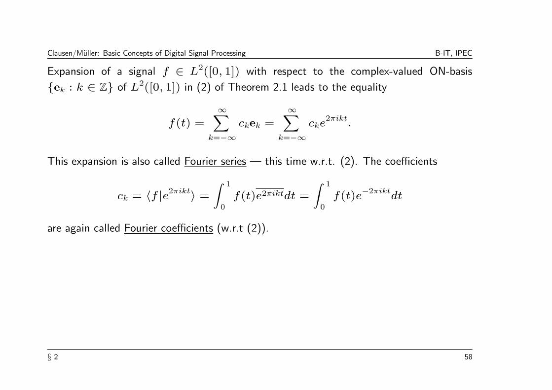
Expansion of a signal f ∈ L2([0, 1]) with respect to the complex-valued ON-basis
ek : k ∈ Z of L2([0, 1]) in (2) of Theorem 2.1 leads to the equality
f(t) =
∞∑
k=−∞ckek =
∞∑
k=−∞cke
2πikt.
This expansion is also called Fourier series — this time w.r.t. (2). The coefficients
ck = 〈f |e2πikt〉 =
∫ 1
0
f(t)e2πiktdt =
∫ 1
0
f(t)e−2πikt
dt
are again called Fourier coefficients (w.r.t (2)).
§ 2 58

Clausen/Muller: Basic Concepts of Digital Signal Processing B-IT, IPEC
The real and complex Fourier transform are closely related. Recall that e2πikt =
cos(2πkt) + i sin(2πkt). Then it is easy to see that
c0 = a0
ck =1√2ak − i
1√2bk, k > 0,
ck =1√2a−k + i
1√2b−k, k < 0,
Similarly ak and bk can be recovered from the ck. For notational reasons, the Fourier
series w.r.t (2) is much easier to deal with. Therefore, we consider in the following only
the Fourier series w.r.t. (2).
§ 2 59
Clausen/Muller: Basic Concepts of Digital Signal Processing B-IT, IPEC
Note 2.2. The equality in the Fourier expansion is just an equality in the L2-sense, i.e.,
equality up to a null set. Under additional conditions on f one also has pointwise equality.
For example, in case f is continuously differentiable the Fourier series converges uniformly
on [0, 1] to f .
§ 2 60

Clausen/Muller: Basic Concepts of Digital Signal Processing B-IT, IPEC
The following theorem says that L2([0, 1]) can be identified with `2(Z) via the Fourier
coefficients. This is a special case of the general theory of Hilbert spaces and ON-systems
(Parseval identity)
Theorem 2.3. The function
f 7→ f := (〈f |ek〉)k∈Z,
which assign to each signal f ∈ L2([0, 1]) the sequence of Fourier coefficients, is a
Hilbert space isomorphism:
L2([0, 1])
'−→ `2(Z).
In particular, for f, g ∈ L2([0, 1]) holds
〈f |g〉L2([0,1]) = 〈f |g〉l2(Z).
§ 2 61

Clausen/Muller: Basic Concepts of Digital Signal Processing B-IT, IPEC
The general case L2([a, b]) for a, b ∈ R, a < b, consisting of λ-periodic functions with
λ = b− a can be easily reduced to the above case a = 0 and b = 1. For example, the
Fourier series transfers to the general case as follows.
Lemma 2.4. Let f ∈ L2([a, b]). Then one obtains the following representation as
Fourier series of f :
f(t) =
∞∑
k=−∞cke
2πiktb−a .
with coefficients
ck =1
b− a
∫ b
a
f(t)e−2πiktb−a dt.
§ 2 62

Clausen/Muller: Basic Concepts of Digital Signal Processing B-IT, IPEC
2.2 Fourier Integral for non-periodic CT-Signals
For non-periodic continuous-time signals one can generalize the idea of the Fourier series.
However, in this case the frequencies of integer values k ∈ Z do, in general, not suffice
to “describe” a signal completely. Considering all frequencies ω ∈ R and replacing
summation by integration one gets the following “continuous” analog to the Fourier series:
Theorem 2.5. For each signal f ∈ L1(R) ∩ L2(R) holds the equality
f(t) =
∫ ∞
−∞cωe
2πiωtdω (1)
where cω is defined by
cω =
∫ ∞
−∞f(t)e
−2πiωtdt. (2)
§ 2 63

Clausen/Muller: Basic Concepts of Digital Signal Processing B-IT, IPEC
Note 2.6. In the following let eω: R → C denote the continuous exponential or frequency
functions t 7→ e2πiωt of frequency ω ∈ R.
(i) The assumption f ∈ L1(R) ∩ L2(R) is a technical condition such that all integrals
involved exist (i.e., are finite). Actually, there are even weaker conditions on f such
that the integrals stills exist.
(ii) The equality (1) shows that any signal f (which satisfies a certain integrability
condition) can be written as a (continuous) superposition of the frequency functions
eω.
(iii) The number cω expresses the “intensity” with which the frequency function eω is
“contained” in the signal f . Hence the numbers cω now play the role of the Fourier
coefficients ck in the Fourier series.
(iv) Note that the frequency functions eω are 1ω-periodic and are not contained in Lp(R)
for 1 ≤ p < ∞.
§ 2 64

Clausen/Muller: Basic Concepts of Digital Signal Processing B-IT, IPEC
Definition 2.7. Let f ∈ L1(R) then the function f : R → C defined by
f(ω) := cω =
∫ ∞
−∞f(t)e
−2πiωtdt, ω ∈ R,
is called Fourier integral or Fourier transform of f . Sometimes f is also denoted by F (f).
It can be shown, that the definition of a Fourier transform of functions f ∈ L1(R)∩L2(R)
can be extended to all signals f ∈ L2(R). (This is a non-trivial mathematical construction
using the so-called Hahn-Banach Theorem.) The next theorem says that the Fourier
transform is invariant under the inner product and hence preserves energy.
Theorem 2.8. (Plancherel) The Fourier transform f 7→ f defines a unitary
transformation on L2(R). Hence, for f ∈ L2(R) holds f ∈ L2(R) and ||f || = ||f ||.Furthermore, one has 〈f |g〉 = 〈f |g〉 for any two functions f, g ∈ L2(R).
§ 2 65

Clausen/Muller: Basic Concepts of Digital Signal Processing B-IT, IPEC
Theorem 2.9. Let f ∈ L1(R) ∩ L2(R) (or more general f ∈ L2(R). Then the Fourier
transform has the following properties:
(1) For t0 ∈ R, the translation of f by t0 is defined by
ft0(t) := f(t− t0).
Then
ft0(ω) = e−2πiωt0f(ω).
(2) For ω0 ∈ R, the modulation of f by ω0 is defined by
fω0(t) := e
−2πiω0tf(t).
Then
fω0(ω) = f(ω + ω0).
(3) Let f be differentiable with f ′ ∈ L2(R). Then
f ′(ω) = 2πiωf(ω).
§ 2 66

Clausen/Muller: Basic Concepts of Digital Signal Processing B-IT, IPEC
(4) Let f be differentiable. Then
f′(ω) = −2πi (t 7→ tf(t))(ω).
(5) For s ∈ R \ 0 the scaled function t 7→ f(t/s) by s is also in L2(R) and
f( ·s)(ω) = sf(ωs).
Proof: The proof, which amounts to a straightforward computation, is left as an exercise.
§ 2 67

Clausen/Muller: Basic Concepts of Digital Signal Processing B-IT, IPEC
Definition 2.10. Let g ∈ L2(R) ∩L1(R). The inverse Fourier transform of g is denoted
by g and defined by the integral
g(t) :=
∫ ∞
−∞g(ω)e
2πitωdω.
It is easy to see that one has g(t) = g(−t). It is more difficult to show the next theorem
whose proof can be found in [Folland].
Theorem 2.11. Let g = f be the Fourier transform of some signal f ∈ L2(R). Then
g ∈ L2(R) and g = f. In other words, one has the identities
(f)∨
= f = (f)∧.
§ 2 68

Clausen/Muller: Basic Concepts of Digital Signal Processing B-IT, IPEC
Example 2.12. In this example, the CT-function f is a superposition of two sines of
frequency 1 Hz and 5 Hz on the interval [0, 10] and zero outside this interval. The
ripples in the spectrum come from the discontinuity of the signal at the boundaries
; “destructive interference”.
0 1 2 3 4 5 6 7 8 9 10−2
−1
0
1
2
Time t
f(t)=sin(2*π*t)+sin(10*π*t)
0 1 2 3 4 5 6 70
5
10
15
20
25
30
Frequency ω
Spectral energy density |F(f)|2
§ 2 69

Clausen/Muller: Basic Concepts of Digital Signal Processing B-IT, IPEC
Example 2.13. For the chirp signal f defined by f(t) = sin(50 · πt2), the frequency ω0
at time t = t0 is roughly given by derivative of the phase divided by 2π, i.e., ω0 = 50 · t0.Note that in the figure below, f is only defined on [0 : 2] and zero outside this interval
; frequency band [−100 : 100] and ripples.
0 0.2 0.4 0.6 0.8 1 1.2 1.4 1.6 1.8 2−1.5
−1
−0.5
0
0.5
1
1.5
Time t
Chirp signal f(t)=sin(50*pi*t2) on the interval [0:2]
−150 −100 −50 0 50 100 1500
1
2
3
4
5
6
7x 10⁻³
Frequency ω
Spectral energy density |F(f)|2
§ 2 70
Clausen/Muller: Basic Concepts of Digital Signal Processing B-IT, IPEC
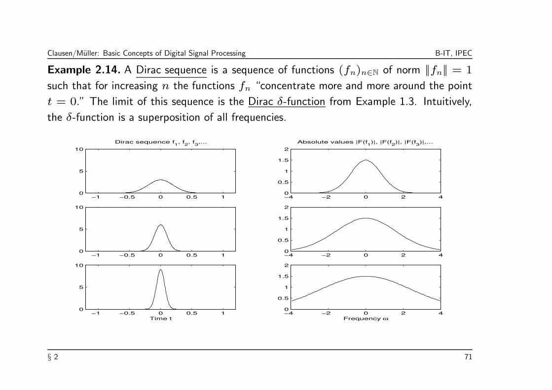
Example 2.14. A Dirac sequence is a sequence of functions (fn)n∈N of norm ||fn|| = 1
such that for increasing n the functions fn “concentrate more and more around the point
t = 0.” The limit of this sequence is the Dirac δ-function from Example 1.3. Intuitively,
the δ-function is a superposition of all frequencies.
−1 −0.5 0 0.5 10
5
10
Dirac sequence f1, f
2, f
3,...
−4 −2 0 2 40
0.5
1
1.5
2
Absolute values |F(f1)|, |F(f
2)|, |F(f
3)|,...
−1 −0.5 0 0.5 10
5
10
−4 −2 0 2 40
0.5
1
1.5
2
−1 −0.5 0 0.5 10
5
10
Time t−4 −2 0 2 40
0.5
1
1.5
2
Frequency ω
§ 2 71

Clausen/Muller: Basic Concepts of Digital Signal Processing B-IT, IPEC
Example 2.15. The Gaussian function defined by the formula
f(t) = (2π)−1
2π−1
4e−πt2
has the remarkable property that it coincides with its Fourier transform. It has the minimal
uncertainty in the sense of Heisenberg’s uncertainty principle (see Chapter 6) and has
good localizing properties in time as well as in frequency.
−2 −1 0 1 20
0.05
0.1
0.15
0.2
0.25
0.3
0.35Gaussian function f
−2 −1 0 1 20
0.05
0.1
0.15
0.2
0.25
0.3
0.35Absolute value |F(f)|
−2 −1 0 1 20
0.05
0.1
0.15
0.2
0.25
0.3
0.35Real part re(F(f))
−2 −1 0 1 2−1
−0.5
0
0.5
1Imaginary part im(F(f))
§ 2 72

Clausen/Muller: Basic Concepts of Digital Signal Processing B-IT, IPEC
Example 2.16. The box function f = b1/2 = χ[−1/2,1/2] of length 1 centered at 0 (see
Example 1.2) is given by
f(t) :=
1 if −1/2 ≤ t ≤ 1/2,
0 elsewhere.
We compute the Fourier transform of f considering first the case for ω 6= 0:
f(ω) =
∫ ∞
−∞f(t)e
−2πiωtdt =
∫ 1/2
−1/2
e−2πiωt
dt
=
[1
−2πiωe−2πiωt
]1/2
−1/2
=1
−2πiω
(e−πiω − e
πiω)
=sin(πω)
πω.
For ω = 0 we get
f(0) =
∫ ∞
−∞f(t)dt = 1.
§ 2 73

Clausen/Muller: Basic Concepts of Digital Signal Processing B-IT, IPEC
In other words, the Fourier transform of the box function is the sinc function from Example
1.4. The Fourier transform is in this case a real-valued function, i.e., the imaginary part of
f is zero as is shown in the following figure.
−1 −0.5 0 0.5 10
0.2
0.4
0.6
0.8
1
Box function f
−4 −2 0 2 40
0.2
0.4
0.6
0.8
1
Absoulte value |F(f)|
−4 −2 0 2 4−1
−0.5
0
0.5
1
re(F(f)) (sinc function)
−4 −2 0 2 4−1
−0.5
0
0.5
1
im(F(f))
§ 2 74

Clausen/Muller: Basic Concepts of Digital Signal Processing B-IT, IPEC
A translation of the signal in the time domain leads to a modulation in the Fourier domain.
This is expressed in formula (1) of Theorem 2.9 and illustrated for the box function in the
next two figures.
Translation of the box function by 1.
0 0.5 1 1.5 20
0.2
0.4
0.6
0.8
1
Box function f
−4 −2 0 2 40
0.2
0.4
0.6
0.8
1
Absolute value |F(f)|
−4 −2 0 2 4−1
−0.5
0
0.5
1
re(F(f))
−4 −2 0 2 4−1
−0.5
0
0.5
1
im(F(f))
§ 2 75

Clausen/Muller: Basic Concepts of Digital Signal Processing B-IT, IPEC
Translation of the box function by 11.
10 10.5 11 11.5 120
0.2
0.4
0.6
0.8
1
Box function f
−4 −2 0 2 40
0.2
0.4
0.6
0.8
1
Absolute value |F(f)|
−4 −2 0 2 4−1
−0.5
0
0.5
1
re(F(f))
−4 −2 0 2 4−1
−0.5
0
0.5
1
im(F(f))
§ 2 76

Clausen/Muller: Basic Concepts of Digital Signal Processing B-IT, IPEC
2.3 Fourier Transform for DT-Signals
In this section, we want to transfer the concept of a Fourier transform to the time-discrete
case. The following definition is a kind of dual concept to the Fourier series:
Definition 2.17. The discrete-time (DT) Fourier transform x of a DT-signal x ∈ `2(Z)
is defined by
x(ω) :=∞∑
k=−∞x(k)e
−2πikω, for ω ∈ [0, 1].
Note 2.18. In Section 1 we have seen that for a periodic function f ∈ L2([0, 1]) the
Fourier transform f := (〈f |e2πikt〉)k∈Z is a DT-signal f ∈ `2(Z) consisting of the
Fourier coefficients. Now, for a DT-signal x ∈ `2(Z), the Fourier transform is a periodic
function x ∈ L2([0, 1]).
§ 2 77
Clausen/Muller: Basic Concepts of Digital Signal Processing B-IT, IPEC
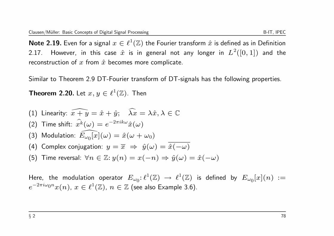
Note 2.19. Even for a signal x ∈ `1(Z) the Fourier transform x is defined as in Definition
2.17. However, in this case x is in general not any longer in L2([0, 1]) and the
reconstruction of x from x becomes more complicate.
Similar to Theorem 2.9 DT-Fourier transform of DT-signals has the following properties.
Theorem 2.20. Let x, y ∈ `1(Z). Then
(1) Linearity: x+ y = x+ y; λx = λx, λ ∈ C
(2) Time shift: xk(ω) = e−2πikωx(ω)
(3) Modulation: Eω0[x](ω) = x(ω + ω0)
(4) Complex conjugation: y = x ⇒ y(ω) = x(−ω)
(5) Time reversal: ∀n ∈ Z: y(n) = x(−n) ⇒ y(ω) = x(−ω)
Here, the modulation operator Eω0: `1(Z) → `1(Z) is defined by Eω0
[x](n) :=
e−2πiω0nx(n), x ∈ `1(Z), n ∈ Z (see also Example 3.6).
§ 2 78

Clausen/Muller: Basic Concepts of Digital Signal Processing B-IT, IPEC
We compare the CT-Fourier transform and the DT-Fourier transform. Let f ∈ L2(R) be
a continuous CT-signal and x ∈ `2(Z) the DT-signal defined by x(k) := f(k), k ∈ Z.
In other words, x is a sampled version of f . By definition we have
f(ω) :=
∫ ∞
−∞f(t)e
−2πiωtdt
and
x(ω) :=∞∑
k=−∞f(k)e
−2πiωk.
Hence, x(ω) is a Riemann sum for f(ω) for each ω ∈ R.
However, note that for increasing |ω| the functions t 7→ f(t)e−2πiωt, t ∈ R are
increasingly oscillating. However, the sampled versions k 7→ f(k)e−2πiωk, k ∈ Z, are
not able to recognize oscillations of frequency greater one since such oscillations take
place between two neighboring time points. This effect is known as aliasing and will be
discussed in Chapter 4 in detail.
§ 2 79

Clausen/Muller: Basic Concepts of Digital Signal Processing B-IT, IPEC
Note 2.21. Fourier series are ideal for analyzing periodic signals, since the harmonic
modes ek, k ∈ Z, unsed in the expansion are themselves periodic. By contrast, the
Fourier intergral transform is a far less natural tool because it uses periodic functions to
expand nonperiodic signals.
§ 2 80

Clausen/Muller: Basic Concepts of Digital Signal Processing B-IT, IPEC
2.4 Discrete Fourier Transform
Computing the Fourier transform of a CT-signal or Fourier coefficients of a periodic
CT-signal involves the evaluation of integrals which is computational infeasible. Also
computing approximation of such integrals via Riemann sums can be very expensive.
Therefore one has to find fast algorithms for computing suitable approximations of Fourier
coefficients for suitable frequencies — possibly at the expense of precision. In real
world applications one usually has to deal with finite DT-signals. Let N ∈ N and
ΩN := e−2πi/N . (ΩN is a so-called Nth primitive root of unity.) The next figure
illustrates the case for N = 8:
8
§ 2 81

Clausen/Muller: Basic Concepts of Digital Signal Processing B-IT, IPEC
Definition 2.22. The discrete Fourier transform (DFT) of size N is a linear map
CN → C
N given by the N ×N -matrix
DFTN :=1√N
(ΩkjN
)0≤k,j<N
=1√N
1 1 · · · 1 1
1 ΩN · · · Ω(N−2)N Ω
(N−1)N
... ... . . . . . . ...
1 Ω(N−2)N
. . . Ω(N−2)(N−2)N Ω
(N−2)(N−1)N
1 Ω(N−1)N · · · Ω
(N−1)(N−2)N Ω
(N−1)(N−1)N
§ 2 82

Clausen/Muller: Basic Concepts of Digital Signal Processing B-IT, IPEC
Hence, for a vector (finite DT-signal) v := (v0, v1, . . . , vN−1)T ∈ C
N the DFT of v is
again a vector v = DFTN(v) ∈ CN given by
vk :=1√N
N−1∑
j=0
vje−2πijk/N
, k = 0, 1, . . . , N − 1.
Note 2.23. The rows of the DFTN -matrix given by
fk =1√N
(1, (ΩN)k, . . . , (ΩN)
k(N−1))T ∈ C
N, k = 0, 1, . . . N − 1,
are truncated versions of the discrete frequency signals from Example 1.9 and form an
orthonormal basis of CN . Hence for the component vk holds
vk = 〈v|fk〉.
§ 2 83

Clausen/Muller: Basic Concepts of Digital Signal Processing B-IT, IPEC
Note that the straightforward computation of the matrix-vector product DFTN(v)
requires O(N2) multiplications and additions. This is for most applications to slow — in
many cases one has to deal with large N >> 105.
The important point is that there is an efficient algorithm, the so-called
fast Fourier transform (FFT), to compute the DFT of an vector of length N in
O(N logN). We refer for a detailed description of this algorithm to [Clausen/Baum].
The main idea of the FFT-algorithm — originally found by Gauss and rediscovered by
Cooley and Tukey in 1965 — is based on a clever matrix factorization.
§ 2 84

Clausen/Muller: Basic Concepts of Digital Signal Processing B-IT, IPEC
For N = 2M holds:
DFTN ·
v0
v1...
vN−1
=
1√2
(idM ∆M
idM −∆M
)(DFTM 0
0 DFTM
)
v0
v2...
vN−2
v1
v3...
vN−1
Here
idM = diag (1, 1, . . . , 1) and ∆M = diag (1,ΩN , . . . ,ΩM−1N )
denote the M × M -identity matrix and an M × M -diagonal matrix, respectively.
Furthermore, DFTM corresponds to the DFT-matrix for ΩM = Ω2N . If N is a power of
two, this procedure can be performed recursively leading to an upper bound of 32N logN
additions and multiplications.
§ 2 85
Clausen/Muller: Basic Concepts of Digital Signal Processing B-IT, IPEC
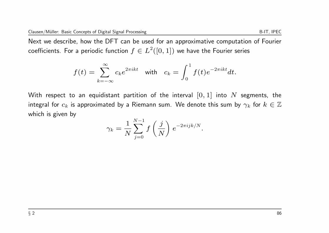
Next we describe, how the DFT can be used for an approximative computation of Fourier
coefficients. For a periodic function f ∈ L2([0, 1]) we have the Fourier series
f(t) =∞∑
k=−∞cke
2πiktwith ck =
∫ 1
0
f(t)e−2πikt
dt.
With respect to an equidistant partition of the interval [0, 1] into N segments, the
integral for ck is approximated by a Riemann sum. We denote this sum by γk for k ∈ Z
which is given by
γk =1
N
N−1∑
j=0
f
(j
N
)e−2πijk/N
.
§ 2 86

Clausen/Muller: Basic Concepts of Digital Signal Processing B-IT, IPEC
By the identity e−2πijk/N = e−2πij(k+N)/N the map
Z → C, k 7→ γk
is N -periodic (this again is the so-called aliasing effect). Hence, the entire information of
the sequence (γk)k∈Z is contained in the vector
Γ := (γ0, γ1, . . . , γN−1)T.
Note that Γ can be computed via the DFT of the vector v := (v0, v1, . . . , vN−1)T ∈ C
N
were vj := 1√Nf( jN ).
Note 2.24. The DFT computes Riemann approximations of N Fourier coefficients
synchronously.
Note 2.25. In general, the quality of the approximation of ck via γk decreases for
increasing k. (Consider the number of oscillations of the function to be integrated!) In
many cases, only half of the numbers γk for 0 ≤ k < N2 give acceptable approximations
for ck.
§ 2 87

Clausen/Muller: Basic Concepts of Digital Signal Processing B-IT, IPEC
Example 2.26. In this example we need the Hanning-window g — a so-called
window function — which is depicted below and defined by
g(u) :=
1 + cos(πu) for −0.5 ≤ u ≤ 0.5
0 otherwise
−0.4 −0.2 0 0.2 0.4 0.60
0.2
0.4
0.6
0.8
1
Time t
Hanning window g
−2 −1 0 1 20
0.05
0.1
0.15
0.2
0.25
Frequency ω
Spectral energy density |F(g)|2
§ 2 88
Clausen/Muller: Basic Concepts of Digital Signal Processing B-IT, IPEC
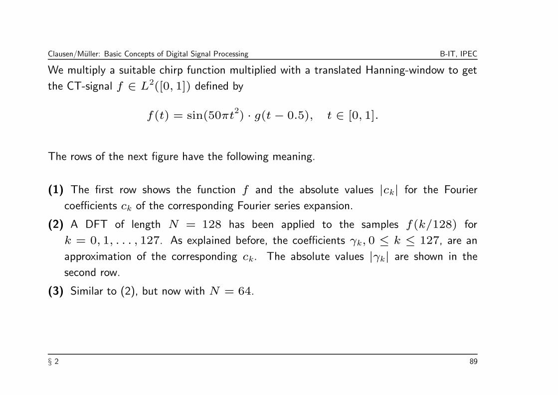
We multiply a suitable chirp function multiplied with a translated Hanning-window to get
the CT-signal f ∈ L2([0, 1]) defined by
f(t) = sin(50πt2) · g(t− 0.5), t ∈ [0, 1].
The rows of the next figure have the following meaning.
(1) The first row shows the function f and the absolute values |ck| for the Fourier
coefficients ck of the corresponding Fourier series expansion.
(2) A DFT of length N = 128 has been applied to the samples f(k/128) for
k = 0, 1, . . . , 127. As explained before, the coefficients γk, 0 ≤ k ≤ 127, are an
approximation of the corresponding ck. The absolute values |γk| are shown in the
second row.
(3) Similar to (2), but now with N = 64.
§ 2 89

Clausen/Muller: Basic Concepts of Digital Signal Processing B-IT, IPEC
0 0.2 0.4 0.6 0.8 1
−1
0
1
f(t)=sin(50⋅ pi⋅ t2)⋅(Hanning window)
0 50 1000
0.05
0.1
Fourier coefficients ck
0 0.2 0.4 0.6 0.8 1
−1
0
1
Sampling rate 1/N, N=128
0 50 1000
0.05
0.1
Approximation γk of c
k, k=0,…,127
0 0.2 0.4 0.6 0.8 1
−1
0
1
Sampling rate 1/N, N=64
0 50 1000
0.05
0.1
Approximation γk of c
k, k=0,…,63
§ 2 90

Clausen/Muller: Basic Concepts of Digital Signal Processing B-IT, IPEC
Example 2.27. The same as in Example 2.26 with f being a box function.
0 0.2 0.4 0.6 0.8 1
−1
0
1
f = box function
0 20 40 60 80 1000
0.05
0.1
Fourier coefficients ck
0 0.2 0.4 0.6 0.8 1
−1
0
1
Sampling rate 1/N, N=88
0 20 40 60 80 1000
0.05
0.1
Approximation γk of c
k, k=0,…,87
0 0.2 0.4 0.6 0.8 1
−1
0
1
Sampling rate 1/N, N=40
0 20 40 60 80 1000
0.05
0.1
Approximation γk of c
k, k=0,…,39
§ 2 91

Clausen/Muller: Basic Concepts of Digital Signal Processing B-IT, IPEC
Chapter 3: Systems and Filters
Andrew S. Glassner writes in his book “Principles of Digital Image Synthesis.” [Glassner]:
Anything that alters a signal my be considered a system. For example, a concert hall
may be considered a system. In this case, think of the sound of a violin as a signal
represented by the amplitude of sound with respect to time. So a concert hall changes
an input signal (a violin played on stage) to an output signal (the particular sound you
hear at some particular seat).
Mathematically, a system T : I → O transforms an input signal x ∈ I into an output
signal y ∈ O. Here I and O denote suitable signal spaces.
x −→ system T −→ y.
§ 3 92

Clausen/Muller: Basic Concepts of Digital Signal Processing B-IT, IPEC
3.1 Linear Filter and LTI-Systems
We just consider the discrete-time case in detail and refer for a summary of the CT-case
to Section 3.5. Mainly we are interested in the case I = `p(Z) = O, 1 ≤ p ≤ ∞. The
easiest class of systems between such spaces are linear systems.
Definition 3.1. Let I and O linear signal spaces. A linear map T : I → O is called a
linear system. One has
T [x+ y] = T [x] + T [y] and T [λx] = λT [x],
for all x, y ∈ I and all λ ∈ C.
Note 3.2. Note that T maps a signal to another signal, whereas a signal itself maps an
element (the time point) into another element (the value of amplitude). In other words,
T is a function between function spaces and is often referred to as an operator. This
is also expressed in using different parenthesis: one often writes T [x] instead of T (x).
Then T [x](n) denotes the value of the output signal T [x] at time n.
§ 3 93

Clausen/Muller: Basic Concepts of Digital Signal Processing B-IT, IPEC
Example 3.3. The time shift by k ∈ Z is defined by
τk[x](n) := x(n− k).
It is easy to see that τk is a linear operator from `p(Z) to `p(Z). Sometimes we also
write write xk for τk[x]. In particular, x0 = x and δk is the indicator function for k ∈ Z,
i.e., δk(j) = δkj for j ∈ Z.
x x2
§ 3 94

Clausen/Muller: Basic Concepts of Digital Signal Processing B-IT, IPEC
Example 3.4. The M -downsampler for some M ∈ N is defined by
(↓M)[x](n) := x(M · n).
This linear operator from `p(Z) to `p(Z) takes only every Mth value of the signal x.
x( 2)[ ]x
k k
§ 3 95

Clausen/Muller: Basic Concepts of Digital Signal Processing B-IT, IPEC
Example 3.5. Der M -upsampler for some M ∈ N is defined by
(↑M)[x](n) =
x(n/M), if M |n,
0, otherwise.
This linear operator from `p(Z) to `p(Z) widens the signal x and inserts M−1 additional
time points with value 0 between any two neighboring time points of x.
x( 2)[ ]x
k k
§ 3 96

Clausen/Muller: Basic Concepts of Digital Signal Processing B-IT, IPEC
Example 3.6. The amplitude modulation with a support signal c ∈ `∞(Z) is defined by
mc[x](n) := c(n) · x(n).
An important special case is the frequency shift operator with respect to some ω ∈ (0, 1)
defined by
Eω[x](n) := e−2πiωn
x(n).
In case of the signal x = fω0=(e2πiω0n
)n∈Z
∈ `∞(Z) we get
Eω[fω0] = fω0−ω.
With respect to composition the operators Eω und E−ω are inverse to each other:
(E−ω) Eω[x] = x.
The operator E−ω is then called demodulation. By using modulation and subsequent
demodulation, signals can be transmitted using high-frequency support signals.
§ 3 97
Clausen/Muller: Basic Concepts of Digital Signal Processing B-IT, IPEC
We finally give two examples of systems which are not linear.
Example 3.7. The quantization operators given by
rounding up: dxe(n) := dx(n)e, for x: Z → R
rounding down: bxc(n) := bx(n)c, for x: Z → R
are not linear. However these operators are time invariant:
dxke = dxek , bxkc = bxck
§ 3 98
Clausen/Muller: Basic Concepts of Digital Signal Processing B-IT, IPEC
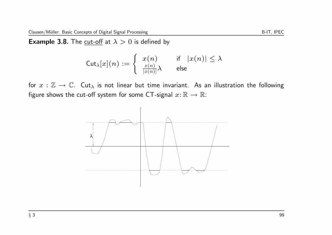
Example 3.8. The cut-off at λ > 0 is defined by
Cutλ[x](n) :=
x(n) if |x(n)| ≤ λx(n)|x(n)|λ else
for x : Z → C. Cutλ is not linear but time invariant. As an illustration the following
figure shows the cut-off system for some CT-signal x: R → R:
λ
§ 3 99

Clausen/Muller: Basic Concepts of Digital Signal Processing B-IT, IPEC
We are interested in linear systems, which do not behave in a pathological way. One such
important property is continuity.
Definition 3.9. A linear system T : `p(Z) → `r(Z) is called continuous, if it maps all
convergent sequences of input signals in `p(Z) to convergent sequences of output signals
in `r(Z).
The following theorem describes a property of continuous operators which is often taken
for granted:
Theorem 3.10. A continuous linear system T : `p(Z) → `r(Z) commutes with infinite
sums. In particular, for x ∈ `p(Z) holds
T [∑
k∈Z
x(k)δk] =
∑
k∈Z
x(k)T [δk].
Note that the opposite statement also holds under certain additional conditions.
§ 3 100
Clausen/Muller: Basic Concepts of Digital Signal Processing B-IT, IPEC
Proof: For n ∈ N let σn :=∑
|k|≤n x(k)δk. Then σn converges to x in the
`p(Z)-norm. Since T is continuous, T [σn] converges to T [x] in the `r(Z)-norm, i.e.,
∥∥∥∥∥∥T [x] −
∑
|k|≤nx(k)T [δ
k]
∥∥∥∥∥∥r
→ 0
for n → ∞. Hence
T [x] = limn→∞
∑
|k|≤nx(k)T [δ
k] =
∑
k∈Z
x(k)T [δk].
§ 3 101
Clausen/Muller: Basic Concepts of Digital Signal Processing B-IT, IPEC
Very important are systems which commute with time shifts.
Definition 3.11. A linear system T : `p(Z) → `r(Z) is called a time invariant if
T τk = τk T for k ∈ Z. In other words, for all k ∈ Z and all x ∈ `p(Z) holds
T [xk] = T [x]
k.
A linear time invariant system is called linear time invariant (LTI) system.
LTI systems can be easily described and characterized by the so-called convolution operator.
This will be the content of the next section.
§ 3 102

Clausen/Muller: Basic Concepts of Digital Signal Processing B-IT, IPEC
3.2 Convolution Filter
The convolution of two signals is a kind of multiplication leading again to a signal.
Convolution plays a crucial role in describing filters and hence is an indispensable
mathematical tool in digital signal processing.
Definition 3.12. Let x, y: Z → C be signals, then the convolution of x and y at position
n ∈ Z is defined to be
(x ∗ y)(n) :=∑
k∈Z
x(k)y(n− k).
Attention: x ∗ y exists only under suitable conditions on x and y, e.g., x ∈ `1(Z), y ∈`∞(Z) or x, y ∈ `2(Z). Further conditions will be summarized in Theorem 3.13.
§ 3 103

Clausen/Muller: Basic Concepts of Digital Signal Processing B-IT, IPEC
Intuitively, if y: Z → C is a signal and x a probability distribution on Z, i.e., x: Z → [0, 1]
with∑
n∈Zx(n) = 1, then (x ∗ y)(n) =
∑k∈Z
x(k)y(n − k) can be thought of as
weighted average of y around the neighborhood of n.
The following figure illustrates this for the position n = 4.
1 2 3 4-1-3-4 -20
0
y
x
§ 3 104

Clausen/Muller: Basic Concepts of Digital Signal Processing B-IT, IPEC
In the following theorem we summarize some important properties of the convolution and
mulitplication operator. For a proof we refer to [Folland].
Theorem 3.13. Let 1 ≤ p, q, r ≤ ∞. Then the following holds.
(1) (Young Inequality) `1 ∗ `p ⊆ `p, i.e., for all x ∈ `1(Z) and y ∈ `p(Z) holds
x ∗ y ∈ `p(Z) and
||x ∗ y||p ≤ ||x||1 · ||y||p.(2) Let p and q be conjugate exponents (i.e., 1
p + 1q = 1 where one sets 1
∞ := 0)).
Then for all x ∈ `p and y ∈ `q holds
x · y ∈ `1
and ||x · y||1 ≤ ||x||p · ||y||qx ∗ y ∈ `
∞and ||x ∗ y||∞ ≤ ||x||p · ||y||q.
(3) For all x ∈ `p(Z) and y ∈ `∞(Z) one has x · y in `p(Z) and
||x · y||p ≤ ||x||p · ||y||∞
§ 3 105

Clausen/Muller: Basic Concepts of Digital Signal Processing B-IT, IPEC
Theorem 3.14. Let x, y, z ∈ CZ and suppose all of the following convolutions and
products in question exist. The pointwise multiplication and convolution of signals are
commutative and associative, i.e.,
x · y = y · x, x ∗ y = y ∗ x,
and
(x · y) · z = x · (y · z), (x ∗ y) ∗ z = x ∗ (y ∗ z).Furthermore, in combination with addition the respective laws of distributivity hold:
(x+ y) · z = x · z + y · z, (x+ y) ∗ z = x ∗ z + y ∗ z.
From this theorem follows that for fixed y ∈ `q(Z) the convolution operator Cy defined
by Cy(x) := x ∗ y is linear. From Theorem 3.13 follows that Cy: `p(Z) → `∞(Z) is
continuous.
§ 3 106
Clausen/Muller: Basic Concepts of Digital Signal Processing B-IT, IPEC
The convolution operator has a the following remarkable behaviour under Fourier transform.
Theorem 3.15. Let x, y ∈ `2(Z) with x ∗ y ∈ `2(Z). Then
x ∗ y = x · y.
In other words, the Fourier transform of the convolution of two signals equals the pointwise
multiplication of the Fourier transforms of the signals.
Note 3.16. The equaltiy in 3.15 holds only in the L2([0, 1])-sense. This implies that
x ∗ y(ω) = x(ω)y(ω) for almost all ω ∈ [0, 1].
§ 3 107

Clausen/Muller: Basic Concepts of Digital Signal Processing B-IT, IPEC
Example 3.17. For x ∈ `∞(Z) holds
τk[x] = xk
= x ∗ δk.
To show this, we first look at the left hand side of the equality:
τk[x](n) = x(n− k).
For the right hand side one has
(x ∗ δk)(n) =∑
`∈Z
x(`)δk(n− `)
=∑
`∈Z
x(`)δ`=n−k
= x(n− k)
In other words, the time shift operator τk coincides with the convolution operator Cδk on
`∞(Z).
§ 3 108

Clausen/Muller: Basic Concepts of Digital Signal Processing B-IT, IPEC
Generalizing the previous example one gets the following theorem:
Theorem 3.18. Let 1 ≤ p, q ≤ ∞ and T : `p(Z) → `q(Z) a continuous LTI system.
Define h := T [δ], then T = Ch, i.e., for all x ∈ `p(Z) holds
T [x] = h ∗ x.
Proof: Since δ ∈ `p(Z) the sequence h := T [δ]`q(Z) is well defined. Furthermore, for
all n ∈ Z and x ∈ `p(Z) holds
T [x](n) = T [∑
k
x(k)δk](n)
=∑
k
x(k)T [δk](n) (linearity and continuity of T )
=∑
k
x(k)T [δ]k(n) (time invariance of T )
=∑
k
x(k)h(n− k) = (h ∗ x)(n).
§ 3 109

Clausen/Muller: Basic Concepts of Digital Signal Processing B-IT, IPEC
The previous theorem showed that continuous LTI systems can be expressed by a
convolution operator. If we impose further conditions on the LTI systems they are even
characterized by convolution.
Definition 3.19. A linear system T : `p(Z) → `p(Z) is called stable if
(1) T is continuous and
(2) ∀k ∈ Z:T [δk] ∈ `1(Z)
In the case p = ∞ one also speaks from BIBO-stable (Bounded Input → Bounded
Output) linear systems.
§ 3 110
Clausen/Muller: Basic Concepts of Digital Signal Processing B-IT, IPEC
Theorem 3.20. For a linear system T : `p(Z) → `p(Z) the following is equivalent:
(1) T is a stable LTI system.
(2) There is an h ∈ `1(Z) with T = Ch, i.e., T [x] = h ∗ x, for all x ∈ `p(Z).
Proof: (1) ⇒ (2): See the proof of Theorem 3.18.
(2) ⇒ (1): Linearity is clear. Time invariance follows from the associativity of
convolution:
T [xk] = h ∗ (x
k) = h ∗ (x ∗ δk) = (h ∗ x) ∗ δk = T [x]
k.
Continuity follows from Theorem 3.13 which implies
||h ∗ (x− xm)||p ≤ ||h||1 · ||x− xm||p → 0 for m → ∞
for xm → x in `p(Z).
§ 3 111

Clausen/Muller: Basic Concepts of Digital Signal Processing B-IT, IPEC
Definition 3.21. Let T be a continuous LTI-System and h := T [δ].
(1) The sequence h is called the impulse response of the system and h(n) is called the
nth filter coefficient.
(2) T is called FIR filter or FIR system (Finite Impulse Response) if only a finite number
of filter coefficients are non zero. Otherwise T is called IIR filter or IIR system (Infinite
Impulse Response).
Note 3.22. Very often one identifies the filter T with the impulse response h. Therefore,
one often simply speaks of the filter h meaning the underlying convolution filter Ch.
§ 3 112

Clausen/Muller: Basic Concepts of Digital Signal Processing B-IT, IPEC
Definition 3.23. The length `(x) of non-zero DT-signal x ∈ CZ (i.e., xn = 0 for all
n ∈ Z but a finite number) is defined by
`(x) := 1 + maxn|x(n) 6= 0 − minn|x(n) 6= 0.
In other words, if a ∈ Z is the smallest index with x(a) 6= 0 and b ∈ Z the largest index
with x(b) 6= 0, then `(x) := b− a+ 1.
If h 6= 0 is the impulse response of some FIR filter, then `(h) is also called the length of
the FIR filter.
Lemma 3.24. The length of the convolution of two finite sequences x and y is given by
the formula
`(x ∗ y) = `(x) + `(y) − 1.
Proof: The proof is left as an exercise.
§ 3 113

Clausen/Muller: Basic Concepts of Digital Signal Processing B-IT, IPEC
Figure 6: Example for the impulse response of an FIR filter of length 8
§ 3 114

Clausen/Muller: Basic Concepts of Digital Signal Processing B-IT, IPEC
Definition 3.25. Let T be a continuous LTI-System and h := T [δ]. T is called causal if
h(n) = 0 for n < 0.
In [Proakis/Manolakis, p. 69] the importance of causality is explained as follows:
It is apparent that in real-time signal processing applications we cannot observe the
future values of the signal, an hence a noncausal system is physically unrealizable
(i.e., it cannot be implemented). On the other hand, if the signal is recorded so that
the processing is done off-line (nonreal time), it is possible to implement a noncausal
system, since all values of the signal are available at the time of processing. This is
often the case in the processing of geophysical signals and images.
§ 3 115

Clausen/Muller: Basic Concepts of Digital Signal Processing B-IT, IPEC
Example 3.26. A causal FIR filter T of order N and length N + 1 is of the form
T [x](n) =
N∑
`=0
h(`)x(n− `)
with filter coefficients h(0), . . . , h(N), h(N) 6= 0, and h(0) 6= 0. The output signal
T [x] depends at time point n only on the “past” x(n − 1), . . . , x(n − N) and the
“present” x(n) of the input signal x. (Therefore one speaks of causality.) These values
are weighted with the filter coefficients and added up.
§ 3 116

Clausen/Muller: Basic Concepts of Digital Signal Processing B-IT, IPEC
Example 3.27. The time shifts satisfy τk τ` = τk+` = τ` τk and are therefore time
invariant operators. Since τk[δ] = δk ∈ `1(Z), the time shifts are stable LTI systems and
coincide with the convolution operator: τk = Cδk. In particular, τk is an FIR system and
for k ≥ 0 it is causal.
Example 3.28. The downsampler (↓M) is linear and continuous. Note that (↓M)[δk]
is zero in the case that k is a multiple of M , and otherwise it is δk/M . Hence the
downsampler is a stable system. However, it is not time invariant since
((↓M) τk)[x](n) = x(nM − k) but (τk (↓M))[x](n) = x(n(M − k)).
Similarly, the upsampler (↑M) is also linear, continuous, and stable, but not time
invariant.
§ 3 117

Clausen/Muller: Basic Concepts of Digital Signal Processing B-IT, IPEC
Example 3.29. The frequency shift operator Eω defined by Eω[x](n) := e−2πiωn ·x(n)
is linear and continous. However, in general it is not time invariant. To be more specific,
it holds
(Eω τk)[x](n) = Eω[xk](n) = e
−2πiωnx(n− k)
which is in general not equal to
(τk Eω)[x](n) = Eω[x](n− k) = e−2πiω(n−k)
x(n− k).
Eω commutes with all τk, k ∈ Z, if and only if e2πiωk = 1 for all k ∈ Z. This only
holds for the case ω = 0.
Further examples will be given in Chapter 5.
§ 3 118

Clausen/Muller: Basic Concepts of Digital Signal Processing B-IT, IPEC
3.3 Frequency Response
To characterize certain properties of an LTI system the Fourier transform of the
corresponding impulse response plays — as we will see later — a crucial role.
Definition 3.30. Let T be a BIBO-stable LTI system with impulse response h = T [δ] ∈`1(Z). Then the Fourier transform (see Definition 2.17)
h(ω) :=∞∑
n=−∞h(n)e
−2πinω, ω ∈ [0, 1],
is called frequency response of T .
§ 3 119
Clausen/Muller: Basic Concepts of Digital Signal Processing B-IT, IPEC
Note 3.31. In the literature one can find the following conventions which we will also use
in the rest of this lecture.
(i) Identifying the system T with its impulse response h one often speaks from the
frequence response h of the filter h. One then also writes H instead of h.
(2) More general, one often uses small letters f, g, h, . . . , x, y . . . to denote the discrete
filters and DT-signals. The corresponding Fourier transforms are then denoted by the
corresponding capital letters F,G,H, . . . , X, Y . . ..
§ 3 120

Clausen/Muller: Basic Concepts of Digital Signal Processing B-IT, IPEC
Theorem 3.32. Let T = Ch, i.e., T [x] = h ∗ x, be a BIBO-stable LTI system. Then
the frequency response H(ω) :=∑
k∈Zh(k)e−2πiωk at ω ∈ [0, 1] is an eigenvalue
of T . The frequency sequence fω := (e2πiωn)n∈Z ∈ l∞(Z) of frequency ω is an
eigenvector to this eigenvalue, i.e.,
T [fω] = H(ω)fω.
The proof is left as an exercise which amounts to a straightforward computation. We have
seen that a BIBO-stable LTI system maps a (normalized) frequency series of frequency ω
into the H(ω)-multiple of the same frequency series.
§ 3 121

Clausen/Muller: Basic Concepts of Digital Signal Processing B-IT, IPEC
Definition 3.33. Let h(ω) = H(ω) =∑
n∈Zh(n)e−2πiωn be the frequency response
of some filter h ∈ `(Z). Then the representation of H in polar coordinates is given by
H(ω) = |H(ω)| · e2πiΦh(ω).
The function
ω 7→ |H(ω)|is called the magnitude response of h , whereas the function
ω 7→ Φh(ω)
is called phase response of h. Furthermore, the spectral energy density is defined to be
the function
ω 7→ |H(ω)|2.
§ 3 122

Clausen/Muller: Basic Concepts of Digital Signal Processing B-IT, IPEC
In digital signal processing it is usual to see the magnitude response displayed in decibels
(dB). The decibel function dB: R>0 → R is defined by
dB(r) := 20 log10(r)
for positive real numbers r. Note that dB is monotonously decreasing, dB(1) = 0 and
limr→0
dB(r) = −∞.
Hence the decibel function is suitable to study the behavior of positive functions close to
0. To get a feeling for decibels, observe that
dB(2r) ≈ 6 + dB(r),
i.e., doubling of the input corresponds to an increase of about 6 decibels.
The magnitude response measured in dB is given by
ω 7→ 20 log10 |H(eiω
)|.
§ 3 123

Clausen/Muller: Basic Concepts of Digital Signal Processing B-IT, IPEC
Example 3.34. The following figure shows the magnitude response |H| and the phase
response Φh of a filter h of length 15. The non-zero filter coefficients of h
are h(−7) = −0.0036 = h(7), h(−5) = 0.0161 = h(5), h(−3) = −0.0682 =
h(3), h(−1) = 0.3038 = h(1), and h(0) = 0.5. The characteristics of |H| can be
better seen in the decibel-scale.
−5 0 5−0.2
0
0.2
0.4
0.6Filter h of length 15
0 0.25 0.5 0.75 10
0.2
0.4
0.6
0.8
1
Magnitude response |H|
0 0.25 0.5 0.75 1−4
−2
0
2
4
Phase response Φh
0 0.25 0.5 0.75 1−80
−60
−40
−20
0
20Magnitude response |H| in dB
§ 3 124

Clausen/Muller: Basic Concepts of Digital Signal Processing B-IT, IPEC
Note 3.35. The frequency response H of a filter h exhibits the so-called
spectral information of h. It has the following properties.
(1) For a real-valued filter h one has H(ω) = H(−ω). Therefore the magnitude
response is an even function, i.e., |H(ω)| = |H(−ω)|, whereas the phase response
is an odd function, i.e., Φh(−ω) = −Φh(ω).
(2) The frequency response is a 1-periodic function. Since for real-valued filters h the
frequency response satisfies H = H, all information of H is already given by the
interval [0, 12].
(3) Spectral information corresponding to low frequencies correspond to ω ∈ [0, 12]
around 0 whereas spectral information corresponding to high frequencies correspond to
ω ∈ [0, 12] around 1
2.
§ 3 125

Clausen/Muller: Basic Concepts of Digital Signal Processing B-IT, IPEC
From Theorem 3.15 follows that convolution of an input signal x with the filter h changes
the frequency content X = x of the signal by pointwise multiplication with the frequency
response H of the filter: depending on the properties of the magnitude response |H| one
distinguishes between lowpass, highpass, and bandpass filter.
Definition 3.36. Let ω0, ω1 ∈ [0, 12], ω1 < ω2 denote a so-called cut-off frequency and
h be a real-valued filter.
(1) h is called lowpass filter, if low frequencies ω with 0 ≤ ω ≤ ω0 are let through
without attenuation whereas high frequencies ω with ω0 ≤ ω ≤ 12 are cut off. In
other words,
|H(ω)| ≈
1 if |ω| ∈ [0, ω0]
0 if |ω| ∈ [ω0,12]
(2) Similarly h is called highpass filter if
|H(ω)| ≈
1 if |ω| ∈ [ω0,12]
0 if |ω| ∈ [0, ω0]
§ 3 126

Clausen/Muller: Basic Concepts of Digital Signal Processing B-IT, IPEC
(3) Similarly h is called bandpass filter if
|H(ω)| ≈
1 if |ω| ∈ [ω0, ω1]
0 if |ω| ∈ [0, ω0] ∪ [ω1,12]
(a)
1/2 1/2
(b)
1/2
(c)
1/4 1/4 1/4
ω ω ω
Figure 7: Magnitude responses of an ideal (a) lowpass, (b) highpass and (c) bandpass
filter.
§ 3 127

Clausen/Muller: Basic Concepts of Digital Signal Processing B-IT, IPEC
3.4 z-Transform and Transfer Function
The z-transform is a generalization of the discrete-time Fourier transform that allows many
signals not having a Fourier transform to be described using related transform techniques.
Definition 3.37. Let x: Z → C be a signal. The z-transform of x, denoted by X, is
defined to be the series
X(z) :=∑
n∈Z
x(n)z−n,
in the complex variable z.
Note 3.38. In complex analysis, series of the form∑
n∈Zx(n)z−n are also called
Laurent series.
Note that when z = e2πiω, the z-transform becomes the discrete-time Fourier transform
X(e2πiω
) =∑
n∈Z
x(n)e−2πinω
.
§ 3 128
Clausen/Muller: Basic Concepts of Digital Signal Processing B-IT, IPEC
As with the DT-Fourier transform, the z-transfrom is only defined when the sum in
Definition 3.37 converges. The sum generally does not converge for all values z ∈ C.
Definition 3.39. Let X be the z-transform of the DT-signal x: Z → C, then the
region of convergence, denoted by Dx, is the largest open subset of C for which elements
z ∈ Dx the infinite series∑
n∈Zx(n)z−n converges.
Note 3.40. The symbol X denotes the z-transform as well as the DT-Fourier transform
(or frequency response) of some DT-signal x. This might be confusing since, for
example, the z-transform X(e2πiω) at z = e2πiω equals the DT-Fourier transfrom
X(ω). However, from the context it should be clear which transform is meant.
§ 3 129

Clausen/Muller: Basic Concepts of Digital Signal Processing B-IT, IPEC
The following theorem shows that the region of convergence Dx is an (possibly empty)
annulus which is also illustrated by the figure below.
Theorem 3.41. Let x: Z → C be a signal. Then the region of convergence Dx is an
open annulus with inner radius Ri(x) and outer radius Ra(x), where
Ri(x) = limn→∞|x(n)|1/n and Ra(x) =1
limn→∞|x(−n)|1/n.
Hence, Dx = z ∈ C | Ri(x) < |z| < Ra(x).
Ri
Dh
aR
§ 3 130

Clausen/Muller: Basic Concepts of Digital Signal Processing B-IT, IPEC
Example 3.42. If x : Z → C is of finite length, i.e., h(n) 6= 0 only for a finite number
of n ∈ Z, then
Ri(h) = 0 and Ra(h) = ∞.
In other words, the region of concergence of the z-transform of a finite signal is C \ 0.
The following theorem shows, that two complex functions which are defined by Laurent
series are equal if and only if all coefficients of the Laurent series coincide.
Theorem 3.43. [Identity theorem for Laurent series.] Let∑
n∈Zxnz
n and∑n∈Z
ynzn be two Laurent series which converge on the circle Sρ of radius ρ > 0
around 0 uniformly to the same limit function f . Then for n ∈ Z holds
xn = yn =1
2πρn
∫ 2π
0
f(ρ · eiϕ)e−inϕdϕ.
The assumption are fulfilled if Sρ ⊂ Dx ∩Dy.
Proof: See [Remmert], p. 284.
§ 3 131

Clausen/Muller: Basic Concepts of Digital Signal Processing B-IT, IPEC
What can be said about the order of magnitude of the signal values x(n) and the region
of convergence? The following theorem gives, in part, an answer.
Theorem 3.44. Let x: Z → R and ρ ∈ R with Ri(x) < ρ < Ra(x). Furthermore,
let µρ := max|z|=ρ |X(z)| denote the maximum of the z-transform X on the circle
of radius ρ. Then the so called Gutzmersch formula holds:
∑
n∈Z
|x(n)|2ρ−2n=
1
2π
∫ 2π
0
|X(ρ · eiϕ)|2dϕ ≤ µ2ρ.
In addition, the Cauchy inequality holds:
|x(n)| ≤ µρ · ρn.
Proof: See [Remmert], p. 285.
By the Gutzmersch formula the sequence (x(n)ρ−n)n∈Z is in `2(Z). In the case
0 < ρ < 1 the sequence x, if it is causal, is absolutely summable.
§ 3 132

Clausen/Muller: Basic Concepts of Digital Signal Processing B-IT, IPEC
The z-transform has many properties generalizing the properties of the DT-Fourier
transform (see Theorem 2.20).
Theorem 3.45. Let x, y and h DT-signals Z → C with z-transforms X,Y and H,
respectively. Then the following holds.
(1) Linearity: Let D be an open subset of C and L(D) be the set all signals x: Z → C
such that D ⊆ Dx. Then the map
L(D) 3 x 7→ X ↓ D
is linear, where X ↓ D denotes the restriction of the z-transform to D.
(2) Time shift: Let y = xk, i.e., y(n) = x(n − k), then Dy = Dx and
Y (z) = z−kX(z).
(3) Modulation: Let a ∈ C \ 0 and y(n) = anx(n), then Dy = |a| · Dx and
Y (z) = X(z/a).
(4) Complex conjugation: If y(n) = x(n) for all n ∈ Z, then Dy = Dx and
Y (z) = X(z).
§ 3 133

Clausen/Muller: Basic Concepts of Digital Signal Processing B-IT, IPEC
(5) Time reversal: If y(n) = x(−n) for all n ∈ Z, then Dy = D−1x and
Y (z) = X(z−1).
(6) Convolution: If y = h ∗ x, then for all z ∈ Dh ∩Dx ⊆ Dy holds
Y (z) = H(z) ·X(z).
Proof: We give the proof for some of the properties and leave the rest as an exercise.
(2) Time shift:
Y (z) =∑
n∈Z
y(n)z−n
=∑
n∈Z
x(n− k)z−n
=∑
n∈Z
x(n− k)z−(n−k)
z−k
= z−k∑
n∈Z
x(n− k)z−(n−k)
= z−k∑
n∈Z
x(n)z−n
= z−kX(z)
§ 3 134

Clausen/Muller: Basic Concepts of Digital Signal Processing B-IT, IPEC
(3) Modulation:
Y ( z︸︷︷︸∈Dy
) =∑
n∈Z
anx(n)z
−n
=∑
n∈Z
x(n)
(z
a
)−n
= X
(z
a
)
︸ ︷︷ ︸∈Dx
(4) Complex conjugation:
Y (z) =∑
n∈Z
y(n)z−n
=∑
n∈Z
x(n)z−n
=∑
n∈Z
x(n)z−n =∑
n∈Z
x(n)z−n
= X(z)
§ 3 135
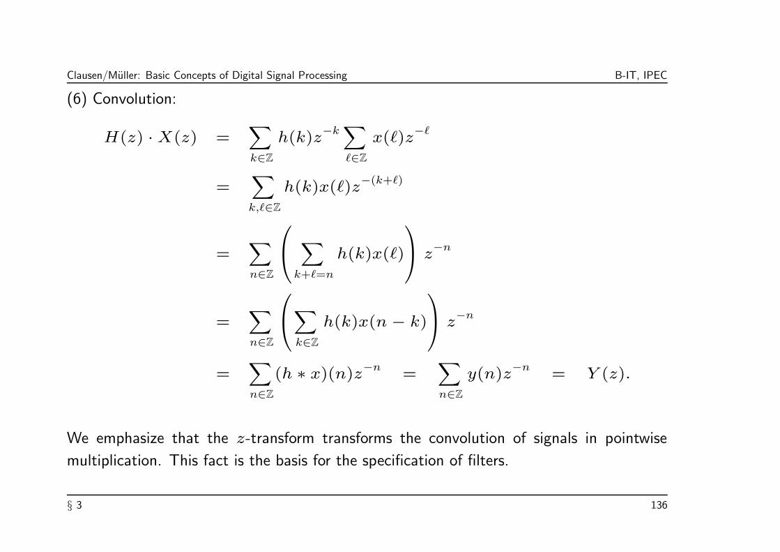
Clausen/Muller: Basic Concepts of Digital Signal Processing B-IT, IPEC
(6) Convolution:
H(z) ·X(z) =∑
k∈Z
h(k)z−k∑
`∈Z
x(`)z−`
=∑
k,`∈Z
h(k)x(`)z−(k+`)
=∑
n∈Z
∑
k+`=n
h(k)x(`)
z
−n
=∑
n∈Z
∑
k∈Z
h(k)x(n− k)
z
−n
=∑
n∈Z
(h ∗ x)(n)z−n
=∑
n∈Z
y(n)z−n
= Y (z).
We emphasize that the z-transform transforms the convolution of signals in pointwise
multiplication. This fact is the basis for the specification of filters.
§ 3 136

Clausen/Muller: Basic Concepts of Digital Signal Processing B-IT, IPEC
Similar to Definition 3.30 one has in the theory of filters another expression for the
z-transform.
Definition 3.46. Let T be a BIBO-stable LTI system with impulse response h = T [δ] ∈`1(Z). Then the z-transform
H(z) :=∑
n∈Z
h(n)z−n
is called transfer function of T (or h). One also speaks of the z-domain of T (or h).
§ 3 137

Clausen/Muller: Basic Concepts of Digital Signal Processing B-IT, IPEC
3.5 Convolution for CT-Signals
Just as the analogy between the CT-signal spaces Lp(R) and the DT-signal spaces `p(Z)
there is also a similar analogy between filtering in the CT-case and in the DT-case.
For example, the convolution of CT-signals can be defined in a similar fashion as for
DT-signals (see Section 3.2). This is no coincidence, since convolution can be generally
defined for so called locally compact groups G with a Haar measure. The convolution for
CT-signals (G = R) and for DT-signals (G = Z) can then be considered as special cases
of this more general concept.
In this section we give the main definitions and summarize some important properties of
the continuous convolution.
Definition 3.47. For continuous-time signals f, g: R → C the convolution of f and g at
t ∈ R is defined to be
(f ∗ g)(t) :=
∫ ∞
−∞f(s)g(t− s)ds.
§ 3 138

Clausen/Muller: Basic Concepts of Digital Signal Processing B-IT, IPEC
Attention: f ∗ g does in general not exist! The next theorem gives some conditions on
f and g which guarantees the the existence of f ∗ g. (One compare this theorem with
Theorem 3.13.)
Theorem 3.48. Let 1 ≤ p, q ≤ ∞, then the following properties hold.
(1) Let f, g, h : R → C, such that all convolution integrals in question exist. Then
f ∗ (g + h) = f ∗ g + f ∗ h, f ∗ g = g ∗ f and (f ∗ g) ∗ h = f ∗ (g ∗ h).Furthermore holds (λf) ∗ g = f ∗ (λg) = λ(x ∗ g) for arbitrary λ ∈ C.
(2) (Young Inequality) L1 ∗ Lp ⊆ Lp, i.e., for all f ∈ L1(R), g ∈ Lp(R) holds
f ∗ g ∈ Lp(R) and
||f ∗ g||p ≤ ||f ||1 · ||g||p.
§ 3 139

Clausen/Muller: Basic Concepts of Digital Signal Processing B-IT, IPEC
(3) Let p and q be conjugate exponents. Then for all f ∈ Lp and g ∈ Lq holds
f · g ∈ L1
and ||f · g||1 ≤ ||f ||p · ||g||qf ∗ g ∈ L
∞and ||f ∗ g||∞ ≤ ||f ||p · ||g||q.
(4) For all f ∈ Lp(R) and g ∈ L∞(R) one has f · g in Lp(R) and
||f · g||p ≤ ||f ||p · ||g||∞.
For a proof we refer to [Folland]. Also in the CT-case the convolution of two functions
transforms under the Fourier transform in pointwise multiplication (compare with Theorem
3.15).
Theorem 3.49. Let f, g ∈ L2(R), then f ∗ g ∈ L2(R) and
f ∗ g = f · g.
§ 3 140

Clausen/Muller: Basic Concepts of Digital Signal Processing B-IT, IPEC
3.6 Summary and Examples
In this chapter we have introduced a general system as a function between signal
spaces. Imposing properties such as linearity, time-invariance, and stability lead us to
stable LTI systems. One major result was formulated in Theorem 3.20: a stable LTI
system T can be expressed as convolution operator Ch w.r.t. the impulse response
h = T [δ] ∈ `1(Z) and, vice versa, each sequence h ∈ `1(Z) defines a stable LTI system
via convolution. Therefore, we often simply speak of a filter h and mean its associated
convolution operator Ch.
In Definition 3.21 we distinguished the cases where the impulse response h is of finite
length or infinite length. In the first case we called h an FIR filter and in the second case
an IIR filter.
§ 3 141
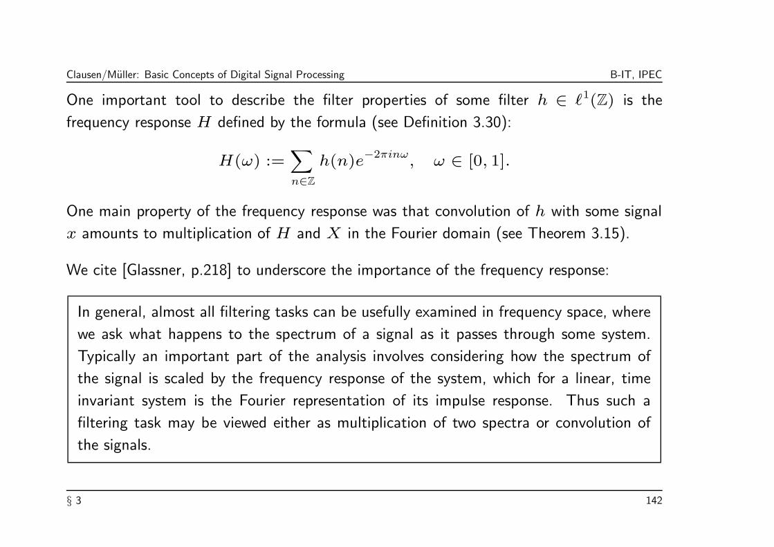
Clausen/Muller: Basic Concepts of Digital Signal Processing B-IT, IPEC
One important tool to describe the filter properties of some filter h ∈ `1(Z) is the
frequency response H defined by the formula (see Definition 3.30):
H(ω) :=∑
n∈Z
h(n)e−2πinω
, ω ∈ [0, 1].
One main property of the frequency response was that convolution of h with some signal
x amounts to multiplication of H and X in the Fourier domain (see Theorem 3.15).
We cite [Glassner, p.218] to underscore the importance of the frequency response:
In general, almost all filtering tasks can be usefully examined in frequency space, where
we ask what happens to the spectrum of a signal as it passes through some system.
Typically an important part of the analysis involves considering how the spectrum of
the signal is scaled by the frequency response of the system, which for a linear, time
invariant system is the Fourier representation of its impulse response. Thus such a
filtering task may be viewed either as multiplication of two spectra or convolution of
the signals.
§ 3 142

Clausen/Muller: Basic Concepts of Digital Signal Processing B-IT, IPEC
Depending on the properties of the magnitude response we have in Definition 3.36
considered three types of filters: lowpass, highpass, and bandpass filters.
In 5 we will describe further filter characteristics and give some methods of how to
construct FIR filters which approximate the ideal filters mentioned above. We conclude
this chapter with two examples which illustrates the introduced notions.
3.6.1 Haar filter
We start with an easy example and consider a pair of FIR filters h and g defined by
h(n) =
12 if n = 0, 1,
0 elsewhereand g(n) =
12 if n = 0,
−12 if n = 1,
0 elsewhere.
These filters play a crucial role in the Haar wavelet transform as we will see in Chapter ??.
§ 3 143

Clausen/Muller: Basic Concepts of Digital Signal Processing B-IT, IPEC
Their frequency response can easily be computed:
H(ω) =1
2+
1
2e−2πiω
= e−πiω · 1
2(eπiω
+ e−πiω
) = e−πiω
cos(πω)
and
G(ω) =1
2− 1
2e−2πiω
= e−πiω · 1
2(eπiω − e
−πiω) = e
−πiω · i · sin(πω).
§ 3 144

Clausen/Muller: Basic Concepts of Digital Signal Processing B-IT, IPEC
The magnitude response and phase response of h and g are shown in the following figure.
−2 −1 0 1 2 3−1
−0.5
0
0.5
1Filter coefficients of h
0 0.5 10
0.2
0.4
0.6
0.8
1
Magnitude response |H|
0 0.5 1−3
0
3
Phase response Φh
−2 −1 0 1 2 3−1
−0.5
0
0.5
1
Index n
Filter coefficients of g
0 0.5 10
0.2
0.4
0.6
0.8
1
Frequency ω
Magnitude response |G|
0 0.5 1−3
0
3
Frequency ω
Phase response Φg
§ 3 145

Clausen/Muller: Basic Concepts of Digital Signal Processing B-IT, IPEC
Note 3.50. The filters h and g have the following properties:
(1) The frequency response H is a modulation of a cosine-function. Similar G is, up to
the factor i, a modulation of a sine-function.
(2) |H| is in the interval [0, 12] monotonously decreasing with H(0) = 1 and H(1
2) = 0.
Hence, in some sense, H can be regarded as a lowpass filter. The quality, however, is
very poor.
(3) Similarly |G| is in the interval [0, 12] monotonously increasing with G(0) = 0 and
H(12) = 1. Hence, G can be regarded as highpass filter.
(4) The filters h and g constitute a so-called pair of associated filters. For a signal x,
the filtered signal h ∗ x contains the “low-frequency content” of x, whereas g ∗ xcontains the “high-frequency content” of x.
(5) The filters h an g considered as elements in `2(Z) are orthogonal.
(6) The filters h and g form the core of a so-called 2-band multirate filter bank.
§ 3 146
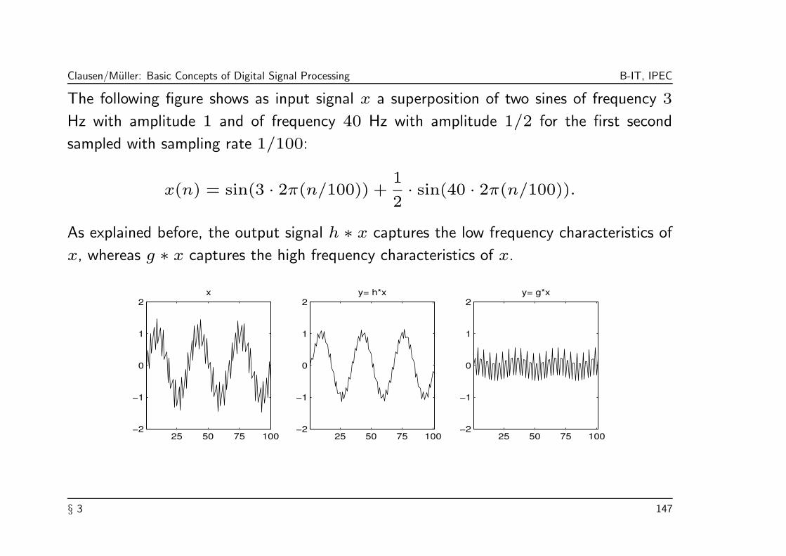
Clausen/Muller: Basic Concepts of Digital Signal Processing B-IT, IPEC
The following figure shows as input signal x a superposition of two sines of frequency 3
Hz with amplitude 1 and of frequency 40 Hz with amplitude 1/2 for the first second
sampled with sampling rate 1/100:
x(n) = sin(3 · 2π(n/100)) +1
2· sin(40 · 2π(n/100)).
As explained before, the output signal h ∗ x captures the low frequency characteristics of
x, whereas g ∗ x captures the high frequency characteristics of x.
25 50 75 100−2
−1
0
1
2x
25 50 75 100−2
−1
0
1
2y= h*x
25 50 75 100−2
−1
0
1
2y= g*x
§ 3 147

Clausen/Muller: Basic Concepts of Digital Signal Processing B-IT, IPEC
3.6.2 Averaging Filter
The averaging filters hN of length N is defined by
hN(n) =
1N if 0 ≤ n ≤ N − 1
0 elsewhere.
Hence the Haar lowpass filter of the last section is the averaging filter of length 2. The
frequency response can easily be computed by using the geometric series:
H(ω) =
N−1∑
n=0
1
Ne−2πiωn
=1
N
1 − e−2πiωN
1 − e−2πiω
=1
N
e2πiωN/2 − e−2πiωN/2
e2πiω/2 − e−2πiω/2· e
−2πiωN/2
e−2πiω/2
=1
N
sin(πωN)
sin(πωω)e−2πi(N−1)ω/2
§ 3 148
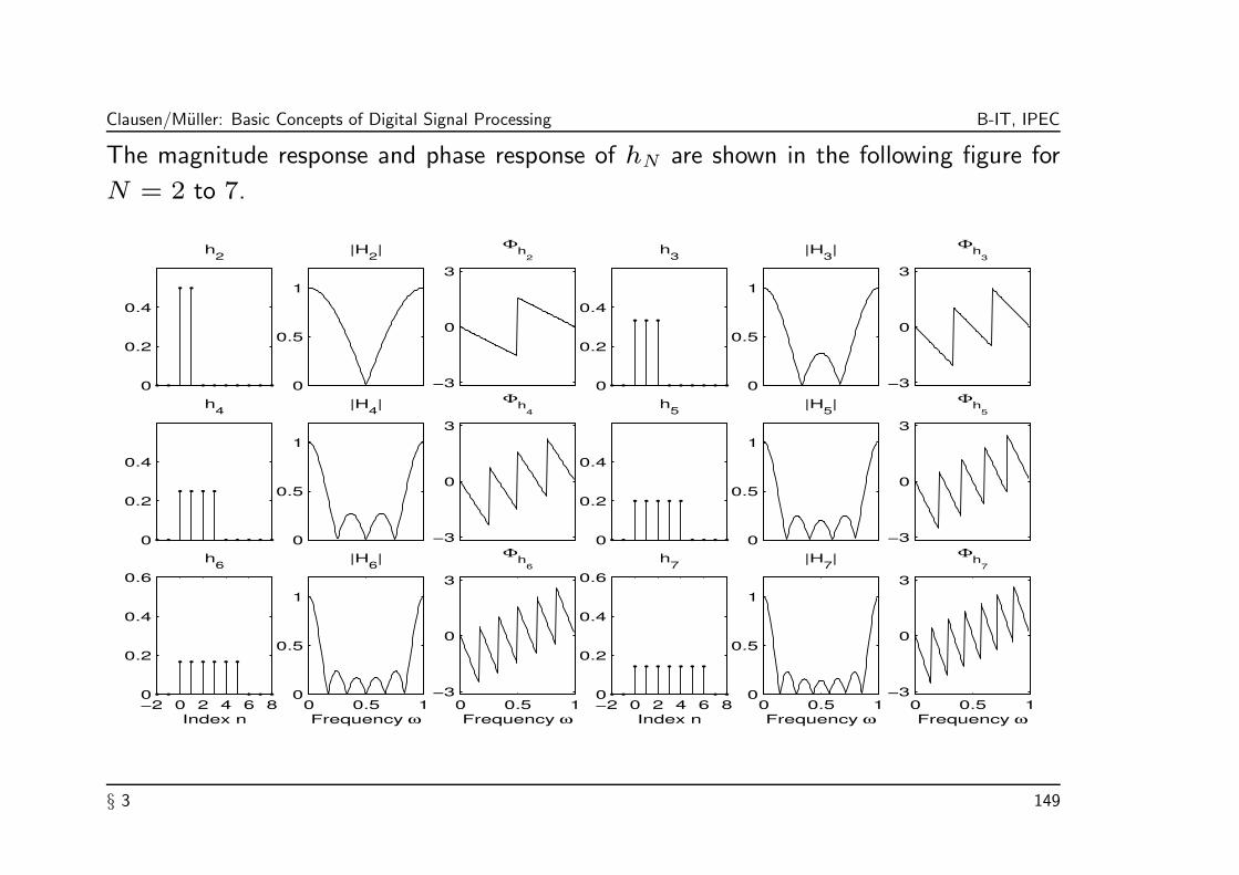
Clausen/Muller: Basic Concepts of Digital Signal Processing B-IT, IPEC
The magnitude response and phase response of hN are shown in the following figure for
N = 2 to 7.
0
0.2
0.4
h2
0
0.5
1
|H2|
−3
0
3
Φh
2
0
0.2
0.4
h3
0
0.5
1
|H3|
−3
0
3
Φh
3
0
0.2
0.4
h4
0
0.5
1
|H4|
−3
0
3
Φh
4
0
0.2
0.4
h5
0
0.5
1
|H5|
−3
0
3
Φh
5
−2 0 2 4 6 80
0.2
0.4
0.6
Index n
h6
0 0.5 10
0.5
1
Frequency ω
|H6|
0 0.5 1−3
0
3
Frequency ω
Φh
6
−2 0 2 4 6 80
0.2
0.4
0.6
Index n
h7
0 0.5 10
0.5
1
Frequency ω
|H7|
0 0.5 1−3
0
3
Frequency ω
Φh
7
§ 3 149

Clausen/Muller: Basic Concepts of Digital Signal Processing B-IT, IPEC
The following figure shows as an input signal x and for output signal y = h ∗ x filtered
with h = h5, h10, h20, and h40, respectively.
50 100 150 200 250 300 350 400 450 500
−2
0
2
x
50 100 150 200 250 300 350 400 450 500
−2
0
2
y=h 5*x
50 100 150 200 250 300 350 400 450 500
−2
0
2
y=h 10
*x
50 100 150 200 250 300 350 400 450 500
−2
0
2
y=h 20
*x
50 100 150 200 250 300 350 400 450 500 550
−2
0
2
y=h 40
*x
§ 3 150

Clausen/Muller: Basic Concepts of Digital Signal Processing B-IT, IPEC
Note 3.51. The following observation are illustrated by the last two figures.
(1) The cut-off frequency of hN is given by ω0 = 1/N . However, the filter properties
are not very good. For example, the pass band is not flat but drops right away and the
stop band exhibits many ripples of large amplitude.
(2) The previous figure illustrates that with increasing N the filtered signal y = hN ∗ xreflects better and better the low-frequency content of x.
(3) The length of the output signal y = h ∗ x does not only depend on the length of
the input signal x but also on the length of the filter length N of the FIR filter h. For
example, in our example the signal length of x is 512 and the length of the filtered
signal y = h40 ∗ x is 551.
§ 3 151

Clausen/Muller: Basic Concepts of Digital Signal Processing B-IT, IPEC
Chapter 4: Sampling and Aliasing
Doing signal processing with a computer one can, for example, store and process only a
finite number of parameters. Therefore, a continuous-time signal has, in general, to be
approximated in order to describe the approximation by a finite number of parameters.
Mathematically, this corresponds to a projection of the signal onto a finite-dimensional
vector space, which is the linear hull of a finite set of so-called synthesis functions. For
example, the discrete set of parameters could be
• the Fourier coefficients (for periodic signals),
• the coefficients of polynomials (when representing a function by its Taylor series), or
• the values of a CT-signal on a finite number of points in time.
§ 4 152

Clausen/Muller: Basic Concepts of Digital Signal Processing B-IT, IPEC
The third method, also referred to as sampling, is the easiest and most common way
to discretize a CT-signal. However, when sampling a signal one looses, in general,
information. This can lead to strong artefacts and distortions — also known as aliasing —
when reconstruction a CT-signal from the sampled version. In this chapter we
• give a strict definition of sampling,
• discuss conditions on the CT-signals which are sufficient for a perfect reconstruction of
the signal from the sampled version,
• desribe the aliasing effects, and
• discuss some methods to soften the resulting aretefacts and distortions.
§ 4 153

Clausen/Muller: Basic Concepts of Digital Signal Processing B-IT, IPEC
4.1 Sampling
Definition 4.1. In the following we summarize the basic definitions and notions.
(1) The procedure to generate a DT-signal by taking the values of a CT-signal on a
discrete set of points (in time) is referred to as sampling.
(2) The values of the DT-signal are then called samples, the points are called
sample points.
(3) In case any two neighboring sample points have the same distance T > 0
(equidistant), on also speaks of T -sampling. Then a CT-signal f : R → C transforms
into the DT-signal x: Z → C with
x(n) := f(T · n).
(4) For T -sampling, the number of samples per time unit is 1T which is referred to as
sampling rate. The sampling rate is measured in unit Hertz or simply hz.
§ 4 154

Clausen/Muller: Basic Concepts of Digital Signal Processing B-IT, IPEC
The transition from a CT-signal f : R → C to a sampled DT-signal x : Z → C results,
in general, in a loss of information, i.e., f cannot be reconstructed from x. At least,
one can try to reconstruct an approximation of f . This is done be using so-called
synthesis functions. For example, in case of T -sampling one can choose the characteristic
functions 1[tk,tk+1)(t) of the intervals [tk, tk+1), tk := T · k, between two neighboring
sample points. The one gets the function fT defined by
fT (t) :=
∞∑
k=−∞x(k)1[tk,tk+1)(t) =
∞∑
k=−∞f(T · k)1[tk,tk+1)(t).
In this case f is approximated by fT , i.e., the value f(t) is approximated by the constant
f(tk) where tk is the closest sampling point on the left of t.
§ 4 155

Clausen/Muller: Basic Concepts of Digital Signal Processing B-IT, IPEC
Of course, synthesis functions are not uniquely determined. For example, instead of the
characteristic functions one could also pick spline functions or trigonometric functions.
Hence, the quality of the approximation depends not only on the number and quality of
the sample values but also on the choice the synthesis function. However, there is no
canonical choice. The “right” choice depends very much on the class of CT-signals under
consideration and the application in mind.
For a certain class of CT-signals the choice of the so-called sinc-functions lead to a perfect
reconstruction of the CT-signal from its samples. This amazing property is the content of
the next section.
§ 4 156

Clausen/Muller: Basic Concepts of Digital Signal Processing B-IT, IPEC
4.2 Shannon Sampling Theorem
The Fourier transform f of a continuous-time signal f ∈ L1(R) exhibits the spectral
information on the signal. Intuitively, the value |f(ω)| expresses the intensity in which
the frequency ω ∈ R is “contained” in the signal f . Sometimes it suffices to consider
signals which only contain a certain range of frequencies.
For example, the human auditory system only recognizes frequencies which are below a
certain threshold (around 20 kHz). Therefore, for a given audio signal wiping out all
frequencies above this threshold results in a signal with no audible loss — at least for the
human ear. (A bat, however, would probably protest against such an intervention.)
§ 4 157

Clausen/Muller: Basic Concepts of Digital Signal Processing B-IT, IPEC
This is a good point for an excursion into the world of bats — creatures which
make up one quarter of the world’s mammal species. On Jim’s Bat Page
(http://www.jimlev.warc.org.uk/bats.htm#bat1) one finds the following nice
account on echolocation.
Echolocation of bats
Bats find their way around in the dark and locate food by calling out and listening
for echoes from nearby objects. In this way bats can detect such things as trees,
buildings, the ground, telephone wires and flying insects. The echolocation systems of
bats enable them to navigate, also to detect and home in on prey. In flight they are
able to avoid obstacles and other bats. They are able to determine the type, location,
direction and speed of their prey from the echoes they receive. An almost immediate
echo will be received from a nearby object and it will be relatively loud. The echoes
from further objects will be quieter and will take longer to return.
The sounds sent out by bats are very much higher in frequency than those that can be
detected by humans. We can hear sounds in the frequency range 20 Hz to 20, 000 kHz
whilst bats operate between 20 kHz and 150 kHz. This is known as ultrasonic sound.
§ 4 158

Clausen/Muller: Basic Concepts of Digital Signal Processing B-IT, IPEC
Typically, Pipistrelles use 40 − 50 kHz and Horseshoes use 80 − 100 kHz. Bat calls
are very complex. They may have several different frequencies or notes, and vary in
loudness.
The speed of sound through air is fairly constant and is equal to the frequency of the
sound multiplied by its wavelength. This means that if the frequency goes up, the
wavelength goes down. If the speed of sound is about 0.3 kilometers per second,
a 20 kHz sound has a wavelength of about 0.015 meters or 15 mm. A sound at
150 kHz has a wavelength of about 2 mm. This wavelength range between about
2 mm and 15 mm is also the approximate range of sizes of the insects they eat. The
shorter the wavelength (or the higher frequency) used by the bats then the smaller the
prey that can be detected. The shorter wavelengths give more accuracy in homing in
on prey.
The loudness of the ultrasonic pulses also changes depending on whether the bat is
searching for prey or capturing it. It is loudest during search becoming quieter during
capture.
§ 4 159

Clausen/Muller: Basic Concepts of Digital Signal Processing B-IT, IPEC
One would expect that the bats would fly around using the highest frequency so
that they could navigate and avoid obstacles with greatest accuracy. Unfortunately
the highest frequencies do not travel far compared with the lower frequencies (longer
wavelengths). For this reason bats use different frequencies for different purposes.
They use the lowest frequencies for travelling and searching for prey, changing to
higher frequencies to home in as the distance to the prey shortens, then the highest
frequencies at short range to contact and seize the prey. The sounds sent out by
bats usually consist of a series of pulses of ultrasound which sweep down from a high
frequency to a low frequency over a few thousands of a second. The time space
between the pulses allows any echo to return and to be processed in the brain of the
bat to give it information about its surroundings, and any prey that may be in range.
Some bats use pulses which do not change in frequency. It has been shown that these
bats detect frequency changes in the echoes due to either their own movement, or the
movement of their prey, or both. The frequency change is due to what is known as
Doppler shift. This is the effect that occurs when a police car with its siren wailing
§ 4 160
Clausen/Muller: Basic Concepts of Digital Signal Processing B-IT, IPEC
passes you. The frequency of the sound you hear drops as the car passes you. It is
higher as it approaches you and lower as it speeds away from you. The amount of shift
in frequency depends on the speed of the car - the higher the speed then the greater
the Doppler shift. If the car was stationary and you ran past it fast enough you would
also hear a Doppler shift due to your motion. The frequency shift that a bat detects is
a combination of the relative speeds and directions if itself and its prey.
Humans see by building up a picture in the brain from light reflected from surrounding
objects entering the eye. The bat brain builds up a similar picture from reflected sound.
In the case of a bat, the sound is arriving in pulses and the sound fed to the brain must
be a bit like the flashing light that we see at a disco. Just as our brains can make
out something of the inside of the disco and see the dancers, the bats brain can build
up a picture of its surroundings and nearby prey from the sound pulses it receives. In
addition, from the nature of the echoes receive, the bat is able to determine what sort
of prey it is seeing. For example, from the Doppler shift and the changes in loudness
of the echoes due to pulses reflected from insect wings the bat can detect the speed
that the insect is flapping its wings and deduce the size of the prey.
§ 4 161

Clausen/Muller: Basic Concepts of Digital Signal Processing B-IT, IPEC
Small insects flap faster than large ones, for example, mosquitoes beat their wings
more than 200 times a second whereas larger insects such as moths and large beetles
may only beat about 50 times a second.
Larger bats generally use lower frequency ranges than smaller bats. This means that
they can see further than smaller bats but do not see the smallest insects, - which they
would find it hard to catch anyway.
The echolocation methods used by bats are good enough to allow capture of the prey
in the bat’s mouth most of the time. For near misses, the wing tips and tail are used
to scoop up the prey.
For further readings Jim refers to “Bats” by Phil Richardson published by Whittet Books
(ISBN 0-905483-41-3) and “The Natural History of Hibernating Bats” by Roger Ransom
published by Christopher Helm (ISBN 0-7470-2802-8).
§ 4 162

Clausen/Muller: Basic Concepts of Digital Signal Processing B-IT, IPEC
Signals which contain only frequencies up to a certain threshold are called bandlimited.
We give a more rigorous definition.
Definition 4.2. Let Ω > 0. The CT-signal f ∈ L2(R) is called Ω-bandlimited if the
Fourier transform f vanishes for |ω| > Ω:
f(ω) = 0 ∀|ω| > Ω, i.e., suppf ⊂ [−Ω,Ω].
The following figure shows a Fourier transform f of an Ω-bandlimited function f .
−Ω Ω
§ 4 163
Clausen/Muller: Basic Concepts of Digital Signal Processing B-IT, IPEC
Bandlimited functions have surprising properties. For example, a continuous-time function
f ∈ L2(R) may be, in general, discontinuous or even undefined at some points. If f is
Ω-bandlimited, however, the following theorems hold:
Theorem 4.3. If f ∈ L2(R) is bandlimited then f is smooth (i.e., infinitely often
differentiable).
Note 4.4. As mentioned in Note 1.35 f ∈ L2(R) denotes actually a whole class of
functions. Therefore, to be more precise, Theorem 4.3 should read that in case f is
bandlimited there is a smooth function equivalent to f . Only for this smooth (and hence
continuous) representative it is possible to take samples.
§ 4 164

Clausen/Muller: Basic Concepts of Digital Signal Processing B-IT, IPEC
The smaller Ω, i.e., the smaller the range of frequency contained in the signal, the
smoother the signal. In other words, local bursts and discontinuity points in the signal
result in high frequency components in the Fourier spectrum.
One other fact about bandlimited function, often referred to as uncertainty principle, is
important in view of applications.
Theorem 4.5. If f ∈ L2(R) is bandlimited then f cannot be compactly supported.
Therefore, in real-world applications, when one has to deal with time-limited signals one
cannot simply assume that f is bandlimited and has to struggle with the consequences
which are known as aliasing.
§ 4 165

Clausen/Muller: Basic Concepts of Digital Signal Processing B-IT, IPEC
The sampling theorem by Shannon says that a bandlimited function f can be reconstructed
perfectly from a suitable equidistant set of samples.
Theorem 4.6. [Shannon.] 1 Let f ∈ L2(R) be an Ω-bandlimited function and let x
be the T -sampled version of f with T := 12Ω, i.e., x(n) = f(nT ), n ∈ Z. Then f
can be reconstructed from x:
f(t) =
∞∑
n=−∞x(n)sinc
(t− nT
T
)=
∞∑
n=−∞f
(n
2Ω
)sinc (2Ωt− n) ,
where the scaled and translated versions of the sinc-function
sinc (x) :=
sinπxπx x 6= 0
1 x = 0.
are used as synthesis function.
1Shannon(1949), Kotel’nikov(1933), Whittaker(1915), de la Vallee Poissin(1908)
§ 4 166
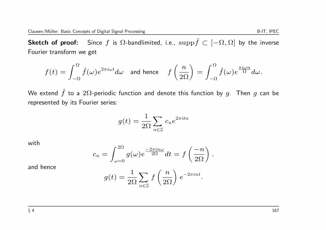
Clausen/Muller: Basic Concepts of Digital Signal Processing B-IT, IPEC
Sketch of proof: Since f is Ω-bandlimited, i.e., suppf ⊂ [−Ω,Ω] by the inverse
Fourier transform we get
f(t) =
∫ Ω
−Ω
f(ω)e2πiωt
dω and hence f
(n
2Ω
)=
∫ Ω
−Ω
f(ω)eπiωn
Ω dω.
We extend f to a 2Ω-periodic function and denote this function by g. Then g can be
represented by its Fourier series:
g(t) =1
2Ω
∑
n∈Z
cne2πitn
with
cn =
∫ 2Ω
ω=0
g(ω)e−2πinω
2Ω dt = f
(−n2Ω
).
and hence
g(t) =1
2Ω
∑
n∈Z
f
(n
2Ω
)e−2πint
.
§ 4 167

Clausen/Muller: Basic Concepts of Digital Signal Processing B-IT, IPEC
From this we get
f(t) =
∫ Ω
−Ω
g(ω)e2πiωt
dω
=1
2Ω
∫ Ω
−Ω
∑
n∈Z
f
(n
2Ω
)e−2πinω
e2πiωt
dω
=∑
n∈Z
f
(n
2Ω
)1
2Ω
∫ Ω
−Ω
e2πiω(t−n)
dω
︸ ︷︷ ︸=sinc (2Ωt−n))
.
§ 4 168
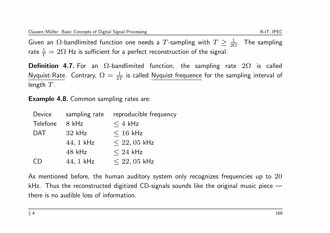
Clausen/Muller: Basic Concepts of Digital Signal Processing B-IT, IPEC
Given an Ω-bandlimited function one needs a T -sampling with T ≥ 12Ω. The sampling
rate 1T = 2Ω Hz is sufficient for a perfect reconstruction of the signal.
Definition 4.7. For an Ω-bandlimited function, the sampling rate 2Ω is called
Nyquist-Rate. Contrary, Ω = 12T is called Nyquist frequence for the sampling interval of
length T .
Example 4.8. Common sampling rates are:
Device sampling rate reproducible frequency
Telefone 8 kHz ≤ 4 kHz
DAT 32 kHz ≤ 16 kHz
44, 1 kHz ≤ 22, 05 kHz
48 kHz ≤ 24 kHz
CD 44, 1 kHz ≤ 22, 05 kHz
As mentioned before, the human auditory system only recognizes frequencies up to 20
kHz. Thus the reconstructed digitized CD-signals sounds like the original music piece —
there is no audible loss of information.
§ 4 169
Clausen/Muller: Basic Concepts of Digital Signal Processing B-IT, IPEC
4.3 Aliasing
Ken C. Pohlmann gives in his book “Principles of Digital Audio” [Pohlmann] the following
general description of the aliasing problem:
One particular challenge to a digital audio system designer is that of aliasing, a kind
of sampling confusion that can occur in the recording side of the signal chain. Just as
a criminal can take many names and thus confuse identity, aliasing can create false
signal components. These erroneous signals can appear within the audio bandwidth
and are impossible to distinguish from legitimate signals. Obviously, it is the designer’s
obligation to prevent such distortion from ever occurring. In practice, aliasing is not a
limitation. It merely underscores the importance of observing the criteria of sampling
theory.
§ 4 170

Clausen/Muller: Basic Concepts of Digital Signal Processing B-IT, IPEC
From an image processing point of view Andrew S. Glassner writes in [Glassner]:
One way to make sure our pictures are as good as they can be is to make sure that
they contain nothing extraneous or wrong. This sounds fine in principle, but it turns
out that the mere process of representing an inherently continuous color picture on a
device with a finite number of spatial locations usually introduces errors of its own.
These errors are known collectively as aliasing, and they lead to phenomena like jagged
edges, thin objects that seem to be broken into pieces, and, in animations, objects that
suddenly appear and disappear.
§ 4 171
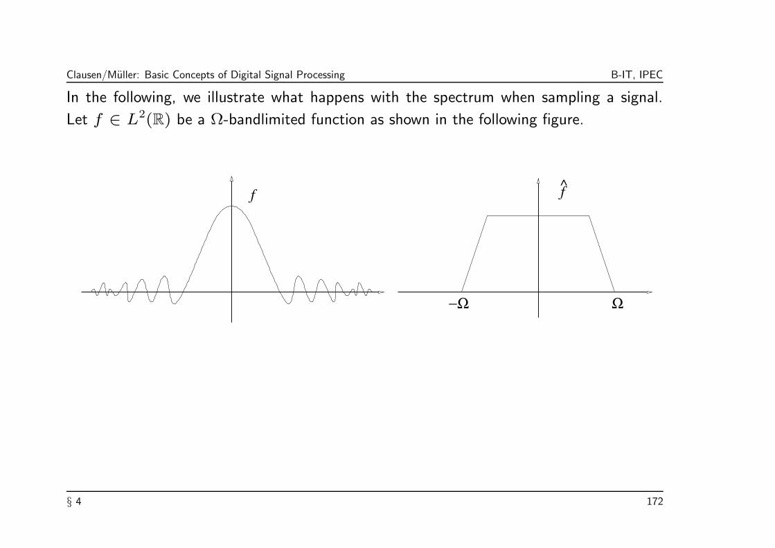
Clausen/Muller: Basic Concepts of Digital Signal Processing B-IT, IPEC
In the following, we illustrate what happens with the spectrum when sampling a signal.
Let f ∈ L2(R) be a Ω-bandlimited function as shown in the following figure.
ff
−Ω Ω
§ 4 172

Clausen/Muller: Basic Concepts of Digital Signal Processing B-IT, IPEC
Let x : Z → C be the DT-signal by sampling f with a sampling rate 1T , i.e.,
x(n) = f(nT ), n ∈ Z.
Then the spectrum x of x is the 1-periodization of a scaled version of the spectrum f .
The precise statement is formulated in the next theorem.
Theorem 4.9. Let f be a continuous function with f ∈ L2(R) and x be the DT-signal
obtained from f by T -sampling, i.e., x(n) = f(nT ) for n ∈ N. Then
x(ω) =1
T
∑
k∈Z
f
(ω + k
T
).
§ 4 173

Clausen/Muller: Basic Concepts of Digital Signal Processing B-IT, IPEC
Proof: We first proof the result for the case T = 1. Let
g(ω) :=∑
k∈Z
f(ω + k),
ω ∈ R. To show that x = g it suffices to show that the inverse Fourier transform of g
and x coincide, i.e., x = g. To this means we compute the nth Fourier coefficient of g:
∫ 1
0
g(ω)e2πiωn
dω =
∫ 1
0
∑
k∈Z
f(ω + k)e2πiωn
dω
=∑
k∈Z
∫ k+1
k
f(ω)e2πi(ω−k)n
dω
=
∫
R
f(ω)e2πiωn
dω
= f(n) = x(n).
For general T > 0 we consider the function h defined by h(t) := f(t · T ) instead of f
in the above proof. Then the general case follows by using rule (5) of Theorem 2.9.
§ 4 174

Clausen/Muller: Basic Concepts of Digital Signal Processing B-IT, IPEC
We now consider the three cases where the sampling rate 1T is equal to, above and below
the Nyquist rate 2Ω.
Case 1: T = 12Ω
When the sampling rate equals the Nyquist rate, the Fourier transform of f can be
recovered from x since
f(ω) = χ[−1/2T,1/2T ] · T · x(Tω) = χ[−Ω,Ω] · T · x(Tω)
Therefore, f can be perfectly recovered from x by taking the inverse Fourier transform of
χ[−Ω,Ω] · T · x(T ·). Actually, this is just a reformulation of Shannon’s sampling theorem.
1/2 1/2
x
§ 4 175

Clausen/Muller: Basic Concepts of Digital Signal Processing B-IT, IPEC
Case 2: T < 12Ω
In this case the sampling rate 1T is above the Nyquist rate 2Ω. One then also speaks
from oversampling. As in Case 1, f can be recovered from x and f can be perfectly
reconstructed from x.
x
One can show that in the case of oversampling, increasing the sampling
rate leads to faster convergence properties of the reconstruction series f(t) =∑∞n=−∞ x(n)sinc
(1T (t− nT )
).
§ 4 176
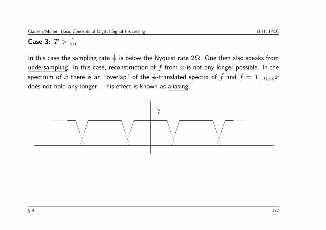
Clausen/Muller: Basic Concepts of Digital Signal Processing B-IT, IPEC
Case 3: T > 12Ω
In this case the sampling rate 1T is below the Nyquist rate 2Ω. One then also speaks from
undersampling. In this case, reconstruction of f from x is not any longer possible. In the
spectrum of x there is an “overlap” of the 1T -translated spectra of f and f = 1[−Ω,Ω]x
does not hold any longer. This effect is known as aliasing.
x
§ 4 177

Clausen/Muller: Basic Concepts of Digital Signal Processing B-IT, IPEC
We investigate the aliasing effect in a more rigorous way. Let T = 1Ω be a sampling rate
for some Ω > 0 and f ∈ L2(R) only be an Ω′-bandlimited function for some Ω′ with
Ω < Ω′< 3Ω.
Then T -sampling of f leads to the undersampled DT-signal x with x(k) := f(kT ). By
the Fourier inversion holds
f(kT ) =
∫ Ω′
−Ω′f(ω)e
2πiωkTdω (as f = 0 for |ω| > Ω′)
=
∫ 3Ω
−3Ω
f(ω)e2πiωkT
dω
=
∫ −Ω
−3Ω
f(ω)e2πiωkT
dω +
∫ Ω
−Ω
f(ω)e2πiωkT
dω +
∫ 3Ω
Ω
f(ω)e2πiωkT
dω.
§ 4 178
Clausen/Muller: Basic Concepts of Digital Signal Processing B-IT, IPEC
By a suitable substitution and using e2πiωkT = e2πiω′kT for ω′ − ω ∈ Z one obtains
x(k) = f(kT ) =
∫ Ω
−Ω
(f(ω) + f(ω + 2Ω) + f(ω − 2Ω))︸ ︷︷ ︸=:(∗)
e2πiωkT
dω (3)
We define a function g via its Fourier transform:
g(ω) :=
(∗) if |ω| ≤ Ω
0 otherwise.
Then, g is Ω-bandlimited and by Equation (3) holds g(kT ) = f(kT ) for all k ∈ Z.
Conclusion: The reconstruction of the CT-signal from the undersampled DT-signal x (by
means of the sinc-synthesis functions of the Shannon Theorem 4.6) does not result in the
original signal f but in the signal g.
§ 4 179

Clausen/Muller: Basic Concepts of Digital Signal Processing B-IT, IPEC
g
f
−Ω
−Ω
Ω
Ω’ ’
As illustrated, in the spectrum of g high frequency above |Ω| are “fold” into the interval
[−Ω,Ω]. In other words, in the undersampled DT-signal x high frequency components
of f outside the interval [−Ω,Ω] cannot be distinguished from certain low frequency
components of f within [−Ω,Ω], i.e., high-frequency components take on the identity of
a lower frequency.
This effect is known as aliasing.
§ 4 180

Clausen/Muller: Basic Concepts of Digital Signal Processing B-IT, IPEC
4.4 Down- und Upsampling
In Example 3.4 and 3.5 we have already introduced the downsampler ↓M and upsampler
↑M defined by
(↓M)[x](n) := x(M · n) and (↑M)[x](n) =
x(n/M), if M |n,
0, otherwise.
for some M ∈ N, n ∈ Z. Down- und upsampler play a central role in digital signal
processing such as in the theory of multirate filterbanks — as we will see in a later chapter.
In this section we summarize some of the basic properties of the down- and upsampler and
discuss the problem which arise in connection with the aliasing effect.
In the following discussion, we restrict to the case M = 2 which already exhibits the
typical problems to cope with.
§ 4 181

Clausen/Muller: Basic Concepts of Digital Signal Processing B-IT, IPEC
As mentioned in Example 3.28 the down- and upsampler are linear, continuous, and
stable. The downsampler ↓M destroys information. One does have (↓M)(↑M) = I,
but (↑M)(↓M) 6= I.
A nice mathematical property is the fact that the sampling operators (↓2) and (↑2)are transposed maps with respect to the `2(Z)-inner product. In other words, for all
x, y ∈ `2(Z) holds
〈(↓2)x|y〉`2(Z) = 〈x|(↑2)y〉`2(Z).
§ 4 182

Clausen/Muller: Basic Concepts of Digital Signal Processing B-IT, IPEC
4.4.1 Sampling operators in the z-domain
Next we investigate the effects of the sampling operators in the z-domain. Note that
since (↑2) and (↓2) are not time invariant they are not representable as convolution
filter. Therefore, there is no z-transforms for (↑2) and (↓2). However, the effects on the
sampled signals can be studied in the z-domain.
Let x ∈ `1(Z) be the input signal, u := (↑2)[x] be the upsampled, and v := (↓2)[x]be the downsampled signal. Then the z-transforms X, V , and U , satisfy the following
relations:
§ 4 183

Clausen/Muller: Basic Concepts of Digital Signal Processing B-IT, IPEC
U(z) =∑
k∈Z
xkz−2k
= X(z2) (4)
V (z) =∑
k∈Z
x2kz−k
=1
2
∑
k∈Z
xk(z12)
−k+
1
2
∑
k∈Z
xk(−z12)
−k(5)
=1
2(X(z
12) +X(−z1
2)).
The operators (↓2) und (↑2), defined in the time domain, can also be defined in the
z-domain via (4) and (5). We use for these operators the same symbols (↓2) and (↑2)as in the time domain. With this convention holds, for example, (↓2)[x](n) = x(2 · n)
and ((↑2)X)(z) = X(z2).
§ 4 184

Clausen/Muller: Basic Concepts of Digital Signal Processing B-IT, IPEC
4.4.2 Sampling operators in the Fourier domain
By setting z = e2πiω in (4) and (5) we get the relations between x, u, and v in the
Fourier (also called spectral domain or ω-domain):
U(ω) = X(2ω) (6)
V (ω) =1
2(X(ω2) +X(ω2 + 1
2)) (7)
By downsampling with (↓2) one looses half of the data and, in general, also some
information. In the Fourier domain this loss of data appears as mixing of different
frequency components. As in the case of sampling CT-signals (see Section 3), the effect
is known as aliasing.
§ 4 185

Clausen/Muller: Basic Concepts of Digital Signal Processing B-IT, IPEC
The equation (7) says that the frequency component for ω2 and ω
2 + 12 of the signal x are
identified and summed up in the 2-downsampled signal v. This is illustrated in Figure 8.
X( )ω
-1 -1/2 1/2 1
ωV( )
ω-1 -1/2 1/2 1 ω
Figure 8: Downsampling in the frequency domain.
§ 4 186

Clausen/Muller: Basic Concepts of Digital Signal Processing B-IT, IPEC
Upsampling with (↑2) leads to the contrary effect, which is also known as imaging. Here
the frequency component at ω of the original signal x is responsible for two frequency
components at ω2 and ω
2 + 12 of the 2-upsampled signal u. Equation (6) says that the
frequency spectrum is compress by the factor of 2 (see Figure 9).
X( )ω
ω-1 -1/2 1/2 1
ω-1 -1/2 1/2 1
ωU( )
Figure 9: Upsampling in the frequency domain.
§ 4 187

Clausen/Muller: Basic Concepts of Digital Signal Processing B-IT, IPEC
Due to the aliasing effects, the original signal x cannot in general be perfectly reconstructed
from the downsampled signal v = (↓2)[x]. Similar to the CT-case some additional
condition on the spectrum of x also guarantees perfect reconstruction.
Definition 4.10. A DT-signal x is called bandlimited by some Ω ∈ [0, 12] if
X(ω) = 0 for Ω ≤ |ω| ≤ 12.
X( )ω
-1 -1/2 1/2 1 ω -1 -1/2 1/2 1
ωV( )
ω -1 -1/2 1/2 1 ω
ωW( )
Figure 10: No aliasing if x is bandlimited by Ω ≤ 14.
§ 4 188

Clausen/Muller: Basic Concepts of Digital Signal Processing B-IT, IPEC
If the signal x is bandlimited by Ω = 14 then there is no aliasing and x can be
reconstructed from v as follows (see also Figure 10):
(1) By (↑2)-upsampling one obtains the signal w := (↑2)v with Fourier transform
W (ω) =1
2(X(ω) +X(ω + 1
2)). (8)
(2) Cut off the frequencies in W in the Fourier domain which resulted from the
imaging-effect. This are all frequencies in
[−1
2,1
2
]\[−1
4,1
4
]
and all translates by an integer number.
(3) Multiply the result by a factor of 2, then one recovers the Fourier transform X of the
original signal x.
§ 4 189

Clausen/Muller: Basic Concepts of Digital Signal Processing B-IT, IPEC
Note 4.11. In the time domain the reconstruction of the original signal from an
downsampled version corresponds to an interpolation for the odd sample points of w
(at these points w is zero). Therefore, in this context one also speaks form an
interpolation filter which reconstructs the bandlimited signal x from w. Again the
mathematical background is based on some version of Shannon’s sampling theorem.
For a more detailed discussion we refer to Chapter 3 of [Strang/Nguyen].
§ 4 190

Clausen/Muller: Basic Concepts of Digital Signal Processing B-IT, IPEC
Chapter 5: FIR Filters
In this chapter we follow in most part Chapter 8 of [Proakis/Manolakis].
In the design of frequency-selective filters, the desired filter characteristics are specified
in the frequency domain in terms of the magnitude and the phase response. In the
filter design process, one determines the coefficients of an FIR or IIR filter that closely
approximates the desired frequency response specifications. The issue of which type of
filter to design, FIR or IIR, depends on the nature of the problem and on the specifications
of the desired frequency response.
There are many different theoretical methods for filter design which have been implemented
and incorporated in numerous computer software programs such as MatLab. These
programs allow the user to specify the desired filter characteristics and then computes the
filter that best fits the desired design requirements.
§ 5 191

Clausen/Muller: Basic Concepts of Digital Signal Processing B-IT, IPEC
This chapter allows us only to have a look at some aspects of filter design. We concentrate
on the following kind of filters.
(1) We assume our filters to be causal, since this requirement is decisive for the physically
realization of the filter.
(2) We only deal with FIR-filters, i.e., filters with a finite impulse response. Note that
any FIR filter can be made causal by shifting the filter coefficients suitably.
(3) We want to restrict ourselves to the case of linear-phase filters which is an important
property in view of applications. This property is equivalent to a certain symmetry or
asymmetry condition on the filter coefficients as we will see later.
§ 5 192
Clausen/Muller: Basic Concepts of Digital Signal Processing B-IT, IPEC
5.1 Causality and its Implications
We recall that a filter h is called causal if h(n) = 0 for n < 0. In this case the frequency
response is given by
H(ω) :=∞∑
n=0
h(n)e−2πinω
.
The Paley-Wiener Theorem gives necessary and sufficient conditions that a frequency
response H must satisfy in order for the resulting filter to be causal. One version of this
theorem can be stated as follows (see [Proakis/Manolakis, p. 616] ):
§ 5 193

Clausen/Muller: Basic Concepts of Digital Signal Processing B-IT, IPEC
Theorem 5.1 (Paley-Wiener). If the filter h ∈ `1(Z) is causal then
∫ 1
0
| log |H(ω)||dω < ∞.
Conversely, if |H| is square integrable and if the above integral is finite, then one can
associate with |H| a phase response Φ such that the resulting filter with frequency
response
H(ω) = |H(ω)| · eiΦh(ω)
is causal.
§ 5 194

Clausen/Muller: Basic Concepts of Digital Signal Processing B-IT, IPEC
The Paley-Wiener Theorem has some immediate consequences:
(1) For a causal filter h, the frequency response H cannot be zero except at a finite set
of points in frequency, since the integral in the Paley-Wiener Theorem then becomes
infinite. In particular, H cannot be zero over any finite band of frequencies.
(2) From (1) follows that there is no causal filter realizing an ideal lowpass, bandpass, or
highpass filter.
(3) Since any FIR filter can be made causal by a shift (which amounts to a modulation
in the frequency response and hence leaves the magnitude response unchanged), it
follows from (2) that there is no FIR filter realizing an ideal filter.
§ 5 195

Clausen/Muller: Basic Concepts of Digital Signal Processing B-IT, IPEC
5.2 The Ideal Lowpass Filter
We have just seen that an ideal lowpass filter with cut-off frequency ω0 as illustrated
below cannot be realized by a causal filter or FIR filter.
0
In the following, we investigate if there is at least a noncausal filter realizing the ideal
lowpass filter. This might give us some ideas of how to approximate the ideal filter by FIR
filters.
§ 5 196

Clausen/Muller: Basic Concepts of Digital Signal Processing B-IT, IPEC
The frequency response of an ideal lowpass filter with cut-off frequency ω0, 0 < ω0 ≤ 1/2,
and with real coefficients is symmetric and 1-periodic. Hence it is specified on [0, 1/2] by
the formula
Hω0(ω) :=
1 0 ≤ ω ≤ ω0
0 ω0 < ω ≤ 1/2
§ 5 197

Clausen/Muller: Basic Concepts of Digital Signal Processing B-IT, IPEC
We now want to know, if there is a filter h = (h(n))n∈Z with real coefficients whose
frequency response equals Hω0, i.e.,
H(ω) =∑
n∈Z
h(n)e−2πiωn
= Hω0(ω) = Hω0
(−ω)
for ω ∈ [0, 1]. From this we see that the filter coefficients h(n) must be the Fourier
coefficients of the Fourier series of Hω0, i.e.,
h(n) =
∫ 1
0
Hω0(ω)e
2πiωndω
=
∫ ω0
−ω0
e2πiωn
dω
= 2ω0sinc (2ω0n),
where the computation follows as in Example 2.16. In other words, the filter
corresponding to the ideal lowpass filter with cut-off frequency ω0 is the sinc-function
t 7→ 2ω0sinc (2ω0t) sampled at the integers n ∈ Z.
§ 5 198

Clausen/Muller: Basic Concepts of Digital Signal Processing B-IT, IPEC
The following figure shows the sinc-filter coefficients for the case ω0 = 1/8.
−20 −15 −10 −5 0 5 10 15 20−0.1
0
0.1
0.2
0.3
Index n
Sinc−filter with cut−off frequency ωO
=1/8
§ 5 199

Clausen/Muller: Basic Concepts of Digital Signal Processing B-IT, IPEC
However, as mentioned before, there are several problems with the sinc-filter coefficients:
(1) The sinc-filter is not causal.
(2) The sinc-filter is not an FIR filter.
(3) Even worse, the filter is not even stable. For example, for ω0 = 1/4 one can show
that the sequence (h(2n))n∈Z behaves, up to a constant, like the sequence (1/n)n∈Z
which is clearly not in `1(Z).
§ 5 200

Clausen/Muller: Basic Concepts of Digital Signal Processing B-IT, IPEC
5.3 Characteristics of Practical Frequency-Selective Filters
From our previous discussion follows that ideal filters are noncausal and hence physically
not realizable for real-time signal processing applications. When an ideal filter is converted
into a realizable FIR filter, the perfect behavior is degraded. For example, one can observe
the following phenomena:
• Causality implies that the frequency response H of the filter cannot be zero, except at
a finite set of points in the frequency domain. This leads to ripples in the passband
and stopband,
• In addition, H cannot have an infinitely sharp cutoff from passband to stopband, i.e.,
H cannot drop from unity to zero abruptly and each of the sharp discontinuities is
smeared into a range of frequencies.
§ 5 201

Clausen/Muller: Basic Concepts of Digital Signal Processing B-IT, IPEC
In applications some degradations in the fequency response may be tolerable. For example,
a small amount of ripples in the passband or in the stopband as shown in Figure 11 may
be acceptable.
1
2
1
Figure 11: Magnitude characteristics of physically realizable lowpass filters.
§ 5 202

Clausen/Muller: Basic Concepts of Digital Signal Processing B-IT, IPEC
The following filter characteristics are illustrated by Figure 11.
• The transition of the frequency response from passband to stopband defines the
transition band of the filter.
• The band-edge frequency ωp define the edge of the passband, while the frequency ωsdenotes the beginning of the stopband.
• The width of the transition band is ωs − ωp.
• The width of the passband is called bandwidth of the filter. For example, if the filter is
lowpass with a passband edge frequency ωp, its bandwidth is ωp.
• If there are ripples in the passband of the filter, its value is denoted as δ1, and the
magnitude |H| varies between the limits 1 ± δ1. The ripples in the stopband of the
filter is denoted as δ2.
To accommodate a large dynamic range in the graph of the magnitude response of a filter,
it is common practice to use the decibel-scale as introduced in Section 3. Consequently,
the ripples in the passband is 20 log10 δ1 decibels, and that in the stopband is 20 log10 δ2.
§ 5 203

Clausen/Muller: Basic Concepts of Digital Signal Processing B-IT, IPEC
To summarize, in any filter design problem we can specify
(1) the maximum tolerable passband ripples,
(2) the maximum tolerable stopband ripples,
(3) the passband edge frequency ωp, and
(4) the stopband edge frequency ωs.
Based on these specifications, one is now interested in the construction of a filter h whose
frequency response H best approximates these specifications. Of course, the degree to
which H approximates the specifications depends in part on the number of non-zero filter
coefficients.
§ 5 204

Clausen/Muller: Basic Concepts of Digital Signal Processing B-IT, IPEC
5.4 Linear-Phase FIR Filters
Let h be a causal FIR filter of length M . Then the transfer function of h is given by
H(z) =
M−1∑
k=0
h(k)z−k
which can be viewed as a polynomial of degree M − 1 in the variable z−1. By definition,
the zeros of the filter h are the roots of this polynomial.
An FIR filter h has linear phase if the filter coefficients satisfy the following symmetry or
antisymmetry conditions:
h(n) = ±h(M − 1 − n), n = 0, 1, . . . ,M − 1.
§ 5 205

Clausen/Muller: Basic Concepts of Digital Signal Processing B-IT, IPEC
From this follows that the transfer function of a causal, linear-phase FIR filter of length
M is of the form:
H(z) = z−(M−1)/2
h
(M − 1
2
)+
(M−3)/2∑
k=0
h(k)[z
(M−1−2k)/2 ± z−(M−1−2k)/2
]
if M is odd and
H(z) = z−(M−1)/2
(M/2)−1∑
k=0
h(k)[z
(M−1−2k)/2 ± z−(M−1−2k)/2
]
if M is even.
§ 5 206

Clausen/Muller: Basic Concepts of Digital Signal Processing B-IT, IPEC
Now, if we substitute z−1 for z in the transfer function of h and multiply both sides of
the resulting equation by z−(M−1), we obtain
z−(M−1)
H(z−1
) = ±H(z).
This result implies that the roots of the polynomial H(z) are identical to the roots of the
polynomial H(z−1). In other words, if z1 is a root of H(z), then 1/z1 is also a root.
Furthermore, since the filter coefficients h(k) are assumed to be real, complex-valued
roots must occur in complex-conjugate pairs. Hence, if z1 is a complex-valued root, z1 is
also a root. Therefore, 1/z1 must also be a root. The next figure illustrates the symmetry
that exists in the location of the zeros of a linear-phase FIR filter.
§ 5 207

Clausen/Muller: Basic Concepts of Digital Signal Processing B-IT, IPEC
The frequency response of a linear-phase FIR filters are obtained by evaluating the formulas
of the transfer function on the unit circle, i.e., by setting z = e2πiω. From the formulas
for H(z) one then derives the following formulas for H(ω). If h is symmetric then H(ω)
can be expressed as
H(ω) = Hr(ω)e−2πiω(M−1)/2
where Hr(ω) is a real function of ω and can be expressed as
Hr(ω) = h
(M − 1
2
)+ 2
(M−3)/2∑
k=0
h(k) cos 2πω
(M − 1
2− k
)
if M is odd and
Hr(ω) = 2
(M/2)−1∑
k=0
h(k) cos 2πω
(M − 1
2− k
)
if M is even. The antisymmetric case is similar and left as an exercise.
§ 5 208

Clausen/Muller: Basic Concepts of Digital Signal Processing B-IT, IPEC
The phase response of the filter for both M odd and M even is
Φh(ω) =
−ω(M − 1
2
), if Hr(ω) > 0,
−ω(M − 1
2
)+
1
2, if Hr(ω) < 0.
Note that, for a symmetric filter h, the number of filter coefficients that specify the
frequency response is (M + 1)/2 when M is odd or M/2 when M is even.
§ 5 209

Clausen/Muller: Basic Concepts of Digital Signal Processing B-IT, IPEC
5.5 Design of Linear-Phase FIR Filters Using Windows
In this section we assume that our filter specifications are given in form of some desired
frequency response, say Hd. Hd could be, for example, the ideal lowpass, highpass or
bandpass filter. Suppose Hd ∈ L2([0, 1]), then Hd has a Fourier series expansion (see
Section 1). From this follows that the filter coefficients hd(n) of our desired filter hdsatisfy
hd(n) =
∫ 1
0
Hd(ω)e2πiωn
dω
and
Hd(ω) =∑
n∈Z
hd(n)e−2πiωn
.
§ 5 210

Clausen/Muller: Basic Concepts of Digital Signal Processing B-IT, IPEC
In general, the filter hd is infinite in length and must be truncated at some point to get an
FIR filter h of length M ∈ N, say. By a time shift, we may assume that hd was truncated
at point n = 0 and n = M − 1, so that h is causal. Then truncation of hd to a length
M is equivalent to multiplying hd by a discrete box-function w defined as
w(n) :=
1 for n = 0, 1, . . .M − 1,
0 otherwise.(9)
Thus the filter coefficients of the FIR filter h becomes
h(n) = hd(n)w(n), n ∈ N.
§ 5 211

Clausen/Muller: Basic Concepts of Digital Signal Processing B-IT, IPEC
We now consider the effect of the window function on the desired frequency response Hd.
Recall that multiplication of the window function w with hd is equivalent to convolution
Hd with W , where W denotes the frequency response of w. The convolution of Hd and
W yields the frequency response of the FIR filter h. That is
H(ω) =
∫ 1
0
Hd(ν)W (ω − ν)dν.
§ 5 212

Clausen/Muller: Basic Concepts of Digital Signal Processing B-IT, IPEC
The window function w has a great impact on the approximation quality of the resulting
FIR filter h = hd · w. The convolution of Hd with W has the effect of smoothing Hd.
When the window length M is increased then
(1) W becomes narrower,
(2) the smoothing provided by W is reduced, and
(3) the transition band in the frequency response of h becomes smaller.
The window technique is best described in terms of a specific example which we will
consider now.
§ 5 213

Clausen/Muller: Basic Concepts of Digital Signal Processing B-IT, IPEC
5.5.1 Windowing with the Box-Function
Suppose that we want to design a symmetric causal lowpass linear-phase FIR filter having
a desired symmetric frequency response
Hd(ω) :=
e−2πiω(M−1)/2 0 ≤ ω ≤ ω0
0 ω0 < ω ≤ 1/2
for some cut-off frequency ω0 with 0 < ω0 ≤ 1/4. A delay of (M − 1)/2 units is
incorporated into Hd in anticipation of forcing the filter to be of length M . As in Section
2 one can prove that the filter coefficients of hd are given by
hd(n) = 2ω0sinc
(2ω0
(n− M − 1
2
)).
§ 5 214

Clausen/Muller: Basic Concepts of Digital Signal Processing B-IT, IPEC
Clearly, hd is noncausal and infinite in length. If we multiply hd by the discrete
box-function w of length M as given in Equation (9), we obtain an FIR filter hbox given
by
hbox(n) = 2ω0sinc
(2ω0
(n− M − 1
2
)), 0 ≤ n ≤ M − 1,
such that
• h is of length M ,
• it is symmetric and has therefore linear phase, and
• it approximates the ideal lowpass filter with cut-off frequency ω0.
§ 5 215

Clausen/Muller: Basic Concepts of Digital Signal Processing B-IT, IPEC
The following figure illustrate the approximation behavior of hbox in the frequency domain
for ω0 = 14 and M = 13, M = 25, and M = 49.
−0.2
0
0.2
0.4
0.6
M = 1
3
hbox
with ω0 = 1/4
0
0.5
1
|Hbox
|
−0.2
0
0.2
0.4
0.6
M = 2
5
0
0.5
1
0 10 20 30 40−0.2
0
0.2
0.4
0.6
M = 4
9
Time n0 0.25 0.5 0.75 1
0
0.5
1
Frequency ω
§ 5 216

Clausen/Muller: Basic Concepts of Digital Signal Processing B-IT, IPEC
The following figure illustrate the approximation behavior of hbox in the frequency domain
for ω0 = 18 and M = 17, M = 33, and M = 65. Note that the pass band of this
lowpass filter is just half the size of the one before.
−0.2
0
0.2
0.4
M = 1
7
hbox
with ω0 = 1/8
0
0.5
1
|Hbox
|
−0.2
0
0.2
0.4
M = 3
3
0
0.5
1
0 20 40 60−0.2
0
0.2
0.4
M = 6
5
Time n0 0.25 0.5 0.75 1
0
0.5
1
Frequency ω
§ 5 217

Clausen/Muller: Basic Concepts of Digital Signal Processing B-IT, IPEC
Note that there is a significant oscillatory overshoot of Hbox at ω = ω0, independent of
the value M . As M increases, the oscillations become more rapid, but the size of the
ripples remains the same. One can show that for M → ∞, the oscillations converge
to the point of discontinuity ω = ω0, but their amplitude does not go to zero. This
oscillatory behavior of the approximation hbox to the ideal frequency response Hd is known
as Gibbs phenomenon. This nonuniform convergence phenomenon is identical to the study
of the convergence of Fourier series and manifests itself in the design of FIR filters.
§ 5 218

Clausen/Muller: Basic Concepts of Digital Signal Processing B-IT, IPEC
Indeed, from our discussion above it is not hard to see that the demodulated frequency
response G defined by G(ω) := e2πiω(M−1)/2H(ω) is given by the formula
G(ω) =
N∑
n=−N2ω0 · sinc (2ω0n)e
−2πinω
when M = 2N + 1. This is nothing else then the N -truncated Fourier series of the ideal
frequency response Hd with cut-off frequency ω0. It is a well known fact from the theory
of Fourier series that the N -truncated Fourier series converge in the L2([0, 1])-norm —
also referred to as mean-square convergence — to the periodic limit function (in this case
Hd). However, mean-square convergence does not imply pointwise convergence or even
uniform convergence. One phenomenon arising from this fact is the Gibbs phenomenon.
For details on this phenomenon we refer, for example, to [Folland] (mathematical point of
view) or to the books [Oppenheim/Schafer] and [Proakis/Manolakis] (filter design point
of view).
§ 5 219

Clausen/Muller: Basic Concepts of Digital Signal Processing B-IT, IPEC
5.5.2 Windowing with the Hamming Window
The ringing and ripples in the frequency response, especially the Gibbs effects near the
band edges, can be soften by using a window function that contains a taper and decay
toward zero gradually, instead of abruptly, as it occurs in a rectangular window. For our
next example, the underlying CT-window function is the Hamming window wham defined
by the formula
wham(t) = 0.54 − 0.46 cos(2πt).
Together with its CT-Fourier transform it is shown in the following figure.
−1 −0.5 0 0.5 10
0.2
0.4
0.6
0.8
1
Time t
Hamming window wham
−2 −1 0 1 20
0.2
0.4
0.6
0.8
1
Frequency ω
|F(wham
)|
§ 5 220

Clausen/Muller: Basic Concepts of Digital Signal Processing B-IT, IPEC
If one multiplies the filter coefficients of our desired filter hd with suitable samples of the
Hamming window, ones gets a smoothed FIR filter denoted by hham:
hham(n) = hd(n) · wham
(n− M − 1
2
), 0 ≤ n ≤ M − 1.
The smoothing effect of windowing the filter coefficients with the Hamming window is
shown in the following figures for various M and ω0.
§ 5 221

Clausen/Muller: Basic Concepts of Digital Signal Processing B-IT, IPEC
In this example we consider the desired filter hd with ω0 = 1/4. The figure shows two
approximations of hd by FIR filters of length M = 21, the first FIR filter is hbox, the
second hham.
0 5 10 15 20−0.2
0
0.2
0.4
0.6
hbox
, ω0 = 1/4, M=21
0 0.25 0.5 0.75 10
0.2
0.4
0.6
0.8
1
|Hbox
|
0 5 10 15 20−0.2
0
0.2
0.4
0.6
hham
, ω0 = 1/4, M=21
Time n0 0.25 0.5 0.75 1
0
0.2
0.4
0.6
0.8
1
|Hham
|
Frequency ω
§ 5 222

Clausen/Muller: Basic Concepts of Digital Signal Processing B-IT, IPEC
Here, the desired filter hd with ω0 = 1/8 is approximated by FIR filters hbox and hham.
This time the filter length is M = 33.
0 10 20 30−0.2
−0.1
0
0.1
0.2
0.3
0.4
hbox
, ω0 = 1/8, M=33
0 0.25 0.5 0.75 10
0.2
0.4
0.6
0.8
1
|Hbox
|
0 10 20 30−0.2
−0.1
0
0.1
0.2
0.3
0.4
hham
, ω0 = 1/8, M=33
Time n0 0.25 0.5 0.75 1
0
0.2
0.4
0.6
0.8
1
|Hham
|
Frequency ω
§ 5 223

Clausen/Muller: Basic Concepts of Digital Signal Processing B-IT, IPEC
The ripple effects in the passband or in the stopband can be better seen in the
decibel-scale. The next figure shows the magnitude response of the previous example
(ω0 = 1/8, M = 33) in the normal and in the decibel-scale.
0 0.25 0.5 0.75 10
0.2
0.4
0.6
0.8
1
|Hbox
|
0 0.25 0.5 0.75 1−100
−80
−60
−40
−20
0
20⋅ log10
|Hbox
| in dB
0 0.25 0.5 0.75 10
0.2
0.4
0.6
0.8
1
|Hham
|
Frequency ω0 0.25 0.5 0.75 1
−100
−80
−60
−40
−20
0
20⋅ log10
|Hham
| in dB
Frequency ω
§ 5 224

Clausen/Muller: Basic Concepts of Digital Signal Processing B-IT, IPEC
As illustrated by the figures, windowing by the Hamming window does indeed decrease the
ripple effects in the passband and stopband — however at the expense of an increase in
the width of the transition band of the filter.
In the literature beside the Hamming window many other window-functions have been
suggested which further decrease the ringing effects or lead to other improvements. We
mention some of the most commom window functions:
• Barlett (triangle) window
• Blackman window
• Kaiser window
• Hanning window
§ 5 225

Clausen/Muller: Basic Concepts of Digital Signal Processing B-IT, IPEC
Historically, the design method on the use of windows to truncate the desired filter hd and
obtaining an approximation of the desired spectral shaping, was the first method proposed
for designing linear-phase FIR filters.
The major disadvantage of the window design method is the lack of precise control of the
critical frequencies, such as ωp and ωs, in the design of a lowpass FIR filter. The values
ωp and ωs, in general, depend of the type of window and the filter length. Also, the size
of the ripples, δ1 and δ2, cannot very well be controlled.
Many other filter design methods have been suggested such as th
frequency sampling method or the Chebyshev approximation method. The latter one
provides total control or the filter specifications in terms of ωp, ωs, δ1, and δ2.
For further details we refer to [Proakis/Manolakis].
§ 5 226

Clausen/Muller: Basic Concepts of Digital Signal Processing B-IT, IPEC
5.6 Bandpass Filter from Lowpass Filter
In the last sections, we have only discussed lowpass filters. However, the same
approximation properties and design principles also apply to arbitrary bandpass filters.
Actually, there is a straightforward method to construct bandpass filters from lowpass
filters having the same quality characteristics.
The underlying idea is very simple and based on the fact that translation in the Fourier
domain corresponds to modulation in the time domain. This is expressed by (3) of
Theorem 2.20:
Eλx(ω) = x(ω + λ),
with x ∈ `1(Z). Recall that Eλ denotes the modulation operator (see Example 3.6):
Eλ[x](n) := e−2πiλn
x(n), x ∈ `1(Z), n ∈ Z.
for some λ ∈ R.
§ 5 227
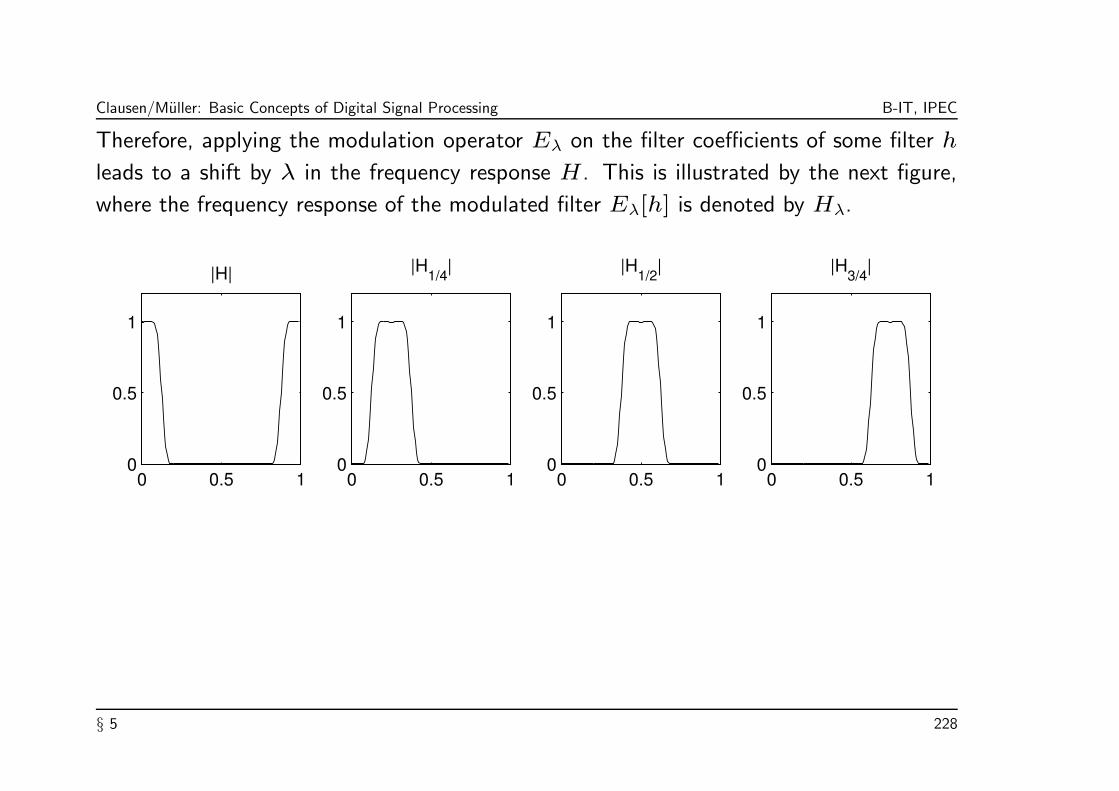
Clausen/Muller: Basic Concepts of Digital Signal Processing B-IT, IPEC
Therefore, applying the modulation operator Eλ on the filter coefficients of some filter h
leads to a shift by λ in the frequency response H. This is illustrated by the next figure,
where the frequency response of the modulated filter Eλ[h] is denoted by Hλ.
0 0.5 10
0.5
1
|H|
0 0.5 10
0.5
1
|H1/4
|
0 0.5 10
0.5
1
|H1/2
|
0 0.5 10
0.5
1
|H3/4
|
§ 5 228

Clausen/Muller: Basic Concepts of Digital Signal Processing B-IT, IPEC
The problem, however, is that Eλ[h] has in general complex filter coefficients even if h
has real coefficients. One possible trick is to consider the real part (or imaginary part) of
the modulated filter. For example, let
gλ := re(Eλ[h]),
then
gλ(n) = cos(2πλn)h(n) =1
2(e
2πiλn+ e
−2πiλn)h(n).
One also says that gλ arises from cosine-modulation from h.
§ 5 229

Clausen/Muller: Basic Concepts of Digital Signal Processing B-IT, IPEC
We now investigate which effect cosine-modulation has in the frequency domain. Let Gλ
denote the frequency response of gλ. Then
Gλ(ω) =∑
n∈Z
g(n)e−2πiωn
=∑
n∈Z
h(n) · 1
2(e
2πiλn − e−2πiλn
)e−2πiωn
=1
2
∑
n∈Z
h(n)e−2πi(ω−λ)n
+1
2
∑
n∈Z
h(n)e−2πi(ω+λ)n
=1
2(H(ω + λ) +H(ω − λ))
We give some examples to illustrate this effect. To distinguish the cut-off frequencies of
different filters, we write the filter as argument of the cut-off frequency.
§ 5 230

Clausen/Muller: Basic Concepts of Digital Signal Processing B-IT, IPEC
Example 5.2. Let h be an ideal lowpass filter with cut-off frequency ω0(h) ≤ 1/4 and
λ = 1/2. Then g1/2 is the ideal highpass with cut-off frequency ω0(g1/2) = 1/2−ω0(h).
0 10 20 30
−0.2
−0.1
0
0.1
0.2
0.3
h
0 0.25 0.5 0.75 10
0.2
0.4
0.6
0.8
1
|H|
0 10 20 30
−0.2
−0.1
0
0.1
0.2
0.3
g1/2
Time n0 0.25 0.5 0.75 1
0
0.2
0.4
0.6
0.8
1
|G1/2
|
Frequency ω
Note that in this case the cosine-modulation amounts to g1/2(n) = (−1)nh(n).
§ 5 231

Clausen/Muller: Basic Concepts of Digital Signal Processing B-IT, IPEC
The lowpass filter h and the highpass filter g1/2 have been applied to some chirp signal
x. Note that due to aliasing the frequency decreases at the end of the signal.
−1
−0.5
0
0.5
1
Chirp signal x
−1
−0.5
0
0.5
1
h*x
0 100 200 300 400 500 600 700 800 900 1000
−1
−0.5
0
0.5
1
g1/2
*x
Index n
§ 5 232

Clausen/Muller: Basic Concepts of Digital Signal Processing B-IT, IPEC
Example 5.3. Let h be an ideal lowpass filter with cut-off frequency ω0(h) ≤ 1/8
and λ = 1/4 Then g1/4 is (up to a factor 1/2) an ideal bandpass filter with
ω0(g1/4) = 1/4 − ω0(h) and ω1(g1/4) = 1/4 + ω0(h).
0 10 20 30
−0.2
−0.1
0
0.1
0.2
0.3
h
0 0.25 0.5 0.75 10
0.2
0.4
0.6
0.8
1
|H|
0 10 20 30
−0.2
−0.1
0
0.1
0.2
0.3
g1/4
Time n0 0.25 0.5 0.75 1
0
0.2
0.4
0.6
0.8
1
|G1/4
|
Frequency ω
§ 5 233

Clausen/Muller: Basic Concepts of Digital Signal Processing B-IT, IPEC
The bandpass filter g1/4 has been applied to the same chirp signal x as in the last
example.
−1
−0.5
0
0.5
1
Chirp signal x
0 100 200 300 400 500 600 700 800 900 1000
−1
−0.5
0
0.5
1
g1/4
*x
Index n
§ 5 234

Clausen/Muller: Basic Concepts of Digital Signal Processing B-IT, IPEC
Example 5.4. The following figure shows some highpass filter which let high frequencies
pass through, attenuates the frequencies in the middle and cuts off low frequencies.
0 10 20 30
−0.2
−0.1
0
0.1
0.2
0.3
h
0 0.25 0.5 0.75 10
0.2
0.4
0.6
0.8
1
|H|
0 10 20 30
−0.2
−0.1
0
0.1
0.2
0.3
g5/12
Time n0 0.25 0.5 0.75 1
0
0.2
0.4
0.6
0.8
1
|G5/12
|
Frequency ω
§ 5 235

Clausen/Muller: Basic Concepts of Digital Signal Processing B-IT, IPEC
Again we see the effect of the filter g5/12 on the chirp signal x.
−1
−0.5
0
0.5
1
Chirp signal x
0 100 200 300 400 500 600 700 800 900 1000
−1
−0.5
0
0.5
1
g5/12
*x
Index n
§ 5 236

Clausen/Muller: Basic Concepts of Digital Signal Processing B-IT, IPEC
Note 5.5. In case h ia a causal, linear-phase FIR filter of length M a slight modification
of above cosine-moulation
gλ(n) = cos
(2πλ
(n− M − 1
2
))h(n)
again yields a causal, linear-phase FIR filter gλ of the same length.
§ 5 237

Clausen/Muller: Basic Concepts of Digital Signal Processing B-IT, IPEC
Modulation of filters play an important role in the design of filter banks. Here one starts
with a single “prototype” filter and generates a whole set of other filters by suitable
modulations of this prototype filter. Ideally
• each of these filters covers a band in the spectral domain,
• the bands of different filters do not overlap, and
• the union of the bands cover the whole spectral domain.
In view of the perfect reconstruction condition of a filter bank and an efficient simultaneous
evaluation of all filters, the cosine-modulation has to be carefully designed (amounting in
choosing suitable phases in the cosines).
For further details on this topic we refer to [Burrus/Gopinath/Guo].
§ 5 238

Clausen/Muller: Basic Concepts of Digital Signal Processing B-IT, IPEC
Chapter 6: Windowed Fourier Transform (WFT)
The Fourier transform f of a signal f ∈ L2(R) describes the frequency content of the
signal. The time dependent f is transformed into a frequency dependent signal
f(ω) :=
∫ ∞
−∞f(t)e
−2πiωtdt.
Intuitively, the signal f is analyzed by means of the exponential functions
R → C, t 7→ e2πiωt
of different frequencies ω ∈ R. These analysis functions are periodic and not localized
w.r.t. time. In this sense they are well suited to analyze the in general non-periodic signal
f ∈ L2(R).
§ 6 239

Clausen/Muller: Basic Concepts of Digital Signal Processing B-IT, IPEC
Summarizing, the Fourier transform can be interpreted as follows:
• The Fourier transform hides the information about time (in the phase). It tells which
“notes” (frequencies) are played, but it does not tell when these notes are played.
• Sudden changes und local variations of the signal as well as the beginning and the end
of events cannot be detected by the Fourier transform.
• The frequency information is always averaged over the entire time interval.
• Local phenomena of the signal become global phenomena in the Fourier transform.
• Contrary, small changes in the phase of the Fourier transform can have considerable
effects in the time domain.
§ 6 240

Clausen/Muller: Basic Concepts of Digital Signal Processing B-IT, IPEC
To remedy the drawbacks of the Fourier transform Dennis Gabor introduced in the
year 1946 the modified Fourier transform, now known as windowed Fourier transform or
simply WFT. This transform is a compromise between a time- and a frequency-based
representation of the signal. The WFT does not only tell which frequencies are “contained”
in the signal but also at which points of times or, to be more precise, in which time
intervals these frequencies appear.
§ 6 241

Clausen/Muller: Basic Concepts of Digital Signal Processing B-IT, IPEC
6.1 Defintion of the WFT
For a given signal f ∈ L2(R) we want to find a transform, f(ω, t) which exhibits the
frequency distribution at the point t. The basic idea for the design of such a transform
comes from the way the human auditory system performs a realtime analysis of audio
signals:
• For the analysis only a small section of the signal which lies directly behind the present
point of time is used for the analysis.
• The further the points of time in this section lie in the past, the less they will be
considered.
• Similar, the audio signal at “current” points of time is not yet percieved very well and
therefore also less considered.
§ 6 242

Clausen/Muller: Basic Concepts of Digital Signal Processing B-IT, IPEC
Mathematically, this weighting of the signal is modeled by multiplying the signal with a
window function. The window function can be thought of as a bell-shaped function which
localizes around t = 0.
If f ∈ L2(R) is a signal and g : R → C is a window function, then the function fg,tlocalized at point t is defined by
fg,t(u) := f(t, u) := g(u− t)f(u).
If g is known from the context, then one also writes just ft instead of fg,t. For the
moment, we just assume g ∈ L2(R) and ||g||2 6= 0.
§ 6 243

Clausen/Muller: Basic Concepts of Digital Signal Processing B-IT, IPEC
Definition 6.1. Let g ∈ L2(R), ||g||2 6= 0, be a window function. Then for a signal
f ∈ L2(R) the transform
f(ω, t) :=
∫ ∞
−∞ft(u)e
−2πiωudu =
∫ ∞
−∞g(u− t)f(u)e
−2πiωudu
is called the windowed Fourier transform (WFT) of f (with respect to g).
If we define the function gω,t : R → C by
gω,t(u) := e2πiωu
g(u− t), u ∈ R,
then ||gω,t|| = ||g||, gω,t ∈ L2(R), and the WFT of f can be written as
f(ω, t) = 〈f |gω,t〉.
§ 6 244

Clausen/Muller: Basic Concepts of Digital Signal Processing B-IT, IPEC
Intuitively, the WFT can be thought of as follows:
• The function gω,t represents a “musical note” of frequency ω which oscillates within
the translated window given by u 7→ |g(u− t)|.• The inner product 〈f |gω,t〉 measures the correlation between the signal f and the
musical note gω,t. If f and gω,t have a similar course in time within the window, the
inner product 〈f |gω,t〉 has a large absolute value and vice versa.
• The signal
u 7→ 〈f |gω,t〉gω,t(u)
can be considered as the “projection” of the signal f in direction of the musical note
gω,t.
§ 6 245

Clausen/Muller: Basic Concepts of Digital Signal Processing B-IT, IPEC
6.2 Examples
6.2.1 Window Functions
As an example, Figure 12 shows three different window functions with their respective
spectral energy density.
Using the box-window g, the signal f is preserved on the support supp(g) = [−0.5, 0.5]
and is set to zero outside this support. The box-window has a major drawbacks. The
localized functions fg,t defined by
fg,t(u) := f(t, u) := g(u− t)f(u)
have in general considerable discontinuities at the cuts which cause artefacts and
interferencies seen in the frequency domain.
We remind that short-time events and abrupt changes in the signal lead to high-frequency
phenomena in the Fourier domain.
§ 6 246

Clausen/Muller: Basic Concepts of Digital Signal Processing B-IT, IPEC
The Hanning window g defined by
g(u) :=
1 + cos(πu) falls −1 ≤ u ≤ 1
0 sonst
was already introduced in Example 2.26. The Hanning window has also compact support,
however, it abates smoothly when reaching the support boundaries. Therefore, the above
mentioned artefacts in the Fourier transform of the windowed signal are softened. This is
also illustrated by comparing Figure 13 with Figure 14.
§ 6 247
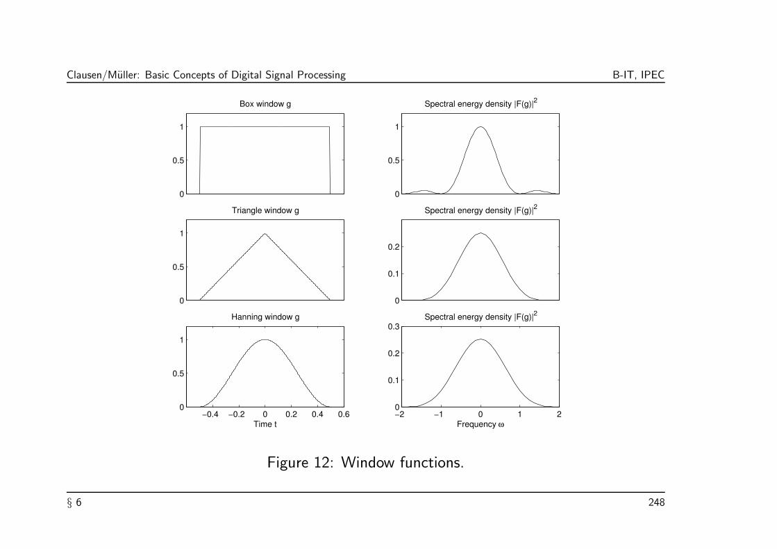
Clausen/Muller: Basic Concepts of Digital Signal Processing B-IT, IPEC
0
0.5
1
Box window g
0
0.5
1
Spectral energy density |F(g)|2
0
0.5
1
Triangle window g
0
0.1
0.2
Spectral energy density |F(g)|2
−0.4 −0.2 0 0.2 0.4 0.60
0.5
1
Time t
Hanning window g
−2 −1 0 1 20
0.1
0.2
0.3
Frequency ω
Spectral energy density |F(g)|2
Figure 12: Window functions.
§ 6 248
Clausen/Muller: Basic Concepts of Digital Signal Processing B-IT, IPEC
There are many other window functions used in the WFT. For further information we refer
to the MatLab handbook.
Finally, we want to mention, that the window function does not necessarily have to have a
compact support. One example is the Gauss window shown in Example 2.15. The choice
of the “right” window function constitutes often a difficult problem and depends on the
respective application.
§ 6 249

Clausen/Muller: Basic Concepts of Digital Signal Processing B-IT, IPEC
6.2.2 WFT of a Chirp Signal
Figure 13 shows the time-frequency representation of the chirp signal f defined by
f(t) = sin(400πt2), t ∈ R
using the WFT w.r.t. the Hanning window. The values
|f(ω, t)| = |〈f |gω,t〉|
at (t, ω) is represented by different gray levels, which are lighter for small values |f(ω, t)|and darker for large values |f(ω, t)|.
§ 6 250

Clausen/Muller: Basic Concepts of Digital Signal Processing B-IT, IPEC
0 0.1 0.2 0.3 0.4 0.5 0.6 0.7 0.8 0.9 1−1
01
Chirp function f(t)=sin(400π t2) and WFT with Hanning window of length 0.05
Time
Freq
uenc
y
0 0.1 0.2 0.3 0.4 0.5 0.6 0.7 0.8 0.90
100
200
300
400
500
600
700
800
900
1000
Figure 13: WFT with Hanning window.
§ 6 251

Clausen/Muller: Basic Concepts of Digital Signal Processing B-IT, IPEC
We want to make some comments on Figure 13.
(1) As one might expect from a time-frequency representation of a chirp signal, the large
values |f(ω, t)| lie on the diagonal ω = 800 · t (which corresponds up to a factor 2π
to the derivative of the phase).
(2) Furthermore, the figure shows some diagonals below and above the main diagonal
which reflect small parasitic frequency arising from the destructive intereference
mentioned in Example 2.12.
§ 6 252
Clausen/Muller: Basic Concepts of Digital Signal Processing B-IT, IPEC
(3) The dark areas in the upper left and lower right corner in the time-frequency
representation are not based on the properties of f or g but are caused by
approximation errors. In the actual computations of the WFT by computer, the
integrals 〈f |gω,t〉 have been approximated by Riemann sums. The more the function
f · gω,t oscillates, the worse get the approximations of the integral 〈f |gω,t〉 by these
sums. Therefore, we have large approximation errors in the mentioned areas: in the
upper area left since gω,t has large oscillations for large ω and in the lower right area
since f has large oscillations for large t.
§ 6 253

Clausen/Muller: Basic Concepts of Digital Signal Processing B-IT, IPEC
Figure 14 shows the time-frequency representation where for the WFT the box window
was used instead of the Hanning window.
The abrupt cuts at the support boundaries introduced by box window cause interferences
all over the spectrum. Figure 14 shows that the dark areas and hence the large values of
|f(ω, t)| are spread all over the time-frequency domain. The large values of |f(ω, t)|are not as well concentrated around the diagonal ω = 800 · t as it was in case of the
Hanning window. Hence, using the box functions, leads to an “inferior” time-frequency
respresentation of the chirp signal.
§ 6 254
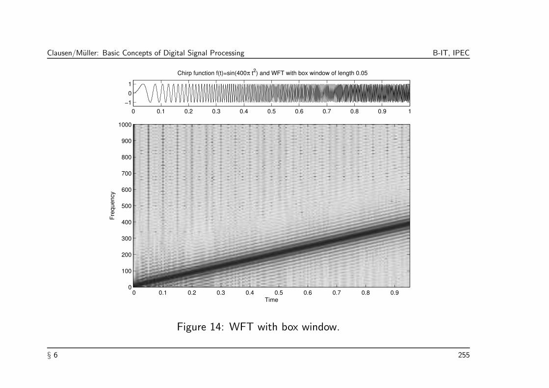
Clausen/Muller: Basic Concepts of Digital Signal Processing B-IT, IPEC
0 0.1 0.2 0.3 0.4 0.5 0.6 0.7 0.8 0.9 1−1
01
Chirp function f(t)=sin(400π t2) and WFT with box window of length 0.05
Time
Freq
uenc
y
0 0.1 0.2 0.3 0.4 0.5 0.6 0.7 0.8 0.90
100
200
300
400
500
600
700
800
900
1000
Figure 14: WFT with box window.
§ 6 255

Clausen/Muller: Basic Concepts of Digital Signal Processing B-IT, IPEC
6.2.3 WFT in Dependence of the Window Size
In this example we consider the signal f defined on [0, 1] by
f(t) = sin(800πt) + sin(900πt) + c[δ(t− 0.45) + δ(t− 0.5)]
with a small constant c ∈ R and zero on R \ [0, 1]. f is the superposition of two pure
sines of frequency ω1 = 400 and ω2 = 450, respectively, and two additional impulses at
t1 = 0.45 and t2 = 0.5.
The Figures 15 and 16 show the time-frequency representation of f using a WFT w.r.t.
a Hanning window — however, with different window sizes. In the first case the window
size was chosen to be 0.02 and in the second case to be 0.1.
§ 6 256

Clausen/Muller: Basic Concepts of Digital Signal Processing B-IT, IPEC
0 0.1 0.2 0.3 0.4 0.5 0.6 0.7 0.8 0.9 1−2
02468
f(t)=sin(800π t)+sin(900π t), peaks at x=0.45, x=0.5, and WFT with Hanning window of length 0.02
Time t
Freq
uenc
y ω
0 0.1 0.2 0.3 0.4 0.5 0.6 0.7 0.8 0.90
100
200
300
400
500
600
700
800
900
1000
Figure 15: WFT using a small window size.
§ 6 257

Clausen/Muller: Basic Concepts of Digital Signal Processing B-IT, IPEC
0 0.1 0.2 0.3 0.4 0.5 0.6 0.7 0.8 0.9 1−2
02468
f(t)=sin(800π t)+sin(900π t), peaks at x=0.45, x=0.5, and WFT with Hanning window of length 0.1
Time t
Freq
uenc
y ω
0 0.1 0.2 0.3 0.4 0.5 0.6 0.7 0.8 0.90
100
200
300
400
500
600
700
800
900
1000
Figure 16: WFT using a large window size.
§ 6 258

Clausen/Muller: Basic Concepts of Digital Signal Processing B-IT, IPEC
Comparing the two figures one can make the following observations:
(1) For the larger window size of 0.1 (Figure 16) one has a good resolution in the
time-frequency representation of the two pure sine oscillations. However, the tow peaks
at t1 and t2 are poorly separated.
(2) Using the smaller window size of 0.02 (Figure 15) one has a good resolution of the
two peaks but the two frequencies ω1 and ω2 of the sines are “smeared”.
§ 6 259

Clausen/Muller: Basic Concepts of Digital Signal Processing B-IT, IPEC
This phenomena are based on a general principle:
(1) Increasing the window size of the window function g leads to a WFT (w.r.t. g) which
“averages” the frequencies of the signal f over a greater time segment. Therefore,
time information is lost. (In the limit case of an “infinite window size” one derives at
the usual Fourier transform which averages the frequencies over all of R.)
(2) Decreasing the window size leads to a better time resolution of the corresponding
WFT. However, in this case the lower frequencies of the signal f cannot any longer
be seized by the WFT since they are dominated by the window size. This leads to
the above mentions smearing effects for low-frequency phenomena. (In the limit case,
g is an impulse and the WFT gives back the signal f : perfect time information, no
frequency information.)
§ 6 260

Clausen/Muller: Basic Concepts of Digital Signal Processing B-IT, IPEC
6.3 Time-Frequency Localization of the WFT
We want to look at the coefficients f(ω, t) from two different perspectives: a time- and
a frequency-based one. Let f ∈ L2(R) be a signal and g ∈ L2(R), ||g||2 6= 0 be a
window. Then, by Parseval’s Identity,
f(ω, t) = 〈f |gω,t〉 = 〈f |gω,t〉.
In other words, one has the following two representations for f(ω, t):
(1) f(ω, t) = 〈f |gω,t〉 =∫∞−∞ f(u)g(u− t)e−2πiωudu
(2) f(ω, t) = 〈f |gω,t〉 = e−2πiωt∫∞−∞ f(v)
¯g(v − ω)e2πivtdv
§ 6 261

Clausen/Muller: Basic Concepts of Digital Signal Processing B-IT, IPEC
These two representations allow the following interpretations:
(1) Let t0 be a point of time. The signal f is windowed by u 7→ g(u − t0) und
Fourier transformed. Then |f(ω, t0)| tells which frequencies “appear” in f in the
neighborhood of t0.
(2) Let ω0 be a frequency. The Fourier transform f is windowed by v 7→ ¯g(v−ω0) and
inverse Fourier transformed. Then |f(ω0, t)| tells in which points of time the signal f
contains the frequencies in a neighborhood of ω0.
§ 6 262
Clausen/Muller: Basic Concepts of Digital Signal Processing B-IT, IPEC
The neighborhood of t0 in (1) is determined by the localization property of the window
function g. Similarly, the neighborhood of ω0 in (2) is determined by the localization
property of the Fourier transform g of the window function.
If one wants to have in the time-frequency representation of a signal f a good resolution
in time as well as in frequency, the window function g should have a good localization in
time (property on g) as well as in frequency (property on g).
However, the Heisenberg uncertainty principle says that this simultaneous localization of g
is only possible up to a certain degree.
§ 6 263
Clausen/Muller: Basic Concepts of Digital Signal Processing B-IT, IPEC
6.3.1 Heisenberg Uncertainty Principle
Formally, the localization property of a window function g ∈ L2(R) with ||g|| = 1 can be
defined by using the notions of the center t0(g) and the width T (g) of g, where
t0 = t0(g) :=
∫ ∞
−∞t|g(t)|2dt and T (g) :=
(∫ ∞
−∞(t− t0)
2|g(t)|2dt)1
2
.
Analogously, one defines the center ω0(g) and the width Ω(g) for the Fourier transform
g by
ω0 = ω0(g) :=
∫ ∞
−∞ω|g(ω)|2dω and Ω(g) :=
(∫ ∞
−∞(ω − ω0)
2|g(ω)|2dω)1
2
.
§ 6 264

Clausen/Muller: Basic Concepts of Digital Signal Processing B-IT, IPEC
If the window function g is known from the context, we also simply write t0, T , ω0
and Ω without the arguement g. Mathematically, the center t0 is the expectation and
T the standard deviation of the random variable t 7→ |g(t)|2. In general, the center
and width for arbitrary functions g ∈ L2(R) are not defined. (These values could be
infinite.) In case both values are finite, we say that g localizes at t0 with window width
T . Analogously, we say that g localizes at frequency ω0 with bandwidth Ω.
As motivated before, we are interested in a window function which localizes in time as well
as in frequency. The Heisenberg uncertainty principle says that this is not possible with
arbitrary precision.
§ 6 265
Clausen/Muller: Basic Concepts of Digital Signal Processing B-IT, IPEC
Theorem 6.2. [Heisenberg Uncertainty Principle] Let g ∈ L2(R) with ||g|| = 1,
center t0(g) and width T (g). Furthermore, let ω0(g) and Ω(g) be the center and
width of g, respectively. Then
T (g) · Ω(g) ≥ 1
4π.
Squaring both sides yields
(∫ ∞
−∞(t− t0)
2|g(t)|2dt)(∫ ∞
−∞(ω − ω0)
2|g(ω)|2dω)
≥ 1
16π2.
§ 6 266

Clausen/Muller: Basic Concepts of Digital Signal Processing B-IT, IPEC
Proof:
We prove this assertion only for g ∈ L2(R), which are continuously differentiable such
that the derivative g′ is also in L2(R). One can show that such functions form a dense
subset of L2(R). For arbitrary functions in L2(R) the assertion follows then by some
approximation argument. We refer to the literature for such a proof.
We simplify the problem stepwise.
(1) In case T (g) or Ω(g) is infinite, the assertion of the theorem becomes obvious.
Therefore, we now may restrict ourselves to functions g ∈ L2(R) for which both of
these values are finite.
§ 6 267

Clausen/Muller: Basic Concepts of Digital Signal Processing B-IT, IPEC
(2) For some g ∈ L2(R) define h ∈ L2(R) by
h(t) := e−2πiω0tg(t+ t0).
By Theorem 2.9,
h(ω) = e2πit0(ω+ω0)
g(ω + ω0).
From this it is easy to see that h is centered, i.e., t0(h) = 0 and ω0(h) = 0, and
(∫ ∞
−∞t2|h(t)|2dt
)(∫ ∞
−∞ω
2|h(ω)|2dω)
=
(∫ ∞
−∞(t− t0)
2|g(t)|2dt)(∫ ∞
−∞(ω − ω0)
2|g(ω)|2dω).
In other words, it suffices to show the Heisenberg uncertainty principle for centered
functions.
§ 6 268

Clausen/Muller: Basic Concepts of Digital Signal Processing B-IT, IPEC
In the following let g ∈ L2(R) with ||g|| = 1, t0(g) = 0, and ω0(g) = 0. Furthermore,
let T (g) and Ω(g) be finite, g differentiable, and g′ ∈ L2(R). Then using
ωg(ω) = 12πig
′(ω) and Parseval’s equation ||g′|| = ||g′||, we obtain
T (g)2 · Ω(g)
2=
(∫ ∞
−∞t2|g(t)|2dt
)(∫ ∞
−∞ω
2|g(ω)|2dω)
=1
4π2
(∫ ∞
−∞t2|g(t)|2dt
)(∫ ∞
−∞|g′(t)|2dt
)
§ 6 269

Clausen/Muller: Basic Concepts of Digital Signal Processing B-IT, IPEC
From the Cauchy-Schwarz inequality ||f1||2||f2||2 ≥ |〈f1|f2〉|2 with f1(t) = |tg(t)| and
f2(t) = |g′(t)| follows
1
4π2
(∫ ∞
−∞t2|g(t)|2dt
)(∫ ∞
−∞|g′(t)|2dt
)
≥ 1
4π2
(∫ ∞
−∞|tg(t)g′(t)|dt
)2
≥ . . .
For arbitrary complex numbers a, b ∈ C holds |ab| = |ab| ≥ Re(ab) = 12(ab + ab).
Using this for a = tg(t) and b = g′(t) one gets
. . . ≥ 1
4π2
(1
2
∫ ∞
−∞(tg(t)g′(t) + tg(t)g
′(t))dt
)2
§ 6 270
Clausen/Muller: Basic Concepts of Digital Signal Processing B-IT, IPEC
Using ddt|g(t)|2 = g(t)g′(t) + g′(t)g(t),
∫∞−∞ t|g(t)|
2dt = t0(g) = 0 and hence
limt→∞ t|g(t)|2 = 0, it follows by partial integration that
1
4π2
(1
2
∫ ∞
−∞(tg(t)g′(t) + tg(t)g
′(t))dt
)2
≥ 1
16π2
(−∫ ∞
−∞|g(t)|2dt
)2
=1
16π2||g||4.
Since ||g|| = 1, the assertion follows.
§ 6 271

Clausen/Muller: Basic Concepts of Digital Signal Processing B-IT, IPEC
Note 6.3. The boundary in the Heisenberg uncertainty principle is sharp. Indeed, one can
show that for the Gauss function (see also Example 2.15) gω0,t0defined by
gω0,t0(t) := π
−14
1√2πe−2πiω0te
−π(t−t0)2
holds t0(gω0,t0) = t0, ω0(gω0,t0
) = ω0 and
T (gω0,t0) · Ω(gω0,t0
) =1
4π.
Furthermore, it holds that this function is the only function with minimal uncertainty at
(t0, ω0).
§ 6 272

Clausen/Muller: Basic Concepts of Digital Signal Processing B-IT, IPEC
Note 6.4. We close this subsection with some more intuitive notes on the principle which
are partly taken from [Hubbard].
• The Heisenberg uncertainty principle has its origin in quantum physics. Intuitively it
says that an elementary particle does not simultaneously have a precise position and a
precise momentum. In our case this principle says that a signal does not simultaneously
have a precise location in time and a precise frequency.
• A very brief signal, well localized in time, necessarily has a Fourier transform that is
spread out: a broad range of frequencies. Conversely, a signal with a very narrow
range of frequencies is necessarily spread in time; it’s not possible to convince just a
few sines and cosines to cancel out so that the vlaues of the signal is small outside a
narrow time interval.
• The time parameter t in f(ω, t) of the WFT is not sharp but represents a time
interval, which depends on the window width of g. Similar holds for the frequency
parameter ω. The choice of the window function g determines the “resolution
proportion” between time and frequency.
§ 6 273
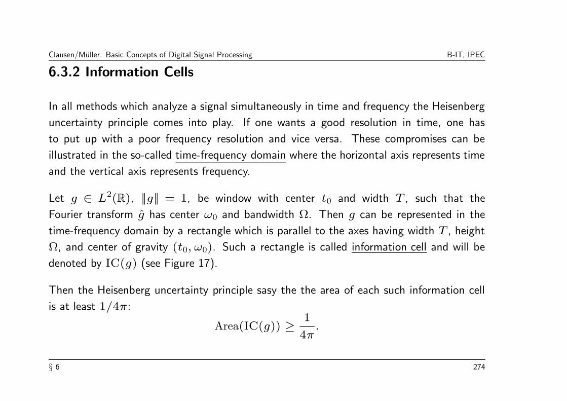
Clausen/Muller: Basic Concepts of Digital Signal Processing B-IT, IPEC
6.3.2 Information Cells
In all methods which analyze a signal simultaneously in time and frequency the Heisenberg
uncertainty principle comes into play. If one wants a good resolution in time, one has
to put up with a poor frequency resolution and vice versa. These compromises can be
illustrated in the so-called time-frequency domain where the horizontal axis represents time
and the vertical axis represents frequency.
Let g ∈ L2(R), ||g|| = 1, be window with center t0 and width T , such that the
Fourier transform g has center ω0 and bandwidth Ω. Then g can be represented in the
time-frequency domain by a rectangle which is parallel to the axes having width T , height
Ω, and center of gravity (t0, ω0). Such a rectangle is called information cell and will be
denoted by IC(g) (see Figure 17).
Then the Heisenberg uncertainty principle sasy the the area of each such information cell
is at least 1/4π:
Area(IC(g)) ≥ 1
4π.
§ 6 274

Clausen/Muller: Basic Concepts of Digital Signal Processing B-IT, IPEC
ω
ω+ω
t t+t
0
0
0 0
T
T
Ω
Ω
IZ(g)
IZ(g )ω, t
Figure 17: Information cells for g and gω,t.
§ 6 275

Clausen/Muller: Basic Concepts of Digital Signal Processing B-IT, IPEC
One easily computes that the information cell of the “musical note”
gω,t : R → C, gω,t(u) := e2πiωu
g(u− t)
for a window g as above has also width T and height Ω with center of gravity
(t0 + t, ω0 + ω). The WFT
f(ω, t) = 〈f |gω,t〉of a signal f ∈ L2(R) w.r.t. the window function g gives an analysis of f in the area
of the information cell of gω,t. In the time-frequency domain the WFT is depicted by
representing the value 〈f |gω,t〉 over the information cell of gω,t with a suitable grey color.
If one considers the WFT only on a discrete grid of points in the time-frequency domain,
one gets a tiling of the time-frequency domain by (possibly overlapping) congruent
information cells, where the grey levels reflect the time-frequency information of the signal
f .
§ 6 276

Clausen/Muller: Basic Concepts of Digital Signal Processing B-IT, IPEC
6.3.3 Reconstruction of the Signal from its WFT
Let f ∈ L2(R) be a signal with WFT f(ω, t) w.r.t the window function g ∈ L2(R),
||g|| 6= 0. As explained in Section 1, the value f(ω, t) expresses in which intensity the
note gω,t is “contained” in the signal f . Therfore, intuitively, one should be able to
reconstruct the signal f as superposition of the notes gω,t weighted by 〈f |gω,t〉:
f(u) ∼∫
R
∫
R
〈f |gω,t〉gω,t(u)dωdt.
We will now show that this is indeed correct up to a normalizing factor.
§ 6 277
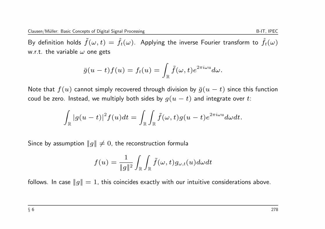
Clausen/Muller: Basic Concepts of Digital Signal Processing B-IT, IPEC
By definition holds f(ω, t) = ft(ω). Applying the inverse Fourier transform to ft(ω)
w.r.t. the variable ω one gets
g(u− t)f(u) = ft(u) =
∫
R
f(ω, t)e2πiωu
dω.
Note that f(u) cannot simply recovered through division by g(u− t) since this function
coud be zero. Instead, we multiply both sides by g(u− t) and integrate over t:
∫
R
|g(u− t)|2f(u)dt =
∫
R
∫
R
f(ω, t)g(u− t)e2πiωu
dωdt.
Since by assumption ||g|| 6= 0, the reconstruction formula
f(u) =1
||g||2∫
R
∫
R
f(ω, t)gω,t(u)dωdt
follows. In case ||g|| = 1, this coincides exactly with our intuitive considerations above.
§ 6 278
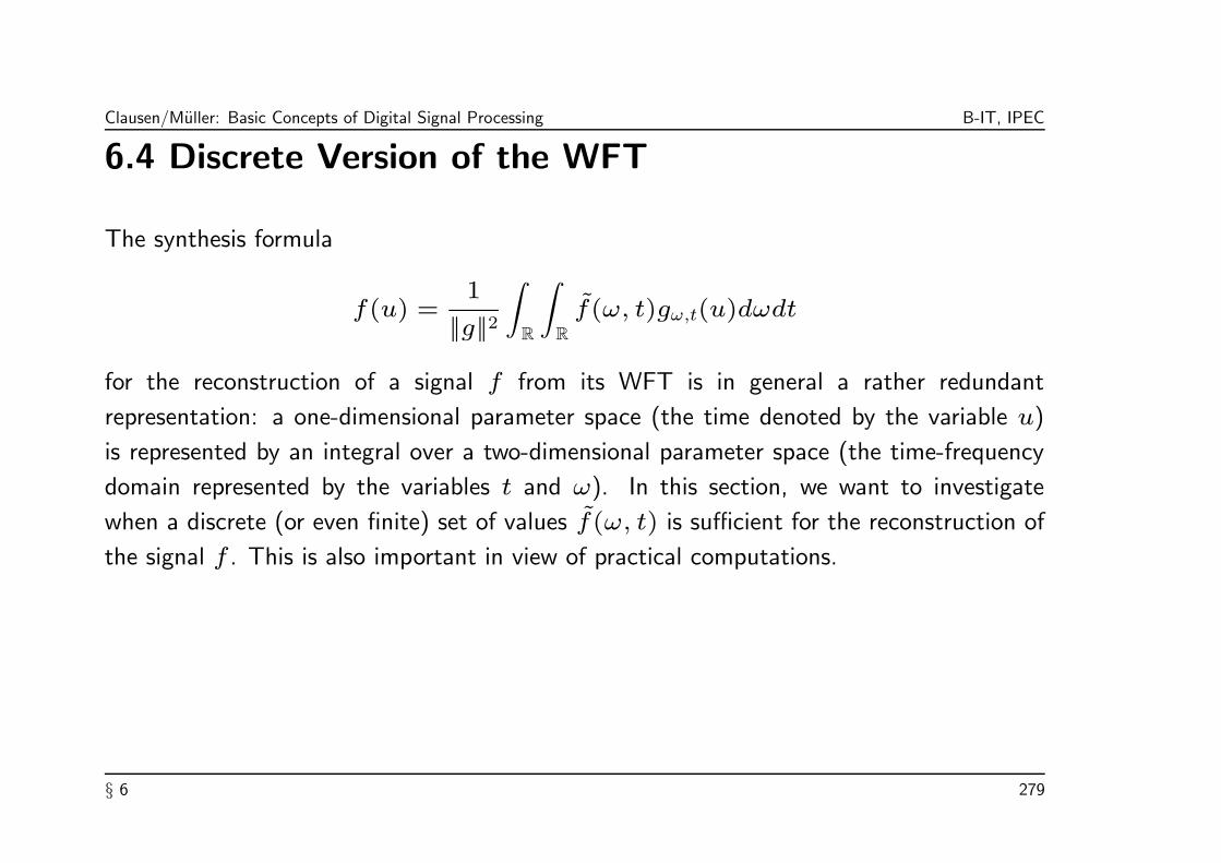
Clausen/Muller: Basic Concepts of Digital Signal Processing B-IT, IPEC
6.4 Discrete Version of the WFT
The synthesis formula
f(u) =1
||g||2∫
R
∫
R
f(ω, t)gω,t(u)dωdt
for the reconstruction of a signal f from its WFT is in general a rather redundant
representation: a one-dimensional parameter space (the time denoted by the variable u)
is represented by an integral over a two-dimensional parameter space (the time-frequency
domain represented by the variables t and ω). In this section, we want to investigate
when a discrete (or even finite) set of values f(ω, t) is sufficient for the reconstruction of
the signal f . This is also important in view of practical computations.
§ 6 279

Clausen/Muller: Basic Concepts of Digital Signal Processing B-IT, IPEC
We assume in this section that the window function g has compact support contained in
the interval [a, b] ⊂ R. Then the localized signal ft(u) := g(u − t)f(u) has support
in [a+ t, b+ t] and can therefore on this interval be represented by the Fourier series
ft(u) =∑
m∈Z
〈ft|1√TeT,m〉
1√TeT,m(u), (10)
where T := b− a and the functions eT,m are defined by
eT,m(u) := e2πium/T
, m ∈ Z.
Note that ( 1√NeT,m)m∈Z form an ONB of the Hilbert space L2([a + t, b + t]) with
inner product 〈f |g〉 =∫ b+ta+t
f(u)g(u)du. We emphasize that this equality only hold for
u ∈ [a+ t, b+ t].
§ 6 280

Clausen/Muller: Basic Concepts of Digital Signal Processing B-IT, IPEC
The value ν := 1b−a = 1
T is called frequency step width and represents the distance
between two neighboring frequencies to be analyzed. Then
〈ft|eT,m〉 =
∫ b+t
a+t
g(u− t)f(u)e−2πimνu
du
=
∫ ∞
−∞g(u− t)f(u)e
−2πimνudu
= f(mν, t).
Multiplying both sides of the Fourier series representation (10) by g(u− t) one gets
|g(u− t)|2f(u) = ν∑
m∈Z
g(u− t)f(mν, t)e2πimνu
.
§ 6 281

Clausen/Muller: Basic Concepts of Digital Signal Processing B-IT, IPEC
The goal is to isolate f(u) on the left hand side. To this means we define the function
Hτ(u) := τ∑
n∈Z
|g(u− nτ)|2
w.r.t. the time step width τ > 0. Hτ is well-defined since the support of g is assumed
to be compact. Furthermore, if g is Riemann integrable, Hτ defines a Riemann sum for
||g||2 and therefore
Hτ(u) → ||g||2 for τ → 0.
Summation over n with time step width τ results in
Hτ(u)f(u) = τν∑
n∈Z
∑
m∈Z
g(u− nτ)f(mν, nτ)e2πimνu
.
§ 6 282

Clausen/Muller: Basic Concepts of Digital Signal Processing B-IT, IPEC
We want to divide by Hτ which is only possible if Hτ(u) 6= 0 for almost all u. Let
Aτ := infu∈R
Hτ(u) and Bτ := supu∈R
Hτ(u).
Then one can show that for “nice” window functions g and for sufficiently small τ and all
u ∈ R holds
0 < Aτ ≤ Hτ(u) ≤ Bτ < ∞.
In this case we obtain a discrete WFT-reconstruction
f(u) = τν∑
n∈Z
∑
m∈Z
g(u− nτ)
Hτ(u)f(mν, nτ)e
2πimνu. (11)
The finiteness of Bτ assures the numerical stability of the summation.
§ 6 283

Clausen/Muller: Basic Concepts of Digital Signal Processing B-IT, IPEC
Note 6.5. For Aτ > 0 to be satisfied one needs 0 < τ ≤ b − a, since otherwise
Hτ(u) = 0 for b < u < a+ τ . With 0 < τ ≤ b− a and by definiton of ν holds
0 < τ · ν ≤ 1.
Then the sample density defined by
ρ(ν, τ) :=1
ν · τ =b− a
τ
is a measure for the redundancy of the representation (11) of f . For example, if
b − a = 1024 and τ = 256, then the sample density is 4, which is in real-time
applications a common value. The extreme case τ · ν = 1 contains no redundancy and,
as it turns out, is in practical computations numerically not stable.
§ 6 284

Clausen/Muller: Basic Concepts of Digital Signal Processing B-IT, IPEC
6.5 Drawback of the WFT
Even though the introduction of window functions leads to localization in time as well as
in frequency the analysis of a signal by the WFT has several drawbacks which we discuss
next.
The window function g introduces a kind of scaling in the time-frequency domain. In
other words, for a given g the width T and the height Ω of the corresponding information
cell IC(g) is determined once and for all. The signal f is analyzed by the notes gω,t on
the translated information cell IC(gω,t) = IC(g) + (t, ω).
As we explain next, the WFT is not efficient when the signal f contains phenomena which
are either of short duration or of long duration as compared to T .
§ 6 285

Clausen/Muller: Basic Concepts of Digital Signal Processing B-IT, IPEC
(1) Suppose the signal f contains a local oscillation or a peak of width ∆u T at
u = u0. Such a peak is in the WFT-synthesis represented as a superposition of notes
gω,t each of it having length T . This is only possible, if many of the notes gω,t with
t ≈ u0 of many different frequencies are used, due to the principle of constructive and
destructive interference. Therefore, f(ω, u0) is spread out in frequency at point of
time u0.
(2) We now suppose that f contains some large, global variations with ∆u T such
as a low-frequency sine oscillation. In this case many of the low-frequency notes gω,tare needed to synthesize f over ∆u. Therefore, f(ω, t) is spread out in time.
§ 6 286

Clausen/Muller: Basic Concepts of Digital Signal Processing B-IT, IPEC
The following principles
Principle 1: Properties of f , which are much shorter than T , are synthesized in the
frequency domain.
Principle 2: Properties of f , which are much longer than T , are synthesized in the time
domain.
In both cases many of the notes gω,t are needed to synthesize phenomena of the signal
f which are relatively simple in nature such as a peak or a low-frequency oscillation. In
other words, the WFT is not capable to capture such features in few, but large coefficients
f(ω, t) and is therefore not efficient.
In the following chapter we introduce the time-frequency analysis based on wavelets which
overcome some of the drawbacks of the WFT.
§ 6 287

Clausen/Muller: Basic Concepts of Digital Signal Processing B-IT, IPEC
Chapter 7: Continuous Wavelet Transform(CWT)
Just like the WFT, the wavelet transform also gives a time-frequency representation of a
signal. Analogously to the WFT, the continuous wavelet transform (CWT) of a signal
f ∈ L2(R) is defined by
f(s, t) := |s|−12
∫ ∞
−∞f(u)ψ
(u− t
s
)du,
where ψ ∈ L2(R) is a suitable function called mother wavelet.
§ 7 288
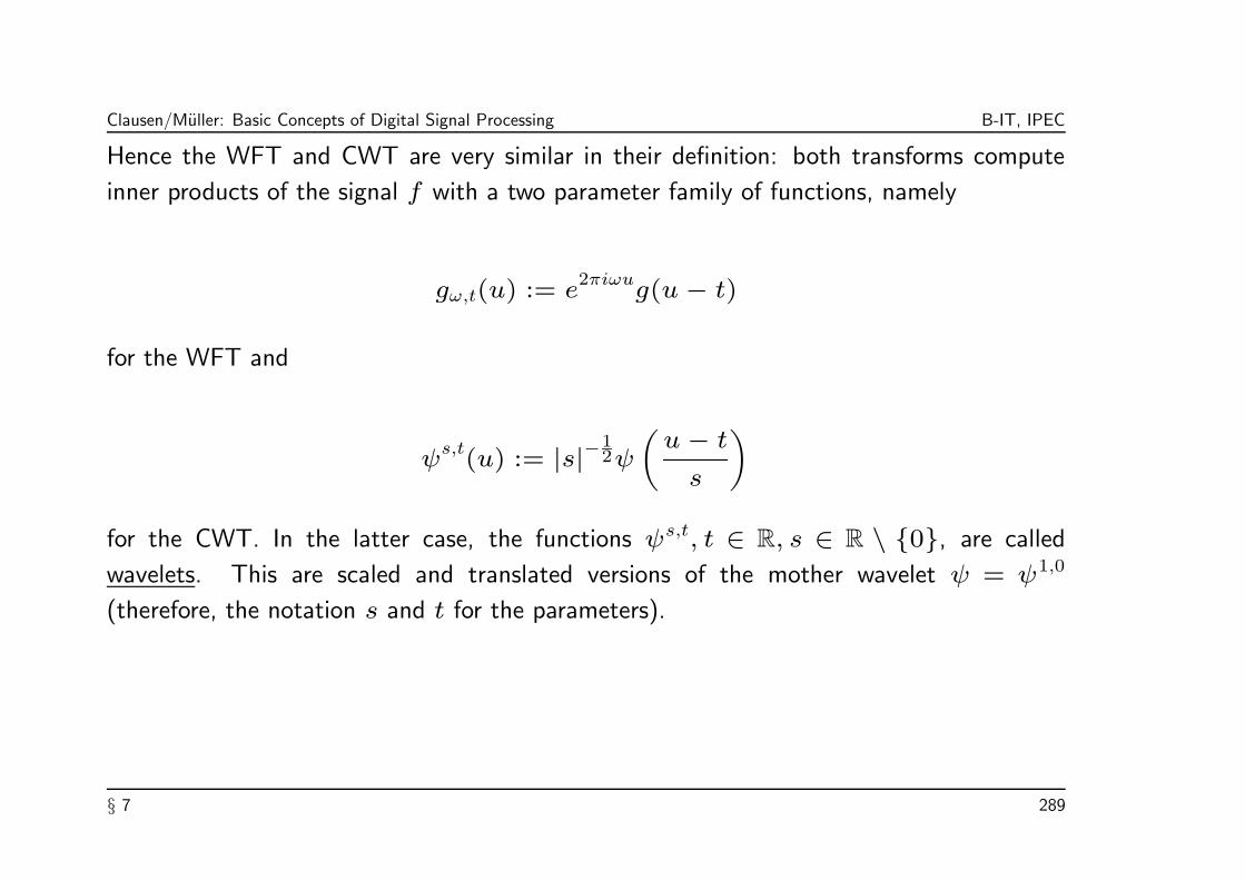
Clausen/Muller: Basic Concepts of Digital Signal Processing B-IT, IPEC
Hence the WFT and CWT are very similar in their definition: both transforms compute
inner products of the signal f with a two parameter family of functions, namely
gω,t(u) := e2πiωu
g(u− t)
for the WFT and
ψs,t
(u) := |s|−12ψ
(u− t
s
)
for the CWT. In the latter case, the functions ψs,t, t ∈ R, s ∈ R \ 0, are called
wavelets. This are scaled and translated versions of the mother wavelet ψ = ψ1,0
(therefore, the notation s and t for the parameters).
§ 7 289

Clausen/Muller: Basic Concepts of Digital Signal Processing B-IT, IPEC
However, there is a fundamental difference between the WFT and CWT. For the WFT
the analyzing functions gω,t have constant window size where ω specifies the frequency,
i.e., the number of oscillations. For the CWT, the number of oscillations of the analyzing
window ψs,t is constant where s specifies the window size. Increasing the scale parameters
s leads to a large window size, which induces for a fixed number of oscillations a decrease
in frequency. In other words,
• a WFT analyzes a signal by notes gω,t of different frequencies all having the same
duration, whereas
• a CWT analyzes a signal by notes ψs,t where notes of low frequencies are long and
notes of high frequencies are short.
Therefore, a CWT can recognize — by means of the short and high-pitched notes — short,
high-frequency phenomena of the signal (such as peaks), but can also detect — by means
of long and low-pitched notes — smooth, low-frequency characteristics of the signal.
§ 7 290

Clausen/Muller: Basic Concepts of Digital Signal Processing B-IT, IPEC
In this chapter we introduce the CWT in a similar fashion as the WFT. For the CWT the
mathematical background is more complicate than for the WFT, so that we are not able
to give proofs for many of the facts we need. However, we also attach importance to
mathematically exact definitions and rigorous argumentations. Our goal is to present the
main ideas of the wavelet transform and to give at some points insight into the underlying
mathematics. In Chapter 8 we will be awarded by a beautiful algorithm known as
fast discrete wavelet transform. Actually, this algorithm computes the continuous wavelet
transform on a discrete time grid when the input signal is given in form of a linear
combination of certain basis functions.
§ 7 291

Clausen/Muller: Basic Concepts of Digital Signal Processing B-IT, IPEC
7.1 Definition of the CWT
For the windowed Fourier transform or WFT the starting point of the analysis was a
window function g ∈ L2(R), which can be thought of as a bell-shaped real function
localized at zero. From a mathematical point of view, however, all functions g ∈ L2(R)
with ||g|| 6= 0 could be used to enable the reconstruction of a signal from its WFT.
Similarly, for the continuous wavelet transform or CWT the starting point of the analysis is
a Wavelet ψ, which can be thought of a “small wave” or “ripple” localized at zero. From
a mathematical point of view not all ψ ∈ L2(R) with ||ψ|| 6= 0 can be used as wavelet.
Ones needs some technical assumption on ψ whose meaning will become clear when one
tries to reconstruct the signal form its CWT. The definition of a wavelet is as follows.
§ 7 292

Clausen/Muller: Basic Concepts of Digital Signal Processing B-IT, IPEC
Definition 7.1. A function ψ ∈ L2(R), which satisfies the admissibility condition
0 < cψ :=
∫
R
|ψ(ω)|2|ω| dω < ∞,
is called a wavelet.
We only give some intuitive comments on the admissibility condition.
• One can show that the set of wavelets ψ ∈ L2(R)|ψ is admissible together with
the zero function forms a dense, linear subspace of L2(R). In this sense, one has a
“large assortment” of wavelets.
• The admissibility condition implies for wavelets ψ ∈ L1(R) ∩ L2(R) that the mean
value of ψ vanishes, i.e.,∫
Rψ(t)dt = 0 and hence ψ(0) = 0. Intuitively, this means
the a wavelet oscillates (low frequencies do not appear!) around the x-axis (mean
value is zero!).
For further details we refer to [Louis/Maaß/Rieder].
§ 7 293

Clausen/Muller: Basic Concepts of Digital Signal Processing B-IT, IPEC
For a wavelet ψ und s, t ∈ R, s 6= 0, we define the functions
ψs,t
: R → C, ψs,t
(u) := |s|−12ψ
(u− t
s
).
−5 0 5−1
0
1
2Wavelets ψ and ψs,t
ψ
0 0.5 1 1.50
1
2
3|F(ψ)| and |F(ψs,t)|
−5 0 5−1
0
1
2
ψ2,0
0 0.5 1 1.50
1
2
3
−5 0 5−1
0
1
2
ψ1/2,2
Time t0 0.5 1 1.5
0
1
2
3
Frequency ω
Figure 18: Scaled and translated versions ψs,t of the wavelet ψ.
§ 7 294
Clausen/Muller: Basic Concepts of Digital Signal Processing B-IT, IPEC
Theorem 7.2. If ψ is a wavelet, then all ψs,t are wavelets as well, for s, t ∈ R, s 6= 0.
In particular,
||ψs,t|| = ||ψ||, (12)
ψs,t(ω) = |s|1/2e−2πiωtψ(ωs), (13)
cψs,t = |s|cψ. (14)
Proof: The assertion that ψs,t is a wavelet in case ψ is one, follows immediately from
(12) and (14). In the following, we only prove (13). Assertion (12) and (14) follow by a
similar computation which are left as an exercise.
ψs,t(ω) =
∫
R
ψs,t
(u)e−2πiωu
du = |s|−12
∫
R
ψ
(u− t
s
)e−2πiωu
du
= |s|−12
∫
R
|s|ψ(x)e−2πiω(xs+t)
dx = |s|1/2e−2πiωtψ(ωs).
§ 7 295

Clausen/Muller: Basic Concepts of Digital Signal Processing B-IT, IPEC
§ 7 296
Clausen/Muller: Basic Concepts of Digital Signal Processing B-IT, IPEC
Definition 7.3. The continuous wavelet transform or CWT of a signal f ∈ L2(R) w.r.t.
the wavelet ψ is defined by
f(s, t) := 〈f |ψs,t〉 = |s|−12
∫ ∞
−∞f(u)ψ
(u− t
s
)du,
where s ∈ R \ 0 and t ∈ R.
We use the same symbol f for the WFT and CWT. However, from the context and
from the parameters (ω, t) and (s, t), respectively, it should be clear which transform is
meant. Analogously to the WFT, the inner products 〈f |ψs,t〉 measure the correlation of
the signal f with the “musical note” ψs,t. The signal
u 7→ 〈f |ψs,t〉ψs,t(u)
is the “projection” of the signal f onto the subspace spanned by the musical note ψs,t
and expresses the share in which ψs,t is “contained” in f .
§ 7 297

Clausen/Muller: Basic Concepts of Digital Signal Processing B-IT, IPEC
7.2 Examples of Wavelets
In this section, we will present several examples of wavelets given explicitly by some
formula or defined implicitly by some recursive construction. In order to show that these
functions indeed define wavelets, we apply some theorems which give sufficient conditions.
For the proofs of these theorems we refer to [Louis/Maaß/Rieder].
Theorem 7.4. Suppose ψ ∈ L2(R) \ 0 has compact support. Then
ψ wavelet ⇐⇒∫
R
ψ(t)dt = 0.
§ 7 298
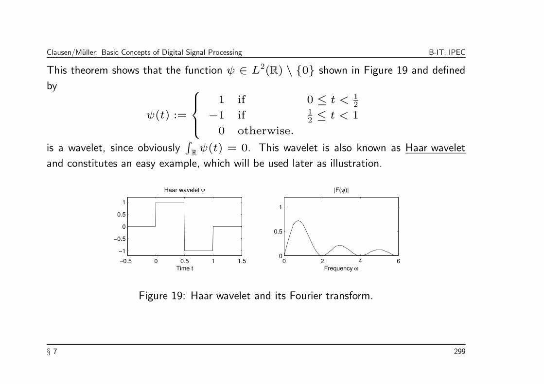
Clausen/Muller: Basic Concepts of Digital Signal Processing B-IT, IPEC
This theorem shows that the function ψ ∈ L2(R) \ 0 shown in Figure 19 and defined
by
ψ(t) :=
1 if 0 ≤ t < 12
−1 if 12 ≤ t < 1
0 otherwise.
is a wavelet, since obviously∫
Rψ(t) = 0. This wavelet is also known as Haar wavelet
and constitutes an easy example, which will be used later as illustration.
−0.5 0 0.5 1 1.5
−1
−0.5
0
0.5
1
Time t
Haar wavelet ψ
0 2 4 60
0.5
1
Frequency ω
|F(ψ)|
Figure 19: Haar wavelet and its Fourier transform.
§ 7 299

Clausen/Muller: Basic Concepts of Digital Signal Processing B-IT, IPEC
Theorem 7.5. Suppose φ ∈ L2(R) is continuously differentiable with
ψ := φ′ ∈ L
2(R) \ 0.
Then ψ is a wavelet.
As application of this theorem, we consider the so-called Mexican hat ψ : R → R shown
in Figure 20 and defined by
ψ(t) := − d2
dt2e−t22 = (1 − t
2)e
−t22 .
Obviously, the function φ : R → R defined by
φ(t) := − d
dte−t22
satisfies the conditions in Theorem 19. The function φ is, up to a sign, the derivative of
the Gauss function.
§ 7 300

Clausen/Muller: Basic Concepts of Digital Signal Processing B-IT, IPEC
−2 0 2−0.5
0
0.5
1
Time t
Mexican hat wavelet ψ
0 0.2 0.4 0.6 0.8 10
0.5
1
1.5
2
Frequency ω
|F(ψ)|
Figure 20: Mexican hat wavelet and its Fourier transform.
The illustration of ψ (up to a normalizing factor) in Figure 20 tells, how this wavelet came
to its name. In contrast to the Haar wavelet, the Mexican hat wavelet is a C∞-function
and has a much better localization property in the frequency domain.
§ 7 301

Clausen/Muller: Basic Concepts of Digital Signal Processing B-IT, IPEC
As another example, we introduce the so-called Meyer wavelet which is shown in Figure
21.
−5 0 5−1
−0.5
0
0.5
1
1.5
Time t
Meyer wavelet ψ
0 0.5 1 1.5 20
0.5
1
Frequency ω
|F(ψ)|
Figure 21: Meyer wavelet and its Fourier transform.
§ 7 302

Clausen/Muller: Basic Concepts of Digital Signal Processing B-IT, IPEC
The Meyer wavelet ψ is defined by means of its Fourier transform ψ. Let
ψ(y) :=1√2πeiy2 (w(y) + w(−y))
with
w(y) :=
sin(π2ν(3y
2π − 1))
if 2π3 ≤ y < 4π
3 ,
cos(π2ν(3y
2π − 1))
if 4π3 ≤ y < 2π,
0 otherwise,
where ν : R → [0, 1] is a smooth function such that ν(y) = 0 for y ≤ 0, ν(y) = 1
for y ≥ 1, and ν(y) + ν(1 − y) = 1. The admissibility condition for ψ follows from
the explicit formula of ψ.
§ 7 303
Clausen/Muller: Basic Concepts of Digital Signal Processing B-IT, IPEC
Note 7.6. Up to now, we gave examples for wavelets which were all given by explicit
formulas. However, for many of the common wavelets such explicit formulas do not
exist. In most cases, wavelets are implicitly defined by means of the so-called associated
filter coefficients which will be introduced in Chapter 8. The wavelets can then be
constructed from these filter coefficients by means of some recursive algorithm.
One important class of such implicitly defined wavelets are the Daubechies wavelets. Due
to their central importance in the theory of wavelets, we have illustrated the first five
wavelets of this family in Figure 22.
§ 7 304

Clausen/Muller: Basic Concepts of Digital Signal Processing B-IT, IPEC
0 0.2 0.4 0.6 0.8 1−2
0
2Daubechies wavelet dbN
db1
0 2 4 60
0.5
1|F(dbN)|
0 1 2 3−2
0
2
db2
0 2 4 60
0.5
1
0 1 2 3 4 5−2
0
2
db3
0 2 4 60
0.5
1
0 2 4 6−2
0
2
db4
0 2 4 60
0.5
1
0 2 4 6 8−2
0
2
db5
0 2 4 60
0.5
1
Figure 22: Daubechies wavelets and their corresponding Fourier transform.
§ 7 305

Clausen/Muller: Basic Concepts of Digital Signal Processing B-IT, IPEC
The family of Daubechies wavelets is parameterized by N ∈ N, where the Nth wavelet
is denoted by dbN . The wavelet db1 is just the Haar wavelet from Figure 19. All other
Daubechies wavelets do not have explicit formulas. As is illustrated by Figure 22, the
regularity of the wavelets dbN (e.g., in the sense of differentiability or in the sense of
localization property in the frequency domain) increases with increasing N . The wavelet
dbN has compact support [0, 2N − 1].
For a definition of the wavelets and further properties wie refer to [Strang/Nguyen].
§ 7 306

Clausen/Muller: Basic Concepts of Digital Signal Processing B-IT, IPEC
7.3 Time-frequency localization of the CWT
In a similar fashion as in Section 3 for the WFT we now want to investigate the
time-frequency representation f(s, t) of the CWT. In the following, let f ∈ L2(R) be a
signal and ψ ∈ L2(R) a wavelet with ||ψ|| = 1. As in Subsection 1, t0(ψ) denotes the
center and T (ψ) the width of ψ. Similarly, ω0(ψ) denotes the center and Ω(ψ) the
width of ψ. We assume that all values are finite. Then, as in Subsection 2, the inner
products
〈f |ψ〉can be interpreted as time-frequency analysis of f over the information cell IC(ψ) given
by the parameters t0(ψ), ω0(ψ), T (ψ) and Ω(ψ).
§ 7 307

Clausen/Muller: Basic Concepts of Digital Signal Processing B-IT, IPEC
The following theorem tells, how the information cell IC(ψ) behaves under translation
and scaling of the wavelet ψ.
Theorem 7.7. Let ψ be a wavelet with ||ψ|| = 1 and finite information cell IC(ψ).
Then for all t, s ∈ R, s 6= 0, holds
t0(ψs,t
) = s · t0(ψ) + t and T (ψs,t
) = |s| · T (ψ), (15)
as well as
ω0(ψs,t
) =1
sω0(ψ) and Ω(ψ
s,t) =
1
|s|Ω(ψ). (16)
§ 7 308

Clausen/Muller: Basic Concepts of Digital Signal Processing B-IT, IPEC
Proof: Using ||ψ|| = ||ψs,t||, the assertions follow by some straightforward substitution.
We just prove the assertion for t0(ψs,t) and leave the other cases as exercise.
t0(ψs,t
) =
∫
R
u|ψs,t(u)|2du
=1
|s|
∫
R
u
∣∣∣∣ψ(u− t
s
)∣∣∣∣2
du
=1
|s|
∫
R
(vs+ t)|ψ(v)|2 · |s|dv
= s
∫
R
v|ψ(v)|2dv + t||ψ||2
= s · t0(ψ) + t
§ 7 309

Clausen/Muller: Basic Concepts of Digital Signal Processing B-IT, IPEC
The width of the information cell IC(ψ) w.r.t. time is proportional to the scaling
parameter s, whereas w.r.t. frequency it is reciprocal to s. Hence, the shape of the
information cells for a CWT depends on s whereas the area is invariant under scaling and
translation. This is also illustrated by Figure 23.
t t+st0 0
ψ
ψ s,t
IZ( )
IZ( )ω0
ω0
__1S
Figure 23: Information cells for ψ and ψs,t with s = 12.
§ 7 310

Clausen/Muller: Basic Concepts of Digital Signal Processing B-IT, IPEC
We want to get an intuitive idea of this result.
• The scaling of a wavelet by a factor s > 0 is nothing else then compressing (s < 1)
or expanding (s > 1) the wavelet.
• For increasing s the wavelet ψs,t is expanded and the corresponding frequency
spectrum is compressed. Intuitively, the number of oscillations per time unit decreases
when stretching the wavelet.
• Contrary, for decreasing s the wavelet ψs,t is compressed and the corresponding
frequency spectrum is extended. Intuitively, the number of oscillations per time unit
increases when compressing the wavelet.
§ 7 311

Clausen/Muller: Basic Concepts of Digital Signal Processing B-IT, IPEC
These phenomena are reflected by the information cells. For a large parameter s, the
information cell IC(ψs,t) is wide-stretched in time having width sT and center t + st0and pressed in frequency having width 1
sΩ and center 1sω0.
In other words,
• for large s the inner products 〈f |ψs,t〉 analyze f w.r.t. long time segments and low
frequencies picking up global and low-frequency changes in f .
• For small s the inner product 〈f |ψs,t〉 analyze f w.r.t. short time segments and
high frequencies picking up sudden events of f such as peaks and high-frequency
oscillations.
Principle: The scaling factor s is reciprocal to the frequency parameter ω. If the note ψ
has pitch (i.e., frequency) ω0, the note ψs,t has frequencyω0s .
§ 7 312

Clausen/Muller: Basic Concepts of Digital Signal Processing B-IT, IPEC
Note 7.8. The above definition of localization in the frequency domain at ω0 is not
suitable for many wavelet transforms since for many common wavelets, ψ is an even
(symmetric) function which have a peak at some positive and at the corresponding
negative frequency. Therefore, let
ω+0 :=
∫ ∞
0
ω|ψ(ω)|2dω und ω−0 :=
∫ 0
−∞ω|ψ(ω)|2dω.
Then, we say that ψ localizes at (t0, ω±0 ). The parameter ω±
0 behaves under translation
and scaling of the wavelet just as ω0 and the interpretation remains the same. For further
details we refer to [Louis/Maaß/Rieder, p.31].
§ 7 313

Clausen/Muller: Basic Concepts of Digital Signal Processing B-IT, IPEC
7.4 Examples of some CWTs
7.4.1 CWT of some Chirp Signal
Figure 24 shows the time-scale representation of the CWT of a chirp signal f using a
db4-wavelet. The representation is analogous to the time-frequency representation of the
WFT in Subsection 6.2.2. The point at (t, s) has a gray color which is proportional to
the values
|f(s, t)| = |〈f |ψs,t〉|,
i.e., the larger the value the darker the color.
§ 7 314

Clausen/Muller: Basic Concepts of Digital Signal Processing B-IT, IPEC
100 200 300 400 500 600 700 800 900 1000−1
01
Chirp function f(t)=sin(400π (t/1000)2) and CWT with db4 wavelet (scale axis linear in s)
Zeit t in 1/1000
s ω
1000167916348383228242220181615141312121110
100 200 300 400 500 600 700 800 900 1000 1 6111621263136414651566166717681869196
Figure 24: Time-scale representation of the CWT of some chirp function.
§ 7 315

Clausen/Muller: Basic Concepts of Digital Signal Processing B-IT, IPEC
As was shown in the last section, the scaling parameter s is antiproportional to the
analyzed frequency ω. Since the chirp function has low frequencies for small points of
time t, there is a strong correlation between the wavelets ψs,t with large scaling parameter
s. Therefore, one has in Figure 24 dark points for small t and large s. With increasing
time t the frequency ω of the chirp signal also increases. So, one expects large values
|〈f |ψs,t〉| for decreasing s. Since the frequency of the chirp signal f increases linearly,
there is a hyperbola like shaped dark area in the time-scale representation of f .
In Figure 24, the frequencies ω corresponding to s are shown at the right hand side of the
time-scale representation. For a better comparison to the time-frequency representation
(such as in the figures 13 Figure 16 of the WFT) we have reparameterized the scale
axis such that the corresponding frequencies are linearly arranged (amounting to a
hyperbola-like arrangement of the scale axis). This is shown in Figure 25. In this figure
one again recognizes the diagonal analogously to the time-frequency representation of the
WFT of Figure 13.
§ 7 316

Clausen/Muller: Basic Concepts of Digital Signal Processing B-IT, IPEC
100 200 300 400 500 600 700 800 900 1000−1
01
Chirp function f(t)=sin(400π (t/1000)2) and CWT with db4 wavelet (scale axis linear in ω)
Time t in 1/1000
s ω
1
30
60
90
120
150
180
210
240
270
300
330
360
390
420
450
480
100 200 300 400 500 600 700 800 900 1000 1000
33.33333
16.66667
11.11111
8.333333
6.666667
5.555556
4.761905
4.166667
3.703704
3.333333
3.030303
2.777778
2.564103
2.380952
2.222222
2.083333
Figure 25: Reparameterized time-scale representation of Figure 24.
§ 7 317
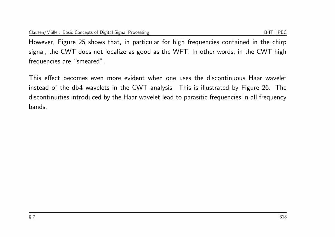
Clausen/Muller: Basic Concepts of Digital Signal Processing B-IT, IPEC
However, Figure 25 shows that, in particular for high frequencies contained in the chirp
signal, the CWT does not localize as good as the WFT. In other words, in the CWT high
frequencies are “smeared”.
This effect becomes even more evident when one uses the discontinuous Haar wavelet
instead of the db4 wavelets in the CWT analysis. This is illustrated by Figure 26. The
discontinuities introduced by the Haar wavelet lead to parasitic frequencies in all frequency
bands.
§ 7 318
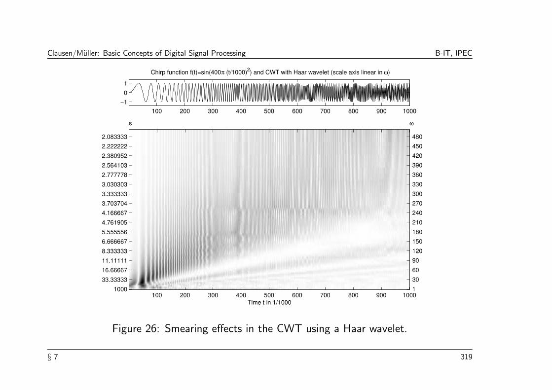
Clausen/Muller: Basic Concepts of Digital Signal Processing B-IT, IPEC
100 200 300 400 500 600 700 800 900 1000−1
01
Chirp function f(t)=sin(400π (t/1000)2) and CWT with Haar wavelet (scale axis linear in ω)
Time t in 1/1000
s ω
1
30
60
90
120
150
180
210
240
270
300
330
360
390
420
450
480
100 200 300 400 500 600 700 800 900 1000 1000
33.33333
16.66667
11.11111
8.333333
6.666667
5.555556
4.761905
4.166667
3.703704
3.333333
3.030303
2.777778
2.564103
2.380952
2.222222
2.083333
Figure 26: Smearing effects in the CWT using a Haar wavelet.
§ 7 319

Clausen/Muller: Basic Concepts of Digital Signal Processing B-IT, IPEC
7.4.2 CWT of Sines with Impulses.
Analogous to the last subsection, Figure 27 shows the time-scale representation of the
CWT w.r.t. the db4. This time the input signal is the superposition of two sines of
frequency ω1 = 10 and ω2 = 50, respectively, and two additional impulses at t1 = 0.4
and t2 = 0.5. Figure 28 shows the reparameterized time-scale representation with a linear
arrangement of the frequencies.
As in the time-frequency representation in Figure 16 one would expect two horizontal
stripes corresponding to the two frequencies ω1 and ω2 of the sines. In Figure 27 this two
stripes can be recognized — at least with some imagination — at the scale parameters
around s = 100 and s = 20 which corespond to the frequencies ω1 = 10 and ω2 = 50.
Also, the impulses can be recognized for small scale parameters s corresponding to high
frequencies.
§ 7 320

Clausen/Muller: Basic Concepts of Digital Signal Processing B-IT, IPEC
100 200 300 400 500 600 700 800 900 1000−2
02468
f(t)=sin(20π (t/1000))+sin(100π (t/1000)) with impulses at t=0.4 and t=0.5 and CWT with dpb4 wavelet
Time t in 1/1000
s ω
1000914832242016141211109887766
100 200 300 400 500 600 700 800 900 1000 1 11 21 31 41 51 61 71 81 91
101111121131141151161171
Figure 27: Time-scale representation of the CWT w.r.t. the db4 wavelet.
§ 7 321

Clausen/Muller: Basic Concepts of Digital Signal Processing B-IT, IPEC
100 200 300 400 500 600 700 800 900 1000−2
02468
f(t)=sin(20π (t/1000))+sin(100π (t/1000)) with impulses at t=0.4 and t=0.5 and CWT with db4 wavelet
Time t in 1/1000
s ω
1306090120150180210240270300330360390420450480
100 200 300 400 500 600 700 800 900 1000 1000
33.3333316.6666711.111118.3333336.6666675.5555564.7619054.1666673.7037043.3333333.0303032.7777782.5641032.3809522.2222222.083333
Figure 28: Reparameterized time-scale representation of Figure 27.
§ 7 322

Clausen/Muller: Basic Concepts of Digital Signal Processing B-IT, IPEC
Note that the two horizontal stripes of Figure 27 and Figure 28, which correspond to the
frequencies ω1 and ω2 of the sines, are smeared in frequency. Furthermore, these stripes
are periodically interrupted by “vertical white stripes”. In the following we give some
explanation of such phenomena.
To this means, we fix a scale parameter s = s0 and a point of time t = t1 so that the
absolute value of the wavelet coefficient 〈f |ψs0,t1〉 is large as, e.g., for s0 = 100 and
t1 = 0.575. The wavelet ψs0,t1 and the function f have then a high correlation at
t0(ψs0,t1) = t1. In other words, f and ψs0,t1 have the same sign at most points, i.e.,
ψs0,t1 “nestles” against the function f (in our case against the low-frequency osciallation
ω1 = 10 of f). This leads to a large wavelet coefficient 〈f |ψs0,t1〉. Figure 29 (a)
illustrates this situation.
§ 7 323

Clausen/Muller: Basic Concepts of Digital Signal Processing B-IT, IPEC
Next, we look at the point of time t2 = 0.625 which corresponds to a translation of the
wavelet ψs0,t1 of half a period of the sine of frequency ω1 = 10. Then, ψs0,t2 and f
have opposite sign at most points as is illustrated in Figure 29 (b). Again the absolute
value of the wavelet coefficient 〈f |ψs0,t2〉 is large. However, 〈f |ψs0,t2〉 and 〈f |ψs0,t1〉have opposite sign.
Now, it is not difficult to see that the function t 7→ 〈f |ψs0,t〉 is continuous, which
assumes positive values (such as for t = t1) as well as negative values (such as for
t = t2). Therefore, this function has a zero at some point of time tzero between t1 and
t2. This is illustrated by Figure 29 (c).
This explains the periodic interruption by “vertical white stripes” (corresponding to
neighborhoods of the zeros). Note that this periodic interruption takes place two times
the period ω = 10 of the low-frequency sine component of f .
§ 7 324

Clausen/Muller: Basic Concepts of Digital Signal Processing B-IT, IPEC
−2 −1 0 1 2 3 4 5
−1
−0.5
0
0.5
1
Wavelet ψs0,t and signal f (dotted)
(a)(a)(a)(a)
−2 −1 0 1 2 3 4 5
−1
−0.5
0
0.5
1
(b)(b)(b)(b)
−2 −1 0 1 2 3 4 5
−1
−0.5
0
0.5
1
(c)(c)(c)(c)
Figure 29: Strong positive (a), negative (b), and weak (c) correlation of the wavelets
ψs0,t with the signal f .
§ 7 325

Clausen/Muller: Basic Concepts of Digital Signal Processing B-IT, IPEC
7.4.3 Reconstruction of the Signal from its CWT
Let f ∈ L2(R) be a signal with CWT f(s, t) w.r.t. a wavelet ψ ∈ L2(R) having
admissability constant
0 < cψ :=
∫
R
|ψ(ω)|2|ω| dω < ∞.
In this section, we want to reconstruct the signal f from its CWT. Recall that, as explained
in Section 7.3, the wavelet coefficient f(s, t) can be interpreted as the intensity in which
the note ψs,t is contained in the signal f . If the note ψ is of frequency ω0, the note ψs,t
has frequencyω0s . Intuitively, the signal f should be representable as a superposition of
the notes ψω0ω ,t of frequency ω weighted by f(
ω0ω , t):
f(u) ∼∫
R
∫
R
f
(ω0
ω, t
)ψω0ω ,t
(u)dωdt = ω0
∫
R
∫
R
f(s, t)ψs,t
(u)1
s2dsdt,
where the last equation follows by the substitution s =ω0ω . We will see that this
reconstruction formula holds up to a constant normalizing factor.
§ 7 326

Clausen/Muller: Basic Concepts of Digital Signal Processing B-IT, IPEC
In the following computations we need the Fourier transform ψs,t of ψs,t. By (13) of
Theorem 7.2 holds
ψs,t(ω) = e−2πiωt|s|12ψ(sω). (17)
Using this formula we obtain by Parseval’s equality
f(s, t) = 〈f |ψs,t〉 = 〈f |ψs,t〉
=
∫
R
|s|12e−2πiωtψ(sω)f(ω)dω (18)
= |s|12(ψ(s·)f(·)
)∨(t).
Applying the Fourier transform on both sides one gets
∫
R
e−2πiωt
f(s, t)dt = |s|12ψ(sω)f(ω) (19)
§ 7 327
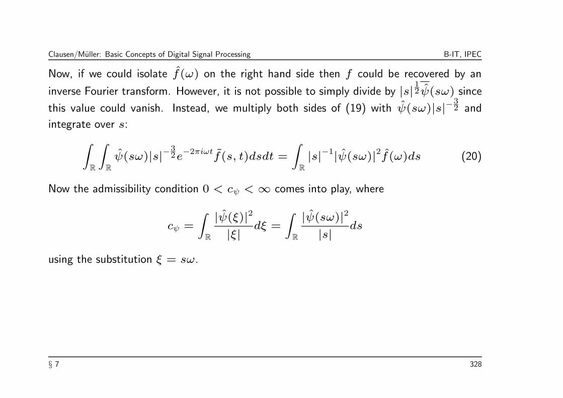
Clausen/Muller: Basic Concepts of Digital Signal Processing B-IT, IPEC
Now, if we could isolate f(ω) on the right hand side then f could be recovered by an
inverse Fourier transform. However, it is not possible to simply divide by |s|12ψ(sω) since
this value could vanish. Instead, we multiply both sides of (19) with ψ(sω)|s|−32 and
integrate over s:
∫
R
∫
R
ψ(sω)|s|−32e
−2πiωtf(s, t)dsdt =
∫
R
|s|−1|ψ(sω)|2f(ω)ds (20)
Now the admissibility condition 0 < cψ < ∞ comes into play, where
cψ =
∫
R
|ψ(ξ)|2|ξ| dξ =
∫
R
|ψ(sω)|2|s| ds
using the substitution ξ = sω.
§ 7 328

Clausen/Muller: Basic Concepts of Digital Signal Processing B-IT, IPEC
Dividing both sides of (20) by cψ and using (17) one gets the following reconstruction
formula of f :
f(ω) =1
cψ
∫
R
∫
R
f(s, t)ψ(sω)|s|−32e
−2πiωtdsdt
=1
cψ
∫
R
∫
R
f(s, t)ψs,t(ω)|s|−2dsdt. (21)
Applying the inverse Fourier transform one obtains the reconstruction formula of the signal
f :
f(u) =1
cψ
∫
R
∫
R
∫
R
f(s, t)ψs,t(ω)e2πiωu 1
s2dωdsdt
=1
cψ
∫
R
∫
R
f(s, t)ψs,t
(u)1
s2dsdt. (22)
§ 7 329

Clausen/Muller: Basic Concepts of Digital Signal Processing B-IT, IPEC
The result is summarized in the following theorem.
Theorem 7.9. Let ψ be a wavelet, i.e., ψ ∈ L2(R) satisfying the admissability condition
0 < cψ :=
∫
R
|ψ(ξ)|2|ξ| dξ < ∞.
Then any signal f ∈ L2(R) can be reconstructed from its CWT f(s, t) by
f(u) =1
cψ
∫
R
∫
R
f(s, t)ψs,t
(u)1
s2dsdt.
§ 7 330
Clausen/Muller: Basic Concepts of Digital Signal Processing B-IT, IPEC
7.5 Discrete Version of the CWT
In the previous sections we have introduced the continuous version of the wavelet
transform. This case is important in order to get the “right” intuition of how to interpret
wavelet coefficients. In the following we discuss some of the problems which arise when
one actually wants to compute the wavelet transform. Thus we are faced with the
questions of
(1) how to discretize the continuous wavelet transform,
(2) how to compute this discretized wavelet transform efficiently, and
(3) how to compute the reconstruction of a signal from its discretized wavelet transform
(inversion) efficiently.
§ 7 331

Clausen/Muller: Basic Concepts of Digital Signal Processing B-IT, IPEC
7.5.1 CWT-Adapted Grid
By Theorem 7.9, a signal f ∈ L2(R) can by reconstructed by the synthesis formula
f(u) =1
cψ
∫
R
∫
R
f(s, t)ψs,t
(u)1
s2dsdt,
f is the CWT w.r.t. some wavelet ψ. As discussed in Section 6.4 for the WFT, this
representation is in general rather redundant: a one-dimensional parameter space (the time
denoted by the variable u) is represented by an integral over a two-dimensional parameter
space (the time-scale domain represented by the variables t and s). In the following,
we discuss a discrete version of the CWT where a discrete (or even finite) set of values
f(s, t) is sufficient for the reconstruction of the signal f .
Warning: The word “discrete” does not refer to the wavelet itself, which always will be
a time-continuous function in L2(R). It refers to the discrete number of points in the
time-scale parameter space on which the CWT is evaluated.
§ 7 332

Clausen/Muller: Basic Concepts of Digital Signal Processing B-IT, IPEC
Of course, the discrete subset in R \ 0 × R on which the CWT is to be evaluated
depends on the wavelet. For example, in the case of the discrete version of the WFT
in Section 6.4, where we only considered window functions with compact support, the
mesh of the discrete grid in the time-frequency plane depended on the respective window
function.
A similar assertion holds for the CWT. However, in this case we do not consider an
equidistant grid, but a grid of the form
(am, nbam)|m,n ∈ Z ⊂ R \ 0 × R (23)
with a > 1, b > 0 and the corresponding set of functions
ψ
(a,b)m,n := ψ
am,nbam= a
−m/2ψ(a
−m · −nb)|m,n ∈ Z
.
§ 7 333

Clausen/Muller: Basic Concepts of Digital Signal Processing B-IT, IPEC
The form of this grid is motivated by the time-frequency interpretation of the CWT in
Section 7.3. Let ψ be a wavelet with ||ψ|| = 1 and let IC(ψ) be the corresponding
information cell with center (t0(ψ), ω0(ψ)), width T (ψ), and height Ω(ψ). We consider
the case t0 = 0 und ω0 > 0. Then, by Equation (15), the center of the information cell
IC(ψa,bm,n) of the note ψa,bm,n is given by
(a−mω0, nba
m)
and, by Equation (16), the width and height are given by
T (ψ(a,b)m,n ) = a
mT (ψ) bzw. Ω(ψ
(a,b)m,n ) = a
−mΩ(ψ).
With increasing frequency (m → −∞) the time component of the centers of the
functions ψ(a,b)m,n |n ∈ Z are closer together. This is also illustrated by Figure 30).
Therefore, the grids as defined by Equation (23) model the zoom effect of the CWT.
§ 7 334

Clausen/Muller: Basic Concepts of Digital Signal Processing B-IT, IPEC
ω
ω0
0
/a ab
aω0
ω
t
Figure 30: Distribution of the points (nbam, a−mω0) for a = 2 and b = 1 in the
time-frequency plane.
§ 7 335
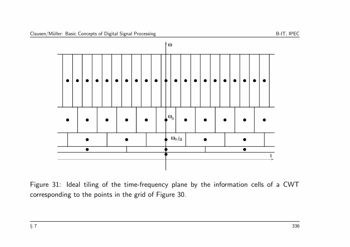
Clausen/Muller: Basic Concepts of Digital Signal Processing B-IT, IPEC
ω0 /a
t
ω
ω0
Figure 31: Ideal tiling of the time-frequency plane by the information cells of a CWT
corresponding to the points in the grid of Figure 30.
§ 7 336
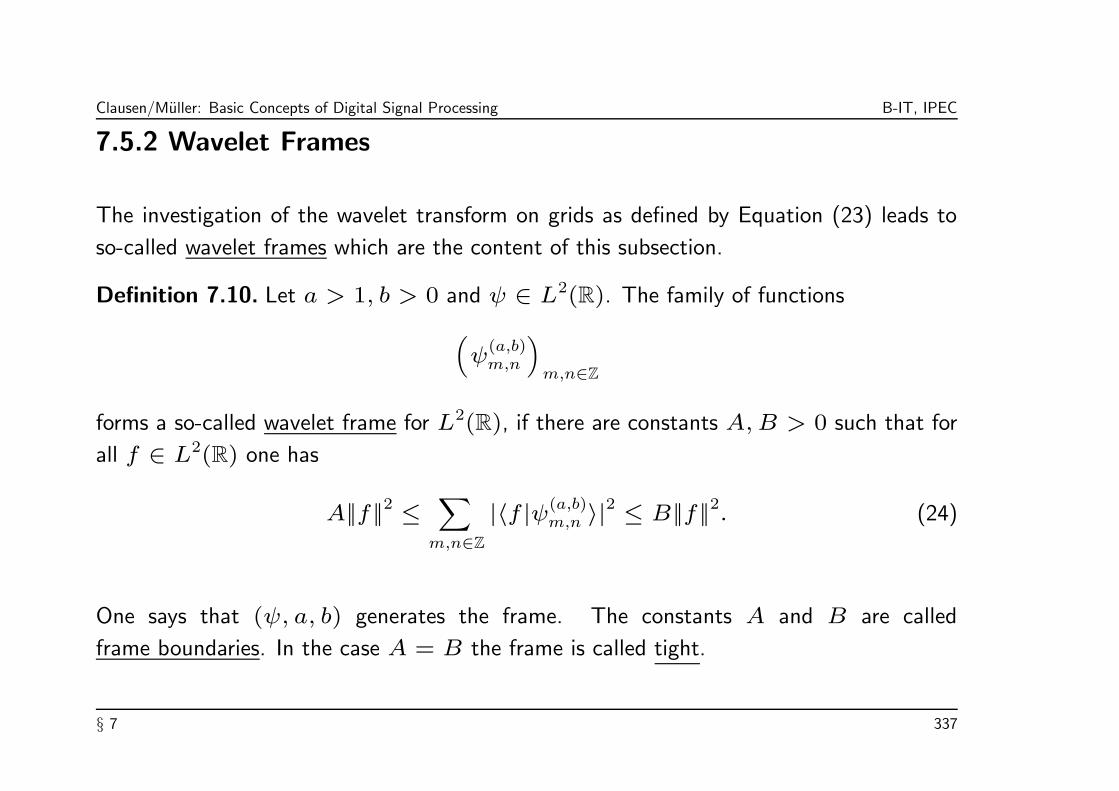
Clausen/Muller: Basic Concepts of Digital Signal Processing B-IT, IPEC
7.5.2 Wavelet Frames
The investigation of the wavelet transform on grids as defined by Equation (23) leads to
so-called wavelet frames which are the content of this subsection.
Definition 7.10. Let a > 1, b > 0 and ψ ∈ L2(R). The family of functions
(ψ
(a,b)m,n
)m,n∈Z
forms a so-called wavelet frame for L2(R), if there are constants A,B > 0 such that for
all f ∈ L2(R) one has
A||f ||2 ≤∑
m,n∈Z
|〈f |ψ(a,b)m,n 〉|2 ≤ B||f ||2. (24)
One says that (ψ, a, b) generates the frame. The constants A and B are called
frame boundaries. In the case A = B the frame is called tight.
§ 7 337

Clausen/Muller: Basic Concepts of Digital Signal Processing B-IT, IPEC
The next theorem shows that the concept of wavelet frames generalizes the concept of
ON bases.
Theorem 7.11. A tight wavelet frame (ψ, a, b) with frame boundaries A = B = 1
and ||ψ|| = 1 forms an ON basis L2(R).
Proof: Let (ψ, a, b) be a tight wavelet frame. Then
||ψ(a,b)m,n || = ||ψ|| = 1
for all m,n ∈ Z. Since A = B = 1, one has equality in (24) and setting f = ψ(a,b)µ,ν ,
µ, ν ∈ Z, one gets
||ψ(a,b)µ,ν ||2 =
∑
m,n∈Z
|〈ψ(a,b)µ,ν |ψ(a,b)
m,n 〉|2
= ||ψ(a,b)µ,ν ||2 +
∑
m,n∈Z,(m,n)6=(µ,ν)
|〈ψ(a,b)µ,ν |ψ(a,b)
m,n 〉|2
§ 7 338

Clausen/Muller: Basic Concepts of Digital Signal Processing B-IT, IPEC
Therefore, it follows that 〈ψ(a,b)µ,ν |ψ(a,b)
m,n 〉 = 0 for (m,n) 6= (µ, ν). This proves the
orthonormality. Completeness of the family follows from Parseval’s equation and (24) with
A = B = 1.
In general, it can be rather difficult to prove if the frame conditions are fulfilled or not.
For sufficient conditions we refer to [Louis/Maaß/Rieder]. In this book it is also shown
that the Meyer wavelet ψ (see Figure 21) forms a tight wavelet frame with a = 2 and
b = 1. Then, Theorem 7.11 implies the following result.
Corollary 7.12. The Meyer wavelet ψ generates a frame (ψ, 2, 1) which forms an ON
basis of L2(R).
§ 7 339

Clausen/Muller: Basic Concepts of Digital Signal Processing B-IT, IPEC
Each wavelet frame (ψ, a, b) defines a linear operator
T : L2(R) → `(Z × Z)
f 7→ (〈f |ψ(a,b)m,n 〉)m,n∈Z.
This operator fulfills
A12||f ||L2 ≤ ||Tf ||`2 ≤ B
12||f ||L2. (25)
Therefore, T is continuous since its norm is bounded by
||T || := sup||f ||=1
||Tf || ≤ B12.
§ 7 340

Clausen/Muller: Basic Concepts of Digital Signal Processing B-IT, IPEC
Furthermore, from A > 0 follows that T is injective and continuously invertible on its
image since
||T−1|ImageT || ≤ A−1
2.
In this case f can be reconstructed from the discrete set of values
Tf = (〈f |ψ(a,b)m,n 〉)m,n∈Z.
Next, we explain how this reconstruction can be achieved in a more general framework. let
H be a (separable) Hilbert space and Φ = (ϕj)j∈Z a frame, i.e.,
∃A,B > 0∀v ∈ H : A||v||2 ≤∑
j∈Z
|〈v|ϕj〉|2 ≤ B||v||2. (26)
For given Φ we define the frame operator S : H → H by
Sv :=2
A+ B
∑
j∈Z
〈v|ϕj〉ϕj.
§ 7 341
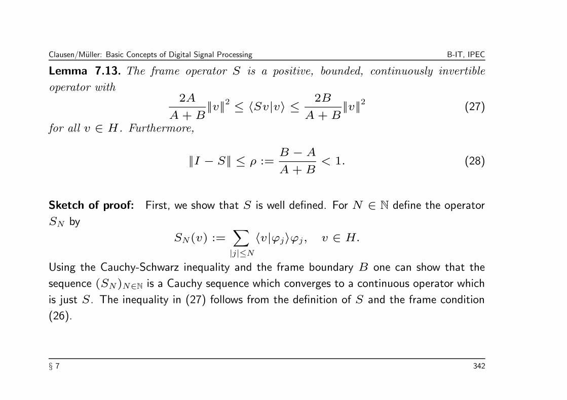
Clausen/Muller: Basic Concepts of Digital Signal Processing B-IT, IPEC
Lemma 7.13. The frame operator S is a positive, bounded, continuously invertible
operator with2A
A+ B||v||2 ≤ 〈Sv|v〉 ≤ 2B
A+ B||v||2 (27)
for all v ∈ H. Furthermore,
||I − S|| ≤ ρ :=B − A
A+ B< 1. (28)
Sketch of proof: First, we show that S is well defined. For N ∈ N define the operator
SN by
SN(v) :=∑
|j|≤N〈v|ϕj〉ϕj, v ∈ H.
Using the Cauchy-Schwarz inequality and the frame boundary B one can show that the
sequence (SN)N∈N is a Cauchy sequence which converges to a continuous operator which
is just S. The inequality in (27) follows from the definition of S and the frame condition
(26).
§ 7 342

Clausen/Muller: Basic Concepts of Digital Signal Processing B-IT, IPEC
Now, we show (28). From (27) follows
(1 − 2B
A+ B
)||v||2 ≤ 〈(I − S)v|v〉 ≤
(1 − 2A
A+ B
)||v||2
and therefore
|〈(I − S)v|v〉| ≤ B − A
A+ B||v||2 = ρ||v||2.
From this follows (28) using the well-known fact from functional analysis that
||I − S|| = sup||v||=1
|〈(I − S)v|v〉|.
For further details we refer to the literature.
§ 7 343

Clausen/Muller: Basic Concepts of Digital Signal Processing B-IT, IPEC
Important for the construction of the inverse S−1 of S is property (28). Since ρ < 1, the
so-called Neumann series∞∑
k=0
(I − S)k
converges towards S−1. Therefore, the sequence
vn :=
n∑
k=0
(I − S)kSv
converges to v. Furthermore, (vn)n∈N satisfies the recursion
vn+1 = Sv + (I − S)
n+1∑
k=1
(I − S)(k−1)
Sv = Sv + (I − S)vn (29)
and the error estimate
||v − vn|| = ||(I − S)n+1
v|| ≤ ρn+1||v||. (30)
§ 7 344

Clausen/Muller: Basic Concepts of Digital Signal Processing B-IT, IPEC
The recursion (29) is a common algorithm for the approximation of S−1. If the frame
boundaries A and B are close together, i.e., B/A ≈ 1, then ρ ≈ 0 and only a few steps
in the recursion are sufficient to guarantee a good approximation of v.
§ 7 345

Clausen/Muller: Basic Concepts of Digital Signal Processing B-IT, IPEC
We come back to our specific situation. We have discussed that there exists wavelet
frames (ψ, a, b) and that in this case a signal f ∈ L2(R) can be perfectly recovered
from ths wavelet coefficients
f(a−m, nba
−m),m, n ∈ Z.
If one just uses a finite number of grid points (the grid points which correspond to
the “large” wavelet coefficients f(a−m0 , nb0am0 )), then at least an approximation of the
original signal f can be reconstructed from this finite set of wavelet coefficients. Then the
following primitive “algorithm” can be used to compute a discrete wavelet transform:
Pick a suitable wavelet frame (ψ, a, b) and compute some approximation of the wavelet
coefficients
f(am, nba
m) = 〈f |ψ(a,b)
m,n 〉for all “essential” grid points (a finite number). The approximation of the wavelet
coefficients could, for example, be done by computing suitable Riemann sums.
§ 7 346

Clausen/Muller: Basic Concepts of Digital Signal Processing B-IT, IPEC
This “algorithm” is in general neither efficient nor practicable.
• The approximation of the relevant integrals 〈f |ψ(a0,b0)n,m 〉 is rather expensive.
• Furthermore, the choice of the “essential” grid points depends on the signal to be
analyzed.
• It is not clear how to determine, a priori, which grid points turn out to be essential.
In the year 1986 the connection between the so-called multiresolution analysis and wavelet
transforms was discovered which led to completely new insights into the theory of wavelets.
Based on these ideas fast algorithms for the discrete wavelet transform as well as its
reconstruction were found. These recursive algorithms, which will be the content of the
next chapter, are well suited in view of efficient implementations.
§ 7 347

Clausen/Muller: Basic Concepts of Digital Signal Processing B-IT, IPEC
Chapter 8: Multiresolution Analysis (MRA) andWavelet Transform
Again we cite as an introduction Barbara Burke Hubbard who gives in [Hubbard] the
following nice account of multiresolution.
Coming from different directions — pure mathematics and computer vision — Stephane
Mallat und Yves Meyer created multiresolution theory. One result of their work was
the fast wavelet transform. Another result was a mathematical theory of orthogonal
wavelets. This theory defines four mathematical conditions which, if met, make it
possible to view a signal at resolutions differing by a factor of two, and to encode
the difference of information from one resolution to the next as orthogonal wavelet
coefficients.
§ 8 348

Clausen/Muller: Basic Concepts of Digital Signal Processing B-IT, IPEC
The theory also gives a recipe for creating new orthogonal wavelet bases. Both scaling
functions and wavelets can be created using a function that is the Fourier transform
of a low-pass filter. (In geometrical terms, this function parameterizes a curve on a
sphere in four-dimensional space.) Curiously, the bottom line of multiresolution theory
is that to compute the wavelet transform of a signal we need neither scaling functions
nor wavelets: just very simple digital filters.
In this chapter we first introduce the concept of multiresolution, describe their links
to wavelet theory, and then discuss the resulting fast wavelet algorithms (FDWT and
FIDWT).
§ 8 349

Clausen/Muller: Basic Concepts of Digital Signal Processing B-IT, IPEC
8.1 Multiresolution Analysis (MRA)
8.1.1 Motivating Analogy
We first want to illustrate the main idea of the multiresolution analysis (MRA) by means
of some MRA-like situation. We want to emphasize that this analogy only holds w.r.t.
some aspects of MRA and exclusively serves as motivation.
For this purpose, we consider the binary representation of a real number f ∈ R (the
symbol f should remind on a signal) in the following way. Let
Vm := 2m
Z for m ∈ Z.
§ 8 350

Clausen/Muller: Basic Concepts of Digital Signal Processing B-IT, IPEC
Then the following properties hold:
0 ⊂ . . . ⊂ V2 ⊂ V1 ⊂ V0 ⊂ V−1 ⊂ V−2 ⊂ . . . ⊂ R,
⋃
m∈Z
Vm = R,
⋂
m∈Z
Vm = 0,
f ∈ Vm ⇐⇒ f · 2−m ∈ V0.
§ 8 351

Clausen/Muller: Basic Concepts of Digital Signal Processing B-IT, IPEC
If the real number f has the binary representation
f =∑
n∈Z
wn2n, wn ∈ 0, 1,
then the “projection” Pif of f onto Vi is given by
Pif :=∑
n≥iwn2
n.
In other words, setting all digits of f up to position i − 1 to zero results in the number
Pif . Increasing i results in a “coarser resolution” Pif of f and, contrary, decreasing i
results in a “finer resolution”. In practice, the computation of the binary representation
(at least some approximation with some prescribed precision) is the goal. One starts
with some coarse approximation given by some Pif (often i = 0). The one computes
successively the numbers wn, n = i, i + 1, i + 2, . . .. Doing so, in each step from j to
j + 1 one records the “detail” wj2j, wj ∈ 0, 1.
§ 8 352
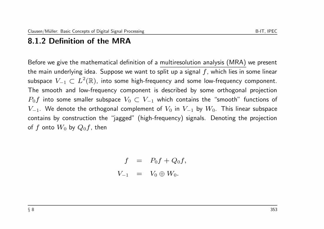
Clausen/Muller: Basic Concepts of Digital Signal Processing B-IT, IPEC
8.1.2 Definition of the MRA
Before we give the mathematical definition of a multiresolution analysis (MRA) we present
the main underlying idea. Suppose we want to split up a signal f , which lies in some linear
subspace V−1 ⊂ L2(R), into some high-frequency and some low-frequency component.
The smooth and low-frequency component is described by some orthogonal projection
P0f into some smaller subspace V0 ⊂ V−1 which contains the “smooth” functions of
V−1. We denote the orthogonal complement of V0 in V−1 by W0. This linear subspace
contains by construction the “jagged” (high-frequency) signals. Denoting the projection
of f onto W0 by Q0f , then
f = P0f +Q0f,
V−1 = V0 ⊕W0.
§ 8 353

Clausen/Muller: Basic Concepts of Digital Signal Processing B-IT, IPEC
Analogously, we proceed with P0f by splitting up V0 into some orthogonal sum of
subspaces V1 (“smooth” elements) and W1 (“jagged” elements). The respective
projections are denoted by P1 and Q1. Since P1P0f = P1f as well as Q1Q0f = Q1f
we get
P0f = P1f +Q1f
and therefore
f = P1f +Q1f +Q0f. (31)
Proceeding recursively, P1 is split up into P2f and Q2, and so on
L2(R) . . . −→ V−1P0−→ V0
P1−→ V1 . . . −→ 0Q0
Q1
. . . W0 W1 . . .
§ 8 354

Clausen/Muller: Basic Concepts of Digital Signal Processing B-IT, IPEC
The projections can be interpreted as follows:
• P1f represents the low-frequency components of f representing the details of f below
some specific size.
• Q0f and Q1f “contain” components of f corresponding to certain a frequency band
where Q0f represents higher-frequency details of f than Q1f .
• Equation (31) can be thought of as a decomposition of the signal corresponding to
frequency bands consisting of high frequencies components and a mixture of lower
frequencies.
For an illustration we refer to Figure 34 and Figure 35.
This decomposition process can mathematically modeled by the multiresolution analysis.
§ 8 355

Clausen/Muller: Basic Concepts of Digital Signal Processing B-IT, IPEC
Definition 8.1. A multiresolution analysis (MRA) of L2(R) is a sequence of closed
subspaces Vm ⊂ L2(R)
0 ⊂ . . . ⊂ V2 ⊂ V1 ⊂ V0 ⊂ V−1 ⊂ V−2 ⊂ . . . ⊂ L2(R), (32)
such that the following holds:
⋃
m∈Z
Vm = L2(R), (33)
⋂
m∈Z
Vm = 0, (34)
f(·) ∈ Vm ⇐⇒ f(2m·) ∈ V0. (35)
Furthermore, one postulates the existence of some function ϕ ∈ V0, the so-called
scaling function, whose integral translates form an ON-basis of V0, i.e.,
V0 = spanϕ(· − k)|k ∈ Z. (36)
§ 8 356

Clausen/Muller: Basic Concepts of Digital Signal Processing B-IT, IPEC
The easiest example for an MRA is the so-called Haar-MRA which will be presented in
Section 8.3 In the following we discuss Definition 8.1 and summarize some immediate
consequences.
(1) Conditions (33) and (34) are fulfilled by many families of subspaces (Vm)m∈Z. An
MRA is distinguished by Condition (35): the spaces Vm are scaled versions of the base
space V0, spanned by the translations of the scaling function ϕ (36).
(2) For increasing m (m → ∞) the functions in Vm become broad, details are bloat.
Contrary, when decreasing m (m → −∞), the functions in Vm become jagged
containing more and more details. Let Pm denote the orthogonal projector onto Vm.
Then the limits
limm→+∞
||Pmf || = 0 and limm→−∞
||Pmf − f || = 0
state this interpretation more precisely. One says that Pmf is the representation of f
on “scale” Vm and contains all details of f up to size 2m.
§ 8 357

Clausen/Muller: Basic Concepts of Digital Signal Processing B-IT, IPEC
(3) Because of Condition (36), the space V0 is translation invariant, i.e.,
f ∈ V0 ⇐⇒ f(· − k) ∈ V0 for k ∈ Z.
From (35) follows
f ∈ Vm ⇐⇒ f(· − 2mk) ∈ Vm for k ∈ Z.
(4) The space Vm is spanned by the functions
ϕm,k(x) := 2−m/2
ϕ(2−mx− k),
in fact, (ϕm,k)m∈Z is an ON-basis of Vm:
Vm = spanϕm,k|k ∈ Z.
This follows from (35) and (36). Furthermore holds ||ϕm,k|| = ||ϕ||.
§ 8 358
Clausen/Muller: Basic Concepts of Digital Signal Processing B-IT, IPEC
(5) In the definition of an MRA one often encounters the condition, that the translates of
the scaling function ϕ form a so-called Riesz basis. This seems to be a weaker condition
then the condition of forming an ON-basis as stated in Definition 8.1. However, one
can show that, starting with a Riesz basis, one can construct an ON-basis with the
same properties. Hence, our definition does not mean any restriction in generality.
§ 8 359

Clausen/Muller: Basic Concepts of Digital Signal Processing B-IT, IPEC
As in the introductory explanation of the main idea, we define the space Wm as the
orthogonal complement of Vm in Vm−1,
Vm−1 = Wm ⊕ Vm, Vm ⊥ Wm, (37)
and the operators Qm as orthogonal projection from L2(R) onto Wm,
Pm−1 = Qm + Pm. (38)
Then
Vm =⊕
j≥m+1
Wj and therefore L2(R) =
⊕
j∈Z
Wj. (39)
§ 8 360

Clausen/Muller: Basic Concepts of Digital Signal Processing B-IT, IPEC
The spaces Wm inherit the scaling property of the spaces Vm (see (35)):
f(·) ∈ Wm ⇐⇒ f(2m·) ∈ W0. (40)
Using Equation (39), one sees that a function f ∈ L2(R) can be decomposed as
f =∑
j∈Z
Qjf =∑
j≥m+1
Qjf +∑
j≤mQjf = Pmf +
∑
j≤mQjf. (41)
This decomposition of f explains the denotation of multiresolution analysis. Pmf
represents f on scale m, which corresponds to applying a low-pass filter on f having a
decreasing cut-off frequency for increasing m. The remaining high-frequency component
is split into various frequency bands Qjf,−∞ < j ≤ m. In doing so, Qj contains the
details by which Pj−1 differs from Pj:
Qj = Pj−1 − Pj.
§ 8 361

Clausen/Muller: Basic Concepts of Digital Signal Processing B-IT, IPEC
8.2 MRA und Wavelets
At first sight, there does not seem to be any connection between the definition of the
MRA and the wavelet theory introduced in the last chapter. We present the main result
of this section, which appears like a miracle:
Main Result: To each MRA there is a wavelet ψ whose translated and dilated versions
ψm,k(x) := 2−m/2
ψ(2−mx− k)
for a fixed m ∈ Z form an orthonormal basis (ONB) of the space Wm. Furthermore, the
wavelet can be constructed explicitly from the scaling function ϕ.
§ 8 362

Clausen/Muller: Basic Concepts of Digital Signal Processing B-IT, IPEC
Surprisingly, digital filters
(hk)k∈Z and (gk)k∈Z
come into play when constructing such a wavelet ψ from the scaling function ϕ of the
MRA. These filters do not only establish the connection between MRAs and wavelet theory
but also between time-continuous and time-discrete signal processing.
The following diagram give an overview:
§ 8 363

Clausen/Muller: Basic Concepts of Digital Signal Processing B-IT, IPEC
MRA Wavelets
((Vm), ϕ) ψ defines
ϕ ∈ V0 ⊂ V−1 a wavelet
⇓ ⇑Scaling equation Wavelet equation
ϕ =∑
k∈Zhkϕ−1,k ψ :=
∑k∈Z
gkϕ−1,k ∈ V−1
⇓ ⇑Scaling coefficients Wavelet coefficients
(hk)k∈Z ∈ `2(Z) =⇒ (gk)k∈Z ∈ `2(Z)
gk := (−1)kh1−k
Digital filters
§ 8 364

Clausen/Muller: Basic Concepts of Digital Signal Processing B-IT, IPEC
8.2.1 Filter Coefficients and Scaling Equation
By Definition 8.1 an MRA has a scaling function ϕ whose translates form on ON-basis
of the base space V0. In combination with the other axioms we derive in the following
further properties of ϕ.
Lemma 8.2. The scaling function ϕ satisfies the so-called scaling equation, i.e., there
is a sequence (hk)k∈Z of complex numbers with
ϕ(x) =√
2∑
k∈Z
hkϕ(2x− k). (42)
Proof: Noting the inclusion ϕ ∈ V0 ⊂ V−1 = span√
2ϕ(2 · −k)|k ∈ Z the lemma
follows immediately.
§ 8 365

Clausen/Muller: Basic Concepts of Digital Signal Processing B-IT, IPEC
Note 8.3. In the scaling equation
ϕ(x) =√
2∑
k∈Z
hkϕ(2x− k)
lies the key for the construction of orthonormal wavelet bases as well as for fast wavelet
algorithms. The coefficients
(hk)k∈Z
will come to the fore whereas the scaling function ϕ will only stay in the background.
§ 8 366

Clausen/Muller: Basic Concepts of Digital Signal Processing B-IT, IPEC
Lemma 8.4. The delated and translated versions ϕm,k of the scaling function ϕ satisfies
the scaling equation
ϕm,k =∑
j∈Z
hjϕm−1,2k+j. (43)
Proof: This follows directly from the scaling equation (42) and the definition of ϕm,k:
ϕm,k(x) = 2−m/2
ϕ(2−mx− k)
(42)= 2
−m/22
1/2∑
j∈Z
hjϕ(2(2−mx− k) − j)
= 2−(m−1)/2
∑
j∈Z
hjϕ(2−(m−1)
x− (2k + j))
=∑
j∈Z
hjϕm−1,2k+j(x).
§ 8 367

Clausen/Muller: Basic Concepts of Digital Signal Processing B-IT, IPEC
Lemma 8.5. The coefficients (hk)k∈Z of the scaling equation (42) satisfy the following
orthogonality relations: ∑
k∈Z
hk+2jhk = δ0,j. (44)
Proof: This follows directly from the orthogonality relations satisfied by the translates of
the scaling functions:
δ0,j = 〈ϕ(·)|ϕ(· + j)〉(43)= 〈
∑
l∈Z
hlϕ−1,l|∑
k∈Z
hkϕ−1,2j+k〉
=∑
l∈Z
∑
k∈Z
hlhk〈ϕ−1,l|ϕ−1,2j+k〉
=∑
l∈Z
∑
k∈Z
hlhkδl,k+2j =∑
k∈Z
hk+2jhk
§ 8 368

Clausen/Muller: Basic Concepts of Digital Signal Processing B-IT, IPEC
One can show that (hk)k∈Z ∈ `2(Z). In the following we want to assume the stronger
condition (hk)k∈Z ∈ `1(Z). (Since in practice one often deals with finite sequences this is
not an essential restriction.) Then the sequence of scaling filter coefficients h := (hk)k∈Z
can be regarded as a convolution filter defining a stable LTI system:
T : `∞
(Z) → `∞
(Z), T [x] := h ∗ x.
We recall that h = T [δ] is also called the impulse response of the system T , where δ
denotes the unit impulse. The frequency response of the system T is defined as Fourier
transform H = h of h:
H(ω) :=∑
k∈Z
hke−2πikω
.
§ 8 369
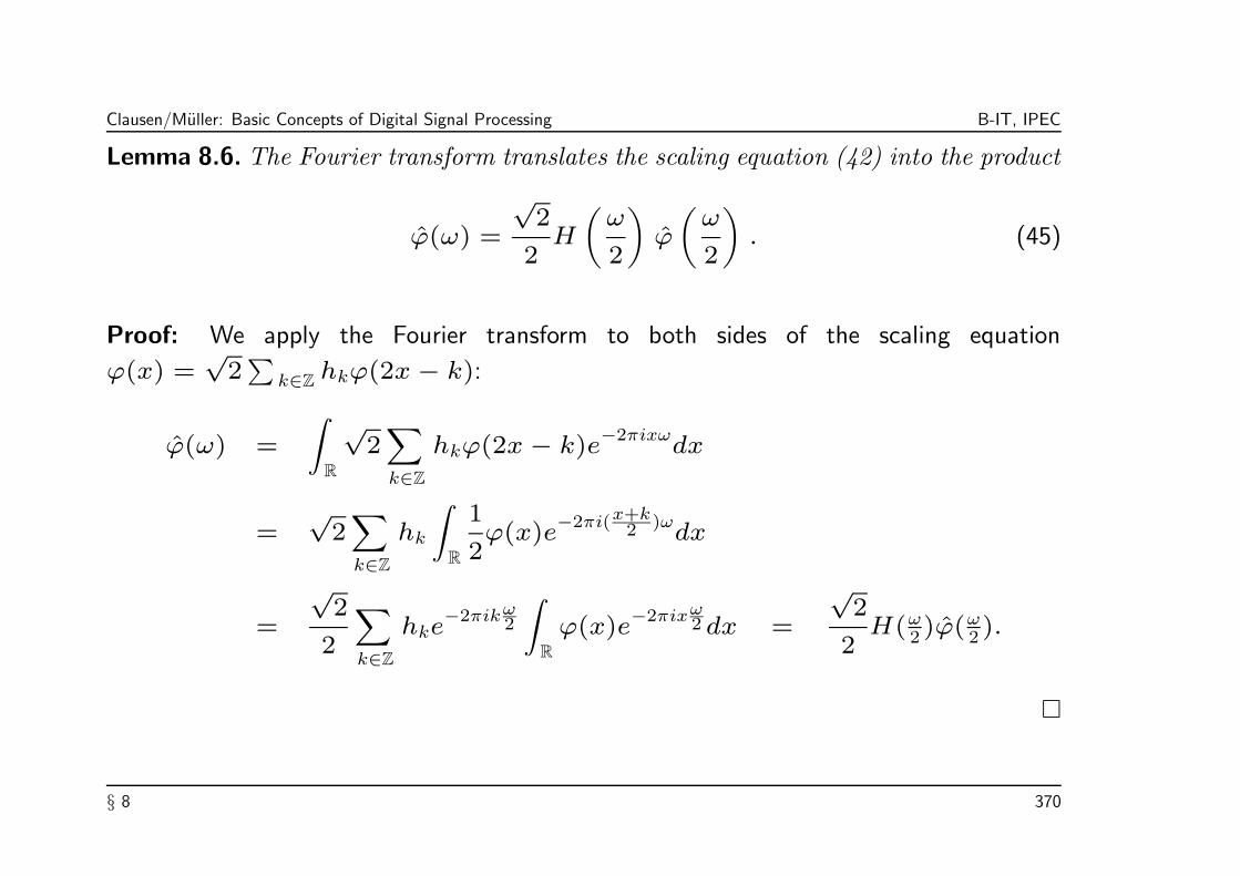
Clausen/Muller: Basic Concepts of Digital Signal Processing B-IT, IPEC
Lemma 8.6. The Fourier transform translates the scaling equation (42) into the product
ϕ(ω) =
√2
2H
(ω
2
)ϕ
(ω
2
). (45)
Proof: We apply the Fourier transform to both sides of the scaling equation
ϕ(x) =√
2∑
k∈Zhkϕ(2x− k):
ϕ(ω) =
∫
R
√2∑
k∈Z
hkϕ(2x− k)e−2πixω
dx
=√
2∑
k∈Z
hk
∫
R
1
2ϕ(x)e
−2πi(x+k2 )ωdx
=
√2
2
∑
k∈Z
hke−2πikω2
∫
R
ϕ(x)e−2πixω2dx =
√2
2H(ω2 )ϕ(ω2).
§ 8 370

Clausen/Muller: Basic Concepts of Digital Signal Processing B-IT, IPEC
The product (45) is easier to deal with when using analytic methods. The frequency
response H exhibits information about the filter properties of the filter h = (hk)k∈Z.
The following theorem gives the mathematical fundament for the interpretation of h.
Theorem 8.7. Let h = (hk)k∈Z be the scaling filter of an MRA. Then the frequency
response H satisfies the so-called orthogonality relation
|H(ω)|2 + |H(ω + 1
2
)|2 = 2. (46)
Furthermore, the frequency response assumes the following values:
H(0) =√
2 and H(
12
)= 0, (47)
which is equivalent to
∑
k∈Z
hk = H(0) =√
2 and∑
k∈Z
(−1)khk = H
(12
)= 0. (48)
Proof: We refer to p. 114 of [Louis/Maaß/Rieder] or to [Burrus/Gopinath/Guo].
§ 8 371

Clausen/Muller: Basic Concepts of Digital Signal Processing B-IT, IPEC
Note 8.8. Using the language of filter design, Theorem 8.7 can be interpreted as follows:
• In the case that the scaling function ϕ is a real-valued function, the scaling filter
h = (hk)k∈Z are real-valued as well.
• Furthermore, assuming h ∈ `1(Z), H defines a (1-periodic) continuous function.
Then, the values of Equation (47) imply that |H| is small in a neighborhood of ω = 12
and |H| ≈ 1 in a neighborhood of ω = 0.
• In other words, the scaling filter h = (hk)k∈Z can be regarded as a low-pass filter.
§ 8 372

Clausen/Muller: Basic Concepts of Digital Signal Processing B-IT, IPEC
To the scaling filter h = (hk)k∈Z we associate the filter g = (gk)k∈Z defined by
gk := (−1)kh1−k. (49)
Then for the frequency response G follows
G(ω) =∑
k∈Z
gke−2πikω
=∑
k∈Z
(−1)kh1−ke
−2πikω
=∑
k∈Z
h1−ke−2πik(ω+1
2)
=∑
k∈Z
hke−2πi(1−k)(ω+1
2)
= e−2πi(ω+1
2)∑
k∈Z
hke−2πik(ω+1
2)
= −e−2πiωH(ω +1
2
).
§ 8 373

Clausen/Muller: Basic Concepts of Digital Signal Processing B-IT, IPEC
From this and Theorem 8.7 we obtain the following result.
Corollary 8.9. The frequency responses G and H bear the following relation:
|H(ω)|2 + |G(ω)|2 = 2. (50)
Furthermore, the frequency response G assumes the values
G(0) = 0, and G(
12
)=
√2. (51)
In other words, the convolution filter defined by g is a high-pass filter.
§ 8 374

Clausen/Muller: Basic Concepts of Digital Signal Processing B-IT, IPEC
8.2.2 Filter Coefficients and Wavelets
The scaling filter coefficients allow us to construct the wavelets as announced in the main
result at the beginning of this section.
Theorem 8.10. Let Vm|m ∈ Z be an MRA with scaling function ϕ ∈ V0. The
function ψ ∈ V−1 defined by
ψ(x) =√
2∑
k∈Z
gkϕ(2x− k) :=∑
k∈Z
gkϕ−1,k(x), (52)
gk := (−1)kh1−k, (53)
where hk|k ∈ Z are the coefficients of the scaling equation (42) has the following
properties:
(i) ψm,k(·) := 2−m/2ψ(2−m · −k)|k ∈ Z is an ONB for Wm.
(ii) ψm,k|m, k ∈ Z is an ONB for L2(R).
(iii) ψ is a wavelet with cψ =∫
R|ω|−1|ψ(ω)|2dω = 2ln2.
§ 8 375

Clausen/Muller: Basic Concepts of Digital Signal Processing B-IT, IPEC
Proof: In the first step we show ψ ∈ W0 ⊂ V−1:
〈ψ(·)|ϕ(· − n)〉 (42)= 2
∑
k∈Z
∑
l∈Z
gkhl〈ϕ(2 · −k)|ϕ(2 · −2n− l)〉
=∑
k∈Z
∑
l∈Z
gkhlδk,2n+l =∑
l∈Z
g2n+lhl
(53)=
∑
l∈Z
(−1)2n+l
h1−(2n+l)hl
=∑
l∈Z
h1−2(n+l)h2l −∑
l∈Z
h−2(n+l)h2l+1
=∑
λ∈Z
h1+2λh−2(λ+n) −∑
l∈Z
h−2(n+l)h2l+1
= 0.
§ 8 376

Clausen/Muller: Basic Concepts of Digital Signal Processing B-IT, IPEC
Using Equation (44), a similar computation verifies the orthonormality of
ψ(· − k)|k ∈ Z.
To complete the proof of (i) and (ii) we have to show the completeness of the system
ψ(· − k)|k ∈ Z
in W0. To this means it is sufficient to show the completeness of the orthonormal system
ϕ(· − k), ψ(· − k)|k ∈ Z
in V−1 since V0 ⊕W0 = V−1. For this part, it is sufficient to show that
ϕ−1,0 =√
2ϕ(2·)
is representable by
ϕ(· − k), ψ(· − k)|k ∈ Z.
§ 8 377

Clausen/Muller: Basic Concepts of Digital Signal Processing B-IT, IPEC
We use Equation (42) and Equation (52) and show that Parseval’s identity holds:
2∑
k∈Z
(|〈ϕ(2·)|ϕ(· − k)〉|2 + |〈ϕ(2·)|ψ(· − k)〉|2
)
= 4∑
k∈Z
(∣∣∣∑
l∈Z
hl〈ϕ(2·)|ϕ(2 · −2k − l)〉∣∣∣2
+∣∣∣∑
l∈Z
gl〈ϕ(2·)|ψ(2 · −2k − l)〉∣∣∣2)
=∑
k∈Z
(∣∣∣∑
l∈Z
hlδ0,2k+l
∣∣∣2
+∣∣∣∑
l∈Z
(−1)lh1−lδ0,2k+l
∣∣∣2)
=∑
k∈Z
h22k +
∑
k∈Z
h22k+1
=∑
k∈Z
h2k
Lemma8.5= 1 = ||ϕ−1,0||2.
The proof of (iii) is more extensive and can be found in [Louis/Maaß/Rieder].
§ 8 378

Clausen/Muller: Basic Concepts of Digital Signal Processing B-IT, IPEC
Lemma 8.11. The translated and dilated versions ψm,k of the wavelet ψ satisfy the
scaling equation:
ψm,k =∑
j∈Z
gjϕm−1,2k+j. (54)
Proof: This follows from the from the scaling equation (52) in the same way as in Lemma
8.4.
The coefficients (hk)k∈Z are denoted as scaling filter coefficients and the coefficients
(gk)k∈Z as wavelet filter coefficients associated to the MRA. We also speak from the
scaling filter h = (hk)k∈Z and wavelet filter g = (gk)k∈Z. For an example of the theory
introduced so far, we refer to Section 8.3 where the Haar-MRA is discussed in detail.
§ 8 379

Clausen/Muller: Basic Concepts of Digital Signal Processing B-IT, IPEC
Note 8.12. The wavelet associated to the MRA is not uniquely determined. However,
if the wavelet ψ is defined by equations (52) and (53), the wavelet is real valued in
case the scaling function ϕ is real valued. This is an important property in view of an
implementation of the wavelet algorithms discussed in the next section. For further details
we refer to p. 117 of [Louis/Maaß/Rieder].
§ 8 380

Clausen/Muller: Basic Concepts of Digital Signal Processing B-IT, IPEC
8.2.3 Fast Wavelet Algorithms
From the interplay of MRA and wavelet theory one can derive the
fast discret wavelet transform, which is the content of this section. It seems to be
an odd consequence that a wavelet transform based on a wavelet associated to some MRA
can be performed without knowing the wavelet explicitly. All we need to know are the
scaling filter coefficients (hk)k∈Z defined by the scaling equation (42).
Instead of computing wavelet coefficients 〈f |ψs,t〉 by computing the integrals of the inner
products, one does smoothing much easier: the signal (or, to be more precise, a discretized
form of the signal) is convolved with the low-pass filter h = (hk)k∈Z (scaling coefficients)
and the associated high-pass filter g = (gk)k∈Z (wavelet filter coefficients). The details
of this procedure will be explained in the next subsections.
§ 8 381

Clausen/Muller: Basic Concepts of Digital Signal Processing B-IT, IPEC
8.2.4 Fast Discrete Wavelet Transform (FDWT)
In this subsection we introduce the algorithm for the fast computation of the discrete
wavelet transform. Based on the underlying MRA the algorithm can be derived from the
scaling equation (42) in an elegant fashion.
We fix an MRA with scaling function ϕ and start with a signal f which lies in the
base space V0 of the MRA. As it turns out, this assumption on f will be the actual
discretization step (see subsection 8.2.7). By Definition 8.1, the signal f can be written as
f(x) =∑
k∈Z
v0kϕ(x− k) (55)
with a suitable family of coefficients
v0= (v
0k)k∈Z.
§ 8 382

Clausen/Muller: Basic Concepts of Digital Signal Processing B-IT, IPEC
As before, let ψ denote the orthonormal wavelet associated to ϕ (see (52)). Then
ψm,k = 2−m/2
ψ(2−m · −k)|m, k ∈ Z
defines an ON basis of L2(R). The goal is to compute the wavelet coefficients
f(2m, 2
mk) = 〈f |ψm,k〉,m ∈ Z, k ∈ Z. (56)
Note that this amounts to evaluating the CWT f on a CWT-adapted discrete-time grid
with a = 2 and b = 1 (see Subsection 7.5.1). The corresponding wavelet frame is an
ON-basis (see Subsection 7.5.2).
§ 8 383

Clausen/Muller: Basic Concepts of Digital Signal Processing B-IT, IPEC
Since f ∈ V0 and L2(R) = V0 ⊕⊕
j≤0Wj by equation (39), it follows immediately
that
〈f |ψm,k〉 = 0 for m ≤ 0, k ∈ Z
Therefore, it suffices to compute f(2m, 2mk) for m ∈ N, k ∈ Z. We introduce the
following notation:
wmk := 〈f |ψm,k〉, w
m= (w
mk |k ∈ Z) ∈ `
2(Z),
vmk := 〈f |ϕm,k〉, v
m= (v
mk |k ∈ Z) ∈ `
2(Z).
§ 8 384

Clausen/Muller: Basic Concepts of Digital Signal Processing B-IT, IPEC
Using the wavelet equation (54) and scaling equation (43) we obtain
wmk = 〈f |ψm,k〉 =
∑
l∈Z
gl〈f |ϕm−1,2k+l〉 =∑
l∈Z
gl−2kvm−1l , (57)
vmk = 〈f |ϕm,k〉 =
∑
l∈Z
hl〈f |ϕm−1,2k+l〉 =∑
l∈Z
hl−2kvm−1l . (58)
These recursive formulas constitute already the wavelet decomposition algorithm: starting
with the sequence v0 we can recursively compute the wavelet coefficients wm, m ∈ N,
from vm−1 which in turn can be recursively computed. Once v0 is known, all operations
are performed on the vm and wm and the signal f is not used any longer. As mentioned
before, the assumption f ∈ V0 is the actual discretization step of the time-continuous
signal f . In Subsection 8.2.7 we will discuss the problems which arise from this assumption
in practice.
§ 8 385

Clausen/Muller: Basic Concepts of Digital Signal Processing B-IT, IPEC
We further investigate the computations in (57) and (58) which will be expressed by the
decomposition operators H and G, respectively. We define
H : `2(Z) → `
2(Z)
v 7→((Hv)k =
∑
l∈Z
hl−2kvl)k∈Z
(59)
and
G : `2(Z) → `
2(Z)
v 7→((Gv)k =
∑
l∈Z
gl−2kvl)k∈Z. (60)
§ 8 386

Clausen/Muller: Basic Concepts of Digital Signal Processing B-IT, IPEC
The operators H and G have a nice interpretation in terms of filter theory: define the
filters h = (h(k))k∈Z) and g = (g(k))k∈Z) by
h(k) = h−k and g(k) = g−k, k ∈ Z,
then H and G are nothing else than convolution with h and g, respectively, and
downsampling by a factor of 2. In other words,
wm
= (↓2)[g ∗ vm−1],
vm
= (↓2)[h ∗ vm−1].
The algorithm for the discrete wavelet transform performed on the first M scales can be
summarized as follows.
§ 8 387
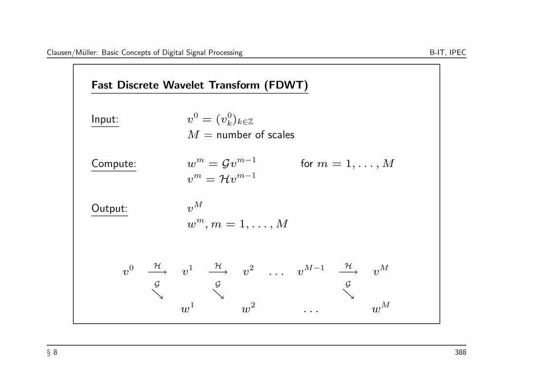
Clausen/Muller: Basic Concepts of Digital Signal Processing B-IT, IPEC
Fast Discrete Wavelet Transform (FDWT)
Input: v0 = (v0k)k∈Z
M = number of scales
Compute: wm = Gvm−1
vm = Hvm−1
for m = 1, . . . ,M
Output: vM
wm,m = 1, . . . ,M
v0 H−→ v1 H−→ v2 . . . vM−1 H−→ vM
G
G
G
w1 w2 . . . wM
§ 8 388

Clausen/Muller: Basic Concepts of Digital Signal Processing B-IT, IPEC
Note 8.13. The algorithm starts with a signal f corresponding to some fine scale (here
f ∈ V0 corresponding to scale 0) and then proceeds in direction of coarser scales. The
choice of V0 as start of the algorithm is arbitrary. One could, as well, start with the space
V−1254 and proceed in the same way.
§ 8 389

Clausen/Muller: Basic Concepts of Digital Signal Processing B-IT, IPEC
8.2.5 Fast Discrete Wavelet Reconstruction (FIDWT)
We now investigate how to reconstruct the sequence v0 and hence the original signal
f ∈ V0,
f(x) =∑
k∈Z
v0kϕ(x− k)
from the sequences of coefficients
vM , wm|m = 1, . . . ,M.
This amounts to the inverse of the discrete wavelet transfrom discussed in the previous
subsection. The corresponding fast algorithm is called fast discrete wavelet reconstruction
or fast inverse discrete wavelet transform (FIDWT).
§ 8 390

Clausen/Muller: Basic Concepts of Digital Signal Processing B-IT, IPEC
We first investigate how to reconstruct the sequence v0 from v1 and w1. Recall that the
space V0 is the orthogonal sum of the subspaces V1 and W1. Therefore
∑
k∈Z
v0kϕ0,k =
∑
j∈Z
v1jϕ1,j +
∑
j∈Z
w1jψ1,j
=∑
j∈Z
v1j
∑
l∈Z
hlϕ0,2j+l +∑
j∈Z
w1j
∑
l∈Z
glϕ0,2j+l,
where we have used the scaling equation (43) and wavelet equation (54). Comparing
coefficients results in
v0k =
∑
j∈Z
v1jhk−2j +
∑
j∈Z
w1jgk−2j. (61)
In the same way, one can reconstruct the sequence vM−1 from wM and vM , M ∈ N.
Proceeding recursively, one can reconstruct v0 from vM and the sequences of wavelet
coefficients wm of the scales m = M,M − 1, . . . , 1.
§ 8 391

Clausen/Muller: Basic Concepts of Digital Signal Processing B-IT, IPEC
This reconstruction algorithm can be expressed by the operators H∗ and G∗ defined by
H∗: `
2(Z) → `
2(Z)
v 7→ ((H∗v)k =
∑
j∈Z
hk−2jvj|k ∈ Z), (62)
G∗: `
2(Z) → `
2(Z)
w 7→ ((G∗w)k =
∑
j∈Z
gk−2jwj|k ∈ Z). (63)
It is not difficult to show that H∗ and G∗ are the adjoint operators to the decomposition
operators H and G of the last subsection, i.e.,
〈Hv|w〉 = 〈v|H∗w〉 and 〈Gv|w〉 = 〈v|G∗
w〉, v, w ∈ `2(Z).
§ 8 392

Clausen/Muller: Basic Concepts of Digital Signal Processing B-IT, IPEC
A single reconstruction step from scale m to m− 1 is described by
vm−1
= H∗vm
+ G∗wm. (64)
As for H and G, the operators H∗ and G∗ also have a nice interpretation in terms of filter
theory: H∗ and G∗ are nothing else then upsampling by a factor of 2 and subsequent
convolution with h and g, respectively. In other words,
vm−1
= h ∗ ((↑2)[vm]) + g ∗ ((↑2)[wm]). (65)
The algorithm for the discrete inverse wavelet transform (FIDWT) starting at scale M
and proceeding up to scale 0 can be summarized as follows.
§ 8 393

Clausen/Muller: Basic Concepts of Digital Signal Processing B-IT, IPEC
Fast Discrete Wavelet Reconstruction (FIDWT)
Input: M = number of scales
vM
wm, m = 1, . . . ,M
Compute: vm−1 = H∗vm + G∗wm for m = M, . . . , 1
Output: v0
vMH∗−→ vM−1 H∗
−→ vM−2 . . . v1 H∗−→ v0
G∗
G∗
G∗
wM wM−1 . . . w1
§ 8 394

Clausen/Muller: Basic Concepts of Digital Signal Processing B-IT, IPEC
Note 8.14. The reconstruction algorithm starts with some sequence vM which corresponds
to some coarse representation of the original signal f . Using successively the wavelet
coefficients wm of the scales m = M,M − 1, . . . 1, the sequences vm are reconstructed
which correspond to finer versions of f for decreasing m. Reaching the scale m = 0 one
has finally reconstructed the original signal f ∈ V0.
§ 8 395

Clausen/Muller: Basic Concepts of Digital Signal Processing B-IT, IPEC
8.2.6 Complexity of the FDWT and FIDWT
We now want to determine the complexity of the algorithms for discrete wavelet transform
and its inverse.
Recall that `(x) denotes the length of a finite DT-signal x ∈ CZ (see Definition 3.23).
We suppose that the length of the input sequence v0 = (v0k)k∈Z has finite length
N := `(v0).
Furthermore, we only consider the case of finite filters h = (hk)k∈Z and g = (gk)k∈Z.
One can show that this holds for any wavelets with compact support such as for the Haar
wavelet or the Daubechies wavelets.
§ 8 396

Clausen/Muller: Basic Concepts of Digital Signal Processing B-IT, IPEC
By definition of g (see (53) of Theorem 8.10) we have `(g) = `(h). In the discrete
wavelet decomposition the coefficient sequences
wm
= Gvm−1und v
m= Hvm−1
are successively computed for m = 1, . . . ,M . The operators H and G can be expressed
as convolution with suitable filters of length `(h) and subsequent 2-downsampling.
By Lemma 3.24 the length of the convolution of two finite sequences x and y is given by
the formula
`(x ∗ y) = `(x) + `(y) − 1.
By 2-downsampling, the length of the resulting sequence is about half the length.
§ 8 397

Clausen/Muller: Basic Concepts of Digital Signal Processing B-IT, IPEC
Therefore, we get for m = 1, . . . ,M
`(vm) ≤ d1
2(`(vm−1) + `(h) − 1)e ≤ 1
2(`(vm−1) + `(h))
`(wm) ≤ d1
2(`(vm−1) + `(g) − 1)e ≤ 1
2(`(vm−1) + `(h))
From this, we inductively get the estimates
`(vm) ≤ 2
−m`(v
0) + `(h), (66)
`(wm) ≤ 2
−m`(v
0) + `(h). (67)
Furthermore, note that the algorithm terminates if M ≥ log2N . In other words, the
number M of scales, which have to be computed, is bounded by log2N .
§ 8 398

Clausen/Muller: Basic Concepts of Digital Signal Processing B-IT, IPEC
Using a straightforward algorithm to compute the convolution x ∗ y of two finite signals x
and y (note that there are in general more efficient algorithms) takes at most 2`(x)`(y)
operations (additions and multiplications). Therefore, the overall cost OC for computing
the sequences vm and wm for the scales m = 1, . . . ,M is bounded by
OC ≤M∑
m=1
(2`(vm)`(h) + 2`(w
m)`(g))
≤M∑
m=1
4(2−m`(v
0)`(h) + `(h)
2)
≤ 4`(v0)`(h) + 4M`(h)
2.
Since M is bounded by log2N we get the result as summarized in the next theorem.
§ 8 399

Clausen/Muller: Basic Concepts of Digital Signal Processing B-IT, IPEC
Theorem 8.15. Let V0 be the base space of an MRA with scaling function ϕ, associated
wavelet ψ and filter coefficients h = (hk)k∈Z of finite length `(h). Furthermore, let
f ∈ V0 be a signal with f(x) =∑
k∈Zv0kϕ(x− k) such that the coefficient sequence
v0 = (v0k)k∈Z is of finite length N = `(v0). Then the overall complexity OC to
compute the discrete wavelet transform f with respect to the mother wavelet ψ is
OC = O(N).
To be more explicit, one has the bound OC ≤ c`(h)N , where c`(h) is a constant which
depends linearly on the filter length `(h).
The overall complexity of the inverse transform (FIDWT) can be determined in a similar
fashion and results in a complexity of the same order as in Theorem 8.15.
§ 8 400
Clausen/Muller: Basic Concepts of Digital Signal Processing B-IT, IPEC
8.2.7 Discretization step in the DWT
Again, we want to emphasize that in the fast discrete wavelet transform neither the
analyzing wavelets ψs,t nor the analyzed signal f are discrete. Discrete is only the grid on
which the wavelet coefficients wmk = 〈f |ψm,k〉 are computed given by the integrals
〈f |ψm,k〉 =
∫
R
f(u)ψm,k(u)du.
Also these integrals are computed precisely by the FDWT and not approximately, as one
might guess. However, the integrals are not computed directly but recursively using the
values of integrals corresponding to lower scales.
§ 8 401

Clausen/Muller: Basic Concepts of Digital Signal Processing B-IT, IPEC
These facts are surprising at first sight and the following kind of questions come into mind:
• How is it possible to compute integrals of time-continuous functions by some discrete
algorithm?
• Where lies the actual discretization step which connects the CT-world (the signal f
and the wavelets ψm,k) with the DT-world?
The answer to these questions lies in the assumption (55) that the signal f lies in the base
space V0 of the MRA. In other words, in order for the FDWT algorithm to get started
ones needs the assumption that f can be developed as
f(x) =∑
k∈Z
v0kϕ(x− k)
with a family of coefficients
v0= (v
0k = 〈f |ϕ(· − k)〉)k∈Z.
§ 8 402

Clausen/Muller: Basic Concepts of Digital Signal Processing B-IT, IPEC
The coefficient sequence v0 is the starting point for the recursive FDWT. In theory, this
algorithm is very elegant when having the “right” assumptions. In practice, however, there
are quite some open problems:
• How does one obtain from the original CT-signal f ∈ L2(R) a signal in the base
space V0, which is needed as starting point for the recursive FDWT?
• The assumption f ∈ V0 guarantees the existence of a coefficient sequence
v0 = (v0k)k∈Z. However, how can the coefficients v0
k = 〈f |ϕ(· − k)〉, which are
given by integrals, be computed in practice? Even computing the integrals numerically
(for example, approximation by Riemann sums) is in general very expensive and
inefficient.
• In digital signal processing the signals are in general not given as CT-signals f ∈ L2(R)
but as sampled DT-signals (f(k))k∈Z. How can the FDWT used for such DT-signals?
§ 8 403

Clausen/Muller: Basic Concepts of Digital Signal Processing B-IT, IPEC
In practice there is an easy “solution” to all of these problems: just use the samples
(f(k))k∈Z of the CT-signal f as coefficient sequence (v0k)k∈Z. Strictly speaking, this
identification does in general not make sense. In the following we cite Strang und Nguyen
who write in their book [Strang/Nguyen]:
... Is this legal [to use the samples f(k) instead of the coefficients (v0k)]? No. It is a
wavelet crime. Some can’t imagine doing it, others can’t imagine not doing it. Is this
crime convenient? Yes. We may not know the whole function t 7→ f(t), it may not
be a combination of (ϕ(· − k)k∈Z, and computing the true coefficients (v0k)k∈Z may
take too long. But the crime cannot go unnoticed - we have to discuss it.
§ 8 404

Clausen/Muller: Basic Concepts of Digital Signal Processing B-IT, IPEC
For a detailed discussion we refer to p. 232 of [Strang/Nguyen]. We restrict ourselves to
some remarks. The basic assumption when identifying samples with coefficients is
v0k ≈ f(k), for k ∈ Z.
Actually, this is true for many scaling functions ϕ which behave like the Dirac function δ.
In other words, if ϕ is concentrated around the point of time t = 0 like a peak and its
integral is 1 then 〈f |ϕ〉 ≈ 〈f |δ〉. Then, the same holds for the corresponding translates
of ϕ and δ and we get
v0k = 〈f |ϕ(· − k)〉 ≈ 〈f |δ(· − k)〉 = f(k).
Therefore, in practice it is important to check if this approximation property is actually
satisfied — depending on the underlying MRA and its associated wavelet and the signal f .
§ 8 405

Clausen/Muller: Basic Concepts of Digital Signal Processing B-IT, IPEC
If the approximation property does not hold, the samples values have to be suitably
preprocessed using so-called prefilters. These modified samples can then be used as
starting coefficients in the FDWT instead of the (v0k)k∈Z.
Conclusion: If for a given MRA and a signal f one has v0k ≈ f(k), the samples (fk)k∈Z
(possibly preprocessed ) can be used instead of the coefficients (v0k)k∈Z as starting values
for the FDWT. In this case, however, the wavelet coefficients wmk are faulty, even though
the FDWT computes exactly. The quality of the wmk depends solely on the approximation
quality of the input data.
§ 8 406

Clausen/Muller: Basic Concepts of Digital Signal Processing B-IT, IPEC
8.2.8 Pm, Qm and Wavelet Coefficients
The FDWT computes from the input sequence of scaling coefficients v0 = (v0k)k∈Z of
some signal f ∈ V0 the sequence of wavelet coefficients wm = (wmk )k∈Z for the scales
m = 1, . . . ,M and the sequence of scaling coefficients vM = (vMk )k∈Z on scale M .
With these data the projections Qm of f on Wm are given by
Qm(f) =∑
k∈Z
〈f |ψm,k〉ψm,k =∑
k∈Z
wmk ψm,k,
m = 1, . . . ,M , and the projection PM of f on VM is given by
PM(f) =∑
k∈Z
〈f |ϕM,k〉ϕM,k =∑
k∈Z
vMk ϕM,k.
Similarly, the projections Pm(f) can be computed by using the scaling coefficients vm for
the scales m = M, . . . , 1, wich in turn can be computed by the FIDWT.
§ 8 407

Clausen/Muller: Basic Concepts of Digital Signal Processing B-IT, IPEC
Since in practice neither the scaling function ϕ nor the mother wavelet ψ are known
explicitly, the projections can not very well be computed even though the wavelet and
scaling coefficients are known. Many “wavelet specialists” read the properties of some
signal f directly from the wavelet coefficients. For a graphical representation of the
wavelet coefficients (if there are only a finite number, i.e., if the sequence v0 has finite
length N) one constructs one sequence
w(f) := (vM, w
M, w
M−1, . . . , w
1) (68)
from the M + 1 sequences w1, . . . , wM and vM . This representation is, for example,
used in Figure 40 of Chapter 9.
§ 8 408

Clausen/Muller: Basic Concepts of Digital Signal Processing B-IT, IPEC
In concrete applications the length N = `(v0) of the input sequence, which also
determines the complexity of the FDWT and FIDWT, is much larger then the filter lengths
`(h) = `(g). For example, one has often N > 104, whereas `(h) ≤ 8. Therefore, from
the estimations (66) and (67) follows
`(w(f)) ≈ N.
If one considers signals f ∈ V0 with `(v0) = N ∈ N, where N is a power of two, one
can achieve by a small modification of the FDWT that the output sequence w(f) as given
in Equation (68) has also length N . The so modified FDWT mapping the N coefficients
of v0 to the N coefficients of w(f) can be realized by an orthonormal N × N -matrix.
For details we refer to [Strang/Nguyen].
§ 8 409

Clausen/Muller: Basic Concepts of Digital Signal Processing B-IT, IPEC
Warning: Finally, we repeat one of our warnings concerning the L2 norm. We have seen
that any signal f ∈ L2(R) can be represented as
f =∑
m∈Z
∑
k∈Z
〈f |ψm,k〉ψm,k.
This equation holds again only in the L2-sense! It is important to be conscious of this
fact since otherwise paradoxical implications arise. In the following we give an example.
For each n ∈ N we define
fn :=∑
−n≤m≤n
∑
−n≤k≤n〈f |ψm,k〉ψm,k.
§ 8 410

Clausen/Muller: Basic Concepts of Digital Signal Processing B-IT, IPEC
Since for all wavelets ψm,k,m, k ∈ Z, the mean value
∫
R
ψm,k(t)dt
is zero, the same holds for each function fn. Since f is the limit function of fn for
n → ∞, one could think that the mean value of f also has to be zero even though this
does not hold for a general function f ∈ L2(R).
Here the fact is decisive that the sequence (fn)n∈N does not converge in the L1-norm (in
this case the mean value of f would have to vanish) but converges in the L2-norm. In
other words, it is possible to represent an arbitrary function in f ∈ L2(R) as an L2-limit
of functions whose mean value is zero.
§ 8 411

Clausen/Muller: Basic Concepts of Digital Signal Processing B-IT, IPEC
8.3 Example: Haar-MRA
In this section, we illustrate the theory introduced before by means of the Haar-MRA as
an example. Already in 1910, Haar showed that certain translated and scaled version of
the box function form a basis of L2(R). In much later years, it was discovered that this
system — also referred to as Haar system — constitutes the easiest example for an MRA.
§ 8 412
Clausen/Muller: Basic Concepts of Digital Signal Processing B-IT, IPEC
Let V0 be the space of functions in L2(R), which are constant on all intervals
[k, k + 1[, k ∈ N.
Any function f ∈ V0 is determined by its values f(k) at the points of time t = k.
k ∈ N. Note that the function t 7→ f(2t) ist constant at all intervals of the form
[k/2, (k + 1)/2[ for k ∈ N.
The space of all such functions is denoted by V−1. In a similar fashion, we define the
space Vm,m ∈ Z, as space of functions being constant on the so-called dyadic intervals
of length 2m. Here, a dyadic interval of length 2m is defined by
Im,k := [k · 2m, (k + 1) · 2m[ for k ∈ N.
§ 8 413
Clausen/Muller: Basic Concepts of Digital Signal Processing B-IT, IPEC
Obviously, one has the inclusions
0 ⊂ . . . ⊂ V2 ⊂ V1 ⊂ V0 ⊂ V−1 ⊂ V−2 ⊂ . . . ⊂ L2(R),
since each function being constant at the intervals of length 2−m are, of course, also
constant on the intervals of half the length. The properties
⋂
m∈Z
Vm = 0 and f(·) ∈ Vm ⇐⇒ f(2m·) ∈ V0
are also easy to see. The actual achievement of Haar was to show that
⋃
m∈Z
Vm = L2(R).
In other words, the L2-step functions on the dyadic intervals are dense in L2(R), i.e.,
each function in L2(R) can be approximated by such step functions (in the L2 sense).
For a proof of this fact, we have to refer to the literature.
§ 8 414

Clausen/Muller: Basic Concepts of Digital Signal Processing B-IT, IPEC
Up to the existence of a scaling function, we have seen that the spaces Vm, m ∈ Z,
satisfy the axioms of an MRA (see Definition 8.1). Define
ϕ(t) :=
1 if 0 ≤ t < 1
0 otherwise,
which is also illustrated in Figure 32. The box function ϕ is obviously orthogonal to
its integral translates t 7→ ϕ(t − k), k ∈ Z, and these translates form an ONB of V0.
Therefore, ϕ defines a scaling function as postulated and makes Vm, m ∈ Z, to an MRA
which is also denoted as Haar-MRA.
§ 8 415

Clausen/Muller: Basic Concepts of Digital Signal Processing B-IT, IPEC
For the Haar-MRA we summarize the results which were derived for general MRAs in the
last section. The existence of a scaling equation ist guaranteed by Lemma 8.2. In our
example, one can easily guess the scaling coefficients. One has
h0 =1√2, h1 =
1√2, (69)
and all other coefficients are zero. This filter was, up to a factor, already investigated in
Subsection 3.6.1. Recall that the frequency response H of h := (hk)k∈Z is given by
H(ω) =1√2
+1√2e−2πiω
= e−πiω√
2 cos(πω).
As was shown in Theorem 8.7, one indeed has H(0) =√
2 and H(12) = 0.
§ 8 416

Clausen/Muller: Basic Concepts of Digital Signal Processing B-IT, IPEC
The scaling filter coefficients h = (hk)k∈Z define a lowpass filter. The associated wavelet
filter coefficients g = (gk)k∈Z are given by
g0 = h1 =1√2, g1 = (−1)h0 = − 1√
2, (70)
and all other coefficients are zero. The mother wavelet of the MRA is by Theorem 8.10
defined by
ψ(x) =√
2∑
k∈Z
gkϕ(2x− k)
=
1 if 0 ≤ t < 12
−1 if 12 ≤ t < 1
0 otherwise.
§ 8 417
Clausen/Muller: Basic Concepts of Digital Signal Processing B-IT, IPEC
This is the so-called Haar wavelet, which we already encountered in Figure 19. We
already know from Theorem 7.4 that the Haar wavelet is indeed a wavelet in the sense of
Definition 7.1. This follows now again from Theorem 8.10. Furthermore, the
ψm,k|k ∈ Z, k ∈ Z,
form an ONB of Wm and
ψm,k|m, k ∈ Z,
from an ONB of L2(R). Among others, it follows that the mother wavelet ψ ∈ W0 is
orthogonal to the scaling function ϕ ∈ V0 and its translates.
Figure 32 shows the Haar scaling function ϕ, the corresponding Haar wavelet ψ, and the
frequency responses of the scaling and wavelet filter coefficients.
§ 8 418

Clausen/Muller: Basic Concepts of Digital Signal Processing B-IT, IPEC
−0.5 0 0.5 1 1.5
−1
−0.5
0
0.5
1
Time t
Scaling function
−0.5 0 0.5 1 1.5
−1
−0.5
0
0.5
1
Time t
Haar wavelet ψ
0 0.2 0.4 0.6 0.8 10
0.5
1
1.5
Frequency ω
Magnitude response |H|
0 0.2 0.4 0.6 0.8 10
0.5
1
1.5
Frequency ω
Magnitude response |G|
Figure 32: Haar-MRA.
§ 8 419

Clausen/Muller: Basic Concepts of Digital Signal Processing B-IT, IPEC
We now want to perform the FDWT from Subsection 8.2.4 w.r.t. the Haar wavelet ψ on
some concrete input signal. The signal f ∈ V0 shown in Figure 33 is given by
f(t) = 1 · ϕ(t) + 1 · ϕ(t− 1) + (−1) · ϕ(t− 2) + (−1) · ϕ(t− 3)
+(−1) · ϕ(t− 4) + (−1) · ϕ(t− 5) + (−2) · ϕ(t− 6) + 2 · ϕ(t− 7).
Using the notation of Subsection 8.2.4, the input coefficient sequence v0 = (v0k)k∈Z for
the FDWT is given by is given by
v0= (1, 1,−1,−1,−1,−1,−2, 2).
(All other coefficients are zero and we only write in the following the above coefficients.)
§ 8 420

Clausen/Muller: Basic Concepts of Digital Signal Processing B-IT, IPEC
Using the filters h and g (see (69) and (70)) we recursively compute the sequences vm of
scaling coefficients for m = 1, . . . ,M by the formula
vmk =
∑
l∈Z
hl−2kvm−1l =
1√2vm−12k +
1√2vm−12k+1
and the sequence wm of wavelet coefficients by
wmk =
∑
l∈Z
gl−2kvm−1l =
1√2vm−12k − 1√
2vm−12k+1.
§ 8 421

Clausen/Muller: Basic Concepts of Digital Signal Processing B-IT, IPEC
Using these formulas, the FDWT proceeds as follows:
v0 1 1 −1 −1 −1 −1 −2 2
v1 √2 −
√2 −
√2 0
w1 0 0 0 −2√
2
v2 0 −1
w2 2 −1
v3 −1√2
w3 1√2
Figure 33 shows the signal f and its projections Pi(f) and Qi(f) onto the subspaces Viand Wi, respectively, for i = 1, 2, 3. The projection Q2(f), for example, is computed
from w2 by
Q2(f) =∑
k∈Z
w2kψ2,k = 2ψ2,0 − 1ψ2,1 = ψ
( ·4
)− 1
2ψ
(· − 4
4
).
§ 8 422

Clausen/Muller: Basic Concepts of Digital Signal Processing B-IT, IPEC
0 2 4 6 8
−2
0
2
f
Signal f and DWT w.r.t the Haar wavelet on the first three scales
0 2 4 6 8
−2
0
2
f
0 2 4 6 8
−2
0
2
P1(f)
0 2 4 6 8
−2
0
2
Q1(f)
0 2 4 6 8
−2
0
2
P2(f)
0 2 4 6 8
−2
0
2
Q2(f)
0 2 4 6 8
−2
0
2
P3(f)
Approximations of f0 2 4 6 8
−2
0
2
Q3(f)
Details of f
Figure 33: Example of a DWT w.r.t. the Haar wavelet of the signal f
§ 8 423

Clausen/Muller: Basic Concepts of Digital Signal Processing B-IT, IPEC
Finally, we want to look at the DWT w.r.t. the Haar wavelet of two signals we have
already encountered in several examples.
Figure 34 shows the projections of the chirp signal
f(t) = sin(20π(t/N)2)
onto the spaces Vi and Wi for the scales i = 1, 2 . . . ,M , M = 7. To this means we
have sampled f at the points t = 1, 2, . . . , N , N = 128, and the sequence of samples
was taken as sequence v0 of scaling coefficients based on the assumption
v0k−1 ≈ f(k) fur k = 1, 2, . . . , N.
We recall that this identification can lead to faulty and meaningless wavelet coefficients
in case the above approximation assumption does not hold. For a discussion we refer to
Section 8.2.7.
§ 8 424

Clausen/Muller: Basic Concepts of Digital Signal Processing B-IT, IPEC
−1
0
1
f
Chirp function f(t)=sin(20π (t/N)2), N=128, and DWT w.r.t the Haar wavelet on the first 7 scales
−1
0
1
f
−1
0
1P
1(f)
−1
0
1Q
1(f)
−1
0
1P
2(f)
−1
0
1Q
2(f)
−1
0
1P
3(f)
−1
0
1Q
3(f)
−1
0
1P
4(f)
−1
0
1Q
4(f)
−1
0
1P
5(f)
−1
0
1Q
5(f)
−1
0
1P
6(f)
−1
0
1Q
6(f)
0 50 100−1
0
1P
7(f)
Approximations of f0 50 100
−1
0
1Q
7(f)
Details of f
Figure 34: Haar-DWT of some chirp signals
§ 8 425

Clausen/Muller: Basic Concepts of Digital Signal Processing B-IT, IPEC
Figure 34 illustrated very well the following principles.
• The wavelet coefficients of scales with small index encode the high-frequency
components of the signal f .
• On the first scale the “details” Q1(f) increase in time which corresponds to the
increasing frequency of the chirp signal f .
• The projection P1(f) is the difference of the signals f and the detail Q1(f).
• Computing the second scale, the projection P1(f) is further decomposed into a
high-frequency component, the detail Q2(f), and a low-frequency component P2(f).
P2(f) is a smoothed version of P1(f).
• This procedure is now iterated up to projections P7(f) which is a constant function
on [1 : N ]. This is the case, when in the DFT there is only one non-trivial coefficient
left in the sequence vM (here M = 7).
§ 8 426
Clausen/Muller: Basic Concepts of Digital Signal Processing B-IT, IPEC
Similarly, Figure 35 shows a signal f which is the superposition of two sines of frequencies
ω = 50 and ω = 5, respectively, with two impulses at t = N/4 and t = N/2,
N = 128. The interpretation of the projections Pi(f) and Qi(f) for i = 1, 2 . . . ,M ,
M = 7, is as in the last example. The impulses can be very well identified in the
high-frequency details Q1(f) und Q2(f). The sine of frequency ω = 50 is represented
mainly in detail Q2(f), whereas the sine of frequency ω = 5 is mainly reflected by the
projections P2(f) and P3(f).
§ 8 427

Clausen/Muller: Basic Concepts of Digital Signal Processing B-IT, IPEC
−4−2
024
f
f(t)=sin(100π (t/N))+sin(10π (t/N)), N=256, impulses at t=64 and t=128, and DWT w.r.t the Haar wavelet, 5 scales
−4−2
024
f
−4−2
024
P1(f)
−4−2
024
Q1(f)
−4−2
024
P2(f)
−4−2
024
Q2(f)
−4−2
024
P3(f)
−4−2
024
Q3(f)
−4−2
024
P4(f)
−4−2
024
Q4(f)
0 50 100 150 200 250−4−2
024
P5(f)
Approximations of f0 50 100 150 200 250
−4−2
024
Q5(f)
Details of f
Figure 35: Haar-DWT of the superposition of two sines with two impulses
§ 8 428

Clausen/Muller: Basic Concepts of Digital Signal Processing B-IT, IPEC
Chapter 9: DWT-Based Applications
In the previous chapters we have studied various transforms of a signal f such as the
Fourier transform, the WFT and the DWT. The signal f gives, for example, information
about the amplitude of some waveform at a given point in time or the pixel value of
some picture at a given point in space. The goal of the transforms is to exhibit other
information about the signal such as the frequency content of the signal or the occurrences
of certain singularities (e.g., in higher derivatives of f which cannot be seen in the
time-representation). The transforms provide a different representation of the signal, one
also often speaks of transformation domain, in which properties of f can be read off which
can not be seen in the time domain.
For example, from the Fourier transform of f or from the Fourier domain one can read
off the spectral content of f . Or in the DWT domain, i.e., from the wavelet coefficients,
one can determine which details (scale parameter s) occur in f at a given time (time
parameter t) in which intensity (size of wavelet coefficient).
§ 9 429
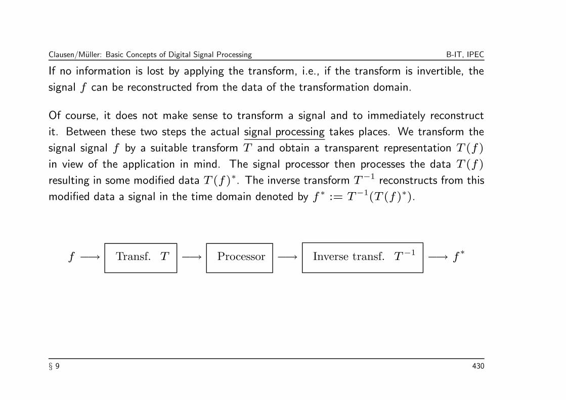
Clausen/Muller: Basic Concepts of Digital Signal Processing B-IT, IPEC
If no information is lost by applying the transform, i.e., if the transform is invertible, the
signal f can be reconstructed from the data of the transformation domain.
Of course, it does not make sense to transform a signal and to immediately reconstruct
it. Between these two steps the actual signal processing takes places. We transform the
signal signal f by a suitable transform T and obtain a transparent representation T (f)
in view of the application in mind. The signal processor then processes the data T (f)
resulting in some modified data T (f)∗. The inverse transform T−1 reconstructs from this
modified data a signal in the time domain denoted by f ∗ := T−1(T (f)∗).
f −→ Transf. T −→ Processor −→ Inverse transf. T−1 −→ f∗
§ 9 430

Clausen/Muller: Basic Concepts of Digital Signal Processing B-IT, IPEC
All transforms T we have considered so far are continuous operators with continuous
inverse operator T−1. This property is important in signal processing since small
modifications of the data T (f) also result only in small deviations of the original signal
when transformed back into the time domain.
In this chapter we discuss some DWT-based applications. Important is the property of
the wavelet transform that for a large class of relevant signals the energy of a signal is
concentrated in few wavelet coefficients when transformed to the DWT domain. This
property can be exploited to develop methods to represent a signal in a compressed form.
For example, the FBI uses DWT-based compression methods to store finger prints in a
digital library.
§ 9 431

Clausen/Muller: Basic Concepts of Digital Signal Processing B-IT, IPEC
Furthermore, the property of the DWT that the essential properties of a signal are reflected
by only few, but large wavelet coefficients can be used to detect noise in a signal and to
possibly separate it from the signal. DWT-based denoising methods have been successively
applied to examine a recording played by Brahms in 1889 of one of his own compositions
(a version of the Hungarian Dance No. 1). In 1935 an LP disc was directly cut from the
original wax cylinder recording. However, the quality of this record was so poor — the
actual interpretation was submerged into noise — that the recording was more or less
useless for musicological examinations. Using DWT-based methods it was possible for
the first time to extract musicologically relevant information, which exhibited interesting
information about the way how Brahms interpreted one of his own pieces. For example,
one found out that Brahms took the liberty to considerably deviate from the score and
extemporize freely (see [Hubbard] for more details).
§ 9 432

Clausen/Muller: Basic Concepts of Digital Signal Processing B-IT, IPEC
9.1 DWT-Based Denoising
The main of idea of DWT-based denoising can be summarized as follows:
(1) The noisy signal f is transformed by a suitable DWT.
(2) In the transformation domain, T (f) is processed by some thresholding method, i.e.,
wavelet coefficients are removed which lie beyond some suitably chosen thresholds.
This results in the data T (f)∗.
(3) The reconstruction by means of the inverse DWT from the modified wavelet
coefficients T (f)∗ gives the denoised signal f ∗.
§ 9 433

Clausen/Muller: Basic Concepts of Digital Signal Processing B-IT, IPEC
This method is based on the assumption that the energy of the signal f in the DWT
domain is concentrated in few, but large wavelet coefficients. In other words, the essential
properties of f are captured in a small number of wavelet coefficients and these coefficients
are large in absolute value. In contrast, the energy of noise-like components is spread over
the whole range of wavelet coefficients which then are small in absolute value.
Therefore, by means of thresholding as explained above the small wavelet coefficients
corresponding to the noisy components are removed in the DWT domain and the desired
signal is reconstruced by the inverse DWT — in general, at the cost of some acceptable
loss of details.
In classical denoising methods, the Fourier transform was used to separate the actual
signal from the noise components in spectral domain, e.g., by means of linear filtering.
However, this method could not applied in the case that the spectra of the actual signal
and the noise components overlapped. The new DWT-based thresholding method is a
non-linear process and is based on some different principle: not a frequency-based but an
amplitude-based separation principle.
§ 9 434

Clausen/Muller: Basic Concepts of Digital Signal Processing B-IT, IPEC
Concerning the denoising method described above, a lot of questions arise.
• What actually is noise? What are the noisy components? (For example, for a
researcher, who is looking for oil in the sea, a submarine causes annoying and disruptive
noise. However, for military the same submarine could be the actual signal.)
• In practice one has to deal with noisy signals where the signal is submerged in noise
and is hardly perceptiable. How can one, in such a case, determine which components
belong the actual signal and which belong to the noise component? How can one
determine the noise level?
• Which criteria can be used to valuate the quality of the denoised and thus improved
signal?
• How can the threshold used in the thresholding method be determined?
• Which wavelets should be chosen in the DWT?
§ 9 435

Clausen/Muller: Basic Concepts of Digital Signal Processing B-IT, IPEC
There is no solution to these probleme and the choice of the suitable parameters depends
very much on the class of signals under consideration. In this area of digital signal
processing there are still many questions left open and it constitutes a current field of
research. In the following, we go into some more detail concerning some of the questions
above.
§ 9 436

Clausen/Muller: Basic Concepts of Digital Signal Processing B-IT, IPEC
9.1.1 White Noise
One often uses the following fomula to model a noisy and destorted digital signal
(s(n))n∈Z:
s(n) = f(n) + σe(n),
where
f = (f(n))n∈Z
is the actual digital signal and
e = (e(n))n∈Z
is a N (0, 1)-distributed Gaussian white noise. The constant
σ ∈ R+
denotes the noise level. In this subsection we explain how white noise can be modeled. To
this means we recall some basic notions from probability theory.
§ 9 437

Clausen/Muller: Basic Concepts of Digital Signal Processing B-IT, IPEC
Let (Ω,A, P ) be a probability space (P-space). A random variable X (RV X) is a
measurable map
X : Ω → R,
i.e., all preimages under X of some interval in R are in A. An easy example is the
so-called Bernoulli-RV
X : Ω → −1, 1,which only assumes the values 1 and −1. One has
P (X = 1) = p and P (X = −1) = 1 − p
for some p ∈ [0, 1]. Here, the notions P (X = 1) is an abbreviation for
P (ω ∈ Ω : X(ω) = 1). The Bernoulli-RV models, for example, the experiment of
throwing a coin, where the number 1 means heads and the number −1 means tails. In
case of a “fair” coin one has p = 12.
§ 9 438

Clausen/Muller: Basic Concepts of Digital Signal Processing B-IT, IPEC
The distribution function of an RV X is defined by
FX(α) := P (X ≤ α).
In case FX is differentiable, the probability density of X is defined by
fX(α) :=
(d
dαFX
)(α).
The mean value or expectation µX is a kind of average value, or point of gravity, of the
RV X and is defined by
µX := E(X) :=
∫ ∞
−∞αfX(α)dα.
§ 9 439
Clausen/Muller: Basic Concepts of Digital Signal Processing B-IT, IPEC
The variance σ2X and the standard deviation σX form a measure for the variation around
this average. These values are defined by
σ2X := Var(X) := E([X − E(X)]
2) = E(X
2) − E(X)
2
If there exist the values E(X2) und E(Y 2) for two random variables X and Y , then the
covariance Cov(X,Y ) defined by
Cov(X,Y ) = E((X − E(X))(Y − E(Y ))) = E(XY ) − E(X)E(Y )
and the correlation coefficient ρXY defined by
ρXY := Cov(X,Y )/(σXσY )
exist. The random variables X and Y are called uncorrelated, if
Cov(X,Y ) = 0.
§ 9 440

Clausen/Muller: Basic Concepts of Digital Signal Processing B-IT, IPEC
The Gaussian RV or normal distribution is a very important in probability theory. This RV
is defined via its probability density
fµ,σ(α) =1
σ√
2πexp
(−(α− µ)2
2σ2
).
This is the Gaussian function with parameters σ and µ. Recall that we have seen this
function already in connection with the Heisenberg uncertainty principle (see Subsection
6.3.1) One can compute that for the Gaussian RV X with parameters σ and µ holds
µX = µ and σX = σ.
One also says that X is a N (µ, σ)-distribution.
§ 9 441

Clausen/Muller: Basic Concepts of Digital Signal Processing B-IT, IPEC
Definition 9.1. Under white noise one understands a sequence (Xn)n∈Z of uncorrelated
random variables Xn having the same mean values µXn = µ and the same variance
σ2Xn
= σ2 for all n ∈ Z. In other words,
Cov(Xi, Xj) = 0, if i 6= j, i, j ∈ N
and
Cov(Xi, Xi) = Var(Xi) = σ2
for i ∈ N.
We discuss this definition by means of two examples.
§ 9 442

Clausen/Muller: Basic Concepts of Digital Signal Processing B-IT, IPEC
For the Bernoulli white noise all random variables Xn, n ∈ N, are Bernoulli-RVs. In the
case p = 12 holds µ = 0 and σ = 1. The RVs Xn are pairwise uncorrelated.
Again if we think of the RV as throwing a fair coin, each Xn corresponds to throwing the
coin one time. The property that the Xn are pairwise uncorrelated means that the result
of the ith throw does not depend on the result of the jth throw for i 6= j. Figure 36
shows a typical realization of Bernoulli-distributed white noise with p = 12.
0 20 40 60 80 100 120−2
−1
0
1
2Bernoulli−distributed white noise
Figure 36: Bernoulli-distributed white noise with p = 12.
§ 9 443

Clausen/Muller: Basic Concepts of Digital Signal Processing B-IT, IPEC
For the Gaussian white noise all random variables Xn, n ∈ N, are N (µ, σ)-RVs. Figure
37 shows a typical realization of N (0, 1)-distributed Gaussian white noise with parameters
µ = 0 and σ = 1.
0 20 40 60 80 100 120−3
−2
−1
0
1
2
3N(0,1)−distributed Gaussian white noise
Figure 37: N (µ, σ)-distributed Gaussian white noise with µ = 0 and σ = 1.
§ 9 444

Clausen/Muller: Basic Concepts of Digital Signal Processing B-IT, IPEC
In audio signal processing one often assumes that the noise component (e(n))n∈Z is
N (0, 1)-distributed Gaussian white noise, i.e., e(n) is a N (0, 1)-distributed RV for
each n ∈ Z. The noise level σ is modeled by a scaling factor which expresses the noise
intensity contained in the signal. One can show that
Var(σe(n)) = σ2Var(e(n)) = σ
2,
i.e., the standard deviation of the RV σe(n) equals the noise level σ. This explains why
σ is also referred to as noise level.
The first line of Figure 38 shows a typical realization of N (0, 1)-distributed Gaussian
white noise which was generated by a random processors. The signal is sampled with a
sampling rate of N = 1024.
§ 9 445
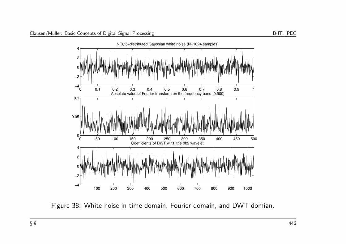
Clausen/Muller: Basic Concepts of Digital Signal Processing B-IT, IPEC
0 0.1 0.2 0.3 0.4 0.5 0.6 0.7 0.8 0.9 1−4
−2
0
2
4N(0,1)−distributed Gaussian white noise (N=1024 samples)
0 50 100 150 200 250 300 350 400 450 5000
0.05
0.1Absolute value of Fourier transform on the frequency band [0:500]
100 200 300 400 500 600 700 800 900 1000−4
−2
0
2
4Coefficients of DWT w.r.t. the db2 wavelet
Figure 38: White noise in time domain, Fourier domain, and DWT domian.
§ 9 446

Clausen/Muller: Basic Concepts of Digital Signal Processing B-IT, IPEC
White noise is characterized by the fact that all frequencies (im the statistical sense)
appear with the same energy. This is also illustrated by the second line of Figure 38 which
shows the absolute values of the Fourier transform: no frequency band is distinguished
from the others. Also in the frequency domain the noise looks like noise.
This observation can also be made when transforming the noise signal by some orthogonal
DWT. The last line of Figure 38 shows the wavelet coefficients of the noise signal
computed on the first M = 10 scales w.r.t. the db2 wavelet. Here the M sequences
w1, w2, . . . , wM and the sequence vM are — as in Equation (68) of Chapter 8 —
written as one sequence
w := (vM, w
M, w
M−1, . . . , w
1),
where the length of this sequence is about the same as for the noise signal (N = 1024).
Note that again the sequence w of wavelet coefficients looks just as noisy as the noise
signal itself. The energy of the white noise is uniformly distributed over all wavelet
coefficients; there is no concentration of the energy in a small number of wavelet
coefficients.
§ 9 447

Clausen/Muller: Basic Concepts of Digital Signal Processing B-IT, IPEC
9.1.2 Thresholding
Donoho describes in [Donoho] two methods to remove “disturbing” wavelet coefficients.
(1) In the so-called hard thresholding method all coefficients are set to zero whose
absolute value lie below a given threshold δ. Hard thresholding can be defined as a
function Thard on input coefficients c:
Tδhard(c) :=
c if |c| ≥ δ
0 if |c| < δ.
(2) The so-called soft thresholding is an extension of hard thresholding. Again all
coefficients are set to zero whose absolut value lie below a given threshold δ. However,
this time all other coefficients are also modified such that their absolute values reduces
by δ. This procedure is also known as wavelet shrinkage. Soft thresholding is defined
§ 9 448

Clausen/Muller: Basic Concepts of Digital Signal Processing B-IT, IPEC
by the function
Tδsoft(c) :=
sign(c)(|c| − δ) if |c| ≥ δ
0 if |c| < δ.
§ 9 449

Clausen/Muller: Basic Concepts of Digital Signal Processing B-IT, IPEC
The two functions T δhard and T δsoft(c) are also shown in Figure 39.
c c c
Without thresholding
−δ
+δ
−δ
+δ
Hard thresholding Soft thresholding
Figure 39: Hard and Soft-Thresholding.
§ 9 450
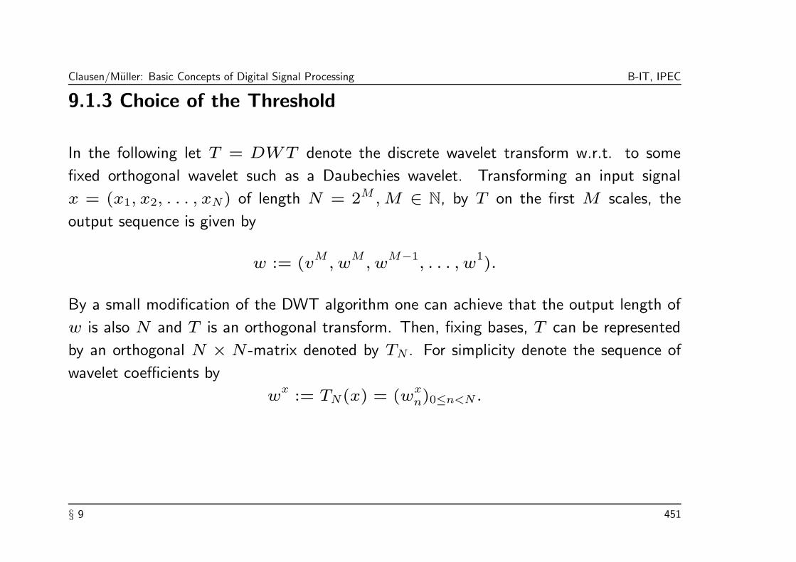
Clausen/Muller: Basic Concepts of Digital Signal Processing B-IT, IPEC
9.1.3 Choice of the Threshold
In the following let T = DWT denote the discrete wavelet transform w.r.t. to some
fixed orthogonal wavelet such as a Daubechies wavelet. Transforming an input signal
x = (x1, x2, . . . , xN) of length N = 2M ,M ∈ N, by T on the first M scales, the
output sequence is given by
w := (vM, w
M, w
M−1, . . . , w
1).
By a small modification of the DWT algorithm one can achieve that the output length of
w is also N and T is an orthogonal transform. Then, fixing bases, T can be represented
by an orthogonal N × N -matrix denoted by TN . For simplicity denote the sequence of
wavelet coefficients by
wx
:= TN(x) = (wxn)0≤n<N .
§ 9 451

Clausen/Muller: Basic Concepts of Digital Signal Processing B-IT, IPEC
As in subsection 9.1.1 we use again the model assumption
s(n) = f(n) + σe(n).
We recall that a N (0, 1)-distributed noise signal (e(n))n∈Z transforms again into a
N (0, 1)-distributed noise signal under some orthogonal transform. Therefore, the wavelet
coefficients we(n) are also uncorrelated N (0, 1)-distributed random variables.
Comparing the wavelet coefficients ws(n) of the noisy signal s with the wavelet
coefficients wf(n) of the original signal, the expected deviation is σ in a statistical sense,
namely the standard deviation of the RV
ws(n) − w
f(n) = σw
e(n).
Therefore, the δ := σ would be a good choice for the threshold δ. Actually, one can
show that this choice in the hard thresholding procedure leads in a statistical sense (w.r.t.
to the so-called risk measure) to an optimally denoised signal f ∗.
§ 9 452

Clausen/Muller: Basic Concepts of Digital Signal Processing B-IT, IPEC
In practice, however, we have to deal with a completely different situation: neither the
original signal f , nor the kind of noise and the noise level σ are known. The only
information we have on hand is the noisy signal s.
In the following, we assume that the noise signal is an N (0, 1)-distributed white noise.
In many applications this is a good model, even though an idealistic assumption. (Note
that there are also many applications where this assumption does not reflect the kind of
noise one has to cope with!)
Then the noise level σ has to be estimated and the threshold δ has to be suitably chosen.
Estimation of parameters such as σ is itself a complicated problem with no standard
solution. The concepts of estimators is part of probability theory. For details on this topic
we have to refer to the literature.
§ 9 453

Clausen/Muller: Basic Concepts of Digital Signal Processing B-IT, IPEC
Some procedures to estimate the noise level δ have been implemented in Matlab (see
thselect). Among others there are
• Steins unbiased estimate of risk (quadratic loss function). This leads to the so-called
SURE thresholding.
• Minimax estimators.
• Combination of methods.
Under the assumption that such a method is at hand, we now want to describe the actual
thresholding algorithm.
§ 9 454

Clausen/Muller: Basic Concepts of Digital Signal Processing B-IT, IPEC
9.1.4 Algorithm for Denoising
Given: Digital noisy signal s with N sampling values.
Possibly information on the properties of the original signal (the original signal is in
general not known, but one often can assume that the original signal lies in some signal
class, e.g., possessing some smoothness properties.
Assumption: The noise component is modelled by an N (0, 1)-distributed Gaussian
white noise.
Parameters: Choice of a suitable wavelet on which bases the DWT is performed.
Choice of a suitable threshold δ by means of some estimator described above.
Choice of thresholding method (hard or soft).
§ 9 455
Clausen/Muller: Basic Concepts of Digital Signal Processing B-IT, IPEC
In view of the anticipated properties of the original signal one chooses suitable parameters.
Note that this choice depends on the respective application. The denoising algorithm
proceeds in three steps:
(1) Transform the noisy signal s by means of the DWT. In the wavelet domain this signal
is represented by the wavelet coefficients (ws(n)).
(2) Apply hard or soft thresholding with threshold δ on the wavelet coefficients (signal
processing in the transform domain).
(3) Reconstruct the signal from the so modified wavelet coefficients (inverse DWT) and
obtain the denoised signal f ∗.
This algorithm can be implemented in Matlab as follows. The Examples in Subsection 5
were generated by such a program.
§ 9 456

Clausen/Muller: Basic Concepts of Digital Signal Processing B-IT, IPEC
%DWT-based Denoising by Thresholding implemented in MATLAB
clear;
N=1024; %number of samples
t=1:N;
wavelet=’db8’; %wavelet
M=floor(log2(N)); %number of scales
e = randn(1,N); %white N(0,1)-distributed noise
sigma = 0.3; %noise level sigma
f=sin(50*pi*(t/N)^ 2) %original signal (chirp signal)
s=f+sigma*e; %noisy signal
thr=thselect(s,’rigrsure’); %threshold
§ 9 457

Clausen/Muller: Basic Concepts of Digital Signal Processing B-IT, IPEC
%DWT of s, wavelet coefficients are w
[w,l]=wavedec(s,M,wavelet);
%hard thresholding, modified wavelet coefficients are whard
whard=w;
for k=(l(1)+1):length(whard),
if abs(whard(k))<=thr whard(k)=0; end
end
%soft thresholding, modified wavelet coefficients are wsoft
wsoft=whard;
for k=(l(1)+1):length(wsoft),
if wsoft(k)<>0 wsoft(k)=sign(wsoft(k))*(abs(wsoft(k))-thr);end
end
§ 9 458

Clausen/Muller: Basic Concepts of Digital Signal Processing B-IT, IPEC
%reconstruction, denoised signal fhard and fsoft
fhard = wrcoef(’a’,whard,l,wavelet,0);
fsoft = wrcoef(’a’,wsoft,l,wavelet,0);
%plot original signal f, noisy signal s and
%denoised signals fhard, fsoft
subplot(4,1,1); plot(t,f); title(’original signal f’)
subplot(4,1,2); plot(t,s); title(’noisy signal s’)
subplot(4,1,3); plot(t,fhard); title(’denoised signal fhard’)
subplot(4,1,4); plot(t,fsoft); title(’denoised signal fsoft’)
The result of this program is shown in the left column of Figure 40.
§ 9 459

Clausen/Muller: Basic Concepts of Digital Signal Processing B-IT, IPEC
9.1.5 Examples for Denoising
In this example, the original signal f is a chirp signal as shown in Figure 40. A DWT was
performed w.r.t. to the db8 wavelet. As described before, the output data is written as
one sequence
w := (vM, w
M, w
M−1, . . . , w
1),
where wm, m = 1, 2, . . . ,M , denote the sequences of wavelet coefficients of scale m,
vM denotes the sequence of scaling coefficients of scale M We recall that the sequence
wm has roughly the length N · 2−m.
The right column of Figure 40 shows the sequence w. Note there are only few wavelet
coefficients of f which have large absolute value. In other words, the energy of f is
concentrated in few wavelet coefficients.
§ 9 460

Clausen/Muller: Basic Concepts of Digital Signal Processing B-IT, IPEC
−2
0
2Orginal signal f
−10
0
10DWT coefficients of f
−2
0
2Noisy signal s
−10
0
10DWT coefficients of s
−2
0
2
Denoised signal f*hard
−10
0
10Hard thresholding with δ=1.7569
200 400 600 800 1000−2
0
2
Denoised signal f*soft
f(t) =sin(50π(t/N)2), N = 1024, M = 10, σ = 0.3, wavelet = db8200 400 600 800 1000
−10
0
10Soft thresholding with δ=1.7569
Figure 40: Denoising of a noisy chirp signal.
§ 9 461

Clausen/Muller: Basic Concepts of Digital Signal Processing B-IT, IPEC
From the illustration of the DWT of the noisy signal s one recognizes that the noisy
component σe results in many wavelet coefficients on all scales of small absolute value.
Using the SURE procedure, the threshold δ was chosen (note that only s is known, but
not f , e or σ). Using hard thresholding and soft thresholding the wavelet coefficients of
the noisy signal were modified and from these the signals f ∗hard and f∗
soft, respectively,
reconstructed. The result of this procedure is shown in Figure 40.
The choice of the wavelet db8 was motivated as follows: assuming that the original signal
f is of high regularity (smooth signal), we also picked a wavelet of high regularity, since
smooth properties of the signal can be better synthesized by smooth synthesis functions.
§ 9 462

Clausen/Muller: Basic Concepts of Digital Signal Processing B-IT, IPEC
The last remark is illustrated by the next example. Here, the original signal consists of
some discontinuous part with a peak (left part) and a smooth part (right part). The
thresholding procedure has been applied with two different wavelets: the db16-Wavelet
of high regularity and the discontinuous Haar wavelet of low regularity. The denoising
algorithm w.r.t. to both wavelets is illustrated in Figures 41 and 42, respectively.
As is seen from the right column of Figure 42, the skyline-like part of f is very efficiently
encoded by the Haar wavelet which leads to few, but large wavelet coefficients in the big
scales. However, the smooth sine-like left part of f is only poorly approximated by the
discontinuous Haar wavelets leading to many small wavelet coefficients spread over all
scales. This last fact leads to problems in the denoising procedure: For the noisy signal s
the small wavelet coefficients coming from the original signal f cannot be distinguished
(by means of the amplitude) from the small wavelet coefficients coming from the noise
component σe.
§ 9 463
Clausen/Muller: Basic Concepts of Digital Signal Processing B-IT, IPEC
In the thresholding procedure, all wavelet coefficients are set to zero whose absolute value
lies below the threshold. Therefore, also many wavelet coefficients which actually encode
the sine-like part of f are set to zero. As a result, in the denoised signals f ∗hard and f∗
soft
the skyline-like part is very well reconstruced. The sine-like left part, however, is strongly
distorted or nearly erased.
This example illustrates what can happen, if the original signal and the wavelet used for
the DWT do not have corresponding properties w.r.t. regularity.
Instead of using the Haar wavelet we next use the db16 wavelet — a wavelet of high
regularity. In this case, as is shown in Figure 41, the sine-like right part of f is encoded
very efficiently but not the skyline-like left part of f . For the same reason as above,
now the sine-like part is very well reconstructed in the denoised signals f ∗hard and f∗
soft,
whereas the skyline-like part is considerably distorted. In f ∗soft, even the peak is erased.
In such cases one also speaks from “over-smoothing”.
§ 9 464

Clausen/Muller: Basic Concepts of Digital Signal Processing B-IT, IPEC
−2
0
2Orginal signal f
−10
0
10DWT coefficients of f
−2
0
2Noisy signal s
−10
0
10DWT coefficients of s
−2
0
2
Denoised signal f*hard
−10
0
10Hard thresholding with δ=2.5376
200 400 600 800 1000−2
0
2
Denoised signal f*soft
N = 1024, M = 10, σ = 0.5, wavelet = db16200 400 600 800 1000 1200
−10
0
10Soft thresholding with δ=2.5376
Figure 41: Denoising with wavelet of high regularity (db16 wavelet).
§ 9 465

Clausen/Muller: Basic Concepts of Digital Signal Processing B-IT, IPEC
−2
0
2Orginal signal f
−10
0
10DWT coefficients of f
−2
0
2Noisy signal s
−10
0
10DWT coefficients of s
−2
0
2
Denoised signal f*hard
−10
0
10Hard thresholding with δ=2.1178
200 400 600 800 1000−2
0
2
Denoised signal f*soft
N = 1024, M = 10, σ = 0.5, wavelet = haar200 400 600 800 1000
−10
0
10Soft thresholding with δ=2.1178
Figure 42: Denoising with Haar wavelet.
§ 9 466

Clausen/Muller: Basic Concepts of Digital Signal Processing B-IT, IPEC
9.1.6 Problems and Remarks
First we want to comment on the differences between hard and soft thresholding. In
hard thresholding, the noise component is in general quite well removed; however, in this
procedure many artefacts such as psudo-oscillations and small abrupt distortions may arise
in the reconstructed signal which substantially degrade the quality. These artefacts are
small when measured in the `2-norm (i.e., the `2-distance between f and f∗hard is small),
but they may be responsible that the resulting signal f ∗hard does not have the same
regularity properties as the original signal f .
For that reason, one often uses soft thresholding in the denoising procedure. In this case,
one has to pay with an additional shrinkage of the wavelet coefficients leading to a loss
of the signal’s energy (and therefore a larger `2-distance between f and f∗soft). However,
one can show that the denoised signal f ∗soft lies with high probability in the signal class
concerning the regularity as the original signal f .
§ 9 467

Clausen/Muller: Basic Concepts of Digital Signal Processing B-IT, IPEC
In other words, with high probability f ∗soft is at least as smooth as the original signal f ,
where this assertions holds for a large class of regularity measures (e.g., in the sense of
n-fold differentiability).
The proof of this result and further details can be found in [Donoho].
As in traditional denoising procedures, e.g., by means of lowpass filtering, one has in the
DWT-based approach a trade-off between denoising and “over-smoothing” of the signal.
The larger the threshold δ, the better the denoising. However, at the same time more and
more details of the original signal f are lost.
For example, in Figure 41 the impulse of the original signal f in the denoised signal f ∗soft
is completely erased.
§ 9 468

Clausen/Muller: Basic Concepts of Digital Signal Processing B-IT, IPEC
Finally, we want to indicate some possible refinements of the denoising algorithm. So
far, we have used in the thresholding procedure one global threshold δ for all wavelet
coefficients — independent of the scale m.
For many applications it has turned out to be advantageous, if a scale-dependent
thresholding in the denoising process. In other words, for each scale m, 1 ≤ m ≤ M , a
separate threshold δm is chosen. This idea is based on the following observations:
(1) In practice, the noise signal e may not be a N (0, 1)-distributed Gaussian white noise
where the energy is uniformly spread over all frequencies, but a so-called colored noise
where the energy is only spread over certain frequency bands. Often one deals with
high-frequency noise so that by this noise the wavelet coefficients of low scales (small
details) are affected.
§ 9 469

Clausen/Muller: Basic Concepts of Digital Signal Processing B-IT, IPEC
(2) The perception of the human auditory system depends very much on the frequency
band components of the signal in question. For example, for some relatively smooth
original signal one may not be as uncomfortable with some low-frequency noise as with
some high-frequency noise.
In particular, using results from psychoaccoustics one has achieved considerable progress
in denoising procedures.
One should not lose sight of the actual goal of denoising: the goal is not to extract a
signal from a noisy signal which has nice mathematical properties such as smoothness
(mathematical quality measure). The goal is to extract a signal which, for the human
listener, is sensed as low-noise signal (subjective quality measure).
§ 9 470

Clausen/Muller: Basic Concepts of Digital Signal Processing B-IT, IPEC
9.2 DWT-Based Compression
The DWT-based compression is based on the same principles as the DWT-based denoising
discussed in the last section. Fundamental is the property of the DWT, that the energy
and therefore the essential information of a large class of signals, which are relevant in
practice (such as audio or video signals), is concentrated in a relatively small number of
large wavelet coefficients.
Let f be the signal to be compressed, w1, w2, . . . , wM be the sequences of wavelet
coefficients of the first M scales, and vM the sequence of scaling coefficients of scale M .
§ 9 471

Clausen/Muller: Basic Concepts of Digital Signal Processing B-IT, IPEC
The compression algorithm is based on the following principle: If the signal f is sufficiently
smooth, then for a suitable chosen M only a small number of scaling and wavelet
coefficients are sufficient for a good approximation of f .
Similar to the denoising procedure, the compression algorithm consists of three steps:
(1) Transform the signal f by the DWT w.r.t. to some suitably chosen wavelet.
(2) Apply thresholding on the wavelet and scaling coefficients (signal processing in the
DWT domain).
(3) By the inverse DWT an approximation of the original signal can be reconstructed.
§ 9 472

Clausen/Muller: Basic Concepts of Digital Signal Processing B-IT, IPEC
• Suppose the original signal f is given by a vector of length N . Applying the DWT one
obtains about the same number of scaling and wavelet coefficients.
• By thresholding the number of non-zero coefficients can be reduced dramatically
depending on the signal class.
• For the reconstructed signal f c it suffices to store these non-zero coefficients together
with some additional information such as the wavelet used in the DFT and the scale
and translation parameters of the non-zero coefficients.
• In other words, storing the approximation f c in the transform domain is much cheaper
than storing the original signal f which amounts in a (lossy) compression of f .
For the compression algorithm there are two strategies. In the first strategy, one uses a
single threshold δ for all scaling and wavelet coefficients. In the second strategy, one uses
different thresholds depending on the respective scale of the coefficients.
§ 9 473

Clausen/Muller: Basic Concepts of Digital Signal Processing B-IT, IPEC
In the first strategy, one chooses the largest wavelet and scaling w.r.t. their absolut value
and all other coefficients are set to zero. The number of the non-zero coefficients can be
determined in different ways such as
• Chose a global threshold δ in the thresholding procedure.
• A compression rate is given which is to be achieved (e.g., 1 : 10). Then choose,
according to this rate, the largest coefficients in the DWT domain. For example,
for the compression rate 1 : 10 one sorts the coefficients according to their absolute
value in decreasing order and then pick the first ten percent. The other 90% of the
coefficients are set to zero.
• A bound for the approximation error is given. To be more precise, the `2-performance
of f c relative to f w.r.t. the `2-norm is measured in percent and defined by
||f c||||f || · 100%.
Then the number of coefficients to be stored depends on the given bound of the
`2-performance which has to be exceed by the reconstruction fc.
§ 9 474

Clausen/Muller: Basic Concepts of Digital Signal Processing B-IT, IPEC
In all three cases, the choice of the scaling and wavelet coefficients set to zero depend on
only one parameter (namely, the threshold δ, the compression rate, or the `2-performance).
In the second strategy the threshold is chosen subject to the respective scale. In other
words, one has several thresholds
δ1, δ2, . . . , δM .
Such a strategy is, for example, the so-called Birge-Massart strategy, which is based on
the “adaptive functional estimation in regression or density contexts”. For details we refer
to [Birge/Massart].
§ 9 475

Clausen/Muller: Basic Concepts of Digital Signal Processing B-IT, IPEC
Although this estimation procedure has a complicated mathematical background, it is easy
to implement. Let M ≥ 2 be the number of scales to be computed in the DWT. As usual
`(wM) denotes the length of the sequence wM consisting of the wavelet coefficients of
the highest scale. Furthermore, let α be a real number greater than one and m0 be an
integer with 1 ≤ m0 ≤ M . The numbers m0, `(wM), and α determine the strategy:
• On the scales m0 + 1, . . . ,M the coefficients are not modified, i.e.,
δm0+1 = . . . = δM = 1.
• For the scale m with 1 ≤ m ≤ m0 one picks the km largest (w.r.t. to their absolut
value) wavelet coefficients in wm, where km is defined by
km :=`(wM)
(m0 + 1 −m)α.
In the compression algorithm one often sets the parameter α = 1.5. This strategy is also
used for denoising where one often sets α = 3.
§ 9 476

Clausen/Muller: Basic Concepts of Digital Signal Processing B-IT, IPEC
Finally, the compression algorithm is illustrated by two examples. Figure 43 shows again
a chirp signal f , our favorite example, and the reconstructed signal f c for different
thresholding procedures. Here, we used the smooth db8 wavelet for the DWT.
Using hard thresholding with threshold δ = 1 , 95.2% of the scaling and wavelet
coefficients are set to zero which corresponds to a compression rate of about 1 : 20.
The `2-performance is about 95.7%. This shows that most of the signal’s energy is
concentrated in a relative small number of coefficients in the DWT domain.
As one expect, increasing δ leads to a better compression rate, however at the expense of
the `2-performance.
The interpretation of the example shown Figure 44 is similar.
§ 9 477

Clausen/Muller: Basic Concepts of Digital Signal Processing B-IT, IPEC
−2
0
2Orginal signal f
−10
0
10DWT coefficients of f
−2
0
2fc with rel. l2−perf.: 88.4%, zero coef.: 96.6%
−10
0
10Hard thresholding with δ=2
−2
0
2fc with rel. l2−perf.: 95.7%, zero coef.: 95.2%
−10
0
10Hard thresholding with δ=1
200 400 600 800 1000−2
0
2fc with rel. l2−perf.: 53.9%, zero coef.: 95.2%
f(t) =sin(50π(t/N)2), N = 1024, M = 10, wavelet = db8200 400 600 800 1000
−10
0
10Soft thresholding with δ=1
Figure 43: DWT-based compression of a chirp signal.
§ 9 478

Clausen/Muller: Basic Concepts of Digital Signal Processing B-IT, IPEC
0
1
2
3
4Orginal signal f
−20
0
20
40
60DWT coefficients of f
0
1
2
3
4fc with rel. l2−perf.: 99.86%, zero coef.: 94.9%
−20
0
20
40
60Hard thresholding with δ=0.5
200 400 600 800 10000
1
2
3
4fc with rel. l2−perf.: 99.97%, zero coef.: 82.4%
N = 1024, M = 10, wavelet = db4200 400 600 800 1000
−20
0
20
40
60Hard thresholding with δ=0.1
Figure 44: DWT-based compression of a noisy signal.
§ 9 479
Clausen/Muller: Basic Concepts of Digital Signal Processing B-IT, IPEC
Warning: The excellent `2-performance in our examples should not be overvalued.
Especially in the first example we are dealing with a synthetic signal of high regulartiy.
The explicit knowledge of the signal was used to pick a suitable wavelet as well as to
determine the threshold δ. To put it in an overstated fashion: if one wants to compress
a pure sine wave, the knowledge of the period results in a compression using only one
coefficient — one can just store the period itself using the sine function as analyizing
function. This would result in a fantastic compression rate with perfect `2-performance.
However, typically one wants to compress signals such as natural images or audio signals.
The choice of suitable parameters constitutes a serious problem. Picking the “wrong”
parameters can lead to more or less useless algorithms even though the underlying theory
has not changed.
§ 9 480
Clausen/Muller: Basic Concepts of Digital Signal Processing B-IT, IPEC
When designing algorithms, the set of test signals on which these algorithms are tested and
suitable parameters are investigated play a crucial role. In this testing and optimization
process it often happens that the properties of the (seemingly representative) test data
itself steal in the designing process. In other words, the improvements of the algorithms
may be based on the specific properties of the test data. Applying the same algorithms to
“real data” may lead to an unexpected poor performance.
In this sense, the examples in this script are solely an illustration of the underlying theory
and do not describe the behaviour of the presented algortihms on real data.
§ 9 481

Clausen/Muller: Basic Concepts of Digital Signal Processing B-IT, IPEC
Chapter 10: The Two Dimensional (2D) Case
The techniques presented in the earlier chapters can be generalized to higher dimensions.
If one understands how to generalize the one-dimensional case to the two-dimensional
case, then it is easy to figure out how to generalize to the n-dimensional case n ∈ N.
Therefore, we only discuss the 2D signals as a useful special case.
As was already mentioned in Chapter 1, two-dimensional signals are important in image
rendering. In this case the two parameters express spatial information. However, a signal’s
two dimension need not be spatial. For example, some filtering techniques work in time
and one spatial dimension.
§ 10 482
Clausen/Muller: Basic Concepts of Digital Signal Processing B-IT, IPEC
10.1 2D-Signals and Systems
To make the analogy between the 1D case and the 2D case as explicit as possible, we use
a straightforward generalization of the notation.
A 2D complex-valued continuous-time (CT) signal is given by a function
f : R2 → C.
For the two arguments we use the symbols t1 and t2.
A 2D complex-valued discrete-time (DT) signal is given by a function
x : Z2 → C.
For the two arguments we use the symbols n1 and n2, k1 and k2, etc.
As for the 1D case, the symbols f, g, . . . are typically used to denote CT-signals whereas
the symbols x, y, . . . are typically used to denote DT-signals.
§ 10 483

Clausen/Muller: Basic Concepts of Digital Signal Processing B-IT, IPEC
Example 10.1. The discrete time unit impulse δ in the 1D case (see Example 1.6)
generalizes to the 2D unit impulse, also denoted by δ, as follows:
δ(n1, n2) :=
1 if n1 = n2 = 0,
0 if n1, n2 6= 0.
As with the one-dimensional case, an arbitrary time-discrete 2D signal x : Z2 → C can
be expressed as a linear combination of shifted unit impulses:
x(n1, n2) =∑
k1∈Z
∑
k2∈Z
x(k1, k2)δ(n1 − k1, n2 − k2).
Example 10.2. The discrete-time unit step function u in the 1D case (see Example 1.7)
generalizes to the 2D unit step function, also denoted by u, as follows:
u(n1, n2) :=
1 if n1 ≥ 0, n2 ≥ 0,
0 otherwise
§ 10 484

Clausen/Muller: Basic Concepts of Digital Signal Processing B-IT, IPEC
Example 10.3. A 2D exponential signal is of the form
an1b
n2
for a, b ∈ R and the 2D sinusoidal signal is of the form
A cos(ω1n1 + φ1) cos(ω2n2 + φ2)
with amplitude A ∈ R, frequencies ω1, ω2 ∈ R, and phases φ1, φ2 ∈ R.
Definition 10.4. A two-dimensional signal is called separable if it can be expressed as a
product of one-dimensional signals. To be more precise, x : Z2 → C is separable if it can
be expressed in the form
x(n1, n2) = x1(n1)x2(n2), n1, n2 ∈ Z,
for suitable 1D signals x1 and x2. An analog definition applies for CT-time signals
f : R2 → C.
It is easy to see that the signals in the Examples 10.1 to 10.3 are separable.
§ 10 485

Clausen/Muller: Basic Concepts of Digital Signal Processing B-IT, IPEC
Completely analog to the 1D case one can define the Lebesgue spaces `p(Z2) for DT
signals and Lp(R2) for CT signals, 1 ≤ p ≤ ∞. For example,
`p(Z) :=
x: Z
2 → C
∣∣∣∑
n1∈Z
∑
n2∈Z
|x(n1, n2)|p < ∞.
or
Lp(R
2) :=
f : R
2 → C
∣∣∣ f measurable and
∫
R
∫
R
| f(t1, t2)|pdt1dt2 < ∞
for 1 ≤ p < ∞. From this it should be clear how to define the corresponding norms (and
the inner products in the case p = 2).
Again the spaces `p(Z2) and Lp(R2) are Banach spaces for 1 ≤ p ≤ ∞. In the case
p = 2 one obtains Hilbert spaces.
§ 10 486

Clausen/Muller: Basic Concepts of Digital Signal Processing B-IT, IPEC
In Chapter 3, a system
T : I → O
was defined for a general space I of input signals and space O of output signals. For
linear spaces I and O the system was called linear if
T [x+ y] = T [x] + T [y] and T [λx] = λT [x],
for all x, y ∈ I and all λ ∈ C (see Definition 3.1). In case I and O are normed spaces, T
is called continuous if it maps all convergent sequences of input signals in I to convergent
sequences of output signals in O.
§ 10 487

Clausen/Muller: Basic Concepts of Digital Signal Processing B-IT, IPEC
Since the spaces `p(Z2) are normed vector spaces, all these concepts can be applied for
systems
T : `p(Z
2) → `
r(Z
2).
As in Definition 3.11 such a system is called time invariant or shift invariant if
T τk1,k2 = τk1,k2 T
for k1, k2 ∈ Z. Here, τk1,k2 denotes the 2D shift operator defined by
τk1,k2[x](n1, n2) := x(n1 − k1, n2 − k2).
For short, a linear time invariant system T : `p(Z2) → `r(Z2) is again simply called an
LTI-system.
§ 10 488

Clausen/Muller: Basic Concepts of Digital Signal Processing B-IT, IPEC
As for the 1D case, a continuous LTI-systems can be easily described and characterized
by the convolution operator. In the 2D case, the convolution x ∗ y of two signals
x, y: Z2 → C is defined by
(x ∗ y)(n1, n2) :=∑
k1∈Z
∑
k2∈Z
x(k1, k2)y(n1 − k1, n2 − k2).
The convolution product only exists with additional assumptions on the signals just as in
the 1D case (see Theorem 3.13). For example, let p and q be conjugated exponents, then
for a fixed y ∈ `q(Z2) the convolution operator
Cy: `p(Z
2) → `
∞(Z
2)
defined by
Cy(x) := x ∗ y, x ∈ `p(Z
2)
defines a linear and continuous operator.
§ 10 489

Clausen/Muller: Basic Concepts of Digital Signal Processing B-IT, IPEC
Then, also in the 2D case, a continuous LTI-System T : `p(Z2) → `q(Z2) is characterized
by its impulse response
h := T [δ].
In particular, one has T [x] = h ∗ x for all x ∈ `p(Z2), i.e., T = Ch. For a stable
LTI-system, i.e., T [δ] ∈ `1(Z2), one obtains the following analog result to Theorem 3.20.
Theorem 10.5. For a linear system T : `p(Z2) → `p(Z2) the following is equivalent:
(1) T is a stable LTI-system.
(2) There is an h ∈ `1(Z2) with T = Ch.
It is straightforward to transfer notions such as FIR filter, IIR filter, causality, etc. from
the 1D to the 2D case.
§ 10 490

Clausen/Muller: Basic Concepts of Digital Signal Processing B-IT, IPEC
10.2 2D Fourier Transform
The Fourier transform, in both continuous-time and discrete-time cases, can be directly
generalized to two dimensions. The only conceptual change is that we now project a 2D
signal onto a set of 2D basis functions. The practical result is that the summations and
integrals become double summations and double integrals.
§ 10 491

Clausen/Muller: Basic Concepts of Digital Signal Processing B-IT, IPEC
10.2.1 2D Fourier Transform for CT-Signals
In the 1D case, a signal can be represented as weighted superposition of the frequency
functions
t 7→ e2πiωt
, t ∈ R,
of frequency ω ∈ R where the weights are given by the Fourier coefficients f(ω). In the
2D case, one uses for the analysis of the signal the following 2D frequency functions:
(t1, t2) 7→ e2πiω1t1e
2πiω2t2 = e2πi(ω1t1+ω2t2)
, t1, t2 ∈ R,
where ω1 ∈ R is the frequency in the first and ω2 ∈ R the frequency in the second
dimension.
§ 10 492

Clausen/Muller: Basic Concepts of Digital Signal Processing B-IT, IPEC
Theorem 2.5 and Definition 2.7 for 1D signals generalizes as follows:
Theorem 10.6. For each signal f ∈ L1(R2) ∩ L2(R2) holds the equality
f(t1, t2) =
∫
R
∫
R
cω1,ω2e
2πi(ω1t1+ω2t2)dω1dω2 (71)
where cω1,ω2is defined by
cω1,ω2=
∫
R
∫
R
f(t1, t2)e−2πi(ω1t1+ω2t2)
dt1dt2. (72)
Definition 10.7. Let f ∈ L1(R2) then the function f : R2 → C defined by
f(ω1, ω2) := cω1,ω2=
∫
R
∫
R
f(t1, t2)e−2πi(ω1t1+ω2t2)
dt1dt2, ω1, ω2 ∈ R,
is called Fourier integral or Fourier transform of f .
§ 10 493
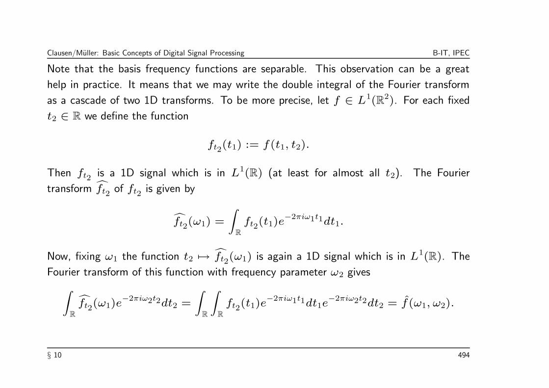
Clausen/Muller: Basic Concepts of Digital Signal Processing B-IT, IPEC
Note that the basis frequency functions are separable. This observation can be a great
help in practice. It means that we may write the double integral of the Fourier transform
as a cascade of two 1D transforms. To be more precise, let f ∈ L1(R2). For each fixed
t2 ∈ R we define the function
ft2(t1) := f(t1, t2).
Then ft2 is a 1D signal which is in L1(R) (at least for almost all t2). The Fourier
transform ft2 of ft2 is given by
ft2(ω1) =
∫
R
ft2(t1)e−2πiω1t1dt1.
Now, fixing ω1 the function t2 7→ ft2(ω1) is again a 1D signal which is in L1(R). The
Fourier transform of this function with frequency parameter ω2 gives
∫
R
ft2(ω1)e−2πiω2t2dt2 =
∫
R
∫
R
ft2(t1)e−2πiω1t1dt1e
−2πiω2t2dt2 = f(ω1, ω2).
§ 10 494

Clausen/Muller: Basic Concepts of Digital Signal Processing B-IT, IPEC
The last equation has important practical ramifications.
• It tells us that we can take a 2D Fourier transform of a signal by taking two successive
1D passes: first transforming all the “rows” (fixing the second variable t2) and then all
the “columns” (fixing the first variable t1).
• Interchanging the role of t1 and t2, the 2D Fourier transform may also be computed
by first transforming all the “columns” and then all the “rows”.
• The synthesis formula shares this property.
• Because of this property, the 2D Fourier transform inherits all the properties of the 1D
transform, such as scaling, convolution, modulation, and so forth.
§ 10 495

Clausen/Muller: Basic Concepts of Digital Signal Processing B-IT, IPEC
Example 10.8. The box function bW from Example 1.2 has a 2D version denoted by
bW1,W2and defined by
bW1,W2(t1, t2) :=
1 if |t1| ≤ W1/2 and |t2| ≤ W2/2
0 otherwise.
Before we take the Fourier transform we will pause for a moment to consider what to
expect. The box function bW1,W2is a separable function, built from the product of two
1D boxes. We know that the Fourier transform of a box is a sinc-function (see Example
2.16), and we saw above that a 2D transform may be taken as a sequence of two 1D
transforms. Intuitively, we would expect the horizontal pass to spread out the horizontal
box into a sinc, and the vertical pass to do the same. Thus we would expect the Fourier
transform of the 2D box to be the product of two 1D sinc functions, one along each axis.
§ 10 496

Clausen/Muller: Basic Concepts of Digital Signal Processing B-IT, IPEC
To confirm this analysis, we find the transform directly, starting with Definition 10.7:
bW1,W2(ω1, ω2) =
∫
R
∫
R
bW1,W2(t1, t2)e
−2πi(ω1t1+ω2t2)dt1dt2
=
∫ W1/2
−W1/2
∫ W2/2
−W2/2
e−2πiω1t1e
−2πiω2t2dt1dt2
=
∫ W1/2
−W1/2
e−2πiω1t1dt1
∫ W2/2
−W2/2
e−2πiω2t2dt2
= W1W2 sinc (W1ω1)sinc (W2ω2).
Figure 45 shows the 2D box function and its Fourier transform. The first line shows a 3D
plot of f and f . In the second line f and f are represented by an image, where the value
of f at (t1, t2) and f at (ω1, ω2) is indicated by the gray level, where smaller values
correspond to dark pixels and larger values to bright pixels.
§ 10 497
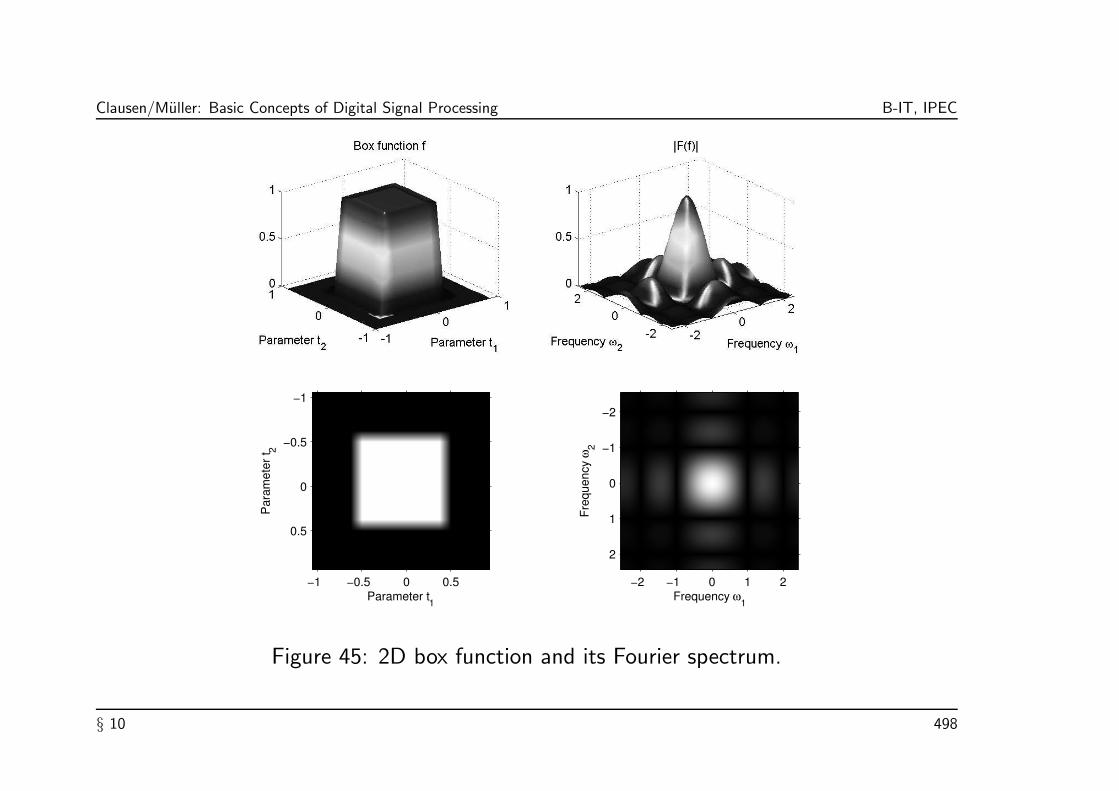
Clausen/Muller: Basic Concepts of Digital Signal Processing B-IT, IPEC
Parameter t1
Par
amet
er t 2
−1 −0.5 0 0.5
−1
−0.5
0
0.5
Frequency ω1
Freq
uenc
y ω
2−2 −1 0 1 2
−2
−1
0
1
2
Figure 45: 2D box function and its Fourier spectrum.
§ 10 498
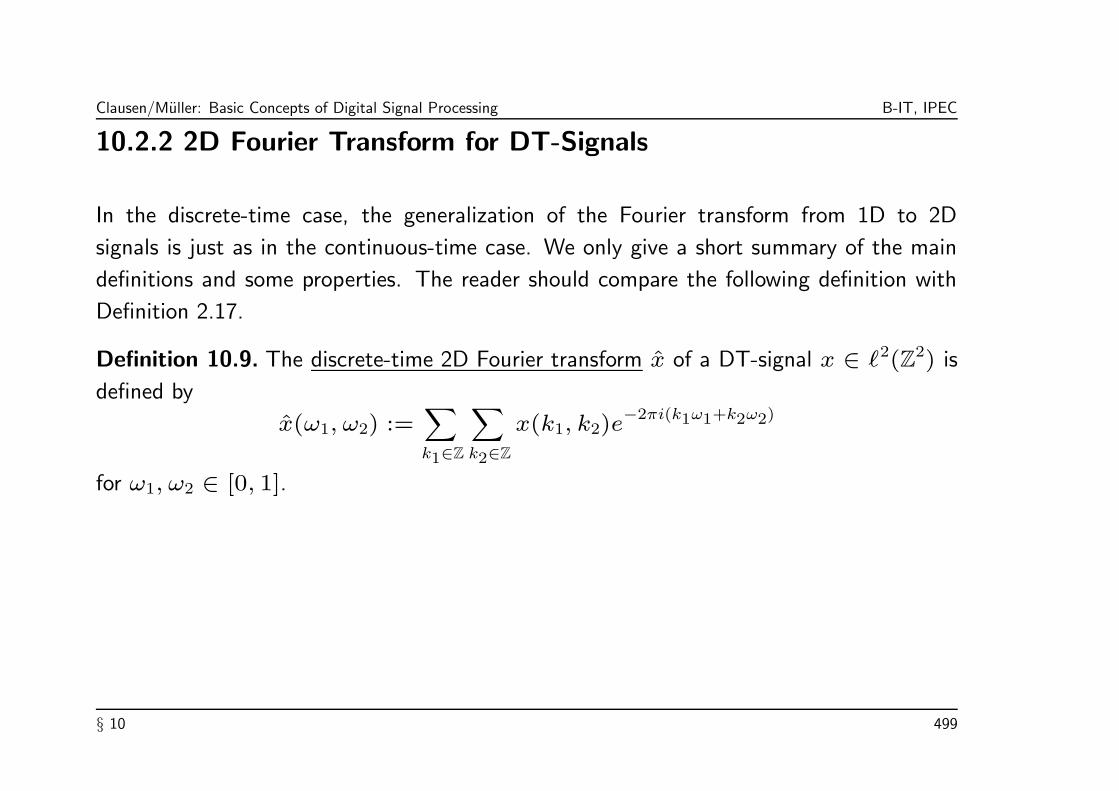
Clausen/Muller: Basic Concepts of Digital Signal Processing B-IT, IPEC
10.2.2 2D Fourier Transform for DT-Signals
In the discrete-time case, the generalization of the Fourier transform from 1D to 2D
signals is just as in the continuous-time case. We only give a short summary of the main
definitions and some properties. The reader should compare the following definition with
Definition 2.17.
Definition 10.9. The discrete-time 2D Fourier transform x of a DT-signal x ∈ `2(Z2) is
defined by
x(ω1, ω2) :=∑
k1∈Z
∑
k2∈Z
x(k1, k2)e−2πi(k1ω1+k2ω2)
for ω1, ω2 ∈ [0, 1].
§ 10 499

Clausen/Muller: Basic Concepts of Digital Signal Processing B-IT, IPEC
Note 10.10. In the 2D case, the Fourier transform x is a (1, 1)-periodic function meaning
that it is 1-periodic w.r.t. to both parameters t1 and t2:
x(ω1 + n1, ω2 + n2) = x(ω1, ω2)
for all n1, n2 ∈ Z and all ω1, ω2 ∈ R. The space of (1, 1)-periodic functions
square-integrable over [0, 1]2 can be identified with the Hilbert space L2([0, 1]2) just as
in the 1D case. One can show that for a DT signal x ∈ `2(Z2), the Fourier transform is
square-integrable over [0, 1]2, i.e., x ∈ L2([0, 1]2).
Lemma 10.11. The signal x ∈ `2(Z2) can be reconstructed from its Fourier transform
x via
x(k1, k2) =
∫
[0,1]
∫
[0,1]
x(ω1, ω2)e−2πi(k1ω1+k2ω2)
dω1dω2.
§ 10 500

Clausen/Muller: Basic Concepts of Digital Signal Processing B-IT, IPEC
As for the 1D case, the frequency response of a 2D convolution filter is defined as 2D
Fourier transform of the filter coefficients. To be more precise, let h := T [δ] ∈ `1(Z2)
be the impulse response of a stable continuous LTI system T , then the frequency response
H of T is defined by
H(ω1, ω2) := h(ω1, ω2) =∑
k1∈Z
∑
k2∈Z
h(k1, k2)e−2πi(k1ω1+k2ω2)
.
As in the 1D case, discrete filters and DT-signals are often denoted by small letters
f, g, h, . . . , x, y . . . and the corresponding Fourier transforms are then denoted by the
corresponding capital letters F,G,H, . . . , X, Y . . ..
§ 10 501

Clausen/Muller: Basic Concepts of Digital Signal Processing B-IT, IPEC
• It can be shown that if h is separable, then H is separable as well, i.e., it can be
expressed in the form
H(ω1, ω2) = H1(ω1)H2(ω2).
• The filter coefficients h(k1, k2) can be recovered from the frequency response as
indicated in Lemma 10.11.
• By applying the Fourier transform on the convolution y = T [x] = h ∗ x, it follows
that the Fourier transforms of the input signal x and the output signal y of a
two-dimensional LTI system are related by
Y (ω1, ω2) = H(ω1, ω2)X(ω1, ω2),
for ω1, ω2 ∈ R.
It is the last property which allows to characterize some LTI system T by means of its
frequency response H: depending on the properties of the magnitude response |H| one
distinguishes, as for the 1D case, between lowpass, highpass, and bandpass filters.
§ 10 502

Clausen/Muller: Basic Concepts of Digital Signal Processing B-IT, IPEC
Example 10.12. As an example, we consider the 2D averaging filter. The reader
should compare the 2D case with the 1D case discussed in Subsection 3.6.2. The
2D averaging filters hN1,N2of length (N1, N2) is defined by
hN1,N2(n1, n2) =
1
N1N2if 0 ≤ n1 ≤ N1 − 1 and 0 ≤ n2 ≤ N2 − 1
0 elsewhere.
Clearly, hN1,N2is a separable filter:
hN1,N2(n1, n2) = hN1
(n1)hN2(n2),
where hN1denotes the 1D averaging filter of length N1 and hN2
denotes the 1D averaging
filter of length N2. Therefore, the frequency response HN1,N2of hN1,N2
is given by
HN1,N2(ω1, ω2) = HN1
(ω1)HN2(ω2)
=1
N1N2
sin(πω1N1)
sin(πω1)
sin(πω2N2)
sin(πω2)e−πi((N1−1)ω1+(N2−1)ω2)
.
§ 10 503
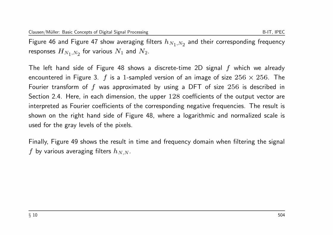
Clausen/Muller: Basic Concepts of Digital Signal Processing B-IT, IPEC
Figure 46 and Figure 47 show averaging filters hN1,N2and their corresponding frequency
responses HN1,N2for various N1 and N2.
The left hand side of Figure 48 shows a discrete-time 2D signal f which we already
encountered in Figure 3. f is a 1-sampled version of an image of size 256 × 256. The
Fourier transform of f was approximated by using a DFT of size 256 is described in
Section 2.4. Here, in each dimension, the upper 128 coefficients of the output vector are
interpreted as Fourier coefficients of the corresponding negative frequencies. The result is
shown on the right hand side of Figure 48, where a logarithmic and normalized scale is
used for the gray levels of the pixels.
Finally, Figure 49 shows the result in time and frequency domain when filtering the signal
f by various averaging filters hN,N .
§ 10 504

Clausen/Muller: Basic Concepts of Digital Signal Processing B-IT, IPEC
Figure 46: Averaging filter hN,N and magnitude response |HN,N | for N = 2, 3, 4.
§ 10 505

Clausen/Muller: Basic Concepts of Digital Signal Processing B-IT, IPEC
Figure 47: Averaging filter hN1,N2and magnitude response |HN1,N2
|.
§ 10 506

Clausen/Muller: Basic Concepts of Digital Signal Processing B-IT, IPEC
Parameter t1
Par
amet
er t 2
50 100 150 200 250
250
200
150
100
50
Frequency ω1
Freq
uenc
y ω
2
−0.5 −0.25 0 0.25 0.5
0.5
0.25
0
−0.25
−0.5
Figure 48: Discrete-time 2D signal f and its approximated Fourier spectrum in decibel
computed by the DFT.
§ 10 507

Clausen/Muller: Basic Concepts of Digital Signal Processing B-IT, IPEC
Signal f
log|F|
f ∗ h4,4
log|F⋅ H4,4
|
f ∗ h8,8
log|F⋅ H8,8
|
f ∗ h16,16
log|F⋅ H16,16
|
Figure 49: Filtered 2D signal f with various averaging filters hN,N in time and spectral
domain.
§ 10 508

Clausen/Muller: Basic Concepts of Digital Signal Processing B-IT, IPEC
10.2.3 2D z-Transform
The z-transform for 1D signals as introduced in Section 3.4 has a straightforward
generalization to the 2D case. For a 2D signal x : Z2 → C, the z-transform X is defined
by
X(z1, z2) =∑
n1∈Z
∑
n2∈Z
x(n1, n2)z−n11 z
−n22 ,
where z1 and z2 are complex variables. As for the 1D case, we use the same symbol X
to denote the z-transform as well as the Fourier transform. With z1 and z2 expressed in
polar coordinates
z1 = r1e2πiω1 and z2 = r2e
2πiω2
the z-transform can be written as
X(r1e2πiω1, r2e
2πiω2) =∑
n1∈Z
∑
n2∈Z
x(n1, n2)r−n11 r
−n22 e
2πiω1n1e2πiω2n2.
§ 10 509
Clausen/Muller: Basic Concepts of Digital Signal Processing B-IT, IPEC
Thus, as in the 1D case, the 2D z-transform can be interpreted as the 2D Fourier
transform of x multiplied by the 2D exponential sequence
(r−n11 r
−n22 )n1∈Z,n2∈Z.
For |z1| = |z2| = 1, i.e., for r1 = r2 = 1, the z-transform is equal to the Fourier
transform. For convergence of the 2D z-transform we require that the sequence
(x(n1, n2)z−n11 z
−n22 )n1∈Z,n2∈Z be absolutely summable, i.e., that
∑
n1∈Z
∑
n2∈Z
|x(n1, n2)z−n11 z
−n22 | < ∞.
The set of values z1 and z2 for which the 2D z-transform converges defines the
region of convergence.
§ 10 510

Clausen/Muller: Basic Concepts of Digital Signal Processing B-IT, IPEC
A 2D z-transform X is said to be separable if it can be expressed in the form
X(z1, z2) = X1(z1)X2(z2).
It is easy to see thatX is separable only if x is separable, i.e., x(n1, n2) = x1(n1)x2(n2)
for suitable 1D signals x1 and x2. In that case X1 and X2 are the 1D z-transforms of x1
and x2, respectively.
The 2D z-transform of a convolution of two 2D signals is the product of their z-transforms:
y = h ∗ x ⇒ Y (z) = H(z)X(z).
As in one dimension, the z-transform of the 2D impulse response is referred to as the
transfer function of the system.
§ 10 511

Clausen/Muller: Basic Concepts of Digital Signal Processing B-IT, IPEC
10.3 Sampling and Aliasing in 2D
We now turn our attention to sampling in two dimensions. Let f : R2 → C be a
continuous CT-signal. We only consider the case of sampling on a rectangular grid with
periods (T1, T2), T1 > 0, T1 > 0. In this case one obtains a DT-signal x: Z2 → C via
x(n1, n2) := f(n1 · T1, n2 · T2), n1, n2 ∈ Z.
One then also speaks from (T1, T2)-sampling and sampling rate (1/T1, 1/T2) measured
in each of the two dimensions separately.
§ 10 512

Clausen/Muller: Basic Concepts of Digital Signal Processing B-IT, IPEC
Similar to the 1D case, the spectrum x of x is the (1, 1)-periodized spectrum of a scaled
version of the spectrum f . We summarize the result in the following theorem (compare to
Theorem 4.9).
Theorem 10.13. Let f be a continuous function with f ∈ L2(R2) and x be the DT-
signal obtained from f by (T1, T2)-sampling. Then
x(ω1, ω2) =1
T1T2
∑
k1∈Z
∑
k1∈Z
f
(ω1 + k1
T1
,ω1 + k1
T1
)for ω1, ω2 ∈ R.
From this it is not difficult to see how the sampling theorem by Shannon extends to the
2D case. First, we need the 2D version of Definition 4.2.
Definition 10.14. Let Ω1,Ω2 > 0. The CT-signal f ∈ L2(R2) is called
(Ω1,Ω2)-bandlimited if the Fourier transform f vanishes for |ω1| > Ω1 and |ω2| > Ω2:
f(ω1, ω2) = 0 ∀|ω1| > Ω1, |ω2| > Ω2, i.e., suppf ⊂ [−Ω1,Ω1] × [−Ω2,Ω2].
§ 10 513

Clausen/Muller: Basic Concepts of Digital Signal Processing B-IT, IPEC
Then the 2D version of Shannon’s theorem is as follows (compare with Theorem 4.6):
Theorem 10.15. Let f ∈ L2(R2) be an (Ω1,Ω2)-bandlimited function and let x be the
(T1, T2)-sampled version of f with T1 := 12Ω1
and T2 := 12Ω2
, i.e.,
x(n1, n2) := f(n1 · T1, n2 · T2), n1, n2 ∈ Z.
Then f can be reconstructed from x as follows:
f(t1, t2) =∑
n1∈Z
∑
n2∈Z
x(n1, n2)sinc
(t1 − n1T1
T1
)sinc
(t2 − n2T2
T2
).
Note 10.16. Theorem 4.3 and Note 4.4 also apply for the 2D case.
§ 10 514

Clausen/Muller: Basic Concepts of Digital Signal Processing B-IT, IPEC
10.4 2D MRA and Wavelets
In this section, we indicate how to generalize the 1D multiresolution analysis presented
in Chapter 8 following in most part Section 2.2.2 of [Louis/Maaß/Rieder]. We also refer
for further details to this book. The properties of 2D MRAs are the basis for usage of
wavelets in applications such as image analysis and image compression.
A multiresolution analysis of L2(R2) consists — just as for the 1D case — of an increasing
sequence of closed subspaces Vm ⊂ L2(R2), m ∈ Z, such that
⋃
m∈Z
Vm = L2(R
2) and
⋂
m∈Z
Vm = 0.
§ 10 515

Clausen/Muller: Basic Concepts of Digital Signal Processing B-IT, IPEC
In contrast to the 1D MRA, we now admit translates k ∈ Z2 and the transition from Vm
to Vm−1 is described by a regular matrix A, also denoted as dilation matrix:
f(·) ∈ Vm ⇐⇒ f(A·) ∈ Vm−1.
The base space V0 is again generated by an ONB consisting of all integer translates of a
scaling function ϕ ∈ V0:
V0 = spanϕ(· − k)|k ∈ Z2.
Then it follows that
ϕm,k := | detA|−m/2ϕ(Am · −k)|k ∈ Z
2
is an ONB of Vm. According to the philosophy of the MRA decomposition the dilation
matrix should stretch in all directions. In other words, the absolute values of the
eigenvalues of A are greater then one. Furthermore, A should have integer entries. This
is equivalent to
AZ2 ⊂ Z
2.
§ 10 516

Clausen/Muller: Basic Concepts of Digital Signal Processing B-IT, IPEC
2D wavelets are those functions which span the orthogonal complement of V0 in V−1.
This is, in general, not any longer possible for one single function with all its integer
translates. The following heuristic note should convince us of this fact and should motivate
the following theorem of Y. Meyer.
Note 10.17. We chose as scaling function the characteristic function of some set Ω. The
basis functions of V−1 is then the characteristic function of the set A−1Ω with measure
µ(A−1
Ω) = µ(Ω)/| detA|.
A basis of V−1 needs therefore “| detA|-times” the number of elements as a basis of V0.
The orthogonal complement of V0 is in this sense “(| detA| − 1)-times” larger then V0.
§ 10 517

Clausen/Muller: Basic Concepts of Digital Signal Processing B-IT, IPEC
Theorem 10.18. [Meyer.] Let (Vm)m∈Z be an MRA with dilation matrix A. Then
there exist | detA| − 1 wavelets
ψ1, ψ2, . . . , ψ| detA|−1 ∈ V−1
which generate an ONB of the orthogonal complement of V0 in V−1, i.e.,
ψj,m,k = | detA|−m/2ψj(A−m · −k)
∣∣j = 1, 2, . . . | detA| − 1,m ∈ Z, k ∈ Z2
is an ONB of L2(R2).
By this theorem we obtain an orthogonal decomposition of V−1 in | detA| subspaces
V−1 =
| detA|−1⊕
j=1
W0,j ⊕ V0,
where the spaces W0,j are given by
W0,j = spanψj(· − k)|k ∈ Z2.
§ 10 518

Clausen/Muller: Basic Concepts of Digital Signal Processing B-IT, IPEC
Note 10.19. In case of the definition of 1D MRA one may replace the dilation parameter
2 (see condition (35) in Definition 8.1) by some arbitrary integer parameter p ≥ 2. Then,
however, one also needs p− 1 one-dimensional wavelets to generate W0.
As example, we consider the so-called tensor product wavelets. In general, the tensor
product f ⊗ g : R2 → C of two functions f, g : R → C is defined by
f ⊗ g(t1, t2) := f(t1)g(t2).
We start with a 1D orthogonal wavelet ψ and some orthogonal scaling function ϕ coming
from an 1D MRA. Note that the set of functions
ψm,k ⊗ ψµ,κ | m,µ, k, κ ∈ Z
defines an ONB of L2(R2). However, it does not constitute a wavelet basis, since for
m 6= µ the basis functions of different scales are mixed up.
§ 10 519

Clausen/Muller: Basic Concepts of Digital Signal Processing B-IT, IPEC
One has to chose a different approach. The tensor product ϕ⊗ ϕ of the scaling function
ϕ generates a 2D scaling function for a 2D MRA w.r.t. the dilation matrix
A =
(2 0
0 2
).
By Theorem 10.18 there are | detA| − 1 = 3 wavelets whose integer translates form a
basis of W0. One can show that these wavelets are given by
ϕ⊗ ψ, ψ ⊗ ϕ, and ψ ⊗ ψ.
In this basis, there is no mixing up of different scales. A decomposition w.r.t. this basis
has a typical multiresolution property.
§ 10 520

Clausen/Muller: Basic Concepts of Digital Signal Processing B-IT, IPEC
• The 2D wavelets and the scaling function defined by tensor products are obviously
separable functions. Therefore, their properties can easily by deduced from the 1D
case.
• However, there is also a disadvantage concerning these wavelets: one needs three
different wavelets to generate W0.
• The wavelets constructed as above have the property that certain directions (the t1-
and t2-direction as well as the diagonal) are “privileged”. Such wavelets are also
called anisotrop. This property can be an advantage when used for edge detection in
images. However, tensor product wavelets are not suitable in view of applications in
data compression. This application demands isotropy and a number of wavelets as
small as possible.
In view of the last application, one may study 2D MRAs having a dilation matrix A with
| detA| = 2. For further details on this topic we have to refer to the literature such as
[Louis/Maaß/Rieder].
§ 10 521

Clausen/Muller: Basic Concepts of Digital Signal Processing B-IT, IPEC
Literature
[Clausen/Muller] Michael Clausen, Meinard Muller: Zeit-Frequenz-Analyse und
Wavelettransformation. Script, summer term 2001, University of Bonn.
[Blatter] Christian Blatter: Wavelets - Eine Einfuhrung. Vieweg 1998
[Burrus/Gopinath/Guo] C. Sidney Burrus, Ramesh A. Gopinath, Haitao Guo: Wavelets
and Wavelet Transforms. Prentice Hall, New Jersey 1998
[Clausen/Baum] Michael Clausen, Ulrich Baum: Fast Fourier Transforms. BI
Wissenschaftsverlag 1993
[Daubechies] Ingrid Daubechies: Ten lectures on wavelets. CBMS-NSF Regional
Conference Series in Applied Mathematics, SIAM 1992
[Donoho] David L. Donoho: Denoising by Soft-Thresholding. IEEE Transaction on
Information Theory, Vol. 41, Nr. 3, S. 613 - 627, Mai 1995
[Folland] Gerald B. Folland: Real Analysis. John Wiley & Sons, 1984
[Glassner] Andrew S. Glassner: Principles of Digital Image Synthesis. Morgan
Kaufmann Publishers, Inc. 1999
§ 10 522
Clausen/Muller: Basic Concepts of Digital Signal Processing B-IT, IPEC
[Hubbard] Barbara Burke Hubbard: The world according to wavelets. AK Peters,
Wellesley, Massachusetts, 1996
[Kaiser] Gerald Kaiser: A friendly guide to wavelets. Birkhauser 1994
[Krengel] Ulrich Krengel: Einfuhrung in die Wahrscheinlichkeitstheorie und Statistik.
Vieweg, 1991
[Lang] Serge Lang: Algebra. Addison-Wesley Publishing Company, 1993
[Louis/Maaß/Rieder] Alfred K. Louis, Peter Maaß, Andreas Rieder: Waveltes. B. G.
Teubner, Stuttgart 1994
[Matlab] M. Misiti, Y. Misiti, G. Oppenheim J.-M. Poggi: Wavelet Toolbox for Use with
Matlab. The MathWorks, Inc. 1996
[Pohlman] Ken C. Pohlmann: Principles of Digital Audio. McGraw-Hill, Inc. 1995
[Proakis/Manolakis] John G. Proakis, Dimitris G. Manolakis: Digital Signal Processing.
Prentice Hall, 1996
[Oppenheim/Schafer] Alan V. Oppenheim, Ronald W. Schafer: Digital Signal
Processing. VCH, 1975
§ 10 523

Clausen/Muller: Basic Concepts of Digital Signal Processing B-IT, IPEC
[Oppenheim/Willsky] Alan V. Oppenheim, Alan S. Willsky: Signale und Systeme.
VCH, 1992
[Remmert] Remmert: Funktionentheorie 1. 3. Auflage, Springer-Verlag
[Strang/Nguyen] Gilbert Strang, Truong Nguyen: Wavelets and Filter Banks.
Wellesley-Cambridge Press 1996
[Wickerhauser] Mladen V. Wickerhauser: Adaptive Wavelet-Analysis. Vieweg 1993
§ 10 524