Basic Concepts in Matrix Algebra - Iowa State...

Basic Concepts in Matrix Algebra

• An column array of p elements is called a vector of dimension p and iswritten as

xp×1 =

x1x2...xp

.

• The transpose of the column vector xp×1 is row vector

x′ = [x1 x2 . . . xp]

• A vector can be represented in p-space as a directed line with compo-nents along the p axes.

38

Basic Matrix Concepts (cont’d)

• Two vectors can be added if they have the same dimension. Additionis carried out elementwise.

x + y =

x1x2...xp

+

y1y2...yp

=

x1 + y1x2 + y2...xp + yp

• A vector can be contracted or expanded if multiplied by a constant c.Multiplication is also elementwise.

cx = c

x1x2...xp

=

cx1cx2...cxp

39

Examples

x =

21−4

and x′ =[

2 1 −4]

6× x = 6×

21−4

=

6× 26× 1

6× (−4)

=

126

−24

x + y =

21−4

+

5−2

0

=

2 + 51− 2−4 + 0

=

7−1−4

40


• Multiplication by c > 0 does not change the direction of x. Direction isreversed if c < 0.

41


• The length of a vector x is the Euclidean distance from the origin

Lx =

√√√√√ p∑j=1

x2j

• Multiplication of a vector x by a constant c changes the length:

Lcx =

√√√√√ p∑j=1

c2x2j = |c|

√√√√√ p∑j=1

x2j = |c|Lx

• If c = L−1x , then cx is a vector of unit length.

42

Examples

The length of x =

21−4−2

is

Lx =√

(2)2 + (1)2 + (−4)2 + (−2)2 =√

25 = 5

Then

z =1

5×

21−4−2

=

0.40.2−0.8−0.4

is a vector of unit length.

43

Angle Between Vectors

• Consider two vectors x and y in two dimensions. If θ1 is the anglebetween x and the horizontal axis and θ2 > θ1 is the angle betweeny and the horizontal axis, then

cos(θ1) =x1

Lxcos(θ2) =

y1

Ly

sin(θ1) =x2

Lxsin(θ2) =

y2

Ly,

If θ is the angle between x and y, then

cos(θ) = cos(θ2 − θ1) = cos(θ2) cos(θ1) + sin(θ2) sin(θ1).

Then

cos(θ) =x1y1 + x2y2

LxLy.

44

Angle Between Vectors (cont’d)

45

Inner Product

• The inner product between two vectors x and y is

x′y =p∑

j=1

xjyj.

• Then Lx =√x′x, Ly =

√y′y and

cos(θ) =x′y√

(x′x)√

(y′y)

• Since cos(θ) = 0 when x′y = 0 and cos(θ) = 0 for θ = 90or θ = 270, then the vectors are perpendicular (orthogonal) whenx′y = 0.

46

Linear Dependence

• Two vectors, x and y, are linearly dependent if there existtwo constants c1 and c2, not both zero, such that

c1x + c2y = 0

• If two vectors are linearly dependent, then one can be written as alinear combination of the other. From above:

x = (c2/c1)y

• k vectors, x1,x2, . . . ,xk, are linearly dependent if there exist con-stants (c1, c2, ..., ck) not all zero such that

k∑j=1

cjxj = 0

47

• Vectors of the same dimension that are not linearlydependent are said to be linearly independent

Linear Independence-example

Let

x1 =

121

, x2 =

10−1

, x3 =

1−2

1

Then c1x1 + c2x2 + c3x3 = 0 if

c1 + c2 + c3 = 02c1 + 0 − 2c3 = 0c1 − c2 + c3 = 0

The unique solution is c1 = c2 = c3 = 0, so the vectors are linearlyindependent.

48

Matrices

A matrix A is an array of elements aij with n rows and p columns:

A =

a11 a12 · · · a1pa21 a22 · · · a2p... ... . . . ...an1 an2 · · · anp

The transpose A′ has p rows and n columns. The j-th row of A′ is the j-thcolumn of A

A′ =

a11 a21 · · · an1a12 a22 · · · an2... ... . . . ...a1p a2p · · · anp

50

Matrix Algebra

• Multiplication of A by a constant c is carried out element by element.

cA =

ca11 ca12 · · · ca1pca21 ca22 · · · ca2p... ... . . . ...can1 can2 · · · canp

51

Matrix AdditionTwo matrices An×p = {aij} and Bn×p = {bij} of the same dimen-sions can be added element by element. The resulting matrix is Cn×p ={cij} = {aij + bij}

C = A+B

=

a11 a12 · · · a1pa21 a22 · · · a2p... ... . . . ...an1 an2 · · · anp

+

b11 b12 · · · b1pb21 b22 · · · b2p... ... . . . ...bn1 bn2 · · · bnp

=

a11 + b11 a12 + b12 · · · a1p + b1pa21 + b21 a22 + b22 · · · a2p + b2p... ... . . . ...an1 + bn1 an2 + bn2 · · · anp + bnp

52

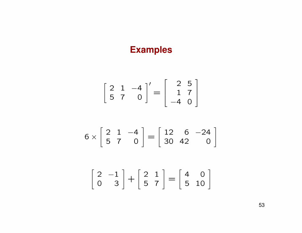
Examples

[2 1 −45 7 0

]′=

2 51 7−4 0

6×[

2 1 −45 7 0

]=

[12 6 −2430 42 0

]

[2 −10 3

]+

[2 15 7

]=

[4 05 10

]

53

Matrix Multiplication

• Multiplication of two matrices An×p and Bm×q can be carried out onlyif the matrices are compatible for multiplication:

– An×p ×Bm×q: compatible if p = m.

– Bm×q ×An×p: compatible if q = n.

The element in the i-th row and the j-th column of A× B is the innerproduct of the i-th row of A with the j-th column of B.

54

Multiplication Examples

[2 0 15 1 3

]×

1 4−1 3

0 2

=

[2 104 29

]

[2 15 3

]×[

1 4−1 3

]=

[1 112 29

]

[1 4−1 3

]×[

2 15 3

]=

[22 1313 8

]

55

Identity Matrix

• An identity matrix, denoted by I, is a square matrix with 1’s along themain diagonal and 0’s everywhere else. For example,

I2×2 =

[1 00 1

]and I3×3 =

1 0 00 1 00 0 1

• If A is a square matrix, then AI = IA = A.

• In×nAn×p = An×p but An×pIn×n is not defined for p 6= n.

56

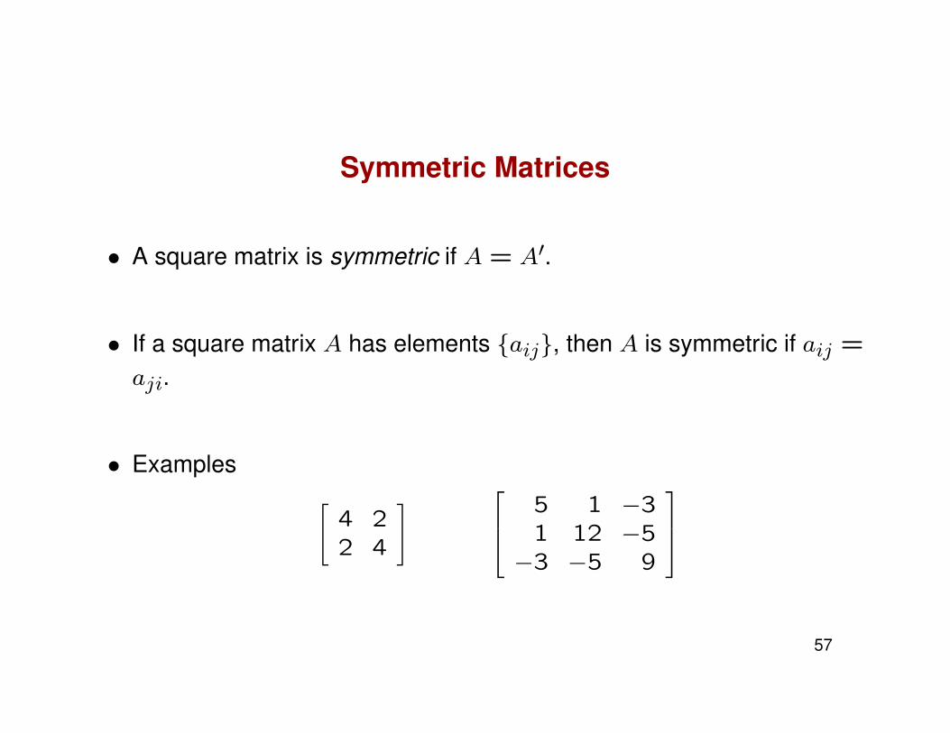
Symmetric Matrices

• A square matrix is symmetric if A = A′.

• If a square matrix A has elements {aij}, then A is symmetric if aij =

aji.

• Examples [4 22 4

] 5 1 −31 12 −5−3 −5 9

57

Inverse Matrix

• Consider two square matrices Ak×k and Bk×k. If

AB = BA = I

then B is the inverse of A, denoted A−1.

• The inverse of A exists only if the columns of A are linearly indepen-dent.

• If A = diag{aij} then A−1 = diag{1/aij}.

58

Inverse Matrix

• For a 2× 2 matrix A, the inverse is

A−1 =

[a11 a12a21 a22

]−1

=1

det(A)

[a22 −a12−a21 a11

],

where det(A) = (a11 × a22)− (a12 × a21) denotes thedeterminant of A.

59

Orthogonal Matrices

• A square matrix Q is orthogonal if

QQ′ = Q′Q = I,

or Q′ = Q−1.

• If Q is orthogonal, its rows and columns have unit length (q′jqj = 1)and are mutually perpendicular (q′jqk = 0 for any j 6= k).

60

Eigenvalues and Eigenvectors

• A square matrix A has an eigenvalue λ with corresponding eigenvec-tor z 6= 0 if

Az = λz

• The eigenvalues of A are the solution to |A− λI| = 0.

• A normalized eigenvector (of unit length) is denoted by e.

• A k × k matrix A has k pairs of eigenvalues and eigenvectors

λ1, e1 λ2, e2 ... λk, ek

where e′iei = 1, e′iej = 0 and the eigenvectors are unique up to achange in sign unless two or more eigenvalues are equal.

61

Spectral Decomposition

• Eigenvalues and eigenvectors will play an important role in this course.For example, principal components are based on the eigenvalues andeigenvectors of sample covariance matrices.

• The spectral decomposition of a k × k symmetric matrix A is

A = λ1e1e′1 + λ2e2e

′2 + ...+ λkeke

′k

= [e1 e2 · · · ek]

λ1 0 · · · 00 λ2 · · · 0... ... . . . ...0 0 · · · λk

[e1 e2 · · · ek]′

= PΛP ′

62

Determinant and Trace

• The trace of a k× k matrix A is the sum of the diagonal elements, i.e.,trace(A) =

∑ki=1 aii

• The trace of a square, symmetric matrix A is the sum of the eigenval-ues, i.e., trace(A) =

∑ki=1 aii =

∑ki=1 λi

• The determinant of a square, symmetric matrix A is the product of theeigenvalues, i.e., |A| =

∏ki=1 λi

63

Rank of a Matrix

• The rank of a square matrix A is

– The number of linearly independent rows

– The number of linearly independent columns

– The number of non-zero eigenvalues

• The inverse of a k × k matrix A exists, if and only if

rank(A) = k

i.e., there are no zero eigenvalues

64

Positive Definite Matrix

• For a k × k symmetric matrix A and a vector x = [x1, x2, ..., xk]′ thequantity x′Ax is called a quadratic form

• Note that x′Ax =∑ki=1

∑kj=1 aijxixj

• If x′Ax ≥ 0 for any vector x, both A and the quadratic form are saidto be non-negative definite.

• If x′Ax > 0 for any vector x 6= 0, both A and the quadratic form aresaid to be positive definite.

65

Example 2.11

• Show that the matrix of the quadratic form 3x21 + 2x2

2 − 2√

2x1x2 ispositive definite.

• For

A =

[3 −

√2

−√

2 2

],

the eigenvalues are λ1 = 4, λ2 = 1. Then A = 4e1e′1 +e2e

′2. Write

x′Ax = 4x′e1e′1x + x′e2e

′2x

= 4y21 + y2

2 ≥ 0,

and is zero only for y1 = y2 = 0.

66

Example 2.11 (cont’d)

• y1, y2 cannot be zero because[y1y2

]=

[e′1e′2

] [x1x2

]= P ′2×2x2×1

with P ′ orthonormal so that (P ′)−1 = P . Then x = Py and sincex 6= 0 it follows that y 6= 0.

• Using the spectral decomposition, we can show that:

– A is positive definite if all of its eigenvalues are positive.

– A is non-negative definite if all of its eigenvalues are ≥ 0.

67

Distance and Quadratic Forms

• For x = [x1, x2, ..., xp]′ and a p× p positive definite matrix A,

d2 = x′Ax > 0

when x 6= 0. Thus, a positive definite quadratic form can be inter-preted as a squared distance of x from the origin and vice versa.

• The squared distance from x to a fixed pointµ is given by the quadraticform

(x− µ)′A(x− µ).

68

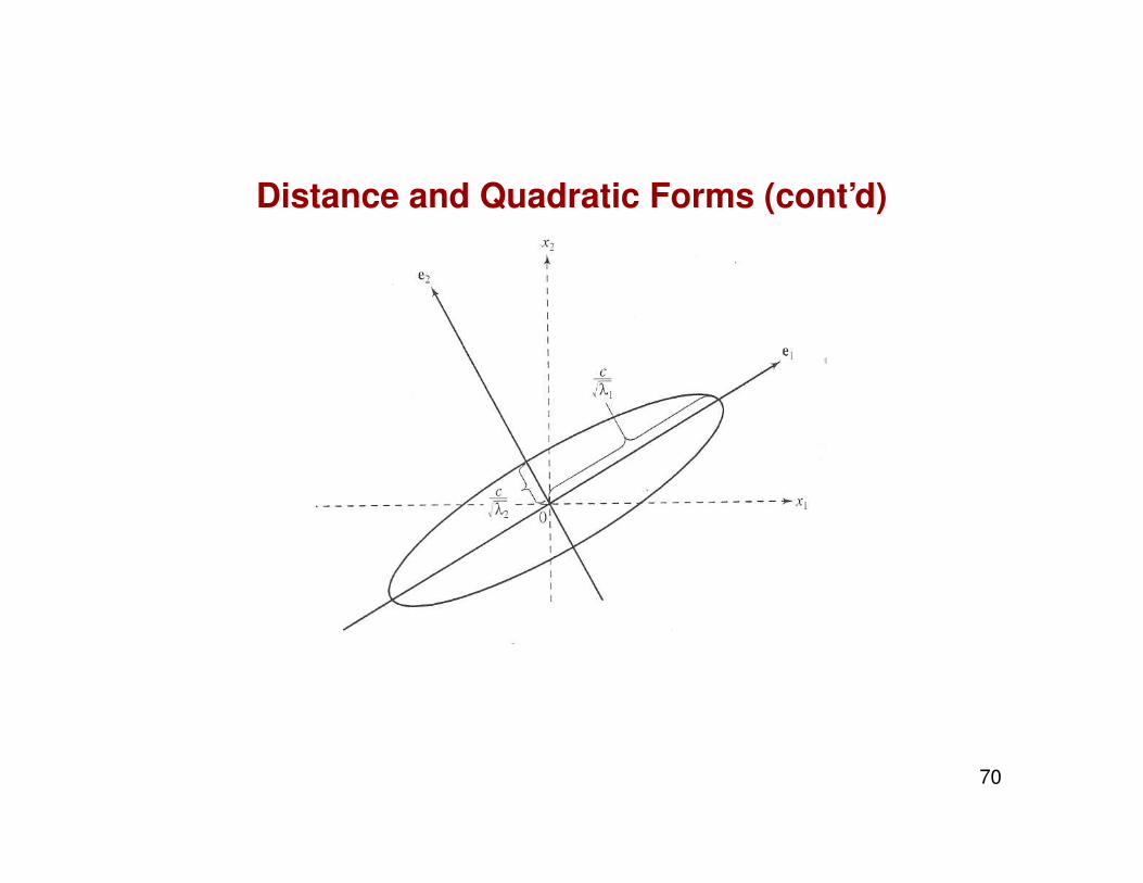
Distance and Quadratic Forms (cont’d)

• We can interpret distance in terms of eigenvalues and eigenvectors ofA as well. Any point x at constant distance c from the origin satisfies

x′Ax = x′(p∑

j=1

λjeje′j)x =

p∑j=1

λj(x′ej)

2 = c2,

the expression for an ellipsoid in p dimensions.

• Note that the point x = cλ−1/21 e1 is at a distance c (in the direction of

e1) from the origin because it satisfies x′Ax = c2. The same is truefor points x = cλ

−1/2j ej, j = 1, ..., p. Thus, all points at distance c lie

on an ellipsoid with axes in the directions of the eigenvectors and withlengths proportional to λ−1/2

j .

69

Distance and Quadratic Forms (cont’d)

70

Square-Root Matrices

• Spectral decomposition of a positive definite matrix A yields

A =p∑

j=1

λjeje′j = PΛP,

with Λk×k = diag{λj}, all λj > 0, and Pk×k = [e1 e2 ... ep] anorthonormal matrix of eigenvectors. Then

A−1 = PΛ−1P ′ =p∑

j=1

1

λjeje′j

• With Λ1/2 = diag{λ1/2j }, a square-root matrix is

A1/2 = PΛ1/2P ′ =p∑

j=1

√λjeje

′j

71

Square-Root Matrices

The square root of a positive definite matrix A has thefollowing properties:

1. Symmetry: (A1/2)′ = A1/2

2. A1/2A1/2 = A

3. A−1/2 =∑pj=1 λ

−1/2j eje

′j = PLambda−1/2P ′

4. A1/2A−1/2 = A−1/2A1/2 = I

5. A−1/2A−1/2 = A−1

Note that there are other ways of defining the square root of a positivedefinite matrix: in the Cholesky decomposition A = LL′, with L a matrixof lower triangular form, L is also called a square root of A.

72

Random Vectors and Matrices• A random matrix (vector) is a matrix (vector) whose elements are ran-

dom variables.

• IfXn×p is a random matrix, the expected value ofX is the n×pmatrix

E(X) =

E(X11) E(X12) · · · E(X1p)E(X21) E(X22) · · · E(X2p)... ... · · · ...E(Xn1) E(Xn2) · · · E(Xnp)

,where

E(Xij) =∫ ∞∞

xijfij(xij)dxij

with fij(xij) the density function of the continuous random variableXij. If X is a discrete random variable, we compute its expectation asa sum rather than an integral.

73

Linear Combinations

• The usual rules for expectations apply. If X and Y are two randommatrices and A and B are two constant matrices of the appropriatedimensions, then

E(X + Y ) = E(X) + E(Y )

E(AX) = AE(X)

E(AXB) = AE(X)B

E(AX +BY ) = AE(X) +BE(Y )

• Further, if c is a scalar-valued constant then

E(cX) = cE(X).

74

Mean Vectors and Covariance Matrices

• Suppose that X is p×1 (continuous) random vector drawn from somep−dimensional distribution.

• Each element of X, say Xj has its own marginal distribution withmarginal mean µj and variance σjj defined in the usual way:

µj =∫ ∞−∞

xjfj(xj)dxj

σjj =∫−∞

(xj − µj)2fj(xj)dxj

75

Mean Vectors and Covariance Matrices (cont’d)

• To examine association between a pair of random variables we needto consider their joint distribution.

• A measure of the linear association between pairs of variables is givenby the covariance

σjk = E[(Xj − µj)(Xk − µk)

]=

∫ ∞−∞

∫ ∞−∞

(xj − µj)(xk − µk)fjk(xj, xk)dxjdxk.

76


• If the joint density function fjk(xj, xk) can be written asthe product of the two marginal densities, e.g.,

fjk(xj, xk) = fj(xj)fk(xk),

then Xj and Xk are independent.

• More generally, the p−dimensional random vector X hasmutually independent elements if the p−dimensional jointdensity function can be written as the product of the punivariate marginal densities.

• If two random variables Xj and Xk are independent, then their covari-ance is equal to 0. [Converse is not always true.]

77


• We use µ to denote the p × 1 vector of marginal population meansand use Σ to denote the p× p population variance-covariance matrix:

Σ = E[(X − µ)(X − µ)′

].

• If we carry out the multiplication (outer product)then Σ is equal to:

E

(X1 − µ1)2 (X1 − µ1)(X2 − µ2) · · · (X1 − µ1)(Xp − µp)

(X2 − µ2)(X1 − µ1) (X2 − µ2)2 · · · (X2 − µ2)(Xp − µp)... ... · · · ...

(Xp − µp)(X1 − µ1) (Xp − µp)(X2 − µ2) · · · (Xp − µp)2

.

78


• By taking expectations element-wise we find that

Σ =

σ11 σ12 · · · σ1pσ21 σ22 · · · σ2p... ... · · · ...σp1 σp2 · · · σpp

.

• Since σjk = σkj for all j 6= k we note that Σ is symmetric.

• Σ is also non-negative definite

79

Correlation Matrix

• The population correlation matrix is the p× p matrix withoff-diagonal elements equal to ρjk and diagonal elementsequal to 1.

1 ρ12 · · · ρ1pρ21 1 · · · ρ2p... ... · · · ...ρp1 ρp2 · · · 1

.

• Since ρij = ρji the correlation matrix is symmetric

• The correlation matrix is also non-negative definite

80

Correlation Matrix (cont’d)

• The p×p population standard deviation matrix V 1/2 is a diagonal ma-trix with√σjj along the diagonal and zeros in all off-diagonal positions.Then

Σ = V 1/2P V 1/2

and the population correlation matrix is

(V 1/2)−1Σ(V 1/2)−1

• Given Σ, we can easily obtain the correlation matrix

81

Partitioning Random vectors

• If we partition the random p×1 vector X into two components X1, X2of dimensions q×1 and (p−q)×1 respectively, then the mean vectorand the variance-covariance matrix need to be partitioned accordingly.

• Partitioned mean vector:

E(X) = E

[X1

X2

]=

[E(X1)

E(X2)

]=

[µ1

µ2

]

• Partitioned variance-covariance matrix:

Σ =

[V ar(X1) Cov(X1, X2)

Cov(X2, X1) V ar(X2)

]=

[Σ11 Σ12

Σ′12 Σ22

],

where Σ11 is q× q, Σ12 is q× (p− q) and Σ22 is (p− q)× (p− q).

82

Partitioning Covariance Matrices (cont’d)

• Σ11,Σ22 are the variance-covariance matrices of thesub-vectors X1, X2, respectively. The off-diagonal elementsin those two matrices reflect linear associations amongelements within each sub-vector.

• There are no variances in Σ12, only covariances. Thesecovariancs reflect linear associations between elementsin the two different sub-vectors.

83

Linear Combinations of Random variables

• Let X be a p × 1 vector with mean µ and variance covariance matrixΣ, and let c be a p×1 vector of constants. Then the linear combinationc′X has mean and variance:

E(c′X) = c′µ, and V ar(c′X) = c′Σc

• In general, the mean and variance of a q×1 vector of linear combina-tions Z = Cq×pXp×1 are

µZ = CµX and ΣZ = CΣXC′.

84

Cauchy-Schwarz Inequality

• We will need some of the results below to derive somemaximization results later in the course.

Cauchy-Schwarz inequality Let b and d be any twop× 1 vectors. Then,

(b′d)2 ≤ (b′b)(d′d)

with equality only if b = cd for some scalar constant c .

Proof: The equality is obvious for b = 0 or d = 0. For other cases,consider b− cd for any constant c 6= 0 . Then if b− cd 6= 0, we have

0 < (b− cd)′(b− cd) = b′b− 2c(b′d) + c2d′d,

since b− cd must have positive length.85

Cauchy-Schwarz Inequality

We can add and subtract (b′d)2/(d′d) to obtain

0 < b′b−2c(b′d)+c2d′d−(b′d)2

d′d+

(b′d)2

d′d= b′b−

(b′d)2

d′d+(d′d)

(c−

b′d

d′d

)2

Since c can be anything, we can choose c = b′d/d′d. Then,

0 < b′b−(b′d)2

d′d⇒ (b′d)2 < (b′b)(d′d)

for b 6= cd (otherwise, we have equality).

86

Extended Cauchy-Schwarz Inequality

If b and d are any two p × 1 vectors and B is a p × p positive definitematrix, then

(b′d)2 ≤ (b′Bb)(d′B−1d)

with equality if and only if b = cB−1d or d = cBb for someconstant c.

Proof: Consider B1/2 =∑pi=1√λieie

′i, and B−1/2 =

∑pi=1

1(√λi)

eie′i.

Then we can write

b′d = b′Id = b′B1/2B−1/2d = (B1/2b)′(B−1/2d) = b∗′d∗.

To complete the proof, simply apply the Cauchy-Schwarzinequality to the vectors b∗ and d∗.

87

Optimization

Let B be positive definite and let d be any p× 1 vector. Then

maxx6=0

(x′d)2

x′Bx= d′B−1d

is attained when x = cB−1d for any constant c 6= 0.

Proof: By the extended Cauchy-Schwartz inequality: (x′d)2 ≤ (x′Bx)(d′B−1d).Since x 6= 0 and B is positive definite, x′Bx > 0 and we can divide bothsides by x′Bx to get an upper bound

(x′d)2

x′Bx≤ d′B−1d.

Differentiating the left side with respect to x shows thatmaximum is attained at x = cB−1d.

88

Maximization of a Quadratic Formon a Unit Sphere

• B is positive definite with eigenvalues λ1 ≥ λ2 ≥ · · · ≥ λp ≥ 0 andassociated eigenvectors (normalized) e1, e2, · · · , ep. Then

maxx6=0

x′Bx

x′x= λ1, attained when x = e1

minx6=0

x′Bx

x′x= λp, attained when x = ep.

• Furthermore, for k = 1,2, · · · , p− 1,

maxx⊥e1,e2,··· ,ek

x′Bx

x′x= λk+1 is attained when x = ek+1.

See proof at end of chapter 2 in the textbook (pages 80-81).

89

Basic Concepts in Matrix Algebra - Iowa State...

Documents

Transcript of Basic Concepts in Matrix Algebra - Iowa State...