BASF’s AgBalance™ Methodology - NSF International · BASF developed AgBalance™ methodology...

AgBalance™ | DOCUMENTATION Technical Background

Submission for NSF Protocol P352

Validation and Verification of Eco-efficiency Analyses, Part A.

BASF’s AgBalance™ Methodology

August 2012

Submitted by:

BASF SE Ludwigshafen, Germany, 67056

Prepared by:

Dr. Jan Schoeneboom

Dr. Peter Saling

Dr. Martijn Gipmans

1


Technical Background − AgBalance™ AgBalance™ is a tool designed to assess sustainability for agricultural products and processes. Developed by BASF, it is based on the Company’s existing Eco-Efficiency-Analysis (EEA) and SEEBALANCE®. This document contains a detailed description of AgBalance™ indicators, categories and methodologies.

2


Content

1. Introduction 6

1.1. Purpose and Value of AgBalance™ 6

1.2. Additions to AgBalance™ from EEA Methodology 7

1.3. Overview of AgBalance™ Methodology 8

1.4. Workflow 8

1.5. Relationship of AgBalance™ to other reporting or assessment standards 9

2. Definition of Study Goals 14

3. Functional Unit, Alternatives, and System Boundaries 14

3.1. Functional Unit / Customer Benefit 14

3.2. Alternatives 15

3.3. System Boundaries 16

3.4. Aspects of Geography, Time and Coverage of Value Chain for the Definition of the Customer Benefit 16

4. Environmental Factors 17 4.1. Primary Energy Consumption (MJ/CB) 17

4.2. Raw Material Consumption (kg Silver Equivalents /CB) 17

4.3. Air emissions (kg/CB) 18

4.4. Water Emissions (L/CB) 19

4.5. Solid Waste Emissions (kg/CB) 20

4.6. Eco-Toxicity (points/CB) 20

4.7. Land Use (m2a/CB) 20

4.8. Consumptive Water Use (points/CB) 21

4.9. Biodiversity (dimensionless) 21 (1) Biodiversity State (state indicator) 22

3


(2) Agri-Environmental Schemes (increase factor) 22 (3) Protected Areas (increase factor) 23 (4) Eco-toxicity (decrease factor) 23 (5) Farming intensity (decrease factor) 24 (6) Nitrogen Surplus (decrease factor) 25 (7) Potential for intermixing (decrease factor) 25 (8) Crop Rotation (bidirectional factor) 25

4.10. Soil 26 (1) Soil Organic Matter Balance (assessed kg carbon /ha) 26 (2) Nutrients Balance (assessed kg nutrient / ha) 27 (3) Potential for Soil Compaction (performance score) 27 (4) Soil Erosion (t/ha/a) 28

5. Economic Factors 29

5.1. Consideration of costs 29

5.2. Consideration of indicators of economic sustainability 29

5.3. Aggregation of costs and macro-economic indicators 30

5.4. Time and regional aspects of costs 30

5.5. Economic Cost Metrics 31

5.6. Macro-economic indicators 32 (1) Subsidies (monetary value per per unit of area) 32 (2) Productivity (monetary per unit of area) 33 (3) Farm Profits (monetary value per unit of area) 33

6. Social Factors 35

6.1. Social Factors for Up- and Downstream Processes 36 6.1.1. Stakeholder Category Employees 38

(1) Working accidents and fatal working accidents (number per CB) 38 (2) Occupational diseases (number per CB) 38 (3) Human toxicity (toxicity score per CB) 38 (4) Wages and salaries (monetary value per CB) 40

4


(5) Professional Training (monetary value per CB) 40 (6) Strikes and lockouts (lost working hours per CB) 41

6.1.2. Stakeholder Category Consumer 41 (1) Human toxicity (toxicity score per CB) 41 (2) Functional product characteristics (normalized performance per CB) 41 (3) Other risks (normalized performance per CB) 42

6.1.3. Stakeholder Category Local and national community 42

(1) Employment (working years per CB) 42 (2) Qualified employees (working years per CB) 42 (3) Gender Equality (working years per CB) 42 (4) Integration of disabled employees (working years per CB) 43 (5) Part time workers (working years per CB) 43 (6) Family support (monetary value per CB) 43

6.1.4.Stakeholder Category International community 44 (1) Child labor (working hours per CB) 44 (2) Foreign direct investment (monetary value per CB) 44 (3) Imports from developing countries (monetary value per CB) 44

6.1.5.Stakeholder Category Future generations 45 (1) Number of trainees (number of persons per CB) 45 (2) R&D expenditures (monetary value per CB) 45 (3) Capital investment (monetary value per CB) 45 (4) Social security (monetary value per CB) 46

6.2. Social Factors for the Farming Module 46 6.2.1. Stakeholder Category Farmer 46

(1) Wages (monetary value per CB) 46 (2) Professional Training (ratio, training hours per working hours), 47 (3) Association memberships (ratio, number of memberships and associations per farmer) 47

6.2.2. Stakeholder Category Consumer 47 (1) Residues in feed & food (performance rating, percent maximum residue level exceedance) 47 (2) Presence of unauthorized/unlabeled GMO in feed & food (performance rating, number of

occurrences), 48 6.2.3. Stakeholder Category Local & National Community 48

(1) Land owner/access (monetary value per CB) 48 (2) Employment (working hours per CB) 49

5


(3) Gender equality (deviation from target value) 49 (4) Integration of Disabled Employees (working hours per CB) 50

6.2.4. Stakeholder Category International Community 50 (1) Developing countries import / trade balance (monetary value per year) 50 (2) Fair trade benefits (monetary value per CB) 51

6.2.5.Stakeholder Category Future Generations 51 (1) Trainees (number per working hours) 51 (2) Social security (monetary value per CB) 52

7. Normalization and Calculation Factors 52

7.1. Overview 52

7.2. Relevance Factors 55

7.3. Societal Weighting Factors 55

7.4. Calculation Factors 56

7.5. Final Single Score Result 57

7

8. Report Format and Presentation of Results 60

9. Report Limitations 61

10. Limitations of the methodology 61

11. Hot Spot-Analysis 61

12. Data Quality Objectives 62

12.1. Data Quality Statement 62

12.2. Sensitivity and Uncertainty Considerations 62

6


1. Introduction

1.1. Purpose and Value of AgBalance™ BASF’s Eco-Efficiency Analysis (EEA) is used to assess the sustainability of downstream

processes in the agricultural value chain, such as the processing, packaging, storage,

transport and consumption of food. However, BASF identified that a comprehensive

assessment of the farming sector – effectively, information on how agricultural production

happens on the farm – needed further agricultural-specific indicators. Discussions with

stakeholders, experts and consumers confirmed the view that further development was

required to adequately assess end-to-end sustainability in the agriculture sector.

This was the starting point for the development of the new methodology, AgBalance™. In

addition to the features incorporated within the EEA, AgBalance™ methodology considers

agricultural-specific factors and integrates them within an overall life cycle approach. Based

on its many years of experience in sustainability assessment, BASF believes that

AgBalance™ will contribute to a more objective, fact-based assessment of agricultural

sustainability. BASF expects that AgBalance™ will be used to assess and manage

sustainable development in agriculture at several levels:

Farmer Assessing current practices and processes; identifying options

for improvement.

Agricultural value chain Assessing the contribution that farming and downstream

processes make over the complete product life cycle as well as

identifying opportunities for improvement.

Policy makers Assessing the impact of regulations on products and farming

practices.

Public

Demonstrating the impact of farming practices at different levels;

including their relationship to issues like biodiversity or resource

consumption.

7


1.2. Additions to AgBalance™ from EEA methodology BASF developed AgBalance™ based on the BASF EEA methodology. The AgBalance™

incorporates all the indicator categories in the EEA methodology, however there are

additional indicator categories in AgBalance™ related to Agricultural applications. Each of

these additions are explained in more details within this document. The additional indicator

categories are:

Environmental indicator categories:

Total water usage

Soil

Biodiversity

Eco-Toxicity

Economic indicator categories:

Separate fixed and variable costs

Macro economy “costs”

Social indicator categories:

Employees

Consumer

Local and National Community

International Community

Future Generations

The AgBalance™ methodology also enhances the environmetal fingerprint diagram to

include water usage, soil, biodiversity, eco-toxicity indicator categories. The eco-toxicity

indicator category replaces toxicity in the environmental indicator category and toxicity is

evaluated in the social indicator category under employees. Risk is also eliminated in the

environmental indicator category and is evaluated in the social indicator category under

employees. The AgBalance™ methodology adds an economic fingerprint diagram and a

social fingerprint diagram. The EEA portfolio diagram plotting economic versus

environmental indicator categories is part of the AgBalance™, as well as an overall total

socio-eco-efficiency score diagram.

8


1.3. Overview of AgBalance™ Methodology BASF developed AgBalance™ methodology in 2009-2010. During the development process

BASF consulted with international stakeholders, experts and decision-makers on the

specific indicators required to comprehensively assess sustainability in agricultural

production. From the range of options proposed, BASF selected the most appropriate

indicators, based on the following criteria: relevance, inclusiveness, practicality of

quantification and availability of data sources. AgBalance™ methodology includes many

features from the previously published BASF EEA and SEEBALANCE® methods for

sustainability impact assessment, (EEA: Ref. 1,2,3; SEEBALANCE®: Refs. 4,5). The

procedure and assessment of some of the environmental categories is based on both

mandatory and optional parts of the ISO 14040 and 14044 standards for lifecycle

assessment.6 However, AgBalance™ also incorporates the evaluation of specific indicators

that are not covered by a conventional LCA. It also includes methods for sensitivity analyses

and data aggregation, designed to facilitate review and decision-making. Important aspects

are in line with the ISO 14045 standard on eco-efficiency analyses, which is currently under

development.

1.4. Workflow

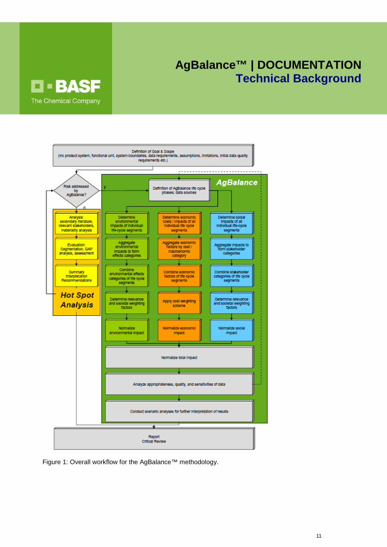
AgBalance™ studies follow specific and defined calculation methods (cf. Figure 1):

1) calculation of the total cost for the product system, and its impacts in terms of economic

sustainability,

2) a specific life cycle analysis for all investigated products or processes, according to ISO

14040 and 14044 standards,

1 Saling, P., A. Kicherer, B. Dittrich-Kraemer, R. Wittlinger, W. Zombik, I. Schmidt, W. Schrott, and S. Schmidt; Eco-efficiency Analysis by BASF: The Method; Int. J. Life Cycle Assess., 2002, 7 (4), 203. 2 Shonnard, D.; Kicherer, A; and Saling, P.; Industrial Applications Using BASF Eco-Efficiency Analysis: Perspectives on Green Engineering Principles; Environ. Sci. Technol. 2003, 37, 5340-5348. 3 Uhlman, B.; Saling, P.; Measuring and Communicating Sustainability through Eco-Efficiency Analysis, Chemical Engineering Progress 2010, 16, 17-26; available online 4 Kölsch, D; Saling, P.; Kicherer A.; Grosse-Sommer, A.; Schmidt, I.; Int. J. Sustainable Development, 2008, 11, 1, 1. 5 Schmidt, I., Meurer, M., Saling, P. Reuter, W., Kicherer, A. and Gensch C-O. ‘SEEBALANCE® managing sustainability of products and processes with the socio-eco-efficiency analysis by BASF, Greener Management International; 2005. 6 ISO, International Organization for Standardization. “Environmental Management -Life Cycle Assessment -Principles and Framework”, ISO 14040:2006, and “Environmental management –Life cycle assessment – Requirements and guidelines”, ISO 14044:2006, Geneva, Switzerland, www.iso.org.

9


3.) assessment of specific indicators relating to agricultural impact,

4) determination of social impacts for the product system,

5) calculation of relevance and calculation factors for specific weighting,

6) weighting of life cycle analysis factors with societal factors,

7) determination of the relative importance of environmental versus economic impacts as

well as social versus economic impacts

8) creation of fingerprint and single-score diagrams,

9) analyses of appropriateness, data quality, sensitivities, and scenario analysis, and

10.) investigation of additional sustainability impacts, which are not covered by the

AgBalance™ set of quantitative indicators, through a Hot-Spot Analysis.

A diagram showing the general workflow and elements of an AgBalance™ study is

presented in Figure 1.

1.5. Relationship of AgBalance™ to other reporting or assessment standards Developed by BASF, AgBalance™ is a methodology used to evaluate sustainability, based

on the principles of the Life Cycle Assessment framework, as defined in the ISO14040 and

14044 standards. However, it also defines a specific set of indicators and indicator

categories that relate exclusively to primary agricultural production.

In addition to these standards, AgBalance™ derives guidance from the following

certification and reporting standards or initiatives (see below).However, it is important to

clarify that AgBalance™ is not a certification or reporting standard for sustainable

agriculture. It is a methodology, which is designed to quantify and compare the performance

of agricultural solutions and products from a sustainability perspective.

UNEP-SETAC Guidelines for Social Life Cycle Assessment of Products: This is a general

methodology framework for integrating social aspects within the LCA concept. AgBalance™

references the SEEBALANCE® method for the social LCA, which covers the most important

aspects of the UNEP-SETAC guidelines, e.g., the concept of stakeholder categories.

10


ISO26000SR, and SA8000: These globally accepted standards for reporting and certifying

social sustainability within enterprises were considered during the development of

AgBalance™ agro-specific social indicators. AgBalance™ indicators are aligned with these

standards, e.g., categories ‘farmers/workers’ and ‘local/national community’.

11


Figure 1: Overall workflow for the AgBalance™ methodology.

12


ProSustainTM: Is a standard developed by DNV for product sustainability. BASF had already

developed the Sustainability, Eco-Efficiency, Traceability (S.E.T) program to help

companies and products meet the requirements of the ProSustainTM standard. The concept

of combining an LCA with the assessment of additional sustainability criteria as well as the

optional inclusion of a Hot Spot analysis have been adopted within AgBalance™.

ISCC (International Sustainability and Carbon Certification): BASF is a member of the ISCC.

ISCC is a certification system for renewable raw materials and defines a set of

environmental and social sustainability criteria, e.g., it implements good agricultural practice

and prohibits production in carbon-rich soils and high-value nature regions. In contrast,

AgBalance™ is designed to compare different product alternatives through comprehensive

analysis, where a holistic set of environmental, social and economic indicators are

quantified. Basic sustainability requirements, as set out by ISCC, can be used as principle

pre-conditions that alternatives have to fulfill or comply with (assuming a comparative

analysis with AgBalance™ has been initiated).

GRI (Global Reporting Initiative): BASF is an organizational stakeholder and reports,

according to GRI principles. For example, BASF’s 2011 report has been labeled A+ by GRI.

While GRI principles are focused on the reporting of corporate sustainability criteria, they

are not specific to agriculture. However, GRI Biodiversity indicators EN11-EN15 have

influenced the development of some indicators in the Biodiversity category of AgBalance™;

e.g., endangered species and protected areas.

WBCSD (World Business Council for Sustainable Development): BASF is member of

WBCSD. The ‘Guide to Corporate Eco-system Valuation’ provides guidance on how

corporations can evaluate their relationship with the eco-system and how they use eco-

system services such as clean water and air, renewable raw-materials. BASF sees

AgBalance™ as supporting the implementation of WBCSD-inspired principles.

13


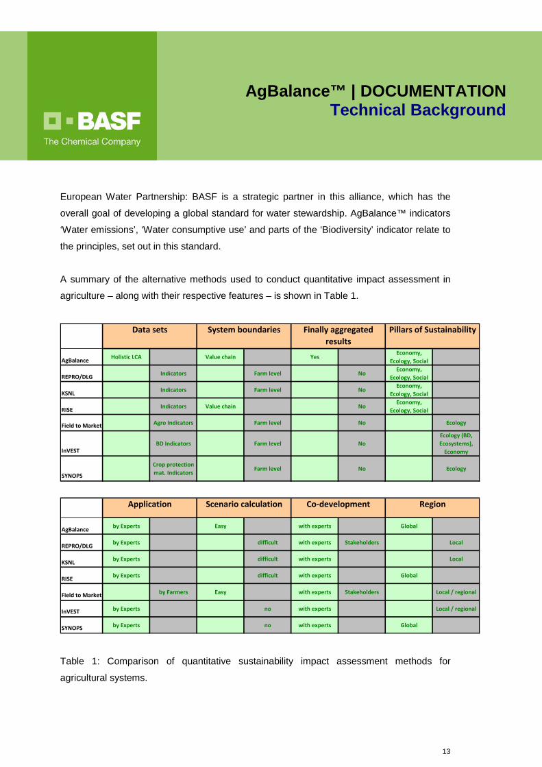
European Water Partnership: BASF is a strategic partner in this alliance, which has the

overall goal of developing a global standard for water stewardship. AgBalance™ indicators

‘Water emissions’, ‘Water consumptive use’ and parts of the ‘Biodiversity’ indicator relate to

the principles, set out in this standard.

A summary of the alternative methods used to conduct quantitative impact assessment in

agriculture – along with their respective features – is shown in Table 1.

Table 1: Comparison of quantitative sustainability impact assessment methods for

agricultural systems.

AgBalance Holistic LCA Value chain YesEconomy,

Ecology, Social

REPRO/DLG Indicators Farm level NoEconomy,

Ecology, Social

KSNL Indicators Farm level NoEconomy,

Ecology, Social

RISE Indicators Value chain NoEconomy,

Ecology, Social

Field to Market Agro Indicators Farm level No Ecology

InVESTBD Indicators Farm level No

Ecology (BD, Ecosystems),

Economy

SYNOPS

Crop protection mat. Indicators

Farm level No Ecology

AgBalance by Experts Easy with experts Global

REPRO/DLG by Experts difficult with experts Stakeholders Local

KSNL by Experts difficult with experts Local

RISE by Experts difficult with experts Global

Field to Market by Farmers Easy with experts Stakeholders Local / regional

InVEST by Experts no with experts Local / regional

SYNOPS by Experts no with experts Global

Data sets System boundaries Finally aggregated results

Pillars of Sustainability

Application Scenario calculation Co-development Region

14


2. Definition of Study Goals

The starting point for any AgBalance™ study is to determine the specific goals. This

provides the broader context and helps to define the target audience, the alternatives for the

study and the system boundaries. This definition of the study goals and context also helps to

identify the various points along the value-chain (in the life cycle), where sustainability

issues are the most prominent and hence have to be mirrored by the choice of system

boundaries). To this end, initial research should be conducted to record any economic,

environmental, and social aspects, associated with the process or product under

consideration. This can range from desk research to additional consultation with specific

institutions or data providers as well as potentially extending to wider involvement and

discussion with stakeholders, like NGOs, research institutes and authorities.

3. Functional Unit, Alternatives, and System Boundaries 3.1. Functional Unit / Customer Benefit

Based on the overall study goals, one can define the functional unit, i.e., the customer benefit

(CB) in AgBalance™7, the alternatives and the system boundaries.

The primary purpose of the functional unit/customer benefit is to provide a reference point for

the inputs and outputs of the product system. At a minimum, the functional unit/customer

benefit in the AgBalance™ model has to consider the location and the timeframe in which the

product is due to be provided, e.g., at the retail store, elevator or the farm gate or during a

particular growing season or average time period (e.g., 2007-2009) as well as the product’s

quality requirements (e.g., nutrient content). As defined by ISO the functional unit/customer

benefit has to be exactly the same for all compared product alternatives.

The definition of the customer benefit should consider customer needs (depending on the

study, this could be the farmer, consumer, retailer or agro-business). Typical examples for the

definition of the customer benefit are:

7 The term functional unit is used in the ISO standard. However, in AgBalance, the term ‘customer benefit’ is used. This is synonymous with functional unit.

15


- “Delivery of one ton of wheat grain to the mill, in the US middle-west. Quality of product is

to meet requirements for bread production, water content below x percent. Comparison

made on the basis of 2009 data.”

- “Production of one kg of packed cereal at a particular store. Quality requirements meet

standards set by retailer (protein content, carbohydrate content, energy content).

Comparison made on the basis of 2009 data.”

- “A three-year crop rotation of winter oil seed rape, using different types of grain (wheat,

barley, rye), that provides an energy quantity of x MJ. Products provided at the farm gate.

Comparison made on the basis of 2009 data.”

Any indicators that are quantified for the customer benefit are proportional to crop yield

(environmental and economy indicators) or to the working time needed to produce the

specified customer benefit (social indicators).

3.2. Alternatives

As AgBalance™ is a comparative analysis tool, it is important to include as many readily

available alternatives as possible for consideration. For each study, a minimum of two

alternatives has to be included. Different alternatives are defined by differences in the production systems (e.g., fertilizer

regime, pesticide regime), agricultural practice (no-till, conventional till, other differences in

machinery used), extensive/intensive production, irrigation, growing regions (with concurrent

differences in environmental, and socio-economic background), and the type of crop (e.g.,

sugar cane versus sugar beet, oil palm versus oilseed rape) and different crop rotations.

16


3.3. System Boundaries The scope of any AgBalance™ study is defined by its system boundaries. These boundaries

define the specific elements that are associated with raw material extraction, acquisition,

transportation, production, use, and disposal. It is important to remember that while

AgBalance™ considers the entire life cycle, it then concentrates on specific stages in the life

cycle where the alternatives under consideration differ. Any lifecycle stage that is identical for

every alternative under consideration can be excluded from the analysis as the same impact

applies across the board. However, any excluded factors must be examined to determine

whether inclusion would change the overall analysis result. When analyzing each alternative,

it is important to note that the same life cycle stages must be included. The system

boundaries are specifically defined for each AgBalance™ study, taking into account the CB

as well as the alternatives and guidance, provided by ISO 14040.

AgBalance™ may be used for both “product level” comparisons and “system level”

comparisons. Comparisons at the product level mean that different technologies or strategies

within a fixed system are compared, e.g., comparing different plant protection or fertilizer

regimes or tillage strategies under the same geographic and climatic conditions. On the other

hand, comparisons at the “system level” may address alternative systems that differ by crop

type as well as geographic/climatic zone, e.g., production of corn in an arid region as

compared with production systems in an area with a temperate climate.

3.4. Aspects of Geography, Time and Coverage of Value Chain for the Definition of

the Customer Benefit

In contrast with other agricultural impact assessment methods (e.g., FieldPrint Calculator,

RISE, REPRO), AgBalance™ does not impose limitations on either the geographical scope

or on the range of the value chain to be analyzed. The goal and scope can be adapted for

every case study. As a result, AgBalance™ offers great flexibility and can assess the

application of either very defined or relatively wide ranges of agricultural products and

processes.

17


The choice of geographical scope influences the level of data specificity and the data

sources, employed in the study. If an alternative is of national significance, statistical figures

from survey data can generally be used. If a particular growing region is under

consideration, data from regional institutions and associations can be used. If required, data

gaps can be filled through the use of surveys among farmers and other players in the value

chain.

4. Environmental Factors

4.1. Primary Energy Consumption (MJ/CB) This includes the cumulative energy used during the entire life cycle, including raw material

extraction, production, use and disposal as well as the energy content, remaining in the

products. All forms of energy are converted back to their primary energy sources, measured

in MJ/CB, including: crude oil, natural gas, coal, lignite, uranium ore, water power, biomass

and others. While the energy from biomass feedstock is included, the sun energy that is

needed to produce the biomass is excluded. The individual energy values are then summed

to arrive at the total primary energy consumption, required to fulfil the CB.

4.2. Raw Material Consumption (kg Silver Equivalents /CB) Key raw materials consumed are calculated for the entire life cycle in terms of kg/CB. Raw

materials are defined as the basic building blocks needed to create a product. At a minimum,

AgBalance™ will consider the following raw materials: coal, oil, gas, lignite, uranium, NaCl,

sulfur, phosphorus, iron, lime, bauxite, sand, copper and titanium.

Raw material consumption values are weighted with a factor that reflects the demand and

exploitable reserves of the raw materials, based on the statistical calculations of the U.S.

Geological Survey and other sources. Basically, the lower the reserves of a raw material

available and the higher the worldwide rate of consumption, the scarcer the material, and by

default, the higher the weighting factor assigned. These values are then transferred to an

18


easy understandable unit – expressed as silver equivalents which include energy-containing

components – as well as other types of abiotic resources. As a result, renewable resources,

which are assumed to have a sustainable management system in place and a theoretically

unlimited life span, yield a weighting factor equal to zero. A sustainable management system

includes certifications from institutions, such as The Forest Stewardship Council, The Wildlife

Habitat Council and The Sustainable Forestry Initiative. Renewable resources are considered

in the category of other environmental burden metrics and not in the category of raw material

consumption. In cases, where renewable raw materials are not managed in a sustainable

way (e.g., rainforest logging), the appropriate resource factor is applied.

4.3. Air emissions (kg/CB) Air emissions are calculated in terms of the mass of emissions, generated per CB (kg/CB)

over the entire life cycle. At a minimum, AgBalance™ considers but is not limited to the

following chemicals: CO2, SOX, NOX, CH4, non-methane volatile organic compounds (NM-

VOC), halogenated hydrocarbons (HC), NH3, N2O and HCl. These chemicals are then

grouped and the environmental burden reported under the following air emission categories:

− Global warming potential (GWP) - CO2, CH4, Halogenated organic compounds

(HCFC), N2O, weighted with IPCC factors8 and reported as CO2-equivalents.

− Photochemical ozone creation potential (POCP) - NM-VOC, CH4, reported as

ethene equivalents.

− Ozone depletion potential (ODP) - HC, reported as CFC-equivalents.

− Acidification potential (AP) - SOx, NOx, NH3, HCl, reported as SO2-equivalents.

The amount of air emissions is weighted by a factor, which reflects its potency in terms of

global warming, acidification, smog creation and ozone depletion potential. For example, air

emissions for each major greenhouse gas are adjusted for the 100-year GWP, as defined by

the Intergovernmental Panel on Climate Change (IPCC). 8

8 Forster, P., V. Ramaswamy, P. Artaxo, T. Berntsen, R. Betts, D.W. Fahey, J. Haywood, J. Lean, D.C. Lowe, G. Myhre, J.

19


Whenever significant inputs to the analysis are in biomass form, provisions are made to

account for land use change emissions, relating to CO2-equivalents.

4.4. Water Emissions (L/CB) Water emissions are assessed via a critical volumes approach, which considers both the total

amount of emissions released into water as well as the environmental impact of the

chemicals being emitted. The individual critical volumes are then totaled for a particular life

cycle stage in order to obtain an overall impact (L/CB). At a minimum, AgBalance™ will

consider the following quantities for water emissions: chemical oxygen demand (COD),

biological oxygen demand (BOD), N-total, NH4 as N, PO4 as P, absorbable organically bound

halogens (AOX), heavy metals, hydrocarbons (to include detergents and oils), sulfate and

chlorine. Sediments and particulates also have to be considered.

Critical volumes (CV) are calculated as a ratio of the amount of chemicals emitted, according

to the Maximum Emission Concentration (MEC) threshold limits. These are listed in the

annex to the German waste water ordinance. This methodology considers total water

discharge, including water emissions to both wastewater treatment systems and discharges

to surface waters. The greater the water hazard, posed by a substance, the lower its

discharge concentration limit. For example, an emission of 200 mg NH4-N with an MEC

threshold value 10 mg/L results in a critical volume of 20 L (CV = 200 mg/10 mg/L). There are

no provisions made to regionalize or localize the MEC values, used in the calculation, as it is

likely that these values are similar across different geographies (these are common

wastewater constituents with well-established toxicity levels). Regionalizing or localizing the

values would involve a great deal of effort and would not be likely to significantly improve the

accuracy of the results.

Nganga, R. Prinn, G. Raga, M. Schulz and R. Van Dorland, 2007: Changes in Atmospheric Constituents and in Radiative Forcing. In: Climate Change 2007: The Physical Science Basis. Contribution of Working Group I to the Fourth Assessment Report of the Intergovernmental Panel on Climate Change [Solomon, S., D. Qin, M. Manning, Z. Chen, M. Marquis, K.B. Averyt, M.Tignor and H.L. Miller (eds.)]. Cambridge University Press, Cambridge, United Kingdom and New York, NY, USA.

20


4.5. Solid Waste Emissions (kg/CB) In AgBalance™, the solid waste emissions account for all materials disposed of in a landfill.

Therefore, materials that are recycled or reused are not counted as solid waste. Waste is

categorized as municipal, hazardous, construction and mining with a weighting factor applied

to each type, relative to its potential impact. The weighting factors are 1, 5, 0.2, and 0.04 for

each waste category, respectively. These are subjective values, intended to reflect the degree

of potential environmental impact.

4.6. Eco-Toxicity (points/CB) In agricultural systems, chemicals are intentionally released into the environment, i.e.,

fertilizers and pesticides. As a result, eco-toxicity is integrated within the AgBalance™

methodology. Eco-toxicity potential is determined by the European Union Risk Ranking

System (EURAM).9 This is essentially a scoring system, which is based on the principles of

environmental risk assessment (i.e. risk as the product of hazard and exposure). Generally,

substances are ranked, based on their intrinsic properties, e.g., physicochemical and eco-

toxicological data and their ultimate end-point in the environment. This includes an

assessment of biodegradability, according to the OECD criteria (inherent/readily

biodegradable/persistent).

4.7. Land Use (m2a/CB – square meters times years per customer benefit The damage to ecosystems, resulting from land use in AgBalance™, is assessed, according

to the scheme developed by Koellner and Scholz.10,11 This is a formal model that includes

damage functions and generic characterization factors for quantifying damages to ecosystems

as a result of land occupation and land transformation. The characterization factor for land

occupation and land use change is labeled Ecosystem Damage Potential (EDP). A key feature

of this method is that land occupation and transformation is assessed, using a factual or

virtual restoration time period. This means that the land use damage is the most significant for

9 Saling, P.; Maisch, R.; Silvani, M.; König, N. Int. J. LCA, 10(5), 364-371 (2005) 10 Koellner, T., and Scholz, R., Assessment of Land Use Impacts on the Natural Environment, Part 1: An Analytical Framework for Pure Land Occupation and Land Use Change, International Journal LCA 12(1) 16-23, 2007. 11 Koellner, T., and Scholz, R., Assessment of Land Use Impacts on the Natural Environment, Part 2: Generic Characterization Factors for Local Species Diversity in Central Europe, International Journal LCA 2006

21


land use types that are difficult to restore and need extremely long time periods to recover

(e.g., over one thousand years for primary forest and peat bog).

Note on Indirect Land Use Change

At a minimum, an estimate of the GHG emissions resulting from ILUC should be made, using

the ‘top down approach’ and based on publications by WWF12 and Tipper et al.13 In this

method, the global GHG emissions, estimated to result from to land use change, are

attributed to commercial agricultural areas. This results in an averaged value of 1,42 tons of

CO2 equivalents per hectare of land, affected by indirect land use change.

4.8. Consumptive Water Use (points/CB) In AgBalance™, water use is assessed as a separate environmental impact category. The

method for assessing freshwater consumption, as described by Pfister, Köhler and Hellweg, is

used14. With this method, only consumptive water use is assessed. It should be stressed that

green water, which refers to precipitation and soil moisture consumed on-site by vegetation,

e.g., evapotranspiration, is not considered within AgBalance™. The employed method

includes regionalization and is based on GIS data as applied at the watershed levels. Details

of the corresponding regionalized damage factors are available in supplementary material

provided in the Pfister et alpublication at http://pubs.acs.org.

4.9. Biodiversity (dimensionless) General Remarks:

By definition, biodiversity cannot scientifically be quantified in its totality. Absolute figures are

highly variable. Some taxonomic classifications (species etc.) are not established, and the

functions and organisms depend on regional and local conditions. Therefore, any

quantification of “biodiversity” is an approximation, requiring the relevant elements of

biodiversity to be defined and the appropriate indicators used.

12 Audsley, E., Brander, M. Chatterton, J. Murphy-Bokern, D., Webster, C., and Williams, A. „How Low Can We Go? An Assessment of greenhouse Gas Emissions from the UK Food System and the Scope for Reduction by 2050“,WWF – UK 2009 13 Tipper, R.; Hutchinson, C.; Brander M, “A practical approach for policies to address GHG emissions from indirect land use change associated with biofuels”. Ecometrica, UK, 2009. 14 Pfister, S. Koehler, A. and Hellweg, S., Assessing the Environmental Impacts of Freshwater Consumption in LCA, Environmental Science & Technology Publication, American Chemical Society, April 23, 2009.

http://pubs.acs.org/

22


In AgBalance™, the impact of agricultural activity on biodiversity is assessed as a relative

function, constructed from the Biodiversity State Indicator and further indicators that have the

potential to increase or decrease biodiversity.

(1) Biodiversity State (state indicator) In AgBalance™, the vulnerability status of biodiversity in a particular region is assessed

by the number of endangered species published in the IUCN Red List for that region. 15

For Germany, the number of Red List species are assigned a biodiversity state of 0.7.

This definition is based on the published German national biodiversity index. Other

regions are assigned values through interpolation with zero endangered Red List

species, corresponding to a biodiversity state indicator of 1, and 4000 Red List species

to an indicator value of 0.1.

(2) Agri-Environmental Schemes (increase factor) Farmers may receive funding from Agri-Environment Schemes for services that promote

elements of biodiversity. Examples are flower strips (to support pollinators), pre-agreed

time of mowing (to improve the breeding success of meadow-inhabiting birds) or the

support of traditional farming practices. Programs include the Conservation Reserve

Program (US Department for Agriculture Farm Service Agency) and subsidies paid

under Pillar 2, Axis 2, of the EU Common Agricultural Policy agreement. Determining the

evaluation of the performance value (1.0 – 1.5) is specific for each study, according to

the following protocol. The lowest performance value of one (1.0) is assigned to zero

funding. The optimal performance value of 1.5 is given to the maximum attainable

funding in the countries or regions that are included in the specific study. Intermediate

values are then calculated from linear interpolation.

15 Wildlife in a changing world. IUCN, 2008; ISBN: 978-2-8317-1063-1

23


(3) Protected Areas (increase factor) The availability of protected (frequently but not always uncropped) zones is a very

important type of protection measure that promotes biodiversity in general. This

indicator measures any increases in protected area coverage.16 The indicator,

“Protected Area Coverage”, as defined and published by the Biodiversity Indicators

Partnership (BIP), is used.17 The protected area coverage (PAC) indicator is calculated,

using the designated national protected areas as recorded in the World Database of

Protected Areas (WDPA)18. The WDPA provides the most comprehensive, global and

spatial dataset on marine and terrestrial protected areas available. The data in the

WDPA is obtained from national and regional authorities as well as from non-

governmental organizations. The WDPA uses the IUCN definition of a Protected Area.

The evaluation of the performance value (1.0 – 1.5) is calculated using the following

protocol: the lowest value (1.0) is defined for 10 percent Protected Area Coverage (PAC)

and the highest value (1.5) for 30 percent PAC. Intermediate values are then calculated

from linear interpolation.

(4) Eco-toxicity (decrease factor) Plant protection products – including plant-incorporated protectants, such as GMO crop

varieties containing Bt-toxins for insect resistance – have the potential to influence

biodiversity. This potential is dependent on the product-specific ecotoxicity profile of

each compound, which are tested in laboratory, semi-field and field conditions for

registration purposes. Data for short-term (acute) and long-term (chronic) eco-toxicity of

plant protection products on earthworms, honey bees, rodents, birds, water fleas and

fish are therefore available from pesticide toxicity databases.19 Using the Initial Dose

concentration of the crop protection products, the LD50 values are determined by

dilution. The eco-toxicity potential of plant protection products is calculated by designing

16 Information retrieved from the Internet at www.bipindicators.net/pacoverage. 17 A detailed documentation of the indicator is published in Bubb, P. J., Fish, L. and Kapos, V. 2009. Coverage of Protected Areas –

Guidance for National and Regional Use. UNEP-WCMC, Cambridge, UK. 18 Available from: http://www.wdpa.org/ 19 http://ec.europa.eu/sanco_pesticides/public/index.cfm?event=activesubstance.detail

http://ec.europa.eu/sanco_pesticides/public/index.cfm?event=activesubstance.detail

24


the LD50 values of these products along a logarithmic scale with no dilution being

assigned the least worse value (1.0) and a dilution of 0,0001 assigned the worst score

(0.6). This process is followed for all crop protection products as well as for short and

long-term toxicity. The resulting ecotoxicity score is then multiplied by the amount of

crop protection product for each active ingredient, applied in g / ha / a. The final

ecotoxicity potential is calculated by adding the individual values for all crop protection

products. Finally, the indicator value is returned to the category scale within the

biodiversity indicator (0.6 – 1.0). This is achieved through a step-wise function, where

the best score (1.0) is assigned to alternatives having a low ecotoxicity potential and the

worst score (0.6) is assigned to the high ecotoxicity score.

(5) Farming intensity (decrease factor) Farming intensity, i.e. the intensity in the number and types of activities that occur in the

field as result of farming practices, such as plowing, mechanical treatment, fertilization,

crop protection etc., influence important elements in primary diversity, associated with

ecosystems. The trans-European study of Geiger et al.20 shows that there is a

significant correlation between biodiversity and yield. In AgBalance™, farming intensity

is therefore assessed indirectly as a function, located between the maximum attainable

yield and the actual yield of the alternative under study. Evaluating the performance of

this indicator is done by plotting the percentage of maximum attainable yield on a scale

from the worst score (0.6), relating to 100 percent of maximum attainable yield, to the

best score (1.0) for 20 percent of maximum attainable yield. A possible difference

between the maximum attainable yield and the actual yield has to be clearly linked to

measures that are promoting biodiversity, e.g., extensification.

20 Geiger, F. et al. Persistent negative effects of pesticides on biodiversity and biological control potential on European farmland.

Basic and Applied Ecology 11 (2010), 97-105.

25


(6) Nitrogen Surplus (decrease factor) Low rates of natural or synthetic fertilizer promote biodiversity since species-rich plant

societies are found in soils that are nitrogen-poor. Therefore, a nitrogen surplus is rated

as detrimental for biodiversity while AgBalance™ gives no credits for production

systems that are nitrogen depriving. The performance of this indicator is evaluated by

plotting the N-balance on a linear scale with the best score, (1.0) reached at minus 50

kg N/ha and the worst score (0.6) at a surplus of 150 kg N/ha.

(7) Potential for intermixing (decrease factor) The goal of this indicator is to assess the potential of specific crops to intermix with the

natural vegetation. Although the potential for outcrossing – coupled with the bewildering

range of modern crop varieties and their genes – is mostly discussed in relation to

genetically modified plants, all crop species have the potential to intermix with natural

vegetation. The intermixing potential is crop-specific and highly dependent on the

geographic region where the crop is grown (climatic conditions for growth and survival;

presence of pollinators and wild relatives). This indicator considers factors like the

potential for pollen dispersal through wind and insects, the availability of wild relatives,

the size of seed banks and seed persistence in soils as well as its adventitious presence

in machinery. A score is determined for each of these factors, ranging from worst (0.6)

to neutral (1.0) performance, based on a defined set of decision criteria. The final score

is the average of the individual scores.

(8) Crop Rotation (bidirectional factor) High crop rotation rates provide a diversity of plant-based resources that promote

biodiversity, such as root diversity (promoting soil organisms), flowers (promoting

pollinators), and foliage diversity (promoting plant feeding animals). From a biodiversity

perspective, the contribution of crop rotation can be summarized as follows: high rates

contribute to biodiversity increase and low rates to biodiversity decline. The evaluation

for this indicator is conducted on a linear scale for field crops. One element in crop

rotation commands the lowest score (0.6), three crops in a two-year rotation are

26


deemed as neutral (1.0) and seven elements in crop rotation within two years are

assigned the highest score (1.5). Crop rotation regimes may consist of several

elements, including intercropping of coverage or use of fertilization crops that promote

soil fertility.

4.10. Soil

General Remarks

The AgBalance™ methodology for the Soil impact category uses different indicators, which

are designed to capture the main impacts to long-term soil quality as a result of human

agricultural activity on arable landt. These indicators consist of: Soil Organic Matter balance,

Nutrients (N, P, K) balance, Soil Compaction Potential, and Erosion.

(1) Soil Organic Matter Balance (assessed kg carbon /ha) Organic soil matter is an important in determining soil quality as it influences the

chemical, physical and biological functioning of soils, especially in relation to the soil’s

capacity to store nutrients and water, its buffering and filtering capacity, its biodiversity

and structure. While it is obvious that a reduction in organic matter content will

eventually impair soil quality, the reverse is also true – high organic content is not a

positive development as this leads to high mineralization of nitrogenous compounds and

effluxes in the hydro- and atmosphere. The method used in AgBalance™ assesses

anticipates changes in the soil carbon balance due to cropping and allows the

opportunity for the soil to react to these influences, as published by Hülsbergen et al.21

The organic matter balance is a function of the influx of organic matter through organic

fertilizers (plant residues, manure, compost) and the crop specific change in organic

matter (due to type and intensity of soil preparations as well as the characteristic of its

root system). To identify the balance of organic matter, the degradation of organic

21 Küstermann, B., Kainz, M. & Hülsbergen, K. J. (2007): Modeling carbon cycles and estimation of greenhouse gas emissions from organic and conventional farming; Renewable Agriculture and Food Systems, 23 (2008), 38.

27


compounds is measured against the influx of degradable material. Soil organic matter is

quantified as organic carbon (C).

In AgBalance™, the carbon balance is calculated, using a computer model from the

Bavarian State Office for Agriculture (Bayerische Landesanstalt für Landwirtschaft). The

carbon balance result is subsequently evaluated, using a model designed by

Hülsbergen et al. Effectively, a carbon balance between minus 100 kg C/ha and plus

200 kg C/ha is rated optimal (1.0) with scores decreasing in a linear fashion for lower or

higher carbon balances.

(2) Nutrients Balance (assessed kg nutrient / ha) Assuming the ecological impacts of over-fertilization, the input of fertilization should be

optimized, according to both the crop’s requirements and the nutrient status of the soil.

This approach ensures an appropriate supply of nutrients for crops. The nutrient

balance is therefore a function of the amount of fertilizer applied and the amount of

nutrients retrieved through the harvesting of the crop. This balance is further adjusted to

factor in the the ability of the soil to mineralize and provide nutrients, as indicated by soil

nutrient supply classes. The nitrogen balance considers different sources e.g., nitrogen

fixation by leguminous crops. The result of the nutrient balances is subsequently

evaluated, using nutrient- specific models with optimal scores (1.0), approximately

equating to an equal nutrient balance of zero and with decreasing scores for either

nutrient deprivation or over-fertilization.

(3) Potential for Soil Compaction (performance score) Soil compaction refers to the deterioration of soil structure (the loss of soil features) due

to mechanical pressure, predominantly from agricultural practices. The method for

assessing soil compaction in AgBalance™ has been devised by Dr. Paul Newell-Price et

28


al. at ADAS UK Ltd.22 The aim of the method is to produce a simple empirical

relationship that allows the soil compaction risk to be assessed, either at field, farm or

regional level, taking into account any parameters/factors that have an influence on soil

compaction. These factors can be related to the nature of the soil being assessed, using

the Harmonized World Soil Database23, climate as well as considering the way the soil

is being managed. The individual evaluation factors are given a numerical score of 1

(low risk for compaction) to 3 (high risk). The overall risk for soil compaction is evaluated

by a multiplication of all factors. The resulting indicator value for each alternative is

normalized to the worst alternative. This normalized result is subsequently used as a

parameter in the calculation of the soil index.

(4) Soil Erosion (t/ha/a) In AgBalance™, soil erosion caused by runoff is calculated, using the Universal Soil

Loss Equation (USLE). This equation predicts the long term average annual rate of

erosion in a field, based on slope, rainfall pattern, soil type, topography, crop system,

and management practices. USLE only predicts the amount of soil loss that results from

sheet or rill erosion on a slope and does not take into account additional soil losses that

might occur from gully, wind or tillage erosion. Where these effects have a significant

impact, they are factored in by appropriate modeling, e.g., wind erosion through

estimates by the Revised Wind Erosion Equation. In addition, alternative management

and crop systems can be evaluated to determine the adequacy of conservation

measures in farm planning.24 In AgBalance™, the absolute calculated soil loss –

resulting from the USLE calculation for each alternative – is used to relatively compare

alternatives with the normalized result. This normalized result is subsequently used as a

parameter in the calculation of the soil index.

22 Assessment of Soil Compaction Risk (Project Report), Paul Newell-Price, ADAS UK Ltd., 2011 23 FAO/IIASA/ISRIC/ISSCAS/JRC, 2009. Harmonized World Soil Database (version 1.1). FAO, Rome, Italy and IIASA, Laxenburg, Austria. Internet: http://www.iiasa.ac.at/Research/LUC/External-World-soil-database/HTML/ 24 http://www.omafra.gov.on.ca/english/engineer/facts/00-001.htm 7.02.2011

29


5. Economic Factors

5.1. Consideration of costs

AgBalance™ methodology aims to assess the economics associated with products or

processes over their entire life cycle and determine an overall total cost of ownership for the

customer benefit (€/CB). The approach for calculating costs varies from study to study. When

agricultural products for the consumer are being compared, the sale price paid by the

customer is used. When different production methods are compared, the relevant costs

include the purchase and installation of capital equipment, depreciation and operating costs.

The costs incurred are summed and combined in appropriate units (e.g., dollar or euro)

without weighting individual financial amounts. Regardless of the method used, the

AgBalance™ methodology incorporates:

the real costs that occur during the process of creating and delivering the product to

the consumer;

the subsequent costs that may occur in the future (due to tax policy changes, for

example); and

the costs associated with ecology, such as the costs involved in treating wastewater,

generated during the manufacturing process.

In AgBalance™, costs are quantified for each alternative, according to the metrics specified

below. They are then aggregated and totaled to show the total cost of each alternative as it

relates to the common customer benefit.

5.2. Consideration of indicators of economic sustainability

The main purpose of these indicators is to assess the economical sustainability of agriculture

at a segment or national level as well as for international comparisons.

30


It is important to note that the variable and fixed cost metrics, specified above, are quantified

in relation to the customer benefit (functional unit). In contrast, the macroeconomic indicators

are quantified per unit of area (e.g., hectare). The reason for this approach is that costs like

emissions in the environmental assessment can be related in a meaningful way to certain

production volumes for a specific crop. However, this is not the case for economic figures,

like profits or subsidies. For example, increasing the yield per hectare might result in a higher

profit per hectare and higher farm business profits, but not necessarily in a higher profit per

ton of product. However, for the farm business as a whole, the former is the most important

(i.e., the higher profit per hectare), and not the profit per ton of product. The results of the

macroeconomic indicators relate to a defined unit, e.g., hectare. They are also aggregated

and totaled for each alternative.

5.3. Aggregation of costs and macro-economic indicators To calculate the final economic score, the resulting values are then normalized to the worst

alternative and are subsequently aggregated by a weighting scheme.The weighting scheme

for the aggregation of economic categories is defined as follows:

Total costs = sum of variable costs and fixed costs

Economic score = 0,50 (normalized total costs)

+ 0,50 (normalized macroeconomic indicators)

5.4. Time and regional aspects of costs Cost analysis in AgBalance™ can be calculated at either a single point in time or alternatively

over a period of time that takes into account the time value of money. If the analysis is

performed to account for the time value of money, then a Net Present Value or similar metric

is calculated to correspond with the time frame of the cash flow and the assumed discount

rate specified. In international comparisons, the local currency is converted to US dollars,

according to purchasing power parity considerations. This transformation takes into account

not only the exchange rate but also the money needed to buy a certain basket of goods in a

31


given country. This means that the transformed wages can be compared directly across

different countries.

5.5. Economic Cost Metrics The exact metrics chosen for a study depend upon the CB, the alternatives, the system

boundaries with due consideration of the elements, described in Section 2. Each economic

metric, included in the AgBalance™ study, must be consistently applied to each alternative

and cover all relevant costs, including revenue, where applicable. At a minimum, it includes

consideration of the following (where appropriate):

Raw material

Labor

Energy (electric, steam, natural gas, and other fuels)

Capital investment

Maintenance

EH&S programs and regulatory costs

Illness and injury costs (medical, legal, lost time)

Property protection and warehousing costs

Waste costs (hazardous; non-hazardous)

Transportation

Training costs

Others, as applicable (e.g., taxes, levies)

For the life cycle module of the Farming Step, several specific costs, associated with

agricultural production, have to be considered. The AgBalance™ methodology will

incorporate (but is not restricted to) the following economic metrics, specific for agricultural

activities:

Variable costs

(1) Costs for soil preparation

32


(2) Costs for seed and sowing

(3) Costs for crop protection

(4) Costs for harvest

(5) Costs for drying

(6) Costs for machinery Fixed costs

(7) Depreciation

(8) Maintenance costs

(9) Insurance

(10) General repair cost

(11) Investment

(12) Employees

5.6. Macro-economic indicators

For each alternative, the macro-economic indicators are quantified, according to the

principles outlined below. The resulting values, expressed in monetary value per

hectare, are then summed, according to the formula:

Macro-economic Indicator Result (a) [USD/ha]

= Farm Profits (a) [USD/ha] – Subsidies (a) [USD/ha] + Productivity (a) [USD/ha].

Here (a) denotes the specific result for a given alternative. The macro-economic indicator

value is then aggregated with the costs in order to calculate the economic score for

each alternative.

(1) Subsidies (monetary value per unit of area) Negative - lower are seen to be better

33


As subsidies make up a large percentage of farm income in many countries, this aspect

is taken into account. The definition of subsidies in this instance includes all direct

payments to the farmers by national or supranational authorities, excluding those paid

for agri-environmental schemes. However, subsidies per se, have a distorting effect on

the national and international economy and create uncertainty for the farmer in the mid-

to long-term. Economists also argue that subsidies for agricultural production over the

long-term result in increases in the cost of leasing land.

(2) Productivity (monetary per unit of area) Positive - higher numbers are seen to be better. The indicator is defined as the (i) the absolute contribution that production makes for

each alternative to the national agricultural gross domestic product (GDP) per unit of

area (ii) weighted by what agricultural GDP contributes to the total national GDP,

expressed as a percentage. By combining these two features, each alternative’s

economic contribution to the societal role of agriculture is duly quantified. In cases

where agriculture makes up a larger percentage of total GDP, the second factor can be

viewed as a characterization factor that gives agricultural GDP per area a higher impact

(3) Farm Profits (monetary value per unit of area) Positive - higher numbers are seen to be better) This metric is an important economic indicator of profitability. Profitability is closely

related to sustainability as sustained economic activity ultimately drives environmental

and social responsibility. Profits are quantified per unit of area (e.g., hectare) since

economic figures related to profitability, like profits or subsidies, cannot be meaningfully

related to a certain crop production volume. For example, increasing the yield per

hectare might result in a higher profit per hectare and higher farm business profits but

not necessarily in a higher profit per ton of product. Also, crop yield is not the only driver

of profits. For example, extensive organic farming may have substantially lower yields

34


than conventional farming but can nonetheless deliver high profits through higher sales

prices.

35


6. ™Social Factors

Social parameters are not addressed specifically in the ISO LCA standards. There are no

other consensus standards that can be referenced to define the criteria for a social LCA.

AgBalance™ represents BASF’s best attempts to create a social LCA framework through the

identification and use of relevant factors associated with life cycle principles. Even though

there are no industry standards available, important developments from different groups like

the UNEP/SETAC working group or existing standards in the Agro-sector like RISE were

considered.

The social assessment in AgBalance™ is built on the SEEBALANCE® scheme for social LCA,

which was developed in 2005 by the Universities of Karlsruhe and Jena, the Öko-Institut

(Institute for Applied Ecology) Freiburg e.V., and BASF respectively.4,5 During this

development process, concrete targets for social sustainability for products and processes

were derived. This was done through analysis of more than 60 published studies on the topic

of social goals by various institutions. As a result, more than 700 goals and more than 3,200

indicators were systematically recorded, categorized and summarized.

For AgBalance™, this set of social parameters has been extended and in parts modified, to

address specific agricultural sustainability topics, e.g., access to land, level of organization or

international trade with agricultural products. These topics were initially identified through a

stakeholder process in 2009 and 2010, organized by BASF, and were subsequently

discussed with leading experts. Feedback from this process was then integrated into the

development of these indicators.

Social factors as part of AgBalance™ means integrating social parameters into the

assessment model, taking all three pillars of sustainability into account, as originally proposed

in the definition of sustainability by the UN Brundtland commission. The strength of a life cycle

approach is that social aspects along the life cycle, e.g., the considered value chain of a

product are tracked and any problems associated with shifting from one life cycle stage to

another is avoided. The assessment of social indicators shows the sustainability risks or

36


weaknesses, as well as strengths of any given alternative. It is worth noting that any

alternatives that reflect conditions conflicting with legal rights or basic human rights will not be

assessed in an AgBalance™ study.

In the specific case of child labor, an assessment of an alternative, i.e., comparing an

agricultural process with child labor versus a process without child labor will not be subjected

to comparative analysis within AgBalance™. However, child labor might occur in upstream

processes, e.g., mining of raw materials that are part of the pre-chain of many manufactured

goods. In such a case AgBalance™ can address and quantify this sensitive aspect in order to

be transparent and comprehensive on the life cycle of a product system,

6.1. Social Factors for Up- and Downstream Processes The assessment of social impacts in the upstream and downstream processes within

AgBalance™ is based on the SEEBALANCE® method. This approach to social assessment

is based on a sectoral approach where key social figures from different industry segments

are related to their corresponding production volumes. The resulting social profiles for

processes or products then assume a format, equivalent to the eco-profiles in the

environmental section.

For all social indicators, the production volumes are related quantitatively to a given industry

sector (e.g., ‘occupational diseases per kg product’). With this approach, it is possible to

relate the inputs and outputs from the environmental life cycle assessment to the individual

social indicators. To this end, different statistical databases are combined to connect social

indicators to production volumes. The link between products and corresponding social

impacts is made by a sector assessment. This is based on either the ‘Nomenclature générale

des activités économiques dans les Communautés Européennes’ (NACE, general

nomenclature of economic activities in the European Community) – an initiative that

classifies all industries into different sectors – or the ISIC, the International Standard

Industrial Classification. All products can be linked to these NACE/ISIC codes, using the

37


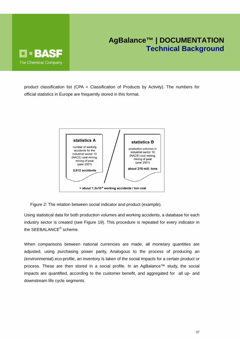
product classification list (CPA = Classification of Products by Activity). The numbers for

official statistics in Europe are frequently stored in this format.

Figure 2: The relation between social indicator and product (example). Using statistical data for both production volumes and working accidents, a database for each

industry sector is created (see Figure 19). This procedure is repeated for every indicator in

the SEEBALANCE® scheme.

When comparisons between national currencies are made, all monetary quantities are

adjusted, using purchasing power parity, Analogous to the process of producing an

(environmental) eco-profile, an inventory is taken of the social impacts for a certain product or

process. These are then stored in a social profile. In an AgBalance™ study, the social

impacts are quantified, according to the customer benefit, and aggregated for all up- and

downstream life cycle segments.

38


6.1.1. Stakeholder Category Employees

(1) Working accidents and fatal working accidents (number per CB)

Negative – lower numbers are seen to be better.

The definition of this indicator evaluates the potential of working accidents: Events are

considered as working accidents if the affected staff members are unable to work for

more than three days. The number of working accidents is recorded in association with

an activity (production). The numbers are expressed as the numbers of accidents or

fatal accidents.

(2) Occupational diseases (number per CB)


Occupational diseases are illnesses that can be definitively attributed to occupational

activity. The number of occupational disease is recorded in association with an activity

(production). The numbers are expressed as the number of occupational disease cases.

(3) Human toxicity (toxicity score per CB)


The assessment of human toxicity potential is not based on statistical figures but rather

on a calculation scheme for chemical substance, described below. The toxicity potential

is assessed not only for the final products but also for the entire pre-chain of chemicals,

used to manufacture the products. An inventory of the quantities of each substance,

included in the analysis, must be maintained in order to calculate overall toxicity

potential. The result is an assessment of life cycle toxicity potential that includes not only

the final products but also the reactants required in its manufacture. In addition, the

toxicity potential is also quantified for the use and disposal stages of the life cycle. The

general framework for performing the analysis of toxicity potential is described by

39


Landsiedel and Saling25 and is based upon the Hazardous Materials Regulations (R-

phrases), as outlined in Directive 67/546/EEC. This method was chosen because in

order to score the toxicity of a substance, the consideration of all possible effects is

needed. The R-phrase system is widely used in Europe for the classification of a

substance's various toxic effects. With the introduction of the Globally Harmonized

System (GHS) for the classification of hazards, the existing scheme adapts to the new

classification by mapping the R-phrases to the new system categories.

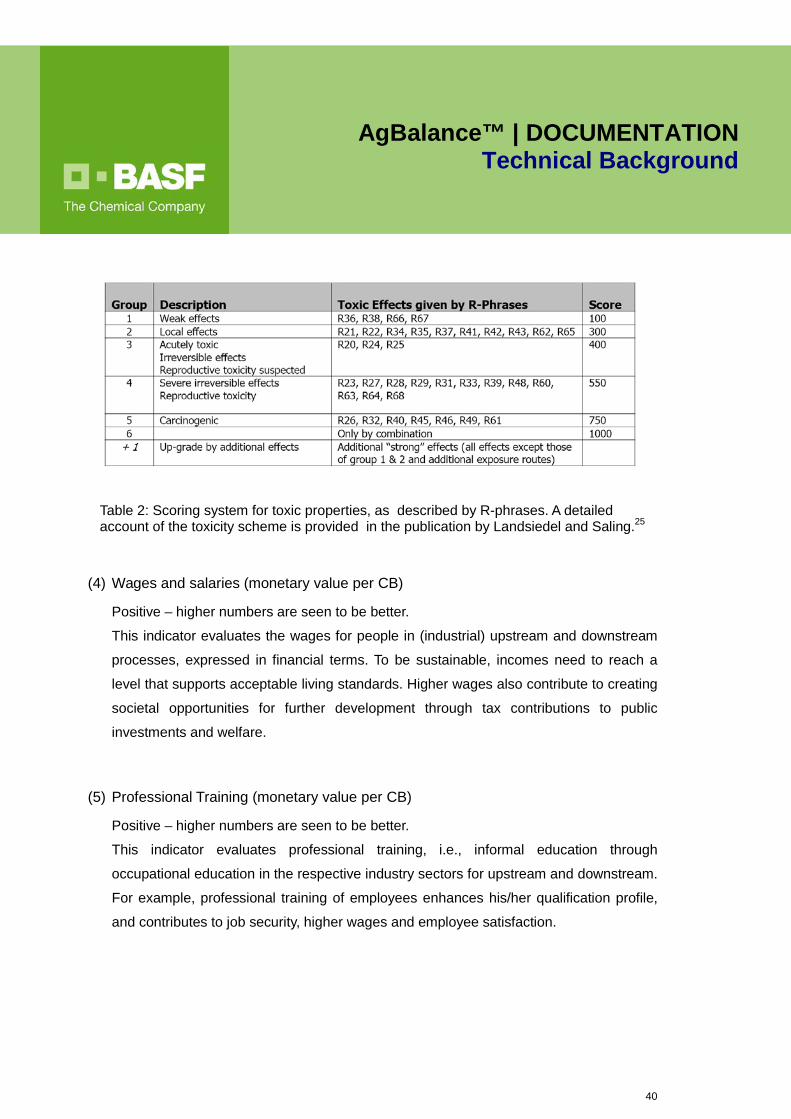
For AgBalance™, the toxicity potential assessment focuses on human toxicity potential.

The scoring system (Figure 3) is based on six groups of toxic properties, described as

R-phrases. Each group is given a score, ranging from 100 to 1,000, based on the

severity of the toxic effects. A substance is assigned to one of these groups on the basis

of its toxic properties, also described as R-phrases. If there is only one R-phrase for the

substance, it will be assigned to the appropriate group. However, if there are additional

R-phrases, the substance will be upgraded. However, weak effects or local effects

(group 1 and group 2 respectively) or alternatively, the same effect, caused by an

additional exposure route (e.g., oral and dermal), will not lead to an upgrade. In general,

there is only one upgrade for a substance, irrespective of how many additional R-

phrases are present. Scoring for toxicity, based on R-phrases, is conducted, according

to the following scheme. Refer to Table 2.

25 Landsiedel, R.; Saling, P. Assessment of Toxicological Risks for Life Cycle Assessment and Eco-efficiency Analysis. Int. J. Life Cycle Assess. 2002, 7 (5), 261-268

40


Table 2: Scoring system for toxic properties, as described by R-phrases. A detailed account of the toxicity scheme is provided in the publication by Landsiedel and Saling.25

(4) Wages and salaries (monetary value per CB)

Positive – higher numbers are seen to be better.

This indicator evaluates the wages for people in (industrial) upstream and downstream

processes, expressed in financial terms. To be sustainable, incomes need to reach a

level that supports acceptable living standards. Higher wages also contribute to creating

societal opportunities for further development through tax contributions to public

investments and welfare.

(5) Professional Training (monetary value per CB)


This indicator evaluates professional training, i.e., informal education through

occupational education in the respective industry sectors for upstream and downstream.

For example, professional training of employees enhances his/her qualification profile,

and contributes to job security, higher wages and employee satisfaction.

41


(6) Strikes and lockouts (lost working hours per CB)


Freedom to assemble and a guarantee of human rights are assumed to be

preconditions that must be fulfilled. Otherwise, this topic would be critically assessed as

a hot spot and might mean that a comparative AgBalance™ study would not be

appropriate (kill criterion). Taking this as a basic criterion, the indicator highlights

working conditions and the recognition of employee interests.

6.1.2. Stakeholder Category Consumer

(1) Human toxicity (toxicity score per CB)


This indicator evaluates potential human health impacts on customers. The assessment

takes into account the toxicity potential of materials that are part of the studied system

as well as a simple estimate of the exposure risk (toxicity points during use, exposure,

and vapor pressure), using the methodology described above in Section 6.1.1.(3).

These factors are combined into a performance rating, expressed in ‘toxicity points’.

This indicator is used to assess any toxicity risks that particularly affect the end-

consumer.

(2) Functional product characteristics (normalized performance per CB)


Additional, relevant product characteristics – which are not considered in any of the

other indicators – can be rated here. The indicator must be specifically defined,

depending on the product and its requirements. It is evaluated on the basis of technical

requirements being fulfilled with subsequent normalization or in some cases with ABC

analyses. For example, fuels for combustion engines must fulfill the requirements for

purity and viscosity for use at cold temperatures. This might be a differentiating feature

for biodiesel versus conventional fuels. These types of technical requirements and the

42


extent to which they are realized must be considered if one is to arrive at meaningful

and balanced results.

(3) Other risks (normalized performance per CB)


This indicator evaluates the potential risks to human health for any consumers that fall

outside the toxicity assessment. The assessment takes into account product

characteristics like explosiveness or corrosiveness etc. This indicator particularly

assesses any risks that do not arise from farming activities but from upstream and

downstream processes.

6.1.3. Stakeholder Category Local and national community

(1) Employment (working years per CB)


This indicator evaluates the number of working hours associated with the production

system for the upstream and downstream processes. It specifically measures the

contribution that the product system makes to employment and job creation.

(2) Qualified employees (working years per CB)


This indicator calculates the working time that qualified employees with a formal degree

dedicate to a specific product system versus unskilled worker. A higher level of

qualification is associated with improved social status for the employee. Typical benefits

include better job security, salary and work satisfaction.

(3) Gender Equality (working years per CB)


43


In the assessment of upstream and downstream industrial production steps, this

indicator is calculated by referencing the number of female managers (higher level) in

the respective industry sectors. In general, gender discrimination limits the potential of

families, communities and societies. There is a clear, positive link between gender

equality and economic and social development.

(4) Integration of disabled employees (working years per CB)


This indicator assesses the employment rate for people with severe disabilities in

upstream and downstream processes that are part of the product system. Results are

expressed as the number of disabled people employed. Integrating people with

disabilities into employment is commonly perceived as an indicator of societal

development. As major employers in the world economy, it is important that agricultural

and food chain businesses offers employment opportunities for all members of society.

(5) Part time workers (working years per CB)


This indicator calculates the proportion of part-time workers with reduced working hours

in comparison to full-time employees in the upstream and downstream processes,

associated with the product system. In this instance, part-time work is viewed positively

as it offers workers flexibility in managing their working and personal lives. This is

associated with higher levels of satisfaction and well-being

(6) Family support (monetary value per CB)


This indicator evaluates – in financial terms – the impact of parental leave and other

bonuses offered to employees, who are married and/or have children, including health

44


insurance and support for births, deaths etc. The indicator is included to reflect the

support that employees receive for family issues. It measures how institutions and

employers value the important role that families play in society.

6.1.4. Stakeholder Category International community

(1) Child labor (working hours per CB)


As discussed above, child labor is not included in the assessment of agricultural

production activities. In short, the customer benefit definition and the definition of

alternatives are not designed to assess child labor. However, child labor may still occur

in upstream processes, e.g., mining of raw materials that form part of the pre-chain of

many manufactured goods. AgBalance™ can address and quantify this sensitive

aspect, ensuring visibility and tracking within the life cycle of a product system. Different

regions are not excluded from studies as they may be important when considering

complete markets and market shares for produced goods. This is important as a basic

condition for AgBalance™. It also helps to identify improvement potential for alternatives

that are linked with child labor.

(2) Foreign direct investment (monetary value per CB)


The definition of this indicator is foreign direct investment in developing countries from

the perspective of the country under study Investment in developing countries

contributes to that country’s economic development through the creation of job

opportunities either directly or indirectly through demand for manufactured goods.

(3) Imports from developing countries (monetary value per CB)


45


This indicator rates the monetary value associated with the import of raw-materials,

industrial goods etc., that are part of the product system for upstream and downstream

processes. This specifically relates to situations where goods from developing countries

are imported into well-developed countries, resulting in a net amount of money moving

from the higher-income to the lower-income region. As it contributes to the income of

local producers, it also supports the economy in the developing region.

6.1.5. Stakeholder Category Future generations

(1) Number of trainees (number of persons per CB)


This indicator assesses the number of people in formal education within the industrial

sectors, associated with the relevant upstream and downstream processes. In order to

meet future economic challenges, it is a key societal responsibility to educate future

generations to a high standard.

(2) R&D expenditures (monetary value per CB)


This indicator quantifies the internal and external expenditure of companies in R&D

activities. R&D Investment in is seen to positively influence the future development of

manufacturing industries. As such, it helps to maintain good, current working conditions

as well as sustaining future job opportunities

(3) Capital investment (monetary value per CB)


This definition covers the value of replacement and net investment, including general

repair, purchase of concessions, patents and licenses (capital investment in € per

product masses). A higher rate of investment indicates that the companies associated

with the product system enjoy a positive economic situation that allows them to invest.

46


This is an important criterion for sustained economic activity, which supports an

improvement in both existing and future working opportunities.

(4) Social security (monetary value per CB)


This assessment summarizes the payments employers make to health insurance

schemes and unemployment insurance, pensions and similar programs for their

employees. The evaluation is done by each individual industry sector and relates to

upstream and downstream processes that are part of the product system.

6.2. Social Factors for the Farming Module The goal of these social, indicators is to quantify the relevant social impacts, described

above, for the agricultural steps in the life cycle. The required degree of detail does not allow

the use of general statistical data for the agriculture sector. Instead, specific data has to be

generated and assessed for each indicator, using specific data-sources and algorithms.

These indicators are designed to closely match the social sustainability areas, addressed in

the assessment of the upstream and downstream processes. Some indicators are specific for

the Agro sector, i.e., access to land and the degree of organization by farmers.

6.2.1. Stakeholder Category Farmer

(1) Wages (monetary value per CB) Positive – higher numbers are seen to be better.

The wages of agricultural workers are taken as a criterion for working conditions. They

contribute to (i) the material welfare/well-being of employees and (ii) the attractiveness

of agriculture as a sector.

The indicator is calculated as a function of the wages and the number of working hours,

needed to produce the customer benefit.

47


(2) Professional Training (ratio, training hours per working hours), Positive- higher ratio is seen to be better. Professional training benefits the individual farmer/employee as well as the overall farm

operation. After all, the individual needs qualifications to ensure continued success and

satisfaction in his/her job. Generally, qualified workers are required to ensure the

economic success of the farm and to guarantee that proper practices are implemented.

Professional Training is defined as non-formal, occupational education, associated with

agriculture. This indicator is calculated as the ratio between the working hours spent on

professional training relative to the total working hours.

(3) Association memberships (ratio, number of memberships and associations per farmer) Positive – higher ratio is seen to be better.

Membership of agricultural associations, unions and other organizations is seen to be a

positive development as it supports and enhances (i) the individual interests of farmers/

employees, (ii) raises public awareness and acceptance of agriculture (iii) increases

consumer confidence in agricultural products.

This indicator is calculated by taking the average of the ratio between the membership

subscriptions for any agricultural organization as it relates to the total number of workers

in the region and sector, as well as the number of all associations, organizations, etc.

that serve farmer interests in the region and sector under analysis. This is then divided

by the total number of workers in the region and sector.

6.2.2. Stakeholder Category Consumer

(1) Residues in feed and food (performance rating, percentage maximum residue level exceedance) Negative – lower numbers are seen to be better)

The indicator assesses the percentage of food samples that exceed official maximum

residue limits (MRLs). The indicator is based on a retrospective analysis of MRL

48


exceedances in food products, based on food monitoring reports by authorities. It is

aimed at ensuring consumer safety and confidence.

This indicator assesses the number of exceedances in a defined region over a specific

time period (typically a year), using a linear function that takes a value of one, if the

exceedances are zero, and a value of 100 if exceedences are measured as nine

percent of the samples (as defined by expert judgement to be a worst case scenario).

However, there is no upper limit.

(2) Presence of unauthorized/unlabeled GMO in feed and food (performance rating, number of occurrences), Negative – lower numbers are seen to be better.

This indicator is based on a retrospective analysis of reported occurances of unlabeled

or unauthorized residues of genetically modified organisms (GMO) in food products

(based on official food monitoring reports). The indicator is aimed at consumer

confidence.

This indicator assesses the number of reported occurrences of unauthorized or

unlabelled GMO material, found in food samples in a defined region over a 10-year time

period. The number of occurrences is indexed, using regression in time, i.e., one

occurrence in the year of assessment is scored as one, whereas one occurrence five

years before is scored as 1/5. The final score is the summary over 10 years.

6.2.3. Stakeholder Category Local & National Community

(1) Land owner/access (monetary value per CB) Negative – lower numbers are seen to be better.

Continued and reliable access to land is important for a farmer to plan his operations

over the mid-term. In the long-term, it is a prerequisite for investment. A dependency on

49


leased land means risk in terms of land availability and associated costs. Land lease

prices are rising globally due to several factors, including property speculation.

This indicator therefore calculates the percentage of leased land – within the agricultural

area – that is used for the benefit of the customer, multiplied by the cost of the lease.

For countries covered by the International Fund for Agricultural Development of the

United Nations (IFAD), a performance ranking for “Access to Land” (equitable access to

productive natural resources and technology) is available26. In AgBalance™, the use of

the IFAD indicator system is an alternative approach in studies where (i) the indicator

system is available for all countries considered and (ii) discussions with stakeholders

and experts have led to the conclusion that the use of the alternative approach is more

appropriate, e.g., a well-developed market for land does not exist.

(2) Employment (working hours per CB) Positive – higher numbers are seen to be better.

Higher employment rates and good employment opportunities are generally regarded as

positive for the local, rural community and society as a whole.

This indicator therefore calculates the number of working hours – associated with the

production system – per customer benefit.

(3) Gender equality (deviation from target value) Negative –lower numbers are seen to be better.

Discrimination by gender limits the potential of families, communities and societies in

general. For example, the importance of gender to the agricultural sector was recently

highlighted in a comprehensive report, published by the FAO27. There is a clear, positive

link between gender equality and economic and social development.

26 http://www.ifad.org/gbdocs/gc.htm 27 Gender dimensions of agricultural and rural employment: Differentiated pathways out of poverty, FAO 2010, ISBN 978-92-5-106583-9

50


In this indicator, the percentage of women who are farm proprietors or farm managers is

assessed in relation to the overall percentage of the female population in society.

Deviations to both higher and lower values are rated negatively. However, the analyst

generally evaluates which are the major barriers that women have to overcome in order

to achieve gender equality. If necessary, the exact definition of the indicator can be

adapted to suit study-specific needs, taking the overall context into account (regional,

cultural, economic).

(4) Integration of Disabled Employees (working hours per CB) Positive – higher numbers are seen to be better.

Apart from discrimination by race, religion or gender, people with (severe) disabilities are

frequently subject to discrimination in labor relations. This fact has been emphasized by

ILO and in the ISO26000 Social Responsibility Report.28 This indicator takes into

consideration the employment of people with (severe) disabilities relative to the total

working hours in the agricultural sector, per customer benefit.

6.2.4. Stakeholder Category International Community

(1) Developing countries import / trade balance (monetary value per year) Positive – higher numbers are seen to be better.

In developing countries, agriculture often contributes to a large percentage of GDP. One

strategy is to raise the income of local farmers by exporting produce to other countries.

However, the import of agricultural/food products from well-developed countries into

developing countries often puts local producers under pressure as they have to

compete with the (potentially low) prices of the imported goods.

This indicator rates the import and export value of the good(s) under analysis (e.g.,

potatoes) as it contributes to the trade between higher and lower income countries. In

AgBalance™, the UN Human Development Index of per capita income is used to define 28 ISO26000SR, Guidance on Social Responsibility, International Organization for Standardization, 2010.

51


how trading countries are ranked with the FAO TRADESTAT database seen as a major

data source of import/export values for various agricultural products. A positive trade

balance for the country with lower per capita income is favored.

(2) Fair trade benefits (monetary value per CB) Positive – higher numbers are seen to be better.

Producer prices are an important criterion for the social sustainability of agricultural

production, especially for small farmers in developing countries. The goal is to compare

the producer prices for different alternatives to producer prices on the free market, as

provided by the UN Food and Agriculture Organisations database FAOSTAT.29, Benefits

and premiums, obtained through the Fair Trade program and certified by the Fair Trade

Labelling Organizations International (FLO, www.fairtrade.net) are taken into special

consideration.

This indicator calculates the summary of benefits, such as guaranteed prices and

premiums, paid to producers for each alternative that is associated with the same

customer benefit.

6.2.5. Stakeholder Category Future Generations

(1) Trainees (number per working hours) Positive –higher numbers are seen to be better.

Given the challenges that agriculture faces, e.g., the need to increase productivity and

consider environmental impacts, educating future farmers is of key importance. This

indicator is assessed by calculating the ratio between the number of students, trainees

and apprentices (effectively, participants in agricultural programs) and the total working

hours of the agricultural labor force.

29 http://faostat.fao.org/site/570/default.aspx#ancor

http://www.fairtrade.net/

http://faostat.fao.org/site/570/default.aspx#ancor

52


In this context, education refers to formal education (as defined by the UNESCO

International Standard Classification of Education ISCED30), i.e., courses offered

through schools, colleges and universities that have dedicated agricultural content.

(2) Social security (monetary value per CB) Positive – higher numbers are seen to be better.

This indicator quantifies contributions to social security systems, including health

insurance, contributions to public pension, old-age insurance and accidents insurance of

farmers/agricultural workers. The payments made to the social security insurance

system demonstrate just how well workers are protected in the event of sickness,

accidents and old-age (retirement).

The indicator is calculated as the ratio between the total amounts paid into different

insurance schemes and the total working hours in the sector as it relates to the

customer benefit.

7. Normalization and Calculation Factors

7.1. Overview

In the AgBalance™ methodology, environmental, societal and economic impacts are first

assessed independently. The environmental impact assessment use characterization factors

(as in most LCIA methods) with the resulting impacts normalized to arrive at individual impact

categories. The normalized results for different environmental impact categories are

represented as the environmental fingerprint for each alternative. Relative improvement in

each impact is represented by smaller values on the respective axes; hence the smaller the

fingerprint, the better the relative performance of the corresponding alternative. Using

relevance and societal weighting factors, the categories are then aggregated to develop a

relative environmental single score impact – also called the environmental burden. In the

development of the environmental single score, the environment-to-cost (E/C) ratio factor is

30 ISCED, International Standard Classification of Education, classification structure for organizing information on education and training maintained by the United Nations Educational, Scientific and Cultural Organization (UNESCO).

http://en.wikipedia.org/wiki/Education

http://en.wikipedia.org/wiki/Training

http://en.wikipedia.org/wiki/UNESCO

53


used for scaling. The workflow of subsequent steps of weighting and aggregation for the

environmental impact categories is shown schematically in Figure 3.

Social impacts are aggregated, based on normalization, relevance and societal weighting

factors to form stakeholder impact categories. As described above, these are then

represented as a fingerprint. Using relevance and societal weighting factors, they are then

further combined into a single social score impact. As there are two sets of social indicators –

one for the farming module and one for the upstream and downstream modules

(SEEBALANCE) – there is an additional weighting factor, which combines the Farming

module with upstream and downstream modules. In the development of this single social

score, the social-to-cost ratio (S/C) factor is used for scaling.

The entire life cycle costs are summarized separately for variable and fixed costs as well as

for macro-economic indicators in the Farming module. These three economic categories

(variable costs, fixed costs, macro-economic indicator) are normalized and represented in a

fingerprint diagram. These three categories are then aggregated, using a fixed weighting

scheme where first the variable and fixed cost are added together and their sum is weighted

equally for the macro-economic category (50 percent sum for both variable and fixed costs;

50 percent for macroeconomic).

54


Figure 3: Application of characterization factors, normalization, and aggregation with relevance

and societal factors for the environmental assessment. Middle: Fingerprint diagram. Right: Single

score diagram, where the single score is scaled by the environment to cost (E/C) ratio.

The advantages of using relevance and societal weighting factors for aggregation are as

follows:

Both a society-related and a scientific weighting system are used, incorporating

changes in societal attitudes ;

Study-specific relevance factors are calculated for each analysis;

Relevance factors ensure that relatively high environmental/social impacts are

weighted stronger than relatively low ones; and

A high relevance factor identifies critical environmental/social burdens and

influences the single score result significantly.

Environmental BurdenEnvironmental Indicator Environmental Fingerprint

- normalization- weighting: relevance

factor, societal factor

relevance factor, societal factor

and E/C scaling

0,00

Energy consumption

Emissions

Eco-toxicity potential

Resource consumption

Land Use

Water use

Soil1,00

Bio-diversity

Alt.1 Alt.2 Alt.3

Examples:• GHG emissions (category Emissions),

assessment includes characterization factors• Nitrogen Balance (Soil), assessed by value

function

characterizationfactors

55


7.2. Relevance Factors

The relevance factor reflects the extent to which a given environmental or social impact, e.g.,

emission, energy consumption or working accidents, contributes to the total burden in a given

geographic region. Where appropriate, relevance factors are also calculated for social

metrics. The relevance factors are updated at least every seven years or more frequently, as

deemed necessary.

7.3. Societal Weighting Factors

The societal weighting factors are used to weight the individual impact metrics by a factor that

accounts for society’s opinion on the importance of that metric, relative to the other burden

metrics. For these weighting factors, societal views of individual environmental impact

categories are recorded in a weighting scheme. These were jointly determined by TNS

Infratest, an expert in polling and marketing research, and BASF through surveys,

representative public opinion polling, expert interviews etc. For AgBalance™, societal

weighting factors are available for the United States, Germany, Europe, Great Britain, and

Brazil. Societal weighting factors for other countries will be determined when study requests

for those countries become available. The societal weighting factors are updated regularly at

least every seven years, and more often, as required.

To illustrate this concept, Table 3 lists the societal weighting factors in Europe for individual

environmental and social indicators and categories. The societal weighting factor for the

indicator ‘Erosion’ contributes 62 percent to the category ‘Soil’, which in turn adds 11 percent

to the environmental score. Likewise, the societal weighting factor of the indicator ‘Access to

land’ is 50 percent of the category ‘Local and National Community’, which contributes a 25

percent weighting to the overall social score.

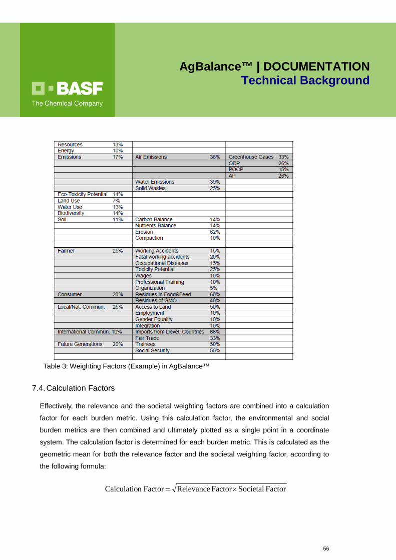
56


Table 3: Weighting Factors (Example) in AgBalance™

7.4. Calculation Factors

Effectively, the relevance and the societal weighting factors are combined into a calculation

factor for each burden metric. Using this calculation factor, the environmental and social

burden metrics are then combined and ultimately plotted as a single point in a coordinate

system. The calculation factor is determined for each burden metric. This is calculated as the

geometric mean for both the relevance factor and the societal weighting factor, according to

the following formula:

Factor Societal Factor Relevance Factor n Calculatio ×=

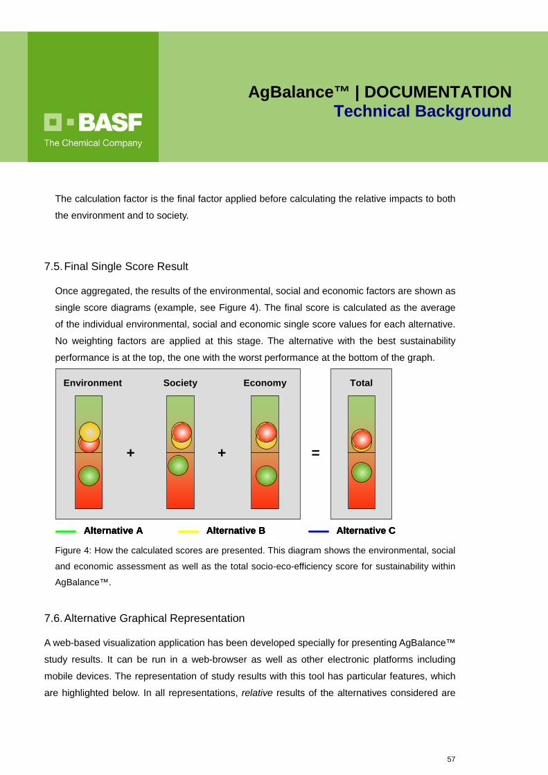
57


The calculation factor is the final factor applied before calculating the relative impacts to both

the environment and to society.

7.5. Final Single Score Result

Once aggregated, the results of the environmental, social and economic factors are shown as

single score diagrams (example, see Figure 4). The final score is calculated as the average

of the individual environmental, social and economic single score values for each alternative.

No weighting factors are applied at this stage. The alternative with the best sustainability

performance is at the top, the one with the worst performance at the bottom of the graph.

Figure 4: How the calculated scores are presented. This diagram shows the environmental, social

and economic assessment as well as the total socio-eco-efficiency score for sustainability within

AgBalance™.

7.6. Alternative Graphical Representation

A web-based visualization application has been developed specially for presenting AgBalance™

study results. It can be run in a web-browser as well as other electronic platforms including

mobile devices. The representation of study results with this tool has particular features, which

are highlighted below. In all representations, relative results of the alternatives considered are

Total

=

Environment Society

+ +

Economy

Alternative CAlternative BAlternative A Alternative CAlternative CAlternative BAlternative BAlternative AAlternative A

58


plotted on normalized scales. The worst alternative in each impact is normalized to one, and the

other alternatives are expressed proportionally, with an improvement indicated by a higher

number.

(1) Individual impact indicator results are shown as points on a normalized scale, represented

as sliders, showing the relative difference between the alternatives considered. For an example

see Figure 5. Points that are higher on the sliders indicate a better result.

Figure 5: AgBalance™ Visualization Tool: Representation of individual indicator results

(2) Normalized results for all impact 16 categories (environmental, social and economic) are

presented in a single graph. Each alternative is represented by petals of a certain color, the

size of the petal being indicative of the relative sustainability performance in the respective

impact category. Larger petals indicate a better result (cf. Figure 6).

59


Figure 6: AgBalance™ Visualization Tool: Representation of impact category results (left) and

single scores of environmental, social and economic dimensions (right).

(3) The three single score results derived for the total environmental, social and economic

impacts, are likewise symbolized, with petals of a certain color representing each alternative

and the size of the petal indicating the relative sustainability performance in the respective

sustainability dimension. Larger petals indicate a better result (cf. Figure 6).

(4) The aggregated total sustainability score of each alternative is represented in a bar chart,

with the worst alternative normalized to one, and the other alternatives expressed

proportionally. Again, the relative improvement is indicated by a larger bar.

60


8. Report Format and Presentation of Results

AgBalance™ methodology, parameters, results and conclusions can be summarized in a

final, written report and/or presentation. At a minimum, these should include a discussion of

the following: Introduction and study goals

Customer benefit, alternatives and system boundaries

Input parameters and assumptions

Method of economic costs evaluation

Method of environmental burden evaluation

Method of social burden evaluation

AgBalance™ analysis results and discussion

Data quality assessment

Sensitivity/uncertainty analysis

Limitations;

References

The study report will show the individual results of the analysis for each of the economic,

environmental and social impact indicators. Impact results should be generated, using

characterized results only i.e. one does not use results that have been normalized or where

the different weighting factors (relevance, societal, E/C, orS/C factors) have been applied.

Weighted and aggregated results for the economic, environment and social burden metrics

are presented as a fingerprint plot, as shown in Figure 3. This diagram shows the

environmental advantages and disadvantages of the considered alternatives, relative to each

other.

At the highest aggregated level, the results of the environmental, social and economic

assessments are presented as Single Score diagrams. This format is also used to illustrate

61


the total socio-eco-efficiency score of the AgBalance™ evaluation (Figure 4). This format

offers a high degree of clarity and has been introduced as a new feature within AgBalance™.

9. Report Limitations

At a minimum, each report or presentation of study results should incorporate the following

disclaimer:

“These AgBalance™ study results and its conclusions are based on specific comparisons of

the production, use, and disposal of alternatives and system boundaries for the described

customer benefit. Transfer of these results and conclusions to other production methods,

regions, applications or products is expressly prohibited. In particular, partial results may not

be communicated so as to alter the meaning, nor may arbitrary generalizations be made

regarding the results and conclusions.”

If this study is expected to be published, a critical review with external partners that have not

been involved in the preparation of the study is required.

10. Limitations of the methodology

An AgBalance™ study takes into account that the database in one country might differ from

others. For this reason, algorithms (e.g., protected area, agri-environmental schemes) as well

as the evaluation and interpretation of results are matched with regional basic conditions.

11. Hot Spot-Analysis

Important aspects that are not covered by the indicators are addressed by a separate,

evaluation e.g., a Hot Spot Analysis. For example, these aspects could be animal welfare,

indigenous rights, malnutrition, etc. Evaluating the sustainability of social impacts is limited

by the definition of a fixed set of indicators. However, a holistic and balanced evaluation of

social sustainability has to consider aspects that might not covered by the pre-defined set of

social LCA indicators. In some cases, these are not easy to quantify, especially those with an

ethical dimension, e.g., malnutrition, indigenous rights, or animal welfare. To address this

62


challenge, the AgBalance™ method assesses potential sustainability risks that are not

covered by the set of quantitative indicators through a Hot Spot-Analysis. , It also provides

recommendations for improvement. This approach enables a great deal of flexibility for the

AgBalance™ methodology without the need to create a consistent method that addresses all

possible issues that might occur in agricultural systems on beforehand.

12. Data Quality Objectives

12.1. Data Quality Statement

The process of developing an AgBalance™ study is often iterative. As data are collected and

more is learnt about the system, new data requirements or limitations may be identified that

require changes to inputs/outputs. The AgBalance™ methodology demands an ongoing

review of the appropriateness, accuracy and preciseness of input data throughout the

duration of the study.

12.2. Sensitivity and Uncertainty Considerations

An AgBalance™ study includes an assessment of the sensitivity and uncertainty in study

inputs and outputs. The scope of this assessment should be based upon the study goals, as

defined in Section 2, and include an evaluation of the quality of the input/output data, relating

to the Relevance and Calculation factors for the study. These factors are specific to each

AgBalance™ study as they are calculated values.

BASF’s AgBalance™ Methodology - NSF International · BASF developed AgBalance™ methodology...

Documents

Transcript of BASF’s AgBalance™ Methodology - NSF International · BASF developed AgBalance™ methodology...