Risø National LaboratoryRoskilde Denmark

The UNEP project CD4CDM

Baseline Methodologies for CDM Projects provides a comprehensive overview of the baseline development for CDM projects. It contains the basics of the baseline; a procedure to propose new baseline methodologies; a status of all new baseline methodologies submitted to the CDM Executive Board and examples of the Methodology Panel’s recommendations on the submitted new baselines; simplified baseline methodologies for small-scale CDM projects; a step-by-step procedure for developing baselines with a demonstration of the application of this procedure in various types of CDM project activities. A separate chapter is dedicated for readers interested to know about the process of establishing baselines for afforestation and reforestation CDM projects.

This guidebook to the CDM is produced to support the UNEP project “Capacity Development for the Clean Development Mechanism” implemented by UNEP Risø Centre on Energy, Climate and Sustainable Development in Denmark. The overall objective of the project is to develop the institutional capability and human capacity for implementation of the CDM in developing countries.

The project is funded by the Netherlands Ministry of Foreign Affairs.

Baseline Methodologies For Clean Development Mechanism Projects

Base

line M

eth

od

olo

gie

s For C

lean

Deve

lop

ment M

ech

anism

Pro

jects

�

Baseline Methodologies For Clean Development Mechanism ProjectsA GUIDEBOOK

UNEP Risø Center, Denmark

Editor

Myung-Kyoon Lee, Keimyung University, Korea

Authors

Ram M. Shrestha

Sudhir Sharma

Govinda R Timilsina

S. Kumar

November 2005

�

Baseline

Methodologies For Clean Development Mechanism Projects

A GUIDEBOOK

UNEP Risø Centreon Energy, Climate and Sustainable DevelopmentRisø National LaboratoryRoskilde, Denmark

Graphic design and production:

Finn Hagen Madsen, Graphic Design, Denmark

ISBN: 87-550-3483-7

The findings, interpretations, and conclusions expressed in this report are en-tirely those of the author(s) and should not be attributed in any manner to the Government of the Netherlands.

�

Table of Contents

Preface .................................................................................................. 7

Chapter I: INTRODUCTION ........................................................................ 8

Chapter II: BASELINES IN CDM ................................................................ 11 2.1 CDM Project Criteria and Eligible CDM Projects ........................11 2.2 Baseline and Its Context in CDM .............................................. 13 2.3 Baselines – Key Elements and Concepts .................................... 15 2.4 Examples of Meth Panel Review Comments on Proposed Methodologies ......................................................... 25 Appendix IIA: GHGs and Sectors covered under the Kyoto Protocol ................................................................... 29 Appendix IIB: List of CDM projects submitted to CDM-EB ............. 30 Appendix IIC: Baseline Literature .................................................... 33

Chapter III: ADDITIONALITY ASSESSMENT .............................................. 38 3.1 Claiming Credits from a Start Date Prior to the Date of Registration ................................................................. 39 3.2 Identification of Alternatives to the Project Activity .................. 40 3.3 Investment Analysis .................................................................. 41 3.4 Barrier Analysis ......................................................................... 44 3.5 Common Practice Analysis ........................................................ 45 3.6 Impact of CDM Registration ..................................................... 46 3.7 Conclusions .............................................................................. 47

Chapter IV: BASELINE FOR SMALL SCALE CDM PROJECTS ...................... 49 4.1 Small Scale CDM Project Criteria and Types .............................. 49 4.2 Identification of Project Additionality ....................................... 53 4.3 Project Categories and Approved Methodologies ..................... 54 4.4 Submitting New Methodology and New Small Scale CDM Project Categories ........................................................... 80

Chapter V: ESTABLISHING BASELINES FOR LARGE SCALE CDM PROJECTS ............................................................................. 84 5.1 Establishing Baselines Using a Pre-approved Baseline Methodology (BM) ..................................................... 81 5.2 Developing a New Baseline Methodology ................................ 86 5.3 Procedures for the Submission and Approval of New Methodologies ............................................................... 114 Appendix VA: Direct and Indirect GHG Impacts ........................... 116

�

Chapter VI: BASELINES FOR AFFORESTATION & REFORESTATION (A&R) PROJECTS ...............................................120 6.1 Sequestration projects .............................................................120 6.2 Determining Eligibility of A&R Projects ....................................122 6.3 Establishing the Baseline for A&R Projects ...............................126 6.4 Agroforestry Project under CDM: An Example .........................137 Appendix VI-A: Description of carbon pools (IPCC) .......................143

Chapter VII:EXAMPLES OF PROJECT SPECIFIC BASELINE METHODOLOGIES .......................................................144 7.1 Grid Connected Power Generation Projects .............................144 7.2 Solid Waste Projects: Consolidated Methodology for Landfill Gas Project Activities (ACM0001) ..........................160 7.3 Industrial Process Improvement Project: Modification of CO2 Removal Process in an Ammonia Plant (AM0018) ...................163 7.4 Fuel Switch Projects: Industrial Fuel Switching from Coal and Petroleum to Natural Gas (AM0008) .........................172 7.5 Energy efficiency projects ........................................................176

Bibliography ............................................................................................177

CDM Baseline Glossary ............................................................................181

APPENDIX: TOOLS & MODELS FOR ESTIMATING BASELINE EMISSIONS ................................................................184

�

List of Tables Table 2-1:Examples of Applicability conditions of approved Baseline Methodologies…………… .........................................................................13Table IIB-1: Biomass Fired Co-generation Project ......................................30Table IIB-2: Landfill Gas Capture Project ....................................................30Table IIB-3: Wind Power Project ...............................................................30Table IIB-4: Hydro Power Project ..............................................................30Table IIB-5: Geothermal Power Project ......................................................30Table IIB-6: Fuel Switching Project ............................................................31Table IIB-7: Energy Efficiency Project .........................................................31Table IIB-8: Waste to Energy Project .........................................................31Table IIB-9: Technology Upgrade in Cement Industry and other industrial processes ................................................................31Table IIB-10: Transport Sector Project .......................................................32Table IIB-11: Capture and destruction of non- CH4 GHGs ..........................32Table IIB-12: Oil and Gas Sector Project ....................................................32Table 3-1: Examples of Additionality Test in the New Baseline Methodology Approved by the CDM-EB ........................................48Table 4-1: Emissions factors for Diesel Generator Systems .........................59Table 4-2: Estimation of Emission Factor for Example 4.3 ..........................65Table 4-3: Estimation of Diesel Consumption for Example 4.6 ...................69Table 4-4: Energy and Emission Baseline Estimation for Example 4.7 .........71Table 4-5: Estimation of Emission Baseline for Example 4.9 ......................73Table IVA-1: Carbon Emission Factors (CEFs) .............................................81Table IVA-2: Selected Net Calorific Values ................................................83Table 5-1: Examples of System Boundaries in Approved Baseline Methodologies ..................................................................98Table 5-2: Examples of Choosing BM Approaches from CDM M&P………………………... ...................................................107TableVA-1: Examples of Accounting the Direct and Indirect Impacts on GHG Emissions ...............................................116Table 6-1: Categorizing land by Land use and Land cover ........................124Table 6-2: Demand displacement analysis for proposed CDM project .....142

�

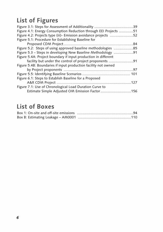
List of FiguresFigure 3.1: Steps for Assessment of Additionality ......................................39Figure 4.1: Energy Consumption Reduction through EEI Projects ..............51Figure 4.2: Projects type (iii)- Emission avoidance projects .......................52Figure 5.1: Procedure for Establishing Baseline for Proposed CDM Project ....................................................................84Figure 5.2: Steps of using approved baseline methodologies ...................85Figure 5.3 – Steps in developing New Baseline Methodology ...................91Figure 5.4A: Project boundary if input production in different facility but under the control of project proponents ........................91 Figure 5.4B: Boundaries if input production facility not owned by Project proponents ....................................................................97Figure 5.5: Identifying Baseline Scenarios ............................................... 101Figure 6.1: Steps to Establish Baseline for a Proposed A&R CDM Project ………….. .........................................................127Figure 7.1: Use of Chronological Load Duration Curve to Estimate Simple Adjusted OM Emission Factor ..............................156

List of BoxesBox 1: On-site and off-site emissions .......................................................94Box B: Estimating Leakage – AM0001 ....................................................110

�

Preface

With the Kyoto Protocol becoming legally binding on 16 February 2005, the Clean Development Mechanism (CDM) is becoming a key instrument for limit-ing greenhouse gas emissions (GHG) and promoting sustainable development. For both developing and developed countries to benefit from the CDM, it is important to establish increased awareness and understanding of its various aspects. Building capacities in the baseline methodology and assessment of GHG emission reductions/sequestration benefits of CDM projects are keys to the suc-cessful development and implementation of the CDM. This guidebook is aimed to address these important issues and thus assist project developers in establish-ing baselines for CDM projects following guidelines based on relevant decisions of Conference of Parties (COP) and CDM Executive Board (CDM-EB) as well as other sources.

The guidebook takes the reader through basic concepts, the processes of devel-oping baseline and baseline methodology, and approval of new baseline meth-odologies. It presents indicative methodologies for small scale CDM projects and examples of approved methodologies for project specific baselines. Further-more, it describes the process of developing baseline for land use and land use change (LULUCF) CDM projects.

This guidebook is produced by the UNEP Risø Center (URC), Denmark, as a part of the project titled Capacity Development for the CDM (CD4CDM), which is being implemented by URC for United Nations Environment Programme (UNEP) through funding from the Ministry of Foreign Affairs, the Netherlands.

The guidebook was written by Ram M. Shrestha, Sudhir Sharma, Govinda R. Timilsina and S. Kumar of the Asian Institute of Technology (AIT), Thailand un-der a URC contract and was edited by Myung-Kyoon Lee.

John Christensen

Head,

UNEP Riso Centre

�

Chapter I

Introduction

The Kyoto Protocol and the Clean Development Mechanism (CDM) came into force on 16th February 2005 with its ratification by Russia. The increasing momentum of this process is reflected in more than 100 projects having been submitted to the CDM Executive Board (CDM-EB) for approval of the baselines and monitoring methodologies, which is the first step in developing and imple-menting CDM projects. A CDM project should result in a net decrease of GHG emissions below any level that would have resulted from other activities imple-mented in the absence of that CDM project. The “baseline” defines the GHG emissions of activities that would have been implemented in the absence of a CDM project. The baseline methodology is the process/algorithm for estab-lishing that baseline. The baseline, along with the baseline methodology, are thus the most critical element of any CDM project towards meeting the impor-tant criteria of CDM, which are that a CDM should result in “real, measurable, and long term benefits related to the mitigation of climate change”.

Two main bodies of literature explain the process for establishing a baseline. One is the guidelines,1 and clarifications of those guidelines for establishing baselines produced by the official agencies responsible for making rules and procedures on CDM – the Conference of Parties (COPs) and CDM Executive Board (CDM-EB). The clarifications are based on issues raised about the guideli-nes as well as on the reviews of the methodologies for CDM projects submitted for approval. The guidelines are perforce generic in nature, as they describe the process for a wide range of CDM projects. The other is the body of research on baselines from researchers and research institutes working on CDM issues. This body of research is focussed on analyzing measures to minimize the possibility of overestimating emissions reductions from CDM projects. Though the guidelines and clarifications are useful in developing baseline methodologies and estab-lishing baselines, due to their very nature, the guidelines are not presented in a form that can be readily used by the newly initiated to the CDM. This guide-book, using the above two bodies of literature on CDM, is aimed at presenting the process for establishing baselines in a user friendly manner and workbook style. It is principally aimed at project developers and developers of baseline and is focussed solely on the process of establishing baselines.

� PleaseseeDecision�7/CP.7inUNFCCCdocumentFCCC/CP/200�/�3/Add.2:Reportofthe

ConferenceofthePartiesonitsSeventhSession(theMarrakechAccord),heldatMarrakechfrom29

Octoberto�0November200�,Addendum,PartTwo:ActiontakenbytheConferenceoftheParties,

VolumeII(http://cdm.unfccc.int/Reference/COPMOP/decisions_�5_�7_CP.7.pdfdated�4thNovember

2004)

�

This guidebook is produced within the framework of the United Nations Env-ironment Programme (UNEP) facilitated “Capacity Development for the Clean Development Mechanism (CD4CDM)” Project.2 This document is published as part of the projects’ effort to develop guidebooks that cover important issues such as project finance, sustainability impacts, legal framework and institutional framework. These materials are aimed to help stakeholders better understand the CDM and are believed to eventually contribute to maximize the effect of the CDM in achieving the ultimate goal of UNFCCC and its Kyoto Protocol. This Guidebook should be read in conjunction with the information provided in the two other guidebooks entitled, “Clean Development Mechanism: Introduction to the CDM” and “CDM Information and Guidebook” developed under the CD4CDM project.3

1.1 The organization of the guidebookChapter 2 of this guidebook begins by highlighting the key CDM project criteria and eligible CDM projects. It further explains the basic concept of a baseline and its context in CDM. It then discusses the key concepts of a baseline and the key elements of a baseline methodology. The chapter also presents examples of comments provided by the CDM-EB on submitted methodologies to highlight the key elements of baseline methodology. A list of projects submitted to the CDM-EB for approval of methodology highlighting the eligible project categories and a review of baseline literature is presented in the Appendix to the chapter.

Chapter 3 of this guidebook presents the tool for assessment of additionality recommended by the CDM-EB for large scale CDM projects. The chapter dis-cusses the application of the tool and highlights the key elements for assessing additionality in proposed CDM projects.

Chapter 4 of this guidebook focuses on small scale CDM (SSC) projects. The chapter first presents the guidelines for SSC and SSC categories recommended by CDM-EB. The chapter then discusses the recommended simplified baseline methodologies for SSC categories along with examples to explain the use of these methodologies. Finally, the process of submission of new project catego-ries and methodologies to the CDM-EB is discussed.

Chapter 5 presents the steps for establishing baselines for large scale CDM proj-ects. Baselines for large scale CDM projects can be established either using exist-ing approved baseline methodologies or by developing a new baseline meth-odology. The chapter first presents use of approved baseline methodologies to

2 ThisprojectisfundedbytheNetherlandsgovernmentandimplementedin�2developingcountries

byUNEPRISØCentrewithcooperationofregionalcentres.

3 Thesedocumentscanbeaccessedathttp://www.cd4cdm.org/publications.html.

�0

establish a baseline for a proposed CDM project. This is followed by a descrip-tion of the steps in developing a new baseline methodology. The discussions on use of an approved methodology and developing a new baseline methodology are illustrated by an example to enhance understanding of the concepts. Finally the chapter presents the procedure for submission and approval of new meth-odologies to CDM-EB.

Chapter 6 focuses on Afforestation and Reforestation (A&R) CDM projects. This chapter discusses the key features of A&R CDM projects that differentiate them from emission reduction projects and the associated rules specific to A&R CDM projects. Further, this chapter presents eligibility conditions for participation, eligible A&R CDM project types, and the process for establishing baselines for A&R projects. This chapter should be read in conjunction with Chapters 2 and 5.

Chapter 7 of the guidebook presents the approved baseline methodologies for grid connected power generation projects, solid waste management projects and industrial process improvement projects. Further, the two approved con-solidated methodologies for landfill gas projects and grid connected renewable energy projects are discussed. The chapter should be read in conjunction with chapter 5 to understand the elements of baseline methodology and use of ap-proved baseline methodologies.

A Glossary of key terms most frequently used in context of CDM and specifically baselines is presented after the bibliography.

The Appendix presents some key models that could be used for estimating the emissions from emissions reduction projects and sequestration by A&R CDM projects.

��

Chapter II

Baselines In CDM

This chapter discusses the context of a baseline in CDM and its key elements. Section 2.1 presents the CDM project criteria and types of eligible projects. This is followed in Section 2.2 by an introduction to the concept of baseline in the context of CDM projects. Section 2.3 presents the key concepts for baselines based on the guidelines for establishing a baseline, as stipulated in the modali-ties and procedures (M&P) of CDM1. Section 2.4 presents examples of Meth-odological Panel’s MethPanel’sReview of selected methodologies submitted to CDM-EB for approval, to highlight the important elements of the baseline methodology.

2.1 CDM Project Criteria and Eligible CDM ProjectsCDM is a project-based mechanism. An important objective of the CDM is to assist developing countries achieve sustainable development2. The responsibil-ity for evaluating the sustainable development contribution of proposed CDM project activities rests with the host (i.e., the developing country that proposes a CDM project). Therefore, in addition to other global CDM criteria, CDM project activities should also satisfy criteria for a sustainable development contribution as defined by the host country’s government.

The three global CDM criteria as outlined in Paragraph 5, Article 12 of the Kyoto Protocol are:

1. The participation of country governments of respective partners in the CDM is voluntary.

2. The projects result in real, measurable, and long term benefits related to mitigation of climate change.

3. The reductions in GHG emissions from the CDM project should be addi-tional to any that would occur in the absence of the CDM (This is referred to as the additionalitycriterion).

� TheCDMM&Pwerefinalizedbytheseventhsessionoftheconferenceofparties(COP7)andthese

aredocumentedintheMarrakechAccord(MA).

2 Interestedreaderscouldalsosee‘CDM:sustainabledevelopmentimpacts’,publishedbyUNEPas

partofCD4CDMproject(www.cd4cdm.org).

��

“Mitigation of climate change” in criterion 2 refers to reducing the increases in greenhouse gases (GHGs) concentration in the atmosphere, which are the cause of long term changes in the climate, and to stabilizing the GHG concentration in the atmosphere. The reduction in concentration of GHGs in the atmosphere can be achieved through reduction of GHG emissions or absorption of GHGs from atmosphere and storing them in a medium. The latter is referred to as sequestra-tion.

Project activities that result in reducing emissions of one or more of the six GHGs3, namely, Carbon dioxide (CO2), Methane (CH4), Nitrous oxide (N2O), Hydrofluorocarbons (HFCs), Perfluorocarbons (PFCs) and Sulphur hexafluoride (SF6), are eligible for CDM. These project activities may reduce GHGs from energy use and production (fuel combustion and fugitive emissions from fuel), industrial processes, use of solvents and other products, the agriculture sec-tor, and waste management. Projects that sequester (store) carbon in biomass, through afforestation and reforestation activities, are also eligible under CDM. The following types of GHG mitigation or sequestration projects and activities can be eligible for CDM:

• Renewable energy technologies

• Energy efficiency improvements - supply side and/or demand side

• Fuel switching (e.g., coal to natural gas or coal to sustainable biomass)

• Combined heat and power (CHP)

• Capture and destruction of methane emissions (e.g. from landfill sites, oil, gas and coal mining)

• Emissions reduction from such industrial processes as manufacture of cement

• Capture and destruction of GHGs other than methane (N2O, HFC, PFCs, and SF6)

• Emission reductions in the transport sector

• Emission reductions in the agricultural sector

• Afforestation and reforestation

• Modernization of existing industrial units/equipment using less GHG-intensive practices/technologies (retrofitting)

3 SeeAppendixAforcompletedescriptionofgasesandsectors.

��

• Expansion of existing plants using less GHG intensive-practices/tech-nologies (Brownfield projects)

• New construction using less GHG-intensive practices/technologies (Greenfield projects)

Criterion 3 states that the proposed CDM project activity should not only result in reduction (sequestration) of GHG, but in reductions beyond those that would have occurred in the absence of the CDM project activity. Even in the absence of CDM, an economy is likely to witness a move towards more efficient energy use and increased renewable energy use. These activities also result in GHG emissions reductions. Therefore, for a project to be an eligible CDM project, the GHG reductions should be greater than or additional to the GHG reductions that are expected to occur in any case. This is also the aspect alluded to by “real” in criterion 2.

“Measurable” reduction implies that a proposed CDM project should result in reductions that can be physically verified.

“Long term benefits” of reduction imply that CDM should result in adoption of practices/technologies that result in a long term trend towards lowering of GHG emissions in the economy. The CDM projects should affect the way energy is produced and/or consumed in the host country economy or should affect a shift towards less carbon intensive energy sources.

While reviewing the above listed categories for eligible CDM projects that use particular processes/technologies, it is important to underscore that these must be processes or technologies that are not expected to be used in similar projects in the normal course in the economy. For example, though wind energy projects result in zero GHG production, they can not be eligible for CDM if wind energy projects are already common in a host country and the proposed CDM project is similar to existing wind projects. In such a case, one would expect that the pro-posed wind energy project would have been implemented even in the absence of CDM. But, if the proposed CDM project is being implemented in, say, a low wind area where in the past no similar projects were implemented, reductions from the proposed project might then be considered additional.

Appendix IIB to this chapter provides tabulation of the CDM projects submitted for approval of methodologies, categorized by project types, to give an idea of types of projects that are eligible under CDM.

2.2 Baseline and Its Context in CDMAs mentioned, CDM projects should result in “measurable” reductions in GHG. Since CDM projects would result in non-negative reductions of GHG emis-sions, the concept of “measurable” reduction is based on a comparison with

��

some defined level of GHG emissions. This comparative level, against which the reductions of GHG emissions due to a CDM project are measured, is termed a "baseline”. The Marrakech Accord defines the baseline for a CDM project activ-ity as “the scenario that reasonably represents the anthropogenic emissions by sources of greenhouse gases that would occur in the absence of the proposed project activity”. Therefore, the baseline is emissions that would have occurred in the absence of CDM project activity. The proposed CDM project will result in reduction of GHG emissions only if the GHG emissions from the proposed CDM project are lower than the baseline.

The scenario defining likely activities/sources of GHG emissions in the absence of a CDM project activity is commonly referred to as the baselinescenario. The term baseline refers to the level or quantity of GHG emissions of an activity or source of emission in the baseline scenario. For example, consider a proposed CDM project for methane gas capture and flaring from a municipal solid waste (MSW) disposal landfill site. Disposal of MSW in landfills results in emission of methane, which is a GHG. In the absence of the CDM project, no action is ex-pected to be taken either to reduce the methane from the MSW landfill site or to capture the methane generated. Therefore, the baseline scenario represents the level of methane generated from MSW disposal in the landfill without the measures for its capture. The baseline for the project is the quantity of methane generated at the MSW disposal in the landfill site.

As defined in Section 2.1, a key criterion for CDM project activities is that emis-sion reduction (sequestration) from a CDM project should be additional to any that would occur in the absence of CDM project activities. The baseline scenario helps establish whether or not the proposed CDM project activity would have been implemented in the absence of CDM and, hence is a test of a project’s additionality. The baseline provides the basis for determining whether GHG emissions (sequestration) from the proposed project are lower (or greater) than the emissions (sequestration) in the absence of the project; that is, whether the CDM project reductions are additional. The baseline scenario and the baseline are thus the bases for testing whether the CDM project activity meets the ad-ditionality criterion.

To recap with the example of a landfill methane capture project, the baseline scenario is release of the methane generated from landfill site into the atmos-phere as there are no incentives or regulations for capturing and flaring the methane emissions. Therefore, the landfill CDM project is an additional activity. The baseline emission, i.e., the methane emission in the baseline scenario, is greater than the methane emissions from the landfill CDM project, which is zero

��

as methane generated is captured and flared4. Therefore, the project emissions reductions are additional.

2.3 Baselines – Key Elements and Concepts The baseline, as discussed above, is the level or quantity of emissions in the baseline scenario as a projection of activities in future that are likely to occur in the absence of the proposed CDM activities. Thus the baseline and the baseline scenario are hypothetical in nature and depend on a number of factors, such as demand for services of the type produced by proposed CDM project, availability of various resources to implement the activity, environmental and other policies relevant to the project activity, etc. Therefore, there is a possibility of multiple baselines for a given proposed CDM project due to the subjectivity involved in interpreting the trends of various factors that influence decisions in the choice of alternatives to the proposed CDM project. To narrow down these subjectivi-ties and provide a common understanding of important aspects to be taken into account while establishing baselines, the modalities and procedures (M&P)5 for CDM, in the Marrakech Accord, give guidelines for establishing the baseline. These guidelines highlight the key concepts for establishing baselines.

2.3.1 Key Concepts for Baselines

This section presents the important concepts related to establishing baselines based on the guidelines in the M&P.

• A baseline should be defined on a project-specificbasis. It should be pre-pared taking into account relevant national and/or sectoral policies and cir-cumstances, such as sectoral reform initiatives, local fuel availability, power sector expansion plans, and the economic situation in the project sector.

• A baseline should cover emissions of all the gases, from all sectors and source categories listed in Annex A to the Kyoto Protocol (Appendix IIA) within the projectboundary.

• The project boundary should encompass all anthropogenic emissions by sources of greenhouse gases: (i) under the control of the project partici-pants; (ii) that are significant; and, (iii) that are reasonably attributable to the CDM project activity.

4 FlaringofmethaneresultsinCO2,whichisaGHG.Sincethecarboninmethaneoriginatesfromorganic

sourcesintheMSWandorganiccarbonissourcedfromtheatmosphere,anyemissionofCO2fromorganicsources

isnotconsideredasemissionbecauseinthefirstplacethecarbonwasabsorbedfromtheatmosphere.

5 http://cdm.unfccc.int/Reference/COPMOP/decisions_�5_�7_CP.7.pdfdated�4thNovember2004.

��

• Reductions in anthropogenic emissions by sources within the project boundary, measured from the baseline emissions, should be adjusted for leakage.

• Leakage is defined as the net change in anthropogenic emissions by sources of greenhouse gases which occurs outside the project boundary, and which are measurable and attributable to the CDM project activity.

• Choices of approach, assumptions, methodology, parameters, data sources, key factors and additionality for developing a baseline should be transpar-ent and should result in a conservative estimate of baseline emissions taking account of uncertainties.

• The baseline may include a scenario where future anthropogenic emissions by sources are projected to rise above current levels, due to the specific circumstances of the host country.

• The baseline should be defined in a way that CERs cannot be earned for decreases in activity levels outside the project boundary or due to force majeure.

• Three baseline approaches have been recommended for choosing a baseline methodology. The project participants should select the most appropri-ate of the three approaches to develop the baseline methodology for their project (These approaches are presented in Section 2.3.2.).

• Project participants shall select a crediting period for a proposed project activity from one of the following alternative approaches: (a) a maximum of seven years which may be renewed at most two times, provided that, for each renewal, a designated operational entity determines and informs the CDM-EB that the original project baseline is still valid or has been updated taking account of new data where applicable; or, (b) a maximum of ten years with no option for renewal.

• All the information used by project participants to determine additionality, to describe the baseline methodology and its application, and to support an environmental impact assessment for the project must be made public and shall not be considered as proprietary or confidential.

Project proponents should establish the baseline for proposed CDM projects us-ing these guidelines. The method/process for establishing the baseline (i.e., the baseline methodology) has to be approved by the CDM-EB prior to its use for establishing a baseline.

For small scale CDM project activities (discussed in Chapter 4), simplified base-line methodologies approved by CDM-EB can be used. These are presented in

��

the document describing simplified modalities and procedures for small-scale CDM project activities.6

Since no CDM-EB approved methodologies were available at the start of CDM, all the proposed CDM projects had to develop new baseline methodologies and have them approved. With time, as the portfolio of approved baseline method-ologies has grown, project participants can develop baselines using an approved baseline methodology which is applicable to their project.

2.3.2 Establishing Baselines – The Key Elements of a Baseline Methodology

The baseline methodology describes the procedure/formulae/algorithm to establish the baseline and assess additionality of the proposed CDM project. The Marrakech Accord guidelines for establishing baselines suggest that in the process of establishing a baseline, the project boundary, the baseline scenario, and leakage from implementation of proposed CDM project activity should be established. Therefore, a baseline methodology is a description of the process of establishing a project boundary, identifying the baseline scenario, steps to prove additionality, steps for estimating emissions, and steps for identifying and esti-mating leakage. The six key elements of a baseline methodology are presented in detail here.

1. Applicability of the baseline methodology

Applicability of baseline methodology defines the conditions under which the baseline methodology can be used to establish a project specific baseline. The conditions provide the context within which the methodology is applied. Fur-ther, a baseline is project specific. However, the methodology used to develop the baseline for a project may be usable for other projects of similar nature. For example, a baseline methodology developed for a landfill gas capture CDM proj-ect in a country could be applicable to similar projects in other countries. Each methodology, as it exists, is developed with a specific proposed CDM project in mind. These projects address very specific measures for reducing GHGs, and operate in given sectoral conditions/characteristics under a given set of poli-cies/regulations. Some or all of these factors affect the baseline scenario and, hence, the baseline. These conditions define the circumstances under which the baseline methodology can be used. Some of the conditions can be parameter-ized and included in the formulae; such conditions do not restrict the applica-tion of the methodology. For example, in the case of the methane capture and flaring project discussed above, the project is established in a country where there are no regulations for capturing and flaring methane. If the baseline emis-sion estimation includes a parameter to represent the fraction of methane to be captured in the baseline as required by law, then the baseline methodology can

� http://cdm.unfccc.int/Projects/pac/ssclistmeth.pdf.dated�4thNovember2004.

��

Table 2-1: Examples of Applicability Conditions of Approved Baseline Meth-odologies.

Methodology Applicability Conditions

AM00017 Incineration of HFC 23 Waste Streams

• The methodology is applicable to any HCFC production facility producing HFC 23 (CHF3) waste streams that is based in a non-Annex I country.

• It is applicable only if there are no regulations restricting the HFC 23 emissions from HCFC production facilities in the country.

AM0002: Greenhouse Gas Emission Reductions through Landfill Gas Capture and Flaring, where the Baseline is established by a Public Concession Contract

This methodology is applicable to landfill gas capture and flaring project activities where:• There exists a contractual agreement that makes the operator

responsible for all aspects of the landfill design, construction, operation, maintenance and monitoring;

• The contract was awarded through a competitive bidding process;• The contract stipulates the amount of landfill gas (expressed in

cubic meters) to be collected and flared annually by the landfill operator;

• The stipulated amount of landfill gas to be flared reflects performance among the top 20% in the previous five years for landfills operating under similar social, economic, environmental and technological circumstances; and,

• No generation of electricity using captured landfill gas occurs or is planned.

AM0003: Simplified Financial Analysis for Landfill Gas Capture Projects

This methodology is applicable to landfill gas capture project activities where:• The captured gas is flared; or, • The captured gas is used to generate electricity, but no emission

reductions are claimed for displacing or avoiding electricity generation by other sources.

• It is applicable only where there are only two plausible alternatives, a business-as-usual scenario (with minor changes and modifications) and the technology used in the proposed project. In other words, the methodology is inapplicable where a plausible alternative is a substantial change in practice or technology different from the proposed technology.

AM0004: Grid-connected Biomass Power Generation that avoidsUncontrolled Burning of Biomass

This methodology is applicable to biomass-fired power generation project activities displacing grid electricity that:• Use biomass that would otherwise be dumped or burned in an

uncontrolled manner;• Have access to an abundant supply of biomass that is unutilized

and is too dispersed to be used for grid electricity generation in the baseline scenario;

• Have a negligible impact on plans for construction of new power plants;

• Are not to be connected to a grid with suppressed demand;• Have a negligible impact on the average grid emissions factor; and,• Where the grid average carbon emission factor (CEF) is lower (and

therefore more conservative as the baseline) than the CEF of the most likely operating margin candidate.

7ThestandardformatusedbyCDM-EBindenotingapprovedmethodology(AM)isAMfollowedbyfourdigitnumber.

��

also be used in countries where there are regulations for capturing and flar-ing methane. On the other hand, if such a parameter is not included, then the methodology is applicable only to countries where there are no regulations for capturing and flaring methane.

Another important constraining factor could be availability of data for use of a baseline methodology. If the data used in the methodology to estimate emissions, baseline, project or leakage are not available in the case of a project, then the methodology is not applicable to that project. The substitution of different sources or types of data for what was stated in the original methodology implies modification of the methodology, which is not permitted.

Description of these applicability conditions helps the evaluation of the baseline methodology. Table 2.1 presents examples of applicability conditions described in baseline methodologies already approved by the CDM Executive Board.

2. The baseline scenario

The baseline scenario describes the activities that would have been implement-ed in absence of the proposed CDM project. The guidance on baseline, dis-cussed in Section 2.3.1, suggests that identification of baseline scenario should capture the likely changes in the project sector/economy due to the national and sectoral policies. For example, selection of baselines for energy efficiency and renewable CDM projects in countries where improvement of energy ef-ficiency and promotion of renewable energy are already part of national energy policy could be different from that in countries where such policies either do not exist or may not be implemented. Moreover, economic and demographic parameters selected in the methodology should be consistent with that pro-vided in national and sectoral policy documents.

The Meth Panel recommended that the following four types of national and/or sectoral policies8 should be considered while developing the baseline method-ologies:

(a) Type E+: existing national and/or sectoral policies or regulations that create policy driven market distortions which give comparative advan-tages to more GHG emission intensive technologies or fuels against less emissions intensive technologies or fuels.

(b) Type E-: national and/or sectoral policies or regulations that create positive comparative advantages to less GHG emission intensive tech-nologies against more emissions intensive technologies (for instance,

8Seedocumenttitled“Clarificationsonthetreatmentofnationaland/orsectoralpoliciesand

regulations(paragraph45(e)oftheCDMModalitiesandProcedures)indeterminingabaselinescenario

(http://cdm.unfccc.int/EB/Meetings/0��/eb��repan3.pdf)

�0

public subsidies to promote the diffusion of renewable energy or to finance energy efficiency programs).

(c) Type L-: sectoral mandatory regulations introduced by local or national public authorities for reduction of local negative environmental exter-nalities and/or energy conservation, which incidentally reduce GHG emissions.

(d) Type L+: sectoral mandatory regulations introduced by local or na-tional public authorities for reduction of local negative environmental externalities, which incidentally prevent the adoption/diffusion of less emitting technology.

Only “Type E+” national and/or sectoral policies or regulations that have been implemented before adoption of the Kyoto Protocol by the COP (Decision 1/CP.3, 11 December 1997) shall be taken into account when developing a baseline scenario. If “Type E+” national and/or sectoral policies were imple-mented since the adoption of the Kyoto Protocol (after 11 December 1997), the baseline scenario should refer to a hypothetical situation without such national and/or sectoral policies or regulations being in place. For example, a host coun-try government has introduced a policy of subsidizing coal in year 1998. While developing a baseline for a wind power project, the project proponent should develop a baseline scenario assuming that no such policy is in place. But, if the same policy were introduced in November 1997, then the baseline scenario should include the implication of the policy on use of the wind resource for generating energy.

“Type E-” national and/or sectoral policies or regulations that have been imple-mented after the adoption by the COP of the CDM M&P (Decision. 17/CP.7, 11 November 2001) do not necessarily have to be taken into account in developing a baseline scenario (i.e., the baseline scenario should refer to a hypothetical situ-ation without the national and/or sectoral policies or regulations being in place). For example, a policy to charge an environment tax on all fossil fuels for elec-tricity generation could make renewable sources competitive vis-à-vis the fossil fuels. Such a policy, therefore, is expected to promote use of renewable sources for electricity generation. If the policy was introduced prior to 11 November 2001, then it should be taken into account while identifying the baseline sce-nario for renewable energy based projects. But, if the policy is introduced after 11 November 2001, as per the above recommendation, its implications for use of renewable energy sources can be ignored.

3. Baseline approaches

Three baseline approaches, described below, have been recommended by the Marrakech Accord in the guidelines for establishing baselines.

��

a) The first approach involves existing actual or historical emissions (hereafter “Approach A”). This is applicable to cases where the analysis of the baseline scenario indicates that the most likely activities imple-mented in absence of the proposed CDM project is the continuation of existing activities. To continue with the Landfill CDM project example, recall that the current practice in the host country is zero collection of methane generated from MSW disposed at the landfills. The analysis of the situation indicates that though there are other options available for curtailing emissions from a landfill (e.g., treatment of organic waste before disposal in a landfill or systems for methane collection at the landfill), the most likely scenario is continuation of present practice. The baseline approach to be used in such a case is Approach A.

b) The second approach (hereafter, “Approach B”) is based on emissions from a technology that represents an economically attractive course of action, taking into account barriers to investment. This approach is applicable to situations, where economic analysis is undertaken to identify most attractive option among various options, which includes the CDM project activity. The emissions from the economically most attractive alternative are the baseline. For the Landfill CDM project example, say the alternatives available are: continuation of the current practice, i.e., zero collection of methane generated from landfill; treat-ment of organic waste before disposal to landfill (methane emissions from landfill are from decay of organic matter); and, a collection system for landfill methane. Suppose the analysis of the situation indicates that treatment of organic waste before disposal at the landfill site is the economically most attractive alternative. Then, the baseline scenario is treatment of organic waste before its disposal to landfill and the base-line approach is Approach B. In this example, the baseline is in terms of emissions from the landfill under the condition that organic waste disposed at the site is pre-treated.

c) The third approach is based on the average emissions of similar project activities undertaken in the previous five years, in similar social, economic, environmental and technological circumstances, and whose performance is among the top 20 percent of their category (hereafter “Approach C”). To continue with the Landfill CDM project, say there are four alternatives, other than the proposed CDM project alternative, available to curtail the methane emission from the landfill. None of the four alternatives can be clearly demonstrated as economically most attractive. The baseline scenario then is based on analysis of alterna-tives implemented during the last five years. The baseline approach in this case will be Approach C. The baseline is the average emission of the options most commonly used in the previous five years and whose performance is among the top 20 percent.

��

The three are akin to options available for implementing a project. Project proponents choose either to continue with an existing commonly used process/technology or to adopt a newer option available in the market that has come to be preferred over a more commonly used option in recent years. If more than one new option is available, the proponents choose the most economical option that meets all the regulatory requirements. But in absence of adequate infor-mation or differences among various new options, any of the options from the basket of new options could be chosen.

Note that these are the approaches to develop a baseline. The formulae or algorithm to estimate emissions under the baseline scenario should be consist-ent with the baseline approach. For example, it is proposed to replace a boiler that provides steam at a facility under a CDM project. If the chosen baseline approach is Approach A, then the baseline emission estimation formulae will consist of formulae for estimating emission from use of the existing boiler. If Approach B is chosen, then the formulae for estimating baseline emission will be for the boiler type that is most economical. For Approach C, the formulae for estimating baseline emissions will be the average emissions of the types of boiler used by recent projects of similar kind in the last five years.

The baseline approach for Afforestation and Reforestation projects are discussed in Chapter 6.

4. Baselines

The baseline is the emission in absence of the proposed CDM project. Baseline describes the formulae for estimating the emissions in the identified baseline scenario for the proposed CDM project. It also includes the description of source of data for parameters/variables.

5. Project additionality

Additionality is the key element of the baseline methodology. There are two components of additionality that should be satisfied by a proposed CDM proj-ect.

(i) The project emissions (sequestration) are less (greater) than the baseline emissions (sequestration).

(ii) The proposed project should not be a baseline option.

A methodology should include steps to analyze the additionality of the proj-ect. The CDM-EB has prepared a consolidated tool for assessing additionality (discussed in Chapter 3). The tool suggests the following steps for assessment of additionality:9

��

(i) Identification of alternatives to the project activity.

(ii) Investment analysis to determine that the proposed project activity is not the most economically or financially attractive option.

(iii) Barriers analysis.

(iv) Common practice analysis.

(v) Impact of registration of project as a CDM project on the investment and other barriers faced by the project.

The CDM-EB suggested tool for assessment of additionality is not mandatory. Project proponents can develop their own process for establishing the addi-tionality of a proposed CDM project.

6. Leakage

The term leakage refers to emissions occurring outside the “project bound-ary” that are directly attributable to the proposed CDM project activity and are measurable. For example, emissions due to transportation of biomass fuel to the proposed CDM biomass power project site are a project leakage. The project boundary for the project is the physical site of the power plant. There-fore, the transport related emissions are outside the project boundary. Trans-portation of biomass fuel is a direct consequence of the biomass power plant and, therefore, is attributable to the project. It is necessary to identify possible leakage in emissions in the baseline methodology. If the leakage is measurable and significant, methods (i.e., equations or formulas) to estimate the leakage should be presented in the baseline methodology.

2.3.3 Key Criteria for Establishing Baselines

Apart from the above mentioned key components of the baseline methodol-ogy, the guidance also gives key criteria for establishing baseline. These criteria are important to ensure that baseline is established so that the objectives of CDM are fulfilled. The two key criteria are transparency and conservative esti-mation of baseline.

1. Transparency

The baseline methodology should be transparent in each step of its develop-ment. The transparency criterion requires that the methodology should also be replicable by third party based completely on the information provided in the methodology documentation. All data sources, references and assumptions

9“ToolfordemonstrationandassessmentofAdditionality”.http://cdm.unfccc.int/methodologies/

PAmethodologies/Additionality_tool.pdf(ason25thApril2005).

��

used in developing the baseline should be identified and properly documented.

2. Conservatism

Conservatism implies that the assumptions and choice of parameters should be such that baseline emissions estimated should be on the lower rather than higher side. The conservative aspect of baseline methodology is linked to choice of assumptions and key parameters. It is also associated with uncertainties in baseline scenario, i.e., assessment of possible future measures, whose outcomes might be unknown at present.

2.3.4 Key Parameters, Assumptions and Uncertainty

The conservativeness and transparency of methodology is linked to the choice of values for key parameters and the assumptions made. A number of assump-tions with respect to various elements of baseline methodology and parameters (e.g., carbon content of fuel used) used in estimating emissions are likely to be made while developing the baseline methodology. The estimates of baseline emissions will be significantly affected by these assumptions and parameters. Therefore, key parameters and assumptions particularly in terms of data sources should be clearly stated and chosen so that they result in a conservative esti-mate. Their identification also helps baseline developers to check the robustness of the methodology and its appropriateness for the specific project for which it is developed. For example, the choice of emission coefficient for fossil fuel used could be project specific or generic for the country/region adopted from Inter-governmental Panel on Climate Change (IPCC)10 publications. If reliable project specific data are available, that should be used to estimate emission coefficient. But if the country specific data are of low reliability and IPCC default values are the only available sources of information, then the choice should be made keeping in mind the conservative principle. If the methodology uses a particular method for estimating the emissions, for example weighted average of emissions from all the emissions sources in baseline scenario, the underlying assumptions behind the choice of weights used for averaging should be stated. The choice of assumption should be guided by conservative principle within the realms of a realistic assumption.

Another important factor is how uncertainty in various key parameter values is addressed by the methodology. A baseline scenario includes certain assump-tions about the activities in the project/sector in the future. These assumptions introduce uncertainties in the estimated baseline. The methodology needs to highlight each and every possible uncertainty embedded in the baseline sce-nario. The identification of uncertainties is useful to minimize the impact of uncertainties on baseline. Hence, a baseline methodology should clearly identify uncertainties and include discussions of elements that minimize uncertainties.

�0 www.ipcc.ch

��

2.4 Examples of Meth Panel Review Comments on Proposed Methodologies The review comments of Meth Panel or CDM-EB on the submitted method-ologies can be a very useful guide to project participants in developing base-line methodologies. Some examples of the comments on selected proposed methodologies, which have been approved by the CDM-EB, are discussed here. For each of the methodology included here first the main GHG impact of the project is described. Following this a brief description of the methodol-ogy issue is stated, on which the Meth panel has commented, and followed by the comments of Meth Panel (in italics). As the Meth Panel comments use the context of sections and sub-sections in CDM project design document (CDM-PDD), further explanations are added within the comments to give the context.

Note that the methodologies referred to in this section were submitted in a format different from the present format for submission of new methodologies, which became applicable after July 2004. The description of the new method-ology for baseline in the old format was included as Annex 3 to the CDM-PDD and that for monitoring methodology was Annex 4. Therefore, reference to Annex 3 and Annex 4 in the following sections should be understood as Annex to the CDM-PDD and not this guidebook.

2.4.1 Vale do Rosario Bagasse Cogeneration Project in Brazil

Vale De Rosario Bagasse Cogeneration Project proposes to install high effi-ciency boilers to use its surplus bagasse from sugar crushing units and generate electricity for supply to the grid. As the project uses sustainable biomass, it will result in emission reduction by displacing power generation that includes generation sources using fossil fuel.

The baseline approaches used are Approaches A and B. The choice of approach is stated without any reasoning.

JustificationmustbeprovidedontheselectionoftheapproachunderPara48oftheCDMM&Pthatthemethodologyconsidersasthemostappropriateforthecaseofgridconnectedbagassecogenerationprojectactivities.

The baseline methodology does not provide any specific step for assessing ad-ditionality of the project in Annex 3 to the PDD of the proposed project. The additionality is stated through general statements on the power sector situa-tion in the main body of CDM-PDD.

Themethodologypresenteddoesnotaddressthedeterminationofwhethertheprojectactivityisnotpartofthebaselinescenario(ad-ditionality)explicitly,……..Methodologyshouldclearlyaddressthe

��

procedureforsubstantiatingtheadditionalityquestion,viaprocedureofquestions,barrieranalysis,etc.

2.4.2 Nova Gerar Landfill Gas to Energy Project in Brazil

The Nova Gerar Landfill Project proposes to build a gas collection mechanism at an existing landfill site in Brazil, use the collected gas to generate electricity, and supply the electricity so produced to the grid. The methane in the gas is burned in the generation system and results in release of CO2. The CO2 emis-sion related to flaring of methane are not considered, as the carbon in meth-ane is from the organic content of waste disposed at site. The project results in avoiding methane emissions as well as emissions from the power generation sources displaced in the grid due to the power generation from project.

The baseline approach used in the PDD is Approach B. Simplified financial analysis is used to identify the baseline scenario. The analysis based on current practices and current and foreseeable regulations indicate that the only alter-native to CDM project is no collection and utilization of gas (BAU alternative).

The new methodology does not clearly state the process of establishing a project boundary. As a result the following comment was made:

Proceduresfordefiningthesystemandprojectboundaries:Theseareprovidedonlyintheprojectspecificapplication(SectionBofCDM-PDD), and are absent from methodology (Section 4 in Annex 3 toCDM-PDD).

In the PDD the additionality is demonstrated through financial analysis and comparison of internal rate of return (IRR) with threshold value of IRR. If IRR of the project is less than the threshold value of IRR, the project is not a base-line scenario project. But this is only stated in the main body of CDM-PDD and not clearly defined in Annex 3 to CDM-PDD. Though the baseline methodo-logy states conservative estimate of IRR will be made; it does not clearly state how it will be ensured. The baseline methodology states the threshold value of IRR without explaining the process of selecting it; hence the following:

Pleaseprovideguidance(evenifbrief)astohowthis(conservativeIRR)willbeappliedandassured,e.g.whetherlowervalueswillbeusedforeachassumption?Howwillconservatismoftheseassump-tionsbereviewed?ForinstancecanhighandlowvaluesforthefinancialparametersgiveninAnnex5(totheCDM-PDD)beshownalongsidethevaluesselected?

��

2.4.3 Graneros Plant Fuel Switching Project in Chile

The Graneros Project plans to replace coal and other fuel at its plant by natural gas. The project PDD uses both Approaches A and B. But the baseline scenario is the continuation of use of coal in the plant, which is based on Approach A. This led to the following comment by the Meth Panel:

“Theproposedmethodologyshoulduseonlyoneapproach(48(a)-Approach A),referringtothecalculationofemissionreductions.ThissingleapproachshouldbeclearlyindicatedandappliedintheCDM-PDD.”

In the PDD baseline emissions is estimated as the carbon content of coal used for energy at the plant, fugitive emission from coal mining and emission related to transport of coal to the plant site. The formulae for estimation are stated in detail in the PDD but not mentioned in the new baseline methodology section. This is pointed out in the following comment by the Meth Panel:

Manyformulae/algorithmsandspreadsheetshavealreadybeenincludedinthemethodology(described in the main body of CDM-PDD)–ensurethatallareincludedinAnnexes3and4(of CDM-PDD),not[only]intheCDM-PDD.

The methodology in the PDD described the emission factor for fuels and the fuel consumption as the key parameters. But, it neither explains the process for arriv-ing at the key parameters nor states some other key parameters, such as growth in fuel consumption in baseline, relative fuel prices, etc. This led to a comment by the Meth Panel as follows

Themethodofestablishingkeyparametershouldbeoutlinedexplicitlyinthebaselinemethodology(Annex3 of CDM-PDD).Inapplyingthemethodologytotheprojectactivity,afactorof2.5%isderivedasbeing“likelytobealower-boundoftheexpectedemissionreductions(TheannualaveragegrowthrateofcoalconsumptionattheGranerosplantwas4.4%peryear,forthe�998-2002period.)”.However,algorithmtoderivethelowerboundisnotstated,noristhefactorderivedinthespreadsheets(submitted with the CDM-PDD).

2.4.4 Wigton Wind Farm in Jamaica and the Caribbean Region

The purpose of the project is to implement the first commercial scale grid con-nected wind power plant in Jamaica and the Caribbean region. According to the PDD, the project will lead to reduced greenhouse gas emissions as it will displace largely fossil fuel based electricity in the generating system. The CDM-EB suggested the methodology to be resubmitted after addressing the issues raised by the review comments of Meth Panel.

��

The methodology in Annex 3 of the project’s PDD describes the data used for project. The methodology description should be restricted to explaining the steps and formulae, whereas, the CDM-PDD is the place to describe how the formulae is used and what data/parameters are used. If some of the parameters for the methodology are fixed, then those can be stated in Annex 3.

Removeprojectsreferences,project-specific(i.e.Jamaican)data,datasourcesandotherconsiderationsfromAnnexes3(of CDM-PDD),sincethemethodologyshouldbegeneric.

Thestep-by-stepexplanationofthemethodologyprocedurefoundinSectionB(of CDM-PDD)shouldbeprovidedinAnnex3(of CDM-PDD),withexplanationofhowsituationsofinadequateorunreliabledatashouldbehandled,sothatapplicationsofthismethodologyinothercircumstancesisdoneinaconsistentmanner.

The methodology provides the formula for estimating baseline emission factor, which is :

Total emissions in year x = ∑t (Op x Pt) x CEFt

where: t = Fuel used per technology used; Op = Output of the project; Pt = Pro-portion of technology and fuel use as compared to the total mix; CEFt = Carbon emissions factor for the technology used in absence of the CDM project. This gives an impression that all power generation plants are included, whereas, the methodology steps state that only the most recently added plants are consid-ered. This led the Meth Panel to make the following comment:

ImprovepresentationandprecisionofthealgorithmsprovidedinSec-tion5ofAnnex3.ItshouldbeclearthattheoverallCEFisgenera-tion-weightedaverageoftheemissionratesofrecentadditions.

��

Appendix II A: GHGs and Sectors covered under the Kyoto Protocol (Annex A of Kyoto Protocol)

Greenhouse gases1. Carbon dioxide (CO2)2. Methane (CH4)3. Nitrous oxide (N2O)4. Hydrofluorocarbons (HFCs)5. Perfluorocarbons (PFCs)6. Sulphur hexafluoride (SF6)

Sectors/source categories• Energy

• Fuel combustiono Energy industrieso Manufacturing industries and constructiono Transporto Other sectorso Other

• Fugitive emissions from fuelso Solid fuelso Oil and natural gaso Other

• Industrial processes• Mineral products• Chemical industry• Metal production• Other production• Production of halocarbons and sulphur hexafluoride• Consumption of halocarbons and sulphur hexafluoride• Other

• Solvent and other product use• Agriculture

• Enteric fermentation• Manure management• Rice cultivation• Agricultural soils• Prescribed burning of savannas• Field burning of agricultural residues• Other

• Waste• Solid waste disposal on land• Wastewater handling• Waste incineration• Other

�0

Appendix II B: List of new baseline and monitoring methodologies

submitted to CDM-EBTable IIB-1: Biomass Fired Co-generation Project

NM0001: 35 MW Vale do Rosario Bagasse Cogeneration (VRBC) Project, Brazil

NM0018: 3 MW Metrogas Package Cogeneration Project Chile

NM0019: 3 MW Grid-connected Biomass Power Generation that avoids Uncontrolled Burning of

Biomass, Thailand

NM0030: 20 MW Haidergarh Bagasse Based Co-generation Power Project, Uttar Pradesh, India

NM0050: Ratchasima small power producer expansion project, Thailand

NM0060: Dan Chang Bio-energy Cogeneration Project, Thailand

Table IIB-2: Landfill Gas Capture ProjectNM0004: Salvador Da Bahia Landfill Gas Project, Brazil

NM0005: Nova Gerar landfill gas to energy project, Brazil

NM0010: Durban landfill-gas-to-electricity project, South Africa

NM0021: CERUPT Methodology for Landfill Gas Recovery, Brazil

NM0022: Methane capture and combustion from swine manure treatment for Peralillo, Chile

NM0034: Granja Becker Greenhouse Gas (GHG) Mitigation Project, Minas Gerais, Brazil

NM0038: Methane Gas Capture and Electricity Production, Chisinau Wastewater Treatment Plant,

Moldova

Table IIB-3: Wind Power ProjectNM0012: 28 MW Wigton wind farm project, Jamaica and the Caribbean Islands

NM0024: 19.3 MW Jepirachi Windpower Project, Columbia

NM0036: 120 MW Zafarana Wind Power Plant Project, Egypt

Table IIB-4: Hydro Power ProjectNM0020: 32 MW La Vuelta and La Herradura hydroelectric Project, Columbia

NM0023: 30 MW- El Gallo hydro power project, Mexico

NM0043: 98 MW Bayano Hydroelectric Project, Panama

NM0051: Small Hydropower Plant Feeding into a Hydro Dominated Grid, Brazil

NM0054: Simimbe Hydropower Project, Ecuador

Table IIB-5: Geothermal Power ProjectNM0053: Lihir Geothermal project, Papua New Guinea

NM0055: Darajat Unit III Geothermal Project, Indonesia

��

Table IIB-6: Fuel Switching ProjectNM0016: Graneros plant coal to gas fuel switching project, Chile

NM0026: Rang Dong Oil Field Associated Gas Recovery and Utilization Project, Vietnam

NM0029: V&M do Brasil Avoided Fuel Switch Project, Minas Gerais, Brazil

NM0048: Indocement’s Sustainable Cement Production Project (fuel switching component),

Indonesia

NM0062: APCL Electricity Generation Project with Cleaner Fuels (Natural Gas), India.

Table IIB-7: Energy Efficiency ProjectNM0017: Steam system efficiency improvements in refineries in Fushun, China

NM0037: Energy efficiency through installation of modified CO2 removal system in Ammonia Plant, UP, India

NM0042: Water pumps Energy Efficiency Improvements in Municipal Water Utilities in Karnataka, India

NM0044: Power factor correction in water pumps in Municipal Water Utilities in Karnataka, India

NM0046: Andijan District Heating Project, Uzbekistan

NM0058: Energy Efficiency Improvements- Hou Ma District Heating System, Shanxi Province, China

NM0059: Optimization and co-generation of energy from steel making process, Brazil

Table IIB-8: Waste to Energy ProjectNM0031: OSIL - 10 MW Waste Heat Recovery Based Captive Power Project, India

NM0032: 5.6 MW Municipal Solid Waste Treatment cum Energy Generation, Lucknow, India

NM0039:Bumibiopower Methane Extraction and Electricity Generation, Malaysia

NM0041: Korat Waste To Energy Project, Thailand

NM0049: BOF Gas Waste Heat Recovery, Karnataka, India

NM0056: Vinasse Anaerobic Treatment Project - Compañía Licorera de Nicaragua, S. A. Nicaragua

NM0063: Organic Green Waste Composting, Bangladesh

Table IIB-9: Technology Upgrade in Cement Industry and other industrial processes

NM0033: Holcim Costa Rica’s Cartago Cement Plant, Technology Upgrade Project, Costa Rica

NM0045: Birla Corporation Limited: CDM project for “Optimal Utilization of Clinker and

Conversion Factor Improvement, India

NM0047: Indocement’s Sustainable Cement Production Project (Blended cement component), Indonesia.

NM0061: N2O Emission Reduction Project in Onsan, South Korea

Table IIB-10: Transport Sector ProjectNM0052: Urban Mass Transportation System, Bogota, Columbia

Table IIB-11: Capture and destruction of non- CH4 GHGsNM0007: Incineration of HFC 23 Waste Streams from HCFC production Facilities, Republic of Korea

Table IIB-12: Oil and Gas Sector ProjectNM0066: Nanshan Coalmine Methane Utilization Project, China

��

Appendix II C: Baseline Literature

Studies related to establishment of baselines for CDM project activities can be classified into three categories. The first type of study is the one financially supported by international organizations such as OECD/IEA, UNIDO, UNDP and UNEP. These are produced as a result of broader capacity building projects for the CDM in general or for the baseline development in particular. The ‘User Manual for Baseline Assessment’ produced by the UNIDO as a result of its study entitled ‘Guidelines to Support Decision-making on Baseline-setting and Ad-ditionality Assessment for Industrial Projects’ is a good example in this category. Moreover, under the CERUPT program of the Dutch government, a guidebook entitled ‘CERUPT Guideline: Vol.1 Introduction; Vol.2a Baseline Studies, Mo-nitoring and Reporting; Vol. 2b Baseline Studies for Specific Project Categories; Vol. 2c Baseline Studies for Small-Scale project Categories’ has been published by Ministry of Housing, Spatial Planning and Environment of the Netherlands7. Besides these, a few baseline studies have been conducted by researchers and academician and published in academic journals (e.g., Parkinson et al, 20018; Roy et al, 2002; Shrestha and Shrestha, 20049;Shrestha and Abeygunawardana, 200410). The second type of baseline study is the one produced in the process of proposing new baseline and monitoring methodologies to the CDM-EB. Mainly private consultants or CDM project participants themselves are involved in these baseline studies. Several new baseline and monitoring methodologies have been submitted to the CDM-EB to date. These baselines studies are frequently refer-

7TheGovernmentoftheNetherlandshasdecidedtomeet50%oftheemissionreductionsthrough

JI(25%)andCDM(25%).Oneofthestrategiestoachievethisgoalistobuyemissioncreditsthrough

atenderprocedure.TheDutchimplementingagency,Senter,hasalreadystartedtheproceduresince

November200�.Senterbuyscarboncreditsthroughtwodifferentprocurementprograms,theERUPT

andCERUPT.ERUPTisforcarboncreditsgeneratedfromCentralandEasternEuropeunderJI;whereas

CERUPTisforcreditsgeneratedfromdevelopingcountriesundertheCDM.Carboncreditsgeneratedfrom

renewableenergy,energyefficiency,fuelswitchingandwastemanagementwouldbeprocuredunderthe

programs.TheCERUPTprogramallowsbanking(i.e.,creditsachievedbetweennowand2008wouldbe

procured),whereasERUPTdoesnotallowbanking.Theminimumscopeofsupplyduringthetermofthe

contractis500,000tCO2einthecaseofERUPTand�00,000tCO2einthecaseofCERUPT(Martenset

al.200�b).

8Parkinson,S.,K.Begg,P.BaileyandT.Jackson(200�),‘AccountingforFlexibilityagainstuncertain

Baselines:LessonsfromCaseStudiesintheEasternEuropeanEnergySector’,ClimatePolicy,Vol�.No.�,

pp.55–73.

9Shrestha,R.M.andShrestha,R.,2004.Economicsofcleandevelopmentmechanismspowerprojects

underalternativeapproachesforsettingbaselineemissions,EnergyPolicy,Vol32,No�2,pp.�3�3

–�374.

�0Shrestha,R.M.andAbeygunawardana,A.,2004.CO2emissionreductionduetorenewable

generationprojectsundercompetitiveelectricitymarket,paperpresentedat24thAnnualNorthAmerican

ConferenceofUSAEE/IAEE,8-�0July2004,WashingtonDC,USA.

��

red to in various sections of this report. Besides, some international institutions and private consulting companies have also developed and published guide-books for CDM project activities. Baseline development is treated as one of the key components in these guidebooks. These studies can be classified as the third type of baseline studies.

A number of baseline studies have been carried out in recent years by internati-onal organizations and academic/research institutions. Some of these are briefly introduced below:

UNIDO (2003): The United Nations Industrial Development Organization (UN-IDO) has initiated a study ”Guidelines to Support Decision-making on Baseline-setting and Additionality Assessment for Industrial Projects” to provide a foun-dation for the development of a methodological tool that supports the analysis of data and information for setting emissions baselines for industrial projects. As a result of the study, a user manual for baseline assessment together with a soft-ware tool has been produced11. The user manual and the software are expected to help improve the quality of baseline assessment methods and reduce the high transaction costs embodied in the uncertainty, time and risk associated with the potential failure of a project to generate certifiable reductions.

Roy et al (2002)12: This study develops sectoral baselines for the power sector in the Eastern Regional Electricity Grid in India. Four different approaches based on carbon intensity (kgC/kWh) are applied to determine the baseline. These approaches are: (i) average sectoral trend during the last 4-6 years or decade; (ii) generation fuel type (i.e., coal based, oil based, hydro, nuclear); (iii) ownership types and (iv) project specific performance.

Kartha et al. (2002)13: This study identifies workable methodologies to stan-dardize baselines for grid connected electricity CDM projects. It discusses the different types of baseline approaches (i.e., operating margin, build margin and combined margin) for CDM projects that supply electricity to the national or regional grids. The discussions are more focussed on the “combined margin” approach, which is a combination of “build margin” (i.e. replacing a facility that would have otherwise been built) and “operating margin” (i.e. affecting the operation of current and/or future power plants).

�� UnitedNationsIndustrialDevelopmentOrganization(UNIDO)(2003),GuidelineDocumentFinal

EditionV�.0,Vienna.

�2 Roy,J.,S.Das,J.SathayeandL.Price(2002),EstimatingBaselinesforCDM:CaseofEastern

RegionalGridinIndia,EnvironmentalEconomicsandPolicyStudies,Vo.5,Pp.�2�-�34.

�3 Kartha,S.,M.LazarusandM.Bosi(2002),PracticalBaselineRecommendationsforGreenhouseGas

MitigationProjectsintheElectricPowerSector,InformationPaper,ORDandIEA,Paris.

��

NETL (2001)14: The National Energy Technology Laboratory of the U.S. Depart-ment of Energy conducted two studies on the establishment of baselines for market-based mechanism. The first study—“Developing Emission Baselines for Market-Based Mechanisms: A Case Study Approach”— examines three major emission baseline approaches i.e., the project-specific approach, the benchmark approach, and the modified technology matrix approach. The second study- fur-ther examines the modified technology matrix and develops such matrices for India and Ukraine.

OECD/IEA (2000)15: This work presents studies on construction and standardiza-tion of baselines undertaken by the Annex I Expert Group. The case studies pre-sented are for cement, electricity generation and iron and steel industries. Case of China, India and Czech Republic include the cement industry baseline study. While case studies of Brazil, India and Morocco include the electricity industry baselines, case studies of Brazil, India and Poland are included in iron and steel industry baselines.

Lazarus et al. (1999)16: This study explores benchmarking approaches to con-struct acceptable baseline for CDM project activities. It evaluates a series of potential benchmark methodologies using readily available data in five countries – Argentina, China, South Africa, Thailand and the United States17. The overall goal of the study was to identify (i) the most promising methods for setting benchmark baselines and (ii) the sectors and project categories most conducive to the benchmark approach. The study discusses five benchmark approaches: (i) average, aggregate power sector benchmarks, (ii) better-than-average bench-marks (e.g., better than 50th percentile); (iii) recent capacity additions that provide an estimate of the generation displaced by a CDM project that is more accurate than is provided by all existing capacity; (iv) disaggregated approaches (i.e., benchmarks specific for fossil-fuel plants, for base-load versus peak-load facilities) and (v) hybrid approaches that couple some project-specific and benchmark baselines.

�4 NationalEnergyTechnologyLaboratory(NETL)(200�),DevelopingEmissionBaselinesforMarket-

BasedMechanisms:ACaseStudyApproach,andDevelopingtheTechnologyMatrixforIndiaandUkraine,

NETL,

�5 OrganizationofEconomicCooperationandDevelopment(OECD)/InternationalEnergyAgency(IEA)

(2000),EmissionBaselines:EstimatingtheUnknown,OECD/IEA,Paris.

�� Lazarus,M.,S.Kartha,M.Ruth,C.DunmireandS.Bernow(�999),EvaluationofBenchmarkingas

anApproachforEstablishingCleanDevelopmentMechanismBaselines,TellusInstitute,Boston.

�7 EventhoughtheUnitedStatescannotbeaCDMprojecthost,itwasselectedasoneofthesample

countriessimplybecausetheavailabilityandqualityofelectricsectordatasurpassesthatofanyofthe

non-AnnexBsamplecountries,makingitagooddemonstrationofthelevelofanalysisthatispossibleif

gooddataisavailable.

��

Martens et al. (2001a)18: The main objective of this study was to develop simple methods for baseline setting, monitoring and verification (M&V), and other CDM-related processes. The study considered off-grid generators, grid extension, and selected traditional energy technologies for households (e.g., kerosene and car batteries).

Martens et al. (2001b)19: This study develops standardized baselines for small-scale projects in order to facilitate small-scale CDM project activities under the various programs of the Dutch Ministry of Housing, Spatial Planning and Envi-ronment, particularly ERUPT and CERUPT. It presents standardized baselines for five types of CDM projects. Besides these studies, various international and national organizations have started to publish CDM guidebooks or CDM project manuals. Some of these guidebooks/manuals are the following:

1. CDM Information and Guidebook, UNEP RISØ Center, 2003.

2. An Implementation Guide to the Clean Development Mechanism, Unit-ed Nations Conference on Trade and Development (UNCTAD), 2003.

3. A User’s Guide to the CDM (Clean Development Mechanism), 2nd Edi-tion’, Pembina Institute for Appropriate Development, Canada, 2003.

4. The e7 Guide to Implementing Projects under the Clean Development Mechanism, e7 Climate Change Working Group, 2003.

5. CDM Project Manual, Danish Energy Authority, 2003.

6. The Clean Development Mechanism (CDM), A Brazilian Implementa-tion Guide, FGV Editora, December 2002.

7. Laying the Foundations for Clean Development: Preparing the Land Use Sector, A Quick Guide to the Clean Development Mechanism, IIED, ECOSECURITIES and ECCM, 2002.

8. Clean Development Mechanism: A Guide for Potential Participants in South Africa, AEA Technology plc and Energy Research Institute (ERI)

�8 Martens,J.W.,S.L.Kaufman,J.GreenandF.D.J.Nieuwenhout(200�a),StreamliningCDM

ProceduresforSolarHomeSystems:AReviewofIssuesandOptions,ECN,TheNetherlands.

�9 Martens,J.W.,S.N.M.VanRooijen,V.BoveeandH.J.Wijnants(200�b),Standardized

BaselinesforSmall-ScaleCDMActivities,AProposalfortheCDMProgramoftheNetherlands,Discussion

Paper,ECN,TheNetherlands.

��

University of Cape Town, 2002.

9. Clean Development Mechanism (CDM), Manual, United Nations Development Program, 2002.

10. CERUPT Guideline: Vol. 2a Baseline Studies, Monitoring and Reporting; Vol.2b Baseline Studies for Specific Project Categories; Vol.

2c Baseline Studies for Small-Scale Project Categories, Ministry of Housing, Spatial Planning and Environment of the Netherlands, 2001.

11. Project Developer’s Guide for the CDM, United Nations Development Program, 2000.

��

Chapter III

Additionality Assessment

Additionality is one of the complex issues of CDM modalities and procedures. Additionality has been interpreted in many different ways. The CDM-EB, in its 16th meeting, made clarifications on elements of additionality and approved a consolidated tool to assess additionality.1 Based on clarifications of the CDM-EB there are two elements of additionality that should be satisfied by a CDM project.

(i) The project emissions (sequestrations) are less (greater) than the baseline emissions (sequestrations).

(ii) The proposed project should not be a baseline option, i.e., compared to the identified alternative baseline scenarios, the proposed CDM project is the least likely.

The consolidated tool essentially provides guidance on assessing the additional-ity component mentioned in (ii) above. The CDM-EB has clearly stated that use of the tool is not mandatory. Project proponents can develop their own meth-odology for assessing additionality of the proposed project, but it is essential that such a methodology provide steps to prove the above two aspects of addi-tionality. In this chapter we present the various steps involved in the assessment of additionality based on CDM-EB recommended tool. The various steps and the sections where these are discussed are shown in Figure 3.1. The endeavor is to highlight the important elements of additionality assessment using the tool. The underlying philosophy of this tool is that a proposed CDM project activity is a baseline scenario unless otherwise proven.

� ToolfordemonstrationandassessmentofAdditionality.http://cdm.unfccc.int/methodologies/

PAmethodologies/Additionality_tool.pdf(ason25thApril2005).

��

Figure 3.1: Steps for assessment of additionality

3.1 Claiming Credits from a Start Date Prior to the Date of Registration –Step 0This step (hereafter, Step 0) is undertaken only if the project proponents want to claim credits from a start date (say, 1st January 2004, when the project became operational) prior to the registration date of the project (say, 1st July 2005). This facility is available only for those projects that register before 31st December 2005. Such projects should prove that

• The starting date of the project activity falls between 1 January 2000 and the date of the registration of a first CDM project activity (first CDM project was registered on 18 November 2004).

��

• The incentive provided by the CDM was seriously considered in the deci-sion to proceed with the project activity. This evidence should be based on (preferably official) documentation clearly showing that the CDM incentive played a role at or before the time of decision making.

3.2 Identification of Alternatives to the Project Activity Consistent with Current Laws and Regulations–Step 1This step requires defining and identifying realistic and credible alternatives to the project activities that can be the baseline scenario. The following steps de-fine the process through which baseline scenarios can be identified.

Sub-step 1a. Define alternatives to the project activity:

A list of realistic and credible alternative(s) available to the project participants that can provide outputs or services comparable with the proposed CDM pro-ject activity is identified. The identified alternatives include:

• The proposed project activity assuming, to begin with, that it is a plau-sible baseline alternative,

• All other plausible and credible alternatives to the project that deliver similar outputs and services in a comparable service area, and

• Continuation of the current situation (no project activity or other alter-natives undertaken), if it is relevant.

Sub-step 1b. Compliance with applicable laws and regulations:

The alternative(s) identified in sub-step 1a above should be in compliance with all applicable legal and regulatory requirements. Some or all of these laws and regulations might have objectives other than GHG reductions (e.g., to mitigate local air pollution). Only those national and local policies should be considered that have a legally-binding status. An alternative that does not comply with ap-plicable regulations and legislation can be considered only if it is clearly demon-strated that non-compliance is widespread. This can be demonstrated through examination of current practice in the country or region in which the law or regulation applies. If it cannot be shown that the noncompliance is widespread, then the alternative is eliminated from list of identified alternatives for further consideration.

The proposed CDM project activity is not additional if none of the alternatives considered, except the proposed project activity, are in compliance with all regulations (with which there is general compliance) at the time.

If there is at least one alternative, other than the proposed project activity, that

�0

is in compliance with all regulations, the proposed CDM project could be ad-ditional.

To prove that the proposed CDM project is not a preferred project over the other alternatives that are in compliance with all regulations, an analysis is undertaken using either the investment analysis method (detailed in Section 3.3 and hereafter Step 2) or the barrier analysis (detailed in Section 3.4 and here-after Step 3) below. Steps 2 and 3 both can be used for analysis, but this is not necessary.

3.3 Investment Analysis–Step 2This step is used to determine whether or not the project activity is economical-ly or financially less attractive than other alternatives. The revenue from sale of CERs should not be included in economic or financial analysis of the proposed CDM project. The following steps define the process for conducting the invest-ment analysis:

Sub-step 2a. Identification of the appropriate analysis method

The investment analysis could be based on following analysis options:

• Simple cost analysis (Option I) – This option is used if the proposed CDM project activity generates no financial or economic benefits other than CDM related income.

• Investment comparison analysis (Option II) – This option is used if the investment in plausible alternatives are of comparable scale to the proposed CDM project activity.

• Benchmark analysis (Option III) – This option is used if neither of the above two options are applicable.

Sub-step 2b. Apply the appropriate investment analysis method

OptionI:simplecostanalysis

All the costs associated with the CDM project activity are documented to con-firm that the revenues from the activity are either nil or negligible, other than those from sale of GHG emissions reduction. For example, a landfill gas capture and flaring project, where landfill gas capture and flaring is not mandated by law, does not result in any revenue earnings. The only revenue from such project is from sale of CERs generated after the project is registered as a CDM project. For such projects a simple cost analysis can be used.

OptionII:investmentcomparisonanalysis

��

This method uses financial indicators such as IRR2, NPV, cost benefit ratio, or unit cost of service (e.g., levelized cost of electricity production in $/kWh or levelized cost of delivered heat in $/GJ) to undertake the analysis. The first step in the analysis is to identify the most suitable financial indicator for the project type and the decision context. For example, if the proposed project is a 400 MW power plant using natural gas and the alternative is installation of a coal fired power plant of similar capacity, then an investment analysis is the most ap-propriate method of comparison.

OptionIII:benchmarkanalysis

This method is based on comparison of the estimates of financial indicators for the proposed CDM project with an identified benchmark value. The first step is to identify a financial indicator such as IRR, NPV, cost benefit ratio, or unit cost of service (e.g., levelized cost of electricity production in $/kWh or levelized cost of delivered heat in $/GJ). The second step is to identify a benchmark value corresponding to the chosen financial indicator. For example, if the financial in-dicator chosen is IRR on equity, then the required rate of return (RRR) on equity could be the corresponding benchmark. The benchmark should represent stan-dard returns in the market, considering the specific risk of the project type and not the subjective profitability expectation or risk profile of a particular project developer. Benchmarks can be based on:

• Government bond rates, increased by a suitable risk premium to reflect private investment and/or the project type, as substantiated by an indepen-dent (financial) expert, or

• Estimates of the cost of financing and required return on capital (e.g., com-mercial lending rates and guarantees required for the country and the type of project concerned) based on bankers views and private equity investors/funds’ required return on comparable projects.

Sub-step 2c. Calculation and comparison of financial indicators:

If option II is chosen in Step 2a, then the identified financial indicator is estimat-ed for the proposed CDM project activity and other alternatives. The proposed CDM project is additional if the following two conditions are satisfied.

(i) The proposed CDM project is not financially the most attractive alternative. This can be proven by showing that at least one of

2 IRRscanbecalculatedeitherasprojectIRRsorasequityIRRs.ProjectIRRscalculateareturnbased

onprojectcashoutflowsandcashinflowsonly,irrespectiveofthesourceoffinancing.EquityIRRscalculate

areturntoequityinvestorsandthereforealsoconsideramountandcostsofavailabledebtfinancing.The

decisiontoproceedwithaninvestmentisbasedonreturnstotheinvestors,soequityIRRwillbemore

appropriateinmanycases.However,therewillalsobecaseswhereaprojectIRRmaybeappropriate.

��

the alternatives, other than the CDM project activity, has a better value of the financial indicator (e.g. higher IRR), than the proposed CDM project.

(ii) Emissions of all the alternatives, that are financially better than the proposed CDM project, are greater than the proposed CDM project activity.

If benchmark analysis (option III) in Step 2a is chosen, then the suitable financial indicator for the proposed CDM project activity alone is estimated. The pro-posed CDM project activity is considered as financially unattractive if the value of the financial indicator is less than the benchmark value (e.g., lower than IRR).

All the relevant costs (including, for example, the investment cost, the opera-tions and maintenance costs), and revenues (excluding CER revenues, but including subsidies/fiscal incentives, etc.) should be included in estimating the financial indicator. Non-market cost and benefits in the case of public investors can be included.

The CDM-EB recommends that complete details of values of various parameters used in calculation, calculation method, assumptions made should be presented in a transparent manner in the CDM-PDD so that a reader can reproduce the analysis and reproduce the same results. Critical techno-economic parameters and assumptions (such as capital costs, fuel prices, lifetimes, and discount rate or cost of capital) should also be clearly presented. The assumptions made in the analysis should be justified or references cited so that it is easily verifiable by the Designated Operational Entity (DOE). In calculating the financial indicator, the project’s risks can be included through the cash flow pattern, subject to project-specific expectations and assumptions. Similarity in assumptions and input data for the investment analysis between the project and its alternatives should be maintained, unless differences can be well substantiated.

Sub-step 2d. Sensitivity Analysis

To test the robustness of the conclusion arrived at in Sub-step 2c, a sensitivity analysis is necessary. The sensitivity analysis of the financial assessment is done by varying the critical assumptions within a range of plausible values. If the con-clusion unambiguously demonstrates that the project activity is unlikely to be the financially most attractive or is unlikely to be financially attractive, then the proposed project could be additional. The next step then for assessing additio-nality is Common Practice Analysis (Step 4, described in Section 3.5).

If the sensitivity analysis does not unambiguously prove that project is unlikely to be financially attractive, then the project is considered additional only if the barrier analysis (Step 3, described in Section 3.4) indicates that the proposed project activity faces barriers.

��

3.4 Barrier Analysis–Step 3Analysis of barriers is undertaken to determine whether the proposed project activity faces barriers that: (a) prevent a widespread implementation of the proposed CDM activity; and (b) do not prevent a widespread implementation of at least one of the other alternatives. The following sub-steps can be used for barrier analysis:

Sub-step 3a. Identification of barriers:

This step identifies the barriers that prevent the proposed project activity from being implemented if the project were not registered as a CDM activity. Such barriers may include:

• Investment barriers, other than the economic/financial barriers, for example:

- Real and/or perceived risks, associated with the technology or process, are too high to attract investment.

- Funding is not available for innovative projects.

• Technological barriers, for example:

- Skilled and/or properly trained labor to operate and maintain the technology is not available, which could either lead to equipment disrepair and malfunctioning or higher cost of maintenance and operation.

• Barriers due to prevailing practice, for example:- Developers lack familiarity with the technology and are reluctant

to use them.

- The project is the “first of a kind”.

• Other barriers, for example:

- Management lacks experience using the state-of-the-art technology, so that the project receives low priority by management.

The evidence provided for demonstrating existence of barriers should be docu-mented and should be transparent. Further, the documented evidence should be interpreted conservatively.

Sub-step 3 b. Analysis of impact of barriers, identified in Sub-step 3a, on other alternatives:

The impact of the barriers identified in Sub-step 3a on the other alternatives is

��

analyzed in this step. The analysis is undertaken to assess whether these barriers prevent widespread implementation of at least one of the alternatives. If the barriers also affect other alternatives, then the analysis should assess whether the impact on the other alternatives is less strong.

It should be noted that if wide implementation of an alternative is unlikely due to the identified barriers, then it should not be considered as a baseline alternative and dropped from the list of alternatives for further analysis.

A proposed CDM project is additional only if, both Sub-steps 3a and 3b are satisfied. If it is proven that the project face barriers which do not affect other alternatives, at least as strongly, then the next step in the additionality assess-ment is Step 4, Common Practice Analysis.

3.5 Common Practice Analysis–Step 4This step is an analysis of the extent of diffusion of the proposed CDM project type (e.g. technology or practice) in the relevant sector and region. This test is a credibility check to complement the investment analysis (Step 2) or barrier analysis (Step 3). The following sub-steps can be used to identify and discuss the existing common practices:

Sub-step 4a. Analysis of prevalence of activities similar to the proposed CDM project:

This sub-step analyses the prevalence of activities similar to the proposed project activity that have been implemented previously or are currently being implemented. Activities are considered similar if:

(i) They are in the same country and/or rely on a broadly similar technol-ogy;

(ii) they are of a similar scale; and,

(iii) they are implemented in a comparable environment with respect to regulatory framework, investment climate, access to technology, access to financing, etc.

The project proponents should provide quantitative information on similar ac-tivities wherever it is relevant.

Sub-step 4b. Analysis of already implemented similar activities:

It is difficult to justify that a proposed CDM project activity is financially unat-tractive (Step 2) or faces barriers (Step 3) if similar activities are widely imple-mented. If this is the case, then for the proposed project to be additional there should exist conditions that differentiate the proposed project from the existing

��

similar activities. This sub-step analyses widely implemented similar activities to identify whether there exist any essential distinctions in the proposed CDM project activities. The essential distinctions could be financial factors (e.g., subsi-dies or other financial flows) or policy environment, the barriers to the proposed CDM project, etc. For example, if 20% of the sugar industry has implemented cogeneration using higher efficiency boilers, then a proposed CDM project for cogeneration in a sugar unit using a high efficiency boiler is unlikely to be ad-ditional even if it is demonstrated to be financially non-viable. Say, the analysis of implemented cogeneration projects indicates that all the existing projects were installed under a government scheme to promote cogeneration, benefits of which are not available to the proposed CDM project. In this case, the proposed CDM project could be additional.

If similar project activities exist with no essential differences then the proposed CDM project activity is not additional. If they have differences, the proposed project could be additional and the final step in assessment of additionality – the impact of CDM registration (Step 5, described in Section 3.6) – is implemented.

3.6 Impact of CDM Registration–Step 5The final step in assessment of additionality is analysis of the impact of registe-ring the proposed project under CDM. The analysis presents the impact of bene-fits and incentives derived from the CDM on the economic and financial hurdles (Step 2) or other identified barriers (Step 3) faced by the proposed CDM project. The benefits and incentives can be of various types, such as:

• The financial benefit of the revenue obtained by selling the GHG emis-sions reductions.

• The implementation of proposed project as CDM attracts new players who are not exposed to the same barriers, or can accept a lower IRR (for instance because they have access to cheaper capital).

• The implementation of proposed project as CDM attracts new players who bring the capacity to implement a new technology, thus remove barriers related to unfamiliarity.

• The CER revenues provide either a better foreign exchange loan or reduce the exchange rate risk affecting expected revenues and attrac-tiveness of the project to investors.

If the analysis clearly demonstrates that registration of project as CDM will help address the difficulties in implementing the project activity, then the proposed CDM project activity is not the baseline scenario and is additional. Else, the proposed CDM project activity is not additional.

��

3.7 Conclusions The additionality tool was designed by the CDM-EB to help CDM project developers as this was found to be one of the less understood areas of baseline methodology. As mentioned the tool is not mandatory. CDM project propo-nents can develop their own additionality assessment methods for new baseline methodologies. Projects submitted prior to the additionality tool developed their own methods. Table 3.1 shows a few examples of how the project additio-nality is demonstrated in the baseline methodologies already approved by the CDM-EB3. In most of the cases, either quantitative or qualitative barrier analyses were carried out to demonstrate project additionality.

3 NotethattheexamplespresentedheremaynotnecessarilyfollowtheCDM-EBguidelinesfor

accessingadditionalityastheseexamplesarebasedonthosebaselinemethodologieswhichwereapproved

beforetheCDM-EBagreedontheconsolidatedapproachtoassessadditionality(approvedat��th

MeetingoftheCDM-EB).

��

Table 3-1: Examples of Additionality Test in the New Baseline Methodology Approved by the CDM-EB

Approved Baseline Methodology

Evidence of Meeting Additionality

NM0007 or AM0001: Incineration of HFC 23 Waste Streams from HCFC production Facilities, Republic of Korea

Project additionality is confirmed through a policy and investment barrier analysis. Project participants claim that since the host country has no regulation requiring limitation of emissions of HFC 23 the decomposition facility is not currently needed; if installed it would represent significant capital and operating costs and Ulsan Chemical would have no direct economic incentive for incurring these costs.

NM0010 or AM0010: Durban landfill-gas-to-electricity project, South Africa

Project participants claim that long run marginal cost (LRMC) of South African National Electricity Grid with CDM project would be higher than that in the baseline and, hence the project is additional. However, there is no clear evidence or calculation provided in the methodology to prove this claim. Moreover, the project participants also claim that since emission under project scenario is smaller than that under the baseline scenario, the project automatically meets the additionality criteria.

NM0016 or AM0008: Graneros plant fuel switching project, Chile

Analysis of economic barriers to the CDM project is presented to demonstrate project additionality.

NM0019 or AM0004: Grid-connected Biomass Power Generation that avoids Uncontrolled Burning of Biomass

Various types of barriers have been analyzed to demonstrate project additionality. These barriers include investment barriers, technological barriers and institutional barriers.

NM0021 or AM0011: CERUPT Methodology for Landfill Gas Recovery

Analysing regulatory and investment barriers, project participants demonstrate the project is additional.

NM0023 or AM0005: Mexico- El Gallo hydro power project

Additionality of the project is demonstrated through a qualitative analysis of barriers to project financing. Project participants claim that in the absence the CDM, the rate of returns on the investment to the project would not be attractive enough to project financer and hence no investment can be secured and thereby no possibility of getting the project implemented.

The additionality tool not only provides a pre-approved additionality assessment method but also provides guidance on the essential components of proving ad-ditionality.

��

Chapter IV

Baseline for Small Scale CDM Projects

The seventh session of the Conference of Parties (COP 7) decided to facilitate implementation of small-scale GHG mitigation projects by simplifying modalities and procedures (See paragraph 6c of the Decision 17/CP.7). The main objective of simplifying the modalities and procedures for the small-scale CDM (SSC) projects was to reduce the transaction costs. The simplified modalities and procedures for SSC project activities1 provide pre-approved methodologies for baseline and moni-toring, thereby reducing the cost of developing a project design document (PDD). The modalities also allow SSC project developers to use the services of the same designated operational entity (DOE) for both validation as well as verification to further reduce the costs. Further, bundling or portfolio bundling of project activi-ties, at the various stages in the project cycle (i.e., in the project design document preparation, validation, registration, monitoring, verification and certification for a small scale project) is allowed. Such bundling reduces the requirements for pre-paring an individual PDD for each project and the costs for monitoring, validation, verification and certification.

This Chapter presents the criteria for categorizing projects as SSC projects and eligible SSC project types (Section 4.1), assessment of additionality of SSC projects (Section 4.2), the recommended simplified baseline for sub-categories of each of the SSC project types (Section 4.3), and finally the procedure for submission of new category of SSC project or methodology (Section 4.4).

4.1 Small Scale CDM Project Criteria and Types The CDM-EB developed simplified modalities and procedures for the SSC projects with inputs from SSC Project Panel. The eighth session of the Conference of Par-ties (COP-8), held in New Delhi in 2002, adopted the small-scale CDM project modalities and procedures.2

4.1.1 Eligibility Criteria To use simplified modalities and procedures for small-scale CDM project activities, a proposed project activity should meet the following criteria:

� Simplifiedmodalitiesandproceduresforsmall-scaleCDMprojectactivities(AnnexIItoDecision

2�/CP.8).http://cdm.unfccc.int/Reference/Documents/AnnexII/English/annexII.pdf.

2 Seefootnote�.

��

(i) It should meet the eligibility criteria for small-scale CDM project activi-ties set out in paragraph 6 (c) of decision 17/CP.7 (presented in Section 4.1.2);

(ii) It should conform to one of the project categories in Appendix B3 of the simplified modalities and procedures for small-scale CDM project activi-ties (presented below in Section 4.3); and

(iii) It should not be a debundled component of a larger project activity, as determined through Appendix C4 of the simplified modalities and proce-dures for small-scale CDM project activities.

4.1.2 Small Scale CDM Project Types

The three agreed small scale project types are (i) renewable energy project activities with a maximum of 15 megawatts (MW) or less; (ii) energy efficiency improvement project activities which reduce energy consumption by up to 15 gigawatt hours (GWh) per year; and, (iii) other project activities that both reduce anthropogenic emissions by sources and directly emit less than 15 kilotonnes of CO2 equivalent (CO2e) annually. These are each described and illustrated in detail below.

(i)Renewableenergyprojectactivities

The maximum output capacity equivalent of 15 MW (or an appropriate equivalent) or less is defined in terms of installed/rated capacity, as indicated by the manu-facturer of the equipment or plant and is not expressed as actual load or average load. The actual load factor5 of the plant will not be considered for specifying the capacity. A MW is defined as MW ((e)lectrical). Wherever the capacity is MW ((p)eak) or MW ((th)ermal) an appropriate conversion factor should be used to represent it in MW(e).

The renewable energy projects include projects based on renwable energy sources such as solar, wind, sustainable biomass, geothermal, etc. that provide electrical (e.g., lighting), mechanical (e.g., water pumping), or thermal needs of end users.

The small scale renewable project types are further sub-divided into four project

3“IndicativeSimplifiedBaselineAndMonitoringMethodologiesForSelectedSmall-ScaleCDMProject

ActivityCategories”UNFCCCCDMwebsite:http://cdm.unfccc.int/methodologies/SSCmethodologies/

approved.html,asof�2thMay2005.

4DeterminingtheoccurrenceofDebundling.http://cdm.unfccc.int/EB/Meetings/007/eb7ra07.pdf

5Loadfactoristheratio(expressedasapercentage)ofthenetamountofelectricitygeneratedby

apowerplanttothenetamountwhichitcouldhavegeneratedifitwereoperatingatitsnetoutput

capacity.

�0

categories by CDM-EB.6

I.A: Electricity generation by the users

I.B: Mechanical energy for the user

I.C: Thermal energy for the user

I.D: Renewable electricity generation for a grid

(ii) Energyefficiencyimprovement(EEI)projectactivities

These reduce energy consumption, on the supply and/or demand side, by up to the equivalent of 15 GWh per year (Figure 4.1), which is also equivalent to 15 GWhx3.6 Terra Joule (TJ)/GWh = 54 TJ. Energy efficiency is defined as the improve-ment in the service provided per unit power, i.e, project activities which increase output of traction, work, electricity, heat, light (or fuel) per MW input are energy efficiency project activities. Energy consumption reduction is measured in Watt-hours with reference to an approved baseline. A lower consumption as a result of lower level of activity (e.g., decrease in production) is not an eligible CDM project activity. That is a project activity is eligible for CDM if it results in energy efficiency improvement, so that the same level of activity as in baseline or greater is possible with lower level of consumption of energy compared to the baseline.

Figure 4.1: Energy consumption reduction through EEI project.

Baseline energy consumption

Project energy consumption

Energy consumption

( GW

h equivalent)Must be ≤ 15 GWh (or 54 TJ)

The small scale EEI project activities include use of equipments that result in re-duction of energy losses in transmission and distribution in energy supply industry (electricity generation or heat) and more efficient use of energy at the end-users

� Thetitlesoftheprojectcategoriesaresameasthosedefinedin“Indicativesimplifiedbaselineand

monitoringmethodologiesforselectedsmallscaleCDMprojectactivitiescategory”http://cdm.unfccc.

int/methodologies/SSCmethodologies/approved.html.

��

(households, industrial units, buildings, etc.).

The small scale EEI projects have the following categories as defined by CDM-EB:

II.A: Supply side energy efficiency improvements – transmission and dis-tribution

II.B: Supply side energy efficiency improvements - generation

II.C: Demand-side energy efficiency programmes for specific technolo-gies

II.D: Energy efficiency and fuel switching measures for industrial facilities

II.E: Energy efficiency and fuel switching measures for buildings

II.F: Energy efficiency and fuel switching measures for agricultural facilities and activities

(iii) Otheremissionreductionprojects

The projects under this category have to satisfy two conditions: (1) project activities result in lower GHG emissions than that in the baseline; and, (2) total project emissions itself should not be greater than 15 kilotonnes of carbon dio-xide equivalent (kt CO2e) annually (Figure 4.2).7

Figure 4.2: Graphical representation of emission by projects type (iii) - emis-sion avoidance projects.

Emissio

ns ( kilo

tonnes

(kt) of C

O2 e)

Must be ≤ 15 kt CO2e

Baseline emissions Project emissions

For example, a methane capture project from coal mines will be eligible under

7 Theinterpretationoftype(iii)ProjectcanresultinlargescaleGHG,originatingfromorganicsources,

captureanddestructioneligibleassmallscaleprojectsiftheprojectemissionsarelessthan�5ktCO2.This

issuehasbeenraisedinreviewofCDMprojectsubmittedforregistrationtoCDM-EB.Thedefinitioncould

berevisedand,hence,usersshouldrefertocdm.unfccc.intwebsiteforchangesinrulesandprocedures.

��

this category, if the CO2e emissions from combustion of captured methane are lower than the baseline CO2e emission and the CO2e emission of the project should be less than 15 kt of CO2e. If the CO2e emissions from combustion of captured methane are greater than 15 kt CO2e, the project can not be conside-red as a small scale project, though it still might be an eligible CDM project.

CDM project activities under this category could include agricultural projects, fuel switching, industrial processes and waste management. Possible examples in the agricultural sector include improved manure management, reduction of enteric fermentation, improved fertilizer usage or improved water management in rice cultivation.

Other project activities that could qualify under this category include CO2 recy-cling, carbon electrodes, adipic acid production and the use of hydrofluorocar-bons (HFCs), perfluorocarbons (PFCs) and sulphur hexafluoride (SF6). The CDM-EB has yet to suggest appropriate baseline methodologies for these projects.

The Type (III) project includes following categories as defined by CDM-EB

III.A: Agriculture

III.B: Switching fossils fuels

III.C: Emission reductions by low-greenhouse gas emitting vehicles

III.D: Methane recovery

III.E: Avoidance of methane production from biomass decay through controlled combustion technology/measure

4.2 Identification of Project AdditionalityAs discussed in Chapter 3, additionality has two components: (1) GHG emissions (sequestration) from the proposed CDM project activities should be lower (higher) than that in the baseline; and, (2) proposed CDM project activities should not be a baseline scenario project. These conditions have to be met by a SSC project activity as well. The simplified modalities and procedures provide guidelines to demonstrate that proposed SSC project activity is not a baseline scenario project. These guidelines are described in Attachment A to the Appendix B of the Simpli-fied Modalities and Procedures for the Small-scale CDM project activities. Project participants are required to provide an explanation to show that the project activity is not expected to get implemented in the absence of the CDM due to at least one of the following barriers:

Investment barrier: A financially more attractive alternative to the project activity has higher emissions as compared to the project. The project proponents could use financial analysis to demonstrate that at least one of the possible baseline

��

alternatives to proposed CDM project is financially more attractive and results in higher GHG emissions.

Technological barrier: Such a barrier could relate to a performance risk associated with a proposed cleaner (climate friendly) SSC project that results in preference of a less technologically advanced alternative to the project, which has higher GHG emissions. Another example of such a barrier is that the proposed SSC project is not selected in the baseline due to low market share of the new technology (proposed SSC project) and associated performance uncertainty due to lack of information.

Barrier due to prevailing practice: The type of barriers that result in choice of a project with technology involving higher emissions than the technology used in the proposed SSC project due to prevailing practice or existing regulatory or policy requirements. For example, end-of-the-pipe measures to control local pollutants might be preferred to the proposed project technology, which reduces emissions of local pollutants by a higher level, as the end-of-the-pipe measure is a cheaper option than the project technology.

Other barriers: These include other barriers such as institutional barriers or lack of adequate information, managerial resources, organizational capacity, financial resources, or capacity to absorb new technologies that would have resulted in the choice of an alternative with higher emissions than that with the project activity.

The additionality tool, discussed in Chapter 3, though meant for large scale CDM projects, may also be used as guidance for proving additionality of small scale projects.

4.3 Project Categories and Approved MethodologiesThis section presents the simplified baselines for each project category within the three broad project activities (I: Renewable energy; II: Energy efficiency improve-ment; and, III: Other emission reduction projects).

Renewable energy and EEI types of project activities result in emission reduction from displaced or decreased consumption of fossil fuel energy. Therefore, the base-line for projects under these categories are defined in terms of the “energy baseline”, (i.e., the energy consumption in the absence of CDM project) and the “emission baseline” (i.e., emissions from consumption of fossil fuels in the baseline).

4.3.1 – I.A: Electricity Generation by the User

This category comprises renewable energy units that supply individual households or users with a small amount of electricity. These technologies include solar power, hydropower, wind power, and other technologies that produce electricity all of which is used on-site by the user, such as solar home systems and wind battery chargers. Upgrading of existing equipment is not eligible under this category. An important requirement here is that all of the electricity produced should be used on-site by the user (for example, solar home systems or wind battery chargers).

��

The renewable power projects may be an entirely new generation capacity or a replacement of existing fossil fuel based generation plant. The capacity of these renewable energy generators should not exceed 15 MW. Example 4.1 illustrates the calculation methods for this category.

Example 4.1: A project to establish 10,000 solar home systems (SHS) of 200 Wp capacity is an eligible CDM project. The total capacity of the project is 2 MW, which is below the 15 MW limit for SSC projects.

If the added unit in example 4.1 has both renewable and non-renewable compo-nents, for example, a wind-diesel hybrid, the eligibility limit of 15 MW applies only to the renewable component, which in this case is the wind component. However, if the added unit is a dual fire system and co-fires [non-] renewable biomass and fossil fuel, the capacity of the entire unit should not exceed the limit of 15MW.

Combined heat and power (co-generation) systems are not covered in this category. They are included under categories I.C and I.D

Energy baseline

The simplified baseline is the fuel consumption of the actual technology in use, if the project is a replacement project. If the proposed project is entirely a new installation, the baseline is the amount of fuel that would have been used in the absence of the proposed project activity.

The project participants have two options to estimate the energy baseline. The first option (“Option 1”) is based on the energy consumption of consumers, whereas the second option (“Option 2”) is based on the energy output of the project activity:

Option 1: Energy consumption

This energy baseline in this option is calculated as:

EB = ∑i(ni . ci)/(1 - l)

where,

EB annual energy baseline in kWh per year.

∑i

the sum over the group of “i” renewable energy technologies (e.g. residential, rural health center, rural school, mills, water pump for irrigation, etc.) implemented as part of the project.

ni number of consumers supplied by installations of the renewable energy

technology belonging to the group of “i” renewable energy technologies during the year.

��

ci estimate of average annual individual consumption (in kWh per year)

observed in the closest grid electricity systems among rural grid connected consumers belonging to the same group of “i” renewable energy technologies. If energy consumption is metered, ci is the average energy consumed by consumers belonging to the group of “i” renewable energy technologies.

l average technical distribution losses that would have been observed in diesel powered mini-grids installed by public programs or distribution companies in isolated areas, expressed as a fraction.

Or

Option 2: Energy output

The energy baseline in this option is calculated as:

EB = ∑iOi /(1 - l)

where,

EB annual energy baseline in kWh per year

∑i the sum over the group of “i” renewable energy technologies (e.g. solar home systems, solar pumps) implemented as part of the project.

Oi the estimated annual output of the renewable energy technologies of the group of “i” renewable energy technologies installed (in kWh per year)

l average technical distribution losses that would have been observed in diesel powered mini-grids installed by public programs or distribution companies in isolated areas, expressed as a fraction.

To continue with the above example 4.1, the energy baseline could be based on either data on electricity consumption of similar households in other villages that are connected to the grid or the baseline energy consumption could be es-timated as the expected energy output of SHS installed under the project. In the example, SHS provides lighting needs of households. Therefore, the electricity consumption for lighting of similar households in a grid connected village could be used as the energy baseline.

Estimated annual electricity generation per SHS of 200 Wp in Example 4.1 = 0.146 MWh8

8 Wprefersto�WpowergenerationbyaPVmoduleatanirradiationlevelof�kW/m2and25ºC.

��

Thus, total estimated electricity generated from 10,000 SHS = 10,000x0.146 = 1460 MWh

If the distribution loss was 10% of the electricity generated, then

Energy baseline = 1460/(1-0.1 (average distribution loss in local grid)) = 1622 MWh

Emission baseline

The above options for estimating energy baseline give the energy consumption (kWh) or energy output supplied by the project activity. The energy baseline is converted into a GHG emissions baseline by multiplying the energy baseline by the CO2 emission coefficient for the fuel displaced (expressed in kg CO2/kWh) by the project activity.

Emission factor (kg CO2/kWh)

Project proponents can choose a default value 0.9 kg CO2e/kWh (derived from diesel generation units), or emissions factor from Table 4-1 (Table I.D.1 in Ap-pendix B of the simplified modalities and procedures for small-scale CDM pro-ject activities). If the emissions factor chosen from Table 4-1 is greater than 0.9 kg CO2e/kWh, the project proponents will have to give a proper justification. The underlying baseline assumption is that in absence of the CDM project, the electricity needs of the user would have been met through a local grid supplied by diesel operated generator.

Continuing with example 4.1,

Emission baseline = Energy baseline x 0.9 kg CO2e/kWh = 1622x1000x0.9 kg CO2e = 1460 tCO2e

Alternatively, project proponents could choose an emission factor value from Table 4-1, if 0.9 kg CO2e/kWh is not appropriate for their case. Suppose in ab-sence of the proposed CDM project a diesel generation based local grid would have been set up to meet the electricity of 10,000 households. Suppose the system were to operate for only 4-5 hours in the evening. The value of emission factor based on the above characteristic of the local grid from Table 4-1 is 1.3 kg CO2e/kWh. Then the emission baseline will be:

= Energy baselinex1.3kg CO2e/kWh = 1622x1000x1.3 kg CO2e = 2108 tCO2/yr

4.3.2 – I.B: Mechanical energy for the user

This category comprises renewable energy generation units that supply individual households or users with a small amount of mechanical energy. These units in-clude hydropower, wind power, and other technologies that provide mechanical energy, all of which is used on-site by the household or user, such as wind-powered

��

pumps, solar water pumps, water mills and wind mills. Upgrading of an existing unit is not an eligible project under this category. Where generation capacity of the installation under the proposed CDM project is specified, it shall be less than or equal to 15 MW.

For example, if a solar water pump is the proposed CDM project to displace a die-sel-based pumping system, the Wp capacity of solar panels will give the generation capacity. If the generation capacity is not specified, the estimated diesel-based electricity generating capacity that would be required to provide the same service or mechanical energy shall be less than 15 MW. In the case of irrigation where diesel fuelled pumps are used directly, the cumulative rating of diesel-fuelled pumps shall not exceed 15 MW. For example, if proposed CDM project replaces 1000 units of 5 hp diesel pumps then the cumulative rating of the replaced pumps is 5000 hp (or 3.73 MW), which would satisfy the 15 MW eligibility limit for the SSC project.

In cases where the unit added has both renewable and non-renewable compo-nents (e.g., a wind/diesel unit), the eligibility limit of 15 MW for a SSC project activity applies only to the renewable component. If the unit added co-fires [non-] renewable biomass and fossil fuel, the capacity of the entire unit shall not exceed the limit of 15MW.

Table 4-1: Emissions Factors for Diesel Generator Systems (in kg CO2e/kWh*) for Three Different Levels of Load Factor**

Cases Mini-grid with 24 hour Service

i. Mini-grid 4-6 hr/day Serviceii. Productive applicationsiii. Water pumps

Mini-grid with storage

Load factors [%] 25% 50% 100%

<15kW>=15<35kW>=35<135 kW>=135<200kW>200kW***

2.41.91.30.90.8

1.41.31.00.80.8

1.21.11.00.80.8

*)Aconversionfactorof3.2kgCO2perkgofdieselhasbeenused(revised�99�IPCCGuidelinesfor

NationalGreenhouseGasInventories)

**)FiguresarederivedfromfuelcurvesintheonlinemanualofRETScreenInternational’sPV2000model,

downloadablefromhttp;//retscreen.net/

***)defaultvalues

Emission baseline

The simplified baseline is the estimated emission from consumption of diesel in a diesel generator that would serve same load as served by the project. The diesel emissions from a diesel generator displaced annually are calculated as:

��

(a) “Option 1” - If the output of the project is estimated in power units (kWh)

Emission displaced = the power requirement (A) x hours of operation per year (B)x the emission factor for diesel generator systems (C) in Table 4-1.

(b) “Option 2” - If the output of the project is estimated in terms of hours of operation of diesel generator.

Emission displaced = the diesel fuel consumption per hour (A)x hours of operation per year (B) x the default value for the emission coefficient for diesel fuel (3.2 kg CO2 per kg of diesel fuel, the IPCC default value)9.

Example 4.2: A proposed CDM project will install wind water pumps for 100 farms of average size 2 hectares. The irrigation possibility will allow the farmers to grow two crops in a year with total water requirement of 12,800 cubic meter of water per farm in a year. In absence of the project the farm-ers would use a 5 hp diesel pump, which would have been operated for 280 hours in a year to meet the water requirement. Average diesel con-sumption of the diesel pump is 1.125 liters per hour (or 0.933 kg/hour).

Is the project in example 4.2 a small scale project? Considering the first criterion, the wind units installed will supply mechanical energy to farmers on site; there-fore, the project is eligible under this category. To estimate the size of project, in absence of MW rating of wind pumps, the size of alternative to meet the irrigation demand of 100 farms can be used to check eligibility as follows:

No. of farmers covered under the project (A) = 100

Total number of hours of operation (B) = 280 hours

Approximate size of motor to provide the discharge (C) = 5 hp

Total capacity of diesel based generation set to meet the power requirement (D=AxCx(0.746 kW/hp)) = 5x100x0.746 = 373 kW

Total capacity required is 373 kW, which is less than 15 MW, hence, the project qualifies as SSC.

Use “Option 1” to estimate the emission baseline, where the emission factor for a diesel-based generation system with more than 200 kW capacity is 0.8 kg CO2/kWh (Table 4-1).

9 AnnexIpresentstablescontainingIPCCdefaultvaluesforcarbonemissionfactoraswellasnet

calorificvalueofdifferentfuels.ThesetablesaretakenfromEnergyChapterof“Revised�99�IPCC

NationalInventoriesGuidelines:Workbook”.

��

Therefore, the emission baseline = 373 kWx280 hoursx0.8 kg CO2/kWh = 83.55 tCO2

Alternatively one could use “Option 2” as follows:

Emission Baseline = (100x0.933 kg/hour)x280 hoursx3.2 kgCO2/kg = 83.55 tCO2

4.3.3 - I.C: Thermal Energy for the User

This category comprises renewable energy units that supply individual households or users with thermal energy that displaces fossil fuel or non-renewable10 sources of biomass. Upgrading of existing units is not an eligible CDM project under this category. Examples include solar thermal water heaters and dryers, solar cookers, energy derived from biomass for water heating, space heating, or drying, and other technologies that provide thermal energy to displace the use of fossil fuel. An example of such project is biogas projects that produce biogas for use in cooking and thereby replacing use of unsustainable wood.

Biomass-based co-generating systems that produce heat and electricity for use on-site are included in this category. Where generation capacity is specified by the manufacturer, it shall be less than 15 MW. For co-generation and/or co-fired systems to qualify under this category, the energy output should not exceed 45 MW thermal. Thus for a biomass based co-generating system the rating for all the boilers combined should not exceed 45 MW thermal.

The project proponents can choose one out of the following three cases for estimating the emissions baseline depending on the nature of service provided by the project.

Case 1: The project displaces fossil fuel technologies. The baseline estimation is based on the fuel consumption of the technologies that would have been used in the absence of the proposed CDM project activity.

Energy baseline = Total fuel required to provide the same level of service as project (A)

Emission Baseline = Ax emission coefficient (kg CO2/unit) of the fossil fuel used (B).

IPCC default values for emission coefficients may be used for estimating the emis-sion baseline. For example, a CDM project uses solar thermal dryer in place of diesel based dryer. The energy baseline is the amount of diesel that is consumed in the diesel based dryer. The emission baseline is then estimated by using the emission factor for diesel.

�0 Non-renewablebiomass,atermusedbyCDM-EBindefiningthisprojectcategory,referstobiomass

obtainedfrompermanentde-vegetationofland.Amorecommonlyusedtermisunsustainablebiomass.

Forexample,biomassproducedfromdeforestationofforestlandisnon-renewablebiomass.Ontheother

handbiomasssuchascropresidueorextractedfromrenewableenergyplantationsisarenewablebiomass.

Burningofnon-renewablebiomassresultsinGHGemissions.

�0

Case 2: The project displaces non-renewable sources of biomass.

Energy baseline = consumption of the non-renewable sources of biomass (kg) of the technologies that would have used in the absence of project (A).

Emission baseline = AxCarbon content of biomass (B)

For example, consider the case of a solar cooker used for cooking in place of a biomass cook stove. The consumption of biomass used to meet the cooking energy requirement is the amount of biomass displaced by the project. The emissions baseline is the emission from the non-renewable fraction of displaced biomass. IPCC default values for emission coefficients may be used. Continuing with the example, say the heat content of a meal cooked by a solar cooker is X MJ. The ef-ficiency of the biomass stove, expressed in percentage, used in absence of a solar cooker is e. The percentage of non-renewable biomass used for cooking is f. The emission baseline in this case can be calculated as follows:

Heat content of meal cooked by Solar cookers (A) = X MJ

Efficiency of biomass cookstove (B) = e

Biomass energy required to meet X MJ energy (C = A/B) = X/e = Y MJ

Fraction of unsustainable biomass in biomass saved by use of Solar cooker (D) = f

Emission Baseline (E = (DxCx carbon content of biomass expressed in CO2)

= fxYx(carbon content of biomass tCO2/MJ)

Case 3: The project displaces electricity in the baseline.

Energy baseline = The electricity consumption (A)

Emission baseline = Ax the relevant emission factor calculated as described in category I.D (Grid connected renewable electricity).

For example, consider the case of a solar water heater used in place of an existing electric water heater. The electricity in the village is provided through a local grid powered by a diesel generator. Suppose the diesel generator supplies households 5 hours a day; the total load is 120 kW; and, the load factor in the system is approximately 50%. Suppose the amount of electricity saved annually by use of the solar water heater in the village is 100 MWh.

Energy baseline = 100 MWh = 100,000 kWh

From Table 4-1 the emission factor in this case is 1 kg CO2/kWh, based on the characteristics of the diesel generator based local grid.

Emission baseline = 100,000 kWhx1 kg CO2/kWh = 100,000 kg CO2 = 100 tCO2

��

4.3.4 – I.D: Renewable Electricity Generation for a Grid

This category comprises renewable energy generation units, such as photovoltaic, hydro, tidal/wave, wind, geothermal, and biomass, that supply electricity to an electricity distribution system (grid) that is or would have been supplied by at least one fossil fuel or non-renewable biomass fired generating unit.

If the unit added has both renewable and non-renewable components (e.g. a wind/diesel unit), the eligibility limit of 15 MW for a small-scale CDM project activity applies only to the renewable component. If the unit added co-fires [non-]renewable biomass and fossil fuel, the capacity of the entire unit shall not exceed the limit of 15MW. Biomass based combined heat and power (co-generation) systems that supply electricity to a grid are included in this category. To qualify under this category, the total energy output of the combined system should not exceed 45 MW thermal.

This category includes projects based on use of recovered methane for electricity generation from land fill gas, waste gas, wastewater treatment and agro-industries treatment.11 These projects involve biogenic sources of methane emission and, therefore, CO2 emissions resulting from burning of CH4 in these projects are not considered as emissions. This is because the organic matter, which results in release of methane, absorbed carbon from the atmosphere. Therefore, the carbon released on burning of methane was in the first place absorbed from the atmosphere and, hence, net emissions of the total cycle are zero. If the source of methane is non-organic, coal bed methane, then the above is not true and, therefore, such projects cannot be included in this project category. Two cases of estimating the baseline in this category follow.

Case 1: System where all electricity generation units use exclusively fuel oil or diesel fuel.

The baseline for such a system is the annual kWh generated by the project multiplied by an emission coefficient (measured in kg CO2e/kWh). The emission coefficient can be chosen from Table 4-1. The appropriate choice of emission coefficient is based on the relevant capacity of the system (in kW) and the load as well as the system characteristic as indicated in column heads of Table 4-1.

Case 2: Systems other than those covered by Case 1.

The energy baseline is estimated by the product of kWh produced by the project and appropriate emission coefficient (measured in kg CO2e/kWh). The emission coefficient for the system is calculated using one of the following methods:

Method A: The average of the “approximate operating margin” and the “build margin”, where:

�� Iftherecoveredmethaneisusedforheatpurposestheprojectfallsunder“I.CThermalenergyfor

users”.

��

a) The “approximate operating margin” is the weighted average emissions (in kg CO2e/kWh) of all generating sources supplying electricity to the system. The generation units based on hydro, geothermal, wind, low-cost biomass, nuclear and solar generation are excluded while estimating the emission coefficient. The emission coefficient is calculated as the sum of total emission from each of fossil fuel based generation units, other than those mentioned above, divided by the sum of the generation from each of the fossil fuel based generation units in that year. The total emissions from each generating unit are estimated as total fossil fuel consumed by the unit multiplied by the carbon intensity of the fuel.

b) The “build margin” is the weighted average emissions (in kg CO2e/kWh) of recent capacity additions to the system. The recently added genera-tion units are identified using two methods. First, identify the five most recent installations in the system by ordering all the generation units in descending order of date of commissioning. If the total generation (MWh) of recent 5 additions is less than 20% of the total system generation, then include generation units starting from sixth unit in the list till the total generation by the generating units included is at least 20% of total system generation.

Alternatively, calculation of the emission coefficient for the system could use the following method.

Method B: The emission factor is the weighted average emissions (in kg CO2e/kWh) of all the generation units in the system. The emission coefficient is calculated as sum of total emission from each of the generation units divided by the sum of their generation in that year. The total emission from each generation unit is estimated as total fuel consumed by the generating unit multiplied by the carbon intensity of the fuel.

The project participants should provide complete information on data used for estimation. Also, the project participants should try to use the data values for different parameters in such a way that the emission baseline is conservative; that is, results in a lower estimate.

Example 4.3: Suppose a proposed CDM project is a run-of-the-river grid connected hydropower project with the rated capacity of 5 MW. Expect-ed power generation from the project is 22,000 MWh/year.

As the rated capacity of project in example 4.3 is less than 15 MW and is based on renewable energy, the project falls under type 1 “Renewable Energy Projects”. Further, as the project generates electricity for supply to the grid, it falls in cat-egory 1.D.

��

The project is situated in a country where diesel and fuel oil based generation system supply 70% of electricity and the remaining is supplied by hydro sources. In the last 5 years, all the new capacity added is based on diesel and fuel oil. It is also expected that future additions to power generation capacity will be based on fuel oil or diesel though some exploitable hydro capacity is available.

Since, all the fossil fuel generating units are diesel and fuel oil based, the project is under Case 1 of the project category, i.e., the baseline emission factor is the emission factor of the diesel based generation system of appropriate capacity and load factor. Table 4-1 can be used to choose the appropriate emission factor. In example 4.3, since the system capacity is greater than 200kW, the emission factor of 0.8 would be applicable.

Annual baseline emission (tCO2)

= annual generation by proposed project x emission factor = 22,000 MWh x0.8 (tCO2/MWh) = 17,600 tCO2

If, the fossil fuel plants in the grid are based on fuel other than fuel oil or diesel than the baseline emission factor is estimated the method described for Case 2. The baseline emission factor is based on all the generation units based in the system, therefore, the first step is to identify the system boundary. The guideline on the baseline methodology does not define the system boundary. The system boundary should be defined by the grid system where the exports and imports form a negligible fraction of total generation within the system. The simpler of the two methods for estimating emission factor in Case 2 is the average emission of all existing generation sources in the system (Table 4-2).

Table 4-2: Estimation of Emission Factor for Example 4.3

Fuel Net Generation

(GWh)

Fuel Consumed

(103 tonnes) (A)

Net Calorific Value

(TJ/103 tonnes) – (B)

Carbon Emission*

Factor (IPCC; tC/TJ)- (C)

Emission tCO2(D) =

(A)x(B)x(C) x44/12**

Coal 72563 50776 16.22 25.8 77911301

Lignite 16368 11454 16.22 27.6 18801328

Gas 18826 3743 43.33 15.3 9098533

Hydro 16587 0 0

Nuclear 4122 0 0

Total 128466 105811162

Baseline emission factor (tCO2/GWh) 823.65*:Inabsenceoffueldata,netheatratedatacanbeusedtoestimatetheCO2emissionforeachfuelsource,

whichcanbeexpressedasproduceofnetgeneration,netheatrate,andcarbonemissionfactor.

**:onetonneofCarbon(tC)isequalto44/�2tonneofCO2(tCO2).

��

The baseline emission in this case is 22x823.65 = 18,121 tCO2

4.3.5 – II.A: Supply Side Energy Efficiency Improvements – Transmission and Distribution

This category comprises technologies or measures to improve the energy efficiency of the transmission and distribution system for electricity supply or district heating up to the equivalent of 15 GWh per year (or 54 TJ per year). Examples include upgrading the voltage of a transmission line, replacing a transformer, and increased insulation of the pipes in a district heating system. The technologies or measures may be applied to existing transmission or distribution systems or be part of an expansion of a transmission or distribution system.

Energy Baseline

In retrofit projects, energy efficiency equipment is installed in an existing facility to replace old equipments. The energy baseline is the technical losses of energy within the project boundary. The project boundary is defined as a physical, geographi-cal boundary of the portion of the transmission and/or distribution system where the energy efficiency measures are implemented. The technical loss of energy in transmission and distribution is calculated as either (1) the measured performance of the existing equipments, or (2) the performance of the existing equipments as determined using a standard selected in accordance with the following:

(i) The national standard for the performance of the equipment type,

(ii) In absence of national standard values, an international standard for the performance of the equipment type, such as International Organization for Standardization (ISO) and International Electrotechnical Commission (IEC) standards.

(iii) If international standard values are not available, the manufacturer’s specifications provided that these are tested and certified by national or international certifiers.

For projects, where energy efficiency equipment is installed in a new facility, the energy baseline is the technical losses of the equipment that is most likely to be installed. For example, if the existing heat distribution system is being expanded, the pipes used are expected to have better insulation than the pipes in the existing network even without CDM. Therefore, the baseline is insulation efficiency of most commonly used better pipes than the previously used pipes in the distribution network. See the box containing example 4.4.

��

Example 4.4: Suppose a proposed CDM project will renovate an existing heat distribution system. Suppose the existing losses in the distribution system, as per the measurements carried out, are 10% and it is estimated that the renovation of the distribution system will reduce the loss to 7%. Assume that the present amount of heat distributed through the system is 100 Giga joules (GJ).

The energy baseline in case of example 4.4 can be estimated as follows:

Measured loss in distribution system (A) = 10%

Estimated distribution loss in system after renovation (B)

= 7%

Total amount of energy used to meet the heat demand in the baseline (C)

= 100GJ

Energy baseline = energy loss in the distribution system in absence of project (D = (A/100)x(C)

= 0.1 x100 = 10 GJ# = 0.1 TJ

#:ProjectiseligibleunderSSCasitsreductionperyear(0.�TJ)islessthen54TJ.

Emissions baseline

The emission baseline is the energy baseline multiplied by an emission coefficient for the type of energy saved. If the energy saved is electricity, say, due to energy efficient equipment to reduce technical losses in the electricity distribution system, the emission coefficient (in kg CO2e/kWh) is calculated in the same manner as that for the project category I.D.

If energy saved is heat, say, due to measures implemented to improve the efficiency of a district heating system, the emission coefficient (in kg CO2e/ unit of energy) is that of the fossil fuel used by the system. IPCC default values for emission coef-ficients can be used.

Continuing with example 4.4, say the fuel used for generating heat is coal. The emission baseline for the project can be estimated as follows:

Carbon content of Coal (E) = 25.8 tC/TJ*

Baseline emission = Energy BaselinexEmission factor (F) = (ExD) = 25.8 tC/TJx 0.1TJ = 2.58 tC

*IPCCdefaultvaluefor“otherbituminouscoal”category,asmentionedintable�.2of“RevisedIPCCguidelinesforNationalGreenhouseGasInventories:Workbook”.

��

4.3.6 – II.B: Supply Side Energy Efficiency Improvements – Generation

This category comprises technologies or measures to improve the efficiency of fossil fuel generating units that supply either an electricity or thermal system by reducing energy or fuel consumption up to the equivalent of 15 GWh per year. Examples include efficiency improvements at power stations and district heating plants and co-generation (excluding biomass cogeneration projects, which are covered under category I.C or I.D). The project could be either an upgrading of existing units by efficient technologies or measures or a part of a new facility.

Efficiency improvements in non-fossil fuel generating units, such as turbine re-placement for hydro projects, shall be treated as incremental generation using renewable energy. The incremental generation is calculated using measured ef-ficiency improvement, expressed as a percentage, and the measured output of the unit. The emission baseline in this case is incremental generation multiplied by the emission factor calculated in accordance with category I.D projects. This is illustrated through example 4.5.

Example 4.5: In case of a proposed CDM project to improve the effi-ciency of a small hydro project, the improvement in efficiency is 3%. The existing annual generation of the unit is 10 GWh with an efficiency of 40%, therefore, the annual energy input is 25 GWh. A 3% energy effi-ciency improvement results in increase in generation by 3% of 25 GWh or 0.75 GWh. To estimate the baseline emission this increase in production is treated as new generation from a renewable unit. The emission factor for this incremental generation is estimated as per the calculations for category I.D projects.

Energy baseline

The energy baseline is the technical losses of energy in generating unit within the project boundary. The project boundary is defined as the physical/geographical site of fossil fuel generating unit affected by the efficiency measure. In the case of retrofit projects, the energy baseline is calculated as the monitored performance12 of the existing generating unit. For example, efficiency of a generation unit through installation of improved boiler, the energy baseline is energy losses of the existing boiler as per the measurement of performance of the boiler.

If the project involves installation of energy efficiency equipment (e.g., boilers in a power generation unit) in new facilities, the energy baseline is calculated using a standard efficiency for the equipment (the boiler in this example) that would have been installed in the absence of the project.

�2 Monitoredperformancereferstomeasurementofperformanceofexistingunit.

��

Emission baseline

The emission baseline is expressed as

Emission baseline = the energy baseline (A) x emission coefficient (kg CO2/unit of energy) for the fuel used by the generating unit.

IPCC default values for emission coefficients may be used.

4.3.7 – II.C: Demand Side Energy Efficiency Programmes for Specific Technologies

This category comprises programs that encourage the adoption of energy-efficient equipment (lamps, ballasts, refrigerators, motors, fans, air conditioners, appliances, etc.) at many sites. The project could involve either a replacement of existing equipment or installation at new sites. The aggregate energy savings by a single project may not exceed the equivalent of 15 GWh per year.

The projects in this category could result in savings either in fuel consumption or in electricity consumption.

Energy baseline (fuel consumption)

If the project results in saving of fossil fuel, the energy baseline for a retrofit project is the existing fuel consumption of the installation or equipment. In the case of a new facility, the energy baseline would be the amount of fuel that would be used by the technology that would be implemented in absence of the proposed project.

Emissions baseline

The emission baseline is derived as the energy baseline multiplied by an emis-sion coefficient (kg CO2/ unit of energy) for the fossil fuel displaced. IPCC default values may be used for emission coefficients. Emission baseline for example 4.6 is presented in Table 4-3.

Example 4.6: Suppose conventional (less efficient) diesel pump sets used in small industrial units are replaced by efficient and appropriately sized diesel pump sets. The project involves replacement of N1 number of 5 hp conventional pump sets and N2 number of 7 hp conventional pump sets in region 1, and N3 number of 5 hp in region 2. The total amount of diesel consumed by all the conventional pump sets to be replaced by the program is the energy baseline. The total amount of diesel consumed can be estimated as in Table 4-3.

��

Table 4-3: Estimation of Diesel Consumption for Example 4.6

Group Number of

pumpsets

Fuel used per hour by

conventional pumpset

(kg/hr)

Number of hours

of use per year

Total Diesel Consumption

(kg)

Total CO2 emission in

kg (Diesel consumption

x3.2#)

5 hp in region 1

N1 D1 H1 N1xD1xH1 = EB1

N1xD1xH1x3.2 = B1

7 hp in region 1

N2 D2 H2 N2xD2xH2 = EB2

N2xD2xH2x3.2 = B2

5 hp in region 2

N3 D3 H3 N3xD3xH3 = EB3

N3xD3xH3x3.2 = B3

Total Energy Baseline =

EB1+EB2+EB3

Emission Baseline = B1+B2+B3

#:IPCCdefaultvalueofemissioncoefficientfordieselis3.2kgCO2/kgofdiesel.

Energy baseline (electricity consumption)

If the energy displaced by the project is electricity, the energy baseline is calcu-lated as follows:

EB = ∑ i(ni . pi . oi)/(1 - l)

where

EB annual energy baseline in kWh

∑i

the sum over all types of devices replaced (e.g. 40 W incandescent bulb, standard electric motor, etc.) under the project.

ni

the number of units replaced of type “i” devices.

pi

the power rating of the devices of type “i” (e.g. 40 W incandescent lamp, standard electric motor). In the case of a retrofit programme, “power rating” is the weighted average* of the devices replaced. In the case of new installations, “power rating” is the weighted average of devices on the market. For example, if incandescent lamps are used presently and the project replaces them with compact fluorescent lamps (CFLs), the power rating of the incandescent lamp is used. But if a new facility is being constructed where CFLs will be fitted for lighting, the baseline will be fluorescent tube lights rather than incandescent lamps, as fluorescent tube lights are the only available alternative devices in the market.

*Weightsaretherelativeproportionofeachsub-typeofdevice.Forexample,iflampsarebeingreplacedthenthepowerratingisforweightedaverageofincandescentlampsandfluorescenttubelights,wheretheweightsaretheproportionofeachlamptypeintotallampsreplaced.

��

oi the average annual operating hours of the devices replaced of type

“i”.l average technical distribution losses for the grid serving the

locations where the devices are installed, expressed as a fraction.

Emissions baseline

The emission baseline is obtained as a product of the energy baseline and an emission coefficient (measured in kg CO2e/kWh) for the electricity displaced calculated in accordance with provisions of Category I.D projects. Table 4-4 explains the estimation of emission baseline for example 4.7.

Example 4.7: Suppose a proposed SSC project uses CFLs, efficient motors and efficient fans in a new facility where energy efficiency equipments are used as CDM project. The power rating of devices that would have been used in absence of CFLs, efficient motors and efficient fans are PC, PM and PF respectively. The energy displaced by project is electricity. The energy baseline and emission baseline for the project can be estimated as in this Table 4-4.

Table 4-4: Energy Baseline and Emission Baseline Estimation for Example 4.7

Equipment type

Number Power rating of replaced

equipment (kW)

Annual operating

hours

Total baseline Power consumption (kWh)

CFLs C Pc Hc CxPcxHc = PCC

Efficient motor

M Pm HM MxPmxHm = PCm

Efficient fans F Pf Hf FxPfxHf = PCf

Total power that would have been consumed by the replaced equipments (A)

= PC = PCc +PCm +PCf

Transmission and distribution loss in the grid system (only technical losses) (B)

= 0.l (=10%)

Total power generation required to meet the power requirement of replaced equipments (C) = (A)/(1-(B))

= PC/(1-0.1)

Emission coefficient of electricity as estimated in example 4.3 shown in Section 4.3.4 (D)

= 0.842 kg CO2/kWh

Emission baseline (E) = (C)x(D) = PC/(1-0.1)x0.842

�0

4.3.8 – II.D: Energy Efficiency and Fuel Switching Measures for Industrial Facilities

This category comprises an energy efficiency and fuel switching measure imple-mented at a single industrial facility. For example, energy efficiency measures (such as efficient motors), fuel switching measures (such as switching from steam or compressed air to electricity) and efficiency measures for specific industrial pro-cesses (such as steel furnaces, paper drying, tobacco curing, etc.). A project under this category could be either replacement of existing equipment or installation of a new facility. The aggregate energy savings of a single project should not exceed the equivalent of 15 GWh per year.

A project activity that primarily involves fuel switching falls under category III.B.

Energy baseline

The energy baseline in the case of retrofit measures represents the energy use of the existing equipment that is replaced. In case of a new facility the energy base-line is the energy use of the facility that would otherwise be built in absence of the proposed project.

Emission baseline

Each type of energy in the energy baseline is multiplied by an appropriate emis-sion coefficient (in kg CO2e/kWh). For the electricity displaced, the emission coefficient is calculated in the same manner as for project under category I.D projects (Section 4.3.4). For fossil fuels displaced, the IPCC default values for emission coefficients may be used.

Example 4.8: Suppose an advanced fuel firing and control system for a reheat furnace based on fuel oil in a steel re-rolling unit is implemented under the proposed SSC project. The annual output of the furnace is 60,000 tonnes of heated ingot. The installation of a system on the fur-nace does not change the output of the furnace but reduces the energy consumption by optimal control of fuel injection and air supply. The fuel consumption per tonne of ingot heated is 80 kg. The estimated energy consumption per tonne of ingot heated after implementation of the pro-posed SSC project is 70 kg.

��

The emission baseline for the example 4.8 can be estimated as follows:

Energy Baseline (A) = 80x60,000x 40.33 TJ/ ‘000 tonne (IPCC default for Fuel oil) = 193.6 TJ

Emission factor (B) = 21.1 tC/TJ*

Baseline emission = Energy Baseline xemission factor (C = (AxB)) = 21.1 tC/TJx 193.6 TJ = 4084.6 tC

Energy consumed under project = 70x60,000x 40.33 TJ/ ‘000 tonne = 169.4 TJ

Project eligibility under SSC = 193.6 TJ – 169.4 TJ = 24.2 TJ ≤ 54 TJ

*IPCCdefaultvaluefor“residualfueloil”categoryasmentionedinTable�.2of“RevisedIPCCguidelinesforNationalGreenhouseGasInventories:Workbook”.

4.3.9 – II.E: Energy Efficiency and Fuel Switching Measures for Buildings

This category comprises energy efficiency and fuel switching measures implemented either at a single building, such as a commercial, institutional or residential building, or at a group of similar buildings, such as a school or university. A project using CFLs to replace incandescent lamps and/or fluorescent tube lights in residential ac-commodations in a town will fall under this category, but a similar project focused on a group of residential buildings, factory premises, and a commercial building all together will fall under II.C.

Category II.E covers project activities aimed primarily at energy efficiency. A project activity that primarily involves fuel switching falls into Category III.B (discussed in Section 4.3.12). Examples of projects in this category include technical energy efficiency measures (such as efficient appliances, better insulation and optimal ar-rangement of equipment) and fuel switching measures (such as switching from oil to gas). The project could be either replacement of existing equipment or installa-tion of new facilities. The aggregate energy savings of a single project should not exceed the equivalent of 15 GWh per year.

Energy baseline

The energy baseline represents the level of energy use by the existing equipment that is replaced in the case of retrofit measures. In the case of a new facility the energy baseline is the energy use by the facility that would otherwise be built.

Emission baseline

To derive the emission baseline, the amount of energy displaced of each type is multiplied by a corresponding emission coefficient. In the case of electricity displaced, the emission coefficient is calculated in accordance with provisions for

��

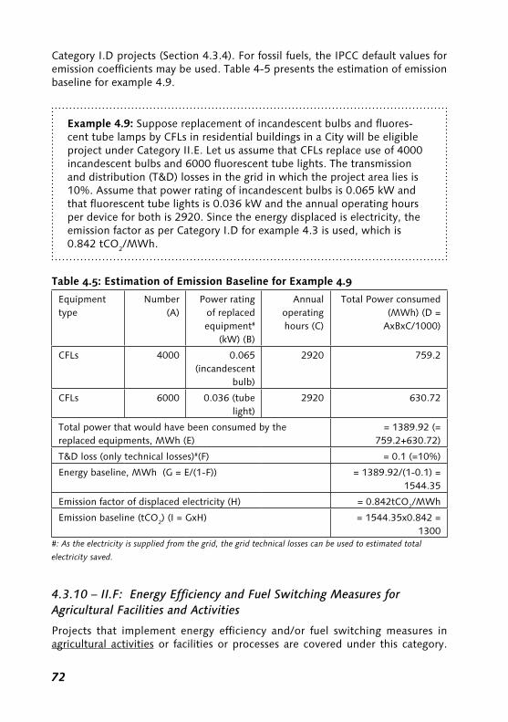
Category I.D projects (Section 4.3.4). For fossil fuels, the IPCC default values for emission coefficients may be used. Table 4-5 presents the estimation of emission baseline for example 4.9.

Example 4.9: Suppose replacement of incandescent bulbs and fluores-cent tube lamps by CFLs in residential buildings in a City will be eligible project under Category II.E. Let us assume that CFLs replace use of 4000 incandescent bulbs and 6000 fluorescent tube lights. The transmission and distribution (T&D) losses in the grid in which the project area lies is 10%. Assume that power rating of incandescent bulbs is 0.065 kW and that fluorescent tube lights is 0.036 kW and the annual operating hours per device for both is 2920. Since the energy displaced is electricity, the emission factor as per Category I.D for example 4.3 is used, which is 0.842 tCO2/MWh.

Table 4.5: Estimation of Emission Baseline for Example 4.9

Equipment type

Number (A)

Power rating of replaced equipment#

(kW) (B)

Annual operating hours (C)

Total Power consumed (MWh) (D =

AxBxC/1000)

CFLs 4000 0.065 (incandescent

bulb)

2920 759.2

CFLs 6000 0.036 (tube light)

2920 630.72

Total power that would have been consumed by the replaced equipments, MWh (E)

= 1389.92 (= 759.2+630.72)

T&D loss (only technical losses)#(F) = 0.1 (=10%)

Energy baseline, MWh (G = E/(1-F)) = 1389.92/(1-0.1) = 1544.35

Emission factor of displaced electricity (H) = 0.842tCO2/MWh

Emission baseline (tCO2) (I = GxH) = 1544.35x0.842 = 1300

#:Astheelectricityissuppliedfromthegrid,thegridtechnicallossescanbeusedtoestimatedtotal

electricitysaved.

4.3.10 – II.F: Energy Efficiency and Fuel Switching Measures for Agricultural Facilities and Activities

Projects that implement energy efficiency and/or fuel switching measures in agricultural activities or facilities or processes are covered under this category.

��

Examples of energy-efficient practices include efficiency measures for specific agricultural processes (such as decrease in irrigation used, etc.), and measures leading to a reduced requirement of farm power per unit area of land, reflected in lesser number of hours of tractor use or smaller capacity tractors, and less use of farm equipments. Further energy efficient measures would be reducing fuel use in agriculture, such as reduced machinery use through, e.g. the elimination of tillage operations, reduction of irrigation, use of lighter machinery, etc. Examples of fuel switching measures include switching from diesel to ethanol or biodiesel.

The projects could be either a replacement of existing equipment or installation of equipment in a new facility. The aggregate energy savings of a single project may not exceed the equivalent of 15 GWh per year.

Energy baseline

(a) Energy baseline in the case of retrofit measures would be expressed in terms of energy consumption of the existing activity that would be avoided; or

(b) In the case of a new facility the baseline would be expressed as energy con-sumption of the facility that would otherwise be installed.

If the project results in fossil fuel saving (reduced tillage activity implies lower tractor use and, hence, lower fossil fuel use) the energy baseline is the fossil fuel consumption of the baseline activity. The fuel consumption can be expressed as total fuel consumption for baseline activity or as a product of fuel consumption per unit area and total area under agricultural activity.

If the project results in savings in electricity (say, reduced water requirement implies lower use of electric pumps to irrigate and, hence, savings in electricity), the energy baseline is consumption of electricity by baseline activity divided by technical transmission and distribution losses for the electrical grid serving the agricultural facility.

The demonstration of additionality for projects under this category is necessary, especially with respect to some financial indicators. Also the project participants should clearly demonstrate that reduced energy consumption is not due to de-crease in the activity (say, decrease in cropped area) due to financial constraints faced by them, but is due to the CDM-driven activity.

Example 4.10: A proposed CDM project involves adoption of a no-tillage method of farming on 1000 hectares of agricultural land. Assume that an-nual operating hours of a tractor for tilling a hectare of land is 500 and a tractor consumes on average 10 kg of diesel per hour. Therefore, the total amount of diesel saved by adopting no-tillage method is 5,000 tonnes.

��

Energy and emission baseline for example 4.10 can be estimated as follows:

Energy baseline (A) = 5000 tonnes diesel

Emission factor for Diesel (B)

= 3.2 tCO2 /tonne diesel (IPCC default value)

Emission baseline (C = (A)x(B)

= 5000 tonnesx3.2 tCO2 /tonne diesel = 16,000 tCO2

4.3.11 – III .A: Agriculture

The CDM-EB is still to finalize the simplified baseline methodology for this category of projects.

4.3.12 – III.B: Switching Fossils Fuels

This category comprises fossil fuel switching in existing industrial, residential, com-mercial, and institutional or electricity generation applications. The fuel switching activity of the proposed project may change efficiency of the system as well. The primary focus of the project activity should be to reduce emissions through fuel switching. If fuel switching is a part of the project activity focused primarily on energy efficiency, the project activity falls in Category II.D (Section 4.3.8) or II.E (4.3.9).

Emission baseline

The emission baseline is the current emissions of the facility expressed as emis-sions per unit of output (e.g., kg CO2e/kWh). IPCC default values for emission coefficients may be used.

Example 4.11: Say, a proposed CDM project switches from fuel oil use to gas in reheating furnace in a steel re-rolling mill. Assume that existing annual fuel consumption of the steel mill is 6441.6 kiloliters (product of annual production (105,600 tonnes) and fuel intensity of production (61 liters fuel oil per tonne of output)). Say, the energy required per tonne of steel in gas furnace is 1866 MJ.

��

The emission baseline for example 4.11 can be estimated as follows:

Annual output of the mill (A) = 105,600 tonnes

Annual Fuel oil consumption (B) = 6441.6 kilo liters (5340 tonne)

Emission factor of Fuel Oil (tC/103 tonne) (C)

=848 (IPCC default for residual fuel oil)

Annual CO2 emissions (tonne) (D = BxCx44/12) = 0.848x5340x44/12 = 16604

Emission baseline (E = D/A) = 16604/105600 = 157 kgCO2/ tonne output

For the proposed CDM project to be eligible under SSC, total project emissions should be less than 15 kilotonne CO2. Since the estimated emission from project is less than 15 kilotonne CO2, as shown in calculations below, the project is eligible under SSC.

Annual output of the mill (A) = 105,600 tonne

Estimated Energy required per tonne of steel heated (B) = 1866 MJ/tonne

Estimated annual energy required (C = AxB) = 197.050 TJ

Emission factor of Gas (tC/TJ) (D) = 15.3 (IPCC default for residual fuel oil)

Estimated project CO2 emissions (tonne) (E = DxCx44/12) = 15.3x197.05x44/12 = 11056

4.3.13 – III.C: Emission Reductions by Low-Greenhouse Gas Emitting Vehicles

Projects aiming at reducing GHG emission through low-GHG emitting vehicles are included in this category. A project activity in this category should both re-duce anthropogenic emissions by sources and directly emit less than 15 kiloton-nes of carbon dioxide equivalent annually.

Emission baseline

The emission baseline is measured as product of the energy use per unit of service for the baseline vehicle (A), the average annual units of service per vehicle (B), the number of vehicles affected (C), and the emission coefficient for the fuel used by vehicle (D) that would have been used in absence of the project. Therefore, the emission baseline can be expressed as,

Emission baseline = AxBxCxD

If electricity is used by the vehicles, the associated emissions shall be estimated in

��

accordance with methodology category I.D project activities (Section 4.3.4).

Example 4.12: Say, a proposed CDM project involves use of ethanol to substitute 10% gasoline in a fleet of 1000 private cars. Assume that on average cars consume 0.1 litre of gasoline per km and the average annual travel is 10,000 km. Substitution of gasoline by ethanol does not result in any change in fuel use efficiency; therefore, the reduction in gasoline is equal to the amount of ethanol used in the cars.

The baseline for example 4.12 can be estimated as shown below.

Fuel consumption of a car per km (A) = 0.1 litre gasoline (0.074 kg)

Average annual distance traveled per car (B) = 10,000 km

Number of cars covered in the project (C) = 1000

Emission factor of gasoline(kgC/ tonne) (D) = 847 (IPCC default for gasoline)

Emission baseline (tonne CO2) (E = AxBxCxDx44/12)

= (0.074x10,000x1000x0.847)x 44/12 = 2298.2

Project emission (tonne CO2) = 0.9x2298.2 = 2068.4*

*:Inprojectcase�0%ofgasolineconsumptionisreplacedbyethanol,whichisproducedfromorganicsourcesandhaszero

GHGemissions.Therefore,only90%ofbaselinegasolineusedinbaselineresultsinemissionsduringprojectcase.

The calculations above show that project emissions are 2.07 kilotonne of CO2, which is less than the 15 kilotonnes value, hence, the project is an SSC project.

4.3.14 – III.D: Methane Recovery

This category includes projects that prevent release of methane emissions into the atmosphere from coal mines, agro-industries, landfills, wastewater treatment facilities and other sources through measures to recover the emitted methane. This category includes projects that process organic components of municipal solid waste prior to its disposal in a landfill site and reduces the potential for methane emissions. But projects that use the organic component of municipal solid waste for incineration to avoid methane emissions are not covered in this category. If the methane captured is from a non-biogenic source (methane captured in coal mines) then the CO2 emission from the combustion of captured methane is counted in project emissions.

��

Emission baseline

The emission baseline is defined as the amount of methane that would be emit-ted to the atmosphere in the absence of the proposed project activity. In the case where certain proportion of methane in the baseline is captured and flared, then it is also accounted for.

It should be noted that in the case of landfill gas, waste gas, waste water treatment and agro-industries projects, if recovered methane is used for electricity generation, the proposed project activity is also eligible under Category I.D (Section 4.3.4). If in a project, methane recovered is used for heat generation, the project is also eligible under Category I.C (Section 4.3.3). In such cases, project participants may submit one single project design document for all of the components of the proposed project activity.

Example 4.13: Suppose a proposed CDM project will install a gas recov-ery system in an existing landfill site, which daily receives 20,000 tonnes of waste (W). The captured gas will be used to generate electricity and supplied to the grid. The project will also install a flaring system to flare gas captured in excess of that used for generating electricity.

The gas capture component of the proposed project falls under category III.D, whereas, the use of gas to produce electricity component will fall under category 1.D. Project proponents can develop one single PDD for both these compo-nents.

The baseline (BE) for the project in example 4.13 is calculated using the IPCC recommended methane estimation method,13 as below:

BE = W x MFx 2114, and

MF = MCF x DOC x DOCF x F x 16/12

Methane Correction Factor (MCF) = 0.6 (IPCC Default)

DOC = 0.18 (IPCC Default)

DOCF = Fraction DOC dissimilated as landfill gas = 0.77 (IPCC Default)

F = fraction of CH4 in landfill gas = 0.5 (IPCC Default)

Methane factor for waste (MF) = (0.6x0.18x0.77x0.5) = 0.042

Baseline emission, BE = 20,000x0.042x21 = 17,640 tonnes

�3 SeeChapter“Waste”ofIPCCgreenhousegasNationalInventory:Workbookfordetailsofmethane

estimationfromsolidwastedisposal.

�4 GlobalWarmingPotential(GWP)ofmethane.

��

Assume that in example 4.13, 10% of methane generated during project phase will escape into atmosphere, that is, only 90% of the methane generated during project phase is captured.

Project emissions = 0.1x17,640 = 1764 tCO2e, since this is less than 15 kilo-tonne, the project is eligible as an SSC project. Also note that CO2 emission from flaring or burning the CH4 in generator is not accounted for because the source of gas is organic.

4.3.15 – III.E: Avoidance of Methane Production from Biomass Decay through Controlled Combustion Technology/Measures

This category includes project activities that avoid the production of methane from biomass or other organic matter, which otherwise would have been left to decay and emit methane. The methane emission is avoided by utilization of the biomass or organic matter for controlled combustion in the project scenario. The project activity here does not recover or combust methane (unlike Category III.D (Section 4.4.14)). For example, a project that uses the organic component of municipal solid waste for incineration to avoid methane emissions will be covered in this category.

Emission baseline

The baseline scenario is the situation where the biomass and other organic mat-ter would be left to decay within the project boundary resulting in generation of methane which would be emitted to the atmosphere. The baseline emission is the amount of methane generated from the decay of the biomass or organic waste that would be treated in the project activity. IPCC default emissions factors can be used. The baseline (BEy) can be estimated using as follows:15

BEy = Qbiomass x CH4_IPCCdecay x GWP_CH4

where,

Qbiomass Quantity of biomass treated under the project activity (tonnes)

CH4_IPCCdecay IPCC CH4 emission factor for decaying biomass in the region of the project activity (tonnes of CH4/tonne of biomass or organic waste)

GWP_CH4 GWP for CH4 (tonnes of CO2 equivalent/tonne of CH4)

�5 ThemethodissuggestedbyCDM-EB.

��

CH4_IPCCdecay = (MCF x DOC x DOCF x F x 16/12) where,

MCF methane correction factor expressed as fraction (default value of parameter as per IPCC is 0.4)

DOC degradable organic carbon expressed as fraction (IPCC default is 0.3)

DOCF fraction DOC dissimilated to landfill gas (IPCC default is 0.77)

F fraction of CH4 in landfill gas (IPCC default is 0.5)

DOC can also be estimated as follows:

DOC = 0.4 (A) + 0.17 (B) + 0.15 (C) + 0.30 (D)

where,

A per cent waste that is paper and textilesB per cent waste that is garden waste, park waste or other non-food

organic putresciblesC per cent waste that is food wasteD per cent waste that is wood or straw

Baseline emission should not include methane emissions captured and remo-ved to meet the national or local safety requirement or legal regulations. For example, if local or national safety regulations on landfill sites mandate capture and removal of 10% of methane, then the baseline would be only 90% of the methane emission, or

BEy = 0.9x Qbiomass x CH4_IPCCdecay x GWP_CH4

4.4 Submitting New Methodology and New Small Scale CDM Project Categories The suggested methodologies for small-scale CDM projects are not exhaustive. Project proponents can propose changes to the simplified baseline methodo-logies. Also, the project categories suggested do not imply that a small scale CDM project is ineligible if it does not fall under any of the existing categories. The project proponent can propose additional project categories for considera-tion by the CDM-EB. The project participants make a request to the CDM-EB providing information about the technology/activity and proposals on how a simplified baseline and monitoring methodology would be applied to this cate-

�0

gory. If the proposed methodology is approved by the CDM-EB, the approved methodology is added in the Appendix B of the modalities and procedures of the small-scale CDM project activities16.

�� TheExecutiveBoardwillreviewandamend,asnecessary,appendixBatleastonceayear.

AnyamendmentstoappendixBwillapplyonlytoprojectactivitiesregisteredsubsequenttothedateof

amendmentandshallnotaffectregisteredCDMprojectactivitiesduringthecreditingperiodsforwhich

theyareregistered.

��

Annex IV A: Default Carbon Emission Factor and Net Calorific Values as per IPCC (source: Revised 1996 IPCC guidelines for National Greenhouse Gas Inventories: Workbook, Table 1.2 &1.3, page 1.6 of Energy Section)

Table IV A-1: Carbon Emission Factors (CEFs)

Fuel Carbon Emission Factors (t C/TJ)

LIQUID FOSSIL

Primary Fuels

Crude Oil 20.0

Orimulsion 22.0

Natural Gas Liquids 17.2

Secondary Fuels/Products

Gasoline 18.9

Jet kerosene 19.5

Other Kerosene 19.6

Shale Oil 20.0

Gas/Diesel Oil 20.2

Residual Fuel Oil 21.1

LPG 17.2

Ethane 16.8

Naphtha (20.0) (a)

Bitumen 22.0

Lubricants (20.0) (a)

Petroleum Coke 27.5

Refinery Feedstocks (20.0) (a)

Refinery Gas 18.2 (b)

Other Oil (20.0) (a)

SOLID FOSSIL

Primary Fuels

Anthracite 26.8

Cooking coal 25.8

Other Bituminous Coal 25.8

Sub- bituminous Coal 26.2

Lignite 27.6

Oil Shale 29.1

Peat 28.9

��

Secondary Fuels/Products

BKB & Patent Fuel (25.8) (a)

Coke Oven/Gas Coke 29.5

Coke Oven Gas 13.0 (b)

Blast Furnace Gas 66.0 (b)

GASEOUS FOSSIL

Natural Gas (Dry) 15.3

BIOMASS

Solid Biomass 29.9

Liquid Biomass (20.0) (a)

Gas Biomass (30.6) (a)

(a)ThisvalueisadefaultvalueuntilafuelspecificCEFisdetermined.ForGasbiomass,theCEFis

basedontheassumptionthat50%oftheCarboninthebiomassisconvertedtomethaneand50%is

emittedasCO2.TheCO2emissionsfrombiogasshouldnotbeincludedinnationalinventories.Ifbiogas

isreleasedandnotcombusted50%ofthecarboncontentshouldbeincludedasmethane.

(b)Foruseinthesectoralcalculations.

Table IV A-1 (contd.)

��

Table IV A-2: Selected Net Calorific Values

Refined Petroleum Products Factors (TJ/103 tonnes)

Gasoline 44.80

Jet Kerosene 44.59

Other Kerosene 44.75

Shale Oil 36.00

Gas/Diesel Oil 43.33

Residual Fuel Oil 40.19

LPG 47.31

Ethane 47.49

Naphtha 45.01

Bitumen 40.19

Lubricants 40.19

Petroleum Coke 31.00

Refinery Feedstocks 44.80

Refinery Gas 48.15

Other Oil Products 40.19

Other Products

Coal Oils and Tars derived from Cooking Coals 28.00

Oil Shale 9.40

Orimulsion 27.50

��

Chapter V

Establishing baselines for large scale CDMprojects

This Chapter discusses establishing project-specific baselines for large scale CDM projects. As discussed in Chapter 2, baselines for proposed CDM projects should be established using a CDM-EB approved baseline methodology. A number of methodologies have already been approved by the CDM-EB. Project proponents can employ one of the approved methodologies (AM) applicable to their pro-jects to establish a baseline. However, if none of the approved methodologies are applicable to the proposed CDM project, the project proponents need to develop a new methodology for their project.

Figure 5.1: Procedure for establishing a baseline for a proposed CDM project.

Is any of the pre-approvedmethodology applicable to

proposed CDM project?

YesNo

Develop a NEWmethodology

Apply methodology to establish baseline

The chapter first discusses the use of pre-approved methodologies to establish the baseline. This is followed by a discussion on developing a new baseline methodology. The steps in using approved methodology and developing base-line methodology are explained with examples.

��

5.1 Establishing Baselines Using a Pre-approved Baseline Methodology (BM) A number of CDM-EB pre-approved methodologies are available for establishing project specific baseline at http://cdm.unfccc.int/methodologies/PAmethodo-logies/approved.html. Each approved methodology has two components, a baseline methodology (BM) and a monitoring methodology (MM). A BM con-tains five sections, viz., applicability, emission reduction, baseline, additionality, and leakage. In this section use of an AM in establishing a baseline is discussed. To demonstrate the use of an AM, components of an approved methodology AM0002 – “Greenhouse gas emission reductions through landfill gas capture and flaring where the baseline is established by a public concession contract”1 – is used. The relevant component of AM0002 is reproduced in boxes following the description of each step. The main steps for using of an approved methodo-logy are illustrated in Figure 5.2 and discussed below:

Figure 5.2: Steps for using approved baseline methodologies.

Step 1: Selection of AM from the list of existing AMs

Step 2: Justification of application of chosen AM to the Project using applicability conditions

Step 3: Using methodology provided in AM to assess additionality.

Step 4 Establishing Baseline

Step 5 Estimating Leakage

Step 6: Estimating Emission Reductions

Step 7: Preparing the Project Design Document for the Project.

Step 1: Identifying the appropriate approved methodology (AM)

From the list of AM methodologies which are for project types similar to a pro-posed CDM project, those likely to be applicable to the proposed CDM project are identified.

� Themethodologyisavailableoncdm.unfccc.intwebsite.

��

Step 2: Justifying application of chosen AM

Applicability of each identified AM is evaluated to identify the AM whose ap-plicability conditions are fulfilled by the proposed CDM project. Box 1 below gives an example of applicability conditions for the AM0002 methodology. The project proponents need to justify in the CDM-PDD why the chosen metho-dology is most appropriate for the proposed CDM project. The justification is provided by explaining how the proposed CDM project meets all the applicabi-lity conditions of the chosen AM.

BOX 1: Example of applicability conditions in AM0002

This methodology is applicable to landfill gas capture and flaring proj-ect activities where:

• There exists a contractual agreement that makes the operator responsible for all aspects of the landfill design, construction, operation, maintenance, and monitoring.

• The contract was awarded through a competitive bidding process.

• The contract stipulates the amount of landfill gas (expressed in cubic meters) to be collected and flared annually by the landfill operator.

• The stipulated amount of landfill gas to be flared reflects performance among the top 20%, of projects implemented in the previous five years for landfills, operating under similar social, economic, environmental and technological circumstances.

• Generation of electricity using captured landfill gas neither occurs nor is planned.

Step 3: Assessing additionality

The methodology provided in the identified AM is used to assess additionality of the proposed CDM project. The additionality assessment evaluates whether the proposed CDM project is a less likely option to be adopted vis-à-vis the baseline scenario. The baseline scenario is described in the baseline section of AM. The additionality section gives the factors and parameters to be used in undertaking the assessment. Box 2 gives an example of an additionality assessment using AM0002 methodology.

��

BOX 2: Additionality assessment in AM0002

The baseline scenario for the proposed project activity is the quantity of landfill gas (LFG) flared as determined by the contractual requirement, which is established through a competitive bidding process.

Project is additional if the actual quantity of methane flared is greater than the quantity of methane flared in the baseline scenario.

Further, to prove that the project activity is additional following should be demonstrated:

(i) Collection of LFG greater than that stated in the contract under the proposed CDM project results in additional costs, and

(ii) No additional revenues are expected from increased capture of LFG under the proposed CDM project.

Step 4: Establishing the baseline

Each AM has a section describing the baseline scenario as well as the formula used for estimating the baseline. The description includes definitions of the variables and parameters as well as sources of the data required for estimating baseline. Box 3 gives an example of baseline estimation for AM0002. The para-meter values used for estimating the baseline should be easily verifiable; that is, the source should be clearly stated and their use should result in a conservative estimate of the baseline.

Box 3: Baseline for AM0002

The baseline scenario is capture and flaring of LFG as stated in the CONTRACT. The remaining LFG produced in landfill is not captured and thus released into the atmosphere. The contract also specifies the quan-tity of waste projected to be disposed at the landfill during each year (WASTEcontract,y).

The baseline is the amount of methane flared each year (CH4contract,y), which is the product of the quantity of LFG required to be flared as per the contract and an appropriate methane content per unit LFG factor to give a conservative baseline.

��

Box 3 continued

The quantity of methane projected to be generated during a given year (CH4projected,y) is

CH4projected,y = k x L0 x ∑t=0,y WASTEcontract,t x e-k(t-y)

Where L0 is the methane generation rate (Nm3/tonne WASTE) and k is the decay rate. These factors are site specific and will be chosen by users of the methodology.

The projection of quantity of landfill gas to be generated during a given year (LFGprojected,y)is.

LFGprojected,y = CH4projected,y /(CH4/LFGcontract)

CH4/LFGcontract is the methane content of the landfill gas, assumed by the contract.

The quantity of methane required to be flared during each year (CH4contract,y) as specified in the contract is calculated as follows:

CH4contract,y = (LFGprojected,y x CH4/LFGcontract )x FDy

Where, FDy is the contract specified fraction of LFG captured and flared.

If the actual waste disposed is different from that specified in the con-tract, The baseline quantity of methane flared (CH4baseline,y) is adjusted as the following formulae:

CH4baseline,y = CH4contract,y x (WASTEactual,y/WASTEcontract,y) x ([CH4/LFGactual]/[CH4/LFGcontract])

Step 5: Estimating leakage

The leakage from the project is estimated using the leakage formulae given in the identified AM. The source of data and method of estimating used in leakage formulae should be clearly mentioned in the document. Box 4 gives the leakage estimation method for AM0002.

��

BOX 4: Leakage estimation in AM0002

Leakage in the case of methodology is defined as emissions resulting from generating the excess electricity used, above that used in the baseline scenario, to pump the LFG in the collection equipment. The emissions (EEy) are

EEy= [(CH4flared,y – CH4baseline,y)/CH4baseline,y] x EPy x ECy/1000

EPy: metered electricity use by the pumping equipment in kWh

ECy: emissions coefficient for the electricity used measured in kg CO2e/kWh. The emissions coefficient should be estimated using an appropriate methodology given the source of the electricity supply.

Step 6 – Estimating emission reductions

The generic formula for estimating the emission reduction (ER) from the pro-posed project is:

ER = Baseline – Project emissions – Leakage

The identified AM provides the formula for ER as well as estimating the project emissions. Box 5 gives the ER estimation procedure for AM0002. Note that though the estimation of emission reduction for issuance of CERs will be based on the monitored value of project emissions and leakage, the CDM-PDD should include the estimated emission reduction from proposed project based on esti-mated amount of project emissions and leakage.

BOX 5: Emission reduction estimation method in AM0002

The GHG emission reduction (ERy) by the proposed project activity for a year (y) is equal to the methane emission reduction (ER_CH4y) during that year multiplied by a conversion factor (CF) and by the approved Global Warming Potential value for methane (GWP_CH4).

ERy = ER_CH4y x CF x GWP_CH4

The conversion factor (CF) is the tonnes of methane per cubic metre of methane at standard temperature and pressure (0.000662 tonnes CH4/m3). The approved Global Warming Potential value for methane for the first commitment period is 21 tonnes CO2e/tonne CH4.

�0

Box 5 continued

ER_CH4y= CH4flared,y – CH4baseline,y

CH4flared,y is determined by monitoring the quantity of methane actually flared using the approved monitoring methodology. CH4flared,y is measured in cubic metres (Nm3).

STEP 7 – Completing the CDM-PDD

The project proponents should present information on project details and the sector situation in which the project is located (in Section A of CDM-PDD) along with the details of the application of methodology (Section B and Section E of CDM-PDD) in the CDM-PDD. The details provided in Section A of CDM –PDD support the justification for the application of a methodology as well as the appropriateness of the baseline scenario stated in the AM in the context of the proposed project. The CDM-PDD should include the references to all docu-ments from which information has been used to justify the assumptions and source data.

Any deviations from the method described in the AM would be considered as a new methodology and, hence, would have to be approved by the CDM-EB prior to use. For example, AM0002 is used for a landfill project, which though meeting all the applicability conditions mentioned in Box 1, has also to comply with a new environmental regulation. Say the environment regulation requires flaring of a higher quantity of LFG in the baseline than stated in the contract. This implies that a correction factor has to be applied to the formula for estima-ting the baseline to capture the impact of the environmental regulation. If such a change is made to the formula then the methodology will be treated as a new methodology.

In many cases a proposed CDM project might not meet all the applicability conditions of an AM, but is very similar to the project type for which the AM is proposed. In such cases, project proponents could use the AM and modify it to incorporate the special feature of their proposed project. This will reduce the time required for developing a new methodology.

5.2 Developing a New Baseline MethodologyIn the absence of an AM applicable to the proposed project, a new BM has to be developed. The example of AM0002 in Section 5.1 highlights the impor-tant elements of a BM. Though a new BM is developed with a specific project

��

in mind, the description of a BM and its use to establish the baseline are two different activities. The BM describes the process of or steps taken in establish-ing the baseline and estimating emissions reductions. These steps are described in the prescribed format for submission of new BM (CDM New Methodology Baseline: CDM-NMB).2

The application of a BM to the specific project for which it has been developed is described in the CDM-PDD3. To illustrate the difference, the BM could be compared to a set of mathematical equations to estimate the volume of any container and will be described in CDM-NMB, whereas, the application of the equations in the context of a particular container is akin to establishing a base-line for a specific project and is described in the CDM-PDD.

Figure 5.3 – Steps in developing a new baseline methodology.

Step 1: Identifying the GHG impact

Step 2: Defining the project boundary

Step 3: Identifying alternative Baseline Scenarios

Step 4: Assessing additionality of proposed CDM project

Step 5: Identifying the Baseline scenario and the baseline approach

Step 6: Developing methodology for estimating Baseline emissions

Step 7: Assessing Leakage from project and Formulae to estimate leakage

Step 8: Developing methodology for assessing Project Emissions and Emissions reduction

Step 9: Assessment of Robustness of BM – key assumptions and uncertainty

Step 10: Completing CDM-NMB and CDM-PDD

2 Thedocumentisavailableathttp://cdm.unfccc.int/Reference/Documents/cdm_nmb/English/CDM_

NMB.doc.PreviouslythenewbaselinemethodologywasdescribedinAnnex3oftheCDM-PDD.

3 Thedocumentisavailableathttp://cdm.unfccc.int/Reference/Documents/cdmpdd/English/CDM_

PDD_ver02.doc.

��

Figure 5.3 presents the steps to develop a new BM (NBM). The process of developing an NBM is not as linear as represented in the figure. The process is iterative as the different steps in the processes have significant informational interdependence.

The different steps in developing a new baseline methodology are demonstrated through their application to an example of developing the NBM for waste gas based power generation project (described in Box 6).

Box 6 – Description of an example project, the Waste Gas Utilization Project

The proposed CDM project uses the excess CO rich waste gas, gener-ated in the process of steel making, to generate electricity. The project will be implemented in an existing steel plant. Waste gas has a significant combustible proportion of CO resulting in a gross calorific value of 2000 kilo calories per NM3 (m3 measured at normal temperature and pressure conditions). The gas will be used by the project proponents to partially reduce the coal consumed in generating electricity from an existing cap-tive power plant. Presently the waste gas generated is partially used for meeting heating requirements within the steel plant and the remaining gas is flared.

5.2.1 Identifying the GHG Impact

The baseline describes the emissions from sources that are affected by the im-plementation of the proposed CDM project. Therefore, the first step in develo-ping an NBM is to clearly identify the action or activity of project that affects the GHG emissions, the GHG impact of project. If there are more than one GHG impacts of the project, then each impact would require a separate NBM. For example, a project to capture LFG and use it to generate electricity for supplying to the grid has two GHG impacts. One, it will reduce emissions from avoided re-lease of LFG into the atmosphere, and two, will reduce emissions from displace-ment of electricity generated from a fossil fuel based generation source supply-ing the grid. The project proponents can use CDM-EB approved “consolidated methodology for landfill gas projects (ACM0001)”,4 but only to establish the baseline for the first GHG impact. The baseline for the second GHG impact can be established using “consolidated methodology for grid-connected electricity

4 Themethodologyisavailableathttp://cdm.unfccc.int/methodologies/PAmethodologies/approved.

html

��

generation from renewable sources (ACM0002)”5. Box 7 presents identification of GHG impact for the example project.

Box 7 – Identification of GHG impact in the Waste Gas Utilization Project

The proposed CDM project will use waste gas to generate electricity. The GHG impact will depend on different possibilities for using waste gas to generate electricity, which are:

(i) Use of waste gas in the steel plants’ captive power plant (excess generation is supplied to the grid). Waste gas will replace a part of the current fuel, coal. – The GHG impact in this case is from reduction in coal consumption of the captive power plant.

(ii) Use of waste gas as fuel along with coal in a planned captive power generation plant for the steel plant. The electricity is presently purchased from the grid. – The GHG impact in this case is from reduction of coal consumption due to use of waste gas.

(iii) Use of waste gas to meet the fuel requirements for capacity expansion of an existing captive generation plant. Capacity expansion will enable the electricity requirement of the steel plant, which is presently met by the grid, to be met using waste gas. The expanded capacity based solely on waste gas can be treated as a new facility and displaces electricity from existing generation facilities that supply the grid. – The GHG impact in this case is the reduced emission from existing generating sources that supply the grid or will be added to the grid in future.

(iv) Use of waste gas as the sole fuel in a grid connected new generation plant – the GHG impact in this case is reduced emissions from existing generation sources supplying to the grid or will be added to the grid in the future.

As mentioned in Box 6, the waste gas will be used to replace partially the coal used in an existing captive power plant without any expansion of the capacity. Therefore, the GHG impact of the project is from reduction in emissions due to the decrease in the use of coal.

As can be seen from the Box 7, the identification of GHG impact also identifies

5 Themethodologyisavailableathttp://cdm.unfccc.int/methodologies/PAmethodologies/approved.

html

��

Box A: On-site and off-site emissions

For a CDM project to replace coal by natural gas in an industrial complex the direct and indirect on-site emissions as well as direct and indirect off-site emissions are:

Direct on site

GHGs emission from natural gas use in the project scenario.

GHGs emission due to fuel consumption by fuel handling facilities or equipment.

Indirect on site

Emission from construction or installation of natural gas in the project scenario.

Off-site emissions refer to emissions outside the physical boundary of the project. In the above example of a coal-to-gas CDM project, the direct and indirect off-site emissions could include the following.

Direct Off Site

Emission of all types of GHGs from natural gas transportation (i.e., pipe-line) in the project scenario. This mainly includes emissions resulting from fuel (gas or electricity) consumption by the pipeline. It, however, entirely depends on the project-specific situation to decide which emissions should be included and how these are to be estimated. For example, if the gas consumption is a small fraction of total gas transported (either daily or annually) through the pipeline, the emissions related to the pipeline may not be included in the CDM project-related emissions. On the other hand, if the pipeline is built solely to transport gas to the CDM project, emissions related to the transportation are accounted for in the CDM project.

Indirect Off Site

Emissions for construction of a gas pipeline if the pipeline is built solely for transporting gas to the CDM project.

the GHG sources that will be affected by the proposed CDM project. This is important in developing the baseline scenario.

5.2.2 Defining Project Boundaries

The project boundary of a CDM project activity encompasses all anthropogenic emissions by sources of GHGs under the control of the project participants that are significant and reasonably attributable to the CDM project activity. Proj-ect boundaries vary across the project types. A project boundary is defined to identify all sources of GHGs that are affected by the project activities and com-pare the emissions in the baseline scenario to estimated emissions reductions achieved by the project.

The elements of a project boundary include the following:

1. All the emissions sources whose emissions are attributable to CDM project activity.

2. Anthropogenic emissions of six GHGs (i.e., CO2, N2O, CH4, HFCs, PFCs, SF6) from sources within the project boundary that would be directly or indirectly affected by project activities.

Some of the terms employed in defining the effect of project activities on GHG emissions by methodologies submitted to the CDM-EB, which were subse-quently approved, are: direct on-site emissions; in-direct on-site emissions; direct off-site emissions; and indirect off-site emissions. However, these classifi-cations are not mentioned in either the guidelines of the M&P for CDM or the text of the approved methodologies prepared by the CDM-EB.

On-site loosely refers to the physical boundary of the project facilities. The emissions directly affected are referred to as DirectOn-site emissions and the emissions indirectly affected are referred to as IndirectOnSite emissions. Box A explains these terms and illustrates them with an example. These demarcations are used as a tool to define the project boundary. Appendix V A gives some examples of these demarcations from the approved methodologies.

The project boundary could be the physical boundary of a proposed CDM project or also include the physical boundary of sites that result in changes in GHG emissions due to implementation of a project and are directly controlled by proponents of the proposed CDM project. The first step in identifying the project boundary is a diagrammatic representation of the project activity within the physical boundary of the project, processes upstream and downstream con-nected to the project, and facilities supplying services similar to the proposed CDM project to the same market (Figure 5.4). The upstream activities of a project could be linked through supply of energy, inputs, etc. The downstream industry represents industry consuming the output from the project. Emissions

��

the GHG sources that will be affected by the proposed CDM project. This is important in developing the baseline scenario.

5.2.2 Defining Project Boundaries

The project boundary of a CDM project activity encompasses all anthropogenic emissions by sources of GHGs under the control of the project participants that are significant and reasonably attributable to the CDM project activity. Proj-ect boundaries vary across the project types. A project boundary is defined to identify all sources of GHGs that are affected by the project activities and com-pare the emissions in the baseline scenario to estimated emissions reductions achieved by the project.

The elements of a project boundary include the following:

1. All the emissions sources whose emissions are attributable to CDM project activity.

2. Anthropogenic emissions of six GHGs (i.e., CO2, N2O, CH4, HFCs, PFCs, SF6) from sources within the project boundary that would be directly or indirectly affected by project activities.

Some of the terms employed in defining the effect of project activities on GHG emissions by methodologies submitted to the CDM-EB, which were subse-quently approved, are: direct on-site emissions; in-direct on-site emissions; direct off-site emissions; and indirect off-site emissions. However, these classifi-cations are not mentioned in either the guidelines of the M&P for CDM or the text of the approved methodologies prepared by the CDM-EB.

On-site loosely refers to the physical boundary of the project facilities. The emissions directly affected are referred to as DirectOn-site emissions and the emissions indirectly affected are referred to as IndirectOnSite emissions. Box A explains these terms and illustrates them with an example. These demarcations are used as a tool to define the project boundary. Appendix V A gives some examples of these demarcations from the approved methodologies.

The project boundary could be the physical boundary of a proposed CDM project or also include the physical boundary of sites that result in changes in GHG emissions due to implementation of a project and are directly controlled by proponents of the proposed CDM project. The first step in identifying the project boundary is a diagrammatic representation of the project activity within the physical boundary of the project, processes upstream and downstream con-nected to the project, and facilities supplying services similar to the proposed CDM project to the same market (Figure 5.4). The upstream activities of a project could be linked through supply of energy, inputs, etc. The downstream industry represents industry consuming the output from the project. Emissions

��

that are affected by the project activity in the four boxes (shown in Figure 5.4) are identified. Boundary covering all the sources of emissions affected due to the proposed CDM project that are under the control of proposed CDM project proponents are included in the project boundary.

Figure 5.4: Boundaries of CDM project activities.

Physical boundaryof the proposedCDM project

Upstreamactivitiesconnected to theProject

DownstreamActivities connectedto Project or ENDusers of projectservices.

Other supplier of same output asthe Project

For example, a proposed CDM project changes the process used for producing a commodity. The change in process results in increased consumption of an input that is produced at a facility under control of the project proponents but at a physically different location. Increased GHG emissions from increased produc-tion of the input should be included as project emissions. Therefore, the project boundary will be defined as the physical boundary of the proposed CDM project as well as the input producing facility (Figure 5.4A).

Figure 5.4 A: Project boundary if input production in separate facility is un-der the control of project proponents.

OutputProcess Change

CDM project(Physical

boundary ofproject)

Upstreamactivities

connectedto theProject

DownstreamActivities

connected toProject Or EndUsers of Project

services.

Upstream activity: Inputproduction unit under Project

proponent‘ssupplying input

to proposed CDM project

Other supplier ofsame output as

the Projectcontrol

��

The project boundary also helps identify the leakage. If the proposed CDM project results in an increase in emissions outside the project boundary which is measurable and directly attributable to proposed CDM project activity, the incremental emissions are termed as leakage. In the example discussed in the paragraph above, if the input producing facility is not under the management of project proponents of a proposed CDM project, the increase in emissions will be treated as leakage. The project boundary in this case is the physical boundary of the proposed CDM project (Figure 5.4B).

Figure 5.4B: Boundaries if input production facility not owned by project proponents.

OutputProcess Change

CDM project(Physical

boundary ofproject)

Upstreamactivities

connectedto theProject

DownstreamActivities

connected toProject Or EndUsers of Project

services.

Upstream activity: Inputproduction unit under Project

proponent‘ssupplying input

to proposed CDM project

Other supplier ofsame output as

the Projectcontrol

The term systemboundary has been used in some of the methodologies sub-mitted for approval to CDM-EB. The system boundary is essentially used to define the geographical scope or sectoral scope for the emissions sources to be considered in the baseline. For example, the GHG impact of a renewable based grid connected power generation project will be a reduction in emissions from existing generation sources connected to the grid. The system boundary defines the geographical expanse of the grid system to identify the generation sources that would emit GHGs in the absence of the proposed project.

Definitions of project boundary contained in already approved baseline metho-dologies are useful in understanding project boundaries. Table 5-1 summarizes the project boundaries defined in the baseline methodologies already approved by the CDM-EB.

��

Table 5-1: Examples of System Boundaries in Approved Baseline Methodologies

Approved Baseline Methodology

Definition of Project/system Boundary

NM0001 (AM0015): Vale do Rosario Bagasse Cogeneration (VRBC) Project, Brazil: Supply of electricity generated from surplus bagasse using higher efficiency boiler to the grid.

Baseline energy generation plants: The baseline boundary considers individual power plants connected to the grid.Bagasse cogeneration plant: The project boundary includes

the entire project site where the project activity will be implemented, that is, the bagasse electricity cogeneration project activity site, including all electrical generation equipments.

NM0010 (AM0010): Durban landfill-gas-to-electricity project, South Africa: The project uses the LFG gas captured from existing land fill site, which is otherwise being released to atmosphere, for generation of electricity, which is partially used on site and balance sold to the grid.

The physical boundaries includes landfill gas production from the landfills through production and safety wells, landfill gas collection using gas pumps and pipelines, landfill gas flaring, and combustion of landfill gas in engines and electricity generation units for on-site consumption and for sale to the grid. Since the electricity generated from the project is fed into the South African integrated electricity system, the system boundary includes the national power grid. South Africa grid is interconnected to neighbouring countries, but South Africa is a net exporter of power with unused excess capacity. Therefore, project’s additional generation capacity effects only power generation in South Africa and, hence, the relevant system boundary does not include the interconnection to the neighbouring countries.

NM0021 (AM0011): CERUPT Methodology for Landfill Gas Recovery: The project captures the LFG gas from existing landfill site, which was otherwise released into atmosphere, and used to generate electricity for on-site use.

The system boundary includes emission related to project site only.

NM0007 (AM0001): Incineration of HFC 23 Waste Streams from HCFC production facilities, Korea

The project boundary is defined as the facility to decompose the HFCs in the HCFC 22 production facilities.

NM0016 (AM0008): Graneros plant fuel switching project, Chile – Switch from coal to Natural gas as main fuel for milk products industrial unit.

The system boundary includes all types of GHG emissions from the plant site, emissions from coal mining and transportation even for coal imported from other Non-Annex I countries.

NM0023 (AM0023): Mexico- El Gallo hydro power Project

The system boundary includes Mexico’s national power grid.

��

Box 8: Defining the project boundary for the Waste Gas Utilization Project

The proposed project uses the excess waste gas to partially replace use of coal in the captive power plant. The excess waste gas is presently flared. Because waste gas generation is not uniform, the project will construct a collection network and storage system for the waste gas. The waste gas supply to the power plant will be regulated from the collection tank. Booster pumps will be installed to pump gas from storage tank to the power plant. Presently a part of the waste gas is used within the steel plants as a fuel for heat supply. Figure B8-1 gives the existing schematic of production process.

Figure B8-1: Schematic of existing situation at steel plant.

Electricity

Power Plant

CoalCoal

WasteGas

HeatFossilFuel

Waste Gasgeneration

sources

Heatgeneration

system

Generationunit

Coalhandlingfacility

CO2

CO2

CO2

Excess Waste Flare

The existing sources of emission are heat generation system (HGS), excess waste gas flaring and power plant. As only excess gas is used for power generation, the proposed CDM project will affect only two emissions sources– excess waste gas flaring and the power plant (see Figure B8-2). Further, a portion of the project waste gas will be used for pumping waste gas to the power plant.

�00

Figure B8-2: Proposed CDM project schematic.

Electricity

Power Plant

CoalCoal

BOFGas

HeatFossilFuel

Waste Gasgeneration

sources

Heatgeneration

system

Generationunit

Coalhandlingfacility

Fossil

fuel

CO2

CO2

Gas Storage& Pumping

CO2

The project boundary could be drawn excluding the HGS, as the HGS is not af-fected by project, unless the waste gas that could be used in the baseline in HGS is diverted to the power plant. In such a situation the proposed CDM project will also affect emissions from HGS.

5.2.3 Identifying Baseline Scenarios

The baseline is the scenario that reasonably represents the anthropogenic emissions by sources of GHG that would occur in the absence of the proposed project activity.6 In simpler terms, it constitutes the emissions from sources that are impacted by proposed CDM projects, if the project were not implemented. Therefore, the baseline scenario (BS) represents the existing GHG emission sources in the absence of a proposed CDM project. Since it is difficult to pre-cisely state what would happen in the absence of a proposed CDM project, different scenarios may be elaborated as a potential situation existing in absence of a proposed CDM project activity. The continuation of a current activity could be one of them; implementing the proposed project activity may be another; and, many others could be envisaged. Baseline methodologies should include a narrative description of all reasonable BS possibilities. Step 1 of the additionality tool (discussed in Chapter 3) also describes the process of identifying alternative BSs.

A good starting point for identifying the alternative BSs is the existing situation in the sector of the proposed CDM project. The use of technology/process, for

� PleaseseeAnnex4oftheMethodologyPanel’s�0thMeetingforfurtherclarificationonbaseline

scenario.

�0�

the activity proposed under the CDM project in the sector highlights the differ-ent options and possibilities. This also helps in defining the system boundary for the baseline scenario.

The scenarios should also be discussed in light of sectoral and national policies and circumstances, ongoing technological improvements, barriers, etc. The poli-cies/regulations/programs that should be considered in identifying alternative baselines scenarios are:

(i) Policies that affect relative fuel prices, e.g., duties on different fuels or removing restriction on import of a fuel, etc.

(ii) Policies that affect availability of finance for technologies, e.g., subsi-dies for renewable energy technologies.

(iii) Policies that affect competitiveness in the sector, e.g., making imports less restrictive.

(iv) Policies on import of technologies.

Figure 5.5: Identifying baseline scenarios.

Baseline Scenario1

Baseline Scenario3

Baseline Scenario2

Baseline Scenario4

Baseline Scenario2

Baseline Scenario

3

Baseline Scenario5

Baseline Scenario5

El iminate options that are either obsolete,not compatible with regulations, or otherreasons. Say, baseline scenario 1 and 4 are

screened.

Identify BaselineScenario

(Section 5.2.5)

�0�

(v) Infrastructural projects that influence fuel availability in the region.

(vi) Programs for demonstrating technologies and providing access to finan-cial resources for advanced technologies, e.g., a government program for modernization of a particular industry to improve its competitive-ness in the world economy.

(vii) Environmental regulations, such as emissions norms, zoning regula-tions, etc.

(viii) Specific regulations on energy efficiency standards or norms.

The CDM-EB has clarified that only those policies, regulations, and sectoral programs which favor more emission intensive activities can be considered in identifying alternative BSs that were implemented prior to 11th December 1997.

The policies/programs/regulations provide a basis for initial screening of possible BSs.

From the list of all possible scenarios, eliminate those which : (a) represent obsolete options (for example, though some cement plants in a county still use the wet process for producing cement, as no new plants using the wet process have been added in last many years, the wet process is not a plausible scenario); (b) will not meet the regulatory requirements (for example, if emission norms for power plants prohibit use of coal, then coal can not be considered as a base-line fuel option for generating power). Figure 5.5 illustrates steps in identifying alternative baseline scenarios. Box 9 presents the identification of BSs for the example project.

Box 9: Identifying alternative baseline scenarios for the Waste Gas Utilization Project

The GHG impact is from use of excess waste gas to produce electricity. Therefore, the starting point for developing alternative BSs is analysis of waste gas use in the steel industry in the country. The country could be the system boundary for setting the baseline for use of waste gas, but if there are distinct regional differences due to raw material or other inputs, then the region could be the system boundary. The possible options for use of waste gas are:

(i) x % of waste gas is used in steel plant for meeting heat require-ments and flaring of excess waste gas (100-x)%.

�0�

Box 9 (contd.)

(ii) Increase the percentage use of waste gas in the steel plant for heat requirement to the maximum feasible use (x1>x%) and the excess gas is flared (100-x1)%.

(iii) Use of excess waste gas in a captive power generation plant to par-tially replace the coal used.

(iv) Supply of the excess waste gas to other industries to meet the heat requirements of those industries.

The industry norm of waste gas use for heat requirement is the maximum feasible use (x1%), which is greater than the existing use of waste gas in the steel plant under consideration. Therefore, the first scenario is dis-carded as internal use of waste gas for heat purposes can increase to x1%.

Regulation on use of waste gas could also influence the percentage of waste gas use. Say there are no regulations for use of waste gas in the country.

Regulation on emissions from steel plant or the captive power plant too could affect the use of waste gas, if use of waste gas helps meet the emissions norms. If there were such a regulation, then one of the alterna-tive scenarios that should be considered is continued flaring of waste gas along with use of emission control equipments to meet the emissions regulation. Say the existing emission norms are met by the steel unit and power plant even when excess waste gas is flared.

5.2.4 Assessment of Project Additionality

As discussed in Chapter 3, assessment of additionality should clearly show that

(i) The project emissions (sequestrations) are less (greater) than the baseline emissions (sequestrations).

(ii) The proposed project should not be a baseline option, i.e., compared to the identified alternative BS the proposed CDM project is the least likely.

The CDM-EB recommended tool for assessment of additionality was discussed in detail in Chapter 3 to highlight the key elements of an additionality assess-ment. To illustrate the use of the tool, Box 10 presents the application of the tool to the waste gas utilization project.

�0�

Box 10 – Assessment of additionality in the Waste Gas Utilization Project using the CDM recommended tool.

Step 0 – This step is not applicable to the proposed project, as the project proponents will claim CER credits starting from registration of the project.

Step 1 – See Box 9 for identification of alternative baselines scenarios. As discussed in Box 9, the identified alternative baseline scenarios are: (i) the proposed project; and (ii) continued flaring of waste gas and purchase of electricity from the grid.

Step 2 – The level of investment in the alternative baseline scenario, continuation of present practice, is zero and, therefore, is not of the same order as that for the proposed CDM project. Therefore, a benchmark analysis (option iii) is chosen as a basis for analysis.

Say the financial indicator chosen for undertaking benchmark analysis is IRR on equity (since it is power project cost per unit of power delivered on the grid too could be used as the financial indicator). The benchmark chosen for comparison is government bond rates. Since the government bond rates represent risk free rates, the bond rate is adjusted with a risk premium to account for investment risk. Since the return on equity is being estimated, the expected return on stock market and risk premium factor for the stock market is used to adjust the government rates as per the following formulae:

Benchmark rate = Bond rate + risk factor x Equity market risk premium (EMRP)

EMRP is extra return stock markets provide over the safe rate of return.

As option iii is chosen, only the IRR estimate for the proposed CDM project activity is calculated and is compared to the benchmark return on equity. The following table presents the data that would be required to estimate the IRR of the proposed project.

�0�

Income/cost heads Yr0 Yr1 Yr2 Yr3 Yr last

Equity (E)

Revenue Fuel saving

Access electricity charge for renewable

energy

All Costs

Interest repayment

Gross Profit = all revenue minus costs & interest payment (GP)

Depreciation (D)

Profit less depreciation (GP-D)

Tax on (GP-D) = T

Tax breaks t

Net Profit = GP- (T-t)

Loan repayment (L)

Cash surplus (GP-T-L) = CS

0 = -E +∑(CS/(1+IRR)i

Summation is over the number of years (30). The solution to above equa-tion gives IRR for the proposed project. Say the project IRR is less than the benchmark value and, therefore, the proposed waste gas utilization project is not financially attractive.

The critical parameters in the financial analysis for the proposed project are: cost of coal saved, O&M cost of gas collection and supply system, estimate of benchmark IRR.

The possible range of values for these parameters are chosen and two sets of analysis carried out, viz., for extreme value of each critical parameter that results in a higher IRR and extreme value of each critical parameter that results in a lower IRR.

Say a high estimate of project IRR is less than the lower estimate of the benchmark; therefore, the project is unlikely to be financially attractive.

Box 10 (contd)

�0�

The next step in additionality assessment is Step 4, the Common Practice Analysis. If the project proponents like, they can also undertake Step 3, the Barrier Analysis. Since the investment analysis clearly demonstrates that the proposed project is not financially attractive, it is not necessary to conduct Step 3, the barrier analysis.

Step 4 – Say, the survey indicates that waste gas is utilized in the industry for heating purposes, but to a limited extent, and the remaining excess gas is flared. There exist a few projects that use waste gas to generate power. These projects were established under a demonstration program funded by an international donor. The proposed project does not receive the benefits received by the existing projects. Also, a few new projects are under implementation, but all these are being developed under CDM.

The proposed project is thus additional.

Step 5 – The non-viability of the proposed CDM project stems from three aspects: lower debt available requiring higher internal accruals/higher cost fund sources to meet the project cost; a higher interest rate on debt compared to other conventional projects; and, a shorter repayment schedule. These three factors combined decrease the IRR of the project. The CDM project revenues help access to greater debt at easier terms, as the total revenue stream of projects increases. The availability of greater debt with better terms lowers the cost of funds and thus improves the IRR even without the CER revenue. Inclusion of CER revenue further improves the IRR.

Therefore, the CDM impact on project improves its acceptability and, hence, the project is additional and, therefore, can not be considered as an alternative for the baseline scenario.

5.2.5 Baseline Approach and Baseline Scenario

Baseline approach defines the method of choosing the baseline scenario from the alternative baseline scenarios identified in the earlier step. The additionality assessment only proves whether the proposed CDM project is least likely com-pared to other identified alternative BSs.

For example, there may be only two alternative baseline scenarios, viz., conti-nuation of the existing practice and the proposed CDM project activity. Say the financial analysis shows that the proposed CDM project is financially less at-tractive than the existing practice. Therefore, the only possible baseline scenario

Box 10 (contd)

�0�

is continuation of past practice and the baseline approach is Approach A (as defined in Chapter 2, Section 2.3.2). On the other hand, for a case where there are more than two alternative baseline scenarios including the proposed CDM project, say the barrier analysis indicates that there are barriers that prevent implementation of the proposed CDM project but do not affect the other two alternatives. Then, the proposed CDM project is additional, and not a BS alter-native. Of the remaining alternative BSs, if the BS for the project is identified using financial/economic analysis, then the baseline approach is Approach B. But if none of the remaining BSs can be shown to be economically/financially most likely, and the baseline could be chosen as a weighted average of emissions under each alternative BS, then the approach is Approach C.

The baseline approach is linked to the formulae for estimation of the baseline. For Approach A, the baseline is emission from continuation of past practices. In Approach B, the baseline is emission from the most economically/financially attractive BS alternative. Table 5-2 lists the baseline approach used by different methodologies submitted to CDM-EB. Box 11 discusses the identification of baseline approach for the example project.

Table 5-2: Examples of Choosing BM Approaches from CDM M&P

BM Approaches chosen from CDM M&P Already approved BM choosing the Approach

Approach A: Existing actual or historical emissions, as applicable

HFC 23 destruction (AM0001); Fuel switching (AM0008); Methane from waste (AM0012, AM0013); Natural gas Cogeneration (AM0014); Baggase based cogeneration (AM0015)

Approach B: emissions from a technology that represents an economically attractive course of action, taking into account barriers to investment emissions, as applicable

LFG capture (AM0002, AM0003, AM0010, AM0011); Biomass power(AM0004); Hydro power (AM0005); Methane reduction from manure management (AM0006); Fuel switch (AM0007); Flared gas capture (AM0009);

Approach C: The average emissions of similar project activities undertaken in the previous five years and whose performance is among the top 20 per cent

None of already approved BM has chosen this approach, but some proposed BM have done so (e.g., NM0034).

*AMreferstoApprovedmethodologyandtheassociatednumbertothenumberofapprovedmethodology.

�0�

Box 11: Baseline approach for the Waste Gas Utilization Project

There are two baseline scenarios other than the proposed CDM project: use of waste gas internally at the maximum level of utilization feasible; and sale of waste gas to other heat generating units.

Say there are no regulations for utilizing waste gas; therefore, only fi-nancial considerations and implementation possibility are the governing criteria for choice of baseline.

The sale of excess waste gas will require sufficient effort in developing the mechanism and contracting structure in absence of a pre-existing market for such sales. Also the lack of familiarity with use of waste gas in receiv-ing units adds to the risk and hence, is a barrier to creating a market for sale of waste gas.

Therefore, there are only two alternative baseline scenarios, viz., con-tinuation of the past practice or the proposed CDM project. Additional-ity assessment in Box 10 has proven that the proposed CDM project is additional and, therefore, not a baseline scenario. Hence, continuation of the past is the only feasible baseline scenario and the baseline approach is Approach A.

5.2.6 Baseline Emissions

The baseline scenario and the identified sources of GHG emissions as well as GHGs in Step 2 (project boundary) define the emissions in the BS. In this section of the methodology, the mathematical formulae for estimating the baseline is defined. The description should also provide details of type of data used for variables in the formulae, sources for data, and the vintage of data.

Box 12: Baseline emissions in the Waste Gas Utilization Project

The baseline in the project is use of x1% waste gas for internal heat generation, flaring of (100-x1)% waste gas, and generation of Y GWh of electricity using coal as fuel. The CO2 emission from flaring of waste gas and use of coal to generate electricity is the baseline.

Base-CO2 = Base-CO2_WGflare +Base-CO2_power

Base-CO2_WGflare = (1- Fracheat)xQWGxFracCOx(44/28) tonne CO2

�0�

Fracheat = Fraction of waste gas used for heat purposes (x1%); this is maxi-mum of (industry average or average of actual use in the concerned steel plant for previous three years).

QWG = Quantum of waste gas produced per annum (tonne); expressed as average production of three years prior to operation of proposed CDM project if data is available or expressed as product of industry norm of waste gas production per unit of steel and average yearly production of last 3 years previous to start of the proposed project.

FracCO = Fraction of CO in waste gas (measured)

Base-CO2_power = ∑FuelxEFFuelxcorfac

Fuel = Fuel consumed per year, based on average of three years prior to start of proposed CDM project.

EFFuel = emission factor for fuel (tCO2/tonne Fuel) – estimated from analy-sis of fuel used at the power plant or IPCC value, whichever is lower.

Corfac = The efficiency of plant should be among the best 20% plants of similar capacity and load characteristics. If not, correction factor is used to adjust the coal consumption to that of plant with efficiency equal to top 20% = (fuel consumption of plant/net generation)/fuel consumption per unit of best 20% plants.

5.2.7 Leakage

Leakage is emissions that occur outside the project boundary and that are directly attributable to the CDM project activity and are measurable. As shown in Figure 5.4B, any emission outside the project boundary caused by the project activities is leakage. For example, emissions due to transportation of biomass fuel to CDM biomass power project site are project leakage. The project bound-ary for the project is the physical site of the power plant. The transport related emissions are outside the project boundary. Transportation of biomass fuel is a direct consequence of the biomass power plant and, therefore, is attributable to the project.

Leakage, though not stated so in guidelines by CDM-EB, only accounts for incre-ase in emissions due to project activity. Any leakage that is positive (i.e., that leads to reduction in emissions outside the project boundary) should be captu-red by including the source within the project boundary, because the guidelines clearly state that the emission reductions are based on comparison of baseline emissions and project emissions within the project boundary.

Box 12 (contd)

��0

The leakage step should develop a process for identifying leakage sources and describing methods (i.e., equations or formulae) to estimate the leakage. The starting step for identifying leakage is analysis of a proposed project’s activities upstream and of downstream activities that are outside the project boundary. To highlight the leakage component of a methodology the example of AM0001 is presented in Box B.

Box B: Estimating leakage – AM0001

The proposed CDM project activity will capture and decompose HFC23 generated in the production of HCFC22. Decomposition of HFC 23 re-quires electricity and steam, which in turn requires energy.

The project boundary is defined as the facility to decompose the HFC23 in the baseline methodology.

The sources of leakage due to the destruction process are:

• Greenhouse gas (CO2 and N2O) emissions associated with the production of purchased energy (steam and/or electricity) used in destruction of HFC23

• CO2 emissions due to transport of sludge, produced from destruction of HFC23, to the landfill

Leakage formulae: Ly = ∑i (Q_Fi,y x E_Fi,y) + ETy

Where,

Q_Fi,y is the quantity of energy type Fi purchased for the destruction pro-cess during year y,

E_Fi,y is the greenhouse gas emissions factor for energy type Fi during year y, and

ETy are the greenhouse gas emissions associated with sludge transport during year y.

���

Box 13: Leakage estimation for the Waste Gas Utilization Project

The use of waste gas to displace coal in a captive power plant does not result in any emission outside the project boundary; there are no leak-ages. The emission from use of energy to pump waste gas from storage to a power plant is considered within the project boundary and, hence, is reported as project emission.

If the energy required for pumping the waste gas was purchased from, say, the grid, then the emission related to production of electricity would be the leakage from the proposed CDM project.

5.2.8 Emission Reductions

Emission reductions are defined as difference of all project emissions and sum of baseline emissions and leakage. The formulae for estimation of project emis-sions from all the sources within the project boundary should be described. The description should also include the source of data and any assumptions that are made in arriving at the estimates.

Box 14: Emissions reductions in the Waste Gas Utilization Project

The project emissions result in use of energy for waste gas collection and supply, and the power plant.

P-CO2 =Coal (tonne)xEFcoal + QWGPxFracCOx44/28

Coal = annual coal consumed as per measured records.

EFCoal = emission factor for coal (tCO2/tonne Fuel) –estimated from analy-sis of fuel used at the power plant.

FracCO = Fraction of CO in waste gas (measured)

44/28 = factor to convert CO to CO2

���

5.2.9 Identify Key Assumptions and Uncertainties in Baseline Methodology

As discussed in Chapter 2, the baseline for projects should be transparent and conservative. Therefore, the baseline methodology developed should explicitly state the key assumptions and the uncertainties.

Box 15: Key assumptions and uncertainties for the Waste Gas Utiliza-tion Project baseline methodology

The key underlying assumptions in the baseline development are as fol-lows:

(i) The baseline is developed for waste gas capture and utilization at an existing operational steel plant. This influences the possible baseline alternative scenarios identified and, hence, the final selection of the base-line scenario. In a steel plant under construction, the incremental cost changes in collection and use of waste gas for power generation might not at all be significant compared to overall cost and also availability of funds will not be influenced by this small component.

(ii) There is no capacity expansion of the existing captive power plant and use of waste gas does not result in increased electricity production. The baseline scenario and the GHG impact would be completely different if the waste gas was used to meet the fuel requirement of power plant expansion. The electricity displaced in those circumstances would have been that generated by other generation sources connected to the grid. Similarly, while undertaking the financial analysis no account has been taken of increase in electricity production from use of waste gas over the baseline. Also, increased electricity over baseline would have had a differ-ent GHG impact than displacement of existing fuel use.

(iii) The maximum possible use of waste gas within the steel plant has already been achieved. Further increase requires development efforts for re-engineering designs and their testing before it can be adopted in the industry.

Uncertainty – assumption (iii) also is an uncertainty, in the sense that if solutions to increase use of waste gas beyond the present level are available in a developed country and they could be implemented in the country by providers of a solution who are willing to offer performance guarantees, given the competitive nature of industry, the use of waste gas results in energy cost savings which can be as much as 40% of the total cost.

���

The uncertainty can be addressed by monitoring the industry use of waste gas and FracWGheat parameter in the baseline is taken as maximum of exist-ing use fraction and actual historical use in the concerned steel plant. This will make the baseline conservative by lowering the actual amount of reductions claimed.

The key parameters that influence the baseline are:

(i) The quantum of waste gas produced in the baseline – if actual project specific data is available that should be used. In its absence, the industry norm for waste gas produced per unit steel should be used. The value should be on the conservative side so as not to estimate an over opti-mistic availability of waste gas and, hence, reduction claims. The reason waste gas under project conditions is not used to estimate emission re-ductions is to ensure that even if, for some reason, waste gas production is project case is more than that in the baseline scenario, the credits are only claimed for excess waste gas as per the baseline scenario.

(ii) Emission factor of fuel used for power generation – the emission factor should be for coal use prior to the project. If this data is not available or not very reliable only default values for the country or IPCC should be used. But if the default values result in higher baseline emission, the low-est among the three values should be used for a conservative baseline.

5.2.10 Complete CDM-NMB and CDM-PDD

The new baseline methodology is submitted to the CDM-EB in the CDM-NMB document. The CDM-NMB includes only the description of the methodology and not its application to the specific project, which is reported in the CDM-PDD. The description of BM in CDM-NMB includes the process/steps of the methodology, the formulae and description of parameters/variables, and sources of data for parameters/variables. The actual application of the methodology, the baseline scenario, results of assessment of additionality, and estimation of base-line, leakage and project emissions are reported in the CDM-PDD.

The CDM-PDD and CDM-NMB document should also be treated as a check list to ensure that the baseline methodology is complete in all aspects. In this re-gard it is also useful to evaluate the information provided in the CDM-PDD and CDM-NMB against the review questions raised in the desk review document F_CDM_NMmp_ver4.pdf.7 This is the review form in which Meth Panel of the CDM-EB provides its comment on new BMs.

7 http://cdm.unfccc.int/Reference/Forms/Methodologies/F_CDM_NMmp_ver4.pdf

Box 15 (contd)

���

5.3 Procedures for the Submission and Approval of New MethodologiesProcedures for the submission and consideration of proposed new methodolo-gies are presented in Paragraph 38 of the CDM modalities and procedures. The designated operational entity (DOE) validating the project forwards the propo-sed methodology to the CDM-EB for consideration and approval before submit-ting the project to CDM-EB for registration. The CDM-EB, within four months after the date of receipt of the proposed new methodology, reviews the propo-sed new methodology in accordance with the CDM modalities and procedures. On approval by the Executive Board the approved methodology is made publicly available and the designated operational entity can proceed with the validation of the project activity and submit the project design document (CDM-PDD) for registration. The procedures for submitting proposed methodologies to and get-ting approval from CDM-EB are as follows:

Preparation of Draft PDD: The new baseline methodology should be submitted in the CDM-EB prescribed CDM New Methodology: Baseline (CDM-NMB) document. Along with the CDM-NMB document, the draft CDM-PDD, with at least Sections A to E completed should be submitted. The designated opera-tional entity (DOE), after ensuring that the documents have been completed in accordance with relevant guidance by the CDM-EB, forwards the proposed new methodology to the CDM-EB using form “CDM: Proposed new methodology form” (F-CDM-PNM). The secretariat forwards the documentation to the Execu-tive Board and the Meth Panel after having checked that the “CDM: Proposed new methodology form” has been duly filled by the DOE and all the documen-tation is provided.

Desk Review and Public Comments: The Desk review is undertaken by experts selected from a roster of experts, who are selected within seven days of the submission of the methodology. Desk reviewers are required to submit their recommendation to the Meth Panel within 10 working days from receipt of the proposed methodology using the “CDM: Proposed new methodology - expert desk review form”(F-CDM- NMex). The proposed methodology is also made available for public comments on the UNFCCC CDM web site for a period of 15 working days. Public inputs can be submitted using the “Proposed new metho-dology - public comment form” (F-CDM-Nmpu). Public comments received are forwarded to the Meth Panel and made available to the public at the end of the 15 working days.

Meth Panel Review and Recommendation: The proposed new methodology is made available to the Meth Panel at least seven weeks prior to its next meeting. In case more than ten proposed new methodologies are submitted for appro-val, the Chair of the Meth Panel ascertains number of proposals to be analysed at the next meeting of the Meth Panel and the remaining are analyzed at the subsequent meeting of the Meth Panel. The Meth panel analyses the proposed

���

methodology and, if possible at its next meeting, makes a recommendation regarding the approval of the proposed new methodology to the CDM-EB8.

The Meth Panel takes into consideration public comments and the recommen-dations of the desk reviewers in preparing its preliminary recommendation to the CDM-EB using the form “CDM: Proposed New Methodology – Panel re-commendation to the Executive Board” (F-CDM-NMmp). The Meth Panel may request via the DOE, additional technical information necessary to analyze the proposed new methodology before preparing its preliminary recommendations. The Meth Panel recommendations are provided to the project participants via the DOE. Project participants can submit clarification on technical issues raised by the Meth Panel recommendations via the DOE within ten working days from the receipt of the preliminary recommendation. The preliminary recommenda-tions are considered final if either the project participants do not provide any clarifications within the ten-day period or if the preliminary recommendation by the Meth Panel is in favour of approving the proposed new methodology. Final recommendations are forwarded to the CDM-EB and made publicly available. The clarifications provided by project participants are considered by the Meth Panel at its next meeting for preparing its final recommendation to the CDM-EB.

Approval by the CDM-EB: following the receipt of the final recommendation from the Meth Panel, the CDM-EB considers and further evaluates the propo-sed new methodology at its subsequent meeting. If a proposed methodology is approved by the CDM-EB, it is included in the list of baseline and monitoring methodologies maintained by the secretariat and made publicly available.

8 Uponreceiptofaproposednewmethodology,twomembersoftheMethPanelareselected

onarotationalbasisinalphabeticalordertocompiledifferentinputs,includingthosefromother

membersofthePanelandpublic,andprepare,undertheguidanceoftheChairoftheMethPanel,draft

recommendationstotheEB.

���

Appendix V A: Direct and Indirect GHG Impacts

Table VA- 1: Examples of Accounting the Direct and Indirect Impacts on GHG Emissions

New Baseline Methodology

Direct On SiteEmissions

Direct Off SiteEmissions

Indirect emissions(On site + Off site)

NM0001 or AM0015: Vale do Rosario Bagasse Cogeneration (VRBC) Project, Brazil

Baseline GHG emission from fossil fuel power plants to meet the expected demand

GHG emissions associated with transportation of bagasse to the third party (ignored)

No indirect emissions considered.

Project GHG emissions associated with transportation of bagasse to the project site (ignored)

No indirect emissions considered.

NM0004 or AM0002: Salvador Da Bahia Landfill Gas Project, Brazil

Baseline GHG emissions from the landfill gas released to the atmosphere (only 19-20% of CH4 is captured, the rest is released to the atmosphere)

GHG emission related to collection and transportation of waste to landfill site (ignored)

No indirect emissions considered.

Project GHG emissions from the residual landfill (20% LFG would still be released as residual)

GHG emission related to collection and transportation of waste to landfill site (ignored)

No indirect emissions considered.

NM0005 or AM0003: Nova Gerar landfill gas to energy project, Brazil

Baseline Uncontrolled release of landfill gas generated.

Transport of waste to the landfill site(s) - excluded

No indirect emissions considered.

���

Project Emissions associated with fugitive landfill gas emissions.15% of LFG generated will remain and be released as fugitive emissions.

Transportation of equipment to project site – excluded

Reduction of CO2 emissions from the the electricity grid due to replacement of grid electricity by the one generated from the project

No indirect emissions considered.

NM0007 or AM0001: Incineration of HFC 23 Waste Streams from HCFC production Facilities, Republic of Korea

Baseline Emissions of HFCs from production of halocarbons and sulphur hexafluoride

No indirect emissions considered.

Project Residual HFCs emissionsCO2 and N2O from fuel combustion in the CDM facilityCO2 from HFC combustionHFCs (leak to effluent liquid)

CO2 (Power generation: Energy industries)CO2 (Steam generation: Energy industries/Energy Demand)CO2 (Sludge transport,Alkali production, etc)N2O (Power/steam generation)

NM0010 or AM0010: Durban landfill-gas-to-electricity project, South Africa

Baseline Methane emissions from landfill sites

GHG emissions from generation of electricity that would be avoided by the CDM project

No indirect emissions considered.

Table VA- 1 (contd.)

���

Project Emissions from the combustion of landfill gas in the flares and in the gas turbines. When combusted, methane is converted into CO2 but it is not accounted as methane is released from decay of organic compounds, which are CO2 neutral.

Emission leakages from the pipelines. However these leakages would not be significant and there is always an incentive for project participants to control these leakages, hence they are not accounted.

NM0016 or AM0008: Graneros plant fuel switching project, Chile

Baseline CO2, CH4, N2O emissions from coal and petroleum fuel combustion at plant site in the baseline.

No indirect emissions considered.

Project CO2 CH4 N2O emissions from natural gas for the production of heat on site. CH4 emissions from natural gas leakage at plant site.

Emissions associated with gas pipeline construction to bring natural gas to the project site area (excluded)

NM0019 or AM0004: Grid-connected Biomass Power Generation that avoids Uncontrolled Burning of Biomass

Baseline CH4 and N2O emissions from Open air burning of surplus rice husk (N2O emissions is ignored for conservative baseline).

CO2 and N2O emissions from grid electricity generation (N2O emissions is ignored)

CO2 emissions from transportation of rice husk in the disposal site not accounted for purpose of simplification and in favor of conservative baseline.

No indirect emissions considered.

Table VA- 1 (contd.)

���

Project CH4 emissions from rice husk-fuelled electricity generation

N2O emissions from rice husk-fuelled electricity generation are not accounted

CO2, CH4 and N2O from Transportation of rice husk within the project site CO2, CH4 and N2O from Start-up/auxiliary fuel

CO2, CH4 and N2O from transportation of rice husk from rice mill to project site

No indirect emissions considered.

NM0021 or AM0011: CERUPT Methodology for Landfill Gas Recovery

Baseline CH4 emissions from landfill sites

Emission from the transport of waste (not included)

No indirect emissions considered.

Project CO2 emissions from flaring of LFG (but not accounted as it is carbon neutral) Emission from a diesel generator used as back up supply (but not accounted as it is insignificant)

Emission from the transport of waste (not included as it is not different from the baseline)

No indirect emissions considered.

NM0023 or AM0005: Mexico- El Gallo hydro power project

Baseline Emissions from fossil fuel fired facility serving as operational margin and build margin that would be displaced by the hydro under CDM

No indirect emissions considered.

Project No emissions No emissions No indirect emissions considered.

Table VA- 1 (contd.)

��0

Chapter VI

Baselines for Afforestation & Reforestation (A&R) projects

The objective of this chapter is twofold: (i) to familiarize the user with carbon sequestration projects, and (ii) to increase users understanding of how to de-velop carbon sequestration projects for CDM. This chapter is divided into two parts. The first part of the chapter presents the basic concept of a sequestration project and highlights the difference between a sequestration project and an emission reduction (ER) project. It further presents important concerns raised in context of including sequestration projects under CDM. The second part of the chapter presents the steps involved in developing a sequestration CDM project and developing baseline methodologies for sequestration projects.

6.1 Sequestration projects The term sequesteration literally implies confiscation. Therefore, a carbon se-questration activity is one that “confiscates” or stores the carbon in a medium. Growth of biomass is the most natural media for storing carbon. All the biomass on earth is carbon, which originates from carbon dioxide (CO2) absorbed from the atmosphere. Growth of biomass, therefore, leads to absorption of carbon from the atmosphere, leading to reduction in the CO2 concentration in the at-mosphere. Hence, an increase in vegetated areas (forests, pastures, etc) increa-ses the removal of total CO2 from the atmosphere. Therefore, forests and other vegetated lands are referred to as carbon sinks. A few examples of biomass based carbon sequestration activities are:

• Tree plantations for wood or energy

• Growth of natural forest

• Horticulture plantations

• Silvopastors – mixed tree and grasslands

• Agroforestry – mixed annual crop and tree planting

Though all biomass-based activities result in carbon sequestration, only two types of carbon sequestration activities are eligible under the CDM. These are: afforestation (generally speaking conversion of land under non-forest uses to forest land); and reforestation (generally speaking, conversion back to forest use

���

of land that was previously forest land and was converted to other uses, such as for agriculture, ranching, or mining, etc.). Some examples of afforestation and reforestation (A&R) activities are:

(i) Afforestation activitesa. Conversion of land under annual crops to agroforestry land

(growth of trees and annual crops on the same land) b. Conversion of waste land (with no vegetation) to tree plantationc. Conversion of abandoned mine areas to forestsd. Conversion of grasslands to silviculture or forests/plantations

(ii) Reforestation activitesa. Conversion of degraded forest area to natural forest/plantationsb. Reconversion of forest land, say converted for agricultural use, to

forest

Permanence of CO2 removal: All biomass based sequestration projects differ from ER projects in one significant way. The sequestration projects reduce CO2

in atmosphere by storing it in the biomass, whereas, the ER projects prevent or reduce the release of CO2 into the atmosphere. CO2 reduction from ER projects is permanent, as the CO2 prevented from release into the atmosphere can not be re-emitted and, therefore, the reduction can’t be reversed. A reduction of CO2 in the atmosphere due to sequestration activity may partially or completely be reversed either due to natural reasons (for example, fires in forest, pest attack related dying of forests, flooding of forest, etc) or human actions (for example, logging of forest and burning the wood). Therefore, CO2 reduction from seque-stration is considered temporary. This basic difference in CO2 reduction between ER and A&R projects is dealt through issuing temporary Certified Emissions Re-ductions (tCERs) or long-term CERs (lCERs) for A&R projects, which are different in characteristics from the CERs issued for ER projects. As per modalities and procedures agreed for A&R projects,1 the A&R project proponents can choose either tCERs or lCERs.

Socio-economic and environmental impacts: The strong socio-economic and environmental interlinkages of sequestration projects is another factor that makes sequestration projects different from ER projects. Sequestration projects result in change of land use, which can alter the nature of economic activity in the project region. Sequestration projects could have positive impact in terms of employment, new sources for fuel wood, fodder, etc. and the possibility of income sources through non-timber products. On the negative side, social im-pacts of sequestration project can include population displacement and loss of access by some (often disadvantaged groups of society) or all sections of society

� COP9decision�8/CP.9and�9/CP.9(http://cdm.unfccc.int/Reference/Documents/dec�9_CP9/

English/decisions_�8_�9_CP.9.pdf)

���

to land use (e.g., common property). Conversion of agricultural land to forests could threaten the livelihoods of landless labor and other service providers to agriculture, if an alternate activity does not provide compensatory employment, thereby resulting in an increase in poverty, and perhaps accelerated deforesta-tion elsewhere. Such impacts for ER projects are generally of much smaller scale.

Sequestration projects can also affect biodiversity, land and water resources. An important concern in sequestration projects is impact of using genetically mo-dified organisms (GMOs) and invasive alien species (IAS) on biodiversity in the region where the sequestration project is being implemented.

To address these concerns, it is mandatory for sequestration projects to present analysis of the socio-economic and environmental impacts (including impacts on biodiversity and natural ecosystems and impacts outside the project boundary) of the proposed A&R project activities. The assessment should be in accordance with the host country regulations. The assessment should also present the planned monitoring and remedial measures to address any significant negative impacts of project.

Leakage: Due to the strong socio-economic linkages of sequestration project, the leakage is a more critical concern for sequestration projects compared to ER projects. Leakage refers to impact of an A&R project on carbon sequestration outside the “project boundary” (Project boundary in A&R projects is defined as physical boundary of all the land parcels covered the project). The land is source of food, fuel, fodder and other livelihood sources. If proposed CDM projects ac-tivities lead to reduction in access to land, food, fiber, fuel, and timber resources from project area, the demand for these resources might be met from areas out-side the project boundary, which may result in reduced carbon storage in those areas. The decrease in carbon sequestration outside the project area will reduce the net carbon sequestration from the project and, hence, is a leakage.

The leakage issue for sequestration projects is addressed in two ways: first, the sequestration projects should be designed in such a manner that the leakage is minimized; and, secondly, similar to case for ER projects, the leakage from sequestration projects should be assessed and subtracted from project emissions in estimating the total sequestrations credits.

6.2 Determining Eligibility of A&R ProjectsThis section focuses on the eligibility conditions for A&R projects. A number of conditions have to be satisfied by non-Annex I countries to host A&R CDM pro-jects. Some of these conditions are common to ER as well as A&R projects. Only those conditions that are applicable exclusively to A&R projects are highlighted here .

���

Three important eligibility conditions for implementing an A&R CDM project are: (i) eligibility of country to host A&R CDM projects; (ii) eligibility of the project site for implementing an A&R CDM project; and, (iii) eligibility of project activity as A&R activity under CDM.

6.2.1 Country Eligibility

A non-Annex I country, to be eligible to host A&R CDM projects, has to adopt a definition of forests for A&R CDM projects and convey the definition to the CDM-EB through the country DNA. Forests according to the Kyoto Protocol are defined along the following three parameters:

(i) Minimum area of land (between 0.05 – 1.0 hectares) to be considered a forest;

(ii) Minimum tree crown cover or equivalent stocking level (between 10 – 30 per cent) on the land; and,

(iii) Minimum potential tree height at maturity insitu(between 2 – 5m).

An example of a definition of a forest is

(i) 0.5 hectare is the minimum area of land with tree cover considered as forest;

(ii) tree density on the land should be such that a minimum tree crown cover or equivalent stocking level is 20 per cent; and,

(iii) the trees on the land should have a minimum potential tree height at maturity (insitu) of 3 m.

6.2.2 Project Site Eligibility

The first step in determining project site eligibility for implementing an A&R CDM project is to ascertain whether the land to be used for proposed project qualifies as a non-forest as per the Kyoto Protocol’s definition of forests.

This can be demonstrated through description of the existing tree cover on the project site in terms of (a) the tree crown cover; and (b) the potential height upto which trees can grow. For a project site to be eligible for A&R projects the tree cover should meet one of the following conditions:

1. either the tree crown cover is less than the adopted threshold or the tree height at maturity should be less than the adopted threshold, or

2. both, tree crown cover and the tree height at maturity are less than the threshold values.

���

It is important to understand here the difference between commonly accepted definition of a forest and the Kyoto Protocol’s definition of forests. The usual nomenclature used for defining forests and non-forests by countries is based on land use. For example, areas under forest department are termed as forest, though some might not have any tree cover, and as such would be classified as non-forest under the Kyoto Protocol. Areas under mixed cropping, tree and annual crops, are categorized as non-forests by countries, though the tree cover on such lands might qualify as forest under the Kyoto Protocol. The definition of forest under the Kyoto Protocol (Kyoto-Forest) is not based on land use but on the tree cover (or land cover). Table 6-1 below gives a few examples of the usual classification of land in most countries and their correspondence to Kyoto Forest and Kyoto-Non-forest.

Table 6-1: Categorizing Land by Land use and Land CoverLand cover Kyoto-Forest Kyoto-Non-ForestLand Use

Forest (A) Natural or plantation Forest

(B) Young or regenerating stands; degraded forest lands legally defined under national laws as forests but not having tree density to meet the agreed Kyoto forest definition

Non – Forest (C) Grazing lands with trees; agroforestry; tree covered peri-urban areas which meet definition of Kyoto-Forest

(D) Non forest, non-tree covered wetlands; croplands; rangelands, grasslands; non-tree covered peri-urban areas

If the existing status of the project area is either under Category ‘A’ or ‘C’, as defined in Table 6-1, then the project site would not be eligible for A&R pro-jects. The project site would be eligible for A&R activities if the existing status of project site is under category ‘B’ or ‘D’. An exception to areas under category ‘B’ are those areas that contain young and regenerating stands, which would re-grow to forest without any “human induced” efforts. Such areas are not eligible for A&R projects.

6.2.3 Project Eligibility

A project is an eligible A&R project if it can be demonstrated that the project site is converted to forests as a consequence of project activities and it can be categorized as either an afforestation or a reforestation project.

���

The M&P defines that afforestation or reforestation should be through “plan-ting, seeding and/or human induced promotion of natural seed sources”2. For example, abandoning cropping on agriculture land can lead to growth of a natural forest, but this can not be treated as an afforestation activity under the Kyoto Protocol. The project proponents should, therefore, clearly demonstrate that why in absence of the project activities the land cover on project site will not change to forests as per the Kyoto definition of forests.

The second aspect is whether the resultant tree cover from implementation of the proposed project classifies as forests under the Kyoto definition of forest. The project activities should result in a tree cover and height of trees above the corresponding threshold values.

The definition of the two categories of eligible project activities, as described in the M&P for A&R CDM projects, are:

a)Afforestation is the direct human-induced conversion of land to forested land through planting, seeding and/or the human-induced promotion of natural seed sources. The land in question should not have been forested for a period of at least 50 years prior to the start of the project.

b)Reforestation is the direct human-induced conversion of non-forested land to forested land through planting, seeding and/or the human-induced promotion of natural seed sources. The non-forested land was forested but has been converted to non-forested land on or before 31st December 1989. For the first commitment period, reforestation activities will be limited to reforestation occurring on those lands that did not contain forest on 31 December 1989.

The categorization of project activity is based on its land use history:

(i) If the project site has not been forested for a period of at least 50 years before the start date of proposed CDM project, then it is eligible for imple-menting an afforestation CDM project. The project site should not have been under any type of land use, for which the tree cover could qualify as forest under the Kyoto Protocol.

(ii) If the project site was a forest but deforested before 31st December 1989 and has existed as non-forested land since, then the project site is eligible to host a reforestationCDM project. The above two conditions prove the eligibility of the project site for implementing A&R CDM project.

2 ModalitiesandproceduresforafforestationandreforestationprojectactivitiesundertheCDM

-Decision�9/CP.9(FCCC/CP/2003/�/Add.2).(http://cdm.unfccc.int/Reference/Documents/dec�9_CP9/

English/decisions_�8_�9_CP.9.pdf.

���

6.3 Establishing the Baseline for A&R ProjectsIn this section, the process of establishing baselines for A&R projects is discus-sed. The “additionality” aspect of eligibility requirement for CDM projects is presented under the baseline development section. The generic process for developing baselines for CDM projects is similar for both ER and A&R projects. To this extent, the discussion of developing new baseline methodologies for large scale projects presented in Chapter 5 is also relevant for A&R projects. The concepts and definitions for terms specific to A&R projects are based on the M&P for A&R projects.

Prior to starting the discussion on establishing baselines, a few definitions perti-nent to A&R projects, as defined in M&P for A&R, are presented.

Netgreenhousegasremovalsbysinks: This term is used to define the baseline sequestration of A&R Projects. Net GHG removal by sinks is sequestration of carbon in various sinks within the project boundary that would have occurred in the absence of the A&R project activity under the CDM (hereafter, baselinesequestration).

Actualnetgreenhousegasremovalsbysinks: This term is used to define A&R CDM project sequestration. It is verifiable carbon sequestration due to project within the project boundary minus the increase in GHG emissions resulting from the project activities such as resulting from use of tractors or other equipments, fertilizers, etc. (hereafter, projectsequestration).

Netanthropogenicgreenhousegasremovalbysinks: This is sequestration resul-ting from an A&R CDM project over and above the sequestration in the baseline and the leakage. It is defined as the project sequestration net of the baseline sequestration net of leakage (hereafter, netsequestration).

Verificationperiod is the time between two verification activities for a A&R CDM project. The verification period for A&R CDM projects is five years (except for the first verification period, which can be of a lesser or greater period).

The baseline for A&R CDM projects, as discussed in Chapter 5, can be estab-lished through CDM-EB pre-approved baseline methodologies. For small scale A&R CDM projects, similar to small scale ER projects, CDM-EB will suggest pre-approved simplified methodologies, which can be used by project proponents to establish baselines. For large scale A&R projects project proponents can either, use methodology developed by other large scale project, which has been appro-ved by the CDM-EB and is applicable to their project, or develop a new baseline methodology. The process of using a pre-approved baseline methodology or developing a baseline methodology for A&R CDM projects is similar to that for ER projects, as discussed in Chapter 5.

���

Figure 6.1 shows the steps involved in the process of establishing baseline for proposed A&R CDM

Figure 6.1: Steps to establish baselines for a proposed A&R CDM project.

Step 1: Is the proposed A&R CDM project a small scale project?

Step2: Is a pre-approved methodology applicable to the proposed project avaliable

Step 3: Developing a new Baseline Methodology

Step 4: Estimating Baseline Sequestration

Step 5: Identifying and estimating leakage

Step 6: Estimating Net Sequestration

Yes

6.3.1 Determining Factors for Small Scale A&R Projects

A small scale A&R project should satisfy the following conditions:

(a) the project results in annual sequestration of 8 kilotonnes (kt) of CO2e or less, and

(b) the project is developed or implemented by low-income communities and individuals.

The evaluation of the first condition is based on the average of projected net sequestration due to the project activity over a verification period. The average annual greenhouse gas removal should be less than 8 kt of CO2e for the project to qualify as small scale A&R CDM project. The net sequestration over a normal verification period for small scale projects should not be more than 40 kt CO2e.

The definition of “low income communities and individuals” has to be develo-ped by the host country. Therefore, it should be discussed with the host country DNA prior to developing a project in countries where the terms are yet to be defined.

As in the case of small scale ER projects, pre-approved baseline methodologies can be applied to the proposed small scale A&R CDM project once such metho-dologies are developed and approved by the CDM-EB. The CDM-EB has propo-sed four types of small scale A&R CDM projects, viz., (i) grassland to forestland; (ii) crop land to forest land; (iii) wetland to forestland; and (iv) settlement to forest land.

���

In case of small scale A&R CDM projects, a simplification suggested by CDM-EB is use of existing carbon stock (prior to start of the project) as a baseline.3 This is applicable if it can be unambiguously demonstrated that in the absence of the small-scale A&R CDM project activity no significant changes in the carbon stocks would have occurred within the project boundary. The baseline shall be assumed to be constant throughout the crediting period.

6.3.2 Availability of a CDM-EB Approved Methodology

An approved methodology by CDM-EB can be used for the establishing baseline for the proposed A&R CDM project if the proposed project meets the applicabi-lity conditions of the approved methodology. CDM-EB approved methodologies are available at cdm.unfccc.int. The use of an approved methodology is discus-sed in Chapter 5.

6.3.3 Developing a New Baseline Methodology

The process of developing a new baseline methodology was discussed in Chap-ter 5. The process in the case of A&R CDM projects is similar, except for some aspects which are specific to A&R projects. This section highlights only those components or aspects of the baseline methodology development process, which are specific to A&R CDM projects. These specific differences are listed below.

GHG impact of project Unlike ER CDM projects, where the GHG impact of a project depends on the project activity and can vary, GHG impact of all A&R project is due to change in land use on the project site.

Project boundary The project boundary for A&R CDM projects is the geographic boundary of the proposed A&R CDM project site and is under the control of the project parti-cipants. The project activity may contain more than one discrete area of land and the physical boundaries of all these parcels of land constitute the project boundary.

Identifying the baseline scenario

The identification of a baseline scenario for an A&R project involves “identificati-onofdifferentpossiblelandusesoftheprojectsiteandchoosingthelandusethatwouldmostreasonablyrepresenttheuseofprojectsiteinabsenceofproposed

3 Para2,AppendixBtoAnnexdraftDecision-\CMP.�inDecision�4/CP.�0.Documentreferenceno.

FCCC/CP/2004/�0/Add.2.(http://unfccc.int/resource/docs/cop�0/�0a02.pdf#page=2�asof5thMay).

���

project”. As mentioned earlier, the GHG impacts of A&R CDM projects results from changes in land use; therefore, alternative baseline scenarios for A&R CDM projects are synonymous with identifying alternative land uses for the project site.

The first step in analyzing existing land use in the region where the project site is located is the delineation of a system boundary for the project site.4 The system boundary could be based on the following:

1. Administrative boundary – as most laws/regulations, policies, etc. that affect land use decisions are implemented by provincial/state administration, or

2. Agro-climatic boundary – as vegetative growth is a function of soil, terrain and climatic characteristics, or

3. A combination of these two.

The identified possible alternatvie land uses within the system boundary can be further refined based on landownership of the proposed project area. The pos-sible land uses to a large extent depend on land ownership. For example, if the project site is owned by a government’s forestry department, then the land can be put to use that are mandated by law for the land under the relevant depart-ment.

Assessment of land use within the system boundary will help identify the possible land use alternatives. As these represent actual land uses, they also capture to a large extent the effects of factors that influences the land use choices, such as

• prices of goods produced from land use and alternative employment oppor-tunities

• population growth and demand for non-biomass use of land

• government programs or policy related to biomass and non-biomass use of land (e.g., promotion of agriculture through development of agro-industry could increase the incentive for agricultural use of land).

All the factors that affect land use by land ownership category should be listed. The analysis of these factors “takingintoaccountrelevantnationaland/orsectoralpoliciesandcircumstances,suchashistoricallanduses,practicesandeconomictrends” is recommended in the M&P for A&R projects.

A systematic consideration and integration of all the factors to identify possible future land uses could be a very complex task. One option for an integrated as-

4 ThegeographicalscopeorsystemboundaryisdifferentfromProjectboundary(PB).PBisdefined

as“geographicalboundaryofprojectactivityunderthecontroloftheprojectparticipants.Theproject

activitymaycontainmorethanonediscreteareaoflandanddon’thavetobecontiguousorconnected.”

��0

sessment is use of models. Two types of models used to analyze land use are (i) spatial or socio-economic models and (ii) econometric models.

�.Spatialorsocio-economicmodels simulate land-use change processes on the basis of factors such as proximity of towns, roads, and agricultural frontiers; population growth; food requirements; and the productivity of local agri-cultural technology (e.g., LUCS model (Faeth etal., 1994); Ludeke, 1990; Jepma, 1995). This approach is being used in The Nature Conservancy’s project in Guaraqueçaba, Brazil (Brown etal., 1999).

2.Econometricmodels use econometric methodology to develop the relation-ship such as land as a function of productivity of land, land price, costs of inputs, and so forth. This approach has not been widely used, but it has been discussed in a few publications (e.g., Chomitz, 1998).

Use of the above approaches for determining land use can be expensive and dif-ficult as they require high levels of skills and detailed data.

A more cost effective approach is the scenario-based approach for identifying baseline alternatives. Scenario analysis uses logical construction of possible ef-fects of various factors that influence land use in developing alternative land use scenarios on the project site. The scenario analysis approach uses the existing land use in the project site region as basis for developing land use scenarios.

Identifying the baseline approach

If the analysis indicates that the current land use is the only reasonable land use option in absence of the proposed project then the baseline approach for the proposed A&R CDM project is Approach A, which is described in the M&P for A&R projects as, “Existingorhistorical,asapplicable,changesincarbonstocksinthecarbonpoolswithintheprojectboundary”. For example, if the project site is under annual cropping and is most likely to be used for cropping in absence of a proposed A&R CDM project, the baseline scenario is then the continuation of current land use. The project proponents should justify that the current land use is the only possible baseline scenario.

If current land use is not the most likely option then the two alternative ap-proaches suggested by the M&P on A&R CDM projects are:

1. The first approach is that the baseline land use is a land use that represents an economically attractive course of action, taking into account barriers to investment (hereafter, Approach B);

2. The second approach is that the baseline land use is the most likely land use at the time the project starts (hereafter, Approach C).

���

The most economically attractive land use alternative from the list of land use options could be identified by using either:

1. economic analysis of identified alternative land uses, or

2. the most preferred land use option within the system boundary under simi-lar conditions as that exists in the project site.

The existing land use distribution might not fully capture the influence of various factors that influence land use chocies. In identifying the most preferred land use option one should also consider the changes in land use over time rather than just the existing distrubution of alternative land uses.

If it is difficult to identify the most economically attractive land use option, then the Approach C – the most likely land use – could be used to identify the baseline land use. The most likely land use option from the identified alternative land uses could be identified as one of either:

1. the most dominant land use type (This is similar to choice of most econom-ically attractive land use), or

2. an average approach based on land uses that are dominant within the sys-tem boundary.

The choice of most likely land use should factor in the land use change over last few years along with the present distribution of land use.

In identifying the baseline options, the two broad categories of land uses are ve-getative use of land (crops, orchards, forests, or even barren scrub land) or non-vegetative use of land (residential, transport, water storage, etc.). The demand for land to meet the requirements of increasing urbanization and infrastructure or industrial requirements is an important factor in continuation of land under vegetative use. Choosing these non-vegetative land use options as baseline option will result in the least baseline carbon sequestration, which is not the conservative baseline. Therefore, to ensure conservative estimate of carbon sequestration by project, project proponents could consider identifying baseline among various vegetative uses of land.

Additionality The additionality assessment of A&R CDM projects is similar to that of ER CDM projects. This has been extensively discussed in Chapter 3.

Estimating baseline sequestration The first step towards estimation of baseline sequestration is identifying the relevant carbon pools and inventory of carbon in these pools at the start of the project. Inventory of carbon pool is important because, as opposed to ER

���

projects where the emission reduction is related to flow variables (production or input), sequestration is changes in stock of carbon in different carbon pools. Therefore, the sequestration over a period of time is measured with reference to stock of carbon at the beginning of the period and, hence, the initial inventory of carbon stock in different carbon pools is important.

The M&P for A&R recommends that following carbon pools5 should be included for assessment:

(a) Above-ground biomass

(b) Below-ground biomass

(c) Litter

(d) Dead wood

(e) Soil Organic Carbon

The M&P further states that “(Project) participants may choose not to account for one or more carbon pools, if they can show through transparent and verifia-ble information that the choice will notincrease the expected net anthropogenic greenhouse gas removals by sinks”. In other words a carbon pool can be exclu-ded if its exclusion does not result in overestimation of the net sequestration.

The initial carbon inventory should cover all the carbon pools. IPCC good prac-tice guidance for land use, land use change and forestry6 is a good starting point for preparing the inventory of carbon pools. IPCC special report on LULUCF7 is also a good reference book on various methods for measurement of carbon pools.

The first step in developing an initial inventory is to categorize the project site based on existing land use and develop inventory for each land use type separa-tely. For example, if 50% of the project site is wasteland and 50% under crop-ping, then the initial inventory should be developed for each of this land use category, i.e., waste land and crop land, separately.

Carbon inventory can be developed either by actual measurements through a survey method or based on default values of carbon intensity. Real time measu-rement might be costly but precise, whereas, methods based on default parame-ters for estimation will be less costly and less precise.

Above ground biomass and below ground biomass: The above ground biomass

5 AnnexVI-AgivesdefinitionsforeachcarbonpooltypeassuggestedbyIPCC.

� Thereportcanbeaccessedathttp://www.ipcc-nggip.iges.or.jp/public/gpglulucf/gpglulucf_contents.

htm(ason3�stMay2004).

7 IPCC2000,“LandUse,Land-UseChange,andForestry”,CambridgeUniversityPress,UK.

���

(BAGM) can be expresed as:

B AGM = ∑BiAiCFi

Here ‘Bi’ is biomass density of land use sub-cateogry ‘i’, ‘Ai’ is area under the sub-cateogry and ‘CFi’ is the carbon fraction in the biomass. Most countries carry out national forest inventories, which cover species, age class, growing stock and net annual increment. Most of the developing countries have standard biomass density parameters for different vegetation types as well as annual in-crement values. The total biomass generally includes the total tree biomass and roots. If the total tree biomass represents only above ground biomass, the below ground biomass of tree is reported as fraction of above ground biomass. IPCC guidebook for developing National GHG inventory8 also reports defaults value for biomass density and increments by different biomass types and countries.

Dead Biomass (Litter and Dead Wood): The dead biomass (BDB) can be expres-sed as:

BDB = DDBxAxCF

where, DDB is weight of dead biomass per unit area, A is total area covered un-der a proposed project and CF is the carbon fraction of dead biomass.

The dead mass is generally expressed as percentage of live biomass and is based on measurement studies. Normally, in developing countries, norms for dead biomass are not available. The norms could be based on specific studies or used from other countries with similar circumstances.

Soil Carbon: Unlike biomass, soil carbon measurement is not normally underta-ken as part of any systematic measurement. The estimates of this pool are likely to be least precise among all the pools due to the fact that soil characteristics generally vary significantly even over small distance. Most of the time informa-tion is available for broad categories of soil types9 and their use can result in significant errors.

6.3.4 Estimating Baseline Sequestration

The identified baseline land use is used to identify the activities that will be car-ried in the absence of the proposed A&R project. The baseline land use activity could result in no change in carbon stock, increase in carbon stock, or decrease in carbon stock. For example, if the baseline is continuation of current land use, then it is quite likely that the carbon stock will remain unchanged in most of the carbon pools, if the current land use has been practiced for a long time. With

8 SeeRevised�99�IPCCGuidelinesforNationalGreenhouseGasInventories(http://www.ipcc-nggip.

iges.or.jp/public/gl/invs�.htm)

9 Seefootnote7

���

a shift to a higher yielding variety or a different crop with greater biomass per unit area, the carbon stock is likely to change below ground biomass as well as soil carbon. If the baseline is continued degradation of existing degraded forest land, continual unsustainable extraction of wood can lead to decrease in carbon stocks in different carbon pools.

The baseline methodology should be presented as generic formulae for calcula-ting the baseline sequestration.

The methodology should also describe each parameter/variable in the equation and the source of data to be used for obtaining values for the parameters/varia-bles.

If the baseline is expressed as weighted average of more than one dominant land use types, the initial inventory of carbon stocks in different carbon pools should be expressed as weighted sum of inventory of carbon stocks in different carbon pools for each land use type. Further, the changes in carbon pool are expressed as weighted sum of changes due to each of the land use types being considered in the baseline.

The baseline sequestration could also be measured directly based on inventory of control area (area with similar characteristics as the project area) at different time points. Such a baseline is called an ex-post baseline. Even if an ex-post baseline is chosen, the project proponents are required to present ex-ante estimates of the baseline (present estimate of future carbon stock changes in the baseline). The ex-ante estimate of carbon stock changes in baseline is required to prove the second important condition of additionality, i.e., that the project sequestration is greater than the baseline sequestration.

6.3.5 Estimating Project Leakage

An important consideration in design of an A&R CDM project is “minimizing the leakage”. Leakage in the M&P is defined as “…increases in greenhouse gas emissions by sources which occur outside the boundary of an afforestation or reforestation project activity under the CDM, which is measurable and attribu-table to the afforestation or reforestation project activity”.

The leakage assessment should identify the:

1. emissions from activities outside the project boundary that are a direct con-sequence of proposed CDM project activities, and

2. emissions resulting from sources meeting the demand that was met by the project site in the baseline.

These leakages could be described as direct off-site emissions, as discussed in Section 5.2.7. All the project related activities that are undertaken as a result of

���

project implementation but are outside the project boundary should be identi-fied. For example, construction of an approach road to a project site, construc-tion of infrastructure to support project activities (staff quarters or offices for the project), transportation of inputs or outputs to support the project activities, etc.

The emissions due to displacement of demand from a project could be termed as indirect off-site emissions, as discussed in Section 5.2.7 of Chapter 5. To estimate leakage due to diplaced demand from within the project boundary, demands of different social groups, for fuelwood, fodder, food, income, etc., met by the project site in the baseline are identified. Following this the subset of demands that will not be met from project site due to the project implemen-tation are identified. These unmet demands are mapped to the source of supply in the project case. The impact of demand shift to new source of supply outside the project boundary on GHG emissions is assessed to estimate leakage. For example, a proposed A&R CDM project will result in conversion of crop land, the baseline scenario, to forests. In the baseline scenario, farmers used crop residues as fuel. If, in the project case, the farmers use fossil fuels, then emissi-ons from burning of fossil fuels is a direct consequence of the CDM project and, hence, should be accounted as leakage.

The leakage methodology should clearly state the steps used in identifying the leakage, the leakages that are being accounted (or not accounted) for with justi-fication and generic formulae for estimating the leakage. In the above example the leakage from fossil fuel in year i (Leakagei)will be:

Leakagei = FFCixEFFFC

where, FFCi is fossil fuel consumed per year and EFFFC is emission factor for fuel consumed. The formulae should also report the basis of estimating the FFC as well as reference for the emission factors used in the formulae.

6.3.6 Project Sequestration

The project sequestration within the project boundary has two components:

1. changes in carbon stock in the carbon pools due to CDM project activities, and

2. increase in emissions of GHG due to implementation of the CDM project activities.

As in the case of estimation of baseline sequestration, the project related chan-ges in stock are estimated by identifying the effect of project activities on seque-stration in different carbon pools. For example, tree plantations on existing crop land will change the total biomass in different biomass pools and, therefore, the carbon stock in different carbon pools. The change over time will depend on the tree planting schedule and tree species used for plantation. The superimposition

���

of the changes in carbon pools due to plantation activity on initial inventory will provide time profile of total carbon sequestration under the project.

Implementation of project activities can also result in emission of GHGs. Some of the project implementation activities that can result in GHG emissions are:

• Emissions from use of fossil fuels (e.g., emissions from tractors used for land preparation)

• Emissions from use of fertilizers

• Emissions due to land preparation (e.g., for removal of existing biomass)

• Emissions due to road building within a project site for better access

• Emissions from vegetation management activities on the project site (e.g., for irrigation)

• Emissions from tree logging operations (i.e., energy used for cutting trees and transporting timber outside the project boundary)

All activities for implementing the project that either result in consumption of fossil fuel or lead to emissions due to removal of biomass/soils should be identi-fied. This is restricted to activities that are carried out within the project bound-ary. The emissions from such activities can be estimated either based on total quantum of activity for the project or estimates of quantum of activity required per unit of area. The activity related emission per unit area of project site can be estimated as product of emission per unit activity and units of activity required per unit area. For example, if fertilizers are used for tree plantation, the emission from fertilizer use can be estimated either from total fertilizer consumption for the project or estimates of emissions per unit of area from fertilizer consump-tion. The emission per unit area from fertilizer consumption can be estimated as product of emission per unit fertilizer consumption and fertilizer required per hectare of land.

Such GHG emissions from project activities are estimated on a yearly basis. Some activities, such as land preparation, will only occur at the beginning of project, and others, such as thinning of trees might occur at regular intervals. A detailed chart of project activities should be prepared to estimate these emis-sions over the life time of proposed CDM project.

As mentioned while explaining the baseline estimation process, the generic formulae for estimating changes in carbon pool and GHG emissions should be described along with all the information regarding use of parameters and varia-bles in the generic formulae.

Emissions reductions = Net anthropogenic greenhouse gas removals by sinks = Actual net GHG removals by sink - Net GHG removals by sink – Leakage = “Project sequestration” – “Baseline sequestration” – Leakage.

���

6.4 Agroforestry Project under the CDM: An ExampleSuppose a proposed CDM project will result in conversion of existing 2000 hec-tares of crop area, growing wheat and maize (2 crops a year), to mixed cropping. Under the project, the land will be used to grow fruit trees on the boundaries of the agriculture field and wheat and maize will continue to be grown as in the past. The fruit trees will cover 20% of the area and rest 80% will be used for growing crops

Objective of the project The objective of the project is to promote growth of mixed cropping which will help in soil conservation and meet the local fruit demand. The use of carbon funds will increase the return of project to compensate for higher risk in mixed cropping compared to the existing cropping pattern. The fruit trees will mature in 30 years and have a life of 60 years.

EligibilityAs discussed, the eligibility check should consider the country eligibility, site eligibility and the project eligibility.

Countryeligibility: The host country has adopted the following definition of forest: area of 1 ha with tree canopy cover of 10% or more and trees attaining height of 3 m or more at maturity.

SiteEligibility: The current land use on the project site is cropping and no trees exists on the project site. The land has been used for cropping for the last 100 years as shown by the records with the local village administration. Therefore, the current status of project site is not forest as per the Kyoto definition of fore-sts. The site is thus eligible for implementing an A&R project.

Projecteligibility: In absence of the project there is no possibility of tree growth as the land is under cultivation. The implementation of project will result in tree cover that meets the definition of forests as per the Kyoto Protocol. At maturity the fruit trees will result in 20% tree crown cover (> 10% as required by host country definition of forests) over 1 hectare of mixed crop area, with an average height of 5m (> 3m as required by the host country definition of forests). The project activity will therefore result in converting the non-forests to forests as per the Kyoto definition of forest.

As the project site has been non-forested for the last 100 years, the project is eligible under the afforestation category of CDM projects.

In view of the above conditions, the project is eligible as an afforestation CDM project under the Kyoto Protocol.

���

Establishing the baseline Small-scale A&R project To check whether the proposed project is an SSC project, the net sequestration of project should be estimated. Say the average incremental tree growth is 9t biomass per year and carbon fraction of fruit trees is 0.5. Therefore, the annual average project sequestration (PS) can be estimated as follows:

PS = 9 t biomass/hectarex2000 hectarex0.5tC/tBiomassx44/1210

= 33,000 tCO2e.

Since, PS is greater than 8000 tCO2e, the proposed project is not a small scale CDM project.

Availability of approved baseline methodology applicable to project

No baseline methodology approved by CDM-EB for a similar project is available.

Developing a baseline scenarioCurrent land use: wheat and maize cropping.

Landownership: The land is individually owned by farmers participating in the project.

Landuseoptions: (i) annual crops, (ii) mixed cropping – trees for timber or fuel-wood or fruits with annual crops, (iii) plantation – timber or fuel wood, (iv) fruit orchards, and (v) abandonment of the land.

Non-vegetative options of land use are not considered to ensure a conservative estimate of the baseline.

Systemboundary

The agro-climatic zoning of land is considered as the system boundary. Say the agroc-limatic zone coincides with the province boundary. The policies and regu-lation concerning land use and forest is jointly shared between the province and the country government. As agro-climatic conditions are a greater influencing factor, the agro-climatic zone is considered as the system boundary. Within this, the system boundary is further restricted to agricultural land as the project site is agricultural land. For example, the law of the land prohibits conversion of agri-culture land to non-biomass use of land (other than the residential requirement of owner) without prior approval of the administration.

�0 �tC=44/�2tCO2

���

Landusewithinthesystemboundary – Agriculture land within the state bound-ary is 80% under annual crops, 20% temporary fallow and permanent fallow. Temporary fallows are lands that are left uncropped for a period of 5 or less years. Permanent fallows are lands that are abandoned due to non-viability of biomass production and have not been cropped for 5 or more years.

The current land use is the most likely land use option based on the existing land use pattern. The law requires prior permission of forest department for logging trees. This is a major barrier to growing timber or fuelwood plantati-ons. Cropping is also the most economical option as the government provides assured procurement of wheat and maize at predetermined prices. Therefore, there is only one land use scenario in absence of the proposed CDM project, the current practice of growing two crops a year.

The approach for baseline methodology is therefore Approach A.

Additionality

Additional to regulations: There is no law or regulation that requires land in the area to grow tree crops.

Barriers: Cultivation of fruit trees faces the following barriers.

1. An upfront investment is required in planting trees and maintaining them. Income from fruits will start accruing after 4 years. The farmer will also incur a loss of income due to reduction in wheat and maize output.

2. It is difficult to get commercial loans for agriculture related activities in the country.

3. The proposed project faces following risks: a. The market for fruits is not well developed in the region. The

government does not guarantee a minimum support price for fruit products, as it does for foodgrains.

b. There is uncertainty whether cultivation of fruit trees will lead to loss in yield of wheat and maize crops.

The additionality methodology uses financial analysis. Say the IRR of project is greater by 1% than crop use of land. But in view of the risk to income of farmers due to fruit price risk and crop yield risk, the expected returns can be lower. Therefore, financially the option is not as attractive as the existing land use.

Estimating baseline emissionsThe carbon pools are considered for estimating the net sequestration from the project are:

i. Above ground biomass,

ii. Below ground biomass, and

iii. Soil Carbon.

��0

Litter and deadwood carbon pools are not considered. The tree crops are imple-mented on the peripherry of wheat and maize crops. All the litter and dead-wood generated during the project will be cleared periodically from the area to avoid its negative impact on crop yields. In the baseline land use, cropping does not result in any litter or deadwood. Therefore, exclusion of the two carbon pools will not increase the net sequestration of the project.

Carbon inventory of project site

(i) Abovegroundbiomass – The project site sequesters carbon in the wheat and maize crop grown in a cyclical manner. Therefore, the carbon stock on project site is function of time of the year when the stock is measured. If the stock is measured while the wheat crop is fully matured, the carbon stock in above ground biomass will be the carbon content in standing wheat crop. If the mea-surement is after harvest of the crop, the above ground biomass will be zero. For such cyclical pools, the stock is zero.

(ii) Belowgroundbiomass – Similar to live above ground biomass the live below ground biomass stock is zero.

(iii) Litter – the litter from agriculture crops is insignificant and is assumed to be zero.

(iv) Deadwood – the dead wood in cropped lands is zero.

(v) Soilcarbon – Soil samples could be used to estimate soil carbon or default values of carbon content for similar soils can be used. Soil carbon is usually ex-pressed as a percentage by weight of soil. In this case total carbon in soil at the beginning of the project (TCsoil,0), which also represents equilibrium level of soil carbon under cropped land, is caluculated as:

TCsoil,0 = ∑C/100x 0.5 m (depth of soil)xAsxDs

where,

C = Percentage of carbon by volume of soil

As = Area under soil type s

Ds = Density of soil type s

Carbon sequestration under baselineThe project site has been under cropping for a significant amount of time. The-refore, it is safe to assume that the system is in equilibrium and there will be no change in carbon content of different carbon pools under the baseline land use.

���

Carbon sequestration under the projectChanges in carbon pools(i) Abovegroundbiomass – The project will result in increase in biomass due to tree growth. Trees will attain maturity at 30 years, implying there is no bio-mass accumulation in trees after the age of 30. The biomass growth of trees is assumed to be linear till the age of maturity. Total carbon in above ground biomass carbon pool in year t (TCagb,t) can be expressed as:

TCagb,t = CFagbxBIxtx(0.2xA) for t ≤ 30 years

= CFagbxBIx30x(0.2xA) for t > 30

CFagb = fraction of total above ground biomass as carbon

BI = annual biomass increment in trees

A = total project area

Change in above ground biomass carbon pool at any time period t is TCPagb,t - TCagb,0

(ii) Belowgroundbiomass – Total carbon in below ground biomass carbon pool in year t (TCbgb,t ) can be expressed as:

TCbgb,t = CFbgbxFractionbgbxBIxtxA x0.2 for t ≤ 30

= CFbgbxFractionbgbxBIx30xA x0.2 for t > 30

CFbgb = fraction of total below ground biomass as carbon

Change in carbon in below ground biomass = TCPbgb,t - TCbgb,0

(iii) Soilcarbonpool – The growth of trees on land previously under crops is expected to result in increase in soil carbon. As only a fraction of land is brought under tree cover, the average soil carbon of total project area is not likely to be much larger than the soil carbon in the baseline. Since the soil carbon is only expected to increase in the project case, not accounting for soil carbon is not expected to increase the estimate of net carbon sequestration by the project.

If the soil carbon is expected to be a major source of carbon sequestration, then the soil carbon changes could be captured through either use of default value for soil carbon in similar soils under tree cover at equilibrium. In using this method, it is assumed that soil carbon from existing levels will increase to the equilibrium level of soil carbon over a certain number of years. A linear growth to equilibrium could be assumed. Total soil carbon in project case at time t (TCPsoil,t) is calculated using the following expression:

���

TCPsoil, t = 0.2Ax((SCtree- SCcrop)/T)xt

Where,

SCtree = soil carbon (SC) per unit area in area similar to project site that have been under tree cover for sufficient length of time for the SC to achieve equilibrium.

SCcrop = SC per unit area in area similar to project site that have been under cropping for sufficient length of time for the soil carbon to achieve equilibrium.

GHG emissions due to project activities within project boundary

The tree planting activity does not result in efforts that result in emissions of GHGs; therefore, there are no project emissions from project activities.

Leakage

Leakage from project could be either due to emissions from activities outside the project boundary or displacement of demand from project site. This project does not result in any activity outside the project boundary that causes GHG emissions, hence, there are no leakages of emissions from project related activi-ties outside the project boundary. Table 6-2 below presents analysis of demand displacement of project

Table 6-2: Demand Displacement Analysis for the Proposed CDM Project

Baseline Project

Income Agriculture labor employed for cropping

Slight decrease in activity but the labor requirement for tree management will compensate it.

Fuel Crop residue is used as fuel by land owner and agriculture labor.

Decline in crop residue will be met by increased availability of pruning from tree crop.

Food A part of the produce is consumed by producers

Food grain production will decline. The region is well integrated with national and international markets. The effect of loss in crop production will be minimal and are also difficult to estimate

As is clear from the above table, the project results in no leakage.

���

TCPsoil, t = 0.2Ax((SCtree- SCcrop)/T)xt

Where,

SCtree = soil carbon (SC) per unit area in area similar to project site that have been under tree cover for sufficient length of time for the SC to achieve equilibrium.

SCcrop = SC per unit area in area similar to project site that have been under cropping for sufficient length of time for the soil carbon to achieve equilibrium.

GHG emissions due to project activities within project boundary

The tree planting activity does not result in efforts that result in emissions of GHGs; therefore, there are no project emissions from project activities.

Leakage

Leakage from project could be either due to emissions from activities outside the project boundary or displacement of demand from project site. This project does not result in any activity outside the project boundary that causes GHG emissions, hence, there are no leakages of emissions from project related activi-ties outside the project boundary. Table 6-2 below presents analysis of demand displacement of project

Table 6-2: Demand Displacement Analysis for the Proposed CDM Project

Baseline Project

Income Agriculture labor employed for cropping

Slight decrease in activity but the labor requirement for tree management will compensate it.

Fuel Crop residue is used as fuel by land owner and agriculture labor.

Decline in crop residue will be met by increased availability of pruning from tree crop.

Food A part of the produce is consumed by producers

Food grain production will decline. The region is well integrated with national and international markets. The effect of loss in crop production will be minimal and are also difficult to estimate

As is clear from the above table, the project results in no leakage.

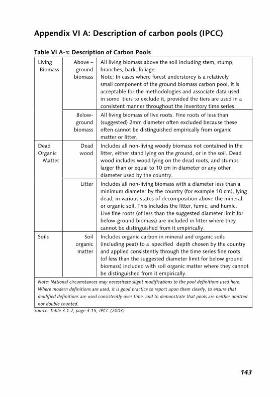
Appendix VI A: Description of carbon pools (IPCC)

Table VI A-1: Description of Carbon Pools

LivingBiomass

Above –ground

biomass

All living biomass above the soil including stem, stump, branches, bark, foliage.Note: In cases where forest understorey is a relatively small component of the ground biomass carbon pool, it is acceptable for the methodologies and associate data used in some tiers to exclude it, provided the tiers are used in a consistent manner throughout the inventory time series.

Below- ground

biomass

All living biomass of live roots. Fine roots of less than (suggested) 2mm diameter often excluded because these often cannot be distinguished empirically from organic matter or litter.

Dead Organic

Matter

Dead wood

Includes all non-living woody biomass not contained in the litter, either stand lying on the ground, or in the soil. Dead wood includes wood lying on the dead roots, and stumps larger than or equal to 10 cm in diameter or any other diameter used by the country.

Litter Includes all non-living biomass with a diameter less than a minimum diameter by the country (for example 10 cm), lying dead, in various states of decomposition above the mineral or organic soil. This includes the litter, fumic, and humic. Live fine roots (of less than the suggested diameter limit for below-ground biomass) are included in litter where they cannot be distinguished from it empirically.

Soils Soil organicmatter

Includes organic carbon in mineral and organic soils (including peat) to a specified depth chosen by the country and applied consistently through the time series fine roots (of less than the suggested diameter limit for below ground biomass) included with soil organic matter where they cannot be distinguished from it empirically.

Note:Nationalcircumstancesmaynecessitateslightmodificationstothepooldefinitionsusedhere.

Wheremoderndefinitionsareused,itisgoodpracticetoreportuponthemclearly,toensurethat

modifieddefinitionsareusedconsistentlyovertime,andtodemonstratethatpoolsareneitheromitted

nordoublecounted.Source:Table3.�.2,page3.�5,IPCC(2003)

���

Chapter VII

Examples of project specific baseline methodologies

This chapter illustrates application of baseline methodology for selected pro-jects. Baseline methodologies already approved by the CDM Executive Board (CDM-EB) are included here. The examples include the baseline methodologies for the following:

• Grid connected power generation projects

• Solid waste projects (methane recovery projects)

• Energy efficiency projects

• Industrial process improvement projects

• Fuel-switch projects

7.1 Grid Connected Power Generation ProjectsRenewable energy based grid connected power projects constitute one of the biggest project categories in terms of number of projects, submitted under the CDM. This section presents two examples of grid connected power generation projects based on:

• Biomass

• Other renewable energy resources/technologies

Though the broad contours of the two methodologies are the same, because sustainable biomass too is a renewable energy, due to certain issues associ-ated with the source of biomass, the methodology for biomass based projects is treated as a separate category. A number of methodologies for biomass-based grid connected power projects have been approved by CDM-EB since the ap-proval of methodology presented here and, therefore, a consolidated methodol-ogy on biomass based grid connected power projects is now being prepared.

���

7.1.1 Grid-connected Biomass Power Generation that Avoids Uncontrolled Burning of Biomass (AM0004)1

This methodology was developed for the A.T. Biopower Rice Husk Power Project in Pichit, Thailand. The baseline approach used in the methodology is Approach B.2

Project descriptionThis methodology was developed for a project designed to generate electricity using rice husk that would otherwise be burned in the open air or left to decay in the open. The project proposes to use the rice husk in a power plant with a net generation capacity of 20MW. The electricity generated by the plant is pro-posed to be sold to the grid through a long term contract.

Rice husk used in the project yields rice husk ash (RHA). RHA is suitable as a substitute for clinker production in cement plants. The proposed project will sell the RHA produced to an existing cement plant. The project will not claim reduc-tions from substitution of clinkers, production of which results in GHG emission, by RHA.

The project is located in a rice growing area. Of the total rice husk produced in the area, 70-75% is unused and is disposed of either in the open or burned. The project will source rice husk from more than one farm. The rice husk generation is distributed over a large area and it is difficult to collect the large quantities of rice husk needed to operate large plants.

The electricity generated by the proposed project will be sold to a grid that is dominated by fossil fuel generation sources. The total generation capacity in the grid is sufficient to meet the demand in the system. The proposed project is of a small capacity compared to the total generation capacity in the grid.

Therefore, this methodology is applicable to projects that:

• Use biomass that would otherwise be dumped or burned in an uncontrolled manner;

• Have access to an abundant supply of biomass that is unutilized and is too dispersed to be used for grid electricity generation under business as usual (BAU);

• Have a negligible impact on plans for construction of new power plants;

• Are not connected to a grid with suppressed demand;

�Alltheapprovedmethodologiescanbeaccessedfromthewebsitewithfollowingaddress:http://cdm.

unfccc.int/methodologies/PAmethodologies/approved.html.

2ApproachBis“emissionsfromatechnologythatrepresentsaneconomicallyattractivecourseof

action,takingintoaccountbarrierstoinvestment”.

���

• Have a negligible impact on the average grid emissions factor because their total generation is very small compared to the total generation in the sys-tem;

• Where the grid average carbon emission factor (CEF) is lower (and therefore more conservative as the baseline) than the CEF of the most likely operating margin candidate power generation plant.

The last applicability condition is derived based on the assessment of the base-line for a proposed project.

GHG impacts of the projectThe emissions reduction from the project activities are from two sources:

• Avoidance of methane (CH4) emissions that would have been emitted in the baseline due to the decay or burning of the biomass; and,

• Avoidance of CO2 emissions from displaced electricity, which is generated from generation sources in the grid, by electricity produced using renewable biomass.

Therefore, two baseline scenarios for the project need to be identified as the methodology combines the estimation of baseline for the two GHG impacts. These are:

• The scenario for use of rice husk in the absence of the proposed project.• The emissions from electricity generation in absence of the proposed proj-

ect.

Project boundaryThe project boundary is defined as the physical delineation of the plant site and also included off-site transportation of biomass (this could also be treated as leakage) to project site. The gases and emission sources covered in the project case and baseline are:

Projectcase• CO2, CH4 and N2O emission from biomass burning for power generation.• CH4 emission from biomass storage.• CO2, CH4 and N2O emission from transportation of biomass.• CO2, CH4 and N2O emission from auxiliary fuel consumption for power gen-

eration.

Baselinecase• CO2 emission from grid electricity generation.• CO2, CH4 and N2O emission from biomass burning in the open fields.

Baseline scenarioThere are two GHG impacts, therefore, baseline scenario has two components.

���

The applicability condition of the projects restrict the application of this meth-odology to projects where the only alternatives to the proposed use of the rice husk in the project case, given continued availability of a large surplus of rice husk, are for it either to be disposed of in the open or to be burned. The burn-ing of rice husk results in a lower GHG emission; therefore, burning of rice husk is the chosen baseline scenario.

In the absence of the proposed project, the electricity generated by the project would have been supplied by:

1. Electricity from existing generation sources last on the dispatch priority (operating margin);

2. Electricity from generation sources that would have been added to the grid in absence of the proposed project (build margin); or,

3. Electricity from both operating margin as well as build margin generation sources.

Since the methodology is applicable to projects that “have negligible impact on plans for construction of new power plants”, options (2) and (3) are rejected. Therefore, the likely baseline scenario for the second GHG impact is option (1).

Demonstration of additionality Additionality of the project is assessed as follows (Note that the methodology presented here was submitted prior to approval of the consolidated tool on ad-ditionality prescribed by CDM-EB.):

BarrierAnalysis: The project will not be implemented in the absence of CDM due to the presence of the following barriers:

(a) Investment barriers

• Return on equity is too low as compared to conventional projects;

• Real and/or perceived risk associated with the unfamiliar technology or process is too high to attract investment; and/or,

• Funding is not available for innovative projects.

(b) Technological barriers

• The project represents one of the first applications of the technology in the country, leading to technological concerns even when the technology is proven in other countries; and/or

• Skilled and/or properly trained labor to operate and maintain the technol-ogy is not available, leading to equipment disrepair and malfunctioning.

���

(c) Barriers due to prevailing practice

• There is a lack of will to change the current biomass disposal practice with or without regulations; and/or

• Developers lack familiarity with state-of-the-art technologies and are reluc-tant to use them.

(d) Other barriers

• Management lacks experience using state-of-the-art technologies, so such projects require too much management time and receive low priority by management;

• The local community may fail to see the environmental benefits of biomass power generation and so may oppose the project; and/or

• Experience and/or procedures for collecting the biomass from dispersed sources may be lacking.

A proposed project using this methodology will have to demonstrate that all or most of the above barriers are applicable to it.

Determination of the baselineThe baseline estimates the emissions from open air burning of the biomass and generation of electricity by existing generation sources in the grid, which is the baseline scenario. The baseline emissions (BL_GHGy ) are then calculated as:

BL_GHGy = BB_CH4y + EG_CO2y (1)

where,

BL_GHGy = Baseline emissions in year y

BB_CH4yCH4 = emissions in year y due to open air burning of the biomass used for electricity generation

EG_CO2yCO2 = emission in year y due to generation of the electricity by other sources.

These values are calculated as follows:

BB_CH4y = BFy x BCF x CH4F x CH4/C x GWP_CH4 (2)

where,

Bfy = biomass used as fuel during the year y measured in metric tonnes,

���

CH4F = fraction of the carbon released as CH4 in open air burning, and

BCF = carbon fraction of the biomass fuel measured as tonnes of carbon per tonne of biomass

CH4/C = mass conversion measured in tonnes of CH4 per tonne of carbon (16/12)

EG_CO2y = EGy x CEFy (3)

where,

EGy = electricity supplied to the grid by the project activity in year y, measured in megawatt hours (MWh), and

CEFy = CO2 emission factor for the electricity grid in year y, measured in tCO2e/MWh.

The CEFy is the lower of the two, viz., (i) average CO2 emission factor for all generation sources in the grid, or (ii) the ex-post calculation of operating margin CO2 emission factor for the year for which GHG emission reduction is estimated.

If a proposed project activity is located in a country/region with suppressed demand, the project participants may use a CO2 emission factor based on the “build margin”. For simplification and estimating conservative baseline, N2O emission from open air burning of surplus biomass is not considered.

Estimation of emissions reductionsThe proposed project activity generates CH4 emissions due to combustion of the biomass as well as CO2, CH4 and N2O emissions due to transportation of the biomass to the electricity generation facility. Thus, the emission reduction by the project activity during a given year is:

ERy = BL_GHGy – BBEG_CH4y – BT_GHGy – OT_GHGy – FF_GHGy (4)

where,

ERy = emission reduction by the project activity in year y,

BL_GHGy = baseline GHG emissions in year y,

BBEG_CH4yCH4 = emissions in year y due to combustion of the biomass to generate electricity,

��0

BT_GHGy = CO2, CH4 and N2O emissions in year y due to transport of the biomass to the generation facility,

OT_GHGy = CO2, CH4 and N2O emissions in year y due to on-site transport of the biomass, and

FF_GHGy = CO2, CH4 and N2O emissions in year due to fossil fuel used by the generation facility for start-up and as auxiliary fuel

The calculation of each of these values is described below.

BBEG_CH4y = BFy x BF_HV x EF_CH4 x GWP_CH4 (5)

where,

BFy = biomass used as fuel in year y, measured in metric tonnes

BF_HV = heat value of the biomass fuel used measured in TJ per tonne of biomass

EF_CH4 = CH4 emission factor for the biomass fuel measured in tonnes CH4 per TJ

GWP_CH4 = approved Global Warming Potential value for CH4 (21)

BT_GHGy = BFy/TC x AVDy x [VEF_CO2 + VEF_CH4 x GWP_CH4 + VEF_N2O x GWP_N2O] (6)

where,

BFy = biomass used as fuel during the year measured in metric tonnes

TC = truck capacity measured in tonnes of biomass

AVDy = average return trip distance between the biomass fuel supply sites and the electricity generating unit site in kilometers (km),

VEF_CO2 = CO2 emission factor for the trucks measured in tCO2/km,

VEF_CH4 = CH4 emission factor for the trucks measured in tCH4/km,

VEF_N2O = N2O emission factor for the trucks measured in tN2O/km, and

GWP_N2O = approved Global Warming Potential value for N2O (310)

���

OT_GHGy = OFy x [VEF_CO2 + VEF_CH4 x GWP_CH4 + VEF_N2O x GWP_N2O] (7)

where,

OFy = transportation fuel used on-site in year y, measured in kilograms,

VEF_CO2 = CO2 emission factor for the transportation fuel measured in gCO2/kg,

VEF_CH4 = CH4 emission factor for the transportation fuel measured in gCH4/kg, and

VEF_N2O = N2O emission factor for the transportation fuel measured in

gN2O/kg.

FF_GHGy = FFy x [GEF_CO2 + GEF_CH4 x GWP_CH4 + GEF_N2O x GWP_N2O] (8)

where,

FFy = fossil fuel used by the electricity generation unit as start-up and auxiliary fuel in year y measured in TJ,

GEF_CO2 = CO2 emission factor for the generating unit measured in tCO2/TJ GEF_

GEF_CH4 = CH4 emission factor for the generating unit measured in tCH4/TJ, and

GEF_N2O = N2O emission factor for the generating unit measured in tN2O/TJ.

LeakageThe main source of potential leakage is from diversion of biomass used by other users to the proposed project, and this results in use of fossil fuel by these other users. This leakage for the project is assumed to be zero if the proposed project activity demonstrates that:

• The proposed project will not deplete the supply of the biomass in question to the extent that it will affect the construction of other planned biomass power plants;

• Use of biomass by the proposed project does not cause competition for supply of the biomass that results in a decrease in the load factor of other existing biomass-fuelled plants; and,

• The proposed project will not deplete the supply of biomass to current users.

���

To ensure that there is an abundance of surplus biomass, the proposed project activity should demonstrate that:

• The surplus supply of biomass, for which there is no use, is more than dou-ble the biomass required to fuel all the biomass based grid-connected elec-tricity generating plants (including the proposed plant) using same biomass;

• The surplus biomass is estimated as the difference of the total biomass and the biomass consumed for conventional purposes (i.e., other than for grid electricity generation).

The proposed project should monitor the supply of biomass to ensure that an abundant surplus of biomass is maintained for the duration of the crediting period. This has been added to the methodology to address the uncertainty in the methodology from the assumption made that biomass will be available in abundance during the crediting period.

7.1.2 Consolidated Baseline Methodology for Grid-connected Electricity Generation from Renewable Sources (ACM00023)

ProjectThe project produces electricity to be supplied to the grid using renewable source of energy. The renewable source of energy used could be:

• Hydro (electricity capacity additions from run-of-river hydro power plants or hydro power projects with existing reservoirs where the volume of the reservoir is not increased) wind sources, geothermal sources, solar sources, and wave and tidal sources. Note that projects based on biomass are not covered by this methodology.

• Landfill gas, where the baseline methodology used for GHG reductions due to avoidance of release of landfill gas into the atmosphere is “Consolidated baseline methodology for landfill gas project activities (ACM0001)”.4

Projects that involve switching from fossil fuels to renewable energy at the site of the project activity are not eligible for use of this methodology.

It should be possible to clearly identify geographical and system boundaries of the grid to which the project supplies. Also, information on the characteristic of the grid is available.

3ACM:ApprovedConsolidatedMethodology

4ACM000�isdiscussedinSection7.2.

���

GHG ImpactThe implementation of this project will result in displacement or avoidance of electricity generated by other generation sources in the grid system, either exist-ing or to be added in the near future. The resultant change in GHG emission is the main GHG impact of the project activities.

Defining Project BoundaryThe spatial extent of the project boundary includes the project site and all po-wer plants connected physically to the grid to which the proposed CDM project is connected.

A spatial extent of the grid is defined by the spatial extent of the power plants that can be dispatched without significant transmission constraints. The grid may include electricity grid of more than a nation if such grids are intercon-nected. Project participants should justify their assumptions for choice of grid.

The spatial extent of the grid for assessing emissions reduction from likely addi-tions of generation source in the baseline can be expanded to include recent or likely future additions to transmission capacity that enables significant increases in imported electricity. In such cases, the transmission capacity may be consi-dered a new generation source. Emission factor for net electricity imports from existing generation sources from a connected electricity system within the same host country is determined using one of the following options:

(a) 0 tCO2/MWh,

(b) the emission factor(s) of the specific power plant(s) from which electricity is imported, if and only if the specific plants are clearly known,

(c) the average emission rate of the exporting grid, if and only if net imports do not exceed 20% of total generation in the proposed project grid, or

(d) the emission factor of the exporting grid, determined as described in steps 1, 2 and 3 (described in Section “Determination of Baseline”) below, if net imports exceed 20% of the total generation in the project electricity system.

The emission factor for imports from connected electricity system located in an-other country is assumed as 0 tons CO2 per MWh. Electricity exports should not be subtracted from electricity generation data used for calculating and monitor-ing the baseline emission rate.

AdditionalityThe additionality assessment should be done using consolidated tools for dem-onstration of additionality approved by the CDM EB. This has been explained in details in Chapter 3.

���

Determination of the baseline scenarioThe baseline scenario is electricity, in absence of the proposed project activity, would have been generated by the operation of existing grid-connected power plants and by the addition of new generation sources. The group of existing grid-connected power plants that are displaced by the project is termed as op-erating margin (OM). The group of new generation sources likely to be added is defined as build margin (BM).

Determination of the baselineBaseline is estimated as product of baseline emission factor and net power ex-ported to the grid by the proposed project.

A baseline emission factor is calculated as a combined margin (CM), that is weighted average of operating margin (OM) and build margin (BM) emission factors.

Data used for calculations of combined margin must be from an official source (where available) and made publicly available.

In case local values of net calorific value (NCV) and emission factor for fuel (EFCO2) are available, they should be used. In absence of local values, country-specific values (see IPCC Good Practice Guidance) should be used. IPCC world-wide default values should be used only if the IPCC country specific values are not available. This is applicable to all the methods.

The CM is calculated according to the following three steps.

STEP 1: Calculate the Operating Margin emission factor(s) based on any one of the following methods: (a) Simple OM (SOM) or (b) Simple adjusted OM (SAOM) or (c) Dispatch Data Analysis OM (DOM) or (d) Average OM (AOM).

Dispatch data analysis should be the first methodological choice. If this option is not selected by the project participants, they should justify why the methodol-ogy was not used.

The SOM method can only be used where low-cost/must run (LCMR)5 genera-tion sources constitute less than 50% of total grid generation, which is estimat-ed as either average generation of five most recent years or long-term normals for hydroelectricity production. Else, SAOM method should be used.

The AOM method can only be used where LCMR generation sources consti-tute more than 50% of total grid generation and detailed data to apply SAOM method and DOM method is not available.

5 Low operating cost and must run resources typically include hydro, geothermal, wind, low-cost biomass, nuclear and

solar generation. If coal is obviously used as must-run, it should also be included in this list.

���

The Simple OM emission factor (EFOM, Simple, y) is calculated as the generation-weighted average emissions per electricity unit (tCO2/MWh) of all generating sources serving the system. The LCMR power plants should be excluded from the group of generation sources used to estimate SOM. The underlying as-sumption for exclusion is that these sources are priority dispatch and, therefore, generation from these sources will not be affected by the project activities.

EF

F xCOEF

GENOM Simple y

i j y i ji j

j yj

, ,

, , ,,

,

=∑

∑ (1)

where,

Fi,j,y = amount of fuel i consumed by power sources j in year y (j refers to the power sources, other than LCMR power plants, delivering electricity to the grid. Imports to the grid should be considered as an generation source and included in group j)

COEF i,j = CO2 emission coefficient of fuel i

GENj,y = electricity (MWh) delivered to the grid by source j

The CO2 emission coefficient COEFi is obtained as

COEF NCV EF OXIDi i CO i i= × ×2, (2)

where,

NCVi = the net calorific value (energy content) per unit mass or volume of fuel i

OXIDi = the oxidation factor of fuel i

EF CO2,i = CO2 emission factor per unit of energy of fuel i

The SOM emission factor can be calculated using a 3-year average. Most recent data available at the time of PDD submission should be used to estimate the emission factor. Data for the year in which project generation occurs should be used if the SOM emission factor is updated based on ex-post monitoring.

Simple Adjusted OM emission factor (EFOM, simple, adjusted, y) is a variation of the SOM emission factor, where the electricity generation sources (including im-ports) are separated in two categories, that is, LCMR generation sources (k) and other generation sources (j):

���

EF x

F xCOEF

OM Simple Adjusted y y

i j y i

, , ,

, , ,

( )= −1 λjj

i j

j yj

y

i k y i ki k

k yk

GENx

F xCOEF

GEN,

,

, , ,,

,

∑

∑∑

+ λ∑∑ (3)

Where Fi,k,y, COEFi,k and GENk are analogous to the variables Fi,j,y, COEFj,k and GENj, described for the simple OM method earlier in equation (1). The year(s) y can reflect either of the two vintages noted for SOM above, and λ is the ratio of the number of hours for which low cost must run facilities are on the margin in a year (x, see Figure 7.1) to total number of hours in that year (8760). λy should be calculated as follows (read with Figure 7.1):

1. Plot a load duration curve (LDC) based on the chronological load data.

2. Collect data and calculate total annual generation (in MWh) from LCMR sources (i.e. ∑kGEN k,y). For example, if there are three LCMR sources in the system, total generation is GENG1+ GENG2 + GENG3.

3. Plot a horizontal line across LDC such that the area under the curve (MW times hours) equals the total generation (in MWh) from LCMR sources (i.e., ∑kGEN k,y). If there are three LCMR generation sources, then the area under the LDC should be so filled that shaded area in Figure 7.1 represents GENG1+ GENG2 + GENG3.

4. Determine the number of hours per year for which LCMR generation sourc-es are on the margin. Project the point of intersection of the horizontal line drawn in step 3 and LDC to the duration axis. Say the point of interaction is at duration y. Estimate Lambda (λ) by dividing the (8760-y = x) by 8760. λ gives the fraction of total hours in a year when LCMR generation sources are on the margin. If the horizontal line drawn in step 3 does not intersect LDC, then the LCMR sources are not on the margin and λ = 0.

Figure 7.1: Graphical depiction of steps to estimate λ.

= x/8760

y hours

Hours

MW

LDC

Intersection

87600

x hours

���

The Dispatch Data OM emission factor (EFOM, Dispatch, y) is calculated as follows:

EFE

EGOM Dispatch y

OM y

y, ,

,= (4)

where,

EGy = generation of the project (in MWh) in year y

EOM,y = emissions (tCO2) associated with the operating margin calculated as

EF EG xEFOM y h

hDD h, ,

= ∑ (5)

where,

EGh = generation of the project (in MWh) in each hour h

EFDD,h = hourly generation-weighted average emissions per electricity unit (tCO2/MWh) of the power plants (n) in the top 10% of grid system dispatch order during hour h

EF

F xCOEF

GENDD h

i n hi n

i n

n hn

,

, ,,

,

,

=∑

∑

(6)

where F, COEF and GEN are analogous to the variables described for the SOM method above (equation (1)). Index ‘n’ refers to the set of plants falling within the top 10% of the system dispatch for the hour ‘h’. The set of plants (n) is de-termined using information on: (a) the grid system dispatch order of operation for each power plant of the system; and, (b) the amount of power (MWh) that is dispatched from all plants in the system during each hour that the project activ-ity is operating (GENh). The data should be obtained from a national dispatch center. At each hour h, each plant’s generation (GENh) is stacked using the merit order, with the least merit plant at the top and highest merit plant at the bottom. The set of plants (n) consists of those plants at the top of the dispatch stack (i.e., having the least merit and, therefore, the last to be dispatched), whose combined generation (∑GENh) comprises 10% of total generation from all plants during that hour ‘h’ (including imports to the extent they are dispatched).

���

The average Operating Margin (OM) emission factor (EFOM, average, y) is calculat-ed as the average emission rate of all power plants, using equation (1) for SOM above, but including LCMR generation sources as well.

The AOM emission factor can be calculated using a 3-year average. The data used should be the most recent data available at the time of PDD submission. Data for the year in which project generation occurs should be used if the AOM emission factor is updated based on ex-post monitoring.

STEP 2: Calculate the Build Margin emission factor (EFBM,y) as the generation-weighted average emission factor (tCO2/MWh) of a sample of power plants (m), as follows:

EF

F xCOEF

GENBM y

i m yi m

i m

m ym

,

, ,,

,

,

=∑

∑

(7)

where Fi,m,y, COEFi,m and GENm,y are analogous to the variables described for the SOM method (equation (1) above) for plants m. Project participants can choose between one of the following two options to estimate the emission factor:

Option 1: Calculate EFBM,y ex-ante using the most recent information available on plants included in sample group ‘m’ at the time of PDD submission. The sample group ‘m’ consists of either:

(i) the five most recently built power plants, or

(ii) the most recently build power plants in the electricity system that comprise 20% of the total system generation (in MWh).

Project participants should use from these two options sample group that com-prises the larger annual generation.

Option 2: Calculate EFBM,y ex-post. For the first crediting period, EFBM,y must be annually updated using data for the year in which actual project generation and associated emissions reductions occur. For subsequent crediting periods, EFBM,y should be calculated ex-ante, as described in option 1 above. The sample group m should be selected like in the option 1 above. Note that power plant capac-ity additions registered as CDM project activities should be excluded from the sample group m.

���

STEP 3: Calculate the baseline emission factor EFy as the weighted average of the Operating Margin emission factor (EFOM,y) and the Build Margin emission factor (EFBM,y):

EF w xEF w xEFy OM OM y BM BM y

= +, ,

(8)

where, the weights wOM and wBM, by default, are 50% (i.e., wOM = wBM = 0.5), and EFOM,y and EF BM,y are calculated as described in Steps 1 and 2 above. Alter-native weights can be used, as long as wOM + wBM = 1, and appropriate evidence justifying the alternative weights is presented. The CDM-EB will assess the justification for alternative weights. The weighted average applied by project participants should be fixed for a crediting period and may be revised at the renewal of the crediting period.

Estimation of emissions reductionsThe project activity mainly reduces CO2 through substitution of grid electric-ity generation from fossil fuel fired power plants by renewable electricity. The emissions reduction (ERy) by the project activity during a given year y is the difference between baseline emissions, project emissions and emissions due to leakage, as follows:

ER BE PE Ly y y y= − − (9)

where,

BEy = the baseline emissions (tCO2)

PEy = the project emissions (tCO2)

Ly = leakage (tCO2)

The baseline emissions are estimated as the product of the baseline emissions factor (EFy) calculated in Step 3 and the electricity supplied by the project activ-ity to the grid (EGy in MWh).

BE EG xEFy y y

= (10)

For most renewable energy project activities, PEy = 0. However, for geothermal project activities, PEy could be non-zero. Projects emissions of geothermal proj-ect activities result from: (i) fugitive CO2 and methane emissions from release

��0

of non-condensable gases along with produced steam; and, (ii) CO2 emissions resulting from combustion of fossil fuels related to the operation of the geother-mal power plant.

Fugitive CO2 and methane due to release of non-condensable gases from the produced steam (PESy) is calculated as follows:

PES w w xGWP My Main CO Main CH CH S y

= +( ), , ,2 4 4

(11)

where, wMain,CO2 and wMain,CH4

are the average mass fractions of CO2 and methane in the produced steam, GWPCH4

is the global warming potential of methane and MS,y is the quantity of steam produced during the year y.

CO2 emissions from fossil fuel combustion (PEFFy) by the project are calculated as follows:

PEFF F xCOEFy i y

ii

= ∑ ,

(12)

where,

Fi,y = fuel consumption of fuel type i during the year y, and

COEFi = CO2 emission factor coefficient of the fuel type i.

Thus, for geothermal project activities, project emission (PEy) is calculated as follows:

PE PES PEEFy y y= + (13)

Estimation of leakageThe main emissions potentially giving rise to leakage in the context of electric sector projects are emissions arising due to activities such as power plant con-struction, fuel handling (extraction, processing, and transport), and land inunda-tion (for hydroelectric projects). Project participants do not need to consider these emission sources as leakage in applying this methodology. Project activi-ties using this baseline methodology shall not claim any credit for the project on account of reducing these emissions below the level of the baseline scenario.

���

�.� Solid Waste Projects: Consolidated Methodology for Landfill Gas Project Activities (ACM000�)After renewable energy based grid connected power projects, solid waste man-agement projects are the largest group of CDM projects submitted to CDM-EB. Such projects have twin benefits, viz., GHG reduction due to capture of meth-ane and GHG reduction from displacement of energy source by use of captured methane as energy source. The CDM-EB developed a consolidated methodol-ogy for such projects based on methodologies submitted for a number of such projects. This section presents the consolidated methodology developed by CDM-EB.

Project The proposed CDM project will install and operate gas collection system at an existing landfill site. The project activities could include:

a) Flaring of the collected landfill gas (LFG), or

b) The collected LFG is used to produce energy (e.g. electricity/thermal energy)

This project is implemented in a situation where the most likely scenario, in absence of the proposed project, is release of LFG either partially or completely into the atmosphere from landfill sites where solid waste is disposed.

This methodology does not cover solid waste projects that use a technology to either avoid generation of methane6 (such as aerobic composting of waste) or process solid waste to extract the methane prior to its disposal in landfill sites.

GHG impactThe GHG impact for projects that only collect and flare the LFG is (Category (a) in above Section) “avoidance of emission of the LFG into the atmosphere”.

For projects that both collect the LFG and use it to produce energy (Category (b) in above Section), the two GHG impacts of the project activities are:

• Avoidance of emission of the LFG into the atmosphere

• Emissions reduction from displacing or avoiding energy generation from other sources

The methodology is applicable only to avoidance of emissions of LFG into the atmosphere. Therefore, the methodology approved is applicable to projects that:

�MethaneisthelargestconstituentofLFGandtheonlysourceofGHG.

���

• Collect and use the LFG to produce energy, but, no emission reductions are claimed for displacing or avoiding energy from other sources, or

• Utilize the captured LFG to produce energy (e.g., electricity/thermal en-ergy) and emission reductions are claimed for displacing or avoiding energy generation from other sources. In this case, a separate baseline methodol-ogy for electricity and/or thermal energy displaced is developed and used. Project proponents can also use an approved methodology such as the ACM0002 (as discussed in Section 7.1.2). A small scale methodology can be used if capacity of electricity generated is less than 15MW, and/or thermal energy displaced is less than 54 TJ (15GWh), small-scale methodologies can be used.

Project boundaryThe source of emission for the project activities is from use of energy to collect the LFG or transport of LFG to locations where it is consumed. The CO2 emis-sions from flaring of collected LFG is not considered as emission, as the source of the carbon in LFG is organic and is sequestered from the atmosphere in the first place.

As this methodology is only applicable to the “avoidance of LFG emissions to atmosphere”, there are no other effects of the project activity. Therefore, the project boundary is the site of the project activity where the LFG is captured and destroyed or used.

Baseline scenariosThe possible scenarios are continuation of the past practices and the proposed CDM project activity. When it is shown that the proposed project is additional, the only baseline scenario possible is continuation of the past practices. Baseline Approach A is used to establish the baseline.

AdditionalityThe additionality assessment should be done using consolidated tools for dem-onstration of additionality approved by the CDM-EB. This has been explained in detail in Chapter 3.

Establishment of the baselineThe baseline is estimated as CO2 equivalent of methane content in the net quan-tity of LFG generated. Net LFG generated is estimated as the difference between the quantity of LFG generated and LFG captured and destroyed in compliance with regulations or contractual requirements or to address safety and odor concerns.

Estimation of emissions reductionThe GHG reduction achieved by the project activity (ERy) is estimated as sum of: (i) LFG flared during project less that required by regulation; (ii) emission reduced due to displaced electricity; and, (iii) emission reduced due to displaced

���

thermal energy. For a given year “y” ERy is calculated as:

ER MD MD xGWP EG xCEF

y project y reg y CH y ele= − +( )

, , 4 cctricity y y thermal yET xCEF

, ,+

(1)

where,

MDproject, y = Methane actually destroyed/combusted during the year (tonnes of methane (tCH4))

MDreg, y7

= Methane that would have been destroyed/combusted during the year in the absence of the project activity (tonnes of methane (tCH4))

GWPCH4 = The approved GWP value for methane (21tCO2e/tCH4)

EGy = The net quantity of electricity displaced during the year (MWh)

CEFelectricity,y8

= The CO2 emissions intensity of displaced electricity (tCO2e/MWh)

ETy = The quantity of thermal energy during the year (TJ)

CEFthermal,y = The CO2 emissions intensity of the thermal energy used

(tCO2e/TJ)

Electricity (EGy) and thermal (ETy) energy emission reductions are applicable only to case where the collected LFG is used for generating electricity or used for heat applications.

In the cases where LFG is not used for generating electricity or for thermal use, project emissions should include possible CO2 emissions resulting from combus-tion of fuels within the project boundary and emissions from electricity required for the operation of the project activity. These emissions are deducted from the ERy.

In cases where regulatory or contractual requirements do not specify MDreg,y, an Adjustment Factor (AF) should be used with proper justification, taking into account the project context.

7reg=regulatoryandcontractualrequirements

8Theemissionfactorforelectricitydisplacedintheelectricitygridshouldbedeterminedbythe

methodologyusedforcalculatingemissionreductionsduetodisplacementofelectricitytothegrid.

���

MD MD xAFreg y project y, ,

= (2)

Project proponents should provide an ex-ante estimate of emissions reductions, by projecting the future GHG emissions of the landfill. In doing so, verifiable methods should be used (such as in IPCC guidelines9). MDproject,y is determined ex-post by metering the actual quantity of methane captured and destroyed once the project activity is operational.

The MDproject,y during a year is determined by monitoring the quantity of meth-ane actually flared and gas used to generate electricity and/or produce thermal energy, if applicable.

M D M D M D M Dproject y flared y electricity y th, , ,= + + eermal y, (3)

MD LFG xw xD xFEflared y flare y CH y CH y, , , ,

=4 4 (4)

MD LFG xw xDelectricity y electricity y CH y CH, , ,

=4 44 (5)

MD LFG xw xDthermal y thermal y CH y CH, , ,

=4 4 (6)

where,

MDflared, y = the quantity of methane destroyed by flaring during the year

LFGflare, y = the quantity of landfill gas flared during the year (m3)

wCH4,y = average methane fraction of the landfill gas (m3CH4 / m3LFG)

FE = the flare efficiency (the fraction of the methane destroyed)

DCH4 = methane density (tCH4 / m3CH4) = 0.0007168

MDelectricity, y = the quantity of methane destroyed for electricity generation

LFGelectricity, y = the quantity of landfill gas fed into electricity generator

MDthermal, y = the quantity of methane destroyed for thermal energy generation

LFGthermal y, = the quantity of landfill gas fed into the boiler

9�99�IPCCguidelinesforNationalGreenhouseGasInventory.

���

LeakageSince the project activity does not result in any change in activity outside the project boundary, such as collection and transportation of solid waste, there are no leakages to be considered. The only possible leakage could be if electricity generated outside the project boundary is used for collection and flaring of LFG. But the methodology incorporates such emissions as project emissions.

7.3 Industrial Process Improvement Projects: Modification of CO2 Removal Process in an Ammonia Plant (AM0018)This methodology is based on the “Energy efficiency project by modification of CO2 removal system of Ammonia Plant to reduce steam consumption”, India (NM0037-rev.). The baseline approach is Approach A (defined in Section 2.3.2, Chapter 2).

ApplicabilityThis methodology is applicable to steam optimization projects in production processes that:

1. have homogeneous and relatively constant outputs, and

2. continuously monitor steam output of the project.

Project activityThe proposed project upgrades the existing CO2 removal process in an ammonia plant with a more energy efficient process that reduces the steam consumption in the CO2 removal system. Reduction in steam consumption leads to reduced consumption of energy (Natural gas/Naphtha) used to produce steam and, hence, reduced GHG emissions.

GHG impactThe GHG impact of the proposed project activity results from reduction in en-ergy consumption for steam production.

Project boundaryThe proposed project will affect the GHG emissions in the steam consumption and the steam generators process areas. The electricity for operating the plant, where the proposed project is located, is purchased. Therefore, if there is any change in electricity consumption due to proposed project activities then the emissions from source of electricity too will be affected.

The project boundary should, therefore, cover the following:

• Steam generator

• Source of additional electricity required due to a proposed project activity

���

• Process area where the steam consumption is expected to be reduced

AdditionalityThe additionality assessment should be carried out using the “Tool for the dem-onstration and assessment of additionality”, approved by CDM-EB (discussed in Chapter 3).

Baseline scenarioThe most likely baseline scenario is continuation of production using current processes (though steam production efficiency may improve as indicated below). The analysis of all the alternative baseline scenarios, identified in Step 1 of the additionality assessment tool, indicates that this is the most likely baseline scenario. If the most likely baseline scenario is not the continuation of produc-tion using current processes and efficiencies, then this methodology can not be applied.

Determination of the baselineThe baseline is estimated as the product of fuel combustion in the boiler, based on a benchmark Specific Steam Consumption Ratio (SSCR, steam consumption per product output), and emission factor for corresponding fuel. The SSCR for the baseline scenario is based on historical data from the existing process and is defined as the baseline energy efficiency. The difference in pre-project and post-project SSCR is used to estimate the energy savings and, hence, the GHG emission reduction.

The methodology addresses also possible increases in electricity consumption as a result of the project activity (using the small-scale methodology) and captures the impact of future retrofits and their impact on steam and CO2 savings.

The baseline SSCR is determined in three steps.

Step �: Benchmarking baseline outputA representative output value (Prep) is estimated by analyzing the historical pro-duction data of the process based on normal range of production values exclud-ing extreme values from the available values of output rate.

PP

nxA

rep

i

n

=∑

1

(1)

where,

P1, P2,….Pn = Shift/ batch-wise production values for the baseline scenario

Prep = Representative production for the day

A = number of shifts/day (batches/day) for processes (shift-wise monitoring/batch-wise monitoring)

���

Step �: Benchmarking baseline steam consumptionRepresentative steam values, corresponding to the representative production or output values, are estimated from the historical data for steam consumption as follows:

SS

nxA

rep

i

n

=∑

1 (2)

where,

S1, S2,....Sn = Shift/ batch-wise steam consumption values for baseline, cor responding to P1, ….Pn

S rep = Representative steam consumption for the day, corresponding to Prep

A = number of shifts/day (batches/day) for processes (shift-wise monitoring/batch-wise monitoring)

In the following cases, batch-wise values should be used instead of daily values:

1. If the batch time is more than 24 hours.

2. If the number of batches in a day is not an integer number (e.g.2.3 batches per day).

In cases where there are systematic patterns in production, the monitoring of historical data on production and steam consumption should represent all systematic demand variation factors with regard to representative production, energy use and equipment performance. Where there is no systematic demand variation, one-month baseline data (daily average of production values and cor-responding steam consumption values) will be adequate for establishing repre-sentative production and steam consumption.

Step �: Benchmarking of Process Specific Steam Consumption Ratio (SSCR)The SSCR is determined by the ratio of representative steam consumption and production.

SSCRS

Prep

rep

= (3)

where, SSCR is Specific Steam Consumption Ratio in the baseline

���

Emissions reductionsThe post-project SSCR benchmark is also based on monitored data and is estimated in a way similar to the baseline SSCR. Emission reductions are deter-mined ex-post as product of: (i) a difference in the baseline scenario and project case benchmark SSCR; and (ii) the actual, monitored output of the project after implementation.

Snet = Pact x SSCRdiff (4)

where,

Snet = Net reduction in steam consumption per day (kg/day)

SSCRdiff = difference in SSCR of baseline and project scenarios

Pact = Actual value of output on the day.

The net daily reduction in energy due to reduction in steam consumption is estimated as:

E net = Es x Snet (5)

where,

Enet = Net reduction in steam energy consumption per day (kCal/day)

Es = Net enthalpy of steam being supplied in boiler (kCal/kg) (The value is obtained from the monitoring of steam supply)

Es= E tot – Efw (6)

where,

Etot = Total enthalpy of steam at the boiler outlet (kCal/kg)

Efw = Heat content of feed water (kCal/kg)

The daily reduction in input energy to the boiler is estimated as:

Ein = Enet/ηb (7)

���

where

Ein = Energy input in boiler

Enet = Net reduction in steam energy consumption per day (kCal/day)

ηb = Efficiency of boiler based on direct or indirect periodically monitored values

The CO2 emission reductions (Cer) in the boiler per day are estimated as:

Cer = Ein x ∑Ffuel x Hfuel (8)

where,

Cer = CO2 emission reductions in the boiler per day

Ein = Energy input in boiler

Ffuel = Carbon emission factor for fuel to be taken based on actual laboratory tests

%Hfuel = Monitored value of % of hours per day for each type of fuel. (To be monitored)

In cases where the steam optimization project requires additional electricity, additional CO2 emissions from increased electricity is estimated and subtracted from emissions reduction estimated above (Cer).

Electricity consumption is estimated either using monitored data, if available, or based on the maximum rating (Nameplate data) of the motor, heater or any other electricity consuming device. The average daily electricity consumption (Eavg) is estimated by multiplying the representative value with the number of shifts (or batches) per day.

In the case of captive generation daily input energy to the electrical energy source is estimated as follows:

Eine = Eavg/ηg (9)

where,

Eine = Daily input energy into electrical energy source

Eavg = Average daily electricity consumption

��0

ηg = Minimum efficiency of Electricity Generating System (EGS) based on historical data of EGS operation during ‘normal range’ of output (assumed constant)

CO2 emission in case of captive generation is estimated as follows:

Cer1= Eine x Fc (10)

where,

Cer1 = CO2 emissions in case of captive generation

Fc = Carbon emission factor for fuel (IPCC)

CO2 emission in case of external grid supply is estimated as follows:

Cer2 = EavgxFgrid (11)

where,

Cer2 = CO2 emissions in case of external grid supply

Eavg = Average daily electricity consumption

Fgrid = Carbon emission factor of the selected grid.

The carbon emission factor (EF) of the selected grid is estimated using the com-bined margin method, as the average of the “approximate operating margin” and the “build margin”, where:

(i) The “approximate operating margin” is the weighted average EF (in kg CO2equ/kWh) of all electricity generating sources supplying electric-ity to the system. The generation of electricity based on hydro, geo-thermal, wind, low-cost biomass, nuclear and solar generation is not considered while estimating the EF. The EF is calculated as sum of total emission from each of the fossil fuel based electricity generation units divided by the sum of their generation in that year. The total emission from each generation unit is estimated as product of total fossil fuel consumed and the carbon intensity of the fuel.

(ii) The “build margin” is the weighted average EF (in kg CO2equ/kWh) of recent capacity additions to the system. The recently added electricity

���

generation units are identified using two methods: (i) the five most re-cent installations in the system identified by ordering all the generation units in descending order of date of commissioning; or (ii) if the total generation (MWh) of five recent additions is less than 20% of the total system generation, then electricity generation units starting from the sixth unit in the list are included till the total generation by the gener-ating units included is at least 20% of total system generation.

This grid emission factor can be applied for entire crediting period.

The net CO2 emission reduction due to project is, therefore, estimated as:

Cernet= Cer –(C er1+ Cer2) (12)

where,

Cernet = net CO2 emission reductions due to the project

Cer = CO2 emission reductions in the boiler per day

Cer1 = CO2 emissions in case of captive generation

Cer2 = CO2 emissions in case of external grid supply

LeakageThe one possibility of leakage of the proposed project arises from increased use of electricity purchased from the grid. Since this has been accounted in project emissions, there is no leakage for the proposed project.

7.4 Fuel Switch Projects: Industrial Fuel Switching from Coal and Petroleum to Natural Gas (AM0008)This methodology is based on the Fuel Switching Project implemented in Grane-ros Plant located in Chile. The chosen baseline approach for the methodology is Approach A.

Project The proposed project switches the fuel used, from coal and other fossil fuels to natural gas, for generating steam and process heat at an existing industrial facil-ity. The proposed project invests in activities that facilitate fuel switching. There are no regulations in the country that restrict the use of fuel at the project site.

���

Natural gas is a costlier fuel and switching to natural gas does not provide any efficiency gains that could off-set the incremental fuel cost and project cost. Also the switch in fuel does not affect either the process or the total output of the industrial unit.

ApplicabilityThis methodology is applicable to a project activity for switching to natural gas from the industrial fuel currently used, coal and/or petroleum fuels, which would otherwise continue to be used during the crediting period in element processes10 of a facility. The methodology is applicable under the following conditions:

1. There are no local regulations/programs that restrict the use of coal/petro-leum fuels in the facility.

2. Use of coal and/or petroleum fuels in the country and sector is less expensive than natural gas.

3. There are no major efficiency improvements from fuel switching during the crediting period.

4. The project activity does not increase the capacity of final outputs and life-time of the existing facility during the crediting period (i.e.,this methodology is applicable up to the end of the lifetime of existing facility if it is shorter than the crediting period.).

5. The proposed project activity is fuel switching applied to element processes and does not result in any integrated process change. There could be pos-sible associated changes in other energy use (such as electricity for coal pro-cessing) outside the affected element processes, which is treated as leakage.

GHG ImpactThe emissions reductions from the proposed project activities are due to switch from high carbon intensity fuel to low carbon intensity fuel.

Baseline scenarioThe baseline scenario is continuation of coal and other fossil fuel use, other than natural gas, at the industrial unit. The project proponents should prove that the

�0Examplesofthe“elementprocess”are“steamgenerationbyaboiler”and“hotairgenerationbya

furnace”.Suchaprocessgeneratesasingleoutput(suchassteam)byusingonlyasinglefuelorelectricity

source(notpluralenergysources)mainly.Ineachprocess,energyefficiencyisuniquelydefinedwith

theunitof[(unitoftheoutput)/(unitofinputenergy)].Iftheinputandoutputareidenticalforplural

processes,thosecanbebundledtoone.Ingeneral,energyefficiencyisafunctionofloadfactor.Project

participantsmaysubmitthesameCDM-PDDfordifferentelementprocessesassociatedtoaprojectasthe

methodologycouldapplytoeachoftheelementprocessesandtoitsaggregation.

���

proposed project is additional and, therefore, not a baseline scenario. Since the baseline is emission from historical activity the approach chosen is Approach A.

Additionality

As stated in the applicability condition, the proposed project is implemented in a country and sector where neither natural gas is cheaper as compared to other fossil fuels nor do the regulations require use of natural gas. Therefore, the proposed project is not likely to happen in absence of CDM. Thus, additionality should assess and demonstrate that there are no local regulations/programmes constraining the use of coal/petroleum fuels. The trends in coal and natural gas consumption in the country/region and sector should be analyzed and reported to substantiate the above contentions.

The economic investment analysis using the net present value (NPV) analysis is undertaken to assess additionality. The following parameters are used in analysis and data for these should be explicitly stated.

• Investment requirements for fuel switching

• A discount rate appropriate to the country and sector

• Efficiency of each fuel using equipment, with the current fuel and with natural gas

• Current price and projected price (variable costs) of each fuel

• Difference in operating costs for each fuel (especially, handling/treat-ment costs for coal)

• Lifetime of the project, equal to the remaining lifetime of the existing equipment(s)

• Equipment replacement costs if any during the project lifetime

The project is additional if the NPV of the project activity is negative. The residual (salvage) value of the new equipment at the end of the lifetime of the project activity should be included in estimating the NPV.

Since the present additionality is based on a comparison of project investment NPV against no investment scenario only, the methodology is not applicable to situations where the existing equipment is replaced before the crediting pe-riod ends. Therefore, the crediting period for the proposed project will not be greater than the remaining lifetime of the existing equipment.

BaselineThe baseline is GHG emission from use of baseline scenario fuel, BEy(ton of CO2 equivalents (tCO2e/yr)) during a year (y), and, is expressed as:

���

BEy = ∑i Q_Fi,y x ( EF_Fi,_CO2y + FC_Fi_CH4 x GWP_CH4 + FC_Fi_N2O x GWP_N2O) (1)

where,

Q_Fi, = Quantity of fuel i used in the baseline scenario, measured in energy units (e.g., Joule).

EF_Fi = CO2 equivalent emission factor per unit of energy of fuel i (e.g., tCO2e/Joule).

FC_Fi_CH4 = IPCC default CH4 emission factor of fuel i associated with fuel combustion, (tCH4/Joule).

FC_Fi_N2O = IPCC default N2O emission factor of fuel i associated with fuel combustion, (tN2O/Joule).

GWP_CH4 = Global warming potential of CH4 set as 21 tCO2e/tCH4

GWP_N2O = Global warming potential of N2O set as 310 tCO2e/tN2O

The parameters (variable) Q_Fi,y are calculated based on the fuel consumption in the project scenario.

Project emissions Emission reduction is the baseline less the project emissions, that is, emissions from burning of natural gas under project scenario. The project emissions PEy(measured in ton of CO2 equivalents (tCO2e/yr)) during a year (y)is expressed as:

PEy = (∑i Qi_NGy )x (EF_NG + FC_NG_CH4 x GWP_CH4 + FC_NG_N2O x GWP_N2O) (2)

where,

Qi_NGy = Quantity of natural gas used in the project scenario for replac-ing fuel i used in the baseline scenario, measured in energy units (e.g., Joule).

Q_NGy = (∑i Qi_NGy ) = Total quantity of natural gas in the project scenario for replacing all fuel used in the baseline scenario.

EF_NG = IPCC default CO2 emission factor per unit of natural gas associ-ated with fuel combustion (e.g., tCO2/Joule).

FC_NG_CH4 = IPCC default CH4 emission factor of natural gas associated with fuel combustion, measured in tCH4/Joule.

FC_Fi_N2O = IPCC default N2O emission factor of natural gas associated with

fuel combustion, measured in tN2O/Joule.

���

The variables in the baseline emissions (Qn_Fi,y) and the project emissions (Qn_NGy) are linked with the constraint relation:

Qn_Fi,y x ηn_Fi = Qn_NGy x ηn_NG (3)

where n is index for element process and i the fuel in the baseline scenario.

Fuel efficiency for use of baseline scenario fuel (ηn_Fi)and natural gas (ηn_NG) are measured either as unit of output per unit of energy (e.g., ton of output/Joule) or ratio of the output energy to the input energy, or the percentage, whichever is appropriate.

ηn_Fiand ηn_NG are functions of the load factor measured ex antebefore fuel switching (for ηn_Fi) and at the early stage of each crediting period11 (for ηn_NG). This relation is measured for each operating pattern.12 This relation is linked to the total value by summing up the processes:

∑nQn_Fi,y= Q_Fi,yand ∑nQn_NGy= Q_NGy (4)

These equations ensure that the useful heat needed is common for each ele-ment process in both project and baseline scenario. These equations are used to obtain Qn_Fi,yand Q_Fi,y, which are baseline scenario parameters by using measurable project scenario parameters.

ηn_NG shall be estimated ex anteand used to provide an estimation of the emis-sion reductions which can be expected from the project activity.

Leakage

The fugitive CH4 emission from fuel production and CO2 emission from fuel transportation are categorized as leakage of the proposed project. Emissions from fuel production/transportation are counted only if the fuel is produced/ transported in a non-Annex I country.

The leakage LEyis expressed as

LEy = [ Q_NGy x FE_NG_CH4x∑i (Q_Fi,y x FE_Fi_CH4) ] x GWP_CH4

+ [∑j (Q_TFj,y x EF_TFj)x ∑ k (Q_TFk,y x EF_TFk) ] (5)

�� Themeasurementshouldberepeatedforeachprocessnwithseveralloadfactorsinordertogetthe

curveofηnwithstatisticalsignificance.

�2 Theoperatingpatternmayincludenormaloperation,start-up,shut-down,holidayoperation,etc.

duringwhichtheloadfactorcanberepresentedbyacertainfixedvalue.

���

where,

FE_NG_CH4 and FE_Fi_CH4 are the IPCC default CH4 emission factor of natu-ral gas and fuel iassociated with fugitive emissions. In case that the effect of methane leaked from pipeline cannot be neglected, it should be included in this term.

For transportation related emissions, Q_TEj,yand EF_TEjare transportation en-ergy used and its CO2 emission factor concerning the transportation mode jfor project scenario and for mode kfor baseline scenario (such as marine, railroad or truck). In case those information and data are not available due to uncertainties and diversities in the energy market, the IPCC default value can be used. Other-wise, it could be estimated qualitatively in view of a relatively small contribution to total emissions.

Emissions reductionsThe emissions reduction ERyby the project activity is expressed as:

ERy = BEy – PE y – LEy

ERy is measured intCO2e/yr. Total emission reductions shall also be calculated ex-ante, using an estimated value for ηn_NG.

7.5 Energy efficiency projects

There is no approved methodology, developed for large projects, available for energy efficiency projects. Though, indicative baseline methodologies for small scale CDM project activities are available. These have been discussed in Chapter 4 and can be a useful guide for developing baseline methodologies for energy efficiency projects. Another useful reference towards gaining a better under-standing of energy efficiency project baseline methodologies is IEA (2000).

���

Bibliography

Baumert, K., 1999. Understanding Additionality, In: J Goldemberg and W Reid (eds.), Promoting Development while Limiting Greenhouse Gas Emissions: Trends and Baselines, UnitedNations,New York, pp. 135-143.

Beggs, K., S. Parkinson, T. Jackson, P. Morthorst, P. Bailey, 1999. Overall Issues for Accounting for the Emissions Reductions of JI projects, Proceedings of the Workshop on Baseline for CDM, New Energy and Industrial Technology Development Organization (NEDO) and Global Industrial and Social Progress Research Institute (GISPRI), February 25-26, 1999, Japan.

Bosi, M. 2000. An Initial View on Methodologies for Emission Baselines: Electricity Generation Case Study,OECDandIEAInformationPaperCOM/ENV/EPOC/IEA/SLT(200�)�2,OECD, Paris.

Bosi, M. et al., 2002. Road-Testing Baselines for Greenhouse Gas Mitigation Projects in the Electric Power Sector,OECDandIEAInformationPaperCOM/ENV/EPOC/IEA/SLT(2002)�,OECD, Paris.

Bosi, M., 2001. Fast-tracking Small CDM Projects: Implications for the Electric-ity Sector, OECD and IEA Information Paper, InternationalEnergyAgency, Paris.

Bovee, V., M. Lazarus, J.W. Martens, H.J. Wijnants, S. N. M. van Rooijen, M. T. van Wees, 2001. Grid Connected Small-Scale Renewable Energy and Energy Efficiency Projects in Martens, J.W., S.N.M. Van Rooijen, V. Bovee and H.J. Wijnants (eds.), StandardizedBaselinesforSmall-ScaleCDMActivities, ECN, The Netherlands.

Brown, S., M. Calmon, and M. Delaney, 1999: Development of a Deforestation and Forest Degradation Trend Model for the Guaraquecaba Climate Action Project.Winrock International, Carbon Monitoring Program, USA, pp. 14.

Carter, L., 1997. Additionality: The USIJI Experience, WorkshoponEnvironmentalBenefitsofAIJ, 9-10 September, Paris.

Chomitz, K., 1998: BaselinesforGreenhouseGasReductions:Problems,Precedents,Solutions. Carbon Offsets Unit, Development Research Group, World Bank, USA, pp. 62.

DEA,2003.CDMProjectManual,DanishEnergyAuthority,Denmark.

Deshun, L. and P.P. Rogers, 2000. Baseline Determination for Greenhouse Gas Abatement by Clean Development Mechanism and Joint Implementation un-der the Kyoto Protocol, Ghosh, P. (ed.) ImplementationoftheKyotoProtocol:OpportunitiesandPitfallsforDevelopingCountries, Asian Development Bank, Philippines, Development, New York: UNDP

���

E7ClimateChangeWorkingGroup(E7CCWG),2003.TheE7GuidetoImplementingProjectsundertheCleanDevelopmentMechanism,E7CCWG,Europe.

Ellis, J. & M. Bosi, 2000. Options for project emission baselines, InformationPaperCOM/ENV/EPOIC/IEA/SLT(2000)8,OECD, Paris.

Ellis, J., 1999. Experience with Emission Baselines under the AIJ Pilot Phase, OECD/IEA Information Paper, OECD, Paris.

Energy Research Institute (ERI) University of Cape Town (UCT), 2002. Clean De-velopment Mechanism: A Guide for Potential Participants in South Africa, ERI/UCT, South Africa.

Ernst Basler & Partners, 1999. Swiss-Czech Cooperation Project on Conversion of Heating Centers: An Activities Implemented Jointly (AIJ) Study,Swiss Federal Office for Foreign Economic Affairs, Zurich.

Faeth, P., C. Cort, and R. Livernash, 1994: EvaluatingtheCarbonSequestrationBenefitsofForestryProjectsinDevelopingCountries,World Resource Institute, Washington, DC, USA.

FGV Editora, 2002. The Clean Development Mechanism (CDM), A Brazilian Imple-mentation Guide, Brazil.

Friedman, S., 1999. The Use of Benchmarks to Determine Emissions Additionality in the Clean Development Mechanism, ProceedingsoftheWorkshoponBaselineforCDM, New Energy and Industrial Development Organization (NEDO) and Global Industrial and Social Progress Research Institute (GISPRI), Feb. 25-26, Tokyo, Japan, pp. 157-166.

Hamwey, R. and F. Szekely, 1998. Practical Approaches in the Energy Sector, in Goldemberg, J. (ed.) IssuesandOptions:TheCleanDevelopmentMechanisms, United Nations Development Program, New York.

ICF Consulting, 2000. Liepaja Regional Solid Waste Management Project, Moni-toring and Verification Protocol, FinalProjectDocument,Washington,DC:Prototype Carbon Fund.

Interlaboratory Working Group, 1997. Scenarios of U.S. Carbon Reductions: Po-tential Impacts of Energy-Efficient and Low-Carbon Technologies by 2010 and Beyond, Oak Ridge National Laboratory and Lawrence Berkeley National Laboratory.

International Energy Agency (IEA), 2000. Emission Baselines, Estimating the Un-known, OECD, Paris.

International Energy Agency (IEA), 2000. An Initial View of Methodologies for Emission Baselines: Case Study on Energy Efficiency, IEA, Paris.

International Institute for Environment and Development (IIED), EcoSecurities and Edinburgh Centre for Carbon Management (ECCM), 2002. Laying the

���

Foundations for Clean Development: Preparing the Land Use Sector, A Quick Guide to the Clean Development Mechanism, IIED Natural Resource Issues Paper, United Kindom.

IPCC, 2000: Land Use, Land Use Change and Forestry. R.T. Watson, I.R. Noble, B. Bolin, N.H. Ravindranath, D.J. Verardo, and D.J. Dokken (eds.), A Special report of the IPCC, Cambridge University Press, Cambridge, UK, pp. 377.

IPCC, 2003: Good Practice Guidance for Land Use, Land-Use Change and Forestry. Jim Penman, Michael Gytarsky, et.al. (eds). Published by Institute for Global Environmental Strategies (IGES).

Jepma, C., 1995: TropicalDeforestation:ASocio-EconomicApproach. Earthscan, London, United Kingdom.

Lazarus, M., S. Kartha and S. Bernow, 2000. Key Issues in Benchmark Baselines for the CDM: Aggregation, Stringency, Cohorts, and Updating, Tellus Insti-tute, Boston.

Ludeke, A.K., 1990: An analysis of anthropogenic deforestation using logistic re-gression and GIS. JournalofEnvironmentalManagement,31, 247–259.

Matsuo, N., 1999. Baseline as the Critical Issue of CDM: Possible Pathway to Standardization, IGES Discussion Papers on the Design of Effective Framework of Kyoto Mechanism, Institute for Global Environmental Strategies (IGES), Japan.

Matsuo, N., 2000. Proposal for Step-by-Step Baseline Standardization for CDM—from Project Specific to Generalized Formula, Proceeding of the IGES International Workshop on the Clean Development Mechanism, 26-28 January 2000, Kanagawa, Japan.

Meyers, S, C. Marnay, K. Schumacher and J. Sathaye. 1999. Estimating Carbon Emis-sions Avoided by Electricity Generation and Efficiency Projects: A Standardized Method (MAGPWR), Lawrence Berkeley National Lab. LBL-46063.

Ministry of Housing, Spatial Development, and the Environment of the Netherlands (MHSDEN, 2001), Operational Guidelines for Baseline Studies, Validation, Monitoring and Verification of Joint Implementation Projects, A guide for Project Developers,Version 1.0 and Volume 2a: Baseline Studies, Monitoring and Reporting; Volume 2b: Baseline Studies for Specific Project Categories; Volume 2c: Standardised Baselines and Streamlined Monitoring Procedures for Selected Small-scale Clean Development Mechanism Project Activities, www.senter.nl/sites/erupt/contents.

Organisation for Economic Co-operation and Development (OECD), 2001. Framework for Baseline Guidelines,InformationPaperCOM/ENV/EPOC/IEA/SLT(200�)�,OECD,Paris.

��0

Pembina Institute for Appropriate Development (PIAD), 2003. A User’s Guide to the Clean Development Mechanism 2nd Edition, PIAD, Canada.

Prototype Carbon Fund (PCF), 2000. Implementation Note Number 3: Baseline Methodologies for PCF Projects, World Bank, Washington.

Salon, D., 2001. An Initial View on Methodologies for Emission Baselines: Case Study on Transport, OECD and IEA Information Paper, International Energy Agency, Paris, October 2001.

Shrestha R. M. and G.R. Timilsina, 2002. The Additionality Criterion for Identifying Clean Development Mechanism Projects under the Kyoto Protocol, EnergyPolicy, Vol. 30, No. 1, pp. 73-79, 2002.

Shrestha,R.M.,andR.Shrestha,2004.Economicsofcleandevelopmentmechanismspowerprojectundersalternativeapproachesforsettingbaselineemissions,EnergyPolicy,Vol32,No�2,pp.�3�3–�374.

Shrestha,R.M.andA.Abeygunawardana,2004.CO2emission reductiondue torenewable generation projects under competitive electricity market, paperpresentedat24thAnnualNorthAmericanConferenceofUSAEE/IAEE,8-�0July2004,WashingtonDC,USA.

Shukla, P. R. and M. Mondshine, 2000. Baselines and Additionality Under the Clean Development Mechanism: Issues and Options, Climate Change Center, Confederation of Indian Industry, India.

Springer, U., 2003. Can the Risks of the Kyoto Mechanisms be Reduced Through Portfolio Diversification? Evidence from the Swedish AIJ Program, Environ-mentalandResourceEconomic, Vol. 25 pp. 501-513.

UNEP RISØ Center, 2003. CDM Information and Guidebook, Denmark.

United Nations Conference on Trade and Development (UNCTAD), An Implemen-tation Guide to the Clean Development Mechanism, UNCTAD, 2003

UNFCCC, 2001. Marrakech Accord: Report of the Conference of the Parties on its Seventh Session, held at Marrakech from 29 October to 10 November 2001: Addendum, Part Two: Action Taken by the Conference of The Parties, Volume II (FCCC/CP/2001/13/Add.2)

United Nations Development Program (UNDP), 2002. Clean Development Mecha-nism (CDM), Manual, UNDP.

Violette, D., C. Mudd, M. Keneipp and S. B. Ventures, 2000. An Initial View on Methodologies for Emission Baselines: Case Study on Energy Efficiency, OECD and IEA Information Paper, International Energy Agency, Paris.

���

CDM Baseline Glossary11

Baseline

The baseline for a CDM project activity is the scenario that reasonably represents the anthropogenic emissions by sources of greenhouse gases (GHG) that would occur in the absence of the proposed project activity. A baseline shall cover emissions from all gases, sectors and source categories listed in Annex A (of the Kyoto Protocol) within the project boundary.

Baseline approach

A baseline approach is the basis for a baseline methodology. The following three approaches as identified in sub-paragraphs 48 (a) to (c) of the CDM modalities and procedures are applicable to CDM project activities:

• Existing actual or historical emissions, as applicable; or

• Emissions from a technology that represents an economically attrac-tive course of action, taking into account barriers to investment; or

• Average emissions of similar project activities undertaken in the previous five years, in similar social, economic, environmental and technological circumstances, and whose performance is among the top 20 per cent of their category.

Baseline methodology

A methodology is an application of an approach as defined in paragraph 48 of the CDM modalities and procedures, to an individual project activity, reflecting aspects such as sector and region.

Baseline - new methodology

Project participants may propose a new baseline methodology established in a transparent and conservative manner. Project participants shall submit a proposal for a new methodology to a designated operational entity by forwarding the proposed methodology in a draft project design document (CDM-PDD), including the description of the project activity and the iden-tification of the project participants.

Baseline - approved methodology

A baseline methodology approved by the Executive Board is publicly available along with relevant guidance on the UNFCCC CDM website (http://unfccc.int/cdm) or through a written request sent to cdm-info@unfccc.int or Fax: +49 228 815 1999.

��AdoptedfromtheCDMGlossaryapprovedbytheCDMExecutiveBoard(pleaseseeCDMwebpageat

http://cdm.unfccc.int/Reference/Documents)

���

Designated Operational Entity (DOE):

An entity designated by the COP/MOP, based on the recommendation by the Executive Board, as qualified to validate proposed CDM project activities as well as verify and certify reductions in anthropogenic emissions by sources of greenhouse gases (GHG).

Host party

A Party not included in Annex I to the Convention on whose territory the CDM project activity is physically located. A project activity located in several countries has several host Parties.

Leakage

Leakage is defined as the net change of anthropogenic emissions by sources of greenhouse gases (GHG) which occurs outside the project boundary, and which is measurable and attributable to the CDM project activity.

Measurable and attributable

In an operational context, the terms measurable and attributable in paragraph 51 (project boundary) of the CDM modalities and procedures should be read as “which can be measured” and “directly attributable”, respectively.

Project activity

The Kyoto Protocol and the CDM modalities and procedures use the term “project activity” as opposed to “project”. A project activity is a measure, operation or an action that aims at reducing greenhouse gases (GHG) emis-sions.

Project boundary

The project boundary shall encompass all anthropogenic emissions by sources of greenhouse gases (GHG) under the control of the project participants that are significant and reasonably attributable to the CDM project activity. It is also termed as ‘system boundary’.

Project participants

A project participant is either a Party involved or a private and/or public entity authorized by a Party to participate, under the Party’s responsibility, in CDM project activities. Project participants are Parties or private and/or public entities that take decisions on the allocation of CERs from the project activity under consideration.

���

Stakeholders

Stakeholders mean the public, including individuals, groups or communities affected, or likely to be affected, by the proposed CDM project activity or actions leading to the implementation of such an activity.

Transparent and conservative

Establishing a baseline in a transparent and conservative manner means that assumptions are made explicitly and choices are substantiated. In case of uncertainty regarding values of variables and parameters, the establish-ment of a baseline is considered conservative if the resulting projection of the baseline does not lead to an overestimation of emission reductions attributable to a CDM project activity (that is, in the case of doubt, values that generate a lower baseline projection shall be used).

���

Appendix: Tools & Models For Estimating Baseline Emissions

Here we present selected models that can be used for estimating the baseline emissions. The models presented are a few of the many models available and are presented to familiarize readers with the structure and functioning of these models. The choice is neither a reflection of superiority of these models over others nor a reflection of our recommendation.

A large number of models have been developed for energy system analysis including demand forecasts, supply forecasts and impacts of policy shifts on the overall energy systems. These models are now adopted to estimate GHG emis-sions resulting from energy supply and demand activities. This section presents some of the econometric and optimization models, such as MARKAL, ENPEP, LEAP used for analysis of baseline emissions. Most of these models are modi-fications of models used for energy systems studies and energy demand supply assessment models. In addition, some models developed for forestry sector are presented as well, e.g., COMAP. Despite having some weaknesses these models are applicable in estimating baseline emissions for various types of CDM projects. For example, while ENPEP is more appropriate for power sector CDM projects, LEAP is more appropriate for demand side or energy efficiency im-provements CDM projects. MARKAL on the other hand, could be applicable in supply side CDM projects. It should, however, be noted that while these models are appropriate in setting baselines at the sectoral and national levels, their use for estimating baselines for a particular CDM project activity (or setting project specific baseline) needs to be analyzed. This is because, depending upon the size of CDM project, GHG emissions from a CDM project activity could be negligible compared to sectoral or national level emissions, for which these models are normally used. Nevertheless, use of these models for estimating baseline for large-scale CDM projects can not be ruled out.

In the succeeding section, structure, data requirements, underlying assumptions and limitations of each of these models are discussed. The methods to calculate baseline emissions using these models are also illustrated.

���

A.1 The MARKAL Model1

A.1.1 Structure of MARKAL

MARKAL (acronym for MARKet ALlocation) is a bottom-up type energy system model developed by the Energy Technology Systems Analysis Programme (ET-SAP) of the International Energy Agency (IEA). It is a linear programming type optimization model and based on Reference Energy System (RES)�. An overview of the MARKAL modeling system is presented in Figure A.1. As MARKAL is based on RES, it is a flexible tool to represent the energy system from primary energy resources through conversion processes, to transport, distribution and end-use devices. The demand part of the model can be specified both exog-enously and endogenously as required by users. The key characteristics of the model are as follows:

• Detailed modeling of energy supply side

• Demand and supply are balanced through optimization

• Detailed representation of depletable and renewable resources is possible

• Electricity sector is modeled in detail including generation and transmission system expansion

• The model permits a comprehensive representation of the environmental system by allowing treatment of air, water and solid waste pollutants

• The model also offers detailed demand analysis with possibility of incorpo-rating energy conservation technologies.

MARKAL consists of a user-defined network that interconnects the production (e.g., mining, petroleum extraction, etc.), conversion and processing (e.g., po-wer plants, refineries, etc.), and end-use demand for energy services (e.g., boi-lers, automobiles, residential space conditioning, etc.). The demand for energy services are also classified by economic sectors (e.g., residential, manufacturing, transportation, and commercial) and by type of end-use within a sector (e.g., re-sidential air conditioning, heating, lighting, hot water, etc.). Being an RES based model, the optimization procedure used in the model finds the best combina-

� PleaseseethefollowingliteratureformoreinformationonMARKALmodel:International

ResourcesGroup(IRG),(200�),EnergyPlanningandtheDevelopmentofCarbonMitigationStrategies:

UsingtheMARKALFamilyofModels,WashingtonDC.

2 Infact,MARKALhasbeendevelopedandusedindependentlybyvariousinternational

organisationandresearchinstitutions;hencetherearedifferentversionsofMARKALmodelwithvarying

userfriendlyfeatures.Nevertheless,thefundamentalfeatureofMARKAListhatitisbasedonRESand

employoptimizationtechnique.

���

tion of energy sources, carriers, and transformation technologies and end-use services to produce the least-cost path to deliver energy from source to end-use subject to a variety of constraints.

As described in IRG (2001)3, MARKAL can be used to analyze number of dif-ferent policy and planning issues. The current applications of this model are focussed on the analysis of policies designed to reduce carbon emissions from energy and materials consumption. MARKAL can also be used to evaluate R&D programs, energy performance standards, building codes, demand-side manage-ment and renewable technology programs, and other policies designed to guide the choice of technologies. Current versions of the model can be used to model interregional and international carbon permit trading schemes. GHG mitigation options under project-based mechanisms such as CDM and JI can also be evalu-ated using MARKAL. Moreover, ancillary or additional benefits (e.g., increased standards of living and improved health due to reduction in local pollutants) resulting from these mechanisms can be quantified in an expanded MARKAL framework.

A.1.2 Data Requirement in MARKAL

Overall cost and performance characteristics (e.g., conversion efficiencies) of technology at every stage of energy flow chain (i.e., production, transformation or conversion, transmission and utilization) are required. The key data items required by the model are summarized in Table A.1.

3 InternationalResourcesGroup(IRG),(200�),EnergyPlanningandtheDevelopmentofCarbon

MitigationStrategies: UsingtheMARKALFamilyofModels,WashingtonDC.

���

Table A.1: Key Data Items Required in MARKAL ModelResource Data Technology Data Economic Data

Resource and Production

Historical data on production; resource potential by type, and constraints

Performance of production technologies (e.g., efficiency); performance of emission control technologies if exit; emission coefficients, heat values

Costs of production technologies and emission control technologies

Transportation and Transformation

Performance of energy transformation technologies (e.g., oil refineries, gas processing plants, electricity generation efficiency); performance of emission control technologies if exit;emission coefficients and fuel quality data (heat rates, heat values)

Cost of energy transformation technologies (e.g., oil refineries, gas processing plants, electricity generation efficiency); cost of emission control technologies if exit

Demand and Utilization

Performance of energy end-use technologies (e.g., furnace, boiler, refrigerator, cooking stove etc.); emission coefficients by fuel and end-use; fuel quality data

Cost of end use technologies; Macroeconomic data such as sectoral GDP and corresponding growth rates; energy prices

���

A.1.3 Limitations of MARKAL

While the approach (RES and use of optimization techniques) is an appropriate approach for modeling energy supply systems, the demand module of MAR-KAL is weak4. Very simple techniques are used for forecasting energy demands. Energy demands are linked with GDP and are assumed to grow at the same rate as GDP. Energy demand in developing countries, in general, grow at higher rates than GDP. Thus MARKAL tends to underestimate GHG emissions in developing countries. Moreover, energy demand growth rates have declined for some end uses or sectors (e.g., manufacturing) in many developed countries and, in some cases, actually uncoupled from GDP growth rates5. MARKAL may not be an ap-propriate tool to estimate baseline emissions for demand side CDM projects. It is useful to estimate baseline emissions for supply side CDM projects, but again not an appropriate tool for power sector CDM projects.

A.1.4 Baseline Emission Calculation using MARKAL

GHG emissions are calculated based on fuel consumption. Emission coefficients are derived based on fuel and the technology used for combustion of the fuel. Fugitive emissions can also be estimated in supply side (e.g., methane emission from coal mining). Figure A.1 illustrates how energy demand is derived by sector and end-uses. GHG emissions occur in each stage (i.e., supply, conversion and end-use demand) of energy flow diagram shown in Figure A.1.

4 TraditionallyMARKALisusedasenergysupplymodel,althoughithasbeenincreasinglyused

asanenergysystemmodel.

5 Greening,L.A.,andD.L.Greene(�998),“EnergyUse,TechnicalEfficiency,andtheRebound

Effect:AReviewoftheLiterature,FinalReporttotheCenterforTransportationAnalysis,”OakRidge

NationalLaboratory.

���

Figure A.1: Structure of MARKAL Model

Source:Tseng,p.(2002),AnOverviewofUSMARKAL-MACROModel,USDepartmentOfEnergy,

Washington.

A.2 The ENPEP Model

A.2.1 ENPEP Structure

ENPEP (i.e., Energy and Power Evaluation Program) is a set of 10 integrated energy, environmental, and economic analysis tools. ENPEP developers claim that it is currently in use in over 80 countries6. The ENPEP package (consisting of 10 modules) was developed for IAEA and is distributed by this organiza-tion. These modules are non-commercial modules and are available from IAEA. Being a set of computer based energy planning tools designed to provide an integrated analysis capability, ENPEP allows users to evaluate the entire energy system (supply and demand sides), perform a detailed analysis of the electric power system, and evaluate environmental implications of different energy strategies. Each module has automated linkages to other ENPEP modules as well

� PleasevisitENPEPwebsiteathttp://www.dis.anl.gov/CEEESA/ENPEPwin.htmlfordetail

information.

��0

as stand-alone capabilities. ENPEP is structured in a modular fashion with each module having a specific objective. Each module can be executed independently or in a chain depending on the objectives of the study and the data available. The ENPEP modules along with their functional definitions are presented in Table A.2.

Table A.2: List of ENPEP Modules

Modules Function

MACRO-E Analyzing the feedback between the energy sector and the economy as a whole

MAED Bottom-up module for analyzing and forecasting energy demand

LOAD Analyze and processing hourly electric loads and to generate load duration curves and other load parameters for use in other ENPEP modules

PC-VALORAGUA Determining the optimal generating strategy of mixed hydro-thermal electric power systems

WASP-IV The latest version of WASP to determine the least-cost generating system expansion path that adequately meets electricity demand, subject to user-defined constraints

GTMax The generation and transmission maximization module to study the complex marketing and system operational issues found in today’s deregulated energy markets

ICARUS The investigation of costs and reliability in utility systems module to assess the reliability and economic performance of alternative expansion patterns of electric utility generating systems

IMPACTS Analyzing and developing a first estimate of potential physical and economic damages from air pollution using a simplified approach

BALANCE A non-linear equilibrium tool for a market-based simulation approach to determine how various segments of the energy system will respond to changes in energy prices and demands

DAM A decision analysis module to analyze tradeoffs between technical, economic, and environmental concerns

���

Some of the key features of the ENPEP model are the following:

• Demand analysis: detailed evaluation of the sectoral energy demands by sector, sub-sector, fuels and useful energy. The growth of the energy demand is determined by macroeconomic variables or other user-specified parameters (e.g. elasticities, energy intensities). The package is able to carry out energy conservation and demand side management analyses;

• Resource analysis: representation of renewable and depletable resource availability and costs;

• Supply side analysis: user-defined level of detail. Detailed evaluation of the power system configurations both current and future;

• Supply/demand balance: equilibrium solution for total energy system. En-ergy policy constraints can be imposed;

• Environmental consideration: all environmental impacts can be computed under both baseline and environmental scenarios (emissions with alternative control equipment implemented). All kinds of pollution (air, water, waste) can be taken into consideration. Incremental costs of emission can also be computed.

ENPEP has been increasingly used for the estimation of GHG emissions under the baseline and policy scenarios. The Center for Energy, Economic, and Env-ironmental Systems Analysis (CEEESA), a unit of Argonne National Laboratory, USA is the key technical support institution for ENPEP development. ENPEP has been used for GHG mitigation policy analysis studies around the globe sponso-red by the U.N. Development Program (UNDP), U.S. Agency for International Development (USAID), World Bank, U.S. Department of State (USDOS), and the International Atomic Energy Agency (IAEA). CEEESA has also developed compu-ter tools to analyze GHG mitigation policies and options, joint implementation (JI), and clean development mechanism (CDM) projects. A number of countries (e.g., Bulgaria, Jordan, Kazakhstan, Romania, Slovakia, South Korea, and Urugu-ay) have used ENPEP to develop their first and second national communications to the UNFCCC.7.

A.2.2 Data Requirement in ENPEP

Requirements for data in ENPEP depend on the purpose of the study. In the case of baseline emissions estimation, mainly four modules, namely MAED, LOAD, WASP and ICARUS could be required. Requirement for these four mo-dules also depends on the scope of the studies. MAED may not be required if the electricity load forecast is exogenously specified. ICARUS could be used (not

7 PleasevisitCEESAwebsiteathttp://www.dis.anl.gov/CEEESA/ENPEPwin.htmlforadditional

information.

���

essential) for investment additionality testing. The key data items required by the model are summarized in Table A.3.

A.2.3 Limitations of ENPEP

The key limitations of ENPEP in the context of baseline or any other GHG miti-gation analysis is that ENPEP package might be too big a tool (requiring strong institutional and modeling capacity and hence expensive) to use for estimating baseline for a CDM project activity. Although it is feasible to estimate baseline emissions for a CDM project activity using only a few modules of ENPEP, namely LOAD and WASP, these modules are not useful for CDM projects outside the power sector.

Table A.3: Key Data Items Required in ENPEP for Emission Baseline Analysis Studies

Module Resource Data Technology Data Economic Data

MAED Performance of electricity utilizing technologies (e.g., capacity, efficiency, market penetration) in each economic sectors and for every end-uses.

Costs of technologies; Macroeconomic data such as sectoral GDP and corresponding growth rates; electricity price

LOAD Hourly electricity load characteristics of electricity consuming devices and processes in all sectors for each end-uses

WASP Existing and planned capac-ity of generation facilities with supply con-straints (e.g., plant availability factor)

Performance of electricity generation technologies; emission coefficients; heat rates and heat values

Cost of electricity generation technologiesand emission control technologies

ICARUS Cost of electricity generation technologiesand emission control technologies and financial data

���

A.2.4 Baseline Emission Calculation using ENPEP

ENPEP begins with a macro economic analysis, develops an energy demand forecast based on this analysis, followed by an integrated supply/demand analy-sis for the entire energy system. It evaluates the electricity system components in detail and evaluates the environmental impacts (emissions) and resource re-quirements (land, manpower, financial) of the proposed evolution of the energy and electricity systems. Estimation of emissions using ENPEP modules is illu-strated in Figure A.2. It can be used to estimate emissions from either the power sector alone or the energy sector as a whole depending upon what modules are used.

Figure A.2: Structure of ENPEP Model

MAED

LOAD

WASPIV

BALANCE

WASPIV

MACRO-E

CapacityExpansionPlan

LoadDispatching

ElectricityGeneration

FuelConsumption

Emissions

Emissions

EnergyDemand(excludingelectricity)

���

A.3 LEAP Model8

A.3.1 LEAP Structure

LEAP (the Long-range Energy Alternatives Planning system) is developed by Stockholm Environmental Institute - Boston, USA. In contrast to MARKAL and ENPEP, LEAP is not an optimization model, rather it is a scenario-based energy accounting model. Its scenarios are based on accounting of how energy is con-sumed, converted and produced in a given region or economy under a range of alternative assumptions on population, economic development, technology, pri-ce and so on. LEAP allows for analysis in technological specification and end-use detail as the user chooses. LEAP is flexible and rich in technological specification and end-use detail as required by the users. It also provides an information bank, an instrument for long-term projections of supply/demand configurations and a vehicle for identifying and evaluating policy and technology options. The key features of the LEAP model are as follows:

• Demand analysis: detailed evaluation of the sectoral energy demands by sectors, sub-sectors, end-uses and equipment. Growth of energy demand is determined by user defined relationships for fuel share intensities, structural changes, equipment ownership.

• Energy conversion: simulation of any energy conversion sector (electric gen-eration, transmission and distribution, CHP, oil refining, charcoal making, coal mining, oil extraction, ethanol production, etc.)

• Supply side analysis: detailed evaluation of supply configurations both cur-rent and future. Iterative calculation of demand/supply balance

• Environmental analysis: environmental burdens computed as uncontrolled emissions, with alternative control equipment under alternative environ-mental regulations and with incremental cost control. The package permits comprehensive treatment of air, water, solid wastes

• Technology and Environmental Database (TED) is accommodated.

LEAP developers claim that hundreds of government agencies, NGOs and acade-mic organizations worldwide use LEAP for a variety of tasks including energy forecasting, greenhouse gas mitigation analysis, integrated resource planning, production of energy master plans, and energy scenario studies. LEAP has been

8 ThediscussionhereisbasedoninformationavailablefromLEAPwebsitehttp://www.seib.

org/leapmaintainedbytheStockholmEnvironmentInstitute(SEI),Boston,particularlythedocument

entitledLong-rangeEnergyAlternativesPlanningSystem:TrainingExercisesUpdatedVersion,July2003,

downloadedonFeb�5,2004.

���

applied at many spatial levels including local rural areas, large metropolitan cities, and at the national, regional and global level9. In the context of climate change policy analysis, LEAP has been used in national climate change studies in Argentina, Ecuador, Estonia, Hungary, Indonesia, Mauritius, Senegal and Vietnam, and regional studies in the Southern African Development Community (SADC) and the Andean Group of countries.

A.3.2 Data requirements in LEAP

The key data items required in LEAP for GHG mitigation policy analyses are listed in Table A.4.

9 PleasevisitLEAPwebsitehttp://www.seib.org/leapformoreinformationontheapplicationofLEAP.

���

Table A.4: Key Data Items Required in LEAP for Emission Baseline Analysis Studies

Resource Data Technology Data Economic Data

Resource and Production

Reserve for fossil fuels, potential of renewable energy

Performance of production technologies (e.g., efficiency); performance of emission control technologies if exit; emission coefficients, heat values

Costs of production technologies and emission control technologies

Transportation and Transformation

Performance of energy transformation technologies (e.g., oil refineries, gas processing plants, electricity generation, efficiency); capacity factors; performance of emission control technologies if exit;emission coefficients and fuel quality data (heat rates, heat values)

Cost of energy transformation technologies and emission control technologies

Demand and Utilization

Performance of energy end-use technologies (e.g., furnace, boiler, refrigerator, cooking stove, etc.); market penetration rates; existing building; vehicle stocks; energy intensity, physical outputs from the industrial sectors; specific energy consumption;emission coefficients by fuel and end-use; fuel quality data

Technology costs; Income and price elasticities;Macroeconomic and demographic data such as sectoral GDP, population, household size and corresponding growth rates; energy prices

���

A.3.3 Limitations of LEAP

LEAP is basically demand side model although it has a component that deals with supply side. The supply side component is not stronger as in the case of energy supply models such as MARKAL. It can not automatically identify least-cost systems and is less appropriate where systems are complex and a least cost solution is needed. It can not automatically yield price-consistent solutions and hence, demand forecast may be inconsistent with projected supply configura-tion.

A.3.4 Baseline Emission Calculation using LEAP

LEAP estimates emissions from each stage of an energy flow network (i.e., de-mand, transformation and production) as illustrated in Figure A.3. GHG emissi-ons to be estimated are of two types: fuel consumption (or combustion) related and non-fuel related (i.e., HFC emissions from industrial process). Moreover, fugitive emissions such as methane from coal mining and landfill gas from land-fill sites can also be estimated.

Figure A.3: LEAP model structure and estimation of emissions.

Source:Heaps,C.(2002),IntegratedEnergy-EnvironmentModelingandLEAP,SEIBoston

���

A.4 Models for Estimating Carbon Sequestration from A&R Projects

A number of models have been used for estimating the carbon pool, both for baselines as well as project scenarios. These models range from simple ac-counting models where most of variables are exogenously defined to relational models where estimated relationships and some exogenous variables are used to estimate changes in carbon pools. Two most commonly used models are briefly described below. The references for the models is provided for detailed reading on the models.

The CO�FIX (CO�FIX V.�) model, is a user-friendly tool for dynamically esti-mating the carbon sequestration potential of forest management, agroforesty and afforestation projects. CO2FIX V.2 is a multi-cohort ecosystem-level model based on carbon accounting of forest stands, including forest biomass, soils and products. Carbon stored in living biomass is estimated with a forest cohort model that allows for competition, natural mortality, logging, and mortality due to logging damage. Soil carbon is modeled using five stock pools, three for litter and two for humus. The dynamics of carbon stored in wood products is simulated with a set of pools for short-, medium- and long-lived products, and includes processing efficiency, re-use of by-products, recycling, and disposal forms. The CO2FIX V.2 model estimates total carbon balance of alternative ma-nagement regimes in both even and uneven-aged forests, and thus has a wide applicability for both temperate and tropical conditions.

The CO2FIX model was developed as part of the “Carbon sequestration in afforestation and sustainable forest management” (CASFOR) project, which was funded through the European Union INCO-DC program. The CASFOR pro-ject is a multi-institutional effort being carried out by ALTERRA in the Nether-lands, the Instituto de Ecologia from the National University of Mexico in Mexico, the Centro Agronómico Tropical de Investigación y Enseñanza (CATIE) in Costa Rica, and by the European Forest Institute in Finland. The details of the model can be downloaded from the following website http://www.efi.fi/pro-jects/casfor.

The Comprehensive Mitigation Assessment process (COMAP) model was develo-ped by the Lawrence Berkeley National Laboratory (LBL), USA. The COMAP approach is mainly dependent on finding the least expensive way of providing forest products and services while minimizing the amount of carbon emitted from the land use sector. The approach consists of the following key steps:

���

(a) Identification and categorization of the mitigation options appropriate for carbon sequestration.

(b) Assessment of the current and future land area available for these mitigation options.

(c) Assessment of the current and future wood-product demand.

(d) Determination of the land area and wood production scenarios by mitiga-tion option.

(e) Estimation of the carbon sequestration per unit area for major available land classes, by mitigation option.

(f) Estimation of the unit costs and benefits.

(g) Evaluation of cost-effectiveness indicators.

(h) Development of future carbon sequestration and cost scenarios.

(i) Exploration of the policies, institutional arrangements and incentives neces-sary for the implementation of options.

(j) Estimation of the national macro-economic effects of these scenarios.

The first step in the approach is to identify and categorize the mitigation options that are suitable for implementation in a country. The next step is to determine the forest and agricultural land area that might be available to meet current and future demand, both domestic and foreign, for wood products, and for land. Demand for wood products includes that for fuel wood, industrial wood products, construction timber, etc. Potentially surplus land in the future may be used solely for carbon sequestration or other environmental purposes. On the other hand, in many countries not enough land may be available, in which case some of the wood demand may have to be met through increased wood imports or through substitute fuel sources. Alternative combinations of future land use and wood product demand patterns will lead to different scenarios of the future.

The most-likely-trend scenario is chosen as the baseline scenario, against which the others are compared. The mitigation options are then matched with the types of future wood-products that will be demanded and with the type of land that will be available. This matching requires iterating between satisfying the demand for wood products and land availability considerations. Based on this information, the potential for carbon sequestration and the costs and benefits per hectare of each mitigation option are determined. The carbon and cost and benefit information is used to establish the cost-effectiveness of each option, which yields its ranking among other options. In addition, the information, in combination with land use scenarios, is used to estimate the total and average cost of carbon sequestration or emission reduction. Assessment of the ma-cro-economic effects of each scenario on employment, balance of payments, gross domestic product and capital investment, may be carried out using formal

�00

economic models or a simple assessment methodology. For completeness of the mitigation assessment, one should identify and explore the policies, incentives and institutions necessary to implement each option, as well as the barriers that must be overcome. The details of the model and manual can be obtained from http://eetd.lbl.gov/ea/IES/iespubs/3163.pdf.

Risø National LaboratoryRoskilde Denmark

The UNEP project CD4CDM

Baseline Methodologies for CDM Projects provides a comprehensive overview of the baseline development for CDM projects. It contains the basics of the baseline; a procedure to propose new baseline methodologies; a status of all new baseline methodologies submitted to the CDM Executive Board and examples of the Methodology Panel’s recommendations on the submitted new baselines; simplified baseline methodologies for small-scale CDM projects; a step-by-step procedure for developing baselines with a demonstration of the application of this procedure in various types of CDM project activities. A separate chapter is dedicated for readers interested to know about the process of establishing baselines for afforestation and reforestation CDM projects.

This guidebook to the CDM is produced to support the UNEP project “Capacity Development for the Clean Development Mechanism” implemented by UNEP Risø Centre on Energy, Climate and Sustainable Development in Denmark. The overall objective of the project is to develop the institutional capability and human capacity for implementation of the CDM in developing countries.

The project is funded by the Netherlands Ministry of Foreign Affairs.

Baseline Methodologies For Clean Development Mechanism Projects

Base

line M

eth

od

olo

gie

s For C

lean

Deve

lop

ment M

ech

anism

Pro

jects

�0�