Food Microbiology, 1993, 10, 43-59

A non-autonomous differential equation to model bacterial growth J. Baranyi, T. A. Roberts and P. McClure*

A F R C Inst i tute o f Food Research, Reading, Laboratory, Earley Gate, Whi teknights Road, Read ing RG6 2EF, UK

Received 26 Apri l 1992

In order to describe the dynamics of growing bacterial cultures a non-autonomous differential equation is applied. The model describes the lag phase as an adjustment period and for the lag-parameter a new definition is introduced. Some mathematical aspects of the model are described and, on the basis of more than 500 growth curves, its statistical properties are compared with the Gompertz-approach commonly used in food microbiology.

Introduction

Several approaches to modelling bac- terial growth can be found in the micro- biological literature. Following the classification of Roels and Kossen (1978) we deal here with unstructured, non- segregated growth models. This means that we suppose that (1) the biomass is homogenous; (2) the mass concentration is the only dependent variable of the system; and (3) environmental parame- ters like temperature, chemicals, etc. are not involved in the model (the possi- ble dependency on them is expressed through the dependency on the mass concentration).

In food microbiology several basic sig- moid functions (logistic, Gompertz, etc.; see, for example France and Thornley 1984), as empirical models, have become widely used. A comparative study about them was published by Zwietering et al. (1990). However, with the use of more and more exact methods in microbiology, the demand for less empirical growth

*Present address: Unilever Research, Colworth Laboratory, Colworth House, Sharnbrook, Bedford MK44 1LQ, UK.

0740-0020/93/010043 + 17 $08.00/0

models is increasing (Whiting 1992). The commonly used simple growth

model of population theory is a first order ordinary differential equation where the growth rate does not depend on time directly (autonomous, non-segregated, unstructured models). As an example one can consider the model of Turner et al. (1976), which is general enough to in- clude the logistic, Gompertz, Richards, Bertalanffy etc. growth functions.

The typical representation of a bac- terial batch culture is to plot the loga- ri thm of the cell concentration against time and, in most cases, the result is a sigmoid curve. A possible empirical so- lution is to fit a basic sigmoid function, augmented with an additive term, to these data. This way was followed by many authors in recent years in food microbiology (among them Gibson et al. 1988, Buchanan and Cygnarowicz 1990, Zwietering et al. 1990). We should keep in mind that in this case these models should not be referred to as the logistic, Gompertz etc. growth models which are meant to apply to the cell concentration and not to its logarithm.

In this paper we show a new way to apply fundamental growth models

© 1993 Academic Press Limited

44 J. Baranyi et al.

generally accepted in population theory. A mathematically formalized approach is shown which assumes that a given envi- ronment determines the potential growth rate of the culture that is higher than the actual growth rate if the time is close to the inoculation. The ratio of the actual and the potential growth rate character- izes the process of adjustment of the cells to the new environment. The most impor- tant mathematical theorems on the model have been shown in Baranyi et al. (1992) and are collected in the Appendix.

Before starting an experiment to study bacterial growth in a given environment the cells are normally grown in a favourable, more or less optimal environ- ment, in the so-called subculture, to a get a sufficient amount of cells for inoculation. Denote the pre-inoculation environment (the subculture) by El and the actual (post-inoculation) environment by E2. Suppose that E1 is sig-nificantly different (in this case more favourable) from the ac- tual environment, E 2. Our aim is to create a model which describes the lag as the process of adjustment to the new environ- ment. Note that this approach already suggests a non-autonomous model, be- cause it takes a sudden external effect on the system into account.

The mathematical formalization of the above concept can be outlined as follows.

We can consider the time of inocu- lation as zero time. Suppose that if the effect of E1 is neglected (or, which is the same, E1 = E2) then some well-known auto- nomous differential equation of the form

yc = i-t(x)x (0 < t < ~; 0 < x)

describes the bacterial growth in E2, where x denotes the cell concentration, /z(x) denotes the specific growth rate. In this case the growth rate does not de- pend on time directly, only through the cell concentration. This basic assump- tion is an implication of the fifth hypoth- esis of the framework of Frederickson et

al. (1967). Multiply the right-hand side of this differential equation by a smooth function (adjustment function) having the property that it is closer and closer to 1 as the experimental time passes. This operation expresses our wish to de- scribe the gradually diminishing effect of the previous environment. The result is a non-autonomous, separable, first order ordinary differential equation. In this way the lag phase (adjustment) is formally separated from the exponential and stat ionary phase which can be re- garded as parts of the potential growth defined by the autonomous model.

It is especially important in food safety investigations to investigate the duration of the lag phase. The classical definition of the lag (Pirt 1975) assumes that the logarithm of the cell concentra- tion forms a sigmoid curve against time and the intercept of the tangent at the inflexion with the lower asymptote is considered as the turning point indicat- ing the end of the lag phase.

By means of the adjus tment function we will give a less geometrical definition for the lag. Our lag parameter, as well as the maximum specific growth rate of the new model, will be compared with other definitions of the respective parameters.

In many respects the new model is a generalization of other models already used in the literature.

Theory In most papers on unstructured, non- segregated models of population dynam- ics the start ing point is the assumption that the growth of a population in a given environment is described by the first order ordinary differential equation

ic=tz(x)x (0_<t <o% 0 < x ) (la)

with the initial value

x(O)=xo (0 <Xo < xm~) (lb)

where x is the number of individuals per

Bacterial growth model 45

unit (concentration). The quanti ty ix(x) is called the specific growth rate and for the classical growth functions it is as- sumed that

(a)/x(x) is defined for x0 < x < xm~ (x,~ is fixed)

(b) t~(Xo) > 0 and tX(Xm~) = 0 (C) /X(X) is continuously differentiable in

its domain and dlx /dx is strictly neg- ative there.

Under these conditions the so-called initial value problem defined above (differential equation together with its initial value) has a unique solution, de- noted here as fit). This solution is mono- tone increasing and converges to xm~ as t ~ ~ (Vance 1990).

Equation (la) is a so-called auto- nomous differential equation because its right-hand side depends on the un- known dependent variable itself and it does not depend on time directly. Its general solution takes the form x(t) = f(t-T), where T is a constant character- izing a shift parallel to the t axis (it can be considered as a delay in growth). The value of T can be uniquely defined by fixing an initial value for x(0).

Depending on the choice of/~(x), dif- ferent sigmoid functions can be obtained which satisfy (la). Note that the condi- tion (c) corresponds to the assumption that the larger the population density the lower is its specific growth rate. As can be shown mathematically, this means that the time-derivative of the logarithm of the wanted growth func- tion is strictly monotone decreasing.

Consider the experimental time (i.e. the time elapsed from inoculation) as the independent variable, t. Fix the time of the inoculation as t = 0. Our model will be defined for non-negative values of t in the following way.

We postulate tha t after inoculation the cell concentration of the culture is described by the initial value problem

yc = a(t)tL(x)x (0 <__ t < ~; 0 < x) (2a) x(O) = Xo (0 < xo < x.,,=) (2b)

where:

(a)/~(x) is independent of E1 and satisfies the conditions assumed under (la) and (lb).

(b) a(t) depends on E1 and E2 and 0 < a ( t ) < l ( 0 < t < ~ ) . (3)

Furthermore if a(t) ~ 1 monotone in- creasingly as t --> ~ then we say that a(t) is an adjus tment function from E1 to E2.

We say that (la), (lb) define the po- tential growth, and (2a), (2b) define the actual growth in the environment E2.

The interpretation of these defini- tions is as follows: The given, actual environment E2 and the inoculum level, Xo, uniquely determine the potential growth curve, according to which the population would be able to grow if the previous environment had been the same as the present environment (E~ = E2: no need to adjust, that is a(t) -= 1). The potential growth of the population is described by the autonomous equa- tion (la). The actual growth, however, is described by (2a) and (2b) which means that after inoculation (a sudden change in the environment from El to Ee), the cells' actual specific growth rate is heav- ily influenced by the fact that the time is close to zero. Later, however, the effect of the previous environment diminishes, until some time after the inoculation it has little or no effect and the cells grow essentially at their potential growth rate, /x(x), defined by the new environ- ment, E2. Therefore the ratio of the ac- tual and the potential growth rate, i.e. the adjustment function, is expected to increase from zero (no growth because of lagging) to 1 (total adjustment).

Theorem 1 in the Appendix gives the solution g(t) for the actual growth curve by means of the functions f and a. Its form is:

g(t) = f(A(t)), (4)

46 J. Baranyi et al.

where A(t ) is the integral function of a(t).

A class of adjustment functions of the form

t n an(t) = - - , (5)

A" + t n

where A and n are positive numbers, proved to be generally very effective when fitting our viable counts data. This adjustment function can be derived in the following way:

Suppose that the growth is controlled by a critical substrate, or product, say P, which is vital to ensure growth in the new environment and it was present in a negligibly small amount in the previ- ous environment. Furthermore suppose that the dependence of growth on this product follows the well-known Michaelis-Menten rule:

P(t) = ~ (x)x, (6)

Kp + P(t)

where Kp is the so-called saturation con- stant. This gives the adjustment func- tion the form:

P(t) a(t) = . (7)

Kp + P(t)

After rearrangement:

P(t)

go ~(t) = (8)

P(t) 1 + -

go The quanti ty P ( t ) / K s is dimensionless.

Suppose that atter inoculation the production of the critical product de- pends on E2 and is proportional to the n-th power of time:

P(t)Kp = ( t ) n (9)

Here n characterizes the rate at which P

is built up around t = A (the larger is n, the faster is the accumulation of P) where A is the time point were P = Kp. Subst i tute the lat ter expression in (7) and the adjustment function of the form (5) can be obtained.

The interpretation above explains the next definitions. We call the parameter

of the adjus tment function of the form (5) the lag parameter . In what follows we refer to an(t) as a d j u s t m e n t func t ion o f order n.

Note that Theorem 2 in the Appendix gives an estimation of what happens if the adjus tment function is derived in a different way. Roughly it can be said that if two adjus tment functions are close to each o t h e r (this 'closeness' is measured by the integral of their differ- ence), then the respective actual growth curves will also be close to each other.

Some properties of the adjustment function (5) are:

- a,(O) = 0; an(A) = 1/2 - an(t) is strictly monotone increasing - an(t) ---> 1 (t ~ ~) - if n > 1 then

a~ d a n / d t = O a t t = O b/ an(t) has an inflexion point at

n

T n = ~¢/(n - 1) / (n + 1) A. (10)

Generally it simplifies the calculation of the An(t) integral function if the next relation is used:

t fs° An(t )= An + s n 0

where,

ds = A -Bn (II)

I 1 Bn(t) = - - d s . (12)

l + s n o

Theoretically the integral function Bn(t) can be expressed by elementary functions for a fixed positive integer, n, but for larger values of n the expression

Bacterial growth model 4 7

is more and more complicated. For bac- teriological data representing a broad range of growth conditions for a variety of organisms, an adjustment function of order 4 proved to be satisfactory to char- acterize the transition from the lag to the exponential phase. In this case the expression for B4(t) is:

B4(t) = ) 1 t2 + X/2t + 1 _ _ I n _ + ~ / ( t )

2V2 t 2 - ~ / 2 t + 1 (13)

where,

arctan - -

y(t)= 7r/2

arctan

V 2 t

1 - - t ~

(t < 1)

(t = 1)

+Tr ( t > l )

(14) X/2t

1 - t 2

(See, for example, Korn and Korn 1973).

Some theoretical aspects of this ad- jus tment function are summarized in Theorems 4-5 in the Appendix. Since the adjus tment function, an(t), is the derivative of An(t), and an(t) converges to 1 as the time elapses, An(t) plays the role of delayed time; i.e. A,( t) is closer and closer to the function t-A and the ac- tual growth function is closer and closer to a delayed potential growth function, fit-A). Therefore, this delay, A, can be considered as a good approximation of the length of the lag phase in the actual growth.

Now we examine two important classes of autonomous growth as poten- tial growth.

(a) Pure exponential g r o w t h as potent ial g rowth

When collecting data from experiments, sometimes, for one reason or other, there are no data to indicate the station- ary phase of the growth curve. In these cases a computer program fitted a sig-

moid curve to the data can easily fail be- cause of the lack of information to esti- mate the parameter characterizing the stat ionary phase. Still it is desirable not to waste the results of these experi- ments. The solution can be either to fix the parameter characterizing the sta- t ionary phase or to have a growth func- tion which models only the lag and the exponential phase.

The new approach introduced in this paper is suitable to get a growth func- tion of the lat ter type. For this purpose consider the pure exponential growth as potential growth and combine it with our adjustment function given in (5). (Although in this case the condition (c) under (la) and (lb) is not satisfied, ac- cording to the Theorems in the Ap- pendix the connection between the po- tential and actual growth remains the same as above). The respective equa- tions are:

Potential growth curve (solution of ( la)-(lb)):

fit) = xoexp (l~m~t).

growth curve (solution of Actual (2a)-(2b)):

g(t) = xoexp (/~mo~A,(t)).

where A,( t) is defined by (11), (12).

In the study of batch cultures in food microbiology it is more common to con- sider the logarithm of the cell concentra- tion as the dependent variable. If this is the natural logarithm:

y(t) = In x(t),

then the slope of the tangent of the y(t) curve will be the specific growth rate. Transform the actual growth curve into the y,t plane:

y(t) =Yo + I~: ,An( t ) (15)

where Yo = In xo.

By means of the obtained model (15)

4 8 J. Baranyi et al.

we can demonstrate the role of the pa- rameters ~ and n also in the following way: (i) Second-derivat ive-concept . Recently, Buchanan and Cygnarowicz (1990) de- fined the end of the lag phase as the time point where the second derivative of the logarithm of the actual growth curve has its maximum, i.e. where the third derivative of A,( t ) is zero. Since an(t) is the first derivative of A,(t), the point in question is the inflexion point T, of the an(t) adjustment function. It can be seen from Eqn (10) tha t in our adjustment function, T, is very close to

(for example, for n = 4:T4 ~- 0-9 ~). In fact from (10) it follows that T, ~ A monotone increasingly as n ~ oo. This demonstrates again why we can call out A parameter the lag parameter . (Note tha t the classical lag definition by means of the tangent drawn to the inflexion of the growth curve could not be applied here because the growth curve itself has no inflexion?) (ii) Step-funct ion-concept . It can be checked that a,(t) --~ a~(t) as n -o ~, where a=(t) is the step function

0 (t < A) a=(t) = 1/2 (t = A) (16)

1 (t > A).

This function was implicitly used by Kono (1968) to model the lag phase. There the author used a constant factor which was 0 for t < t 1 and 1 for t > t~, where t, was a 'suitable' t ime (see also Barford et al. 1982). In our model A plays the role of t~. For a=(t) the definite integral function is A=(t), where

0 (t < ~) A=(t) = t - ,\ (t >_ ~) (17)

(Theorem 4 in the Appendix). Therefore the actual growth curve of

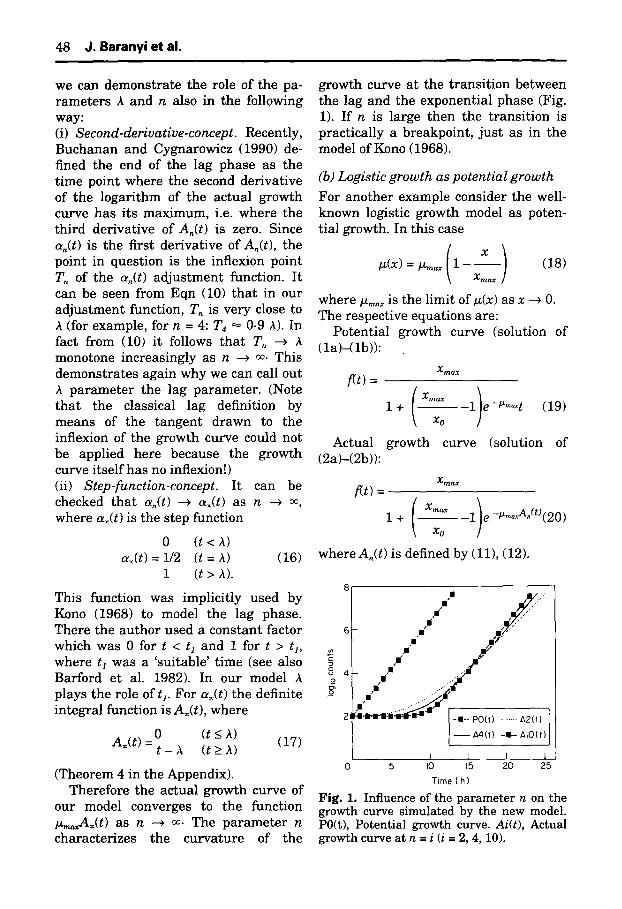
our model converges to the function /~,~A~(t) as n --* ~. The parameter n characterizes the curvature of the

growth curve at the transi t ion between the lag and the exponential phase (Fig. 1). If n is large then the transi t ion is practically a breakpoint, jus t as in the model of Kono (1968).

(b) Logis t ic g rowth as po ten t ia l g rowth

For another example consider the well- known logistic growth model as poten- tial growth. In this case (x)

/x(x) =/~m~ 1 - - (18) Xmax

where/xm~ is the limit of/z(x) as x -~ 0. The respective equations are:

Potential growth curve (solution of ( la)-( lb)) :

]~t) = Xm~

Actual (2a)-(2b)):

Xrna.x f'(t) =

1 + -

Xo

xmax ) 1 + . 1 e - t 'm ' t (19)

Xo

growth curve (solution of

1)e -~m~A,(t) ( 20 )

where A,( t ) is defined by (11), (12).

• f n" ...'"'

,J" / .."'"

• I~ | t I 'J 6

i

' ~ • mG hi" " f " "

8 4 9 - I( ..'"'"

2 : l . l . l - I : / ~ r u ~ -.ii-- PO0) ........ A2(t)

I - - r~('l - , - ~Lo(,I I

1 I I 1 I 0 5 I0 15 20 25

Time ( h )

Fig. 1. Influence of the parameter n on the growth curve simulated by the new model. P0(t), Potential growth curve. Ai(t), Actual growth curve at n = i (i = 2, 4, 10).

Bacterial growth model 49

As with (15), we transform the obtained model (20) to the y , t plane, where y(t) = In x(t).

We get:

y(t) = ym~-ln (1 + (e-'Y~-Yo-1)e-t~=An(t)),

(21a)

where y , ~ = In x,~.

As can be checked, the formula above can be writ ten in another form:

egmo~.(t))_~ y(t) =yo + P-m~An(t) + In 1 + ~ ]

g

(21b)

This other form of the same function highlights the connection with the case, when the pure exponential growth was used for potential growth (see Eqn (15)). It is well-known that i fh << 1 then

ln(1 + h) ~ h

therefore the formula (21b) shows that close to the inoculation, where the frac- tion in (21b) is small, practically there is no difference between (15) and (21a) - - that is, the maximum population does not yet influence the growth. In the Dis- cussion we return to the computational consequences of this connection.

Without going into detail, we mention the possibility of choosing the more gen- eral Richards-curve (see for example, France and Thornley 1984) as potential growth. It differs from the logistic curve in the sense that it has an extra (posi- tive) parameter, denoted by m here, which characterizes the curvature be- fore the stat ionary phase. The choice m = 1 is equivalent to the choice of the logistic curve. The formulae, respective to (21a) and (21b) can be writ ten as:

1 y(t ) = y , ~ - - ~ In (1+ (e ~"~-y°~

(22a)

y(t) = Yo + I~m~,An(t) +

l l n ( 1 +e""~A"(t)-I I m em{ymax--Yo} ]

(22b)

Results

Our concept will be demonstrated with the fourth order adjustment function as(t) combined with the logistic growth model above as potential growth curve. Choos- ing n = 4 for the order of the adjustment function has mainly computational ad- vantages. By means of the Eqns (11), (14) it is possible to substitute an explicit ex- pression for the actual growth curve in a curvefitting procedure.

We found that, generally, higher val- ues of n (usually between 6 and 10) give bet ter fit, but either fixing the curvature parameter n at an integer value larger than 4, or fitting its value to a param- eter estimating procedure, needs some computational tricks and it is advisable to adjust some well-known codes (for ex- ample Press et al. 1990) to solve these problems. These computational aspects of our approach are being summarized presently in a separate paper.

From several points of view Zwieter- ing et al. (1990) found the Gompertz curve the best from a range of growth models. Also Gibson et al. (1988) re- ported that the Gompertz function was the best fitting curve when analysing their data. This is why we chose the Gompertz function to compare it with one of our family of growth models: the logistic growth combined with fourth order adjustment function. In this case the formula for the logarithm of the cell concentration of a growing culture is given by (21) and (11).

Gibson et al. (1988) published the es- t imates of the maximum specific growth rate and the lag obtained by fitting four parameter Gompertz curves to a num- ber of S a l m o n e l l a - d a t a . For a numeric

50 J. Baranyi et al.

demons t r a t ion we selected the first 40 curves of t h a t da tase t . Our curvef i t t ing procedure was run on the same data- points.

Program 1 fi t ted four p a r a m e t e r Gomper tz curves, as sugges ted by Gib- son et ai. (1988), to the m e a s u r e d loglo counts by a s t a n d a r d leas t squares me thod us ing Marqua rd t ' s a lgor i thm wi th single precis ion a r i t hme t i c (Press e t al. 1990). The m a x i m u m specific growth ra te was calcula ted as the slope of the t a n g e n t a t the inflexion of the yl(t) curve where yl(t) is a fi t ted Gomper t z function, a u g m e n t e d by an addi t ive pa- r a m e t e r (see Gibson et al. 1988). The lag was calculated as the in te rcep t of this m a x i m u m slope wi th the lower asymp- tote of the curve. In wha t follows,/~1 and ~ will denote the va lues of these growth p a r a m e t e r s as e s t ima ted by Program 1.

Program 2 f i t ted our f o u r - p a r a m e t e r model, a logistic potent ia l growth wi th four th order a d j u s t m e n t funct ion, us ing the same Marqua rd t -me thod . The esti- ma t ed growth p a r a m e t e r s (/~m~, maxi- m u m potent ia l g rowth rate; A, lag-pa- r a m e t e r of the a d ju s tmen t function) will be denoted by p~ and A2 respect ively.

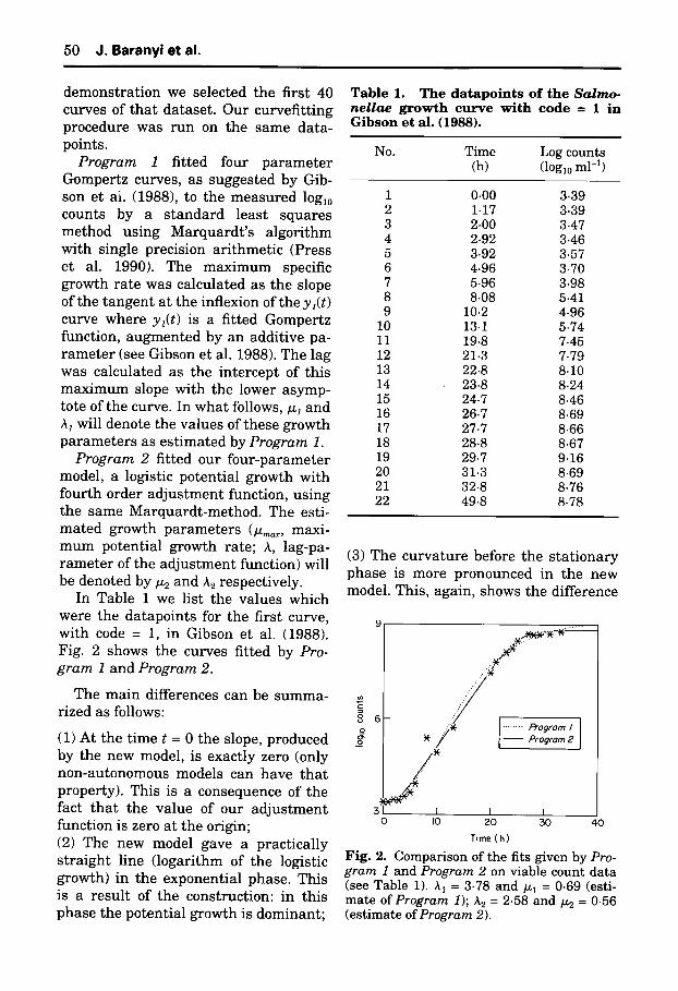
In Table 1 we list the va lues which were the da tapo in t s for the first curve, wi th code = 1, in Gibson et al. (1988). Fig. 2 shows the curves f i t ted by Pro- gram 1 and Program 2.

The ma in differences can be summa- r ized as follows:

(1) At the t ime t = 0 the slope, produced by the new model, is exact ly zero (only non-au tonomous models can have t h a t property) . This is a consequence of the fact t h a t the va lue of our a d j u s t m e n t funct ion is zero at the origin; (2) The new model gave a pract ica l ly s t r a igh t line ( logar i thm of the logistic growth) in the exponent ia l phase . This is a resu l t of the construct ion: in this phase the poten t ia l g rowth is dominan t ;

T a b l e 1. T h e d a t a p o i n t s o f t h e Salmo- nellae g r o w t h c u r v e w i t h c o d e = 1 i n G i b s o n et al . (1988).

No. Time Log counts (h) (loglo ml-b

1 0.00 3.39 2 1.17 3-39 3 2.00 3-47 4 2.92 3.46 5 3.92 3.57 6 4.96 3.70 7 5-96 3.98 8 8-08 5.41 9 10.2 4.96

10 13.1 5-74 11 19.8 7.45 12 21.3 7.79 13 22.8 8.10 14 23.8 8.24 15 24.7 8.46 16 26.7 8.69 17 27.7 8.66 18 28.8 8.67 19 29.7 9.16 20 31.3 8.69 21 32-8 8.76 22 49.8 8.78

(3) The cu rv a tu r e before the s t a t i ona ry phase is more p ronounced in the new model. This, again, shows the difference

g 8 6 o / :: ...... ~ o g r o m / / ~ Proffrom2 ]

F I I I

I0 20

Time ( h )

40

Fig. 2. Comparison of the fits given by Pro- gram 1 and Program 2 on viable count data (see Table 1). A 1 = 3.78 and/~1 = 0.69 (esti- mate of Program 1); A 2 = 2.58 and/~2 = 0.56 (estimate of Program 2).

Bacterial growth model 51

between the curvature of the logarithm of the logistic curve and the curvature of the Gompertz curve before the station- ary phase.

Before comparing Program 1 and Pro- gram 2 on a larger dataset we show an example for the use of the pure exponen- tial growth as potential growth:

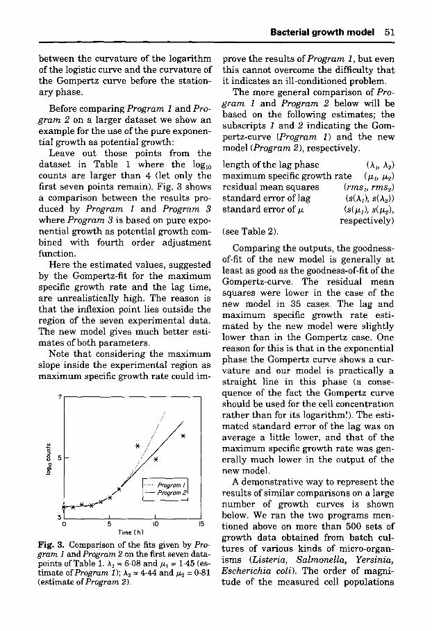
Leave out those points from the dataset in Table 1 where the loglo counts are larger than 4 (let only the first seven points remain). Fig. 3 shows a comparison between the results pro- duced by Program 1 and Program 3 where Program 3 is based on pure expo- nential growth as potential growth com- bined with fourth order adjustment function.

Here the estimated values, suggested by the Gompertz-fit for the maximum specific growth rate and the lag time, are unrealistically high. The reason is tha t the inflexion point lies outside the region of the seven experimental data. The new model gives much better esti- mates of both parameters.

Note tha t considering the maximum slope inside the experimental region as maximum specific growth rate could im-

...-" :'Y

. . . . . . . P r o g r o m

51 i I 0 5 IO 15

Time ( h )

Fig. 3. Comparison of the fits given by Pro- gram I and Program 2 on the first seven data- points of Table 1. A1 = 6.08 and/~1 = 1.45 (es- timate of Program 1); A2 = 4-44 and/12 = 0.81 (estimate of Program 2).

prove the results of Program 1, but even this cannot overcome the difficulty tha t it indicates an ill-conditioned problem.

The more general comparison of Pro- gram 1 and Program 2 below will be based on the following estimates; the subscripts 1 and 2 indicating the Gom- pertz-curve (Program 1) and the new model (Program 2), respectively.

length of the lag phase (AI, A2) maximum specific growth rate (/~1,/~2) residual mean squares s tandard error of lag s tandard error of/~

(see Table 2).

(rms l, rms2) (s(A~), s(A2)) (s(t~1), s(~),

respectively)

Comparing the outputs, the goodness- of-fit of the new model is generally at least as good as the goodness-of-fit of the Gompertz-curve. The residual mean squares were lower in the case of the new model in 35 cases. The lag and maximum specific growth rate esti- mated by the new model were slightly lower than in the Gompertz case. One reason for this is tha t in the exponential phase the Gompertz curve shows a cur- vature and our model is practically a straight line in this phase (a conse- quence of the fact the Gompertz curve should be used for the cell concentration rather than for its logarithm!). The esti- mated s tandard error of the lag was on average a little lower, and tha t of the maximum specific growth rate was gen- erally much lower in the output of the new model.

A demonstrative way to represent the results of similar comparisons on a large number of growth curves is shown below. We ran the two programs men- tioned above on more than 500 sets of growth data obtained from batch cul- tures of various kinds of micro-organ- isms (Listeria, Salmonella, Yersinia, Escherichia coli). The order of magni- tude of the measured cell populations

52 J. Baranyi et al.

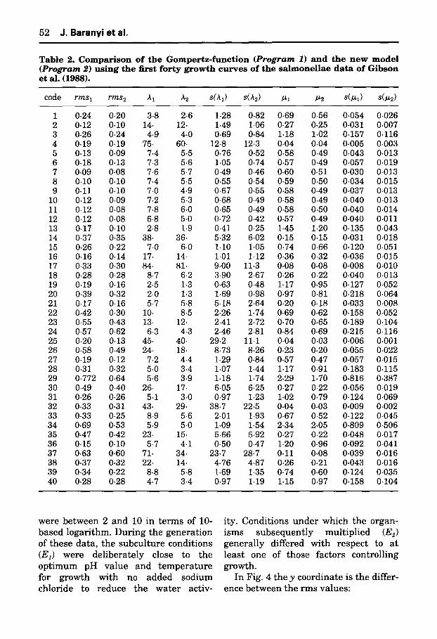
Table 2. C o m p a r i s o n o f the G o m p e r t z - f u n c t i o n ( P r o g r a m 1) a n d the n e w m o d e l ( P r o g r a m 2 ) u s i n g the first for ty g r o w t h c u r v e s o f the s ~ l m o n e H a e data o f G i b s o n et al. (1988).

code r m s 1 r m s 2 ~t 1 ~2 s(/tl) s(~2) ~tl P~2 s(~l) s(p~2)

1 0.24 0.20 3.8 2.6 1.28 0.82 0.69 0.56 0.054 0.026 2 0.12 0.10 14. 12. 1.49 1.06 0.27 0.25 0.031 0.007 3 0.26 0.24 4-9 4.0 0.69 0.84 1.18 1.02 0.157 0.116 4 0.19 0-19 75. 60. 12.8 12.3 0.04 0.04 0.005 0.003 5 0.13 0.09 7.4 5.5 0.76 0.52 0.58 0.49 0.043 0.013 6 0.18 0.13 7-3 5-6 1.05 0.74 0.57 0.49 0.057 0.019 7 0.09 0.08 7.6 5.7 0.49 0-46 0.60 0.51 0.030 0.013 8 0.10 0.10 7.4 5.5 0.55 0.54 0.59 0.50 0.034 0.015 9 0.11 0.10 7.0 4.9 0.67 0.55 0.58 0.49 0.037 0.013

10 0.12 0.09 7.2 5-3 0.68 0.49 0.58 0.49 0-040 0-013 11 0.12 0.08 7.8 6.0 0.65 0.49 0.58 0.50 0.040 0.014 12 0.12 0.08 6.8 5.0 0.72 0.42 0.57 0.49 0.040 0.011 13 0.17 0-10 2.8 1.9 0.41 0-25 1.45 1.20 0-135 0.043 14 0.37 0.35 38. 36- 5.32 6.02 0-15 0.15 0.031 0-018 15 0.26 0.22 7.0 6.0 1.10 1.05 0.74 0.66 0.120 0.051 16 0.16 0.14 17. 14. 1.01 1.12 0.36 0.32 0.036 0.015 17 0.33 0.30 84. 81. 9.00 11.3 0.08 0.08 0.008 0.010 18 0.28 0.28 8.7 6.2 3.90 2-67 0.26 0.22 0.040 0.013 19 0.19 0.16 2.5 1.3 0.63 0.48 1.17 0.95 0-127 0.052 20 0.39 0.32 2.0 1.3 1.69 0.98 0-97 0.81 0.218 0.064 21 0.17 0-16 5.7 5.8 5-18 2.64 0.20 0.18 0.033 0.008 22 0.42 0.30 10. 8.5 2.26 1.74 0.69 0.62 0.158 0.052 23 0.55 0.43 13. 12. 2.41 2.72 0.70 0.65 0.189 0.104 24 0.57 0.62 6.3 4.3 2.46 2.81 0.84 0.69 0.215 0.116 25 0.20 0.13 45. 40- 29.2 11.1 0-04 0.03 0-006 0.001 26 0.58 0.49 24. 18. 8.73 8.26 0.23 0.20 0.055 0.022 27 0.19 0.12 7.2 4.4 1.29 0.84 0.57 0.47 0.057 0.015 28 0-31 0.32 5-0 3.4 1.07 1.44 1.17 0.91 0.183 0.115 29 0.772 0-64 5.6 3.9 1.18 1-74 2.29 1.70 0.816 0.387 30 0.49 0.40 26. 17. 6.05 6.25 0.27 0.22 0.056 0.019 31 0.26 0.26 5.1 3.0 0-97 1.23 1.02 0.79 0.124 0.069 32 0.33 0.31 43. 29. 38.7 22.5 0.04 0.03 0.009 0.002 33 0.33 0-25 8.9 5.6 2.01 1.93 0.67 0.52 0.122 0.045 34 0.69 0.53 5.9 5-0 1.09 1.54 2.34 2.05 0.809 0.506 35 0.47 0.42 23. 15. 5.66 5-92 0.27 0.22 0.048 0.017 36 0.15 0-10 5-7 4.1 0-50 0.47 1.20 0.96 0-092 0.041 37 0-63 0.60 71. 34. 23.7 28.7 0.11 0.08 0.039 0.016 38 0.37 0.32 22. 14. 4.76 4-87 0.26 0.21 0.043 0.016 39 0-34 0.22 8.8 5.8 1.69 1.35 0-74 0.60 0.124 0.035 40 0.28 0.28 4.7 3.4 0.97 1.19 1.15 0.97 0.158 0.104

were b e t w e e n 2 a n d 10 in t e r m s of 10- i ty. Cond i t ions u n d e r which the o rgan- b a s e d l oga r i t hm. D u r i n g the g e n e r a t i o n i sms s u b s e q u e n t l y m u l t i p l i e d (E~) of t he se da t a , t he s u b c u l t u r e condi t ions g e n e r a l l y d i f fered wi th r e s pe c t to a t (El) were d e l i b e r a t e l y close to the l e a s t one of those fac tors con t ro l l ing o p t i m u m pH v a l u e a n d t e m p e r a t u r e growth . for g rowth wi th no a d d e d s o d i u m In Fig. 4 t he y coo rd ina t e is t he differ- ch lor ide to r educe the w a t e r act iv- ence b e t w e e n the r m s va lues :

Bacterial growth model 53

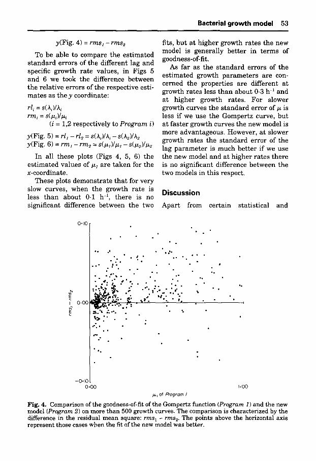
y(Fig. 4) = r m s z - r m s e

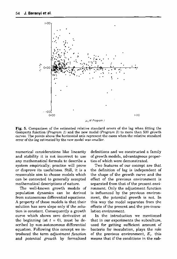
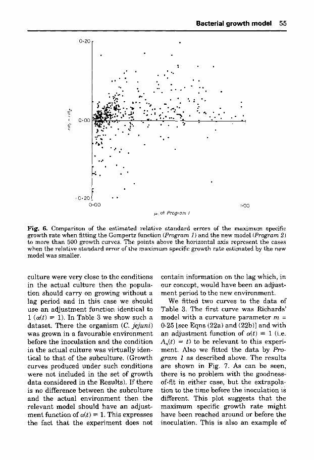
To be able to compare the e s t ima t ed s t a n d a r d e r rors of the d i f ferent lag and specific growth r a t e values , in Figs 5 and 6 we took the difference be tween the re la t ive e r rors of the respect ive esti- ma te s as the y coordinate:

r l i = S(Ai) /Ai

r m i = s ( l x i ) / l x i

(i = 1,2 respec t ive ly to P r o g r a m i )

y(Fig. 5) = r l l - r l 2 = s(Ai)/Ai - s(Ae)/A2 y(Fig. 6) = r m l - r m 2 = s ( l z l ) / / ~ l - s ( l z ~ ) / l x 2

In all these plots (Figs 4, 5, 6) the e s t ima ted va lues of/z~ are t a k e n for the x-coordinate .

These plots d e m o n s t r a t e t h a t for ve ry slow curves, when the g rowth ra te is less t h a n abou t 0.1 h -z, t he re is no signif icant difference be tween the two

fits, b u t a t h ighe r growth ra tes the new model is genera l ly be t t e r in t e rm s of goodness-of-fit.

As far as the s t a n d a r d e r ro rs of the e s t im a t ed growth p a r a m e t e r s are con- cerned the proper t ies are d i f ferent a t g rowth ra tes less t h a n about 0.3 h -z and at h igher growth ra tes . For s lower growth curves the s t a n d a r d e r ro r of ~t is less if we use the Gomper t z curve, b u t a t f as te r g rowth curves the new model is more advan tageous . However , a t s lower growth ra tes the s t a n d a r d e r ro r of the lag p a r a m e t e r is m u ch b e t t e r i f we use the new model and a t h ighe r ra tes t h e r e is no s ignif icant difference be tween the two models in this respect .

Discussion

Apar t f rom cer ta in s ta t i s t ica l and

i

0.10[ . .

.,• B'"

• i I B • ,ll • "

• m e 4 l g i I I • • • • o l , ..," . •

. -

/ "," n.O0 I ~ ' ' :-'~'." ~ _ , , . . ~ t t ' o ~ " 1 ~ ' . ' " ' " ' . I "

~, ' .

g

I 0

|

l .

/~l of Pronto• I

Fig. 4. Comparison of the goodness-of-fit of the Oompertz function (Program 1) and the new model (Program 2) on more than 500 growth curves. The comparison is characterized by the difference in the residual mean square: r m s z - r m s 2. The points above the horizontal axis represent those cases when the fit of the new model was better.

-0.10 0.00 1.00

54 J. Baranyi et al.

1.00

0 " 0 0

=="

.- .,. |

I= =° • "= ",=" • . • . : .

..?-... [. . " . , . . . . • .

I I I I i ~ ~ i i I ~ ~ ~ i I

: . . . . , . . . . . . .

"~,~ ~ • ,_ •

~ , . . ~ . - . . . ~ . , . , . . . . . . . . . =

:.

-1 -00 0.00 t'O0

~1 of Pro~rom I

Fig. 5. Comparison of the estimated relative standard errors of the lag when fitting the Gompertz function (Program 1) and the new model (Program 2) to more than 500 growth curves. The points above the horizontal axis represent the cases when the relative standard error of the lag estimated by the new model was smaller.

numerical considerations like linearity and stability it is not incorrect to use any mathematical formula to describe a system empirically; practice will prove or disprove its usefulness. Still, it is a reasonable aim to choose models which can be connected to generally accepted mathematical descriptions of nature.

The well-known growth models of population dynamics can be derived from autonomous differential equations. A property of these models is tha t their solution has zero slope only if the solu- tion is constant. Consequently a growth curve which shows zero derivative at the beginning (at t = 0), must be de- scribed by non-autonomous differential equation. Following this concept we in- troduced the term adjustment function and potential growth by formalized

definitions and we constructed a family of growth models, advantageous proper- ties of which were demonstrated.

Two features of our concept are tha t the definition of lag is independent of the shape of the growth curve and the effect of the previous environment is separated from tha t of the present envi- ronment. Only the adjustment function is influenced by the previous environ- ment, the potential growth is not. In this way the model separates from the effects of the present and the pre-inocu- lation environment.

In the introduction we mentioned tha t in our experiments the subculture, used for getting sufficient amount of bacteria for inoculation, plays the role of the previous environment, El. this means tha t if the conditions in the sub-

Bacterial growth model 55

0.20

F 0 .00

| • • • •

• • J • , • • • • • • •

",, ; " •

. . . . . . : : . , . - , . . . .

~ . ,:," " %

. ~ : " .~." ' " , . -. .. •

: , . . . . . • %

. ; ' , . ' " . . . .

, ,w Ik '1,

, , m

B

n

i i n • I

| I

- 0 - 2 0 • "

0 . 0 0 I . O 0

,u .q o f Pro{lrom I

Fig. 6. Comparison of the estimated relative standard errors of the maximum specific growth rate when fitting the Gompertz function (Program 1) and the new model (Program 2) to more than 500 growth curves. The points above the horizontal axis represent the cases when the relative standard error of the maximum specific growth rate estimated by the new model was smaller.

cu l tu re were very close to the condit ions in the ac tua l cu l ture t h e n the popula- t ion should ca r ry on growing wi thou t a lag per iod and in this case we should use an a d j u s t m e n t funct ion ident ical to i (a(t) -= 1). In Table 3 we show such a da tase t . The re the o rgan i sm (C. je juni) was grown in a favourab le e n v i r o n m e n t before the inocula t ion and the condit ion in the ac tua l cu l tu re was v i r tua l ly iden- t ical to t h a t of the subcul ture . (Growth curves produced u n d e r such condit ions were not inc luded in the set of growth da ta cons idered in the Results) . I f t he re is no difference be tween the subcu l tu re and the actual e n v i r o n m e n t t hen the r e l evan t model should have an adjust- m e n t funct ion of a(t) -= 1. This expresses the fact t h a t the expe r imen t does not

conta in in format ion on the lag which, in our concept, would have been an adjust- m e n t period to the new env i ronment .

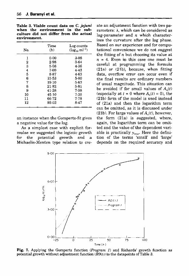
We fi t ted two curves to the d a t a of Table 3. The first curve was Richards ' model wi th a cu rv a tu r e p a r a m e t e r m = 0.25 [see Eqns (22a) and (22b)] and wi th an a d j u s t m e n t funct ion of a(t) =- 1 (i.e. An(t) =- t) to be r e l evan t to this experi- ment . Also we f i t ted the da ta by Pro- g r a m 1 as descr ibed above. The resu l t s are shown in Fig. 7. As can be seen, t he re is no problem with the goodness- of-fit in e i the r case, bu t the ext rapola- t ion to the t ime before the inocula t ion is different . This plot suggests t h a t the m a x i m u m specific growth r a t e migh t have been r eached a round or before the inoculat ion. This is also an example of

56 J. Baranyi et al.

Table 3. Viable c o u n t data on C. jejuni w h e n the e n v i r o n m e n t in the sub- cu l ture did not differ f rom the actual e n v i r o n m e n t .

Time Log counts No. (h) (loglo m1-1)

1 0.00 3.08 2 2-98 3.64 3 5.08 4.36 4 7.00 4.43 5 8.87 4.63 6 15.53 5.00 7 19-10 5-63 8 21.82 5-81 9 41.28 7.08

10 45.10 7.35 11 66.72 7.78 12 93-O2 8.47

an instance when the Gompertz-fit gives a negative value for the lag.

As a simplest case with explicit for- mulae we suggested the logistic growth for the potential growth and a Michaelis-Menten type relation to cre-

ate an adjustment function with two pa- rameters: A, which can be considered as lag-parameter and n which character- izes the curvature af ter the lag phase. Based on our experience and for compu- tational convenience we do not suggest the fitting of n but choosing its value at n = 4. Even in this case one must be careful at programming the formula (21a) or (21b), because, when fitting data, overflow error can occur even if the final results are ordinary numbers of usual magnitude. This situation can be avoided if for small values of An(t) (especially at t = 0 where An(t) = 0), the (21b) form of the model is used instead of (21a) and then the logarithm term can be omitted, as it is discussed under (21b). For large values of A,(t), however, the form (21a) is suggested, where, again, the logarithm term can be omit- ted and the value of the dependent vari- able is practically Ym~. Here the defini- tion of the terms 'small' and 'large' depends on the required accuracy and

g 8 _o

9.00

6.00

3 .00

/ !

J

.:,""/ I 0

- - RO(t}

........ Progrom I

0.00 I 1 I -25 25 50 75 I00

Time (h) Fig. 7. Applying the Gompertz function (Program 1) and Richards' growth function as potential growth without adjustment function (RO(t)) to the datapoints of Table 3.

Bacterial growth model 57

on the limit of number-representa t ion of the given computer.

A more complicated version of the new model can be obtained by (22a) and (22b), which contains two curvature pa- rameters , n and m. However, the fitting of these curvature parameters is not easy and can cause computational prob- lems. This is why we fixed their value as n = 4 and m = 1 which seemed to be a good compromise between the goodness- of-fit and convenience. This simplest version of our model contains the follow- ing parameters:

logari thm of the inoculum, Yo; lag-parameter, A; potential maximum growth rate, ~m~;

logari thm of the maximum population density, y ~ .

which represent the main characteris- tics of a sigmoid curve.

Examinat ion of non-autonomous growth models is a developing field in population theory (see for example, Vance 1990). They seem especially use- ful when modelling the adjus tment of the population to changing (or new) environment (Coleman 1978). In this paper we showed a possible way to apply this theory in food microbiology.

Acknowledgement

The authors thank the referees for sev- eral helpful suggestions.

References Baranyi, J., Roberts, T. A. and McClure, P. (1992). Theorems on a non-autonomous growth

model describing the adjustment of the bacterial population to a new environment. Sixth IMA Conference on the Mathematical Theory of the Dynamics of Biological Systems, Ox- ford, 1-3 July, 1992.

Barford, J. P., Pamment, N. B. and Hall, R. J. (1982). Lag phases and transients. In Mi, ro- bial population dynamics. (Ed Bazin, M.). CRC Press, pp. 55-91. Boca Raton, FL.

Buchanan, R. L. and Cygnarowicz, M. L. (1990) A mathematical approach toward defining the duration of the lag phase. Food Microbiol. 7, 237-240.

Coleman, B. D. (1978) Nonautonomous logistic equations as models of the adjustment of pop- ulations to environmental change. Math. Biosci. 45, 159-173.

France, J. and Thornley, J. H. M. (1984) Mathematical models in agriculture. Butterworth. Oxford.

Frederickson, A. G., Ramkrishna, D. and Tsuhiya, H. M. (1967). Statistics and dynamics of procaryotic cell populations. Math. Biosci. 1,327-374.

Gibson, A. M., Bratchell, N. and Roberts, T. A. (1988). Predicting microbial growth: growth responses of salmonellae in a laboratory medium as affected by pH, sodium chloride and storage temperature. Int. J. Food Microbiol. 6, 155-178.

Kono, T. (1968) Kinetics of microbial cell growth. Biotech. Bioeng. 10, 105-131. Korn, G. and Korn, T. (1973). Mathematical handbook for scientists and engineers. New

York. McGraw-Hill. MacDonald, N. (1978). Time lags in biological models. Berlin. Springer. Pirt, S. J. (1975). Principles of microbe and cell cultivation. London. Blackwell. Press, W. H., Flannery, B. P., Teukolsky, S. A. and Vetterling, W. T. (1990) Numerical

recipes. Cambridge. Cambridge University Press. Roels, J. A. and Kossen, N. W. F. (1978). On the modelling of microbial metabolism. In

Progress in industrial microbiology, vol. 14. (Ed. Bull, M. J.), pp. 95-203. Amsterdam. Elsevier.

Turner, M. E., Bradley, E. L., Kirk, K. A. and Pruitt, K. M. (1976). A theory of growth. Math. Biosci. 29, 367-373.

Vance, R. R. (1990) Population growth in a time-varying environment. J. Theor. Biol. 3'/, 438-454.

58 J. Baranyi et al.

Vance, R. R. and Coddington, E. A. (1989) A nonautonomous model of population growth. J. Math. Biol., 27, 491-506.

Whiting, C. (1992) Letter to the editor. Food Microbiol. 9(2), 173-174. Zwietering, M. H., Jongenburger, I., Rombouts, F. M. and van't Riet, K. (1990) Modelling of

the bacterial growth curve. Appl. Environ. Microbiol. 56, 1875-1881.

A P P E N D I X Below we s u m m a r i z e some m a t h e m a t i c a l t heo rems on the new model. Thf~se theo- r ems were p r e se n t ed in B a r a n y i e t al. (1992).

Cons ider the ini t ial va lue problem ( la) , ( lb). The theo rems below are val id also if we consider the case of l imi ted g rowth ra te , so ins tead of condit ion (c) u n d e r ( la) , ( lb) we suppose the much weake r cons t ra in t :

dtL /dx is l imited (0 < x < xm~).

Theorem 1

Let a(t) be an a d j u s t m e n t funct ion as def ined u n d e r (2a), (2b). Th en the solut ion of the ini t ial va lue problem (2a) and (2b) is

g(t) = f(A(t)), where

t

A(t) = f a(s)ds o

Theorem 2

Le t a(t) and fl(t) a d j u s t m e n t funct ions and let g~(t), go(t) denote the respect ive solut ions of (2a), (2b). I f t

I f (~(s) - fl (s))dsr < 0

t h en

Ig~(t) -go(t) l < ell~(x)xl,~ < et~(Xo)Xm~.

Let the a d j u s t m e n t funct ion have the form

t n an(t) =

A n + t n

for some A,n > O. In this ease

An(t) = ~j ~ = -ff , 0

where t f l

Bn(t)= l + s n d s . 0

Bacterial growth model 59

Theorem 3

I f n > 1 t h e n the i m p r o p r i u s i n t eg ra l

B , = l im Bn(t) t - - ~

exists . Moreove r i f n - o ~ t h e n Bn ~ 1.

Theorem 4

I f n ~oo t h e n B~(t) ~ B~(t) un i fo rmly on (0,~) whe re

t (t < 1) B~(t) =

1 (t > 1)"

Consequence : i f n ~oo t h e n A,( t ) -o A~(t) un i fo rmly on (0,~), whe re

0 (t < n) A~(t) =

t - k (t >_ h)"

Theorem 5

Using the no ta t ions above: if n - - ~ t h e n

IgA~(t)) ~ f(A~(t)) un i fo rmly on (0,~).