Barabasi Radiation Supp Inf - The University of...

Contents:

1 Datasets

1.1 US commuting

1.2 US migrations

1.3 US Commodity flow

1.4 Mobile phone database

1.5 Call patterns

2 The radiation model: analytical results

3 The case of uniform population distribution

4 Asymptotic limits

5 Determination of the gravity law’s parameters

6 Relationship between the gravity law and the radiation model

7 Differences between the Radiation model and other decision-based models

8 Self-similarity in human mobility

9 Beyond the radiation model

SUPPLEMENTARY INFORMATIONdoi:10.1038/nature

WWW.NATURE.COM/NATURE | 1

�

1 Datasets

1.1 US commuting

Data on commuting trips between United States counties are available online at

http://www.census.gov/population/www/cen2000/commuting/index.html.

The files were compiled from Census 2000 responses to the long-form (sample) questions

on where individuals worked. The files provide data at the county level for residents of

the 50 states and the District of Columbia (DC). The data contain information on

34,116,820 commuters in 3,141 counties.

1.2 US migrations

United States population migration data for 2007-2008 are available online at

http://www.irs.gov/taxstats/article/0,,id=212695,00.html.

The main source of area-to-area migration data in the United States is the Statistics of

Income Division (SOI) of the Internal Revenue Service (IRS), which maintains records of

all individual income tax forms filed in each year. The Census Bureau is allowed access

to tax returns, extracted from the IRS Individual Master File (IMF), which contains

administrative data collected for every Form 1040, 1040A, and 1040EZ processed by the

IRS. Census determines who in the file has, or has not, moved. To do this, first, coded

returns for the current filing year are matched to coded returns filed during the prior year.

The mailing addresses on the two returns are then compared to one another. If the two

are identical, the return is labeled a “non-migrant.” If any of the above information

changed during the prior 2 years, the return is considered a mover.

SUPPLEMENTARY INFORMATIONRESEARCHdoi:10.1038/nature


�

1.3 US Commodity flow

FAF3 data on commodity flow are available online at the following website

http://ops.fhwa.dot.gov/freight/freight_analysis/faf/index.htm.

The Freight Analysis Framework (FAF) integrates data from a variety of sources to

create a comprehensive picture of freight movement among US states and major

metropolitan areas by all modes of transportation. With data from the 2007 Commodity

Flow Survey and additional sources, FAF version 3 (FAF3) provides estimates for

tonnage and value, by commodity type, mode, origin, and destination for 2007.

The data consists on 5,712,385 total tonnage shipped among 123 states and Major

Metropolitan Areas (MMA).

1.4 Mobile phone database

We used a set of anonymized billing records from a European mobile phone service

provider29,30,31. The records cover over 10M subscribers within a single country over 4

years of activity. Each billing record, for voice and text services, contains the unique

anonymous identifiers of the caller placing the call and the callee receiving the call; an

identifier for the cellular antenna (tower) that handled the call; and the date and time

when the call was placed. Coupled with a dataset describing the locations (latitude and

longitude) of cellular towers, we have the approximate location of the caller when placing

the call. In order to understand whether the radiation model could also describe hourly

trips in addition to commuting trips, we analyzed the phone data during a period of six

months, recording the locations of users between 7am to 10pm. As the cell phone



�

company’s market share is not uniform across the country, in order to have the necessary

demographic information we use municipalities and not cell towers as locations. We

define a trip from municipality i to municipality j if we recorded the same user in

municipality i at time t and in municipality j at time t+1, where t is a daytime one-hour

time interval (i.e. t = 7, 8, …, 21, 22). We aggregated all trips from hour t to hour t+1

observed during the six-month period, generating the hourly commuting flows among

municipalities.

1.5 Call patterns

Using the mobile phone database described above, we also extracted the number of phone

calls between users living in different municipalities during the same period, resulting in

a total of 38,649,153 calls placed by 4,336,217 users.

2 The radiation model: analytical results

Here we propose a more general description of the radiation model, which is completely

equivalent to the formulation given in the main text. We use an analogy with radiation

emission and absorption processes, widely studied in physical sciences32. Imagine the

location of origin, i, as a source emitting an outgoing flux of identical and independent

units (particles). We define the emission/absorption process through the following two

steps:

1) We associate to every particle, X, emitted from location i a number,

!

zX(i), that

represents the absorption threshold for that particle. A particle with large threshold



�

is less likely to be absorbed. We define

!

zX(i) as the maximum number obtained after

mi random extractions from a preselected distribution, p(z) (mi is the population in

location i). Thus, on average, particles emitted from a highly populated location have

a higher absorption threshold than those emitted from a scarcely populated location.

We will show below that the particular choice of p(z) do not affect the final results.

2) The surrounding locations have a certain probability to absorb particle X:

!

zX( j )

represents the absorbance of location j for particle X, and it is defined as the

maximum of nj extractions from p(z) (remember that nj is the population in location

j). The particle is absorbed by the closest location whose absorbance is greater than

its absorption threshold.

By repeating this process for all emitted particles we obtain the fluxes across the entire

country.

We can calculate the probability of one emission/absorption event between any two

locations, and thus obtain an analytical prediction for the flux between them. Let

!

P(1 |mi,n j ,sij ) be the probability that a particle emitted from location i with population mi

is absorbed in location j with population nj, given that sij is the total population in all

locations (except i and j) within a circle of radius rij centered at i (rij is the distance

between i and j). According to the radiation model, we have

!

P(1 |mi,n j ,sij ) = dz Pmi(z)Ps ij (< z)Pn j

(> z)0

"

# (S1)

where

!

Pmi(z) is the probability that the maximum value extracted from p(z) after mi trials

is equal to z:

!

Pmi(z) =

dPmi(< z)dz

= mip(< z)mi "1 dp(< z)

dz.



�

Similarly,

!

Psij (< z) = p(< z)sij is the probability that sij numbers extracted from the

!

p(z)

distribution are all less than z; and

!

Pn j(> z) =1" p(< z)n j is the probability that among nj

numbers extracted from

!

p(z) at least one is greater than z.

Thus Eq. (S1) represents the probability that one particle emitted from a location with

population mi is not absorbed by the closest locations with total population sij, and is

absorbed in the next location with population nj. After evaluating the above integral, we

obtain

P(1 |mi,nj, sij ) =mi dz dp(< z)dz

p(< z)mi+sij!1 ! p(< z)mi+nj+sij!1"#

$%0

&

' =mi1

mi + sij!

1mi + nj + sij

"

#((

$

%))

P(1 |mi,nj, sij ) =minj

(mi + sij )(mi + nj + sij ) (S2)

Eq. (S2) is independent of the distribution

!

p(z) and is invariant under rescaling of the

population by the same multiplicative factor (njobs).

The probability P (Ti1,Ti2,...,TiL ) for a particular sequence of absorptions, (Ti1,Ti2,...,TiL ) ,

of the particles emitted at location i is given by the multinomial distribution:

!

P (Ti1,Ti2,...,TiL ) =Ti!Tij!

pijTij

j" i# with

!

Tijj" i# = Ti (S3)

where

!

Ti is the total number of particles emitted by location i, and

!

pij " P(1 |mi,n j ,sij ).

The distribution (S3) is normalized because

!

pijj" i# = mi

1(mi + sij )

$1

(mi + n j + sij )

%

& '

(

) *

j" i# =1.

The probability that exactly

!

Tij particles emitted from location i are absorbed in location j

is obtained by marginalizing probability (S3):



�

!

P(Tij |mi,n j ,sij ) = Pi(Ti1,Ti2,...,Tij ,...,TiL ){Tik :k" i, j;Tik

k"i# =Ti }

# =Ti!

Tij!(Ti $Tij )!pijTij (1$ pij )

Ti $Tij (S4)

that is a binomial distribution with average

Tij ! Ti pij = Timi nj

(mi + sij )(mi + nj + sij ) (S5)

and variance Ti pij (1! pij ) .

The proposed radiation model might provide further insights on the problem of defining

human agglomerations. For example, the US Census Bureau uses the number of

commuters between counties as the basis to define Metropolitan Statistical Areas in the

USA. Finding a practical way to define the boundaries of a city is important also because

it represents a key difficulty in understanding regularities such as Zipf’s law or Gibrat’s

Law of proportionate growth, since different definitions of cities give rise to different

results33,34.

3 The case of uniform population distribution

Comparing the radiation model, Eq. (S5), with the gravity law, Eq. (1), the most

noticeable difference is the absence of variable r, the distance between the locations of

origin and destination, and the introduction of a new variable, s, the total population

within a circle of radius r centred in the origin.

In the particular case of a uniform population distribution, however, we can perform a

change of variable and write the radiation model, Eq. (S5), as a function of the distance r,



�

as in the gravity law, Eq. (1). If the population is uniformly distributed, then

!

n = m and

!

s(r) = m"r2 and the average number of travelers is given by:

!

T(m,n,s) = mP(1 |m,n,s) =m2n

(m + s)(m + n + s)=

m(1+ s /m)(2 + s /m)

With the change of variable we get

!

T(m,n,r ) =m

(1+"r2)(2 +"r2)#mr4

, (S6)

obtaining a gravity law with

!

f (r) = r" ,

!

" = 4 and

!

" + # =1, which is the same form as

the one chosen in Ref. 14, although the value of parameters !," and ! are different.

However, it is important to note that the assumption of uniform population distribution

used to derive Eq. (S6) is not fulfilled in reality, as can be seen in Fig. S1, where we plot

the distribution of exponents

!

µ , obtained by fitting the data with

!

s(r)" rµ for

!

r <119km. The mean value (with a large variance) is found to be µ = 2.53 and not 2, as

we would expect for a uniform spatial population distribution. Therefore a gravity law

with

!

f (r) = r" cannot be derived from that argument, and thus there is no reason to prefer

it to other functions with an equal number of free parameters that can provide a

comparable agreement with the data (one commonly used version is for example11

f (r) = edr ). We will show in Section 6 that from the radiation model it is possible to

derive the gravity law in Eq. (S6) under weaker assumptions on the population

distribution.

The variable s, also called rank, has been previously recognized as a relevant quantity in

different mobility and social phenomena: it has been first introduced in the intervening

opportunity model26 to describe migrations (see SI sect. 7), and recently it has found



�

applications in the study of social-network friendship35, and in the analysis of urban

movements of Foursquare’s users in different cities36.

4 Asymptotic limits

In order to test the analytic self-consistency of the gravity and radiation models it is

instructive to calculate the asymptotic limits on the number of trips when the populations

in the origin or destination increase. Consider for example the case in which the

population of the origin location, m, becomes very large compared to n and s (

!

m >> n,s).

The gravity law (1) predicts that the number of trips, T, will diverge to infinity. This is

not realistic, because the location of destination cannot offer jobs to an unlimited number

of commuters. On the contrary, the radiation model, Eq. (S4), predicts that the number of

travelers saturates at

!

Tm"# = n +O1m2

$

% &

'

( ) , and that the other commuters will travel to

farther locations.

The inconsistency of the gravity law is even more evident when we consider the limit of

large population in the location of destination (

!

n >> m,s). Again Eq. (1) predicts that the

number of trips, T, will increase without limit, which is impossible considering that the

population in the origin is unchanged and the number of commuters cannot exceed the

total population. The radiation model, instead, predicts that the number of travelers

saturates at

!

Tn"# =m2

(m + s)+O 1

n$

% & '

( ) * m .

These considerations provide further support to our thesis that any form of the gravity

law (1) is inherently inappropriate to satisfactorily describe commuting fluxes.



�

5 Determination of the gravity law’s parameters

Here we describe the method that we used to find the best values for the gravity law

parameters. The gravity law assumes that the average number of travelers between two

locations,

!

TijGM , can be expressed as a function of the two populations and the distance as

!

TijGM = C

mi"n j

#

rij$ . Taking the logarithm on both sides we obtain

!

ln(TijGM ) = ln(C) +" ln(mi) + #ln(n j ) $ % ln(rij ) . It is then customary in many studies to use

!

lnTijdata , the logarithm of the number of travelers in the data, to estimate the values of

!

lnC,",#,$ through a least-squares regression analysis1.

In order to obtain more accurate results, following Ref. 14 we use a nine-parameter form

of the gravity law, in which short and long trips are fitted separately. The parameters are

two sets of

!

[C,",#,$ ], one for short and one for long trips, plus

!

" , the cutoff distance that

defines short and long trips (i.e. short if

!

rij < " , long otherwise).

We define the error function as the mean square deviation of the logarithms of trips:

!

E =1N

[ln(TijGM ) " ln(Tij

data )]2{i, j:i# j}$ , (S7)

where the sum extends over all locations pairs (i, j) such that

!

Tijdata ,Tij

GM > 0, and N is the

total number of county pairs considered. We finally select the particular set of the nine

parameters that minimizes E in Eq. (S7).

Moreover, we checked that the power law deterrence function,

!

f (rij ) = rij" , provides a

better fit compared to the exponential deterrence function, f (rij ) = edrij . Indeed, we found

!!!!!!!!!!!!!!!!!!!!!!!!!!!!!!!!!!!!!!!!!!!!!!!!!!!!!!!!1!As pointed out in Ref. 37 there are other ways to determine the values of the best-fit parameters. Here we will only consider the most widely used approach for “Newtonian” gravity laws, of the type of Eq. (1), defined above.!



�

that the best-fit parameters obtained with the power law deterrence function always

provide smaller errors E.

The sensitivity of the gravity law to the number of zero fluxes is known to be one of the

main factors to determine the quality of the gravity fit. Indeed, for freight transportation,

in which the gravity law provides its better prediction, 97.5% of all possible pairs of

locations have a non-zero flux, compared to 3.2% of phone calls, 1.65% of commuting

fluxes, and 0.8% of migrations.

6 Relationship between the gravity law and the radiation model

To understand the relationship between the gravity law and the radiation model, let us

assume, in line with our empirical observations, that the radiation model provides a good

approximation to the data, i.e.

!

Tijdata " Tij

Rad =mi2n j

(mi + sij )(mi + n j + sij ). To identify the

conditions under which the gravity law also offers a good fit to the data, let us minimize

the following error function:

!

E =1N

ln Cmi

"n j#

rij$

%

& ' '

(

) * * + ln

mi2n j

(mi + sij )(mi + n j + sij )

%

& ' '

(

) * *

,

- . .

/

0 1 1

2

{i, j:i2 j}3 , (S8)

i.e. determine the conditions (and the values of

!

[", #, $ ]) under which the mean square

deviation between gravity’s and radiation’s predictions is minimized.

We can write the variables

!

mi and

!

n j as deviations from the local average population,

!

m " (mi + n j + sij ) /Nij , where

!

Nij is the number of locations in a circle of radius rij

centered in i (rij is the distance between i and j), and

!

(mi + n j + sij ) is the total population



�

in these locations. We have

!

mi = m (1+" i) and

!

n j = m (1+" j ) , with

!

" i =mi #m

m and

!

" j =n j #m

m . Equation (S7) then becomes (!2 =1/C )

E = 1N

lnm!+" (1+#i )

! (1+# j )"

$2rij%

!

"##

$

%&&' ln

m3(1+#i )2 (1+# j )

m2Nij (Nij '1'# j )

!

"##

$

%&&

(

)**

+

,--

2

{i, j:i. j}/ .

E reaches its minimum, resulting in a better fit, if each element in the sum is close to

zero:

(! +" !1)ln(m)+ (! ! 2)ln(1+#i )+ (" !1)ln(1+#i )! ln($2rij

% )+ ln(Nij )+ ln(Nij !1!# j ) = 0 for all

!

{i, j : i " j} .

This is true if the following conditions are satisfied:

(! +" !1)ln(m) = 0 " ! +" =1 (i)

(! ! 2)ln(1+"i )+ (# !1)ln(1+" j ) = 0 " (! ! 2)"i + (# !1)" j # 0 (ii)

ln(Nij )+ ln(Nij !1!!ij )! ln("2rij

# ) = 0" ln(Nij / "rij# /2 )! ln[(Nij !1!!ij ) / "rij

# /2 ]= 0" "rij# /2 # Nij

(iii)

Equation (i) reproduces the result we obtain if we derive the gravity law from the

radiation model in the limit of constant population density. Equation (ii) is always true if

! = 2 and ! =1 , but this is in contrast with condition ! +" =1 obtained from (i) and

corresponding to the dominant contribution to E. Indeed, if the deviations of populations

from the local average are small, i.e.

!

" i," j <<1, then the contribution to E of (ii) is small

and negligible compared to ln(m) , which is the largest term if m >>1 . Condition (iii) is

satisfied for

!

" = 4 when the locations are regularly spaced or have equal area, like in a

grid. In this case

!

" can be interpreted as the global density of locations (i.e. the total

number of locations divided by the country’s area). If, on the contrary, the locations are



�

not regularly spaced, the density of locations within origin i and destination j will be

different for every pair (i, j), and thus it will be impossible to find a value for parameter

!

" that is constant throughout the country, compromising the goodness of the fit.

Thus, when locations have approximately the same area and the local deviations of

population are small, Equations (i)-(iii) give the following theoretical predictions for the

best-fit values: ! +" =1 and

!

" = 4 .

We now turn to the empirical data and show that the better Eqs. (i)-(iii) are satisfied, the

better is the gravity law’s fit. We will analyse the commuting fluxes within the United

States, for which we have empirical data at the county level (i.e. the number of

commuters between the U.S. counties), by grouping the counties into larger regions, and

aggregating the fluxes between them accordingly. In particular, we will show two

different aggregations, one that fulfils equations (i)-(iii) and one that does not, and we

will compare the performance of the gravity law in the two cases.

Locations with equal population. The locations are the congressional districts, obtained

by an appropriate aggregation of counties such that all districts have roughly the same

population (see Fig. S2). In particular, there are 435 districts with an average population

of

!

652,701±153,834 individuals. This subdivision does not fulfil equation (iii),

requiring regularly spaced locations. Indeed, as can be seen in the map of Fig. S2, the

density of locations is higher in highly populated regions, where districts’ average area is

also very small, compared to districts in low populated regions.

The gravity law’s best-fit parameters for commuting trips at the district level are

!

[", #, $ ] = [-0.31, 0.31, 2.80] for

!

r < 500 km,

!

[", #, $ ] = [-0.23, -0.33, 0.14] for

!

r > 500 km, that do not fulfill the conditions ! +" =1 and

!

" = 4 obtained by equations



�

(i)-(iii). It is interesting to note that

!

" and

!

" are sometimes negative, meaning that when

the population increases, less travelers are predicted.

To assess the goodness of the fit we calculate the error as the mean square deviation of

the logarithms of trips,

!

E =1N

[ln(TijGM ) " ln(Tij

data )]2{i, j:i# j}$ , where the sum extends over all

locations pairs (i, j) such that

!

Tijdata ,Tij

GM > 0, and N is the total number of county pairs

considered. In this case the error Edistrict is 1.43.

Locations with equal area. The locations are defined by placing on the U.S. map a square

grid, and grouping together all counties whose geometrical centroids lie within the same

square. In this way we obtain 400 equally spaced locations having roughly the same area,

as can be seen in Fig. S3; the average area is

!

19,160 ± 8,658 km2. This subdivision thus

fulfils the requirement of equally spaced locations, necessary for Eq. (iii) to hold. The

gravity law’s best-fit parameters for commuting trips are

!

[", #, $ ] = [0.48, 0.58, 4.35]

for

!

r < 390 km,

!

[", #, $ ] = [0.40, 0.33, 0.49] for

!

r > 390, that are compatible with the

conditions ! +" =1 and

!

" = 4 given by equations (i)-(iii) when

!

r < 390 km (where 95%

of trips takes place). When

!

r > 390 km the best fit parameters do not agree with our

estimates, due to the difficulty to predict the small fraction of long-distance trips, as

discussed in the main text. The error is Egrid = 0.96, smaller than in the previous case,

confirming that the gravity law works better when locations have equal area and are

equally spaced, and as long as there is a local uniformity in the population distribution.

This result is also an indirect validation of the radiation model, because in order to obtain

the conditions ! +" =1 and

!

" = 4 that agree with the experimental values, we assumed

!

Tijdata " Tij

Rad .



�

7 Differences between the Radiation model and other decision-based models.

The Radiation model’s approach is similar to the original idea behind the intervening-

opportunities model26,38, but the developments and the final results and performances are

radically different.

The intervening-opportunities (IO) model proposes that “the number of persons going a

given distance is directly proportional to the number of opportunities at that distance and

inversely proportional to the number of intervening opportunities”26. Assuming that the

number of opportunities in a location is proportional to its population, we have that the

number of trips between locations i and j is Tij !nj (sij +mi ) where nj is population in

location j and (sij + mi) is the population in all locations between i and j. In Fig. S5 we

show the performance of Stouffer’s IO model tested on US commuting fluxes.

This first formulation was subsequently recast in a stochastic approach that has become

the standard theory of IO models, and it is defined as follows38: the probability that a trip

will terminate in location j is equal to the probability that j contains an acceptable

destination and that an acceptable destination closer to the origin i has not been found.

The number of trips is shown to be Tij ! e"! (sij+mi )"

" e"! (sij+mi+nj )"#

$%& , where e!! is the

probability that a single opportunity is not sufficiently attractive as destination, and !

and ! are fitting parameters.

The IO model shares with the radiation model the intuition of using distance to sort the

possible destinations, identifying that the correct variable to calculate Tij is sij and not rij

as used in the gravity law. Besides this, the IO model suffers from problems that are

similar to those highlighted earlier for the gravity law. In particular, the lack of universal

values for parameters ! and ! , and the difficulty to calibrate these values makes



�

impossible to obtain the correct number of total trips28,39,40. These shortcomings, along

with a higher computational complexity, have led to the success of the gravity law over

the IO model in recent years40.

Another decision-based approach is the random utility (RU) model27,41. In RU models,

utilities distributed according to a logit-function are assigned to each destination. Utilities

can depend on various variables including travel times, distances, job opportunities. A

rationality paradigm is used to model the decision process: the individual will choose the

alternative that maximizes a random utility function subject to specific cost constraints.

Although RU model’s predictions can be derived from first principles, they depend on

tunable parameters that are context specific, and do not clearly outperform the gravity

law’s estimates40.

8 Self-similarity in human mobility

The radiation model helps us uncover a previously unsuspected scale-invariance in

commuting patterns. Let us denote with ps (> s |m) the probability of a trip from a

location with population m to any destination that lies beyond a circle of radius r(s)

centered at the source (i.e. a circle containing population s). The radiation model (2)

predicts that this probability has the simple form

ps (> s |m) =1

1+ s /m, (S9)

which is scale invariant under the transformation m! !m and s! !s . Such scale-

invariance is absent, however form the gravity law (1). To offer empirical evidence for

this statistical self-similarity in Fig. 4a we plot the s-dependence of ps (> s |m) for 2,000



�

US counties, the obtained curves spanning about six orders of magnitude in s. Yet, if we

plot ps (> s |m) in function of the dimensionless s/m, as predicted by (S9), the differences

between the different curves decrease significantly, and the universal function 1/(1+x)

predicted by (S9) offers a close lower bound to the rescaled curves (Fig. 4b).

!

9 Beyond the radiation model

Here we show how Eq. (2) is not a rigid end point of our approach, but can serve as a

platform that can be improved upon in specific environments. For example, the radiation

model slightly underestimates the number of very long commuting patterns (those over

1000 km, Fig. 2a and Fig. S7). While this impacts less than 1% of all trips (336,113 of

34,116,820 travelers), the agreement could be improved via an effective distance, used in

transportation modeling42, defining the variable sij as the population within an effective

travel time from the origin. Indeed, if efficient means of transport are available (like

direct flights), individuals are willing to commute farther.

As a second example we consider the fact that an individual has a home-field advantage

when searching for jobs in his/her home county, being more familiar with local

employment opportunities. This is justified considering that individuals have a better

knowledge of their home location, because they know more people, have more

connections, and thus have access to more employment opportunities than in an

unfamiliar location, where they can typically apply only to widely advertised jobs.

In the radiation model we implement this home-advantage in the following way: while

for the other locations the number of job offers is proportional to the respective



�

populations, for the home location the number of job opportunities is proportional to the

population, m / n jobs +! / n jobs , which corresponds to the effective the addition of !

people. Below we show the new expressions of the probability of one trip, P(1 |m,n, s) ,

and the probability of a trip to a destination beyond a circle of radius r(s) centered at the

origin, ps (> s |m) , for the home-advantage variant described above:

P(1 |m,!,n, s) = (m+!)n((m+!)+ s)((m+!)+ n+ s)

(S10 a)

ps (> s |m,!) =(m+!)(m+!)+ s

(S10 b)

The adjusted law is now invariant under the (m+!)! "(m+!) and s! !s

transformation. This version of the radiation model, with ! = 35,000, provides a better

collapse of the rescaled distributions ps (> s |m) , as shown in Fig. 4c. In Fig. S6 we show

that the new version also provides comparable results on the prediction of p(T |m,n, r) ,

Pdist (r) , and Pdest (n) distributions, for which the original radiation model was already

over-performing the gravity model. Moreover, the better performance of the new version

is particularly evident in the pairwise comparison of real data fluxes and the radiation

model’s predictions, shown in the scatter plot of Fig. S6c (the individual points are

omitted for the sake of clarity). The error bars corresponding to the new version are

systematically shorter than the error bars of the original radiation model, indicating

smaller fluctuations of its predictions and demonstrating that Eq. (2) is not a rigid end

point of our approach, but can serve as a platform that can be improved upon in specific

environments.



�

Additional References 31 Song, C., Qu, Z., Blumm, N. & Barabási, A. L. Limits of predictability in human

mobility. Science 327, 1018 (2010). 32 Kittel, C. & McEuen, P. Introduction to solid state physics. Vol. 4 (Wiley New

York, 1986). 33 Rozenfeld, H. D., Rybski, D., Andrade, J. S., Batty, M., Stanley, H. E. & Makse,

H. A. Laws of population growth. Proceedings of the National Academy of Sciences 105, 18702 (2008).

34 Eeckhout, J. Gibrat's law for (all) cities. American Economic Review, 1429-1451 (2004).

35 Liben-Nowell, D., Novak, J., Kumar, R., Raghavan, P. & Tomkins, A. Geographic routing in social networks. Proceedings of the National Academy of Sciences of the United States of America 102, 11623 (2005).

36 Noulas, A., Scellato, S., Lambiotte, R., Pontil, M. & Mascolo, C. A tale of many cities: universal patterns in human urban mobility. Arxiv preprint arXiv:1108.5355 (2011).

37 Flowerdew, R. & Aitkin, M. A method of fitting the gravity model based on the Poisson distribution. Journal of Regional Science 22, 191-202 (1982).

38 Schneider, M. Gravity models and trip distribution theory. Papers in Regional Science 5, 51-56 (1959).

39 Whitaker, R. W. & West, K. E. The intervening opportunities model: a theoretical consideration. Highway Research Record (1968).

40 Heanue, K. E. & Pyers, C. E. A comparative evaluation of trip distribution procedures. Highway Research Record (1966).

41 McFadden, D. Modelling the choice of residential location. (Institute of Transportation Studies, University of California, 1978).

42 Kurant, M. & Thiran, P. Extraction and analysis of traffic and topologies of transportation networks. Physical Review E 74, 036114 (2006).



�

Figure S1

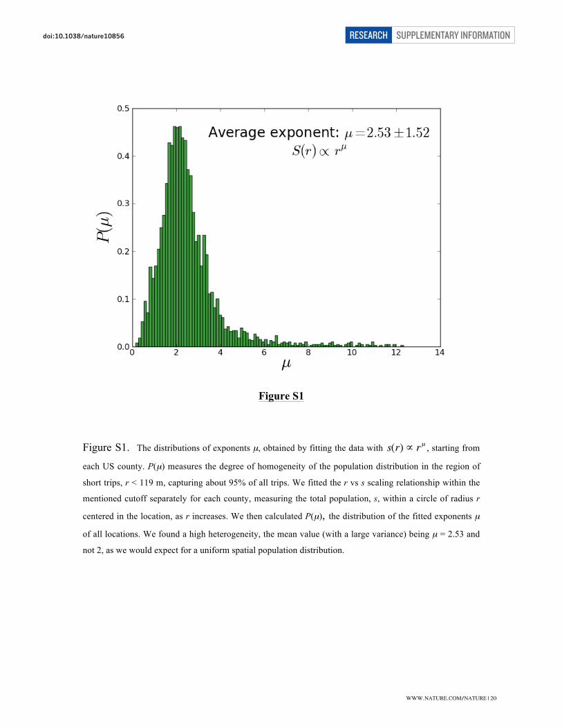
Figure S1. The distributions of exponents µ, obtained by fitting the data with

!

s(r)" rµ , starting from

each US county. P(µ) measures the degree of homogeneity of the population distribution in the region of

short trips, r < 119 m, capturing about 95% of all trips. We fitted the r vs s scaling relationship within the

mentioned cutoff separately for each county, measuring the total population, s, within a circle of radius r

centered in the location, as r increases. We then calculated P(µ), the distribution of the fitted exponents µ of all locations. We found a high heterogeneity, the mean value (with a large variance) being µ = 2.53 and

not 2, as we would expect for a uniform spatial population distribution.



�

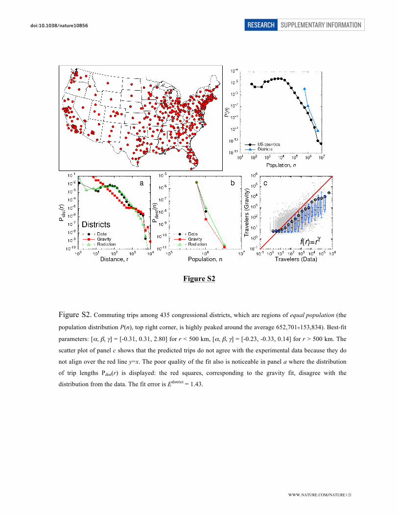
Figure S2

Figure S2. Commuting trips among 435 congressional districts, which are regions of equal population (the

population distribution P(n), top right corner, is highly peaked around the average 652,701±153,834). Best-fit

parameters: [α, β, γ] = [-0.31, 0.31, 2.80] for r < 500 km, [α, β, γ] = [-0.23, -0.33, 0.14] for r > 500 km. The

scatter plot of panel c shows that the predicted trips do not agree with the experimental data because they do

not align over the red line y=x. The poor quality of the fit also is noticeable in panel a where the distribution

of trip lengths Pdist(r) is displayed: the red squares, corresponding to the gravity fit, disagree with the

distribution from the data. The fit error is Edistrict = 1.43.



�

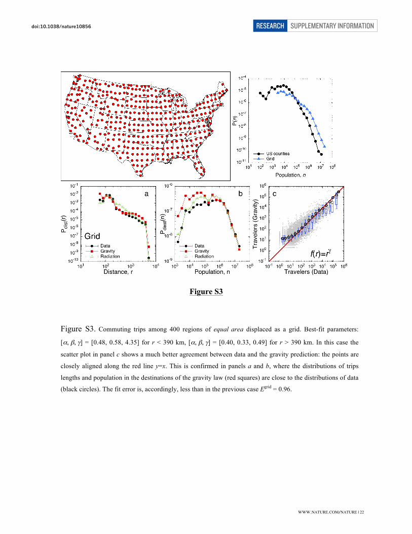
Figure S3

Figure S3. Commuting trips among 400 regions of equal area displaced as a grid. Best-fit parameters:

[α, β, γ] = [0.48, 0.58, 4.35] for r < 390 km, [α, β, γ] = [0.40, 0.33, 0.49] for r > 390 km. In this case the

scatter plot in panel c shows a much better agreement between data and the gravity prediction: the points are

closely aligned along the red line y=x. This is confirmed in panels a and b, where the distributions of trips

lengths and population in the destinations of the gravity law (red squares) are close to the distributions of data

(black circles). The fit error is, accordingly, less than in the previous case Egrid = 0.96.



�

Figure S4

Figure S4. The number of emitted particles, Ti ! Tijj"i# , versus the population of each location,

!

mi .

The assumption

!

Ti " mi is verified for all cases except for freight transportation and phone data, because

the weight of commodities produced in a region is not related to the region’s population, and the cell phone

company’s market share is not uniformly distributed in the country. For these two cases we used the

measured

!

Ti .



�

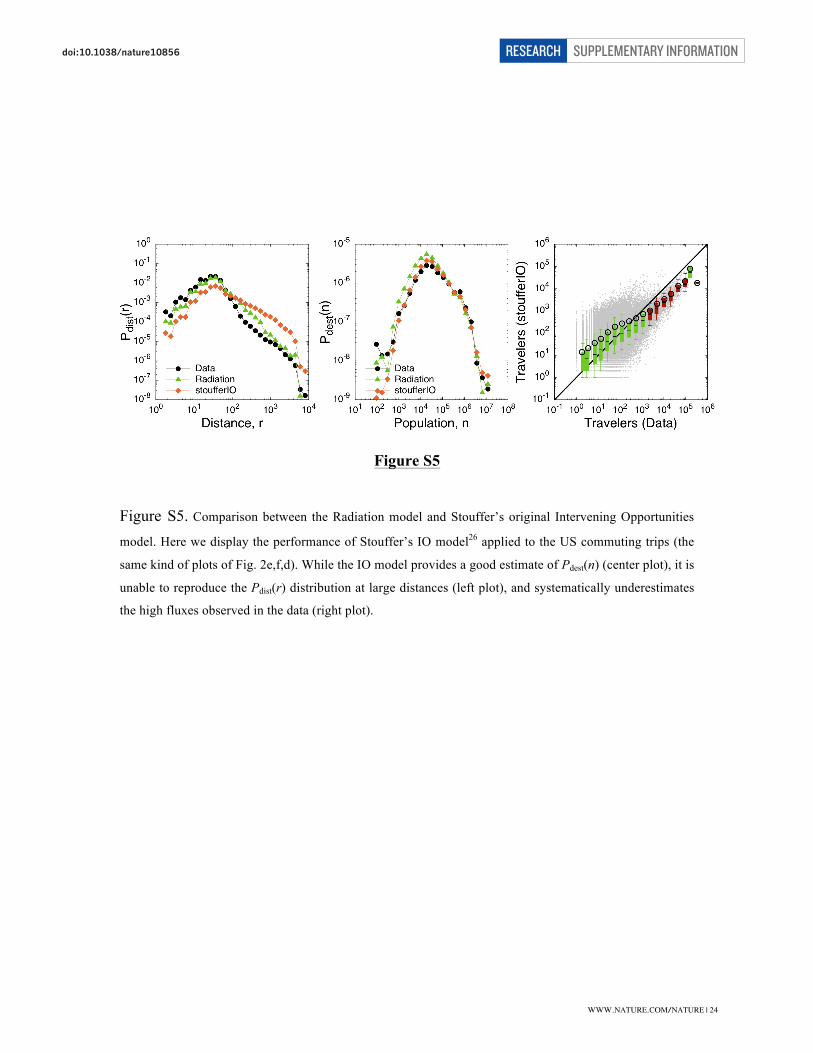
Figure S5

Figure S5. Comparison between the Radiation model and Stouffer’s original Intervening Opportunities

model. Here we display the performance of Stouffer’s IO model26 applied to the US commuting trips (the

same kind of plots of Fig. 2e,f,d). While the IO model provides a good estimate of Pdest(n) (center plot), it is

unable to reproduce the Pdist(r) distribution at large distances (left plot), and systematically underestimates

the high fluxes observed in the data (right plot).



�

Figure S6

Figure S6. Variant of the radiation model. See section 9, and Fig. 2.



�

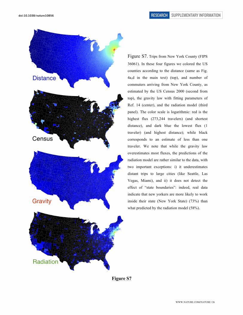
Figure S7. Trips from New York County (FIPS

36061). In these four figures we colored the US

counties according to the distance (same as Fig.

4a,d in the main text) (top), and number of

commuters arriving from New York County, as

estimated by the US Census 2000 (second from

top), the gravity law with fitting parameters of

Ref. 14 (center), and the radiation model (third

panel). The color scale is logarithmic: red is the

highest flux (273,244 travelers) (and shortest

distance), and dark blue the lowest flux (1

traveler) (and highest distance); while black

corresponds to an estimate of less than one

traveler. We note that while the gravity law

overestimates most fluxes, the predictions of the

radiation model are rather similar to the data, with

two important exceptions: i) it underestimates

distant trips to large cities (like Seattle, Las

Vegas, Miami), and ii) it does not detect the

effect of “state boundaries”: indeed, real data

indicate that new yorkers are more likely to work

inside their state (New York State) (73%) than

what predicted by the radiation model (58%).

Figure S7



�

Figure S8 Figure S8. Commuting landscapes. The commuting-based attractiveness of various US counties as seen from the perspective of an individual in (a-c) Clayton County, GA, and (d-f ) Davis County, UT. (a,d) Distance of all US counties from Clayton county, GA, in (a), and Davis county, UT, in (d). Each square represents a county, whose color denotes the distance from Clayton (Davis) county and the size is proportional to the county’s area. Seven large cities are shown to guide the eye. b,c (e,f ), The distance of counties relative to Clayton, GA (Davis, UT) has been altered to reflect the likelihood that an individual from Clayton (Davis) county would commute to these, as predicted by (2). Big cities appear much closer than suggested by their geographic distance, due to the many employment opportunities they offer. For the UT-based individual the US seems to be a “smaller” country, than for the GA-based individual. Indeed, given the low population density surrounding Davis county, the employee must travel far to satisfy his/her employment needs. Equally interesting is the fact that the Clayton county, GA, based individual sees an effective employment “hole” in its vicinity (c). The reason is the nearby Atlanta, which offers so many employment opportunities, that all other counties become far less desirable.



Barabasi Radiation Supp Inf - The University of...

Documents

Transcript of Barabasi Radiation Supp Inf - The University of...