BANKS’ PRICING STRATEGIES ANDINCOME DIVERSIFICATION: THEORETICAL

AND EMPIRICAL EVIDENCE

Thesis submitted for the degree of

Doctor of Philosophy

at the

University of Leicester

byCaner Gerek

School of ManagementUniversity of Leicester

June 2016

Banks’ Pricing Strategies and Income Diversification:Theoretical and Empirical Evidence

byCaner Gerek

Abstract

This thesis makes three different contributions to the literature on bank incomediversification and its effect on bank performance. Firstly, the study makes a theo-retical contribution by incorporating non-interest income components into Ho andSaunders (1981) model in the presence of pricing strategies, including bundling andloss-leader strategies, as well as being well-informed and less-informed customers.The model distinguishes fees and commissions income and trade income by propos-ing the conditions that create the negative relationships with net interest margin.The study also empirically tests the theoretical relationships for the European bank-ing system and the results state that both fees and commissions income and tradeincome negatively affect interest margin.

Secondly, this study examines the relationship between interest and non-interestincome sides by considering the switching cost for customers created by loan ma-turity for non-interest products. Theoretically, the study derives an equation thatlong-term loans create a switching cost for the sale of non-traditional products.The theoretical contribution is empirically tested for the UK banking system usingunique UK banking data over the period 2005 - 2012. The empirical results suggestthat by shifting loan maturity from short term to long term creates a switching costfor non-interest product sale. This empirical finding leads to test switching costcreated by long-term loan, particularly for trade products. Shifting the maturityfrom short term to long term creates switching cost for trade products either.

Thirdly the study contributes by investigating the aftermath of findings on therelationship between interest and non-interest income sides, and switching cost cre-ated by increasing loan maturity. The third study in this thesis contributes to theliterature by examining the effect of non-interest income, conditional on deposit andloan maturities, on bank performance using UK banking data as a laboratory from2005 to 2012. The study finds that fees and commissions income do not explain bankperformance. However, when the fees and commissions variables are conditional onlonger loan maturity, it alleviates the risk-adjusted bank performance. Trade in-come increases the bank performance. However when it is dependent on depositsand loans with long maturities, it has an adverse effect on bank performance. Theresult of direct maturity diversification indicates that, while the UK banks do notbenefit from deposit diversification, the maturity diversification of loan is linked toa higher bank performance.

i

Acknowledgement

All praise is due to Allah, who has made it possible for me to complete this pro-gramme despite all odds.

First and foremost, I would like to thank my supervisors Dr Mohammed Shabanand Prof Meryem Duygun for their continued support throughout my studies, pro-viding me with the flexibility, inspiration and guidance to develop as a researcher.I am most grateful for their advice, constructive comments and willingness to sharetheir views and knowledge. I have gained invaluable experience.

I am extremely grateful to Ministry of National Education of Turkey for theirfunds to provide opportunity to undertake my thesis.

I am greatly indebted to my beloved wife Zeynep Gerek. Without her love,patience, continuous support and encouragement, this would not have been possible.I am also greatly indebted to my grandfather Mehmet Sofuoglu who always proudof me. Without a shadow, my grandfather was one of the most influential persons inmy life. I am eternally thankful to my parents, Mrs Kadriye Gerek and Mr. HidayetGerek, and my sister Esra Goktepe.

Finally, I would like to thank my friends Dr Sencer Selcuk, Dr Ayse Demir Ulku,Dr Gultekin Gollu, Dr Serhat Yuksel, Dr Burhan Alveroglu, Dr Ahmet MithatTuncez, Cem Onur Karatas, Hakan Bingol, Nurullah Usta and Israfil Boyaci. Theirinvaluable assistance, warm friendship and support will always be remembered. Ona personal note, I extend my thanks to some of my closest acquaintances, AdnanAyna, Fatih Kansoy, Hasan Basak, Resul Haser, Gokmen Durmus and Yusuf Nartfor all their cooperation and moral support. All these wonderful friends have madea significant difference in my life; it is of great comfort to know that their help is athand.

ii

Contents

1 Introduction 11.1 Objectives . . . . . . . . . . . . . . . . . . . . . . . . . . . . . . . . . 51.2 Motivations . . . . . . . . . . . . . . . . . . . . . . . . . . . . . . . . 61.3 Contribution of the Research . . . . . . . . . . . . . . . . . . . . . . . 71.4 Organisation of the Thesis . . . . . . . . . . . . . . . . . . . . . . . . 8

2 The Effect of Trade and Fee Income on Net Interest Income:Theoretization of Bundling Strategies 102.1 Introduction . . . . . . . . . . . . . . . . . . . . . . . . . . . . . . . . 112.2 Literature . . . . . . . . . . . . . . . . . . . . . . . . . . . . . . . . . 14

2.2.1 Literature on Net Interest Margin . . . . . . . . . . . . . . . . 142.2.2 Literature on Bundling . . . . . . . . . . . . . . . . . . . . . . 19

2.3 Theoretical Model . . . . . . . . . . . . . . . . . . . . . . . . . . . . . 222.3.1 Assumptions and Scenarios . . . . . . . . . . . . . . . . . . . 222.3.2 Maximizations . . . . . . . . . . . . . . . . . . . . . . . . . . . 32

2.4 Data . . . . . . . . . . . . . . . . . . . . . . . . . . . . . . . . . . . . 412.5 Variables . . . . . . . . . . . . . . . . . . . . . . . . . . . . . . . . . . 42

2.5.1 Dependent Variable . . . . . . . . . . . . . . . . . . . . . . . . 432.5.2 Explanatory Variables: . . . . . . . . . . . . . . . . . . . . . . 44

2.6 Methodology for Empirical Study . . . . . . . . . . . . . . . . . . . . 492.7 Results . . . . . . . . . . . . . . . . . . . . . . . . . . . . . . . . . . . 542.8 Conclusion . . . . . . . . . . . . . . . . . . . . . . . . . . . . . . . . . 592.9 Appendix A . . . . . . . . . . . . . . . . . . . . . . . . . . . . . . . . 62

3 Switching Cost Effect of Long-term Loan in Cross Selling 673.1 Introduction . . . . . . . . . . . . . . . . . . . . . . . . . . . . . . . . 683.2 Literature Review . . . . . . . . . . . . . . . . . . . . . . . . . . . . . 703.3 Theoretical Model . . . . . . . . . . . . . . . . . . . . . . . . . . . . . 74

3.3.1 Kim’s Model . . . . . . . . . . . . . . . . . . . . . . . . . . . 743.3.2 Present Value Maximization . . . . . . . . . . . . . . . . . . . 793.3.3 Non-interest Income Side - Loanavity Effect . . . . . . . . . . 83

3.4 Data . . . . . . . . . . . . . . . . . . . . . . . . . . . . . . . . . . . . 873.5 Variables . . . . . . . . . . . . . . . . . . . . . . . . . . . . . . . . . . 89

3.5.1 Dependent Variables . . . . . . . . . . . . . . . . . . . . . . . 893.5.2 Theoretical Explanatory Variables . . . . . . . . . . . . . . . . 903.5.3 Non-theoretical Explanatory Variables . . . . . . . . . . . . . 92

3.6 Methodology for Empirical Study . . . . . . . . . . . . . . . . . . . . 933.7 Results . . . . . . . . . . . . . . . . . . . . . . . . . . . . . . . . . . . 943.8 Conclusion . . . . . . . . . . . . . . . . . . . . . . . . . . . . . . . . . 99

iii

3.9 Appendix B . . . . . . . . . . . . . . . . . . . . . . . . . . . . . . . . 102

4 Bank Performance Effect of Deposit and Loan Maturities 1034.1 Introduction . . . . . . . . . . . . . . . . . . . . . . . . . . . . . . . . 1044.2 Literature Review . . . . . . . . . . . . . . . . . . . . . . . . . . . . . 1074.3 Portfolio Theory . . . . . . . . . . . . . . . . . . . . . . . . . . . . . 1134.4 Data . . . . . . . . . . . . . . . . . . . . . . . . . . . . . . . . . . . . 1164.5 Variables . . . . . . . . . . . . . . . . . . . . . . . . . . . . . . . . . . 117

4.5.1 Dependent Variables . . . . . . . . . . . . . . . . . . . . . . . 1174.5.2 Explanatory Variables . . . . . . . . . . . . . . . . . . . . . . 118

4.6 Methodology for Empirical Study . . . . . . . . . . . . . . . . . . . . 1224.7 Results . . . . . . . . . . . . . . . . . . . . . . . . . . . . . . . . . . . 122

4.7.1 Supply Side Results . . . . . . . . . . . . . . . . . . . . . . . . 1244.7.2 Demand Side Results . . . . . . . . . . . . . . . . . . . . . . . 130

4.8 Conclusion . . . . . . . . . . . . . . . . . . . . . . . . . . . . . . . . . 134

5 Conclusion 1385.1 Main Findings and Policy Implications of the Research . . . . . . . . 1385.2 Limitations of the Study and Recommendations for Further Research 146

REFERENCES 150

iv

List of Tables

Table 2.1 Number of Banks for Countries . . . . . . . . . . . . . . . . . . 42Table 2.2 Descriptive Statistics - 1 . . . . . . . . . . . . . . . . . . . . . . 46Table 2.3 Determinants of Net Interest Margin - 1 . . . . . . . . . . . . . 55Table 2.4 Determinants of Net Interest Margin (NIM) - 2 . . . . . . . . . 57

Table 3.2 Determinants of Price-Cost Margin and Loan Market Share -Non-interest income . . . . . . . . . . . . . . . . . . . . . . . . 95

Table 3.3 Determinants of Price-Cost Margin and Loan Market Share -trade income . . . . . . . . . . . . . . . . . . . . . . . . . . . . 97

Table 3.4 Descriptive Statistics - 2 . . . . . . . . . . . . . . . . . . . . . . 102

Table 4.1 Descriptive Statistics - 3 . . . . . . . . . . . . . . . . . . . . . . 123Table 4.2 Non-interest Income Components - 1 . . . . . . . . . . . . . . . 125Table 4.3 Deposit Interaction Variables . . . . . . . . . . . . . . . . . . . 127Table 4.4 Non-interest Income Components - 2 . . . . . . . . . . . . . . . 131Table 4.5 Loan Interaction Variables . . . . . . . . . . . . . . . . . . . . . 133

v

Chapter 1

Introduction

This thesis provides both a theoretical and empirical study aimed at re-examining

the relationship between interest and non-interest income and their effect on bank

performance. The thesis has a particular emphasis on the strategies that create such

relationship. This section establishes the basis for the fundamental issues highlighted

throughout the thesis.

Banks are viewed as the dealers in the financial system, acting as intermediaries

between lenders and borrowers. The traditional banking or intermediation activity

generates interest income. However, after the 1980’s, a sweeping wave of dereg-

ulations and liberalization struck banking sectors worldwide. As a consequence,

banks were allowed to engage in activities other than the traditional activities; non-

traditional activities including insurance, securities business, factoring and so on,

were further allowed by the 1988 Second Banking Coordination Directive in Eu-

rope. This decision allowed banks to also compete with one another in the area

of non-traditional income. In addition to the competition among banks, the Euro-

pean Union’s full recognition of a single banking license was established. The high

competition imposed pressure on the lending activities of the banks thus reducing

the interest income of banks. The new environment has led banks to search for

alternative sources of revenue and invest in the non-interest revenue side. Another

significant structural change was the rapid expansion of financial innovations by the

advent of higher technology in the banking sector. The development of financial in-

1

novation resulted in the greater integration of banks with the financial markets and

this, in turn, increased the share of non-traditional income in total income derived

from trading activities, brokerage and investment banking (Boot and Thakor, 2009).

The increasing function of the non-interest income side caused banks to struggle

to find new strategies to improve total revenue. Banks used their experience and

knowledge achieved in terms of loans for the sale of non-interest products. To sell

non-interest products to their core customers, banks need pricing strategies that

connect both sides. Banks implement new pricing strategies to attract customers

and sell both traditional and non-traditional products. One of these strategies in

selling non-interest products to their core customers is implementing bundling strat-

egy. Bundling strategies became particularly prevalent in the banking sector in the

2000’s. Another pricing strategy that allows banks to cross-sell is the loss leader

strategy. Banks attract customers by keeping interest rate level low enough and

compensate it later by charging higher for non-core products. The common feature

of these strategies for banks is considering gross margin rather than interest mar-

gin. Hence, pricing strategies considering gross margin rather than interest margin

directly impact the relationship between interest income and, fees and commissions

income, as well as trade income.

In this vein, a handful of theoretical literature extends the Ho and Saunders

(1981) pioneering model which relies on pure intermediation activity. Angbazo

(1997) and, Maudos and Guevara (2004) extend this model into a single output

framework. Allen (1988) extends the model in a multi-output framework. By the in-

creasing function of non-interest income, Carbo and Fernandez (2007) theoretically

extend this model by incorporating fees and commissions income in the presence

of loss-leader strategy. Maudos and Solis (2009) combine operating cost contribu-

tion of Maudos and Guevara (2004) and the non-interest income contribution of

Carbo and Fernandez (2007). Some other studies empirically examine the impact of

non-interest income components on interest margin and find a negative relationship

between fees and commissions income, however they also find the effect of trade

2

income to be insignificant (Lepetit et al., 2008b; Maudos and Solis, 2009). These

studies examine the effect of non-interest income components by using the data for

the late 1990’s and early 2000’s. The increasing popularity of bundling strategy and

its possible effect on change in relationships after 2000’s are not considered by recent

studies. Therefore, there is a gap in the literature on recent empirical relationships

and the theoretical differentiation between fees and commissions income and trade

income in the presence of bundling strategies.

These two pricing strategies are not the only strategies that banks implement

to achieve their non-interest product sale objectives. Another approach for banks is

creating switching costs for bank products. There is a large and growing literature

that documents the switching cost approach of banks. A critical dimension of a

relationship to create switching cost is the duration. One part of the studies in the

literature examines the role of duration in switching (Petersen and Rajan, 1994;

Berger and Udell, 1995; Degryse and Van Cayseele, 2000; Ongena and Smith, 2001;

Farinha and Santos, 2002; Pozzolo, 2004; Degryse and Ongena, 2005). Another part

of the literature analyses the indirect effect of duration by comparing the price of

inside and outside banks, which is determined with respect to relation and payment

performance over time (Black, 2006; Barone et al., 2011; Ioannidou and Ongena,

2010). Regarding the importance of duration, it is reasonable to think that banks

may create a switching cost for non-interest products in the long-term. In this sense,

banks need a tool to create that switching cost for non-interest products and this

would be created by banks’ traditional activity. In this sense, long term loans would

be a good candidate for this. The advantage of long term loans is allowing banks a

chance to evaluate their customers using information gathered in the loan process.

Having private information relative to outside banks also give banks the advantage

of being able to analyse the consumption patterns of customers and the modelling of

it. Even in the absence of using private information about customers, the likelihood

of selling non-interest products to customer may increase due to factors such as

inertia by loyalty or probability of rejection by other banks. The common feature of

3

pricing strategies discussed above and creating switching costs is banks’ willingness

to loss from the interest income side and compensate it from the non-interest income

side by charging more from it. This cross-selling strategy is carried out sometimes

in the long-term like loss leader and switching cost strategies, but is sometimes valid

in the simultaneous sale of interest and non-interest products, like bundling.

These strategies pave the way of income diversification for banks. The shift

of income from interest towards non-interest has contributed to higher levels of

bank revenue. Moreover, income diversification by shifting to non-interest income

is expected to contribute to bank risk and performance by lowering the income

volatility. Even diversification benefits are expected through shifting towards non-

interest income. On the other hand the literature finds that policy of banks to be

one of the shortcomings that may have negative effects on the diversification policies

(Boyd and Graham, 1988; Lown et al., 2004; Stiroh, 2004; Lepetit et al., 2008).

In order to benefit from income diversification with regard to riskiness, banks

need non-interest income with lower volatility than interest income, or from another

perspective, income diversification permits bank to diversify risk if interest and

non-interest income are negatively, or positively but weakly correlated. Otherwise,

unanticipated income shocks may increase bank risk by negatively and simultane-

ously impacting both interest and non-interest income sides. One of the strategies

of banks that may increase the risk of bank by increasing the covariance is the

cross-selling strategy to core customers. Selling non-interest products to the core

customer increases the covariance coefficient, which in turn has a negative effect on

bank risk against shocks. Therefore, the advantage of cross-selling by increasing

revenue may, on the other hand, reduce bank performance. A positive and higher

covariance between interest and non-interest income may diversify bank revenue but

question risk/return trade-off. The switching costs created by long term loans for

non-interest products, discussed above, contribute to cross-selling and may nega-

tively influence bank performance. However, an interesting characteristic of long

term deposits and loans is giving the chance of improving the ability in evaluat-

4

ing/scoring customer. Banks, as the lender, obtain the information about their

customer by monitoring their activities. As the level of information increase, the

more accurate analysis of customers can be carried out by the bank. Furthermore,

banks can spread their fixed costs by also selling non-interest products especially

through cross-selling. Thus, cross-selling to long term deposit and loan customers

has some advantages; chance of evaluation of customer more appropriately and

spreading fixed cost, and disadvantages; higher correlation between interest and

non-interest income sides through cross-selling. The overall effect of cross-selling to

long term customers on bank performance depends on the balance between the ad-

vantages and disadvantages. The dominancy of one side may determine this overall

effect of cross-selling to long term customer on bank performance. It is interesting

and critical to question how cross-selling to long term customer may impact bank

performance.

1.1 Objectives

The context of this thesis is embedded within a large proportion of the literature ex-

amining the interest - non-interest income nexus concerning issues related to output

diversification by implementing pricing strategies, creating switching cost for cross-

selling through core product maturity and the effect of cross-selling, conditional on

long term deposits and loans, on bank performance. This thesis contributes to the

literature by providing three studies, two of which include theoretical extension,

with the more specific objectives being as follows:

i Theoretical incorporation of fees and commissions, and trade incomes into Ho

and Saunders (1981) dealership model and the role of the pricing strategies

and price information level of customers in shaping the relationship between

non-interest income and interest margin. Particularly highlighting the role of

bundling policies in shaping this relationship. In addition, to focus on the

empirical test of theoretical relationships for the European banking system by

5

analysing twelve countries.

ii To theoretically evaluate the role of long term loans in creating switching cost

for non-interest products and testing theoretical findings for the UK banking

system.

iii To empirically investigate the direct and indirect (conditional on non-interest

income components) roles of deposit and loan maturities on bank performance

for the UK banking system.

1.2 Motivations

Financial systems affect countries’ economic growth. Saving and investment deci-

sions are generally determined by the interest rates offered and charged by banks,

respectively. Some outputs of these decisions are unemployment rate, change in

welfare and economic growth performance. Thus, interest margin level as a result

of intermediation activity must be the level which is optimal to improve social wel-

fare. The lower interest margin, which requires efficiency, is positively linked with

social welfare. The efficient intermediation activity is critical for banks to have

better financial soundness. After the global financial crisis, the finance sector pays

more attention to banks’ financial soundness. Therefore, factors affecting financial

soundness are topics of considerable importance for individual banks. Subject to

factors affecting financial soundness, profitability and riskiness of banks are two

critical factors. In this sense, strategies and relations considering both interest and

non-interest income sides are also of great importance. The need for the ability

to improve bank performance by increasing revenue and reducing risk forces us to

understand the relationship between the income sides and strategies that create this

relationship. Analysing this relationship helps to understand bank profitability and

therefore shed light on the factors impacting the financial soundness of banks. Fol-

lowing this motivation, this study also explores other avenues to cross-selling. By

considering the conditions that make the cross-selling objectives of banks easier, it is

6

reasonable to think that banks need private information about customers and time

to evaluate information and persuade customers. This implication directly leads us

to long term loans. None of the studies in the literature focus on the cross-selling

created by loan maturity and its possible effects on bank performance. Examining

this relationship allows us to understand the conditions that satisfy cross-selling and

also the effect of this relationship on bank performance. Revealing the conditions

that satisfy cross-selling and their effect on bank performance help banks, supervi-

sors and regulators to pay more attention to possible cross-selling issues created by

long term deposits and loans.

1.3 Contribution of the Research

This thesis contributes to the literature in three ways. First, this study proposes

the modelling net interest margin by incorporating bundling strategies into Ho and

Saunders’ bank dealership model to highlight the increasing function of bundling

strategies. The study also empirically tests theoretical relationships for European

Banking system and results obtained reveal that interest margin is negatively linked

with trade income, as well as fees and commissions income. Second, this thesis

attempts to evaluate the switching cost effect of long term loans for non-interest

products by theoretically modelling it. An empirical analysis is undertaken for test-

ing theoretical findings for the UK banking system during the period 2005 - 2012

using unique UK banking data. The empirical findings present evidence for the

theoretical findings so that banks create switching costs for non-interest products

by shifting loans from short term to long term. All the other empirical findings

are compatible with the theoretical findings. Finally, this thesis contributes to the

existing diversification-performance literature which is mostly focused on the direct

income and geographical diversification by examining the effect of deposit and loan

maturities that pave the way for cross-selling on bank performance for the UK bank-

ing system over the period from 2005 to 2012. Adjusted return on asset, adjusted

return on equity and Z-score of bank are the variables that measure the bank per-

7

formance. The results indicate that fees and commissions income does not explain

banks’ performance. However, when the fees and commissions income is conditional

on longer loan maturity, it negatively affects the bank performance. Trade income,

as another non-interest income component, increases the bank performance. In con-

trast, trade income, conditional on longer deposit or loan maturity, reduces the bank

performance. Also, this study estimates for the first time the direct effect of both

deposits and loans maturities on bank performance. This thesis separately measures

the effect of maturities of deposits and loans in order to address the main problem

in case of their different effects on bank performance. The empirical results show

that maturity diversification of loan is associated with the higher bank performance,

whilst reliance on deposit diversification is insignificant to explain bank performance

and even reduce risk adjusted return on equity.

1.4 Organisation of the Thesis

This thesis studies the relationship between interest and non-interest income and

their effects on bank performance. It contains three substantive empirical analyses

in chapters 2, 3 and 4. Chapters 2 and 3 include theoretical extensions. Each chapter

includes its introduction, literature reviews, data, variables, results and conclusion

sections.

Chapter 2 theoretically examines the relationship between interest income and

non-interest income components by separately incorporating the fees and commis-

sions income and trade income into Ho and Saunders’ dealership model. Theoretical

relationships are also tested for twelve European countries over the period 2004 and

2011. Before the empirical results, the reasons for using System GMM method in

empirical results are explained in detail.

Similar to Chapter 2, Chapter 3, taking as reference the theoretical framework

set up by Kim et al.[Kim, M., Kliger, D., Vale, B., 2003. Estimating switching costs:

the case of banking. Journal of Financial Intermediation 12,25-56.] and extensions

by other studies, theoretically creates a switching cost for non-traditional products

8

through long-term loans. Unlike the second chapter, the non-linear 3SLS method,

as econometric method, is used in this chapter and therefore, the characteristics and

the reasons for using Nonlinear-3SLS method are explained and discussed.

Finding a significant relationship between loan maturity and switching cost for

non-interest income triggered the fourth chapter that empirically analyses the ma-

turity effect, conditional on non-interest income components, on bank performance

for the same period and country explained in the third chapter: analysis of UK

banking system over the period 2005 - 2012.

The last chapter is the concluding chapter. It presents the summary and dis-

cussions of the findings of chapter 2, 3 and 4. Concluding chapter also shortly

presents policy implications for the banks, supervisors and regulators, limitations of

the studies and recommendations of the thesis for further studies.

9

Chapter 2

The Effect of Trade and FeeIncome on Net Interest Income:Theoretization of BundlingStrategies

Abstract

In the last two decades the banking system has experienced significant transforma-

tion. Banks altered their pricing strategies of interest and non-interest products so

as to respond to the high competition. Therefore the relationship between interest

and non-interest income has changed. The aim of this study is to highlight the

recent trend in pricing strategies on interest and non-interest products in the bank-

ing sector. The study separately incorporates the fees and commissions, and trade

products into the bank dealership model in the presence of bundling and loss leader

strategies. The theoretical findings are tested empirically by investigating the deter-

minants of banks’ net interest margin for 12 European countries. The System GMM

is used to estimate the model. The results show that trade income, as well as the fees

and commissions income, of the banks negatively affected net interest margin for

the period 2004 - 2011. These results suggest that any analysis of bank performance

based on interest income should consider the trading income and pricing strategies

that create a link between them.

10

2.1 Introduction

The banking sector plays a fundamental role in economic growth through interme-

diation activity. The intermediation function of a bank is observed in the process

of channeling capital from customers with surpluses to those with deficits. The re-

cent financial crisis that engulfed the markets in the USA and Europe highlighted

the importance of scrutinizing banks’ operations, portfolios, revenue lines and risk

management processes. Broadly speaking, banks generate profits from two main rev-

enue lines (activities), namely, interest and non-interest activities. Selling interest

bearing products, such as loans, is the traditional income source of the banks. Non-

lending activities are classified as non-traditional or non-interest income generating

activities1.

The intensifying competition in the banking sector led to a reduction in banks’

interest margins. Banks have resisted decreasing margins by searching for alterna-

tive competitive policies in areas other than loan competition. Hence, during the

last two decades, the expansion of banks in providing wide varieties of non-interest

services was conspicuous. This was an income line that helped banks to diversify

their income as well as ease the pressure on their profit caused by the shrinking

interest margin. This policy has led banks to also compete in the area of non-

traditional income. Since the 1990’s, banks have diversified their non-traditional

products (Carbo and Fernandez, 2007; Albertazzi and Gambacorta, 2009; Lepetit

et al., 2008) and the share of the non-interest income, as another income source of

the bank in net operating revenues has increased dramatically, (Bikker and Haaf,

2002).

Bundling is one of the strategies that banks adopt to maneuver following the

high-level competition that links the traditional and non-traditional income sides.

Price bundling is the price strategy of selling two or more products together at a

discount. Particularly in loan cases, banks struggle to sell diversified products by

1Banks were allowed to perform non-traditional activities by the provision of the 1988 SecondBanking Coordination Directive for Europe. Along with allowing a broad range of products andservices in banking, the European banking system was designed for higher competition.

11

cross-selling. Customers may need products that relate to applied loans or even

products that are not related to loans. The buying of even unrelated fee or trade

products with the loan may be attractive for customers because separately buy-

ing a loan and these products can be more costly. Search costs and paying more

for separate purchases are the two primary costs that motivate customers to buy

products in a bundle. In this regard, banks set a lower price for a package and try

to attract customers by price bundling. Banks consider their gross margin rather

than interest margin and balance the prices of the loan, fees and commissions, and

trading product in such a way that their bundle price is lower than the price in the

sum of their separate sale. This balance of prices is expected to change the interest

margin.

Another pricing strategy is charging fees and commissions directly from the loan

as if fees and commissions are an inseparable part of the lending activity. Many

researchers find a negative relation between net interest income and fees and com-

mission (Lepetit et al., 2008; Maudos and Solis (2009). Their results suggest that

increases in fee income activities reduce the net interest margin since banks offset

the loss of revenue from the reduction in margin by increasing fees and commis-

sions. Banks may even charge interest lower than its market cost if they charge fees

and commissions together with the loan through bundling. Firms should determine

the prices based on the value of joint consumption if their consumption together is

mandatory (Cournot, 1938).

Keeping interest rates low enough is the first step to attracting customer’s inter-

est to loans. This is done by advertising interest rates only, or in some instances,

the fees and commissions are available as small-print price. In the case of any deal,

banks charge fees and commissions from the less-informed customers, as the in-

evitable cost of this loan or as if they are composite goods. Then, they offer a total

price to customers in the agreement process. Similar to the price bundling strat-

egy, banks’ pricing strategy in here is considering gross margin rather than interest

margin by pure bundling as a profit maximizer. In both cases, bundling may offer

12

economies of scale and market power.

Other than bundling types, banks may also implement loss leader strategy.

Banks may create a relationship with the customer by underpricing their tradi-

tional product. An established relationship can be used to extract surplus in the

long term (Petersen and Rajan, 1995).

Shifting of income from the loan side to the fee and trade income side by these

pricing strategies helps the bank to pave the way for benefiting from the diversifica-

tion of their income though most of the studies in the literature do not find evidence

of it. Diversifying income is expected to be beneficial against unexpected income

shocks. Moreover, diversification may help banks to increase their market power.

However, diversifying income by cross-selling sometimes unexpectedly increases the

bank risk due to the resultant income shocks. These risks and market power ef-

fects of cross-selling bring the relationship between loan and non-interest income

components to the forefront. Understanding this relationship requires focusing on

the pricing strategies that undertake the bridge role. The theoretical extensions of

Ho and Saunders’ dealership model do not consider the effect of bundling policies,

which are a common pricing strategy in the banking sector nowadays. Moreover,

the current literature highlights the cross-selling generally for fee income activities

and finds a negative relationship between fee income and interest margin. This

study fills the gap in the theoretical literature by incorporating bundling policies

and distinguishing between fee and trade products with reference to pricing. This

study also empirically presents this relationship for the European banking system

by using System GMM methodology.

The contribution of this chapter is threefold. First, this study proposes the

modelling net interest margin by incorporating pure and price bundling strategies

into Ho and Saunders’ bank dealership model to highlight the increasing function of

bundling in the banking sector. The theoretical study also highlights the different

characteristics of non-interest income components by distinguishing fee and trade

products on pricing strategies. Secondly, the theory proposes that the presence

13

of less-informed customers allows banks to increase gross margin, as the primary

motivation of bank, rather than interest margin. Last but not least, the study con-

ducts an empirical investigation of the proposed theoretical relationship using the

European banking data. From the empirical perspective, the results illustrate that

fees and commissions income is negatively associated with interest income as in the

theoretical model. Unlike the interest margin literature, this study also finds a neg-

ative link between trading income and net interest margin. These empirical results

confirm that the conditions that create a negative relationship between interest and

non-interest income activities in the theoretical part are satisfied.

The rest of this chapter is organized as follows: Section 2.2 shows the literature

on net interest margin and bundling. Section 2.3 describes the extended version

of bank dealership model and then maximizes the model. Section 2.4 presents the

data used in this study. Section 2.5 defines the variables used in the empirical

investigation. Section 2.6 presents System GMM Model as the econometric method

used in estimations. Section 2.7 tests the theory by empirical study and analyses

the results. Section 2.8 concludes.

2.2 Literature

2.2.1 Literature on Net Interest Margin

The existing theoretical literature on net interest margin is widely represented by the

forms of Ho and Saunders (1981) bank dealership model. Ho and Saunders (1981)

provide a theoretical framework within which to analyze the relationship between

interest rate volatility and bank interest margin in a single output framework. Mc-

Shane and Sharpe (1985) change the source of the risk as money market risk is due

to uncertainty rather than risk from interest rates on deposits and credits. Allen

(1988) extended the dealership model by employing the multi-output framework.

She incorporates the alternative loan with interdependent demands and tests the

substitution effect between loans. In her study, there are N-type and M-type loans

14

so that customers choose one of them. When the price of M-type loan increases, the

demand for N-type loan increases as substitute products, and vice versa. Angbazo

(1997) incorporates the credit risk and its interaction with interest rate risk into the

extended Allen (1988) model. He extends the bank dealership model by considering

both credit and interest rate risks. Maudos and Guevara (2004) incorporate the op-

erating costs of the banks into the theoretical model in a single product framework

to take the productive nature of the banking firm into account. Their theoreti-

cal foundation shows that firms with higher operating costs increase their interest

margin.

By increasing the function of non-interest products on net interest margin, Ho

and Saunders’ bank dealership model is also extended by incorporating non-interest

products to the model. Firstly, Carbo and Fernandez (2007) extend the bank deal-

ership model by incorporating non-traditional activities, as a product diversifica-

tion/specialization instrument, into the model. Theoretically, the authors imple-

ment a multi-output framework of Allen (1988). They modify the model from two

types of loans to the traditional and non-traditional activities. One of the loans sym-

bolizes traditional income and the other loans symbolizes non-traditional income.

Likewise with Allen (1988), these are substitute products. Authors theoretically

find that as non-traditional income increases, the net interest margin of the bank

decreases. This study does not consider any effect of operating costs on margin.

Maudos and Solis (2009) combine both operating cost, proposed by Maudos and

Guevara (2004), and diversification, proposed by Carbo and Fernandez (2007), into

a single model by using a multi-output framework. Wong (2011) theoretically tests

the optimal bank interest margin in case of risk aversion and also regret aversion.

Regret aversion is the incorporation of disutility from suboptimal ex-post alterna-

tives to the utility function. Regret aversion, if available, increases or decreases

the optimal bank interest margin more than the purely chosen risk aversion. For

high probabilities of default, regret aversion tends to limit risk taking. Entrop et al.

(2015) investigate how interest risk exposure from maturity transformation is priced

15

in banks’ immediacy fee. They incorporate loans and deposits with differing ma-

turities into the dealership model of Ho and Saunders (1981). Different maturity

makes bank tender to the valuation risk. The immediacy fee in their extended model

depends on bank-specific microeconomic exposure to risk.

From the empirical perspective, region or country specific studies find mixed re-

sults on factors affecting net interest margin. Ho and Saunders (1981) empirically

estimate their model by bank-specific explanatory variables including the implicit

interest payments, the cost of holding required reserve and default risk associated

with loans in the first stage of two stages regression model by using the US commer-

cial bank data from the fourth quarter of 1976 to the fourth quarter of 1979. These

factors are not explicitly shown in the theoretical model. The results show that in-

terest spread is positively affected by interest rate risk. Angbazo (1997) empirically

tests the determinants of bank interest margin for a sample of US banks, too. The

author finds that bank interest margin reflects both default and interest rate risk

which confirms his theoretical foundation mentioned above. The bank dealership

model of Angbazo (1997) is also empirically tested by some other studies. Inter-

est rate risk, measured using rate volatility, is positively related to bank interest

margins (Saunders and Schumacher, 2000; Maudos and Guevara, 2004; Carbo and

Fernandez, 2007; Hawtrey and Liang, 2008).

Maudos and Guevara (2004) empirically test their contribution of operational

cost to the Ho and Saunders (1981) and, Saunders and Schumacher (2000) by ana-

lyzing the determinants of net interest margin in a single stage. They use the fixed

effect model to capture the bank specific effects using a within-group estimator. Un-

like the Herfindahl-Hirschman Index and other market power measurements, they

directly measure the degree of competition using the Lerner index and find that an

increase in Lerner index, implies an increase in market power, also increases the net

interest margin. Interest rate risk, implicit payment, and risk aversion also increase

the interest margin. Arnold and van Ewijk (2012) contribute to the margins litera-

ture of developed countries by adding another new variable, deposit to liability ratio,

16

as ”quest-for-growth” rationale. Rather than a classical explanation of decrease in

net interest margin by competition, they suggest causality that runs from Return

on Equity (ROE) maximization, to asset growth, to lower margin, and this is a

transformation of the bank from relationship to transaction banking. Gischer and

Juttner (2003) find that banks’ interest margins are negatively associated with the

degree of global competition, fees to interest income ratio and cost structure for the

period 1993 and 1998. Some other authors also imply the competition as a cause

for deteriorating margins (Demirguc-Kunt and Huizinga, 1999; Berger et al., 2004;

Guevara et al., 2005). However, Maudos and Guevara (2004) explain the lower mar-

gins in the European banking system as the result of the relaxation of competitive

conditions rather than higher competition.

Some of the literature focuses on non-interest income effect. Carbo and Fernan-

dez (2007) empirically test the model for the European banking with seven countries

for a sample of 19,322 banks. They find that diversification raises the market power

of a bank which results in a reduction in net interest margin due to the cross-

subsidization. Lepetit et al. (2008) make another important empirical contribution

to the diversification side by using the European banking data. Their sample in-

cludes 602 banks from twelve European countries and uses data from 1996 to 2002.

They find that there is a relationship between some non-interest activities and net

interest margin. In this study, non-interest income is decomposed as fees and com-

missions, and trade income. According to the results, fees and commissions income

is inversely associated with interest margin, however trading based revenues are not

statistically significant. Their results also indicate that credit risk increases interest

margin of banks. Hawtrey and Liang (2008) empirically test the net interest margin

for fourteen European countries in the period of 1987 - 2001. The scale of the loan

and managerial efficiency decrease the net interest margin but market power (mea-

sured by Lerner index), risk aversion, operating cost, credit risk, volatility of interest

rate, opportunity cost, and implicit interest rate are the factors that increase net

interest margin.

17

For the Asian banks, including banks in Indonesia, Malaysia, the Philippines,

Thailand and Vietnam, Nguyen (2012) notes that banks with lower market power

concentrate on revenue diversification, while banks with market power focus on

traditional income sources. Brock and Rojas Suarez (2000) test the factors that

affect interest margins across six Latin American countries. They find that capital-

to-asset ratio has no explanation for interest margins, however liquidity ratio and

cost ratio are positively related to margin.

Some studies compare the regional differences for interest margin. Garza-Garcia

(2010) examines the determinants of net interest margin for developing and devel-

oped countries. The results indicate that the main determinants of the net interest

margin in developing countries are capital adequacy, implicit interest payments, the

efficiency level, credit risk, cost of holding reserves and the level of taxes. How-

ever, the main factors affecting net interest margin in developed countries are the

efficiency level, operating costs, interest rate risk, the bank size, economic growth,

the inflation rate, and the level of tax. They also find that operating expenses

are the key variable for net interest rate margins for the entire sample including

developed and developing countries. Amongst others, this study finds that there

is no relationship between the Lerner index and net interest margin. Claeys and

Vander Vennet (2008) compare Central and Eastern European (CEE) Banks with

Western European banks. Capital is a significant factor for both Western Euro-

pean and CEE banks. In spite of the fact that the effect of lending risk is valid

for both sides, its magnitude changes between countries. The effect of the loan

to asset ratio is higher in accession (to the European Union) countries. Authors

also find that higher margins in Central and Eastern European banks are positively

related to inefficiency and lower competition. In the study of Demirguc-Kunt and

Huizinga (1999), macroeconomic indicators, the degree of foreign ownership, taxa-

tion, financial structure variables and regulatory variables are empirically tested on

international differences in net interest margin for eighty developed and developing

countries over the period 1988 - 1995. They find that foreign banks have lower

18

margins than their domestic competitors in developed countries and higher margins

for developing countries. However, in contrast to the study of Demirguc-Kunt and

Huizinga (1999), Denizer (1999) Barajas et al. (2000) Drakos (2002) and Schwaiger

and Liebeg (2008) point out a positive relationship between foreign ownership and

interest margin for Central and Eastern Europe (CEE) countries.

A group of studies has looked at selected countries, with varying results. For

Argentina, Cato (1998) finds that operating costs, exchange rate risk and the cost

of liquidity are positively linked to bank spread. Maudos and Solis (2009) believe

that net interest margin decreases with net fees and commissions but increases

with market power for Mexican banking system. Kansoy (2012) finds that implicit

interest payment and operation costs increase the interest margin, but credit risk

reduces the margin for the Turkish banking system. For the German banking system,

Entrop et al. (2015) empirically show that banks consider macroeconomic risk of

interest volatility and reflect their prices. For the larger private commercial banks,

intermediation fees are not tender to the on balance interest rate risk.

2.2.2 Literature on Bundling

Bundling is the sale of two or more products as a package rather than selling them

separately. It was proposed by Stigler (1968) and then analyzed by Adams and

Yellen (1976) in the reservation price paradigm which means equal to the sum of

separate reservation price for bundle components. Markets, where different compo-

nents are purchased from different suppliers, are unbundled markets (Wilson et al.,

1990). Sale of products as a bundle or as separate components is called mixed

bundling (Guiltinan, 1987).

Studies in the literature show us that bundling contributes to companies in many

aspects. Adams and Yellen (1976) submit that it even limits consumers indepen-

dent demand for the goods, and McAfee et al. (1989) advance that bundles serve

as a price discrimination device. Estelami (1999) and, Evans and Salinger (2005)

show its cost saving advantage. According to Estelami (1999), bundling reduces

19

the consumer costs from 18% to 57%. The magnitude of reduction in consumer

costs is determined by some items, values of those items in bundle and the level of

variation. Furthermore, Carlton and Waldman (2002) point out its property of en-

try deterrence in the availability of a complementary product. Similarly, Guiltinan

(1987) states that bundling emerges from increasing customer satisfaction, improved

image and search economies. Oppewal and Holyoake (2004) find that, if all else is

equal, consumers choose to buy components from the same store. Where there is

availability of additional information regarding the components, they will be more

eager to buy these components separately from different stores. There is a positive

correlation between the availability of more stores nearby and buying components

from separate stores.

Rose (1989) emphasizes that based on South African data for the period 1999 -

2004, cash flow from the non-traditional side, especially cash from insurance, reduces

the firm level risk. The author also finds that the average number of elements in the

bundle increases product price. According to Okeahalam (2008), an increase in the

number of clients reduces the service charge. The author also finds that increase in

competition in banking sector reduces both fee and bank assurance product prices.

Last but not least, there is a positive relationship between the average number of

components in the bundle and product prices.

Economides (1996) shows that for the buyers of composite goods, the firm may

charge a higher price by selling complementary products. Selling of the product is

determined by the degree of complementarity and the price of the bundle. Lewbel

(1985) notes that complementarity is not sufficient and also not required for optimal

bundling. They generalize Adams and Yellen’s complementary product perspective

to allow those goods that can also be a substitute rather than only a complement.

A monopolist can make an optimal profit by bundling or unbundling of substitute

goods. Venkatesh and Kamakura (2003) indicate that firms should put two medium

or strong substitute products in the bundle as an offer. In the case of relatively high

or low marginal costs, the firm should offer two complements purely as a bundle;

20

otherwise, the offer in the mild case is not optimal.

Matutes and Regibeau (1992) and, Gans and King (2006) find that profits de-

crease as a result of price bundling discounts off each competitor. However, Bal-

achander et al. (2009) note that competitors make more profits through bundling

discounts than independent price promotions of each product. According to the au-

thors, bundling discounts should be optimal for customer surplus. They also claim

that the endogenous loyalty of customers is affected by bundle discounts. This

loyalty induces lower competition on discounts and provides higher profits.

Mankila (2004) shows student customer retention by considering the Bank’s price

bundling policy. A survey methodology with 386 subjects from Goteburg University

and Chalmers University of Technology between December 1999 and February 2000

was used to understand this problem. Results show that the individual price discount

model is the most preferred bundling model for students. However, student bundles

are not used by the student, and therefore, the bundles have little effect on the

retention of students by a particular bank. This result may be related to the lack of

competition and differentiation in the banking sector. Another Swedish study was

made by Wappling et al. (2010) to investigate product bundling strategies offered

to customers. Authors conducted fourteen telephone interviews in the automobile,

travel, and banking sectors. Banks’ bundling strategies are influenced by market

orientation. Customers are less sensitive to the production-oriented approach of

sellers.

Yan and Bandyopadhyay (2011) make a theoretical contribution by presenting

an optimal pricing decision on the availability of the complementary product. First,

they determine a pricing strategy for bundling and unbundling strategy and then

use comparative statistics to find the optimal strategy. If the complementarity level

of two goods is high, the firm should increase its discount and charge relatively lower

prices. The value of the bundling strategy increases with discount price sensitivity.

21

2.3 Theoretical Model

2.3.1 Assumptions and Scenarios

The bank acts as a dealer between borrowers and lenders in the credit market. The

main objective of the bank is the maximization of wealth. The planning horizon

is a single period so that bank interest rates are constant and either deposit or

loan transactions occur, which means banks face asymmetric arrivals of demand

for loans and the supply of deposits. If a loan demand arrives without deposit,

the bank borrows from the money market with the risk of increases in the market

interest rate. However, if the deposit comes first, the bank invests this deposit in

the money market with the risk of decreases in the market interest rate. Thereby, in

both cases the bank has the risk of the change in interest rate: decrease of interest

rate in lending and increase of interest rate in borrowing. Bank is a risk averse

and its utility function is twice differentiable. Only one transaction occurs in one

period; supply of deposit or loan demand. In the seminal Ho and Saunders model,

loan interest rate, rL, is the market interest rate, r, plus immediacy fee, rL = r+ bL.

Deposit interest rate, rD, is the market interest rate minus immediacy for de-

posit, rD = r−α. The interest spread is the difference between deposit interest rate

and lending interest rate; that is rL − rD = α + bL. Transaction (supply of deposit

or loan demand) sizes are equal to amount Q. The deposit supply and loan demand

are assumed to be linear. The model calculates the change in utility of a bank by

using the Taylor expansion, in case of asymmetric arrival of deposit and loan. Then

the model finds the optimal value of α and bL by utility maximization. All the

assumptions above are valid for all scenarios. There are four scenarios associated

with the arrival of a customer. These scenarios present either being well-informed

or less-informed customer and different pricing strategies. The first scenario is the

base scenario. In the base scenario, loan and fee product demand is considered as

well as supply of deposit. L-type loan and F-type loan (Fee product) are sold by

pure bundling. In the second scenario, the potential less-informed loan customer

22

is also incorporated into the pure bundling model in such a way that less-informed

customers consider only the price of the core product. The third scenario incorpo-

rates the loss leader strategy as a cross-selling strategy by assuming all customers

are well-informed about total cost of the loan. This scenario incorporates trade

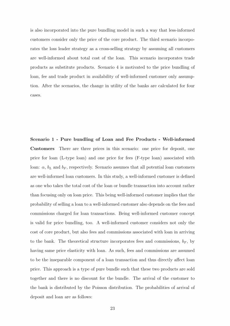
products as substitute products. Scenario 4 is motivated to the price bundling of

loan, fee and trade product in availability of well-informed customer only assump-

tion. After the scenarios, the change in utility of the banks are calculated for four

cases.

Scenario 1 - Pure bundling of Loan and Fee Products - Well-informed

Customers There are three prices in this scenario: one price for deposit, one

price for loan (L-type loan) and one price for fees (F-type loan) associated with

loan: α, bL and bF , respectively. Scenario assumes that all potential loan customers

are well-informed loan customers. In this study, a well-informed customer is defined

as one who takes the total cost of the loan or bundle transaction into account rather

than focusing only on loan price. This being well-informed customer implies that the

probability of selling a loan to a well-informed customer also depends on the fees and

commissions charged for loan transactions. Being well-informed customer concept

is valid for price bundling, too. A well-informed customer considers not only the

cost of core product, but also fees and commissions associated with loan in arriving

to the bank. The theoretical structure incorporates fees and commissions, bF , by

having same price elasticity with loan. As such, fees and commissions are assumed

to be the inseparable component of a loan transaction and thus directly affect loan

price. This approach is a type of pure bundle such that these two products are sold

together and there is no discount for the bundle. The arrival of the customer to

the bank is distributed by the Poisson distribution. The probabilities of arrival of

deposit and loan are as follows:

23

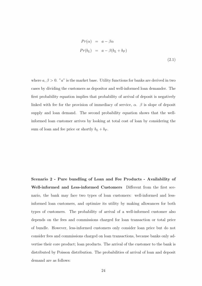
Pr(α) = a− βα

Pr(bL) = a− β(bL + bF )

(2.1)

where a, β > 0. ”a” is the market base. Utility functions for banks are derived in two

cases by dividing the customers as depositor and well-informed loan demander. The

first probability equation implies that probability of arrival of deposit is negatively

linked with fee for the provision of immediacy of service, α. β is slope of deposit

supply and loan demand. The second probability equation shows that the well-

informed loan customer arrives by looking at total cost of loan by considering the

sum of loan and fee price or shortly bL + bF .

Scenario 2 - Pure bundling of Loan and Fee Products - Availability of

Well-informed and Less-informed Customers Different from the first sce-

nario, the bank may face two types of loan customers: well-informed and less-

informed loan customers, and optimize its utility by making allowances for both

types of customers. The probability of arrival of a well-informed customer also

depends on the fees and commissions charged for loan transaction or total price

of bundle. However, less-informed customers only consider loan price but do not

consider fees and commissions charged on loan transactions, because banks only ad-

vertise their core product; loan products. The arrival of the customer to the bank is

distributed by Poisson distribution. The probabilities of arrival of loan and deposit

demand are as follows:

24

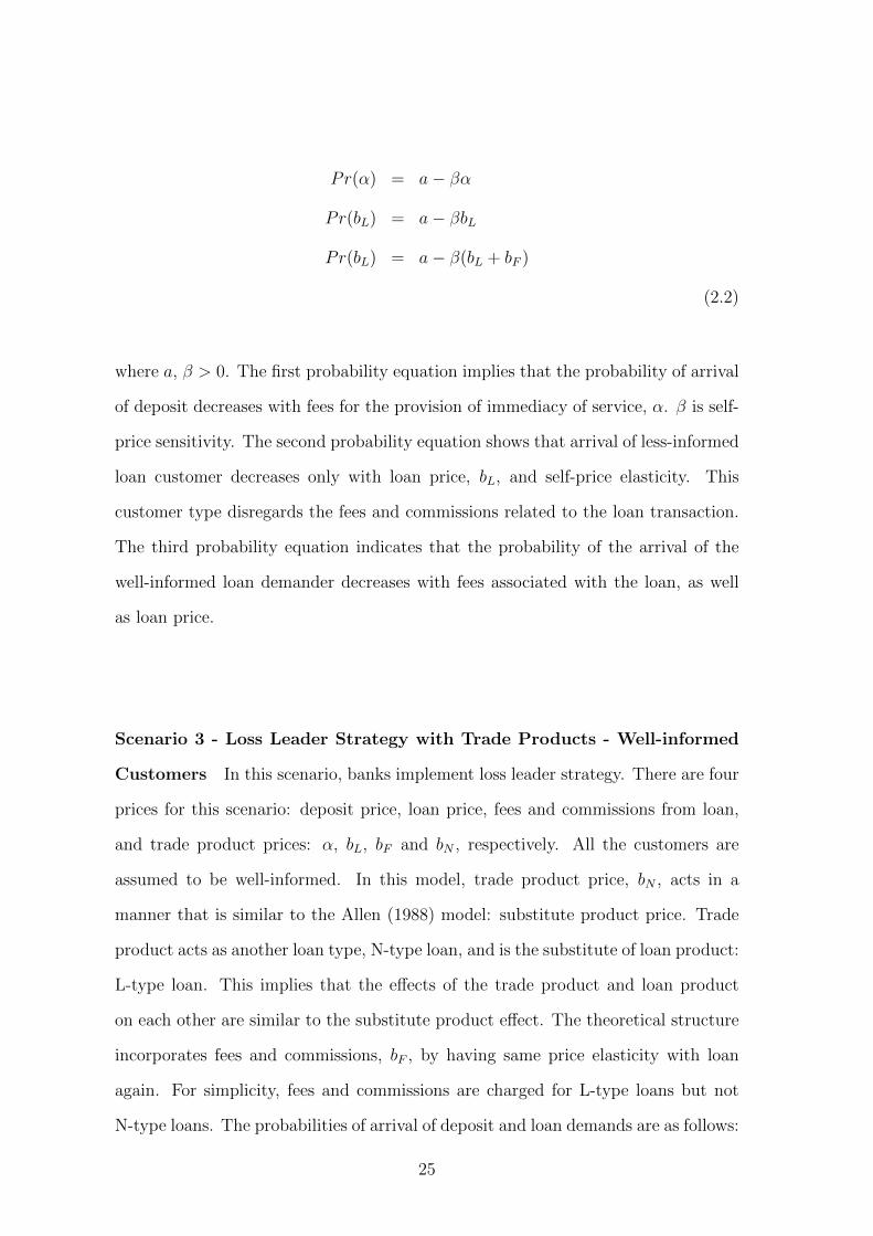
Pr(α) = a− βα

Pr(bL) = a− βbL

Pr(bL) = a− β(bL + bF )

(2.2)

where a, β > 0. The first probability equation implies that the probability of arrival

of deposit decreases with fees for the provision of immediacy of service, α. β is self-

price sensitivity. The second probability equation shows that arrival of less-informed

loan customer decreases only with loan price, bL, and self-price elasticity. This

customer type disregards the fees and commissions related to the loan transaction.

The third probability equation indicates that the probability of the arrival of the

well-informed loan demander decreases with fees associated with the loan, as well

as loan price.

Scenario 3 - Loss Leader Strategy with Trade Products - Well-informed

Customers In this scenario, banks implement loss leader strategy. There are four

prices for this scenario: deposit price, loan price, fees and commissions from loan,

and trade product prices: α, bL, bF and bN , respectively. All the customers are

assumed to be well-informed. In this model, trade product price, bN , acts in a

manner that is similar to the Allen (1988) model: substitute product price. Trade

product acts as another loan type, N-type loan, and is the substitute of loan product:

L-type loan. This implies that the effects of the trade product and loan product

on each other are similar to the substitute product effect. The theoretical structure

incorporates fees and commissions, bF , by having same price elasticity with loan

again. For simplicity, fees and commissions are charged for L-type loans but not

N-type loans. The probabilities of arrival of deposit and loan demands are as follows:

25

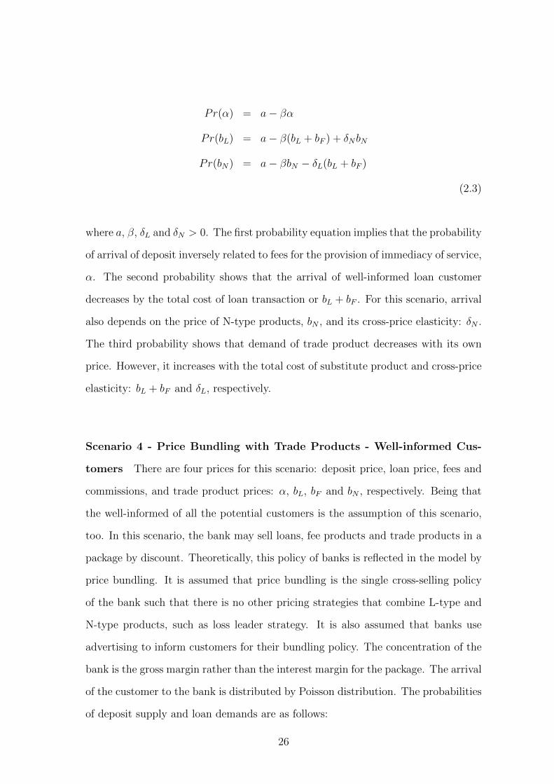
Pr(α) = a− βα

Pr(bL) = a− β(bL + bF ) + δNbN

Pr(bN) = a− βbN − δL(bL + bF )

(2.3)

where a, β, δL and δN > 0. The first probability equation implies that the probability

of arrival of deposit inversely related to fees for the provision of immediacy of service,

α. The second probability shows that the arrival of well-informed loan customer

decreases by the total cost of loan transaction or bL + bF . For this scenario, arrival

also depends on the price of N-type products, bN , and its cross-price elasticity: δN .

The third probability shows that demand of trade product decreases with its own

price. However, it increases with the total cost of substitute product and cross-price

elasticity: bL + bF and δL, respectively.

Scenario 4 - Price Bundling with Trade Products - Well-informed Cus-

tomers There are four prices for this scenario: deposit price, loan price, fees and

commissions, and trade product prices: α, bL, bF and bN , respectively. Being that

the well-informed of all the potential customers is the assumption of this scenario,

too. In this scenario, the bank may sell loans, fee products and trade products in a

package by discount. Theoretically, this policy of banks is reflected in the model by

price bundling. It is assumed that price bundling is the single cross-selling policy

of the bank such that there is no other pricing strategies that combine L-type and

N-type products, such as loss leader strategy. It is also assumed that banks use

advertising to inform customers for their bundling policy. The concentration of the

bank is the gross margin rather than the interest margin for the package. The arrival

of the customer to the bank is distributed by Poisson distribution. The probabilities

of deposit supply and loan demands are as follows:

26

Pr(α) = a− βα

Pr(bL) = a− β(bL + bF )

Pr(bN) = a− βbN

Pr(bL + bN) = a− β(bL + bF + bN + u)

(2.4)

where a, β > 0. Discount rate u is lower than 0 and is assumed to be exogenous.

The first probability equation implies that arrival of deposit decreases with fees for

the provision of immediacy of service, α. β is price elasticity of deposit supply and

loan demand. The second probability equation indicates that the probability of

arrival of well-informed loan demander decreases with loan price and fees associated

with loan. The third probability equation states that the demand of trade product

decreases with its own price. The fourth equation reveals the probability for demand

of price bundling. Bundle includes loan, fees and commissions, and trade products.

In case of simultaneous demand for loan and trade products, probability decreases

with increase in price of loan, bL, fees associated with loan, bF , and price of trade

product, bN , but increases with the discount factor, u.

Utilities for the Scenarios

For each different probability of arrival of customer, the bank has different utilities.

The total price information level of customers (well-informed or less-informed) does

not change the expected utility but changes the probability of arrival of customers

and therefore, it affects probability. Changes in the expected utilities are presented

in four cases: utility from arrival for deposit, L-type loan demand, N-type loan

demand and bundle demand. Change in the utilities are calculated as follows:

The initial wealth of the bank (W0) is determined by initial loans (L0), initial

deposits (D0) and initial net money market assets (M0), as in the Ho and Sounder’s

27

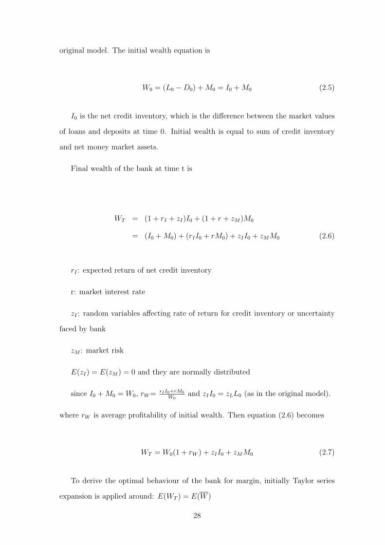
original model. The initial wealth equation is

W0 = (L0 −D0) +M0 = I0 +M0 (2.5)

I0 is the net credit inventory, which is the difference between the market values

of loans and deposits at time 0. Initial wealth is equal to sum of credit inventory

and net money market assets.

Final wealth of the bank at time t is

WT = (1 + rI + zI)I0 + (1 + r + zM)M0

= (I0 +M0) + (rII0 + rM0) + zII0 + zMM0 (2.6)

rI : expected return of net credit inventory

r: market interest rate

zI : random variables affecting rate of return for credit inventory or uncertainty

faced by bank

zM : market risk

E(zI) = E(zM) = 0 and they are normally distributed

since I0 +M0 = W0, rW= rII0+rM0

W0and zII0 = zLL0 (as in the original model).

where rW is average profitability of initial wealth. Then equation (2.6) becomes

WT = W0(1 + rW ) + zII0 + zMM0 (2.7)

To derive the optimal behaviour of the bank for margin, initially Taylor series

expansion is applied around: E(WT ) = E(W )

28

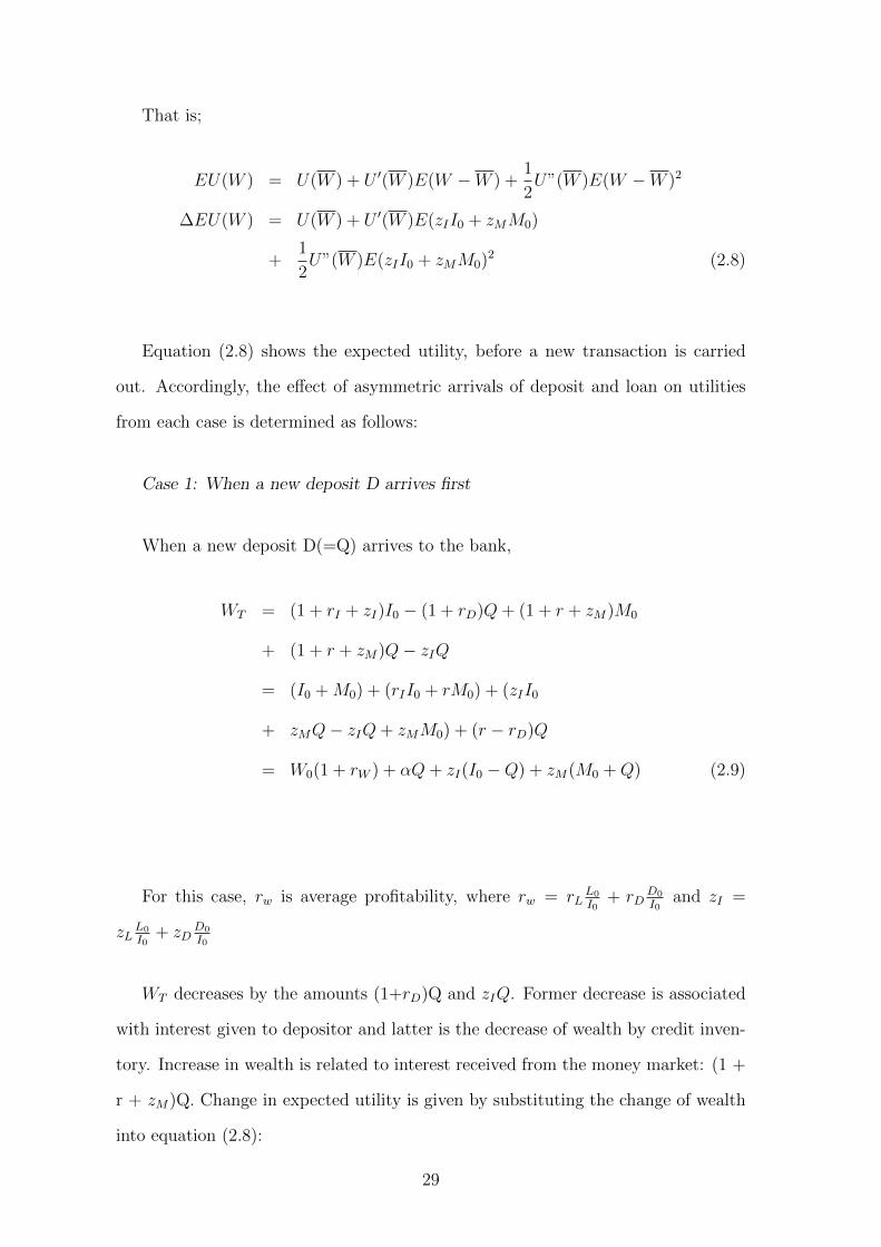
That is;

EU(W ) = U(W ) + U ′(W )E(W −W ) +1

2U”(W )E(W −W )2

∆EU(W ) = U(W ) + U ′(W )E(zII0 + zMM0)

+1

2U”(W )E(zII0 + zMM0)2 (2.8)

Equation (2.8) shows the expected utility, before a new transaction is carried

out. Accordingly, the effect of asymmetric arrivals of deposit and loan on utilities

from each case is determined as follows:

Case 1: When a new deposit D arrives first

When a new deposit D(=Q) arrives to the bank,

WT = (1 + rI + zI)I0 − (1 + rD)Q+ (1 + r + zM)M0

+ (1 + r + zM)Q− zIQ

= (I0 +M0) + (rII0 + rM0) + (zII0

+ zMQ− zIQ+ zMM0) + (r − rD)Q

= W0(1 + rW ) + αQ+ zI(I0 −Q) + zM(M0 +Q) (2.9)

For this case, rw is average profitability, where rw = rLL0

I0+ rD

D0

I0and zI =

zLL0

I0+ zD

D0

I0

WT decreases by the amounts (1+rD)Q and zIQ. Former decrease is associated

with interest given to depositor and latter is the decrease of wealth by credit inven-

tory. Increase in wealth is related to interest received from the money market: (1 +

r + zM)Q. Change in expected utility is given by substituting the change of wealth

into equation (2.8):

29

∆EU(W |D) = U ′(W )αQ+1

2U”(W )[(αQ)2

+ (Q− 2I0)Qσ2I + (Q+ 2M0)Qσ2

M

+ 2(I0 −M0 −Q)QσIM ]

= U ′(W )αQ+1

2U”(W )[(αQ)2 + PQ] (2.10)

where

P = (Q− 2I0)σ2I + (Q+ 2M0)σ2

M + 2 (I0 −M0 −Q)σIM

Case 2 - Request for L-type loan

When a new loan L(=Q) transaction is made rather than a deposit,

WT = W0(1 + rW ) + (bL + bF )Q+ zI(I0 + 2Q) + zM(M0 − 2Q)

(2.11)

where

rw = rLL0

I0+ rF

F0

I0+ rD

D0

I0and zI = zL

L0

I0+ zF

F0

I0+ zD

D0

I0

Increase in wealth is associated with the sum of the loan and fee prices charged

on the loan: bL + bF . Change in wealth also depends on zMQ and zIQ, which

reflect the change in wealth from the money market position and credit inventory,

respectively. Then,

∆EU(W |L) = U ′(W )(bL + bF )Q+1

2U”(W )[((bL + bF )Q)2 +GQ] (2.12)

where

G = (4Q+ 4I0)σ2I + (4Q− 4M0)σ2

M + 2(2M0 − 2I0 − 4Q)σIM

30

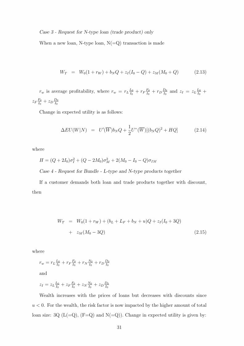
Case 3 - Request for N-type loan (trade product) only

When a new loan, N-type loan, N(=Q) transaction is made

WT = W0(1 + rW ) + bNQ+ zI(I0 −Q) + zM(M0 +Q) (2.13)

rw is average profitability, where rw = rLL0

I0+ rF

F0

I0+ rD

D0

I0and zI = zL

L0

I0+

zFF0

I0+ zD

D0

I0

Change in expected utility is as follows:

∆EU(W |N) = U ′(W )bNQ+1

2U”(W )[(bNQ)2 +HQ] (2.14)

where

H = (Q+ 2I0)σ2I + (Q− 2M0)σ2

M + 2(M0 − I0 −Q)σIM

Case 4 - Request for Bundle - L-type and N-type products together

If a customer demands both loan and trade products together with discount,

then

WT = W0(1 + rW ) + (bL + LF + bN + u)Q+ zI(I0 + 3Q)

+ zM(M0 − 3Q) (2.15)

where

rw = rLL0

I0+ rF

F0

I0+ rN

N0

I0+ rD

D0

I0

and

zI = zLL0

I0+ zF

F0

I0+ zN

N0

I0+ zD

D0

I0

Wealth increases with the prices of loans but decreases with discounts since

u < 0. For the wealth, the risk factor is now impacted by the higher amount of total

loan size: 3Q (L(=Q), (F=Q) and N(=Q)). Change in expected utility is given by:

31

∆EU(W |L+N) = U ′(W )(bL + bF + bN + u)Q

+1

2U”(W )[((bL + bF + bN + u)Q)2 + JQ] (2.16)

where

J = (9Q+ 6I0)σ2I + (9Q− 6M0)σ2

M + 2(3M0 − 3I0 − 9Q)σIM

2.3.2 Maximizations

Maximization in Scenario 1

Proposition 1 In pure bundling of loan and, fees and commissions, in the presence

of well-informed customers, the effect of fees and commissions on net interest margin

will be negative and reduce it by its own value.

Scenario 1 presents the probabilities in case of three products: deposit, loan and

fee products in the assumption of well-informed customers. To derive the optimal

values of α, bL and bF , probabilities in scenario 1 are multiplied by change in expected

utility for each probability. Then, optimization is made with respect to α, bL and

bF .

The maximization problem is as follows:

∆EU(W ) = (a− βα)∆EU(W |D) + (a− β(bL + bF ))∆EU(W |L) (2.17)

First, the derivative of equation (2.17) with respect to α is2

∂∆EU(W )

∂α= −β[U ′(W )αQ+

1

2U”(W )PQ] + (a− βα)U ′(W )Q (2.18)

Then, by rearranging, we derive optimal α

2the second-order terms of the margins and costs of the Taylor’s expansion are negligible dueto efficient portfolio assumption.

32

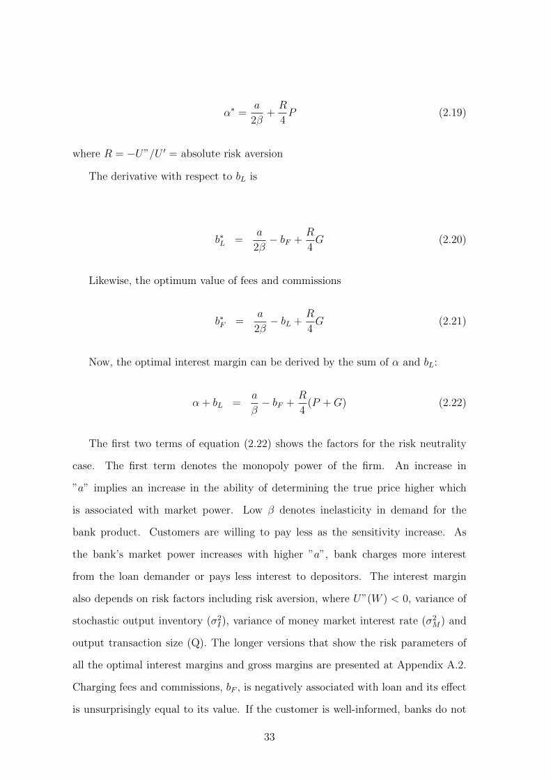
α∗ =a

2β+R

4P (2.19)

where R = −U”/U ′ = absolute risk aversion

The derivative with respect to bL is

b∗L =a

2β− bF +

R

4G (2.20)

Likewise, the optimum value of fees and commissions

b∗F =a

2β− bL +

R

4G (2.21)

Now, the optimal interest margin can be derived by the sum of α and bL:

α + bL =a

β− bF +

R

4(P +G) (2.22)

The first two terms of equation (2.22) shows the factors for the risk neutrality

case. The first term denotes the monopoly power of the firm. An increase in

”a” implies an increase in the ability of determining the true price higher which

is associated with market power. Low β denotes inelasticity in demand for the

bank product. Customers are willing to pay less as the sensitivity increase. As

the bank’s market power increases with higher ”a”, bank charges more interest

from the loan demander or pays less interest to depositors. The interest margin

also depends on risk factors including risk aversion, where U”(W ) < 0, variance of

stochastic output inventory (σ2I ), variance of money market interest rate (σ2

M) and

output transaction size (Q). The longer versions that show the risk parameters of

all the optimal interest margins and gross margins are presented at Appendix A.2.

Charging fees and commissions, bF , is negatively associated with loan and its effect

is unsurprisingly equal to its value. If the customer is well-informed, banks do not

33

obtain extra profit from advertising the core product only. On the other hand, gross

margin, as the main focus of the bank, will be

α + bL + bF =3a

2β− (bL + bF ) +

R

4(P + 2G) (2.23)

Maximization in Scenario 2

Proposition 2 In being of less-informed loan customers, a bank can get higher gross

margins by pure bundling of loan and fee income, when bF4> bL

2

In scenario 2, the bank considers both well-informed and less-informed customers

for their loan product. The maximization problem takes the form:

∆EU(W ) = (a− βα)∆EU(W |D)

+ (a− βbL)∆EU(W |L)

+ (a− β(bL + bF ))∆EU(W |L) (2.24)

First, the derivative of equation (2.24) with respect to α is

∂EU(W )

∂α= −β[U ′(W )αQ+

1

2U”(W )PQ] + (a− βα)U ′(W )Q

(2.25)

Then, optimal α is

α∗ =a

2β+R

4P (2.26)

The derivative with respect to bL is

b∗L =a

2β− 3

4bF +

R

4G (2.27)

34

The optimum value of fees and commissions is derived by taking derivative with

respect to bF .

b∗F =a

2β− 3

2bL +

R

4G (2.28)

The optimal interest margin for scenario 2 is:

α∗ + b∗L =a

β− 3

4bF +

R

4(P +G) (2.29)

First term in equation (2.29) denotes the monopoly power of the firm. There is

no differences between first and second scenario in terms of market power. Absolute

risk aversion affects the margin by the same magnitude with first scenario. Charging

fees and commissions, bF , from loan is negatively associated with loan price and its

effect is no longer equal to its value. Gross margin, as the main focus of the bank,

will be

α∗ + b∗L + b∗F =3a

2β− 3

2(bL −

bF2

) +R

4(P + 2G) (2.30)

The difference between equation (2.30) and equation (2.23) gives the differences

for gross margin with well-informed customers only and availability of both well-

informed and less-informed customers:

Eq(2.30)− Eq(2.23) =bF4− bL

2(2.31)

The equation above states that in the availability of both well-informed and less-

informed customers, bank can increase their gross margin by lowering loan price and

increasing fees and commissions.

35

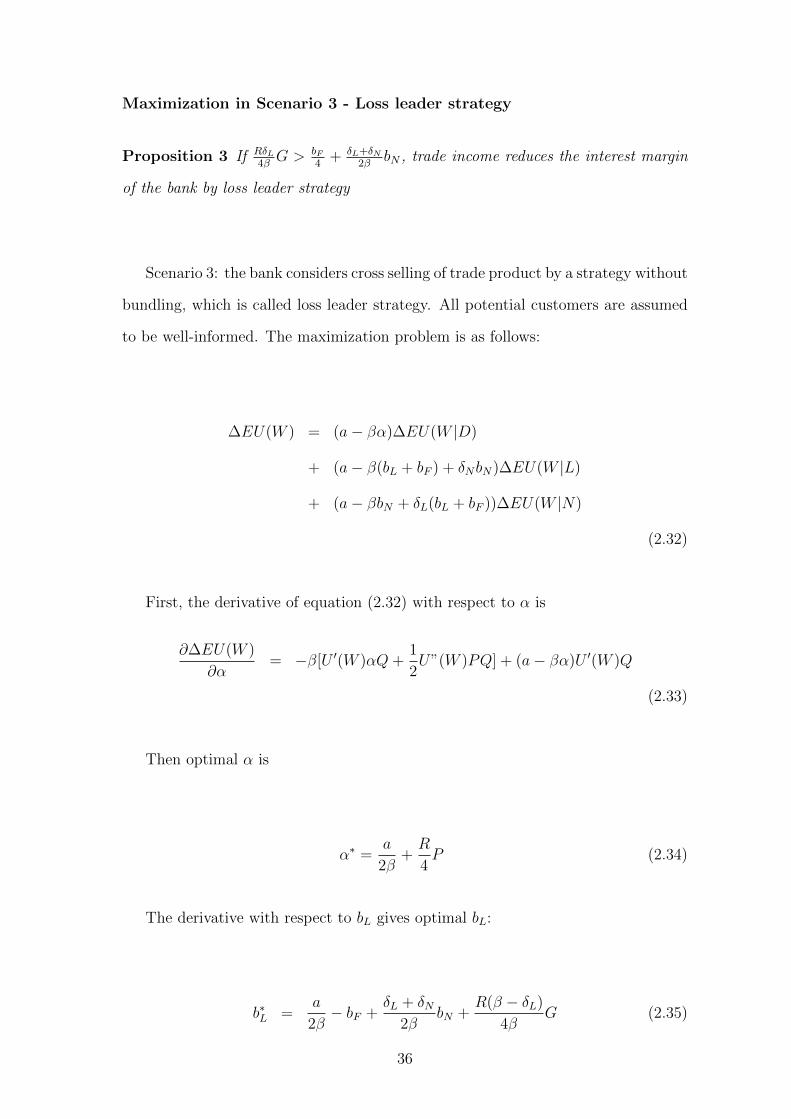
Maximization in Scenario 3 - Loss leader strategy

Proposition 3 If RδL4βG > bF

4+ δL+δN

2βbN , trade income reduces the interest margin

of the bank by loss leader strategy

Scenario 3: the bank considers cross selling of trade product by a strategy without

bundling, which is called loss leader strategy. All potential customers are assumed

to be well-informed. The maximization problem is as follows:

∆EU(W ) = (a− βα)∆EU(W |D)

+ (a− β(bL + bF ) + δNbN)∆EU(W |L)

+ (a− βbN + δL(bL + bF ))∆EU(W |N)

(2.32)

First, the derivative of equation (2.32) with respect to α is

∂∆EU(W )

∂α= −β[U ′(W )αQ+

1

2U”(W )PQ] + (a− βα)U ′(W )Q

(2.33)

Then optimal α is

α∗ =a

2β+R

4P (2.34)

The derivative with respect to bL gives optimal bL:

b∗L =a

2β− bF +

δL + δN2β

bN +R(β − δL)

4βG (2.35)

36

The optimum value of fees and commissions

b∗F =a

2β− bL +

δL + δN2β

bN +R(β − δL)

4βG (2.36)

The optimal value of trade product is

b∗N =a

2β+δL + δN

2β(bL + bF ) +

R(β − δL)

4βH (2.37)

The optimal interest margin for scenario 3 is:

α∗ + b∗L =a

β− bF +

δL + δN2β

bN +R

4P +

R(β − δL)

4βG (2.38)

Charging fees and commissions, bF , is negatively associated with loan and its

effect is equal to its value as in scenario 1 due to the customers’ being well-informed.

For this scenario, interest margin is also determined by cross-price elasticity of N-

type product, δN , and cross-price elasticity of L-type product, δL. Increase in the

cross-price elasticity of N-type product (trade product), increases the interest margin

of the bank. Interest margin without the trade product is known from the base

scenario. If interest margin of the scenario 3 is lower than the interest margin of

scenario 1, then the impact of trade income will be negative:

Eq(2.38)− Eq(2.22) =bF4

+δL + δN

2βbN −

RδL4β

G (2.39)

if δL4βRG > bF

4+ δL+δN

2βbN , trade income reduces the interest margin of the bank.

The optimal gross margin is

37

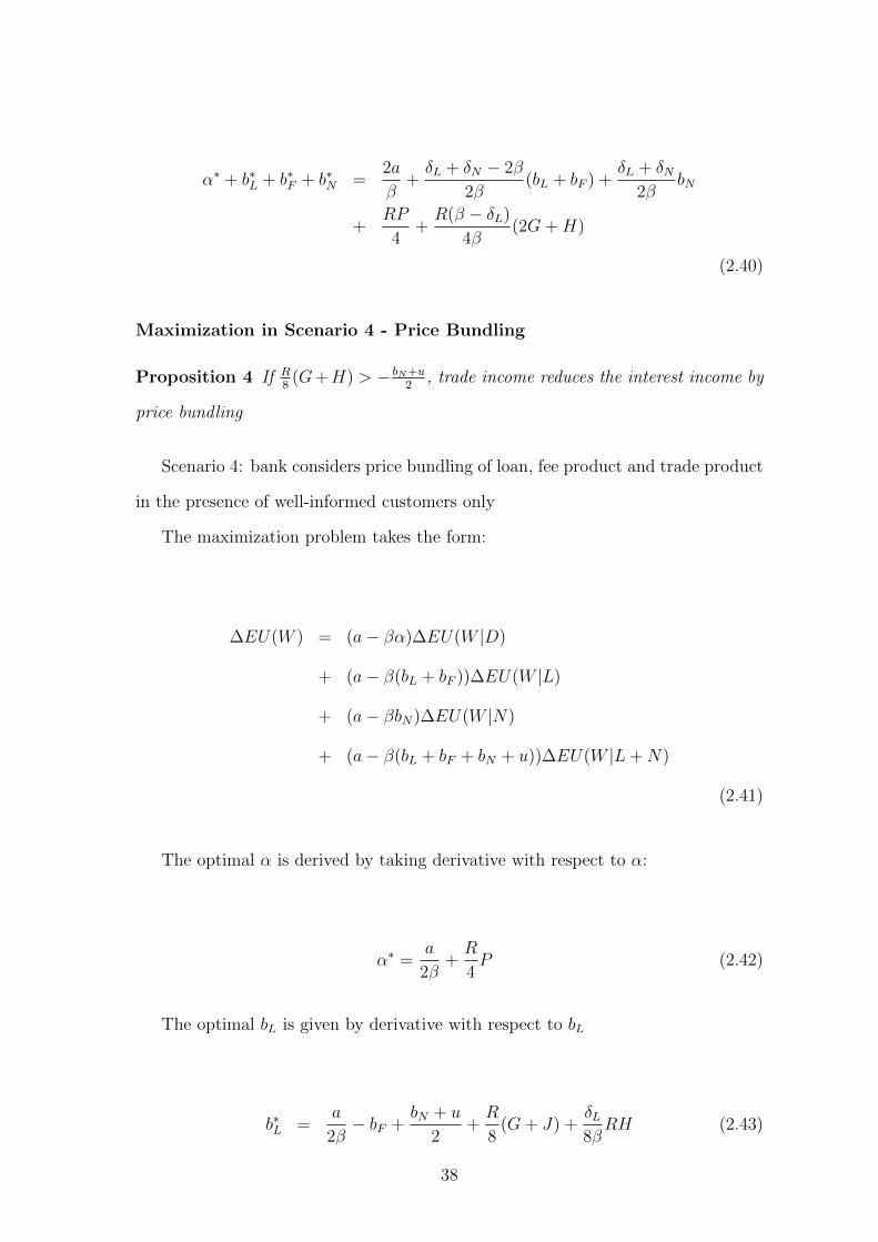
α∗ + b∗L + b∗F + b∗N =2a

β+δL + δN − 2β

2β(bL + bF ) +

δL + δN2β

bN

+RP

4+R(β − δL)

4β(2G+H)

(2.40)

Maximization in Scenario 4 - Price Bundling

Proposition 4 If R8

(G+H) > − bN+u2

, trade income reduces the interest income by

price bundling

Scenario 4: bank considers price bundling of loan, fee product and trade product

in the presence of well-informed customers only

The maximization problem takes the form:

∆EU(W ) = (a− βα)∆EU(W |D)

+ (a− β(bL + bF ))∆EU(W |L)

+ (a− βbN)∆EU(W |N)

+ (a− β(bL + bF + bN + u))∆EU(W |L+N)

(2.41)

The optimal α is derived by taking derivative with respect to α:

α∗ =a

2β+R

4P (2.42)

The optimal bL is given by derivative with respect to bL

b∗L =a

2β− bF +

bN + u

2+R

8(G+ J) +

δL8βRH (2.43)

38

Similarly, the optimum value of fees and commissions is equal to value of bL by

replacement of bF with bL

b∗F =a

2β− bL +

bN + u

2+R

8(G+ J) +

δL8βRH (2.44)

The optimal value of trade product is

b∗N =a

2β− bL + bF + u

2+R

8(G+ J) +

δN8βRH (2.45)

The optimal interest margin for scenario 4 is given by:

α∗ + b∗L =a

β− bF −

bN + u

2+R

8(2P +G+ J) +

δL8βRH

(2.46)

If interest margin of the scenario 4 is lower than interest margin of scenario 1,

then the impact of trade income to the interest margin will be negative:

Eq(2.46)− Eq(2.22) = −bN + u

2− R

8(G+H) (2.47)

if R8

(G+H) > − bN+u2

, trade income reduces the interest income in price bundling

case.

Gross margin, as the main focus of the bank, will be

α∗ + b∗L + b∗F + b∗N =2a

β− 3

2(bL + bF − u)− bN +

R

4(P +G+ J)

+R(2δL + δN)

8βH

(2.48)

In summary, scenario 1 states that pure bundling of fees and commissions re-

39

duces the interest margin in the assumption of all customers’ being well-informed.

According to scenario 2, banks can increase their gross margin by lowering the price

of their loan product and compensating it by fees and commissions in the avail-

ability of less-informed customers. Scenarios 3 and 4 show the effect of loss leader

and price bundling strategies, respectively. By using convenient strategies, banks

may create a relationship between loan and non-interest products, including trade

products. Trade income reduces the interest margin if the conditions given above

are satisfied.

The theoretical contribution of this thesis is mainly associated with strategies in

cross-selling by considering bundling strategies and differentiating non- interest in-

come components. First, the original model of Ho and Saunders doesn’t consider the

effect of non-interest income on net interest margin. carbo˙valverde˙determinants˙2007

incorporated the effect of the non-interest income on interest margin in the multi-

output framework. Their study includes the effect of fees in the presence of loss-

leader strategy. However, this thesis creates this relationship by considering the very

popular strategy: bundling. Second, the study also differentiates bundling strate-

gies, including pure and price bundling. Particularly price bundling contributes to

the literature by distinguishing between fees and commission income and trade in-

come. Incorporating trade income to the model, rather than considering fees and

commissions only, this study reveals the bank strategy such that banks do not only

try to charge some fees and commissions from loan activity, but also struggle to

sell some complement or other independent products to the core customers, like

insurance. Third, original model and other extensions have no assumptions on the

information level of the customers. Banks benefit from the information level differ-

ences of the customers about the total cost of the loan by advertising the price of

loan product only and charge fees and commissions from the lending activity. This

study reveals this strategy by differentiating the customers as less-informed and

well-informed and shows that compared to the assumption of all customers’ being

well-informed, banks can improve their gross margin in the presence of less-informed

40

customers.

2.4 Data

Yearly banking data are collected from the Bureau Van Disk’s Bankscope Database.

Macroeconomic details are obtained from the World Bank’s World Development In-

dicators (WDI). Unconsolidated commercial and saving bank financial data is used

but in the absence of unconsolidated data, banks’ consolidated data were added to

the data pool. The data is from 2004 to 2011. All bank data values are dollar

values and were deflated by the gross domestic product deflator. The ratios were

multiplied by 1000 to see the std errors more clearly. The sample consists of twelve

European countries including Austria, Belgium, Switzerland, Czech Republic, Den-

mark, Finland, France, United Kingdom, Netherlands, Sweden, Turkey and Norway.

From the 1970s and 1980s onwards, commercial banks in these countries have been

allowed to engage in a wide range of financial services and, therefore, to diversify

their output to a larger extent. Despite dramatic progress in banking regulations

in Turkey particularly in the 2000’s, potential regulatory differences in Turkey is

considered, and results show that there is no any change in significance of variables

by removing/adding Turkey. The current sample thus also represents the European

OECD countries. All of these European countries are OECD members, too. There

are still regulatory and institutional differences across some countries, which makes

a ’country by country’ analysis advisable as a robustness check. The sample contains

a total of 896 banks.

The sample used in this analysis is less than the actual total number of obser-

vations, but it considered the representativeness of sample. Some of the criteria

reduces the number of observations. The criteria implemented in filtering are:

i Missing years from explanatory variables and independent variable were elim-

inated

ii Observations contradicting with their nature were also eliminated. For ex-

41

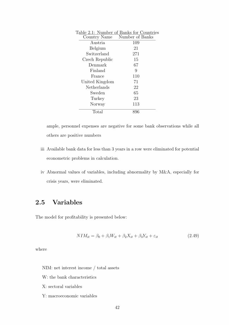
Table 2.1: Number of Banks for CountriesCountry Name Number of Banks

Austria 109Belgium 21

Switzerland 271Czech Republic 15

Denmark 67Finland 9France 110

United Kingdom 71Netherlands 22

Sweden 65Turkey 23Norway 113

Total 896

ample, personnel expenses are negative for some bank observations while all

others are positive numbers

iii Available bank data for less than 3 years in a row were eliminated for potential

econometric problems in calculation.

iv Abnormal values of variables, including abnormality by M&A, especially for

crisis years, were eliminated.

2.5 Variables

The model for profitability is presented below:

NIMit = β0 + β1Wit + β2Xit + β3Yit + εit (2.49)

where

NIM: net interest income / total assets

W: the bank characteristics

X: sectoral variables

Y: macroeconomic variables

42

ε: the error term

2.5.1 Dependent Variable

Net Interest Margin (NIM) : bank interest margin can be interpreted as an

indicator of the bank profitability. It is calculated as the quotient between net inter-

est income and total asset, like in Demirguc-Kunt and Huizinga (1999) and, Maudos

and Guevara (2004). Ho and Saunders (1981) and Lepetit et al. (2008b) compute net

interest margin as interest income minus interest expense divided by earning assets.

Alternatively, Lepetit et al. (2008b) also calculate the dependent variable as the

difference between interest from loans over net loans and interest expenses divided

by total liabilities. Angbazo (1997) defines net interest margin as the difference

between interest revenues over earning assets and interest cost (quotient between

interest expenses minus loan loss provisions and interest bearing liabilities). Carbo

and Fernandez (2007) calculates the profitability as loan to deposit rate which is

the difference between interest income divided by loans and interest expense over

deposits.

One of the alternative measurements of profitability is the net interest income

over equity ratio as ROE. The difference between the return on asset and return

on equity is the effect of share of debt and equity. Risk-averse banks may prefer

to hold more equity rather than debt and take less risk. Therefore, higher return

on equity is not always a good indicator to measure bank profitability performance,

but it is still important measurement in regarding total risk/return trade-off. In this

context, this study prefers to use ROA rather than ROE, because the main objective

of the second chapter is not the risk/return measurement even effect of the risk is

an important factor in the regression models in this chapter.

43

2.5.2 Explanatory Variables:

Bank Characteristics:

Market Power (LERNER) : the market structure and the effect of market

power on net interest margin is measured by using Lerner index in this analysis.

Lerner index is widely used as a direct measure of market power in the banking

sector. The market power concept is appropriate if market includes the oligopoly

case and the banking sector is a good sector to use market power measurement

in terms of oligopoly. Maudos and Guevara (2004) and, Maudos and Solis (2009)

calculate market power by using Lerner index in explaining net interest margin.

Li =Pi −MCi

Pi(2.50)

where

Li= Lerner index

Pi= Total revenue of bank: Total revenue from interest and non-interest activi-

ties. Here, total revenue measures the bank price

MCi = Marginal cost of producing an additional unit of product. Marginal cost

is the derivative of the total cost function with respect to the output (Q).

Translogarithmic total cost equation takes the form:

lnTC = β0 + b0lnTA+1

2b1lnTA

2 +3∑j=1

βi ∗ lnwji

+1

2b2lnTAlnw1 +

1

2b3lnTAlnw2 +

1

2b4lnTAlnw3

+3∑j=1

3∑k=1

βjklnwji + Trend+ Trend2 (2.51)

where

TC: total cost (total financial and operational cost)

TA: total asset

w1: (total cost - personnel cost)/ total assets

44

w2: personnel cost/ fixed assets

w3: total interest expense / short term funding

Trend: trend term

The Lerner index formula measures a relative mark-up price over marginal cost.

Market power in here is the ability of keeping prices higher relative to marginal cost.

One homogeneity is constrained in this translogarithmic function.

Marginal cost is derived by taking the derivative of the total cost equation with

respect to Q (in here TA).

MC = b0 +1

2b1lnTA+

1

2

3∑i=1

bilnwi (2.52)

Personnel Expenses (PERSONNEL) : Calculated as personnel expenses to

total asset ratio. The alternative to personnel expenses is the operating expense.

The literature presents mixed results on operating expenses. Banks with higher oper-

ating expenses may add operating costs to their interest margin. Whereas, increases

in operating costs may end with stronger provision by increasing the screening and

monitoring of borrowers. Therefore, mainly, personnel expenses variable (PERSON-

NEL) is tested rather than operational costs (OPERCOST), as operational costs of

the bank over total asset ratio, but OPERCOST is also tested for robustness check.

Bank’s Risk Aversion (EQUITY) : The quotient between equity and total as-

set is introduced to measure a bank’s risk aversion similar to McShane and Sharpe

(1985), Angbazo (1997), Drakos (2002), Maudos and Guevara (2004) and Le Lepetit

et al. (2008b). Higher capital to asset ratio reduces a bank’s deposit funding and

provides a disincentive for taking more risk. From the standard capital structure

theory perspective, holding more capital alleviates the cost of funding thus enhanc-

ing interest rates. In contrast, Admati et al. (2013) suggest that higher capital

requirement reduces the risk premia in bank’s cost of funding.

45

Table 2.2: Descriptive Statistics - 1

Year Banks Statistics NIM Lerner Fees Cash Equity Trade TNII Efficiency

2004 626 Mean .0224 .2058 .0116 .0193 .0898 1.0151 -.0101 .4482

2004 626 Std Dev .0132 .2192 .0246 .0376 .0790 14.2457 .0160 .2357

2005 754 Mean .0213 .2190 .0117 .0185 .0888 2.3132 -.0084 .4253

2005 754 Std Dev .0124 .1980 .0293 .0300 .0756 10.977 .0163 .2253

2006 807 Mean .0204 .2222 .0124 .0200 .0903 1.3346 -.0070 .3879

2006 807 Std Dev .0122 .1040 .0321 .0439 .0763 10.3667 .0159 .1438

2007 825 Mean .0204 .1967 .0112 .0208 .0886 1.6414 -.0076 .3482

2007 825 Std Dev .0119 .0954 .0253 .0434 .0740 7.5459 .0146 .1302

2008 869 Mean .0208 .1345 .0103 .0263 .0871 1.6487 -.0115 .3541

2008 869 Std Dev .0118 .3828 .0232 .0422 .0724 7.0435 .0166 .2258

2009 788 Mean .0199 .1828 .0093 .0282 .0904 1.1174 -.0091 .4572

2009 788 Std Dev .0140 .3235 .0152 .0536 .0828 6.8633 .0118 .3318

2010 886 Mean .0186 .1820 .0097 .0294 .0931 1.7789 -.0090 .4776

2010 886 Std Dev .0116 .3330 .0218 .0575 .0826 8.9901 .0120 .3305

2011 876 Mean .0188 .1711 .0086 .0346 .0919 .8454 -.0099 .4646

2011 876 Std Dev .0118 .2774 .0159 .0638 .0840 9.7324 .0172 .2875

NIM: net interest income/total assets, LERNER: lerner index, FEES: net fees and commissions over net non-interest in-

come, CASH: cash and due from banks/total Assets, EQUITY: equity/total assets, TRADE: net non-interest income mi-

nus net fees and commissions over total assets, TNII: net non-interest income over total assets, EFFICIENCY: operating

cost to gross income

46

Liquidity Risk (CASH) : Liquidity is measured by cash and due from banks to

total asset ratio. An increase in liquidity may reduce the bank’s liquidity risk, which

alleviates the interest margin due to a lower liquidity premium charged on loans. A

positive relationship, which implies increase in interest margin with risk aversion, is

expected.

Average Size of Loans (SIZE) : In this extended version of bank dealership

model, loan size (Q) is negatively associated with margin. Unfortunately, Bankscope

data and annual reports of banks are insufficient to calculate the average size of the

bank loan. To measure average size, the logarithm of loan is used as a proxy for

loan size.

Fees and Commissions (FEES) : Banks determine their loan rates by consid-

ering fees and commissions to offset the loss from one part by increasing the price

of the other side. Generally, banks add fees and commissions costs as insepara-

ble components of loan transaction by bundling. Or, sometimes, banks underprice

their loan to sell complement of loans as fee product. Therefore, it is reasonable to

expect a negative relationship between fees and commissions, and interest margin.

The effect of fees and commissions is measured by net fees and commissions to net

non-interest operating income ratio.

Future Fees and Commissions (FEESNP) : To test the potential loss leader

strategy of banks for the longer period effect, future fees and commissions income

is also tested. FEESNP is the time t+1 value of FEES variable.

Trade Income (TRADE) : TRADE is the quotient between net non-interest

income minus net fees and commissions over total assets. Lepetit et al. (2008b) and,

Maudos and Solis (2009) find a negative but insignificant relationship between trade

income and interest margin. However, very recent data is used in this analysis and

the relationship between trade products with loans may change due to new pricing

strategies or technology, during the newer period. On the other hand, the Bankscope

47

database differentiates insurance income and fess and commissions. Implementing

same formula used in the literature for the trade products but considering the com-

plementary feature of insurance income, this study expect a negative relationship

with interest margin.

Future Trade Income (TRADENP) : To understand the bank strategy more

appropriately, loss leader strategy for trade and interest products is also introduced

for longer periods. Banks generally advertise their core product and compensate it

with a non-traditional product. Banks feel confident charging fees from loan activi-

ties. However, there is no guarantee of this strategy for trade products. Therefore,

the potential significant relationship between interest and trade income requires

more detailed analysis to understand pricing strategy. Future period relationship

enhances the probability of loss leader strategy, but insignificance of relationship

between time t+1 values of trade income with time t interest income questions the

loss leader strategy, while time t relationship is significant. Bundling strategy only

implies same period relationship but loss leader strategy generally implies differ-

ent period relationship. In this vein, different period trade income variables are

also tested to find clues about price mechanisms. TRADENP, time t+1 value of

TRADE, measures the effect of trade income at time t+1.

Efficiency (EFFICIENCY) : Efficiency is proxied by the cost to income ratio

which is defined as the operating cost to produce gross income. Gross income is the

sum of gross interest and dividend income, and total non-interest operating income.

Sector Variables

Development of Sector (ASSETSGDP) : The effect of the banking sector

development is measured by total banking sector assets over GDP ratio. Total

banking sector assets are calculated for each country. Growth of the sector increases

the supply of funds and alleviates the margin.

48

Macroeconomic Variables

GDP Growth Rate (GDPGROWTH) : Higher GDP growth contributes to

capital accumulation and may, hence, increase the amount of funds. Increasing the

GDP growth of a country also attracts foreign capitals. These two factors enhance

the supply of funds. Improvements in funding conditions are expected to reduce

margins.

Inflation (INFLATION) : Higher inflation implies uncertainty in the economy

and banking sector. In the higher inflation period, it is difficult to determine ex-ante

interest rates. In this uncertainty, banks are willing to charge higher interest rates.

This study also uses time dummies to capture the specific effects of each year.

Furthermore, because the sample includes twelve European countries, country-specific

differences are captured by using country dummies in the models.

2.6 Methodology for Empirical Study

The classical ordinary least square regression model takes the form of

yi,t = βxi,t + εi,t (2.53)

where yi,t is the dependent variable and xi,t denotes the set of explanatory variables.

εi,t is the error term at time t. OLS methodology gives unbiased results if there is no

any unobserved heterogeneity in the error term. Otherwise estimates will become

biased. The bias of an estimator is the difference between the estimator’s expected

value and the true value of the parameter. However, in the presence of unobserved

heterogeneity, unobserved effects panel model will be

yi,t = βxi,t + αi + εi,t (2.54)

49

where αi is the time invariant unobserved heterogeneity in the error term. For these

models, fixed effect method requires that a strict exogeneity assumption must be

satisfied for the consistency of the estimators. Consistent estimator is an estimator

having the feature that as the sample size increases, the estimates converge to the

true value of the parameter being estimated. Therefore the condition below must

be satisfied for consistency

E(εi,t|αi, xi) = 0 (2.55)

Suppose that model requires dynamicity such that one of the explanatory variable

is the lag value of the dependent variable. In this case our model will be

yi,t = ϕyi,t−1 + βxi,t + αi + εi,t (2.56)

In this case, fixed effect model can’t be used to estimate the model, because yi,t

is correlated with the past values of error term, εi,t−1, and this is the violation of

strict exogeneity of the parameters (Roodman, 2006). Also, the weaker condition of

zero contemporaneous correlation of the regressors with the composite error term,

αi+εi,t, is violated, because there is a serial correlation in the composite error term.

Time invariant unobserved effect, αi, is the source of the serial correlation.

To solve the endogeneity problem and obtain consistent estimators, instrumental

variable (IV) technique is used. Instrumental variable is the variable that correlated

with explanatory variable being estimated and uncorrelated with the error term.

However, unobserved heterogeneity is still problem despite solving the endogeneity

problem above by instrumental variables. Unobserved effect, αi, is correlated with

lagged dependent variable. To settle the problem, Arellano and Bond (1991) pro-

pose the first difference to eliminate this bank-specific effect. After taking the first

difference, the model is given by

50

∆yi,t = ϕ∆yi,t−1 + β′∆xi,t + ∆εi,t (2.57)

Here, the error term εi,t − εi,t−1 is correlated with yi,t − yi,t−1. In this sense GMM

methodologies, as linear and dynamic methodologies, are introduced to remove

this correlation. GMM is an estimation method that has a objective function in

a quadratic form:

minM(β)′WM(β) (2.58)

where M(β) is a column vector of empirical moment conditions so that required

minimization is determined by the parameter β.

One of the alternatives to the taking first difference is the using forward orthog-

onal deviations, suggested by Arellano and Bover (1995). The forward orthogonal

deviation is implemented where the average of future values of each variable are

deducted from the current value. This methodology helpful in the availability of

missing variables and it also protects the degree of freedom.

In the differenced GMM, the past values of dependent variable are used as the

instruments for the current first differences of the dependent variable. The problem

in first difference GMM is the weak instrument. There are two cases that create a

less informative GMM estimation in the standard first differenced GMM. Variance

of the firm specific effect increases relative to the transitory shocks. Secondly, as

the coefficient of the lagged dependent variable approaches the unity, which means

ϕ approaches to the 1, GMM may become a weak instrument. In this vein, Blundell

and Bond (1998) show that weak instruments create a large finite sample bias in the

estimation of the autoregressive model. Another dynamic method, System GMM,

introduces an additional assumption which generates additional instruments. The

additional assumption is

51

E(∆yi,t−s[αi + εi,t]) = 0 (2.59)

This assumption requires that lagged differences in the dependent variable are

valid instruments for the level of the lagged dependent variable in the level equation.

If this assumption is true, then by the increase in the number of instruments, the

greater efficiency is achieved. Efficiency is the term associated with lower variance.

Lower variance means individual data are those that are closer to the mean value.

This implies that distributions of the estimates become more concentrated around

the true value of parameter being estimated and therefore the probability of true

estimation will increase. Unlike to differenced GMM, System GMM also estimate

the time invariant regressors by using the level equation of the dynamic model.

System GMM also assumes that there will be no correlation of the unobserved

effects and error terms across cross-section units. However, one of the difficulties

of the System GMM is the over-identification problem. If the number of moment

conditions is higher than the dimension of the parameter vector, the model is said

to be over-identified. Identification issue allows us to test whether the model’s

moment conditions match the data properly or not. In this vein, Hansen test is

used to detect over-identification is available or not under the null hypothesis that

all of the instruments are valid.

Lastly, the degree of serial correlation in ε will determine the validity of instru-

ments. By construction, the residuals of differenced equation should include serial

correlation, but serial independence is assumed in the original errors. We can test

serial correlations under the null hypothesis that ε is not serially correlated which

implies that ∆ε will be AR(1), but not AR(2).

In summation, as Roodman (2006) suggests, the assumptions behind using The

Difference GMM and The System GMM are

i The current realizations of the dependent variable are determined by past

52

realizations

ii Some explanatory variables may be endogenous

iii Some variables may not be strictly exogenous (predetermined variables)

iv Different from the fixed effect, the idiosyncratic disturbances may have specific

patterns of serial correlation and heteroscedasticity.

Also, even though it is not a general requirement, practically good instruments

for endogeneity and correlations, good instruments are internally available. Finding

an instrument outside the model is also possible but practically preferred instruments

are available within the model (Roodman, 2006).

The empirical model in this chapter displays a dynamic approach. Dependent

variables and some explanatory variables have the potential to be affected by their

past values. Carbo and Fernandez (2007) and, Maudos and Solis (2009) show that

there is an endogeneity problem in net interest margin and Lerner index. Increase

in market power is generally positively associated with interest margin. However,

increases in margin and profitability also positively contribute to the bank’s market

power. Another potential problem is the bank-specific factors in the error term. For

example, some public banks may have their own specific objectives, which conflict

with profit maximization objectives, or some other banks may specialize in deposit

collection or giving credit. The estimators are designed for dynamic ”small T, large

N” panels for the System GMM which is the situation seen in the first chapter.

By considering this issues and features of GMM method, this study uses two step

System GMM. Although two-step estimation is asymptotically more efficient, the

reported two-step standard errors tend to be severely downward biased (Arellano

and Bond, 1991; Blundell and Bond, 1998).Therefore, the two-step standard errors

are computed in accordance to the Windmeijer (2005) finite sample correction due

to the potential downward bias in small samples.

53

2.7 Results

Table 2.3 displays the estimation results by using the two-step System GMM for six

specifications. The first specification is the base specification so that any fees and

commissions, and trade income variables are not controlled. FEES and TRADE

variables are separately tested in model 2 and 3, respectively. They are tested

together in model 4. FEES2 is introduced for robustness check in model 5. Model

6 employs TRADE2 for robustness check.

In model 1 in Table 2.4, EFFICIENCY is controlled. Model 2 tests OPERCOST

by replacing it with PERSONNEL. Model 3 tests the effect of ASSETGDP. Model

4, 5 and 6 control the effects of variables FEESNP and TRADENP.

Models including FEES variable state that the effect of FEES is negative and

statistically significant which confirms the theoretical foundation. Banks set their

interest rate lower in stimulation of customers as part of the pricing strategy for

the core product. Generally offering attractive prices from the interest income side

is offset by the fees and commissions side by charging some inseparable fees and

commissions by bundling strategies. Banks may also offer some fee products that

complement loans (some of the fees and commissions are listed at Appendix A.1).

They also offer complements of loans through bundling strategy, particularly offering

discount by price bundling. FEESNP has no explanatory power for interest income.

Models 3, 4 and 5 indicate that TRADE is inversely related to interest margin,

and it is statistically significant. However, it is a time t+1 value and so TRADENP

is insignificant to explain interest margin. The insignificance of time t+1 values

strengthens the possibility of price bundling strategies. In the literature, the associ-

ation between interest income and trade income are found statistically insignificant,

though their coefficients are negative. Many studies in the literature test the earlier

periods, especially 1990’s, rather than the current period and don’t measure the

effects of popular pricing strategies. Negative and significant association between

interest and trade income implies a policy that connects each other. In this regard,

it is reasonable to explain this connection using bundling strategy. One of the trade

54

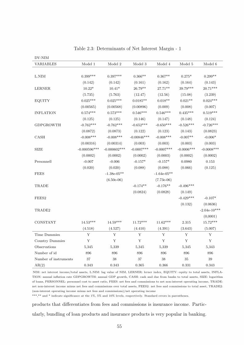
Table 2.3: Determinants of Net Interest Margin - 1

DV:NIM

VARIABLES Model 1 Model 2 Model 3 Model 4 Model 5 Model 6

L.NIM 0.399*** 0.397*** 0.366** 0.367** 0.275* 0.299**

(0.142) (0.142) (0.161) (0.162) (0.164) (0.143)

LERNER 10.22* 10.41* 26.79** 27.71** 39.79*** 20.71***

(5.735) (5.763) (12.47) (12.56) (15.08) (3.239)

EQUITY 0.025*** 0.025*** 0.0185** 0.018** 0.021** 0.024***

(0.00565) (0.00568) (0.00896) (0.009) (0.008) (0.007)

INFLATION 0.574*** 0.573*** 0.546*** 0.546*** 0.435*** 0.519***

(0.125) (0.125) (0.146) (0.147) (0.148) (0.124)

GDPGROWTH -0.762*** -0.762*** -0.652*** -0.650*** -0.526*** -0.726***

(0.0872) (0.0873) (0.122) (0.123) (0.143) (0.0823)

CASH -0.008*** -0.008*** -0.00846*** -0.008*** -0.007** -0.006*

(0.00316) (0.00314) (0.003) (0.003) (0.003) (0.003)

SIZE -0.000596*** -0.000602*** -0.0007*** -0.0007*** -0.0006*** -0.0008***

(0.0002) (0.0002) (0.0002) (0.0003) (0.0002) (0.0002)

Personnell -0.007 -0.006 -0.157* -0.157* 0.0980 0.153

(0.020) (0.020) (0.088) (0.088) (0.066) (0.125)

FEES -1.38e-05** -1.64e-05**

(6.50e-06) (7.73e-06)

TRADE -0.174** -0.176** -0.496***

(0.0824) (0.0828) (0.149)

FEES2 -0.429*** -0.107*

(0.132) (0.0636)

TRADE2 -2.04e-10***

(0,0001)

CONSTANT 14.53*** 14.59*** 11.72*** 11.62*** 2.315 15.72***

(4.518) (4.527) (4.410) (4.391) (3.643) (5.007)

Time Dummies Y Y Y Y Y Y

Country Dummies Y Y Y Y Y Y

Observations 5,345 5,339 5,345 5,339 5,345 5,343

Number of id 896 896 896 896 896 896

Number of instruments 37 38 37 38 35 39

AR(2) 0.343 0.343 0.365 0.366 0.331 0.343

NIM: net interest income/total assets, L.NIM: lag value of NIM, LERNER: lerner index, EQUITY: equity to total assets, INFLA-

TION: annual inflation rate GDPGROWTH: annual GDP growth, CASH: cash and due from banks to total assets, SIZE: logarithm

of loans, PERSONNEL: personnel cost to asset ratio, FEES: net fees and commissions to net non-interest operating income, TRADE:

net non-interest income minus net fees and commissions over total assets, FEES2: net fees and commissions to total asset, TRADE2:

(non-interest operating income minus net fees and commissions)/net operating income

***,** and * indicate significance at the 1%, 5% and 10% levels, respectively. Standard errors in parentheses.

products that differentiates from fees and commissions is insurance income. Partic-

ularly, bundling of loan products and insurance products is very popular in banking.

55

Since banks consider the gross margin and making more profit from their transac-

tions, they offer a bundle with attractive prices and connects these products. To

implement this strategy, banks lower (at least) one of the products from the bundle

in which case core product is expected to be advertised. This strategy creates a

link between trade and loan products. Otherwise, assuming a natural relationship

between these products is a low expectation, except for loss leader strategy which

is emphasized in the theoretical part. Lowering the price by loss leader strategy

is risky because even these two products may become complementary. In order to

increase the likelihood of the sale of trade products with loan products, banks may

instrument bundling as a catalytic. The insignificance of TRADENP supports the

notion of bundling strategy such that the relationship between trade income and

interest income is valid for the same period but not later. Thus, bundling creates a

link between lending activity and trade income, as well as fee income. Banks com-

pete both in the traditional and non-traditional side, and their services are typically

supplied as a bundle (Carbo and Fernandez, 2007). The absence of the individual

borrower data is a barrier to reaching certain strategies that connect these variables.

The first lag of the dependent variable is also statistically significant so that

current performance is, unsurprisingly, positively affected by past performance.

The positive and significant coefficient of LERNER appears to support the notion

that increase in market power also increases the net interest margin. Since some

banks have a market power advantage in the market, they are more flexible to

determine their interest rate, and they charge higher interest rates. Instead of

bearing higher switching cost, the customer stands these high prices.

The coefficient of the EQUITY, as expected, is positive and significant. The

positive coefficient implies the risk aversion of the bank. Banks that are unwilling to

take more risk choose higher margins to compensate higher costs of equity financing.

The alternative is external funding, and it can be more costly than equity funding

in some circumstances.

Macroeconomic factors, INFLATION and GDPGROWTH, have opposite signs

56

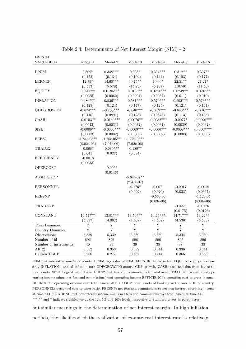
Table 2.4: Determinants of Net Interest Margin (NIM) - 2

DV:NIM

VARIABLES Model 1 Model 2 Model 3 Model 4 Model 5 Model 6

L.NIM 0.309* 0.348*** 0.303* 0.394*** 0.312** 0.397**

(0.172) (0.134) (0.169) (0.144) (0.153) (0.177)

LERNER 12.79* 14.60*** 30.75** 10.36* 22.51** 21.27*

(6.553) (5.579) (14.23) (5.787) (10.50) (11.46)

EQUITY 0.0208** 0.0185*** 0.0195** 0.0254*** 0.0249** 0.0215**

(0.0085) (0.0062) (0.0094) (0.0057) (0.011) (0.010)

INFLATION 0.486*** 0.526*** 0.581*** 0.570*** 0.502*** 0.573***

(0.125) (0.124) (0.147) (0.125) (0.121) (0.141)

GDPGROWTH -0.674*** -0.703*** -0.640*** -0.759*** -0.646*** -0.710***

(0.110) (0.0891) (0.123) (0.0873) (0.113) (0.105)

CASH -0.0103** -0.0130*** -0.0076** -0.0082*** -0.0077* -0.0096***

(0.0043) (0.0033) (0.0032) (0.0031) (0.0039) (0.0032)

SIZE -0.0006** -0.0006*** -0.0009*** -0.0006*** -0.0008*** -0.0007***

(0.0003) (0.0002) (0.0003) (0.0002) (0.0003) (0.0003)

FEES2 -1.84e-05** -1.76e-05** -1.72e-05**

(8.02e-06) (7.07e-06) (7.92e-06)

TRADE2 -0.068* -0.080*** -0.189**

(0.041) (0.027) (0.094)

EFFICIENCY -0.0018

(0.0033)

OPERCOST -0.0055

(0.0146)

ASSETSGDP -5.64e-07**

(2.41e-07)

PERSONNEL -0.176* -0.0071 -0.0017 -0.0018

(0.099) (0.020) (0.033) (0.0367)

FEESNP -9.56e-06 -1.12e-05

(6.03e-06) (8.00e-06)

TRADENP -0.0225 -0.0176

(0.0175) (0.0126)

CONSTANT 16.54*** 13.81*** 13.50*** 14.66*** 14.71*** 13.22**

(5.397) (4.062) (4.468) (4.568) (4.536) (5.533)

Time Dummies Y Y Y Y Y Y

Country Dummies Y Y Y Y Y Y

Observations 5,339 5,339 5,339 5,339 5,344 5,339

Number of id 896 896 896 896 896 896

Number of instruments 40 39 39 38 38 38

AR(2) 0.352 0.353 0.382 0.344 0.336 0.344

Hansen Test P 0.266 0.277 0.487 0.214 0.366 0.585

NIM: net interest income/total assets, L.NIM: lag value of NIM, LERNER: lerner index, EQUITY: equity/total as-

sets, INFLATION: annual inflation rate GDPGROWTH: annual GDP growth, CASH: cash and due from banks to

total assets, SIZE: Logarithm of loans, FEES2: net fees and commissions to total asset, TRADE2: (non-interest op-

erating income minus net fees and commissions)/net operating income EFFICIENCY: operating cost to gross income,

OPERCOST: operating expense over total assets, ASSETSGDP: total assets of banking sector over GDP of country,

PERSONNEL: personnel cost to asset ratio, FEESNP: net fees and commissions to net non-interest operating income

at time t+1, TRADENP: net non-interest income minus net fees and commissions over total assets at time t+1

***,** and * indicate significance at the 1%, 5% and 10% levels, respectively. Standard errors in parentheses.

but similar meanings in the determination of net interest margin. In high inflation

periods, the likelihood of the realization of ex-ante real interest rate is relatively

57

low. The uncertainty of price levels is a risk for a bank. As such, banks charge

higher interest rates in higher inflation periods. However, GDP displays a reduction

in margins. As GDP increases, banks reduce their interest margin. This negative

relationship is mainly associated with the increasing supply of funds by economic

growth. In the higher growth periods, domestic and foreign capitals may increase

and reach higher amounts of funds easier than the lower growth periods for the

banks. The third model of Table 2.4 shows that the negative coefficient of ASSETS-

GDP supports the negative link between GDPGROWTH and margin. Improvement

in the banking sector is another signal of supply of funds. As the sector improves,

available funds for banking sector increases and more funds are offered to customers

through lower interest rates.

The variable CASH is significant for all regressions and presents a negative as-

sociation. Higher liquidity reduces the liquidity risk of the banks and leads banks

to charge lower rates.

The PERSONNEL variable is employed to see the effect of personnel cost. Mod-

els state that there is an insignificant relationship between personnel cost and mar-

gin. Thus, banks do not determine their interest price subject to personnel cost.

Personnel cost increases the bank cost but on the other hand, increasing the number

of personnel may increase the performance of the bank by better provision of loans.

These two opposite effects may conflict and prevent a significant relationship.

EFFICIENCY is controlled in the first specification of Table 2.4. Result states

that interest margin is independently determined from efficiency.

Some robustness checks are also performed. First, FEES2 (net fees and commis-

sions over total asset) and TRADE2 (trade income to total net operating income

ratio) variables are introduced, and results state that they are inversely related to

interest margin, too. Second, operational cost, as another operational cost factor, is

also tested by dropping personnel cost. The second model of Table 2.4 shows that

it is also statistically insignificant to explain interest margin.

58

2.8 Conclusion

The aim of this chapter is to analyse the link between interest and non-interest in-

come components, by separately incorporating fees and trade products into Ho and

Saunders’ dealership model, in the presence of price bundling and loss leader strate-

gies and test theoretical findings for the European banking system. Specifically, in

the theoretical part, pricing strategies and conditions that satisfy the negative rela-

tionship of the lending side with trading side, as well as with fees and commissions

side, are presented. Bundling is the new trend in the banking sector, and it directly

affects traditional and non-traditional aspects of the bank revenue. One of the ad-

vantages of the bundling is offsetting the loss from one side by increasing the price

of the other side or considering gross margin rather than interest margin for profit

maximization. Moreover, bundling may enhance the market power of the bank or

reduce the total cost by spreading the fixed cost.

The increasing function of the bundling strategy motivated this study to incor-

porate it into the dealership model and create a link between income components.

Also, for the theoretical part, regarding the probability of being less-informed cus-

tomer, conditions that satisfy higher gross margin for the bank are presented. The

theoretical findings indicate that compared to the well-informed customers, in the

assumption of availability of less-informed customers, banks are able to reach higher

gross margins by underpricing the core product and charging more from fees and

commissions in loan transactions. This finding explains the banks’ advertising of

core products only or the fees and commissions’ sometimes being available as a

small-print price.

The study also empirically examines the theoretical findings. An extended ver-

sion of the bank dealership theory is tested for twelve European countries by using

System GMM method. The results state that the conditions for the negative rela-

tionship between interest income and trade income are empirically satisfied. This

negative relationship is valid for fees and commissions, too. However, the explana-

tory powers of fees and commissions and trade income are valid only for current

59

period but not the following period. These findings strengthen the possibility of

bundling, as the main strategy of the bank, to create an association between inter-

est and non-interest income aspects. Moreover, lowering the loan price for bundling

guarantees selling a non-interest product but the loss leader strategy does not guar-

antee it. Despite the strength of the possible bundling strategy, the absence of

individual borrower data is a barrier to understanding the precise reason for these

links and the weights of each strategy that contribute to these links.

The empirical results show that the past value of margin, market power, using

equity and inflation are positively associated with a higher margin. However, the

economic growth of country, liquidity of the bank and size of the loan reduce the

margin. Empirical estimations also suggest that operational expenses or personnel

expenses are insignificant to explain margin.

Individual banks that heavily concentrated on interest income due to their rev-

enue objectives should also consider the non-interest income side by mainly imple-

menting bundling strategy. However, cross-selling activities may also increase bank

risk. Therefore, cross-selling strategies are open to evaluation of risk/return trade-

off. The availability of this negative relationship should lead banks to examine their

riskiness due to the pricing strategies created this risk/return trade-off.

Further studies should focus on the weights of the pricing strategies that create

these significant relationships between lending and the non-traditional side using

the individual lending data. Understanding the pricing strategies behind these re-

lationships more clearly also helps regulators to investigate the potential banking

risks from pricing strategies. Regulations on some pricing strategies may protect

the system against potential risks.

Secondly, further studies should also consider the size effects in transactions in

any case of bundling or loss leader strategy. It is reasonable to expect that size

of the total debt may change on bundling and loss leader strategies, due to the

time differences between when transactions are carried out. In loss-leader strategy,

the overall size of the debt may be lower, compared to the simultaneous sale of

60

traditional and non-traditional products by bundling. Moreover, bundling and loss

leader strategies may affect switching costs in a different way by changing the market

power of the firm. Change in market power also affects the profitability and risk of

the bank.

Thirdly, this and other extensions of Ho and Saunders model theoretically assume

a linear demand function. Further studies can examine the non-linear demand and

supply functions.

61

2.9 Appendix A

Appendix A.1

Some Selected Bank Fees and Commissions Activities

Mortgage fee: It is fee charged for mortgage credit. It is charged when a cus-

tomer provides collateral by another mortgage for current mortgage credit appli-

cation and in finish of the payments. There are two types of fees charged under

mortgage fee. First, banks charge mortgage fee in the application to cover its cost

related to collateral. Second, banks charge fee after credit payments finish success-

fully to close collateral.

Expertise fee: When a bank customer applies for mortgage credit, banks test the

value of mortgage whether mortgage value is correct. Banks work with independent

expertise companies and test of the real value is a cost for bank. This cost is generally

charged from credit applicant. To accelerate the expertise report about real value

of the mortgage, customer may pay ”accelerated expertise fee” as well.

Booking fee: One of the most general fee types. It is related to the cost of opening

a new credit file.

Credit History Fee (Intelligence Fee): Cost of the banks stem from searching

credit history of the applicant.

Credit Allocation and Assessment Fee: Banks charge fee to cover the costs

in assessment and allocation of credit.

Flexible Payment Fee: Banks charge fee from mortgage credits if a customer

prefers flexible payment plan

Payment Plan Change Fee: If a customer requests a change in payment plan,

banks may change the plan and charge money for this alteration.

62

Advice Letter Fee: If any payment issue is available, banks send advice letter

and priced this cost to creditor.

Account fee: Banks may charge a fee for created account if application is com-

pleted successfully.

Lawyer Fee: Application and payment process may require a legal procedures

and they may charge lawyer fee.

Some Selected Trading Activities

Insurance Income Since the formula of trading activities includes all non-interest

income activities except, fees and commission income, insurance income is also as-

sumed trading activities by considering the non-interest income components in the

Bankscope database. Bankscope database differentiates fees and commissions in-

come, insurance income and all other non-interest incomes. Insurance income is an

income as a means of protection customers from financial loss.

Trading cash instruments: Trading revenue on cash and derivatives instruments

managing credit exposures includes the net gains/losses from trading cash instru-

ments and derivatives contracts that the bank manages as credit exposures, such as

debt securities and credit derivatives.

Derivative trading activities: regularly dealing in interest rate contracts, for-

eign exchange contracts, equity derivative contracts, and other off-balance sheet

commodity contracts

Cash instruments: the net gain or loss from trading cash instrument

Foreign Exchange: the net gain or loss from foreign exchange

63

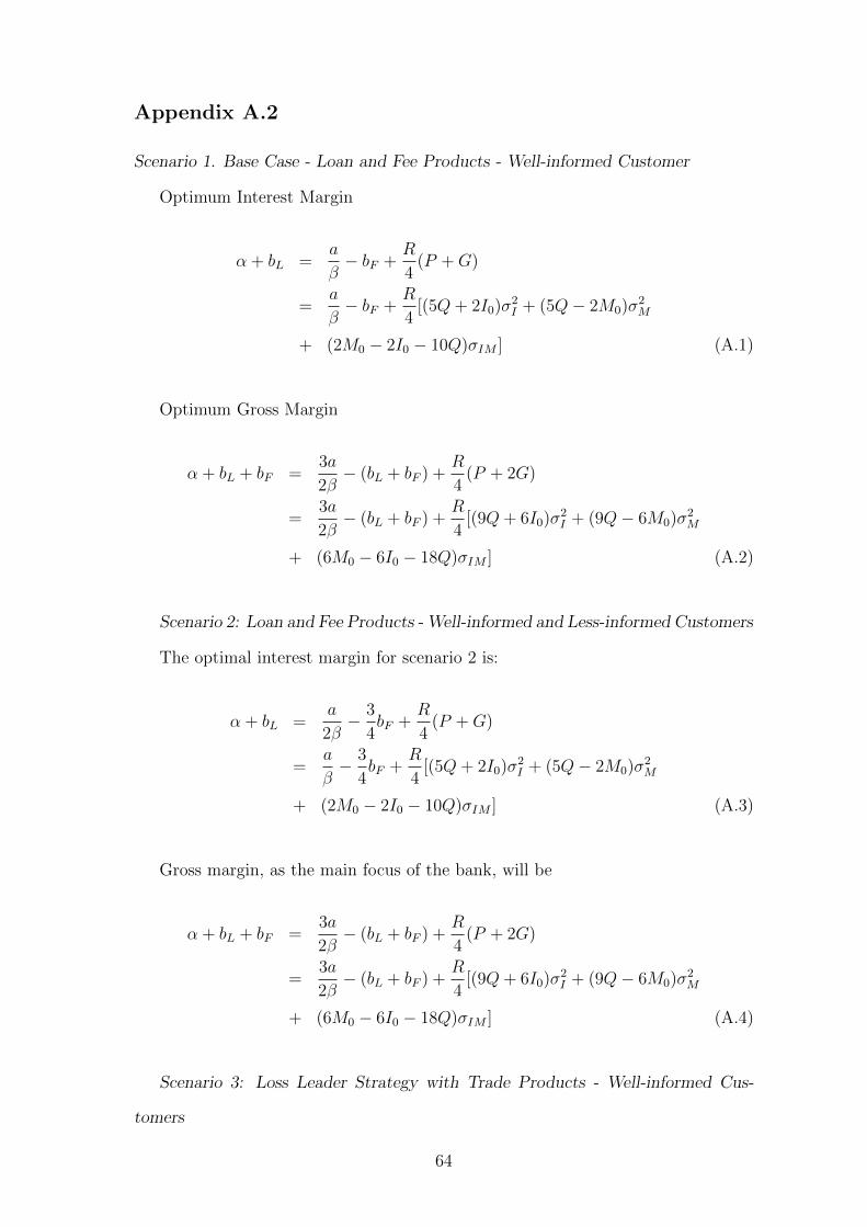
Appendix A.2

Scenario 1. Base Case - Loan and Fee Products - Well-informed Customer

Optimum Interest Margin

α + bL =a

β− bF +

R

4(P +G)

=a

β− bF +

R

4[(5Q+ 2I0)σ2

I + (5Q− 2M0)σ2M

+ (2M0 − 2I0 − 10Q)σIM ] (A.1)

Optimum Gross Margin

α + bL + bF =3a

2β− (bL + bF ) +

R

4(P + 2G)

=3a

2β− (bL + bF ) +

R

4[(9Q+ 6I0)σ2

I + (9Q− 6M0)σ2M

+ (6M0 − 6I0 − 18Q)σIM ] (A.2)

Scenario 2: Loan and Fee Products - Well-informed and Less-informed Customers

The optimal interest margin for scenario 2 is:

α + bL =a

2β− 3

4bF +

R

4(P +G)

=a

β− 3

4bF +

R

4[(5Q+ 2I0)σ2

I + (5Q− 2M0)σ2M

+ (2M0 − 2I0 − 10Q)σIM ] (A.3)

Gross margin, as the main focus of the bank, will be

α + bL + bF =3a

2β− (bL + bF ) +

R

4(P + 2G)

=3a

2β− (bL + bF ) +

R

4[(9Q+ 6I0)σ2

I + (9Q− 6M0)σ2M

+ (6M0 − 6I0 − 18Q)σIM ] (A.4)

Scenario 3: Loss Leader Strategy with Trade Products - Well-informed Cus-

tomers

64

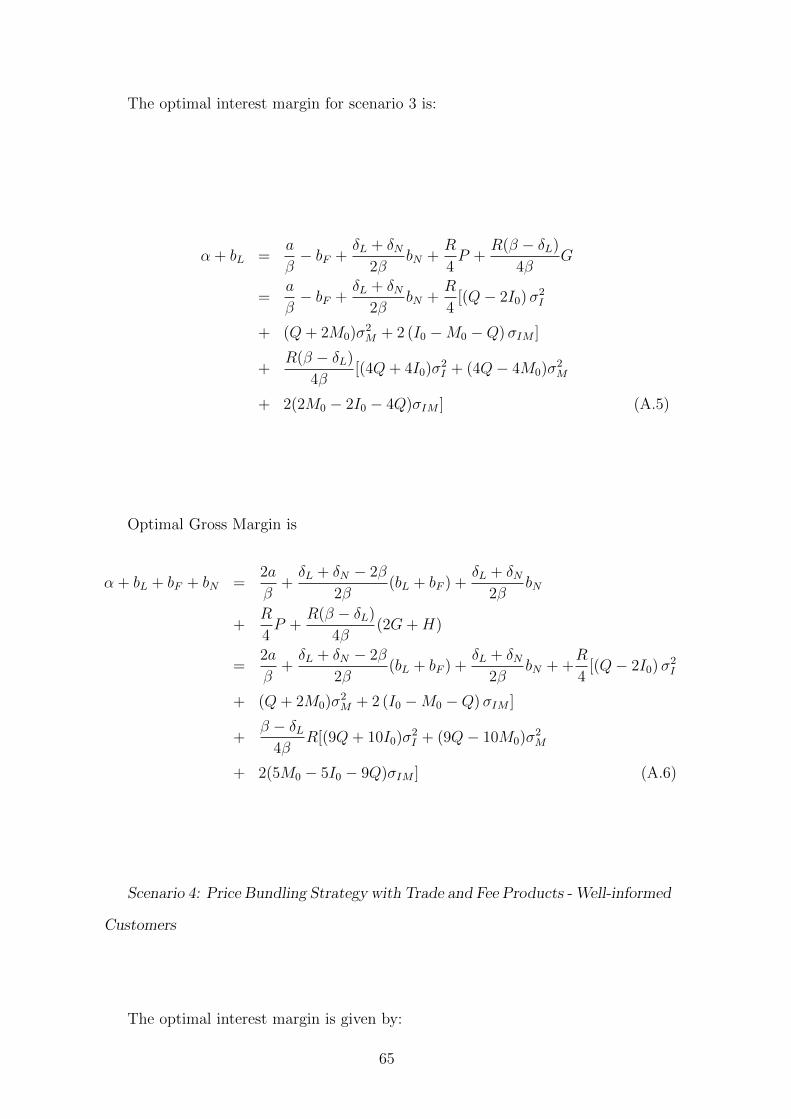
The optimal interest margin for scenario 3 is:

α + bL =a

β− bF +

δL + δN2β

bN +R

4P +

R(β − δL)

4βG

=a

β− bF +

δL + δN2β

bN +R

4[(Q− 2I0)σ2

I

+ (Q+ 2M0)σ2M + 2 (I0 −M0 −Q)σIM ]

+R(β − δL)

4β[(4Q+ 4I0)σ2

I + (4Q− 4M0)σ2M

+ 2(2M0 − 2I0 − 4Q)σIM ] (A.5)

Optimal Gross Margin is

α + bL + bF + bN =2a

β+δL + δN − 2β

2β(bL + bF ) +

δL + δN2β

bN

+R

4P +

R(β − δL)

4β(2G+H)

=2a

β+δL + δN − 2β

2β(bL + bF ) +

δL + δN2β

bN + +R

4[(Q− 2I0)σ2

I

+ (Q+ 2M0)σ2M + 2 (I0 −M0 −Q)σIM ]

+β − δL

4βR[(9Q+ 10I0)σ2

I + (9Q− 10M0)σ2M

+ 2(5M0 − 5I0 − 9Q)σIM ] (A.6)

Scenario 4: Price Bundling Strategy with Trade and Fee Products - Well-informed

Customers

The optimal interest margin is given by:

65

α + bL =a

β− bF −

bN + u

2+R

8(2P +G+ J) +

RδL8β

H

=a

β− bF −

bN + u

2+R

4[(Q− 2I0)σ2

I + (Q+ 2M0)σ2M

+ 2 (I0 −M0 −Q)σIM ] +R

8[(15Q+ 6I0)σ2

I + (15Q− 6M0)σ2M

+ 2 (3M0 − 3I0 − 15Q)σIM ]

+ RδL8β

[(Q+ 2I0)σ2I + (Q− 2M0)σ2

M + (2M0 − 2I0 − 2Q)σIM ] (A.7)

Gross margin, as the main focus of the bank

α + bL + bF + bN =2a

β− 3

2(bL + bF − u)− bN +

R

4(P +G+ J)

+R(2δL + δN)

8βH

=2a

β− 3

2(bL + bF − u)− bN +

R

2[(7Q+ 4I0)σ2

I

+ (7Q− 4M0)σ2M + 2(2M0 − 2I0 − 7Q)σIM ] (A.8)

66

Chapter 3

Switching Cost Effect of

Long-term Loan in Cross Selling

Abstract

The purpose of this study is to investigate the switching cost effect of long-term loans

on selling non-interest products. The study builds on the theoretical framework sug-

gested by Kim et al. (2003) and its extensions in the literature. A theoretical model

is developed to explain the switching cost for non-interest products in relation to

long-term loans. The study provides an empirical test of the theoretical model using

unique banking data from the UK banking sector covering the period 2005 - 2012.

The results confirm that banks create a switching cost for non-interest product mar-

ket by keeping interest rates level low enough for long-term loans and thus, locking

the customers in for longer periods by shifting loans from short-term to long-term.

The results reveal that switching cost by loan maturity have implications for bank

management and regulators regarding banks profitability and the risk associated

with switching cost for cross-selling.

67

3.1 Introduction

The relationship between banks and customers have undergone significant transfor-

mations in the last three decades. Dealing with banks became a necessity rather

than a luxury for daily aspects for both individuals and businesses. Many factors

contributed to such transformation among others the technology advancement; in-

creasing competition; and progression in communications.

Accordingly, banks have tried to initiate new strategies to maximize their profits.

One of these strategies is selling non-traditional products to the customers. Banks

have used their traditional product as an instrument to promote the non-traditional

side of the business to customers. In the sense that by selling a traditional product,

it creates a planned path to the non-traditional product sale. In the process of

building such bridge between the traditional and non-traditional products, banks

implement pricing strategies to sell both types of products to the same customer.

Selling non-traditional products and services to the loan customer, however, may

require time or at least, a likelihood of selling non-traditional products and services

to the loan customer rises over time. At this point, the long-term loan appears

to be an excellent opportunity for banks to achieve this goal. The long-term loan

allows banks to improve their communication thus persuading customers to buy

non-interest products and services from that bank. Moreover, the bank may use

available customer information to forecast their consumption pattern. Kane and

Malkiel (1965) and Fama (1985) argue that a bank which lends to a firm obtain

more information about borrower’s characteristics. Doing so, banks may intend

to create a switching cost through long-term loans. They may attract customer

by underpricing interest rate level as a first step to creating a switching cost. In

another perspective, a higher switching cost arise once a bank initially engages in a

loan agreement, thus opening the gate of selling a planned non-traditional products

and services. A switching cost is a form of market power for the bank to increase

its price (Klemperer, 1995). Thus, by locking the customer in and creating market

power, banks can offset this loss with non-traditional product and service sale with

68

higher prices in the future.

Profitability and riskiness of banks are two main factors of banks’ financial sound-

ness, particularly after the recent global financial crisis. Creating switching cost by

lowering long-term loan prices directly affects the profitability of banks. Therefore,

the factors that influence financial soundness become more of an issue. Moreover,

income sources are of great importance for banks, as most of the empirical studies in

the literature discuss increasing risk caused by income diversification (Stiroh, 2004;

Le Petit et al., 2008), even income diversification is known by risk reducing prop-

erty. This need to risk associated with income diversification usually implies the

cross-selling strategies of banks. Strategies and relations that provide cross-selling

for banks are highly crucial. In this point, the potential switching cost effect of long

term loans for non-traditional product sale is critical for banks as well as regula-

tors. Its importance increase when the magnitude of long-term loans is considered,

which implies that higher size loans are more risky. There is abundant literature on

switching cost, including those which have focused on the effect of the loan price and

those which have examined internal and external information asymmetry. However,

none of the studies highlight the switching cost effect of loan maturity, particularly

considering long-term loan, despite the fact that switching cost is a longer period

phenomenon. This study fills the gap in the literature by theoretically incorporating

the switching cost effect of long term loans for non-traditional products and empir-

ically examines the theoretical contribution for the UK banking system. Banks in

the UK are less regional, state, co-operative or mutual banks hence; they are likely

to adopt profit maximizing pricing and cross-selling strategies. Furthermore, com-

pared to European countries, for the period that this study examines, 2005 - 2012,

the UK banks were heavily reliant on non-interest income. Greater reliance on non-

interest income in the UK banking system provides an incentive to test switching

cost strategies for non-interest products.

The contribution of this study is twofold. First, this study theoretically ex-

tends the switching cost model set up in Kim et al. (2003) and extended by Zhao

69

et al. (2013), by incorporating the switching cost effect of long term loan for non-

traditional product sale or shortly loanavity effect1. Second, this study tests the

theoretical foundation associated with switching cost effect of loan maturity for the

UK banking system over the period 2005 - 2012. According to the results, switching

cost for non-traditional products increases by shifting of loans from short-term to

long-term. The study also specifically examines the relationship between long-term

loan and trade products, due to the potential differences seen between broad non-

interest product category and trade products. The results confirm that a similar

relationship is valid for trade products as well. Switching cost is created even for

longer periods for trade products.

The rest of the chapter proceeds as follows: Section 3.2 of the study is comprised

of a literature review on the effect of switching cost on bank strategy. Section 3.3

presents the extended version of the switching cost model. Section 3.4 describes

the data. Section 3.5 defines and explains the dependent and independent variables

used in regression analysis. Section 3.6 analyses the econometric method used in

the regression models; non-linear three stages least square. Section 3.7 includes

regression results and their analysis. Section 3.8 concludes.

3.2 Literature Review

The assessment of switching cost in the banking sector is of considerable interest

to researchers. Klemperer (1987) explains market share by introducing switch cost

as an instrument for corporate strategy. Ausubel (1991) examines the credit card

interest rates and finds that credit card interest rates have been sticky relative to the

cost of funds over the period 1983 and 1988. The switching cost is the candidate of

a sticky interest rate due to the difficulties in locating banks which offer favourable

rates. Borenstein (1991) finds that gas stations create price discrimination against

the customer who has a lower likelihood of switching to another station. The author

1loanavity the author created expression. The etymology of the word loanavity lies with thewords loan and gravity combined. Loanavity is an inertia that increasing with loan maturity topurchase non-interest products and services from bank that customer purchase loan product

70

emphasizes the importance of unwillingness to switch rival firm due to the switching

cost. Barone et al. (2011), by using bank-firm level data on four Italian local credit

markets, show that firms changing their main lender exposes them to significant

switching costs. On average, 70 percent of the customers continue to choose the

previous period main borrower bank as the current main borrower.

Some of the studies empirically compare the rates offered by the inside and

outside banks, but there is no consensus on results. Ioannidou and Ongena (2010)

compare the inside, and outside bank interest rates offered using the Bolivian credit

registry between 1999 and 2003. The inside interest rate is the interest rate provided

by the current bank and outside interest rates are the new bank’s interest rate offered

to the customer. They find that interest rate is reduced by new banks in case of

switching. However, new banks increase their interest rate sharply in the following

periods. The study also finds that new bank turns to starting point interest rate

after around three years. Black (2006), by analysing the US Survey of Small Business

Finance, empirically finds that outsider firms offer higher than insider firm. Outside

loan rates are 40 basis, on average, higher than inside/current bank. However,

Barone et al. (2006) find that switched customers pay lower i.e. between 25 and 123

base points.

One part of the literature tests the loan price and relationship time associa-

tion. Petersen and Rajan (1994) find that loan rates are independent of relationship

time. Berger (1995) find that loan price is negatively associated with relationship

time which is evidence against hold-up. Whereas, some other studies find results

consistent with hold-up hypothesis such that loan price increases in accordance with

time (Degryse and Ongena, 2005). Ongena and Smith (2001) and, Farinha and San-

tos (2002) highlights the importance of duration from a different perspective. They

find that probability of replacing the bank increases in duration. The number of

the banks that a customer has accounts with negatively affects the length of the

relationship. The study also finds that high growth and leveraged firms switch their

banks faster.

71

Another part of the empirical foundations is the amount of switching cost. Kim

et al. (2003) empirically found that switching costs are about one-third of the average

interest rate on loans. According to Shy (2002), data on price and market shares

show that cost of switching between banks varies 0 to 11% of the average balance

in the Finland market for bank accounts.

Gopalan et al. (2007) analyse the firm motivation for switching to a new bank

by using micro-data. According to the authors, the main motivation for changing

a bank are borrowing constraints. Hence, firms prefer to switch to another bank to

obtain larger loan size. They find that firms are more likely to switch from small

banks to large banks. The most opaque (transparent) a firm the highly (least) likely

it will switch their banks.

Some studies make a theoretical contribution to the literature. Padilla (1992)

develops a model in terms of which functionally identical products, ex-ante ho-

mogenous, become heterogeneous products through the presence of switching cost.

Thus, ex-ante homogenous products are transformed to a differentiated product by

switching cost. Sharpe (1990) theorizes the bank loan market in the presence of

information asymmetry by considering inside versus outside lending. He elaborates

that, a lender obtains private information about a firm in the process of giving credit.

There are two periods in his model, in the first period, banks compete to win the

borrower. They have only publicly available information. One of the banks wins

the competition and lends to a customer. This bank obtains private information

about the customer by observing the payments during the first period. The firm is

defined as a good firm, if the firm makes payments successfully, however, the firm

is defined as a bad firm, if they defaulted on the loan. Then, in the second period,

competition changes due to the private information obtained by the lender bank

or now the informed side lender. The informed side lender offers to the customer

by considering the private information, whereas, other banks offer without having

private information which places them at a disadvantage. In another study, Von

Thadden (2004), shows that a unique, mixed strategy equilibrium can exist for the

72

second-period of competition. The outside or uninformed lender regards the possi-

bility of winner’s curse. By offering a lower rate, they can win but attract mostly

the bad firms. The insider firm offers low-interest for the good firms and high ones

for the bad firms. In this case, the outside firm is mostly preferred by bad firms. To

win some of the good firms, the outside lender needs to randomize its offer strategy.

The insider lender, like the outside lender, randomizes to earn a higher rate on each

offer that it wins.

Kim et al. (2003) seminal work, introduces the theoretically structural model,

for switching cost as a factor of price-cost margin and bank loan share. A bank

determines its pricing strategy by considering future periods and thus, future profits

are determined by the current period pricing strategy of the bank. Bank alleviates its

price to attract customers. Once the relation with the borrower is established, bank

enhances its price in the following periods, when they lock these customers in. Thus,

the strategy is offsetting the loss from lowering prices by creating switching cost over

time. The study examines the effect of switching cost on price-cost margin. The

effect of non-interest income is not the motivation of this study. They empirically

test the magnitude of theoretical findings in Norwegian credit markets by analysing

aggregate market shares and interest price over the period 1988 and 1996.

On the other hand, some other studies show that banks determine their loan

price not only considering loan market conditions or future periods but also con-

sidering non-interest income. Banks lower their loan price by compensating it with

cross-selling (Carbo and Fernandez, 2007; Lepetit et al., 2008; Maudos and Solis,

2009). The findings of these studies show that loan pricing is negatively associated

with fees and commissions, but trade income is insignificant to explain interest mar-

gin. For this strategy, Farrell and Klemperer (2007) state that multi-product firms

advertise their core product, but they also expect that core product customers also

purchase non-core products, too. Zhao et al. (2013)’s theoretical study combines the

effect of non-interest income, competition and switching cost on loan pricing. The

study introduces a switching probability associated with non-interest income to ex-

73

amine the factors affecting the switching for non-interest products. The theoretical

findings were empirically tested for the UK banking system over the period 1993 -

2008. Their empirical results show that banks charge more from the customers who

faced high switching costs in the loan market in the latter period. As a result, the

period 2000 - 2008 is considered a relatively weaker period of competitiveness in the

banking sector. They also find that competitiveness and cross-selling are negatively

associated with British banks.

3.3 Theoretical Model

3.3.1 Kim’s Model

The model assumes that there are some n banks operating in oligopoly and banks

compete in a multiple stage pricing. Banks determine their price by considering

each stage. Though multi-stage pricing is available, the model assumes that the

good sold by the bank is unstorable and thus selling them later is not an option.

Customers have inelastic demand in purchasing the good. There are infinite periods

during which each customer can buy a single unit of the goods for these periods.

Each side maximises their utility. For demand side, customer compares the price

offered by banks and then, they pick out one of them to buy the loan. One of

the primary considerations of Kim et al. (2003) model is that customers consider

the switching cost among banks when they compare the prices of each bank. The

existence of switching cost creates a barrier for customers to change their bank. This

switching cost implies significantly higher probabilities of staying at the same bank

than transitioning to another bank.

The transition probabilities from one bank to another are the demand side of

the maximization problem. Price and switching cost are two factors that impact

the bank selection and model considers these factors in transition probabilities.

The maximization problem models the customer decision by considering price and

switching cost, as well as the likelihood of potential purchase from one of the rival

74

banks in the market. In this theory, transition probabilities are Markovian. The

switching cost is incorporated into the model by addition to the price.

If a customer stays at the same bank for the next period, it is stated by Pri→i,t.

However, bank i may attract customer from bank j and its switching probability is

denoted by Prj→i,t. These probabilities are the functions of prices charged by bank

and switching cost. Loan price of the bank i at time t is denoted by pl,i,t. Prices

of rival banks are also impact the probabilities due to the cross-price elasticity and

it is a (n-1) vector pl,i,R,t. The probability of staying at the same bank rather than

switching to another bank is formulated as:

Pri→i,t = f(pl,i,t, pl,i,R,t + s) (3.1)

where s is a n-1 vector of switching cost and it equals the multiplication of scalar s

and (n-1) unity vector: s ≡ s · I.

Customers do not have to stay at the same bank forever. The likelihood of

switching from a rival bank j to bank i is given by:

Prj→i,t = f(pl,i,t + s, pl,i,R,t + sj) (3.2)

where sj is an (n-1) vector of switching cost. Jth element of vector is 0 but all others

are equals s.

In aggregate, transitions are unobserved. Thus, formulation of the probability

of switching to purchase loan from bank i unconditional on the rival’s identity, is

given by:

PriR→i,t =∑

f(pl,i,t + s, pl,i,R,t + sj)yl,j,t−1∑k 6=i yl,k,t−1

(3.3)

where PriR→i,t is switching of rival’s customer to bank i. yl,j,t−1 is the output of

75

bank j at time t-1. The probability of purchasing loan by customer of a randomly

selected bank that rival to bank i is the one who purchased previously from bank j

is yl,j,t−1/Σk 6=iyl,k,t−1

Total demand for bank i is equal to the bank i ’s previous period output with

staying probability and new comers from its rivals with transition probability. Out-

put of bank i at time t is:

yl,i,t = yl,i,t−1Pri→i,t + yl,i,R,t−1Pri,R→i,t (3.4)

The first term is the estimation of keeping old customers at bank i, calculated by

multiplication of the previous period output with probability of staying and second

term is the estimation of the output stem from new customers and is calculated

by potential demand coming from rivals’ customers and transition probability. So,

estimated total demand is the sum of the demand of the old customers and demand

of customers who switch from rival banks. It is also necessary that market capacity

changes with respect to factors, i.e. macroeconomic conditions, from one year to

another. Therefore, total demand faced by bank i is also affected by loan market

growth. Formulated total output is given by:

yl,i,t = [yl,i,t−1Pri→i,t + yl,i,R,t−1Pri,R→i,t]gt (3.5)

where gt is the market growth rate, gt ≡∑yl,i,t∑yl,i,t−1

. Market growth rate is exogenous

for this model.

Having the aggregate data prevents banks from observing each customer’s trans-

actions and the arrival or switch of customers. Thus, banks are unable to observe

actual customer decisions. In the absence of observing each customer decision, net

output changes presented by the aggregate data are used. Therefore, theory derives

a demand that depends on market share of banks. To create this connection, first

76

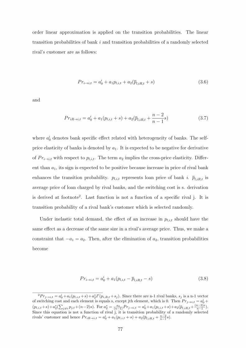
order linear approximation is applied on the transition probabilities. The linear

transition probabilities of bank i and transition probabilities of a randomly selected

rival’s customer are as follows:

Pri→i,t = ai0 + a1pl,i,t + a2(pl,iR,t + s) (3.6)

and

PriR→i,t = ai0 + a1(pl,i,t + s) + a2(pl,iR,t +n− 2

n− 1s) (3.7)

where ai0 denotes bank specific effect related with heterogeneity of banks. The self-

price elasticity of banks is denoted by a1. It is expected to be negative for derivative

of Pri→i,t with respect to pl,i,t. The term a2 implies the cross-price elasticity. Differ-

ent than a1, its sign is expected to be positive because increase in price of rival bank

enhances the transition probability. pl,i,t represents loan price of bank i. pl,iR,t is

average price of loan charged by rival banks, and the switching cost is s. derivation

is derived at footnote2. Last function is not a function of a specific rival j. It is

transition probability of a rival bank’s customer which is selected randomly.

Under inelastic total demand, the effect of an increase in pl,i,t should have the

same effect as a decrease of the same size in a rival’s average price. Thus, we make a

constraint that −a1 = a2. Then, after the elimination of a2, transition probabilities

become

Pri→i,t = ai0 + a1(pl,i,t − pl,iR,t − s) (3.8)

2Prj→i,t = ai0 +a1(pl,i,t +s)+a∗2I′(pi,R,t +sj). Since there are n-1 rival banks, sj is a n-1 vector

of switching cost and each element is equals s, except jth element, which is 0. Then Prj→i,t = ai0 +

(pl,i,t+s)+a∗2(∑

j 6=i pj,t+(n−2)s). For a∗2 = a2

(n−1)Prj→i,t = ai0+a1(pl,i,t+s)+a2(pl,iR,t+(n−2)sn−1 ).

Since this equation is not a function of rival j, it is transition probability of a randomly selectedrivals’ customer and hence PriR→i,t = ai0 + a1(pl,i,t + s) + a2(pl,iR,t + n−2

n−1s).

77

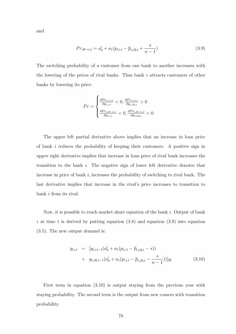
and

PriR→i,t = ai0 + a1(pl,i,t − pl,iR,t +s

n− 1) (3.9)

The switching probability of a customer from one bank to another increases with

the lowering of the prices of rival banks. Thus bank i attracts customers of other

banks by lowering its price:

Pr =

∂Pri→i,t

∂pl,i,t< 0,

∂Pri→i,t

∂pl,iR,t> 0

∂Pri,R→i,t

∂pl,i,t< 0,

∂Pri,R→i,t

∂pl,iR,t> 0

The upper left partial derivative above implies that an increase in loan price

of bank i reduces the probability of keeping their customers. A positive sign in

upper right derivative implies that increase in loan price of rival bank increases the

transition to the bank i. The negative sign of lower left derivative denotes that

increase in price of bank i, increases the probability of switching to rival bank. The

last derivative implies that increase in the rival’s price increases to transition to

bank i from its rival.

Now, it is possible to reach market share equation of the bank i. Output of bank

i at time t is derived by putting equation (3.8) and equation (3.9) into equation

(3.5). The new output demand is:

yl,i,t = [yl,i,t−1(ai0 + a1(pl,i,t − pl,iR,t − s))

+ yl,iR,t−1(ai0 + a1(pl,i,t − pl,iR,t −s

n− 1))]gt (3.10)

First term in equation (3.10) is output staying from the previous year with

staying probability. The second term is the output from new comers with transition

probability.

78

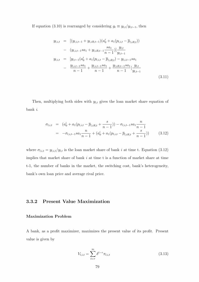
If equation (3.10) is rearranged by considering gt ≡ yl,t/yl,t−1, then

yl,i,t = [(yl,i,t−1 + yl,iR,t−1)(ai0 + a1(pl,i,t − pl,iR,t))

− (yl,i,t−1sa1 + yl,iR,t−1sa1

n− 1)]yl,tyl,t−1

yl,i,t = [yl,t−1(ai0 + a1(pl,i,t − pl,iR,t)− yl,i,t−1sa1

− yl,i,t−1sa1

n− 1+yl,i,t−1sa1

n− 1+yl,iR,t−1sa1

n− 1]yl,tyl,t−1

(3.11)

Then, multiplying both sides with yl,t gives the loan market share equation of

bank i.

σl,i,t = (ai0 + a1(pl,i,t − pl,iR,t +s

n− 1))− σl,i,t−1sa1

n

n− 1

= −σl,i,t−1sa1n

n− 1+ (ai0 + a1(pl,i,t − pl,iR,t +

s

n− 1)) (3.12)

where σl,i,t = yl,i,t/yl,t is the loan market share of bank i at time t. Equation (3.12)

implies that market share of bank i at time t is a function of market share at time

t-1, the number of banks in the market, the switching cost, bank’s heterogeneity,

bank’s own loan price and average rival price.

3.3.2 Present Value Maximization

Maximization Problem

A bank, as a profit maximizer, maximizes the present value of its profit. Present

value is given by

Vl,i,t =∞∑t=τ

δt−τπl,i,t (3.13)

79

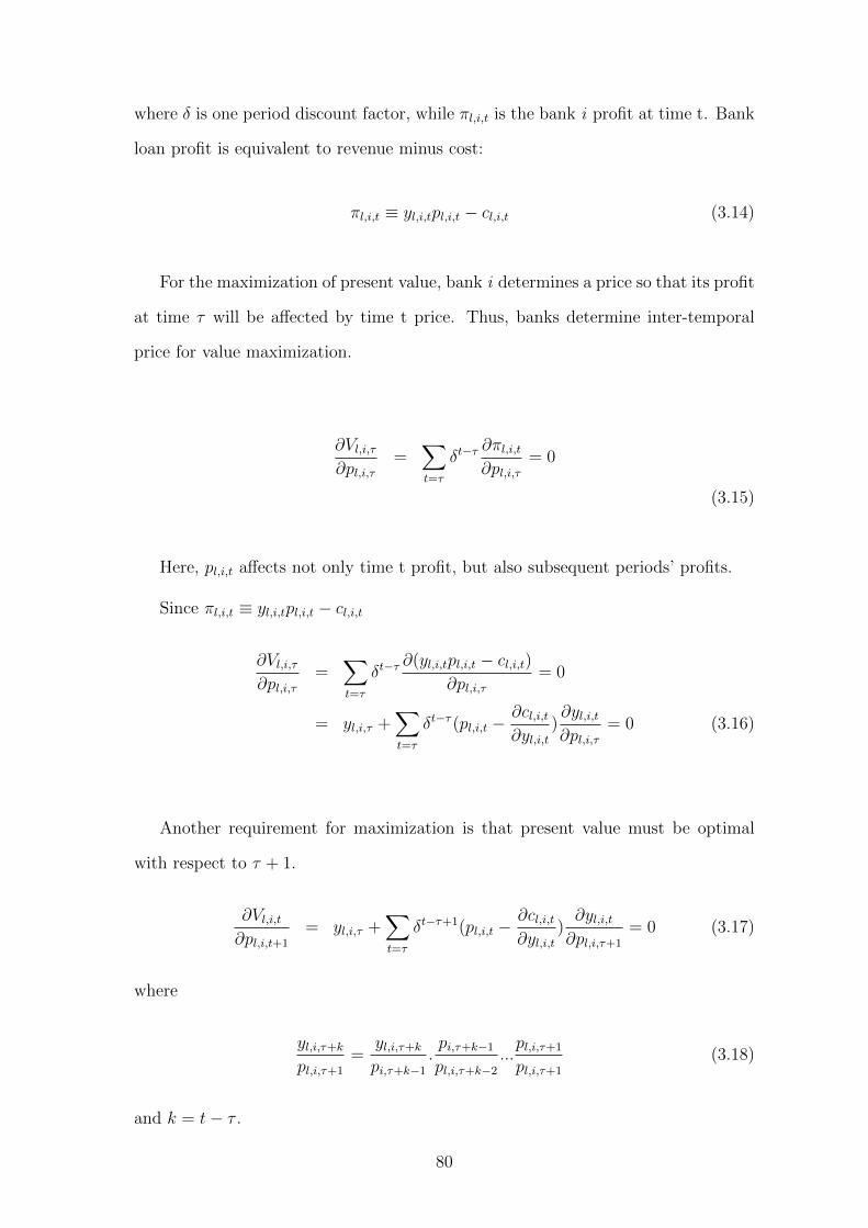
where δ is one period discount factor, while πl,i,t is the bank i profit at time t. Bank

loan profit is equivalent to revenue minus cost:

πl,i,t ≡ yl,i,tpl,i,t − cl,i,t (3.14)

For the maximization of present value, bank i determines a price so that its profit

at time τ will be affected by time t price. Thus, banks determine inter-temporal

price for value maximization.

∂Vl,i,τ∂pl,i,τ

=∑t=τ

δt−τ∂πl,i,t∂pl,i,τ

= 0

(3.15)

Here, pl,i,t affects not only time t profit, but also subsequent periods’ profits.

Since πl,i,t ≡ yl,i,tpl,i,t − cl,i,t

∂Vl,i,τ∂pl,i,τ

=∑t=τ

δt−τ∂(yl,i,tpl,i,t − cl,i,t)

∂pl,i,τ= 0

= yl,i,τ +∑t=τ

δt−τ (pl,i,t −∂cl,i,t∂yl,i,t

)∂yl,i,t∂pl,i,τ

= 0 (3.16)

Another requirement for maximization is that present value must be optimal

with respect to τ + 1.

∂Vl,i,t∂pl,i,t+1

= yl,i,τ +∑t=τ

δt−τ+1(pl,i,t −∂cl,i,t∂yl,i,t

)∂yl,i,t∂pl,i,τ+1

= 0 (3.17)

where

yl,i,τ+k

pl,i,τ+1

=yl,i,τ+k

pi,τ+k−1

.pi,τ+k−1

pl,i,τ+k−2

...pl,i,τ+1

pl,i,τ+1

(3.18)

and k = t− τ .

80

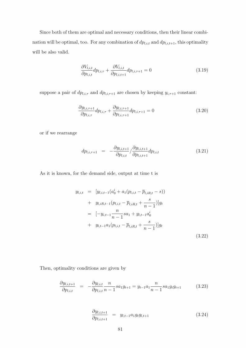
Since both of them are optimal and necessary conditions, then their linear combi-

nation will be optimal, too. For any combination of dpl,i,t and dpl,i,t+1, this optimality

will be also valid.

∂Vl,i,t∂pl,i,t

dpl,i,τ +∂Vl,i,t∂pl,i,t+1

dpl,i,τ+1 = 0 (3.19)

suppose a pair of dpl,i,τ and dpl,i,τ+1 are chosen by keeping yi,τ+1 constant:

∂yl,i,τ+1

∂pl,i,τdpl,i,τ +

∂yl,i,τ+1

∂pl,i,τ+1

dpl,i,τ+1 = 0 (3.20)

or if we rearrange

dpl,i,τ+1 = −∂yl,i,t+1

∂pl,i,t/∂yl,i,t+1

∂pl,i,t+1

dpl,i,t (3.21)

As it is known, for the demand side, output at time t is

yl,i,t = [yl,i,t−1(ai0 + a1(pl,i,t − pl,iR,t − s))

+ yl,iR,t−1(pl,i,t − pl,iR,t +s

n− 1)]gt

= [−yi,t−1n

n− 1sa1 + yl,t−1a

i0

+ yl,t−1a1(pl,i,t − pl,iR,t +s

n− 1)]gt

(3.22)

Then, optimality conditions are given by

∂yl,i,t+1

∂pl,i,t= −∂yl,i,t

∂pl,i,t

n

n− 1sa1gt+1 = yt−1a1

n

n− 1sa1gtgt+1 (3.23)

∂yl,i,t+1

∂pl,i,t+1

= yl,t−1a1gtgl,t+1 (3.24)

81

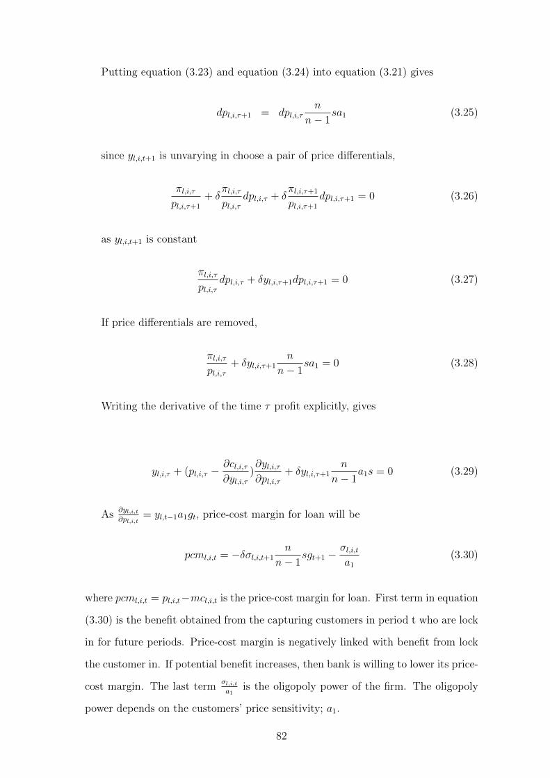
Putting equation (3.23) and equation (3.24) into equation (3.21) gives

dpl,i,τ+1 = dpl,i,τn

n− 1sa1 (3.25)

since yl,i,t+1 is unvarying in choose a pair of price differentials,

πl,i,τpl,i,τ+1

+ δπl,i,τpl,i,τ

dpl,i,τ + δπl,i,τ+1

pl,i,τ+1

dpl,i,τ+1 = 0 (3.26)

as yl,i,t+1 is constant

πl,i,τpl,i,τ

dpl,i,τ + δyl,i,τ+1dpl,i,τ+1 = 0 (3.27)

If price differentials are removed,

πl,i,τpl,i,τ

+ δyl,i,τ+1n

n− 1sa1 = 0 (3.28)

Writing the derivative of the time τ profit explicitly, gives

yl,i,τ + (pl,i,τ −∂cl,i,τ∂yl,i,τ

)∂yl,i,τ∂pl,i,τ

+ δyl,i,τ+1n

n− 1a1s = 0 (3.29)

As∂yl,i,t∂pl,i,t

= yl,t−1a1gt, price-cost margin for loan will be

pcml,i,t = −δσl,i,t+1n

n− 1sgt+1 −

σl,i,ta1

(3.30)

where pcml,i,t = pl,i,t−mcl,i,t is the price-cost margin for loan. First term in equation

(3.30) is the benefit obtained from the capturing customers in period t who are lock

in for future periods. Price-cost margin is negatively linked with benefit from lock

the customer in. If potential benefit increases, then bank is willing to lower its price-

cost margin. The last termσl,i,ta1

is the oligopoly power of the firm. The oligopoly

power depends on the customers’ price sensitivity; a1.

82

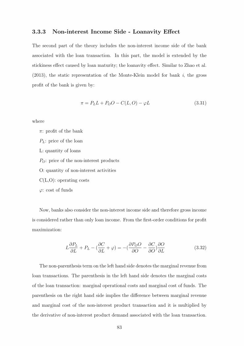
3.3.3 Non-interest Income Side - Loanavity Effect

The second part of the theory includes the non-interest income side of the bank

associated with the loan transaction. In this part, the model is extended by the

stickiness effect caused by loan maturity; the loanavity effect. Similar to Zhao et al.

(2013), the static representation of the Monte-Klein model for bank i, the gross

profit of the bank is given by:

π = PLL+ POO − C(L,O)− ϕL (3.31)

where

π: profit of the bank

PL: price of the loan

L: quantity of loans

PO: price of the non-interest products

O: quantity of non-interest activities

C(L,O): operating costs

ϕ: cost of funds

Now, banks also consider the non-interest income side and therefore gross income

is considered rather than only loan income. From the first-order conditions for profit

maximization:

L∂PL∂L

+ PL − (∂C

∂L+ ϕ) = −(

∂POO

∂O− ∂C

∂O)∂O

∂L(3.32)

The non-parenthesis term on the left hand side denotes the marginal revenue from

loan transactions. The parenthesis in the left hand side denotes the marginal costs

of the loan transaction: marginal operational costs and marginal cost of funds. The

parenthesis on the right hand side implies the difference between marginal revenue

and marginal cost of the non-interest product transaction and it is multiplied by

the derivative of non-interest product demand associated with the loan transaction.

83

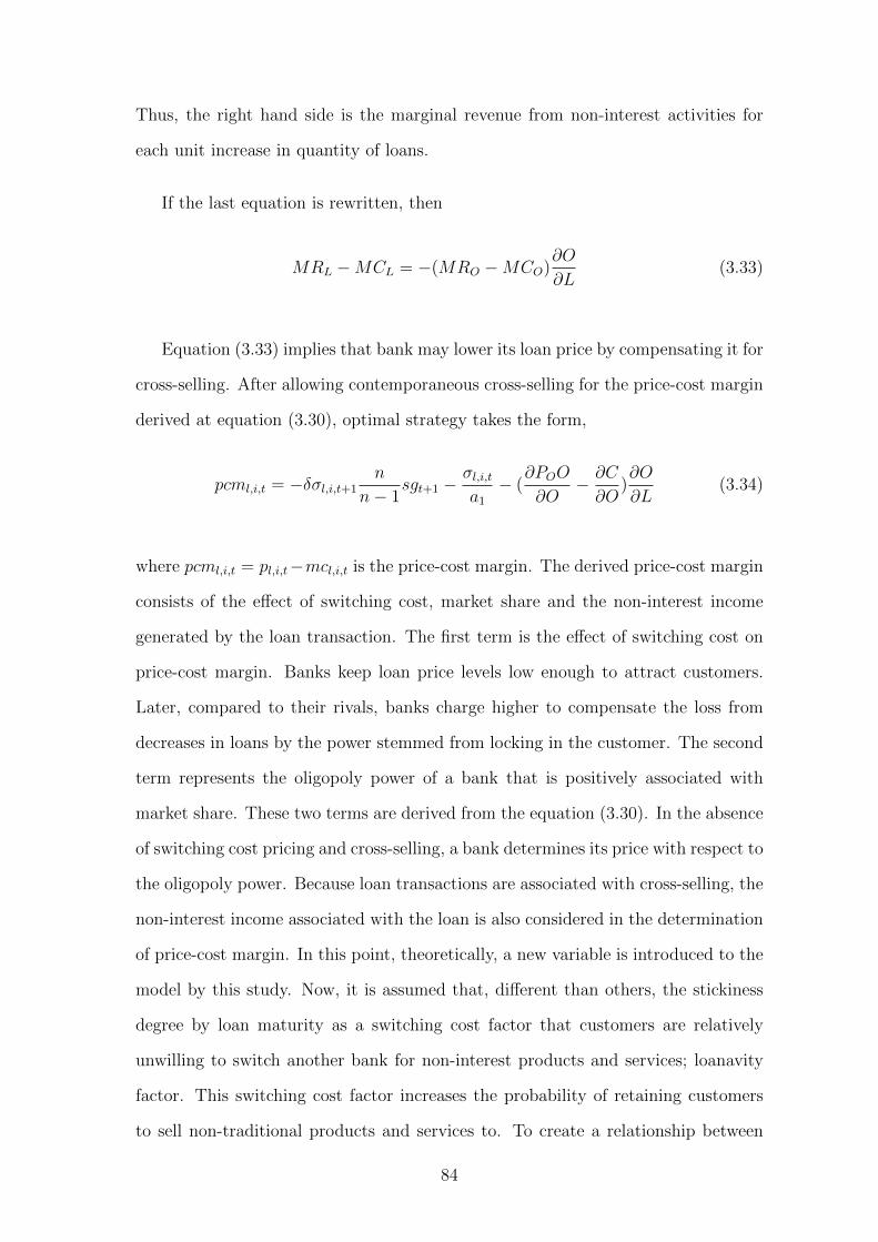
Thus, the right hand side is the marginal revenue from non-interest activities for

each unit increase in quantity of loans.

If the last equation is rewritten, then

MRL −MCL = −(MRO −MCO)∂O

∂L(3.33)

Equation (3.33) implies that bank may lower its loan price by compensating it for

cross-selling. After allowing contemporaneous cross-selling for the price-cost margin

derived at equation (3.30), optimal strategy takes the form,

pcml,i,t = −δσl,i,t+1n

n− 1sgt+1 −

σl,i,ta1

− (∂POO

∂O− ∂C

∂O)∂O

∂L(3.34)

where pcml,i,t = pl,i,t−mcl,i,t is the price-cost margin. The derived price-cost margin

consists of the effect of switching cost, market share and the non-interest income

generated by the loan transaction. The first term is the effect of switching cost on

price-cost margin. Banks keep loan price levels low enough to attract customers.

Later, compared to their rivals, banks charge higher to compensate the loss from

decreases in loans by the power stemmed from locking in the customer. The second

term represents the oligopoly power of a bank that is positively associated with

market share. These two terms are derived from the equation (3.30). In the absence

of switching cost pricing and cross-selling, a bank determines its price with respect to

the oligopoly power. Because loan transactions are associated with cross-selling, the

non-interest income associated with the loan is also considered in the determination

of price-cost margin. In this point, theoretically, a new variable is introduced to the

model by this study. Now, it is assumed that, different than others, the stickiness

degree by loan maturity as a switching cost factor that customers are relatively

unwilling to switch another bank for non-interest products and services; loanavity

factor. This switching cost factor increases the probability of retaining customers

to sell non-traditional products and services to. To create a relationship between

84

switching cost and loanavity, the following equation is presented:

St = b0 + β0Ht (3.35)

where

b0 denotes the time independent inertia

β0 implies the effect of long term loan share

Ht denotes the loanavity degree

The difference between b0 and Ht is the stickiness degree is such that Ht is

associated with inertia stemmed from the loan maturity rather than general inertia

to stay at the same bank for non-interest product and services. Attracting the

customer by loan and selling non-interest product is an optimal strategy as long as

lower loan price is compensated by non-interest income. In this point, probability

of buying non-interest products and services from the bank that provides loan is

Proi→i,t = f(eo,i,t, eo,j,t − v) (3.36)

where eo,i,t is the service quality of bank i and eo,j,t is the service quality of bank

j suggested by Zhao et al. (2013). v is an n-1 vector of incompatibility cost. In-

compatibility cost arise when the consumer switch to rival bank at time t and does

not obtain loans at time t from that rival bank. Each element of it equals to v,

except jth element. The probability of switching of rival bank customer to purchase

non-interest product from bank i is:

Proj→i,t = f(eo,i,t − v, eo,j,t − vj) (3.37)

Similar to loan side transactions, non-interest product side transitions are unob-

served in aggregate. The formula of the switching probability to buy non-interest

product from bank i, though loan transaction is not carried out by bank i, is given

85

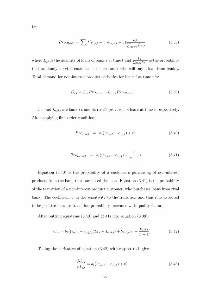
by:

ProiR→i,t =∑

f(eo,i,t − v, eo,i,R,t − v)Lj,t∑K 6=i LK,t

(3.38)

where Lj,t is the quantity of loans of bank j at time t andLj,t∑

K 6=i LK,tis the probability

that randomly selected customer is the customer who will buy a loan from bank j.

Total demand for non-interest product activities for bank i at time t is:

Oi,t = Li,tProi→i,t + Li,R,tProiR→i,t (3.39)

Li,t and Li,R,t are bank i ’s and its rival’s provision of loans at time t, respectively.

After applying first order condition:

Proi→i,t = b1((eo,i,t − eo,j,t) + v) (3.40)

ProiR→i,t = b1((eo,i,t − eo,j,t)−v

n− 1) (3.41)

Equation (3.40) is the probability of a customer’s purchasing of non-interest

products from the bank that purchased the loan. Equation (3.41) is the probability

of the transition of a non-interest product customer, who purchases loans from rival

bank. The coefficient b1 is the sensitivity to the transition and thus it is expected

to be positive because transition probability increases with quality factor.

After putting equations (3.40) and (3.41) into equation (3.39):

Oi,t = b1((eo,i,t − eo,j,t)(L1,t + Li,R,t) + b1v(Li,t −Li,R,tn− 1

) (3.42)

Taking the derivative of equation (3.42) with respect to L gives:

∂Oi,t

∂Li,t= b1((eo,i,t − eo,j,t) + v) (3.43)

86

Until now, v is assumed to be time independent. From now on, it is assumed to

be time dependent and bank-invariant and thus it is a function of the loanavity.

vt = v0 + b2Ht (3.44)

Now, v0 is the time independent switching cost. However, Ht is the time varying

loanavity factor. When long term loans increase, it is expected that banks can sell

non-interest products to their customers more easily. Then, putting equation (3.44)

into equation (3.43)

∂Oi,t

∂Li,t= b1((eo,i,t − eo,j,t) + v0 + b2Ht) (3.45)

Substituting the equation (3.45) into price-cost margin in equation (3.34) is given

by:

pcml,i,t = −b1v0Πo,t − b0gt+1n

n− 1δσl,i,t+1Ht −

σl,i,ta1

+ b1Πo,t(eo,i,t − eo,j,t)− b1b2Πo,tHt (3.45)

where Πo,t = (∂PoOt

∂Ot− ∂Ct

∂Ot)

Replacing S with St in equation (3.12), new loan market share equation is derived,

σl,i,t = e0 + a1(pl,i,t − pl,iR,t) + b0a1B + a1β0BHt (3.46)

where B = [ 1n−1− n

n−1σl,i,t−1]

3.4 Data

The sample consists of an unbalanced panel with annual observation from 2005

to 2012 for UK commercial banks. Investment, saving and cooperative banks are

excluded from the sample. All financial items are inflation adjusted to the base

year 2005 by using GDP deflator. Since theoretical model is valid for single market,

87

sample is determined for only one banking market: UK banking market. Even

European banking system created as an integrated market, it is difficult to assume

that banking system as a single banking system. Another advantage of the UK

banking system is that share of the non-interest income in total income is very high.

In 2005, share of the non-interest income in total income is 37%. For the year 2006,

its share decreases to the 28%, however, for the years 2010, 2011 and 2012, its shares

are 41% , 48% and 42%, respectively. Compared to European countries, these shares

are very high and it is an optimal country to analyse the pricing and switching

cost strategies associated with both traditional and non-traditional income side.

Thirdly, share of the public banks and mutual funds are also important in country

selection. These institutions may have different aims, such as social and development

objectives. Availability of non-profit aims is a barrier to clearly understand pricing

strategies that maximize bank profit. Henceforth, UK banking sector is a good

sample compared to other European countries.

Bankscope and other databases do not consist of maturity of deposit and loan

maturities. To assess loan diversification, new data is compiled including deposit

and loan maturities of individual banks from annual reports of each bank for 83

UK commercial banks. Some macroeconomic data are obtained from the World

Bank’s World Development Indicators (WDI). Because different banks have different

report styling, limitations of the bank number does not allow different maturity

measurements. Therefore, maturities are classified only as less than 1 year and

more than 1 year. Sample used in this analysis is less than the actual total number

of observations but highly representative, accounting for 83 percent of total banking

assets.

Some of the criteria reduce the number of total observations. Criteria imple-

mented in filtering are;

a) Missing years of dependent and independent variables were eliminated

b) Available abnormal returns or very large unexplained changes in the values of

any variables that distort the nature of the relationships were eliminated as outliers.

88

Mergers are dealt with as if they are composite bank for the entire period. However,

banks in exceptional conditions during the financial crisis are eliminated.

c) Available bank data less than 3 years in a row were eliminated for potential

econometric issues in calculation.

After the filtering, final dataset contains 555 observations.

3.5 Variables

The means and standard deviations of the variables used in this study are presented

at Appendix B. Models for price-cost margin and loan market share derived in the

theoretical part are as follows:

pcml,i,t = e0 − b0gt+1n

n− 1δσl,i,t+1Ht − b1v0Πo,t − a1σl,i,t

− b1Πo,t((eo,i,t − eo,j,t)− b1b2Πo,tHt

and

σl,i,t = e1 + a1(pl,i,t − pl,iR,t) + b0a1[1

n− 1− n

n− 1σl,i,t−1]

+ a1β0Ht[1

n− 1− n

n− 1σl,i,t−1]

3.5.1 Dependent Variables

Price - Cost Margin (PCM) : For price-cost margin in loan side, total interest

income minus total interest cost over total loan is introduced as the dependent

variable. Since price-cost margin reflects the profitability for the bank, interest

income minus interest expense reflects the price and cost for loan side.

In the theoretical part of this chapter, price-cost margin equation is derived that

equals the price of loan minus interest costs generated by loans. Therefore, price-cost

margin is tested in the empirical part. Interest rates charged by banks from the loan

89

activities and interest paid for these loan activities are not reported in the UK banks’

annual reports. In the unavailability of interest rates charged, total interest income

over the total loan is used and thus average interest rate is computed by each unit of

the loan. Similarly, in the absence of interest rates of deposits, interest expenditure

on each unit of loan is proxied by interest expense to loan ratio. Therefore, aligned

with the theoretical part of the third chapter, net interest income over total asset is

used to measure the price-cost margin of the banks.

Market Share (LOANSHARE) : Market share for loan is measured by loan of

each bank over total banking sector loans:

Loan share =yl,i,t∑ni=1 yl,i,t

where yl,i,t is the total loan of bank i at time t and∑ni=1 yl,i,t is the total loan in banking sector at time t, n is the number of banks

competing in that year. LOANSHARE is also an explanatory variable in the model

where price-cost margin is a dependent variable. Berger (1995) finds that firms

with higher market shares and differentiated products and services use this power

in pricing and earn higher profits.

3.5.2 Theoretical Explanatory Variables

Loan Price (LOANPRICE) : It shows the effect of loan price differences among

banks on the loan market share of the bank. It is measured by: pl,i,t − pl,j,R,t where

pl,j,R,t =∑

j 6=iwj,tpl,j,t is average rival price and wj,t =Lj,t∑ni=1 Li,t

is the share of each

rival bank in loan market.

Loan price of the current bank with respect to other rival banks may affect

customer decisions to stay at the same bank or switch to another bank. Theoret-

ically, loan price sensitivity of customers negatively impacts market share. Hence

parameter a1 is expected to be negative and takes values between 0 and -1.

BH : It is equal to [ 1n−1− n

n−1σl,i,t−1]Ht and it is the interaction of B and H. B is

measured by 1n−1− n

n−1σl,i,t−1. Ht is the long term loan to total loan that is a critical

variable to measure loanavity effect.

90

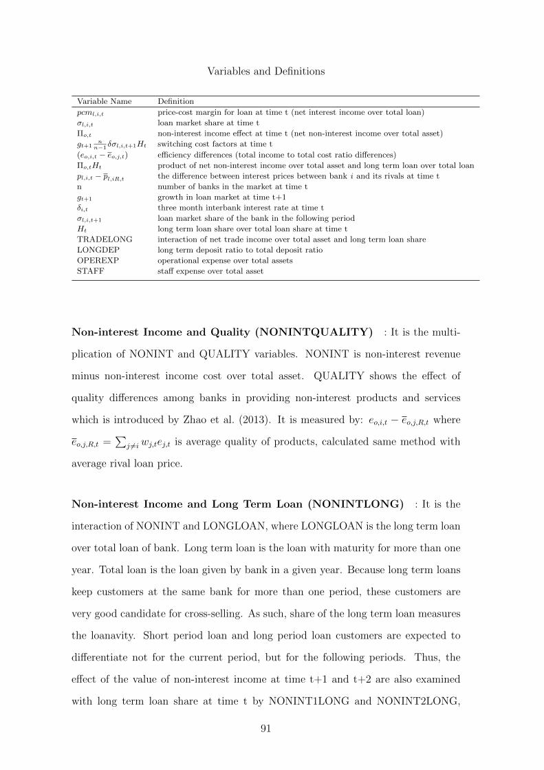
Variables and Definitions

Variable Name Definition

pcml,i,t price-cost margin for loan at time t (net interest income over total loan)

σl,i,t loan market share at time t

Πo,t non-interest income effect at time t (net non-interest income over total asset)

gt+1n

n−1δσl,i,t+1Ht switching cost factors at time t

(eo,i,t − eo,j,t) efficiency differences (total income to total cost ratio differences)

Πo,tHt product of net non-interest income over total asset and long term loan over total loan

pl,i,t − pl,iR,t the difference between interest prices between bank i and its rivals at time t

n number of banks in the market at time t

gt+1 growth in loan market at time t+1

δi,t three month interbank interest rate at time t

σl,i,t+1 loan market share of the bank in the following period

Ht long term loan share over total loan share at time t

TRADELONG interaction of net trade income over total asset and long term loan share

LONGDEP long term deposit ratio to total deposit ratio

OPEREXP operational expense over total assets

STAFF staff expense over total asset

Non-interest Income and Quality (NONINTQUALITY) : It is the multi-

plication of NONINT and QUALITY variables. NONINT is non-interest revenue

minus non-interest income cost over total asset. QUALITY shows the effect of

quality differences among banks in providing non-interest products and services

which is introduced by Zhao et al. (2013). It is measured by: eo,i,t − eo,j,R,t where

eo,j,R,t =∑

j 6=iwj,tej,t is average quality of products, calculated same method with

average rival loan price.

Non-interest Income and Long Term Loan (NONINTLONG) : It is the

interaction of NONINT and LONGLOAN, where LONGLOAN is the long term loan

over total loan of bank. Long term loan is the loan with maturity for more than one

year. Total loan is the loan given by bank in a given year. Because long term loans

keep customers at the same bank for more than one period, these customers are

very good candidate for cross-selling. As such, share of the long term loan measures

the loanavity. Short period loan and long period loan customers are expected to

differentiate not for the current period, but for the following periods. Thus, the

effect of the value of non-interest income at time t+1 and t+2 are also examined

with long term loan share at time t by NONINT1LONG and NONINT2LONG,

91

respectively. Value of loanavity is measured by b2 coefficient.

Switching Cost for Loan (SWITCH) : This variable measures the switching

cost for inter-temporal supply of loans. Different than other studies, now, vari-

able includes the effect of long term loans in switching cost. It is measured by

b0gt+1nn−1

δi,tσl,i,t+1Ht, where gt+1 is growth in loan market at time t+1, n is the

number of banks in the market for time t, δi,t is the three month interbank interest

rate at time t, σl,i,t+1 is the loan market share of the bank at time t+1 and Ht is

the long term loan share as long term loan over total loan at time t.

Trade Income and Long Term Loan (TRADELONG) : It is the interaction

of TRADE and LONGLOAN where TRADE is the trade revenue minus trade cost

over total asset. This variable is created to see whether long term particularly creates

a switching cost for trade products.

3.5.3 Non-theoretical Explanatory Variables

Share of Long Term Deposits (LONGDEP) : It is the ratio of long term

deposits over total deposits. Long term deposit is the deposit with maturity of more

than one year and total deposit is the sum of the short term and long term deposits.

Since short term and long term deposits have different magnitudes, changes in the

weights of maturities are tested. The coefficients d1 and d11 denote the effect of long

term deposits on price-cost margin and loan market share, respectively.

Operational Expense (OPEREXP) : Effect of the operational expenses on

price-cost margin is tested by operational expense over total asset of the bank. A

negative relationship between operational expense and price-cost margin is expected

due to the increase in costs.

Staff Expense (STAFF) : Staff expense, as one of the components of operational

expense, is also controlled, especially for the effect of it on loan market share. It

92

is reasonable to expect that an increase in staff expense improves the relationships

with current and potential customers and contributes to the bank by increasing

loan market share. As such increases in staff expenses may be positively linked with

market share.

For the years 2007, 2008 and 2009, time dummies are created due to the financial

crisis in the UK.

3.6 Methodology for Empirical Study

In this chapter, a system method is used: non-linear three stages least squares

(hereafter non-linear 3SLS). System estimating methods estimate all the structural

equations that identified in the system. Rather than separately estimating each

equation, system estimating procedure estimate equations together. Instead of us-

ing single equation method, by using systems method, all the available information

is evaluated in estimation procedures and thus, a relatively smaller asymptotic vari-

ance - covariance matrix is obtained (Kennedy, 2003). On the other hand, in the

availability of misspecification, all the structural parameters estimated in the sys-

tem are affected. In the single system, only the misspecified parameters are affected,

which is less costly.

Two of the system equations are 2SLS and 3SLS. 3SLS is the counterpart of the

2SLS. Each stages of 3SLS is as follows:

First Stage: Calculation of 2SLS estimates of the identified equations

Second Stage: By using the 2SLS estimates, errors of the structural equations are

estimated. These estimates are used to reach contemporaneous variance - covariance

matrix of the structural equations’ errors.

Third Stage: In the last stage, GLS is applied to the large equation representing

all the identified equations of the system.

One of the differences between 2SLS and 3SLS is that 2SLS, generally, is asymp-

totically less efficient than the 3SLS estimator. In this point, disturbances are the

main determinant of this difference. 3SLS makes same estimation if the disturbances

93

in the different structural equations are uncorrelated. In this case, the contempora-

neous variance - covariance matrix of the disturbances of the structural equations

is diagonal. In terms of consistency, the 3SLS estimator is a consistent estimator.

Because models in this study include non-linear parameters, this study uses a non-

linear 3SLS method. The variables and descriptive statistics are obtained by using

STATA program but due to using non-linear 3SLS method, the results were obtained

by SAS program.

3.7 Results

Table 3.2 displays the estimation results by using non-linear 3SLS for six specifica-

tions. The first model tests the theoretical foundations by using NONINTLONG

variable. The variable of NONINT1LONG, as the interaction of long-term loan

share at time t and non-interest income at time t+1, is tested in the second specifi-

cation. The third model replaces NONINT1LONG with NONINT2LONG. Effects

of non-theoretical variables, LONGDEP, OPEREXP and LABOR, are examined in

models four, five and six, respectively.

The coefficient a1 is a critical parameter for the theoretical model because it

shows the effect of price differences (a1 must take value within the [-1,0]). Table

3.3 demonstrate that a1 is negative and statistically significant. It takes values

higher than -1 by ranging between -0.067 and -0.084, which confirms the validity of

results and it is very close to the coefficients of Zhao et al. (2013). When the bank

loan price increases compared to the average rival loan price, customers choose to

switch to another bank. The negative value of coefficient a1 also implies that banks’

market share and loan price-cost margin are positively associated. The increase in

loan share is an indicator of market power. Banks use market power advantage by

increasing their prices.

Loan switching cost3 is tested by the coefficient b0. The positive sign of this

3This switching cost is very similar to switching cost suggested by Zhao et al. (2013). However,the current version includes the effect of Ht, which is the maturity effect as switching variable

94

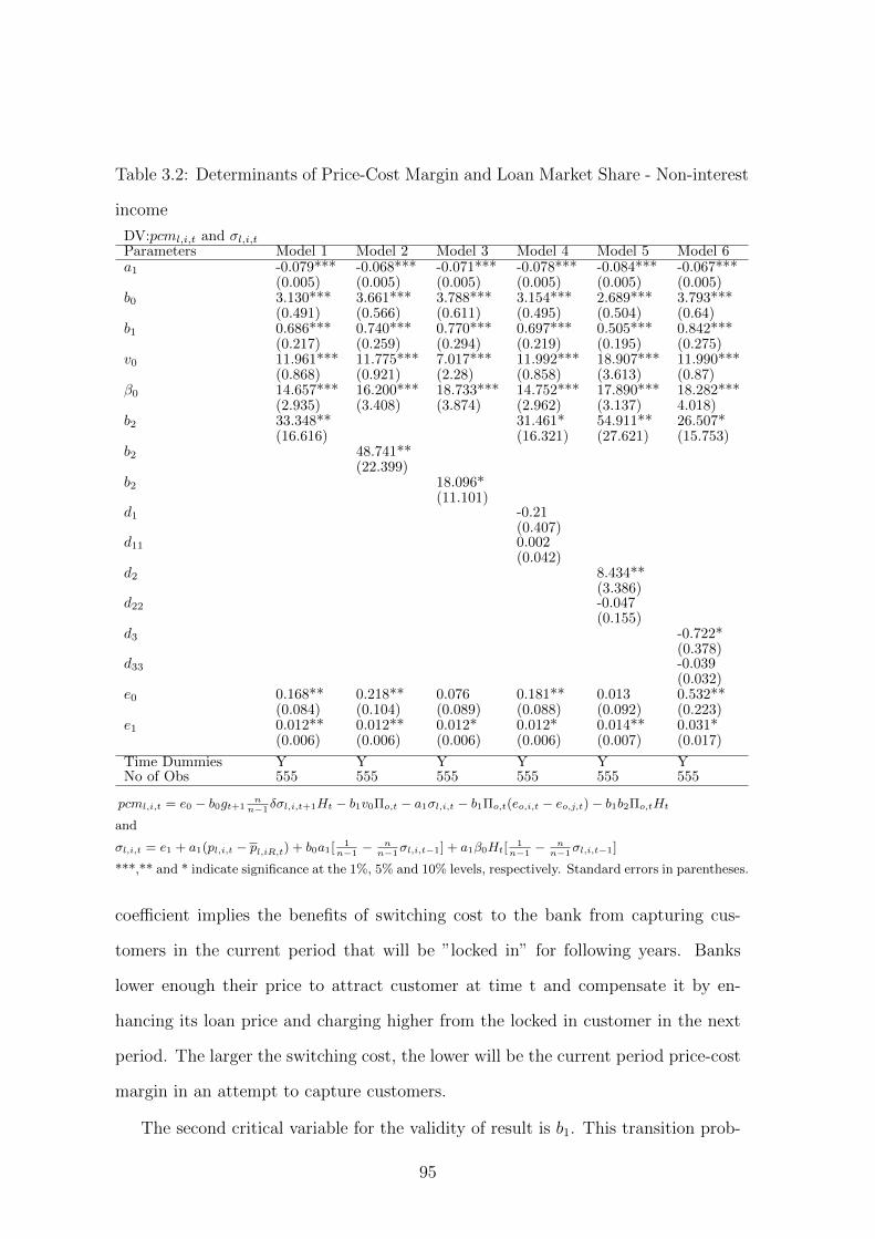
Table 3.2: Determinants of Price-Cost Margin and Loan Market Share - Non-interest

income

DV:pcml,i,t and σl,i,tParameters Model 1 Model 2 Model 3 Model 4 Model 5 Model 6a1 -0.079*** -0.068*** -0.071*** -0.078*** -0.084*** -0.067***

(0.005) (0.005) (0.005) (0.005) (0.005) (0.005)b0 3.130*** 3.661*** 3.788*** 3.154*** 2.689*** 3.793***

(0.491) (0.566) (0.611) (0.495) (0.504) (0.64)b1 0.686*** 0.740*** 0.770*** 0.697*** 0.505*** 0.842***

(0.217) (0.259) (0.294) (0.219) (0.195) (0.275)v0 11.961*** 11.775*** 7.017*** 11.992*** 18.907*** 11.990***

(0.868) (0.921) (2.28) (0.858) (3.613) (0.87)β0 14.657*** 16.200*** 18.733*** 14.752*** 17.890*** 18.282***

(2.935) (3.408) (3.874) (2.962) (3.137) 4.018)b2 33.348** 31.461* 54.911** 26.507*

(16.616) (16.321) (27.621) (15.753)b2 48.741**

(22.399)b2 18.096*

(11.101)d1 -0.21

(0.407)d11 0.002

(0.042)d2 8.434**

(3.386)d22 -0.047

(0.155)d3 -0.722*

(0.378)d33 -0.039

(0.032)e0 0.168** 0.218** 0.076 0.181** 0.013 0.532**

(0.084) (0.104) (0.089) (0.088) (0.092) (0.223)e1 0.012** 0.012** 0.012* 0.012* 0.014** 0.031*

(0.006) (0.006) (0.006) (0.006) (0.007) (0.017)

Time Dummies Y Y Y Y Y YNo of Obs 555 555 555 555 555 555

pcml,i,t = e0 − b0gt+1n

n−1δσl,i,t+1Ht − b1v0Πo,t − a1σl,i,t − b1Πo,t(eo,i,t − eo,j,t) − b1b2Πo,tHt

and

σl,i,t = e1 + a1(pl,i,t − pl,iR,t) + b0a1[ 1n−1

− nn−1

σl,i,t−1] + a1β0Ht[1

n−1− n

n−1σl,i,t−1]

***,** and * indicate significance at the 1%, 5% and 10% levels, respectively. Standard errors in parentheses.

coefficient implies the benefits of switching cost to the bank from capturing cus-

tomers in the current period that will be ”locked in” for following years. Banks

lower enough their price to attract customer at time t and compensate it by en-

hancing its loan price and charging higher from the locked in customer in the next

period. The larger the switching cost, the lower will be the current period price-cost

margin in an attempt to capture customers.

The second critical variable for the validity of result is b1. This transition prob-

95

ability for the non-interest product is expected to be positive, but it must be lower

than 1. Values lower than 0 imply the transition of customers due to the higher

quality of services that they left, which is implausible. The significant and positive

value of b1 states that quality differences and switching cost associated from loanav-

ity contribute to the switching cost and, therefore, customer’s willingness to switch

to other banks for non-interest product and service decreases.

Another theoretical coefficient v0 is also statistically significant. v0 > 0 states

that time invariant incompatibility cost is positive. Switching is costly for customers

due to the compatibility issue, transaction cost related to closing and opening ac-

counts, new brand adaptation costs and uncertainty about the quality (Klemperer,

1995). Brehm (1956) also points out the social psychology in favour of the previ-

ously used products. Another theoretical coefficient β0 is also statistically significant

and positively associated with loan market share as it is expected from theoretical

derivation.

b2 theoretically represents switching cost for non-interest products and services

stems from having a long-term loan. According to the results, it is positive and

statistically significant. This result confirms that increasing the share of the long-

term loan in total loan contributes to bank creating a switching cost for non-interest

products and services. First, this may be related to improvements in the relation-

ship by the loan. Banks can use personal information of customers to persuade them

to purchase non-interest product or services. Banks may also use communication

devices properly to reach customer particularly modelling the customer needs. Sec-

ond, there is an information asymmetry between the inside- and outside bank that

changes the likelihood of rejection. A customer who has long-term loan contract

with a bank may feel that likelihood of rejection for a non-traditional product is

higher for outside banks. Third, during the maturity of the long-term loan, the

customer may have inertia to buy non-interest products and services from the same

bank thanks to the long-term loan. Fourth, the long-term loans require, by its very

nature, many complement products especially during the application period such as

96

Table 3.3: Determinants of Price-Cost Margin and Loan Mar-

ket Share - trade income

DV:pcml,i,t and σl,i,tParameters Model 1 Model 2 Model 3

aa1 -0.076*** -0.080*** -0.079***(0.005) (0.005) (0.005)

bb0 3.181*** 2.967*** 3.198***(0.483) (0.467) (0.476)

bb1 0.781*** 0.710*** 0.666***(0.225) (0.218) (0.231)

vv0 3.397 8.726 11.586*(7.02) (6.01) (6.6)

ββ0 15.588*** 15.701*** 14.500***(2.942) (2.903) (2.864)

bb2 30.830*(19.208)

bb2 25.888*(15.549)

bb2 17.769(13.953)

ee0 0.012 0.023 0.018(0.07) (0.069) (0.071)

ee1 0.012 0.012** 0.012**(0.006) (0.006) (0.006)

Time Dummies Y Y YNo of Obs 555 555 555

pcml,i,t = ee0−bb0gt+1n

n−1δσl,i,t+1Ht−bb1v0Πo,t−aa1σl, i, t−bb1Πo,t(eo,i,t−

eo,j,t) − bb1bb2Πo,tHt

and

σl,i,t = ee1 + aa1(pl,i,t − pl,iR,t) + bb0aa1[ 1n−1

− nn−1

σl,i,t−1] + aa1β0Ht[1

n−1−

nn−1

σl,i,t−1]

***,** and * indicate significance at the 1%, 5% and 10% levels, respectively.

Standard errors in parentheses.

non-traditional income activities ( e.g. the application of long-term housing credits).

Some of these non-interest income activities are inseparable, and some of them are

highly complementary. The necessity for compliments of long-term loan tends to

provide the customer of the same bank by good offers (e.g. bundling which creates

time and research cost for the customer). A bank reduces the price of the long-term

loan and then offset it today or in the future by selling non-interest products and

services from higher price to lock the customer in. The significant value of b2 in

97

models 2, and 3 also imply that an increase in loan’s maturity at time t lowers

the price-cost margin conditional on non-interest income at time t + 1 and t + 2,

respectively. Thus, a positive and significant values of b2 confirm the theoretical

foundation associated with loanavity.

d1 denotes the effect of the long-term share of the total deposits is also insignifi-

cant implying that shifting from short-term to the long-term deposits, surprisingly,

has no explanatory power in explaining the price-cost margin. Deposits are assumed

to be cheaper than outside funding and hence expected to raise the price-cost mar-

gin by lowering the costs of the bank. Moreover, another coefficient of LONGDEP,

d11, also insignificant to explain banks’ loan market share.

The effect of the OPEREXP is tested by d2 and d22. The results state that

operational expenses are positively linked with the price-cost margin for the UK

banking system. This relationship implies that an increase in operational costs

increases the price-cost margin by probably increasing the price. The negative sign

of d22 states that operational cost reduces the market share of the bank. However, it

is statistically insignificant to explain market share. Model 6 in Table 3.2 examines

the effect of staff cost. Interestingly, different than d2, d3 is negatively associated

with price-cost margin but d33 is insignificant, like d22. This difference implies that

operational cost except labour cost help banks to increase their price-cost margin.

Probably these expenditures contribute more to the value added.

Table 3.3 depicts the effect of switching cost of long-term loan conditional on

trade income. Testing the effect of long-term loans conditional on trade products

and services also proved to be valuable for the analysis. The result shows that long-

term loans create a switching cost for trade products and service. The switching

cost effect of long-term loan for trade income is statistically significant at time t and

t+ 1 but statistically insignificant at time t+ 2.

98

3.8 Conclusion

This study theoretically extends Kim et al. (2003)’s switching cost model by incor-

porating the loan maturity as a switching cost factor for non-traditional products.

The study empirically examines this theoretical contribution for the UK banking

system by using unique banking data compiled by the author. The empirical results

show that shifting from short-term to long-term loans increases the switching cost

for non-traditional products. Banks lower their long-term loan price to start creating

this switching cost. Banks use the personal information of customers to persuade

them to purchase non-interest products or services through the improvements in

the relationship using long-term loans. A customer who has a long contract with a

bank may feel that the likelihood of rejection of a non-traditional product is higher

for outside banks, due to information asymmetry. The relationship between the

customer and the bank strengthens as a result of the long-term loan and this may

create an inertia, which in turn increases along with the maturity of the loan con-

tract, to buy a non-interest products from the same bank. Compared to short-term

loans, long-term loans characteristically require many complementary products, par-

ticularly during the application period. The necessity for complementary product

augments for long- term loan customers, thus the bank provides him good offers

(e.g. bundling) which creates time and research costs for the customer.

The empirical results indicate that this situation is valid for trade products, as

well. The relationship between trade income and maturity is significant as expected.

When loanavity increases, customers switch to trade products. Banks decrease the

loan price to a level sufficient enough to attract long-term customer, this locking the

customers in. Such act gives them a chance to sell them trade or other non-interest

products and services in the subsequent periods.

Similar to prior literature, the study finds that loan price and market share

are negatively associated. Customers prefer to switch in response to an increase

of loan price, relative to average loan price of rival banks. The price-cost margin

is also positively related to loan market share. The increase in market share, as

99

an increase in market power, increases the price of the loan and hence increases

price-cost margin.

This study also introduces the deposit maturity, as a non-theoretical variable,

to test its effects on price-cost margin and loan market share. The results state

that increase in long-term deposits has no explanation power to explain for neither

price-cost margin nor loan market share.

The study also controls for some other non-theoretical variables. The results

indicate that operational expenses increase the price-cost margin while staff expenses

decrease the price-cost margin. These variables have no explanatory power for loan

market share.

Most of the studies in the literature find that cross-selling may create a risk for

banks. The increasing covariance between interest and non-interest income sides by

cross-selling amplify the bank’s risk in the face of the unexpected income shocks.

Regulators should consider the correlation level between these two sides. In particu-

lar, they should carefully understand the strategies of banks. This study result helps

banks, supervisors and regulators to consider the switching cost effect on shifting

from short-term to long-term loans for non-traditional products. Second, long-term

loans, are one of the best candidates to compensate loss from lock the customer in

through non-interest products. High level of complementarity and time are two key

advantages of long-term loans. Banks that are mostly interested in switching cost,

should give more importance to the switching cost effect of long-term loans, without

ignoring the risk which stems from cross-selling.

This study theoretically implements a linear relationship between transition

probability and switching cost. Further studies may contribute to the literature

by considering a non-linear relationship. Further studies should also test the effects

of long-term deposits as a switching cost factor. Loans require complementary prod-

ucts and it is reasonable to create a switching cost for them. However, as mentioned

above, potential inertia can be created by increasing deposit maturity or from banks

gathering more information about their customers as the maturity of deposits in-

100

crease. This information is used to persuade the customer to buy the non-interest

products. Potential switching costs created by deposits may impact profitability

and risk, too. Lastly, this study considers the loan customers as short and long term

customers, due to the barriers associated with lack of detailed data. Further studies

may analyse the duration by details, for example, considering at least three terms:

short, medium and long term. Finally, the results help banks and regulators to see

the evolution of switching costs more clearly.

101

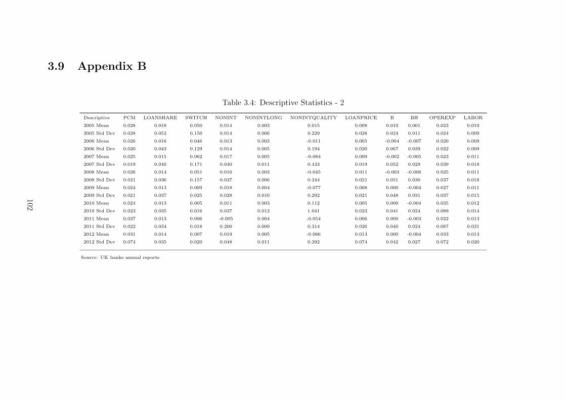
3.9 Appendix B

Table 3.4: Descriptive Statistics - 2

Descriptive PCM LOANSHARE SWITCH NONINT NONINTLONG NONINTQUALITY LOANPRICE B BH OPEREXP LABOR

2005 Mean 0.028 0.018 0.050 0.014 0.003 0.015 0.008 0.010 0.001 0.023 0.010

2005 Std Dev 0.028 0.052 0.150 0.014 0.006 0.229 0.028 0.024 0.011 0.024 0.009

2006 Mean 0.026 0.016 0.046 0.013 0.003 -0.011 0.005 -0.004 -0.007 0.020 0.009

2006 Std Dev 0.020 0.043 0.129 0.014 0.005 0.194 0.020 0.067 0.039 0.022 0.009

2007 Mean 0.025 0.015 0.062 0.017 0.005 -0.084 0.009 -0.002 -0.005 0.023 0.011

2007 Std Dev 0.019 0.040 0.171 0.040 0.011 0.433 0.019 0.052 0.029 0.039 0.018

2008 Mean 0.026 0.014 0.051 0.016 0.003 -0.045 0.011 -0.003 -0.006 0.025 0.011

2008 Std Dev 0.021 0.036 0.157 0.037 0.006 0.244 0.021 0.051 0.030 0.037 0.018

2009 Mean 0.024 0.013 0.009 0.018 0.004 -0.077 0.008 0.000 -0.004 0.027 0.011

2009 Std Dev 0.021 0.037 0.025 0.028 0.010 0.292 0.021 0.048 0.031 0.037 0.015

2010 Mean 0.024 0.013 0.005 0.011 0.003 0.112 0.005 0.000 -0.004 0.035 0.012

2010 Std Dev 0.023 0.035 0.016 0.037 0.012 1.041 0.023 0.041 0.024 0.089 0.014

2011 Mean 0.027 0.013 0.006 -0.005 0.004 -0.054 0.006 0.000 -0.003 0.022 0.013

2011 Std Dev 0.022 0.034 0.018 0.200 0.009 0.314 0.026 0.040 0.024 0.087 0.021

2012 Mean 0.031 0.014 0.007 0.019 0.005 -0.066 0.013 0.000 -0.004 0.033 0.013

2012 Std Dev 0.074 0.035 0.020 0.048 0.011 0.392 0.074 0.042 0.027 0.072 0.020

Source: UK banks annual reports

102

Chapter 4

Bank Performance Effect of

Deposit and Loan Maturities

Abstract

This study examines the effect of non-interest income, conditional on deposit and

loan maturities, on bank performance using unique data on the United Kingdom

(UK) banks during the period 2005 - 2012. It is the first study to examine the di-

rect maturity effect of both deposits and loans, as short term and long term, on bank

performance for UK banks. The findings suggest that fees and commission income

do not directly explain banks’ performance. However, when the fees and commission

variable is conditional on longer loan maturities, it reduces the bank performance.

Trade income increases the risk-adjusted bank performance, but trade income, con-

ditional on longer deposit and loan maturities, has the opposite effect. The direct

diversification results reveal that maturity diversification of loans is associated with

higher bank performance, whilst the UK banks do not benefit from deposit diversifi-

cation. The framework, adopted in this study aims to help banks pay more attention

to deposit diversification rather than focusing on both sides. The results also provide

significant implications for regulators and supervisors in the UK, as well as other

developed countries, to consider the direct and indirect effects of the maturities on

bank performance.

103

4.1 Introduction

Competition, technological advances and regulatory pressure among others are fac-

tors that led banks to diversify their operations from traditional lending only to

the inclusion of non-interest bearing activities as well. The implication of this shift

towards generating non-interest income activities had a significant effect on banks’

performance. Pursuing the maximisation of shareholders wealth, banks initiate new

policies and innovate to sell non-interest products to either current or potential

customers. The process of selling non-interest products to the present and new

customers is known in the literature by cross-selling. However, even persuading cur-

rent customers (depositor or borrowers) to buy a non-interest product may require

time. This time is directly linked to the maturities of interest products in the sense

that the longer the maturities of both deposits and loans, the shorter the time to

persuade the customer; catalyst role. In this vein, long-term customers are of great

importance for banks to be able to sell non-traditional products. Banks continuously

improve communication means and learn more about that borrower’s characteris-

tics to reduce information asymmetry (Kane and Malkiel, 1965; Fama, 1985). They

introduce new technologies to build closer relationships with customers in order to

identify customers’ product preferences; understand their lifestyle and spending pat-

terns; and their demand for other services. Every transaction in the past enriches

the information about customers and increases the predictive power of the future.

Gathered information may be used in multiple interactions with the same customer

and create a chance to benefit from inter-temporal reusability (Greenbaum et al.,

2015). This proprietary information creates ex-post monopoly power for banks to

sell non-interest products. Moreover, with respect to loan size, one of the distinctive

characteristics of long-term maturity is that size of the loan increases in maturities.

The increase in loan size may require, by its very nature, more fee and commission

transactions. The overall conclusion is that an increase in maturity is expected to

pave the way for selling non-traditional products to core customers.

The empirical literature questions the benefit from the cross-selling policy adopted

104

by banks. A common finding is that the cross-selling policy of banks is one of the

drawbacks that may have detrimental effect on the diversification policies (Boyd

and Graham, 1986; Lown et al., 2004; Stiroh, 2004; Lepetit et al., 2008). Excessive

cross-selling by a bank may lead to the augmentation of customer’s debt which is

positively associated with bank’s risk. Furthermore, the occurrence of an income

shock to the customer will hinder her ability to pay the charges for both traditional

and non-traditional products thus exposing the bank to performance fragility. On

the benefits side, cross-selling assists banks to decrease information asymmetry and

thus acts as a barrier to moral hazard problems. Banks can easily score the perfor-

mance of their customers and can be more selective in their cross-selling policy to

long-term customers.

The preceding discussion shows that cross-selling is directly associated with ma-

turity either in the assets (loans) or liabilities (deposits) sides of banks’ balance

sheets. Therefore the issue of maturity naturally positions itself as a corner stone

in this study. Banks need to diversify their assets and liabilities in terms of their

maturity for various reasons (such as for meeting customers’ demands, managing

liquidity or reducing capital requirements). However, income and product diversi-

fication strategies may conflict with the maturity diversification strategies creating

a maturity mismatch that in turn may affect banks’ performance. The maturity

mismatch between deposits and loans, in some conditions, may cause illiquidity

and insolvency to banks. Therefore, banks are expected to mitigate liquidity risk

by adopting true maturity diversification policy. There is an increasing role of

non-interest income in banks operation given their relatively new experience to the

pricing strategies by banks. In particular, the role it plays for long-term customers.

In this context, a profit maximizer bank may not necessarily know or calculate the

optimal risk and return strategies. The banking sector in the UK has less regional,

state, co-operative or mutual banks that are likely not to have profit maximizing

pricing and cross-selling strategies. During the period 2007 - 2012 the UK banks

were heavily reliant on non-interest income (around 38.0% of total income). There-

105

fore it is important to examine the cross-selling policies of the UK banks and their

effect on performance.

This study addresses an important gap in the literature by investigating the

effect of cross-selling strategies on banks’ performance conditional on deposit and

loan maturity. The shift towards long-term deposits and loans may increase cross-

selling and hence contribute to higher levels of bank revenue. The increase in revenue

may be accompanied by higher volatility of income and increased risk. The potential

hazard is caused by the longer maturity of deposits and loans critical for banks and

regulators that should focus on bank risk factors. The scarcity of detailed data about

loans and deposits maturities acted as a fence for researchers to test the direct and

indirect impacts of maturity on banks performance.

The study contributes to the literature in two folds. First, it provides important

evidence to the existing banking diversification-performance literature by consider-

ing the indirect effect of deposit and loan maturities on banks performance. This

strand is mainly focused on income and geographical diversification. The study uses

a unique data on the United Kingdom(UK) banks from 2005 to 2012. In addition,

the study provides valuable insight into the link between cross-selling, conditional on

the degree of maturity, and bank risk. The results reveal that fees and commission

income do not explain banks’ performance in a direct form. On the other hand, the

fees and commission variable conditional on long-term loan maturity reduces the

bank performance. The trade income increases the risk-adjusted bank performance,

but trade income conditional on longer maturity has the opposite effect. Second, to

our knowledge, this is the first study to examine the direct effect of maturity of both

deposits and loans on bank performance. The study departs from the traditional ap-

proach of direct matching of deposits and loans and separately measures the effect of

maturities of deposits and loans. This approach allows detecting the separate matu-

rity effects of deposits and loans on banks performance. The results indicate that the

maturity diversification of loan is associated with higher bank performance. How-

ever, UK banks do not benefit from deposit diversification. Different explanations

106

of the power of the deposit and loan diversification implies that compared to loan

diversification, banks should pay deposit diversification more attention, possibly due

to the optimality of loan diversification by alternative funding channels. The study

use System GMM method to count for endogeneity and unobserved heterogeneity in

the sample. For robustness purposes, three alternative indicators were used as prox-

ies for risk namely Z-score, risk-adjusted return on assets and risk-adjusted return

on equity.

The rest of the chapter unfolds as follows: Section 4.2 is comprised of the lit-

erature review on bank performance, diversification and funding to understand the

concepts and their effects. Section 4.3 presents the portfolio theory associated with

diversification and risk. Section 4.4 defines and explains the dependent and inde-

pendent variables used in our analysis. Section 4.5 describes the data and presents

the econometric method employed in the study. Section 4.6 is the discussion of the

results. Section 4.7 concludes.

4.2 Literature Review

There is abundant evidence in the literature on the benefits of diversification in

reducing banks’ risks. Some of these studies even suggest that apart from reducing

bank’s risk diversification may help in improving managerial skills. Nonetheless,

the literature on bank diversification recently presents mixed results. The recent

evidence from the literature is contesting the theoretical underpinning of portfolio

theory regarding the benefits of diversifications.

Boyd and Graham (1986) and Boyd et al. (1993) test the riskiness of hypothetical

mergers between bank holding companies and non-bank financial companies. The

findings suggest that mergers between bank holding companies and life insurance

firms reduce the risk of bankruptcy. Saunders and Walter (1994) state that being

open to new activities enables banks to reduce their risk. Cybo-Ottone and Murgia

(2000) analyse the effect of Merger and Acquisitions (M&A) on returns in European

banking for the period 1988 and 1997. They find that M&A create positive abnormal

107

returns, due to the product diversification. On the other hand, they also find that

M&A with securities firms and foreign institutions did not generate any gain. From

income diversification perspective, Wall and Eisenbeis (1984) find that diversifying

into non-interest activities help banks to reduce their risk. Gallo et al. (1996) test

the riskiness of bank holding companies and effects of mutual fund activities on

bank risk and profitability. They find that mutual fund activities reduce banks’

exposure to the industry risk. However, these activities are modest to reduce bank

unsystematic risk. They also find that bank profitability is positively associated

with increased mutual funds activities.

Deng and Elyasiani (2008) imply that geographic diversification contributes to

banks’ value maximization and decreases total risk. They show that the distance

between bank holding companies and their branches is inversely related to firm value

and directly linked to risk. Hughes et al. (1999) find that efficiency improves thanks

to geographical diversification while growth in product and geographic diversifica-

tion reduces the bank risk. Another view argues that global diversification does not

affect operating performance negatively, which implies that the idea of misallocation

of resources by global diversification is not accurate (Iskandar-Datta and McLaugh-

lin, 2005). According to the authors, leveraging managerial skills and abilities for

the products and geographic region are the significant benefits of diversification. In

contrast, Morgan and Samolyk (2003) test the geographic diversification and find

that diversification does not improve loan performance or returns. Diversification

helps banks to increase their lending capacity resulting in a higher loan to asset

ratio. However higher loan to asset ratio does not increase profit or reduce risk.

Some other studies state that income diversification causes a minor scale economy

effect (Lawrence, 1989; Ashton, 1998; Humphrey, 1990). Drucker and Puri (2009)

note that banks benefit from economies of scope by selling non-interest income with

the same fixed costs in traditional activities. Boot and Schmeits (2000) suggest that

diversified financial institutions may reduce the expected costs which stem from fi-

nancial distress or bankruptcy conditional on spreading operations across different

108

products. The literature also provides evidence on the adverse effects of diversifi-

cation. Boyd and Graham (1986) and Lown et al. (2004) find that the increasing

trend towards non-bank activities raised the risk of the failure of banks during the

seventies. They investigate bank mergers across the financial services industries;

their findings show that the combination of bank holding and life insurance compa-

nies augments diversification benefit. However, mergers between securities, property

insurance, and casualty insurance firms are likely to increase the bank holding com-

panies’ risk albeit to a limited extent. Rosen et al. (1989) examine the diversification

benefits for 319 banks involved in real estate activities from 1980 to 1985 and find

that diversification towards real estate activities has a modest effect on banks’ risk.

However, the positive correlation between returns is overwhelmed by the greater

deviations of real estate returns.

Templeton and Severiens (1992) examine the effects of activity diversification for

54 bank holding companies by using market-based data and find that diversification

leads to a lower variance of shareholder returns but has no explanation power for

systematic risk. Kwast (1989) aims to explain the benefits of existing underwriting

and dealing activities to bank returns and risk. His study indicates limited gains

from diversification. Kwan (1998) tests the contribution of existing banking and

securities activities on bank profitability and risk for the period 1990 - 1997 using

micro data of banks’ securities affiliates. He finds that securities trading tends to

be riskier but also more profitable, however the proliferation of risk stems from

their higher leverage. DeYoung and Roland (2001) analyse data from 472 large and

medium sized commercial banks covering the period from 1988 to 1995. Their prime

aim is to examine the relationship between earning volatility and fee-based activi-

ties. Their result suggests that income diversification generates a new revenue line

for banks but equally adds new business risks. The fee-based activities are positively

correlated with earning volatility, implying that when banks shift their income ac-

tivities from interest based activities to fee-based activities, their earnings become

more volatile. Thus shifting to fee-based activities increases the risk associated with

109

income diversification. Authors attributes this situation to costs in shifting from

one bank to another. According to the authors, banks bear switching and informa-

tion costs by shifting banks’ activities from lending relationship to fee-based. These

costs are switching and information cost. The volatility of the interest revenue is

rather stable compared to the fee-based income. However, the latter requires limited

bank-customer relationship and henceforth it is less costly and more volatile.

Acharya et al. (2002a) examine the effects of specialization versus diversification

on bank risk and return by using the data of 105 Italian banks for the period 1993

- 1999. The result shows that diversification of bank assets neither improve nor

reduce bank risk.

Stiroh (2004) examines the effects of non-interest income components on diver-

sification benefits during the period 1984 - 2001 in the US banking industry. The

results indicate that the shifting to non-interest income by diversification increases

the bank risk and decreases the risk-adjusted performance indicators. Such relation-

ship is caused by the high correlation between the non-interest income and trade

income which led to higher volatility. The study also detects a higher correlation

between the growth rates of interest income and non-interest income during the

1990’s, compared to the 1980’s. The study does not test directly bundling strategies

or fee policy but because of decreasing risk-adjusted bank performance and increas-

ing the covariance between interest and non-interest income, the author states that

cross-selling may have increased in this period thus implying the adverse effect of

potential shocks in decreasing bank performance.

Stiroh and Rumble (2006) investigate the impact of non-interest income on the

performance of US financial holding companies over the period 1997 - 2002. They

find that shifts to the non-interest activities are inversely related with risk-adjusted

bank performance. Moreover, the costs associated with the high volatility of non-

interest income offsets the benefits from diversification. This result implies that

banks cannot attain optimal benefits from their diversification policy. The authors

suggest that the problem may be related with misunderstanding of diversification

110

concept. They elaborate that if the main idea behind diversification is cross-selling to

reduce costs and increase profit, then, they may ignore the potential risks associated

with potential shocks to the same customer. Another possible factor explained by

the author is the priorities of the bank management if they are large equity holders.

The bank management may give priority to profit maximization and less attention to

the income volatility. The third explanation about the adversity of diversification

is the overreaction to the lending problems in earlier periods. In order to avoid

lending issues, the financial holding companies may push themselves towards new

non-interest income activities. Their final explanation is that the study may have

covered the incorrect period to analyse diversification benefits but also suggest that

similar results are valid for older periods which in turn reduces the likelihood of the

problem in that time.

Mercieca et al. (2007) analyse the effect of income diversification on bank perfor-

mance for small European banks using in 15 countries from 1997 to 2003. Their sam-

ple includes 755 credit institutions with asset size less than 450 million Euros. The

study employs the Z-score, the risk-adjusted return on asset and the risk-adjusted

return on equity as three alternative proxies for bank insolvency risk. They find

that there are no direct diversification benefits for small European banks. The re-

sult shows that non-interest income is inversely linked to risk-adjusted performance

suggesting that small financial institutions are better at specializing and diversifica-

tion benefits are not valid for these institutions. Lepetit et al. (2008) examine the

association between bank diversification and the European banking industry over

the period 1996 and 2002. Their results show that banks which shifts to non-interest

income activities from traditional loan activities have poorer performance and have

higher insolvency risk. The authors report that the default risk is inversely related

to trading activities but positively associated with a larger share of fee-based activ-

ities for small banks. However, fee- or trading based activities provide insignificant

to risk for large banks.

111

Berger et al. (2010) examine the benefits of diversification for Chinese banking

systems using data for the period 1996 - 2006. Considering loans, deposits, assets

and geography diversifications, the authors measure the performance of Chinese

banking system, as a developing country banking system. The results indicate that,

after controlling for risk, diversification increases the costs and decreases profits for

these four dimensions. Zhou (2014) measures the impacts of income diversification

on bank risk for 62 Chinese commercial banks over the period 1997 - 2012. The

author finds that there is no statistically significant relationship between income

diversification and bank risk. While non-interest income increases the risk because

of high volatility, traditional interest income activity contributes to the decrease in

risk.

Demirguc-Kunt and Huizinga (2010) find that bank’s rate of return and its risk

increase with higher proportions of fee income. The study investigates a sample

of 1,334 banks in 101 countries, from 1995 to 2007. Their result suggests that fee

incomes may produce risk diversification benefits however at very low levels while

the wholesale funding lowers the rate of return on assets. They also claim that the

reactions of depositors and wholesale funders are different. The wholesale funders

quickly react to bank’s risk performance. Huang and Ratnovski (2011) provide a

model that investigates banks reliance on wholesale funding. They argue that banks

that generate cheap and noisy signals may provide the wholesale financiers with in-

centives to withdraw their funding. Myers and Rajan (1995) point the differences

in asset mix. They claim that banks cannot optimally benefit from income diversi-

fication. However, they are likely to diversify their income to obtain more liquidity

from non-traditional banking activities. Song and Thakor (2007) suggest that re-

lationship loans which stem from opaqueness are financed by core deposits since

liability holders can’t easily evaluate bank solvency. The probability for depositors

to withdraw their funds prematurely as a precaution is relatively low.

In consideration of other different diversification policies, Jr and Nash (1993)

explain the riskiness and profitability of institutions specialized in credit card loans

112

over the period 1984 and 1991. The authors find that banks specialized in credit

cards obtain positive abnormal returns compared to those with traditional product

mixes. However, their likelihood of insolvency increases due to the increase in return

on assets volatility. Similarly, Lang and Stulz (1993) find that the value of diversified

firms is less than the specialized firms. Rose (1989) highlights the amplification in

cash flow risk when banks shift towards non-bank product lines. Denis et al. (1997)

also suggest that financial institutions should keep their firms in a single line of

business rather than diversification because of the agency cost. They find that

managerial equity ownership is negatively associated with diversification and reduce

agency cost. Acharya et al. (2002b) argue that expanding into other industries

and sectors creates issues of weakened monitoring quality for risky banks. Another

problem is the quality of the loan portfolio for these risky banks. They also suggest

that industrial loan diversification lessens bank return.

4.3 Portfolio Theory

The trade-off between risk and return is a long-standing predicament for banks.

The microeconomic theory depicts this relationship in the portfolio theory (Sharpe,

1964). The theory assumes that the outcome of any investment is calculated by

probabilistic values. The potential outcome is calculated by the sum of possible

outcomes and their probabilities. If the outcomes involve risk, the investor chooses

among possible outcomes to derive the highest level of utility. In the same spirit,

Stiroh (2004) investigates bank’s income volatility, by considering the proportion of

interest income on the total income as α for the output INT and the percentage of

non-interest income to total income as (1−α) for the output NONINT. Accordingly

the expected return (ER) is

ER = αINT + (1− α)NONINT (4.1)

113

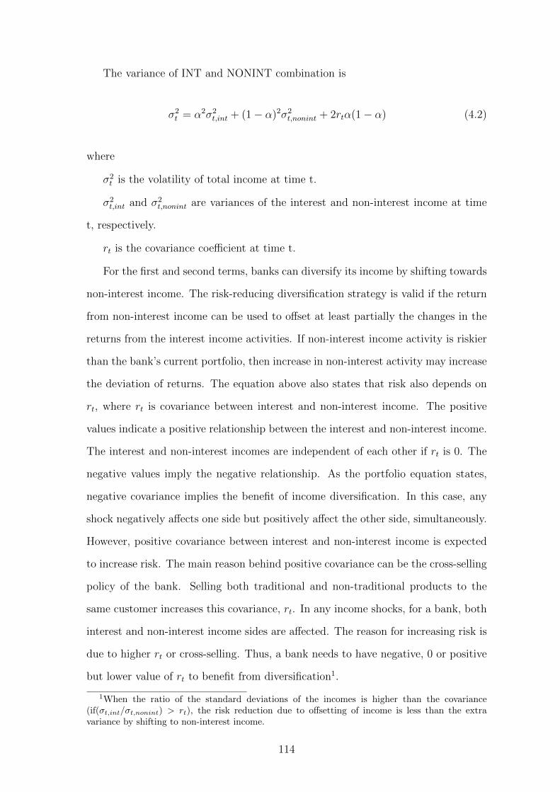
The variance of INT and NONINT combination is

σ2t = α2σ2

t,int + (1− α)2σ2t,nonint + 2rtα(1− α) (4.2)

where

σ2t is the volatility of total income at time t.

σ2t,int and σ2

t,nonint are variances of the interest and non-interest income at time

t, respectively.

rt is the covariance coefficient at time t.

For the first and second terms, banks can diversify its income by shifting towards

non-interest income. The risk-reducing diversification strategy is valid if the return

from non-interest income can be used to offset at least partially the changes in the

returns from the interest income activities. If non-interest income activity is riskier

than the bank’s current portfolio, then increase in non-interest activity may increase

the deviation of returns. The equation above also states that risk also depends on

rt, where rt is covariance between interest and non-interest income. The positive

values indicate a positive relationship between the interest and non-interest income.

The interest and non-interest incomes are independent of each other if rt is 0. The

negative values imply the negative relationship. As the portfolio equation states,

negative covariance implies the benefit of income diversification. In this case, any

shock negatively affects one side but positively affect the other side, simultaneously.

However, positive covariance between interest and non-interest income is expected

to increase risk. The main reason behind positive covariance can be the cross-selling

policy of the bank. Selling both traditional and non-traditional products to the

same customer increases this covariance, rt. In any income shocks, for a bank, both

interest and non-interest income sides are affected. The reason for increasing risk is

due to higher rt or cross-selling. Thus, a bank needs to have negative, 0 or positive

but lower value of rt to benefit from diversification1.

1When the ratio of the standard deviations of the incomes is higher than the covariance(if(σt,int/σt,nonint) > rt), the risk reduction due to offsetting of income is less than the extravariance by shifting to non-interest income.

114

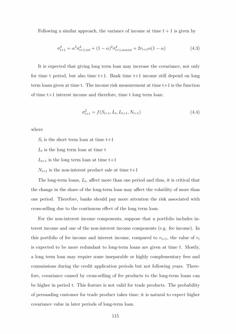
Following a similar approach, the variance of income at time t+ 1 is given by

σ2t+1 = α2σ2

t+1,int + (1− α)2σ2t+1,nonint + 2rt+1α(1− α) (4.3)

It is expected that giving long term loan may increase the covariance, not only

for time t period, but also time t+1. Bank time t+1 income still depend on long

term loans given at time t. The income risk measurement at time t+1 is the function

of time t+1 interest income and therefore, time t long term loan:

σ2t+1 = f(St+1, Lt, Lt+1, Nt+1) (4.4)

where

St is the short term loan at time t+1

Lt is the long term loan at time t

Lt+1 is the long term loan at time t+1

Nt+1 is the non-interest product sale at time t+1

The long-term loans, Lt, affect more than one period and thus, it is critical that

the change in the share of the long-term loan may affect the volatility of more than

one period. Therefore, banks should pay more attention the risk associated with

cross-selling due to the continuous effect of the long term loan.

For the non-interest income components, suppose that a portfolio includes in-

terest income and one of the non-interest income components (e.g. fee income). In

this portfolio of fee income and interest income, compared to rt+1, the value of rt

is expected to be more redundant to long-term loans are given at time t. Mostly,

a long term loan may require some inseparable or highly complementary fees and

commissions during the credit application periods but not following years. There-

fore, covariance caused by cross-selling of fee products to the long-term loans can

be higher in period t. This feature is not valid for trade products. The probability

of persuading customer for trade product takes time; it is natural to expect higher

covariance value in later periods of long-term loan.

115

For the overall risk perspective, portfolio theory above shows only one part of

the total risk. Rather than insolvency risk, cross-selling also may affect other bank

risk factors such as liquidity risk. Potential inability to meet all payment obligations

from interest and non-interest income sides when they come due or ability to meet

these requirements at excessive costs create liquidity and funding risks. Therefore,

problems in payments do not only increase the default risk but some other risks as

well. These intended or unintended consequences of cross-selling on other risk also

affect bank performance.

4.4 Data

The sample consists of an unbalanced panel with annual observation from 2005 to

2012 for the UK commercial banks. All financial items are inflation adjusted to

the base year 2005 by using GDP deflator. Bankscope and other databases do not

consist of maturity of deposit and loans, and therefore new data set is compiled from

annual reports of each bank. Some macroeconomic data are obtained from the World

Bank’s World Development Indicators (WDI). Sample used in this analysis is less

than the actual total number of observations but the sample is highly representative,

accounting for 83% of total banking assets. Some of the criteria reduce the number

of total observations. Criteria implemented in filtering are;

a) Missing years from dependent and independent variables were eliminated

b) Available abnormal or extreme values that distort the nature of the relation-

ships were eliminated as outliers

c) Available bank data less than 3 years in a row were eliminated for potential

econometric issues in calculation.

116

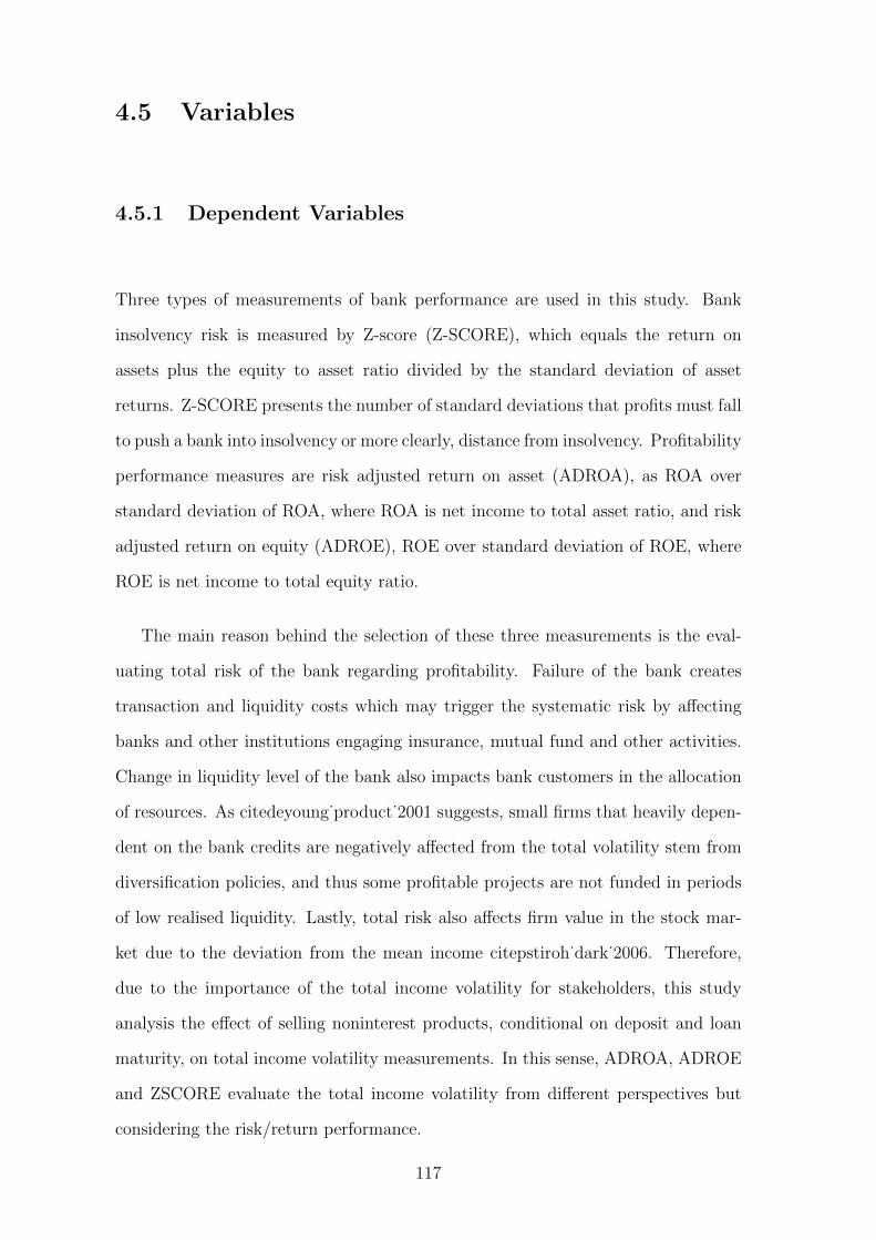
4.5 Variables

4.5.1 Dependent Variables

Three types of measurements of bank performance are used in this study. Bank

insolvency risk is measured by Z-score (Z-SCORE), which equals the return on

assets plus the equity to asset ratio divided by the standard deviation of asset

returns. Z-SCORE presents the number of standard deviations that profits must fall

to push a bank into insolvency or more clearly, distance from insolvency. Profitability

performance measures are risk adjusted return on asset (ADROA), as ROA over

standard deviation of ROA, where ROA is net income to total asset ratio, and risk

adjusted return on equity (ADROE), ROE over standard deviation of ROE, where

ROE is net income to total equity ratio.

The main reason behind the selection of these three measurements is the eval-

uating total risk of the bank regarding profitability. Failure of the bank creates

transaction and liquidity costs which may trigger the systematic risk by affecting

banks and other institutions engaging insurance, mutual fund and other activities.

Change in liquidity level of the bank also impacts bank customers in the allocation

of resources. As citedeyoung˙product˙2001 suggests, small firms that heavily depen-

dent on the bank credits are negatively affected from the total volatility stem from

diversification policies, and thus some profitable projects are not funded in periods

of low realised liquidity. Lastly, total risk also affects firm value in the stock mar-

ket due to the deviation from the mean income citepstiroh˙dark˙2006. Therefore,

due to the importance of the total income volatility for stakeholders, this study

analysis the effect of selling noninterest products, conditional on deposit and loan

maturity, on total income volatility measurements. In this sense, ADROA, ADROE

and ZSCORE evaluate the total income volatility from different perspectives but

considering the risk/return performance.

117

4.5.2 Explanatory Variables

Deposit Diversification (HHIDEP) : Maturity diversification for deposit is

measured by Herfindahl Hirschman Index. The formula is given by

HHIDEP = (STD

TD)2 + (

LTD

TD)2 (4.5)

where STD denotes short term deposits by banks and customers with maturity

between 0 and 1 year, LTD denotes long term deposits by banks and customers

with maturity of more than 1 year. TD is the annual basis total deposits of banks

and customers.

Long Term Deposits (LONGDEP) : measured by long term customer and

bank deposits divided by total deposit. Long term deposit is the customer deposit

with maturity of more than 1 year and total deposit is the sum of short and long

term deposits. It shows the effect of shifting maturity of deposits from short term

to long term.

Lag of Long Term Deposit Ratio (LAGDEP) : the lag value of LONGDEP.

Rather than direct impact, its interactions with non-interest income activities are

expected to be significant in explaining bank performance.

Capitalization (CAPITAL) : total equity to total asset ratio is introduced to

see the effect of equity. It is priori expected to result in a positive relationship

between equity and bank risk.

HHICOM : the effect of market competition on risk, measured by HHI index.

HHICOM is the sum of the squares of the bank size shares measured by total assets

to total banking sector assets.

118

INTERESTASSET : measured by net interest income to total assets ratio. In-

terest income and non-interest income are not used to calculate HHI index. Because

bank interest and non-interest income include many values lower than 0 as com-

ponents of total income, interest income over total income and non-interest income

over total income ratios take values lower than 0 or higher than 1. Thus, measuring

the effect with these values is a barrier against in true determination of causality.

Moreover, this study draws attention to subcategories of total income and their in-

teraction with maturity variables. As such, net interest income over total asset is

preferred rather than HHI index.

Fees and Commissions (FEES) : net fees and commissions to total net non-

interest income ratio is introduced to measure the effect of fees and commissions as

a component of non-interest income.

Trade Income (TRADE) : the effect of trade income on bank risk is measured

by trade income to total asset ratio.

Staff Expense (STAFFEXPENSE) : shows the effect of staff expense on per-

formance. Staff expense is measured by staff expense to operating expense ratio.

Asset Size (LNASSET) : measures logarithm of total asset. This variable is

included to control for the effect of bank size.

Loan Diversification (HHILOAN) : maturity diversification for loan is also

measured by the Herfindahl Hirschman Index. Its formula is given by

HHIDEP = (STL

TL)2 + (

LTL

TL)2 (4.6)

where STL denotes short term loans and advances to banks and customers with

maturity between 0 and 1 year, LTL denotes long term loans and advances to banks

119

and customers with maturity of more than 1 year. TL is the annual basis total loans

given by banks.

Long Term Loans (LONGLOAN) : measured by long term loans and advances

to banks and customers divided by total loans. Long term loans are the loans and

advances to banks and customers with maturity of more than 1 year. Total loan is

the sum of short term and long term loans. It measures the effect of shifting loan

maturity from short term to long term on bank performance.

Lag of Long Term Loan Ratio (LAGLOAN) : the effect of the lag value of

long term loans. It is introduced especially for its indirect effect, conditional on fee

and trade incomes.

Second Lag of Long Term Loan Ratio (LAG2LOAN) : employed to see the

effect of the second lag value of long term loans. Likewise with LAGLOAN, it is

employed to see its indirect effect, conditional on fee and trade incomes.

INTERACTION TERMS

LONGDEPFEES : the effect of net fees and commissions, conditional on current

value of long term deposits. It is measured by LONGDEP x FEES.

LAGDEPFEES : the effect of lag value of long term deposits conditional on net

fees and commissions. It is measured by LAGDEP x FEES.

LONGLOANFEES : the effect of current value of long term loans conditional

on net fees and commissions, measured by LONGLOAN x FEES.

LAGLOANFEES : the effect of lag value of long term loans conditional on net

fees and commissions income. It is measured by LAGLOAN x FEES.

120

LAG2LOANFEES : interaction of second lag of the long term loans and current

value of fee income: LAG2LOAN x FEES.

LONGDEPTRADE : the effect of current value of long term deposits, condi-

tional on trade income. It is measured by LONGDEP x TRADE. This variable is

introduced to find an evidence for the effect of cross-selling policy of banks. Same

period cross-selling and bundling are subject to same type of income shocks and

may negatively impact bank performance.

LAGDEPTRADE : the effect of lag value of long term deposits conditional on

trade income, measured by LAGDEP x TRADE.

LONGLOANTRADE : the effect of current value of long term loans conditional

on trade income. It is measured by LONGLOAN x TRADE. Potential same sign

with LONGDEPTRADE provides evidence for increasing risk stemmed from income

shock for both traditional and non-traditional income sides.

LAGLOANTRADE : the effect of lag value of long term loans conditional on

trade income. It is measured by LAGLOAN x TRADE. Since long term customers

stay at the same bank for more than one year, banks may improve their communi-

cation by time and hence increases the likelihood of selling non-traditional products

in the following years of where loan transaction started.

LAG2LOANTRADE : this variable is the construction of the second lag value of

the long term loans and current value of trade income to see the effect of cross-selling

of trade product in the second year of long term loan: LAG2LOAN x TRADE

For the years 2007, 2008 and 2009, time dummies are created due to the financial

crisis in the UK.

121

4.6 Methodology for Empirical Study

Coefficients are estimated by two-step system GMM methodology that combines

the differenced equations and level equations. Generally, banking data, particularly

profit and risk data, includes dynamic association between dependent variable and

its lag value. The dynamic approach is captured by the GMM estimator (Baltagi,

2008)

Another reason is the potential endogeneity problem that can be solved by Sys-

tem GMM. Endogeneity is expected between dependent variables and some explana-

tory variables, such as diversification variables.

Some factors that may explain the bank performance are difficult to measure,

such as managerial capability. To avoid problems stem from unobserved heterogene-

ity, and thus biased results, the system GMM is preferred.

In this study, two specification tests are reported below to the tables. The first

test is the auto-correlation test for disturbance term: First order autocorrelation

and second order autocorrelation. Estimates are consistent if first order autocorre-

lation is available in the differenced residuals, but unavailable in the second order

autocorrelation. The second test reported in this study is the Hansen test for over-

identifying restrictions that examines the validity of instruments. Considering the

small sample used in the study, the two-step standard errors are computed in ac-

cordance to the Windmeijer (2005) finite-sample correction.

4.7 Results

Table 4.1 presents the descriptive statistics for variables. The numbers indicate

the ups and downs for three measurements covering the period 2005 and 2012. Z-

SCORE reaches its lowest mean value in 2008, but deviation is highest at 2007.

Then, mean value steadily increases up to last observation year 2012. This year

is the peak point for sample period. However, ups and downs are clearer for the

profitability measurements; ADROA and ADROE. ADROA reaches its minimum

122

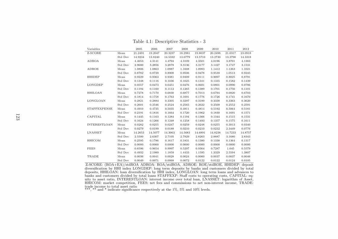
Table 4.1: Descriptive Statistics - 3

Variables 2005 2006 2007 2008 2009 2010 2011 2012

Z-SCORE Mean 21.2491 19.2047 20.3237 18.2981 19.8037 20.2498 21.0317 23.0918

Std Dev 14.9234 13.8240 14.5592 13.6779 13.5710 13.2730 13.3790 14.3318

ADROA Mean 4.4653 4.3141 4.4794 4.3109 4.3501 4.0196 3.8701 4.1383

Std Dev 2.9680 3.2856 3.2878 3.3136 3.3177 3.1427 3.1747 3.1531

ADROE Mean 1.0806 1.0863 1.0987 1.1608 1.0983 1.1412 1.1263 1.1021

Std Dev 0.8782 0.8729 0.8908 0.9506 0.9478 0.9539 1.0513 0.9245

HHIDEP Mean 0.9229 0.9363 0.9381 0.9409 0.9111 0.9097 0.8825 0.8791

Std Dev 0.1348 0.1116 0.1036 0.1025 0.1341 0.1335 0.1582 0.1439

LONGDEP Mean 0.0557 0.0473 0.0451 0.0476 0.0681 0.0801 0.0990 0.0786

Std Dev 0.1194 0.1160 0.1112 0.1265 0.1389 0.1701 0.1756 0.1101

HHILOAN Mean 0.7278 0.7170 0.6830 0.6877 0.7013 0.6794 0.6820 0.6703

Std Dev 0.1814 0.1758 0.1763 0.1691 0.1776 0.1726 0.1741 0.1670

LONGLOAN Mean 0.2821 0.2884 0.3305 0.3297 0.3189 0.3338 0.3363 0.3620

Std Dev 0.2601 0.2546 0.2524 0.2565 0.2622 0.2509 0.2552 0.2591

STAFFEXPENSE Mean 0.4910 0.4735 0.5035 0.4811 0.4814 0.5192 0.5064 0.5181

Std Dev 0.2191 0.1816 0.1664 0.1720 0.1962 0.1830 0.1691 0.1571

CAPITAL Mean 0.1445 0.1163 0.1284 0.1194 0.1366 0.1344 0.1515 0.1531

Std Dev 0.1624 0.1266 0.1248 0.1258 0.1493 0.1357 0.1575 0.1611

INTERESTLOAN Mean 0.0282 0.0255 0.0247 0.0259 0.0248 0.0255 0.3013 0.0340

Std Dev 0.0279 0.0199 0.0188 0.0210 0.0210 0.0232 2.3449 0.0776

LNASSET Mean 14.2653 14.5077 14.3063 14.5683 14.6891 14.8238 14.7233 14.8757

Std Dev 2.5500 2.6307 2.7105 2.7929 2.8263 2.8887 3.1680 2.8343

HHICOM Mean 0.2595 0.1786 0.1617 0.1831 0.1380 0.1338 0.1364 0.1317

Std Dev 0.0000 0.0000 0.0000 0.0000 0.0000 0.0000 0.0000 0.0000

FEES Mean 0.6596 0.9654 0.9997 0.5297 0.9364 0.7287 1.045 0.5579

Std Dev 0.4932 2.1989 1.1859 1.4433 1.1595 1.3329 2.5594 1.3807

TRADE Mean 0.0036 0.0041 0.0028 0.0024 0.0060 0.0037 0.0037 0.0046

Std Dev 0.0049 0.0071 0.0068 0.0072 0.0122 0.0122 0.0124 0.0105

Z-SCORE: (ROA+EA)/stdROA ADROA: ROA/stdROA, ADROE: ROE/stdROE, HHIDEP: depositdiversification by HHI index LONGDEP: long term deposits by banks and customers divided by totaldeposits, HHILOAN: loan diversification by HHI index, LONGLOAN: long term loans and advances tobanks and customers divided by total loans STAFFEXP: Staff costs to operating costs, CAPITAL: eq-uity to asset ratio, INTERESTLOAN: interest income over total loan, LNASSET: logarithm of Asset,HHICOM: market competition, FEES: net fees and commissions to net non-interest income, TRADE:trade income to total asset ratio***, ** and * indicate significance respectively at the 1%, 5% and 10% levels.

123

value at 2010, while ADROE reaches at 2005.

For deposit diversification, HHIDEP, it is seen that diversification decreases until

2008. Then diversification is in upward trend by falling from 0.94 to 0.87. Deposit

diversification decreases during 2005 - 2008 period and then increases steadily for

the period 2009 - 2012. On the contrary, loan diversification is an increasing trend

for 2005 - 2008 period and followed by ups and downs. The change in mean values of

deposit and loan diversification are not correlated. The correlation between deposit

and loan diversification is 23%, which is not too high to match supply and demand

sides. Another interesting result seen from deposit and loan diversification is that

loan diversification is greater than deposit diversification. Moreover, the standard

deviation of the loan diversification is relatively higher, too.

The differences in diversification are seen more clearly in the variables LONGDEP

and LONGLOAN ratios. The share of the long-term deposits is around 5%, but av-

erage for long-term loan share is around 30%. There is no trend for the long-term

deposits but Table 4.1 depicts an upward trend for long-term loans from 2005 to

2012. It steadily reaches 36% from 28% between the years 2005 and 2012. This

trend shows that share of the long-term loans increased during this period.

The competition level provides interesting trends. The HHICOM values decrease

during this period by falling from 0.26 to 0.13. The decrease implies the increase

in competition during this period, especially after 2008 financial crisis. Table 4.1

states that as the competition increase, the capital of the banks increases too.

Before the supply and demand side results, it is correct to note that the three

measurements are not perfectly correlated. Therefore, different results are expected

for some explanatory variables.

4.7.1 Supply Side Results

Table 4.2 presents the six estimations for the supply side bank performance using

three performance measures. Table 4.2 shows the effects of interaction of deposit

maturities with non-interest income components.

124

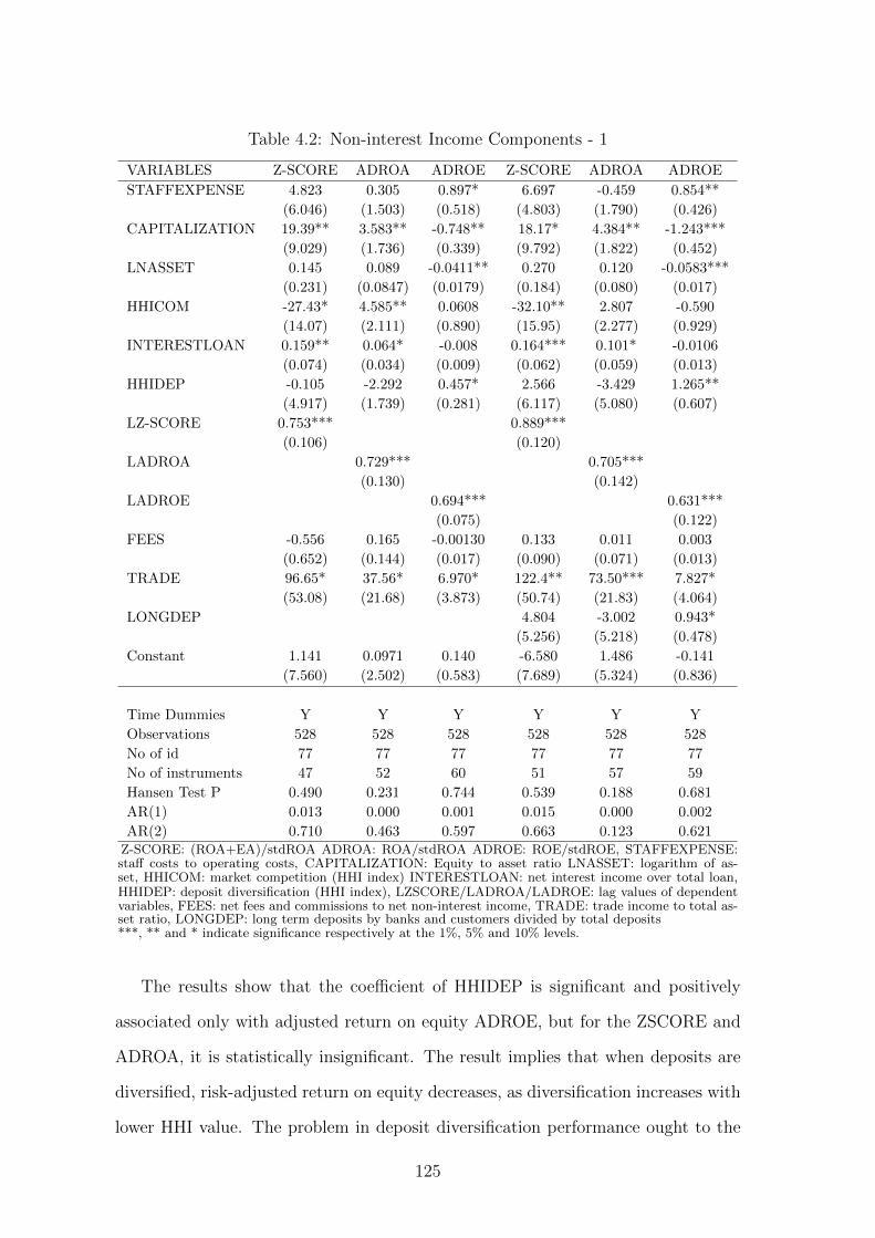
Table 4.2: Non-interest Income Components - 1

VARIABLES Z-SCORE ADROA ADROE Z-SCORE ADROA ADROE

STAFFEXPENSE 4.823 0.305 0.897* 6.697 -0.459 0.854**

(6.046) (1.503) (0.518) (4.803) (1.790) (0.426)

CAPITALIZATION 19.39** 3.583** -0.748** 18.17* 4.384** -1.243***

(9.029) (1.736) (0.339) (9.792) (1.822) (0.452)

LNASSET 0.145 0.089 -0.0411** 0.270 0.120 -0.0583***

(0.231) (0.0847) (0.0179) (0.184) (0.080) (0.017)

HHICOM -27.43* 4.585** 0.0608 -32.10** 2.807 -0.590

(14.07) (2.111) (0.890) (15.95) (2.277) (0.929)

INTERESTLOAN 0.159** 0.064* -0.008 0.164*** 0.101* -0.0106

(0.074) (0.034) (0.009) (0.062) (0.059) (0.013)

HHIDEP -0.105 -2.292 0.457* 2.566 -3.429 1.265**

(4.917) (1.739) (0.281) (6.117) (5.080) (0.607)

LZ-SCORE 0.753*** 0.889***

(0.106) (0.120)

LADROA 0.729*** 0.705***

(0.130) (0.142)

LADROE 0.694*** 0.631***

(0.075) (0.122)

FEES -0.556 0.165 -0.00130 0.133 0.011 0.003

(0.652) (0.144) (0.017) (0.090) (0.071) (0.013)

TRADE 96.65* 37.56* 6.970* 122.4** 73.50*** 7.827*

(53.08) (21.68) (3.873) (50.74) (21.83) (4.064)

LONGDEP 4.804 -3.002 0.943*

(5.256) (5.218) (0.478)

Constant 1.141 0.0971 0.140 -6.580 1.486 -0.141

(7.560) (2.502) (0.583) (7.689) (5.324) (0.836)

Time Dummies Y Y Y Y Y Y

Observations 528 528 528 528 528 528

No of id 77 77 77 77 77 77

No of instruments 47 52 60 51 57 59

Hansen Test P 0.490 0.231 0.744 0.539 0.188 0.681

AR(1) 0.013 0.000 0.001 0.015 0.000 0.002

AR(2) 0.710 0.463 0.597 0.663 0.123 0.621Z-SCORE: (ROA+EA)/stdROA ADROA: ROA/stdROA ADROE: ROE/stdROE, STAFFEXPENSE:staff costs to operating costs, CAPITALIZATION: Equity to asset ratio LNASSET: logarithm of as-set, HHICOM: market competition (HHI index) INTERESTLOAN: net interest income over total loan,HHIDEP: deposit diversification (HHI index), LZSCORE/LADROA/LADROE: lag values of dependentvariables, FEES: net fees and commissions to net non-interest income, TRADE: trade income to total as-set ratio, LONGDEP: long term deposits by banks and customers divided by total deposits***, ** and * indicate significance respectively at the 1%, 5% and 10% levels.

The results show that the coefficient of HHIDEP is significant and positively

associated only with adjusted return on equity ADROE, but for the ZSCORE and

ADROA, it is statistically insignificant. The result implies that when deposits are

diversified, risk-adjusted return on equity decreases, as diversification increases with

lower HHI value. The problem in deposit diversification performance ought to the

125

lack of power of banks to shift the directions of maturities. Depositors may be inelas-

tic against to change maturity of their deposits. Banks may be politically insufficient

to diversify their deposits corresponding to their loan plan, and therefore, deposits

are relatively out of control. To elaborate further, the deposits are short-term in

most cases which implies that deposit customers are also short-term customers.

Second, deposits are just one instrument to supply sources for loans. Banks

can provide other sources, and henceforth diversification of deposits may not signifi-

cantly contribute to the performance if other sources are not costly enough. Having

different sources instead of deposits may allow banks to draw less attention to the

deposit diversification. As clarified by Altunbas et al. (2011), deregulation and in-

novations help the bank to alleviate the need for financial markets for their funding.

The advantage of the financial markets, such as interbank markets, certificate of

deposits and short-term bonds, is that banks can borrow more easily from these

markets. Moreover, the deposits are relatively less than the potential in financial

market so that they can borrow with large amounts (Altunbas et al., 2011). Easily

borrowing from markets by a large amount is used to fund, probably, long term

loans. Shares of the long-term deposits and loans are far away from matching. The

sum of total long-term deposits is around half of the long-term loans. Calomiris and

Kahn (1991) point out that financial market investors are relatively more sophisti-

cated than depositors who create a market discipline. Demirguc-Kunt and Huizinga

(2010) find that use of non-deposit funding is more common in developed countries.

For these reasons, banks possibly give more consideration to the alternative sources

and thereby deposit diversification is insignificant in explaining market risk.

Similar to HHIDEP, STAFFEXPENSE is positively associated with the risk-

adjusted return on equity. This variable is insignificant for both ZSCORE and

ADROA. The effect of the CAPITALIZATION variable is interesting: it affects the

different dependent variable with the opposite sign. CAPITALIZATION increases

the bank performance for ZSCORE and ADROA. However, it is inversely related

with ADROE. These opposite results confirm the findings by

126

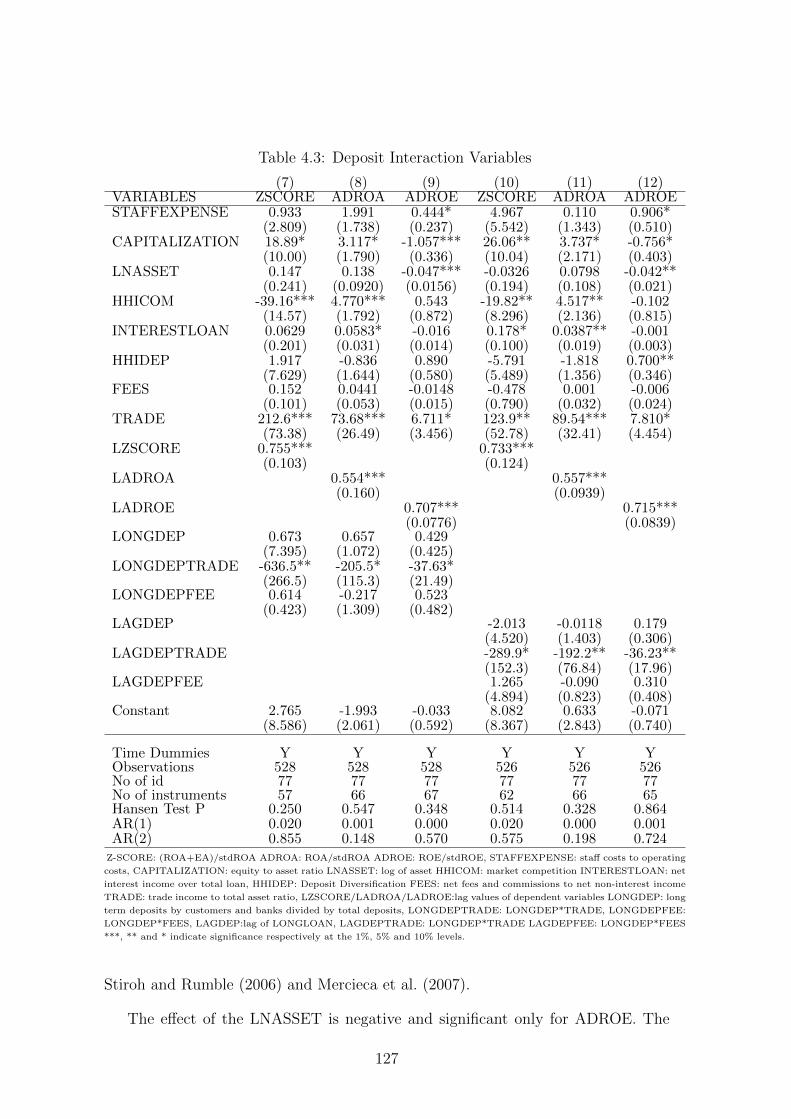
Table 4.3: Deposit Interaction Variables

(7) (8) (9) (10) (11) (12)VARIABLES ZSCORE ADROA ADROE ZSCORE ADROA ADROESTAFFEXPENSE 0.933 1.991 0.444* 4.967 0.110 0.906*

(2.809) (1.738) (0.237) (5.542) (1.343) (0.510)CAPITALIZATION 18.89* 3.117* -1.057*** 26.06** 3.737* -0.756*

(10.00) (1.790) (0.336) (10.04) (2.171) (0.403)LNASSET 0.147 0.138 -0.047*** -0.0326 0.0798 -0.042**

(0.241) (0.0920) (0.0156) (0.194) (0.108) (0.021)HHICOM -39.16*** 4.770*** 0.543 -19.82** 4.517** -0.102

(14.57) (1.792) (0.872) (8.296) (2.136) (0.815)INTERESTLOAN 0.0629 0.0583* -0.016 0.178* 0.0387** -0.001

(0.201) (0.031) (0.014) (0.100) (0.019) (0.003)HHIDEP 1.917 -0.836 0.890 -5.791 -1.818 0.700**

(7.629) (1.644) (0.580) (5.489) (1.356) (0.346)FEES 0.152 0.0441 -0.0148 -0.478 0.001 -0.006

(0.101) (0.053) (0.015) (0.790) (0.032) (0.024)TRADE 212.6*** 73.68*** 6.711* 123.9** 89.54*** 7.810*

(73.38) (26.49) (3.456) (52.78) (32.41) (4.454)LZSCORE 0.755*** 0.733***

(0.103) (0.124)LADROA 0.554*** 0.557***

(0.160) (0.0939)LADROE 0.707*** 0.715***

(0.0776) (0.0839)LONGDEP 0.673 0.657 0.429

(7.395) (1.072) (0.425)LONGDEPTRADE -636.5** -205.5* -37.63*

(266.5) (115.3) (21.49)LONGDEPFEE 0.614 -0.217 0.523

(0.423) (1.309) (0.482)LAGDEP -2.013 -0.0118 0.179

(4.520) (1.403) (0.306)LAGDEPTRADE -289.9* -192.2** -36.23**

(152.3) (76.84) (17.96)LAGDEPFEE 1.265 -0.090 0.310

(4.894) (0.823) (0.408)Constant 2.765 -1.993 -0.033 8.082 0.633 -0.071

(8.586) (2.061) (0.592) (8.367) (2.843) (0.740)

Time Dummies Y Y Y Y Y YObservations 528 528 528 526 526 526No of id 77 77 77 77 77 77No of instruments 57 66 67 62 66 65Hansen Test P 0.250 0.547 0.348 0.514 0.328 0.864AR(1) 0.020 0.001 0.000 0.020 0.000 0.001AR(2) 0.855 0.148 0.570 0.575 0.198 0.724

Z-SCORE: (ROA+EA)/stdROA ADROA: ROA/stdROA ADROE: ROE/stdROE, STAFFEXPENSE: staff costs to operating

costs, CAPITALIZATION: equity to asset ratio LNASSET: log of asset HHICOM: market competition INTERESTLOAN: net

interest income over total loan, HHIDEP: Deposit Diversification FEES: net fees and commissions to net non-interest income

TRADE: trade income to total asset ratio, LZSCORE/LADROA/LADROE:lag values of dependent variables LONGDEP: long

term deposits by customers and banks divided by total deposits, LONGDEPTRADE: LONGDEP*TRADE, LONGDEPFEE:

LONGDEP*FEES, LAGDEP:lag of LONGLOAN, LAGDEPTRADE: LONGDEP*TRADE LAGDEPFEE: LONGDEP*FEES

***, ** and * indicate significance respectively at the 1%, 5% and 10% levels.

Stiroh and Rumble (2006) and Mercieca et al. (2007).

The effect of the LNASSET is negative and significant only for ADROE. The

127

negative coefficient implies that deviation increases over bank size. For others, it is

statistically insignificant. Similar to LNASSET, HHICOM is statistically significant

for only one dependent variable; ZSCORE. When the competition increases, bank’s

income becomes more stable.

Table 4.2 also reports lag values of the dependent variables. Results indicate that

they are statistically highly significant, and their signs are positive for all three types

of measurements. Hence, current adjusted bank performance is positively linked

with past realization of bank performance which implies a dynamic relationship.

Non-interest income includes different products that are characteristically differ-

ent than each other or from another view; non-interest products are priced differ-

ently and used for different policies. Testing non-interest products by disaggregating

them as fee and trade products allows us to understand causalities of each line of

income separately. Table 4.2 reports the effects of non-interest income components

and share of the long-term deposits. Now, non-interest income is decomposed as

FEES and TRADE. Results state that higher dependence on FEES is statistically

insignificant to explain risk-adjusted bank performance. However, different than the

literature, greater reliance on TRADE is positive and significant for all three types of

measurements of bank performance. This result implies that despite the results that

finding a negative association between TRADE and bank performance in the liter-

ature, TRADE no longer has an adverse effect on risk-adjusted bank performance.

In the literature, it is seen that most of the studies present the 1990’s whilst this

study grasps the more recent period. Banks may adjust their trade product strate-

gies through the increasing trend in sales of trade product. Also, transformation of

its structure, new non-interest products and advances in technology are the other

factors that may contribute to less deviation in trade income. In addition, banks

gain knowledge about trading, especially small banks were not familiar with the

trading activities in 1990’s. Banks possibly now more experienced than the 1990’s.

Alternatively, the period examined in this study includes the crisis and post-crisis

periods. Compared to interest and fee income channels, trade income may be less

128

dependent on overall business conditions.

Another income component, INTERESTLOAN, is statistically significant, and

its effect is positive to the performance. As DeYoung and Roland (2001) suggest,

shifting banks for lending activity is costly for the customer. Information, search

and other switching costs are the barriers changing banks for lending activity hence,

making interest income more stable. The only problem with income components

is the fees and commissions, during the period 2005 and 2012. The fee income

is significantly affected by loan market, as well as the fee market, and is open to

different pricing strategies as a complement product. Using fee products for multiple

pricing may prevent diversification benefits from the shifting loan side to the fee

income side.

Table 4.3 presents the interaction variables which show the indirect effect of de-

posit maturity. Similar to the FEES variable, LONGDEPFEES and LAGDEPFEES

are also insignificant in explaining bank performance. Since fees and commissions

policy consists of many pricing strategies, its effects may not reflect these poli-

cies. The lack of the data for fees and commissions charged from different pricing

strategies is a barrier to differentiating fee policies. However, for all three measure-

ments, LONGDEPTRADE is statistically significant. As models 10 to 12 depict,

LAGDEPTRADE is also statistically significant for all three measures. Improve-

ments in communication between the bank and long-term depositors increase the

probability of cross-selling to these long-term customers. In other words, if banks

assume that long-term depositors are more creditworthy, then, they may have an

incentive to sell non-interest products. However, at this point, any income shock

to the depositor may affect both deposits and non-interest income side by lowering

the deposits and creating a payment problem in non-interest income side. Hence,

cross-selling to the core depositor negatively affects bank performance.

129

4.7.2 Demand Side Results

Table 4.4 presents the six estimations regarding the implication of the demand side

on bank performance. According to the results in Table 4.4, loan diversification is

positively associated with Z-SCORE and ADROA. Banks have more instruments

and choices to diversify their loans by adjusting the interest rates for short- and

long-terms loans. Compared to depositors, banks possibly find short- and long-term

loan customers for intermediation activity easier. Therefore, they can benefit from

loan diversification utilising interest rate policies.

Table 4.5 presents the interaction of long-term loan share with fee income (LON-

GLOANFEE) and trade income (LONGLOANTRADE). The results indicate that

the effect of fees income conditional on the long-term loans is statistically significant,

but its effect is negative. The trade income positively affects bank performance, but

the interaction of trade income with long term loan negatively impacts bank per-

formance. This result implies that the positive effect of the trade income becomes

negative, conditional on long-term loan. The main reason behind these opposite

signs is likely related to banks’ selling trade products to the long-term customer

using bundling and cross-selling policies. Since the long-term customer and bank

relationship includes improvements in communications, such as arm length relation-

ship, similar to long-term depositors, it is expected to provide an incentive for banks

to engage in non-interest product sale to the long-term loan customers. The power

and ability of persuasion of banks increases over time and banks would like to use

this condition to its advantage by cross-selling. However, this is an increase of the

transaction volume or a similar case to increase in loan size and as such, increase

in the risk of the bank. From the portfolio perspective, it increases the correlation

coefficient between interest and non-interest income, which implies an increase in

risk for the bank.

Banks may struggle to sell diversified products not only in the current period

but also following years of the relationship with long-term loan customers (i.e. more

than one year). Thus, they may be persuaded to perform a cross-selling transaction

130

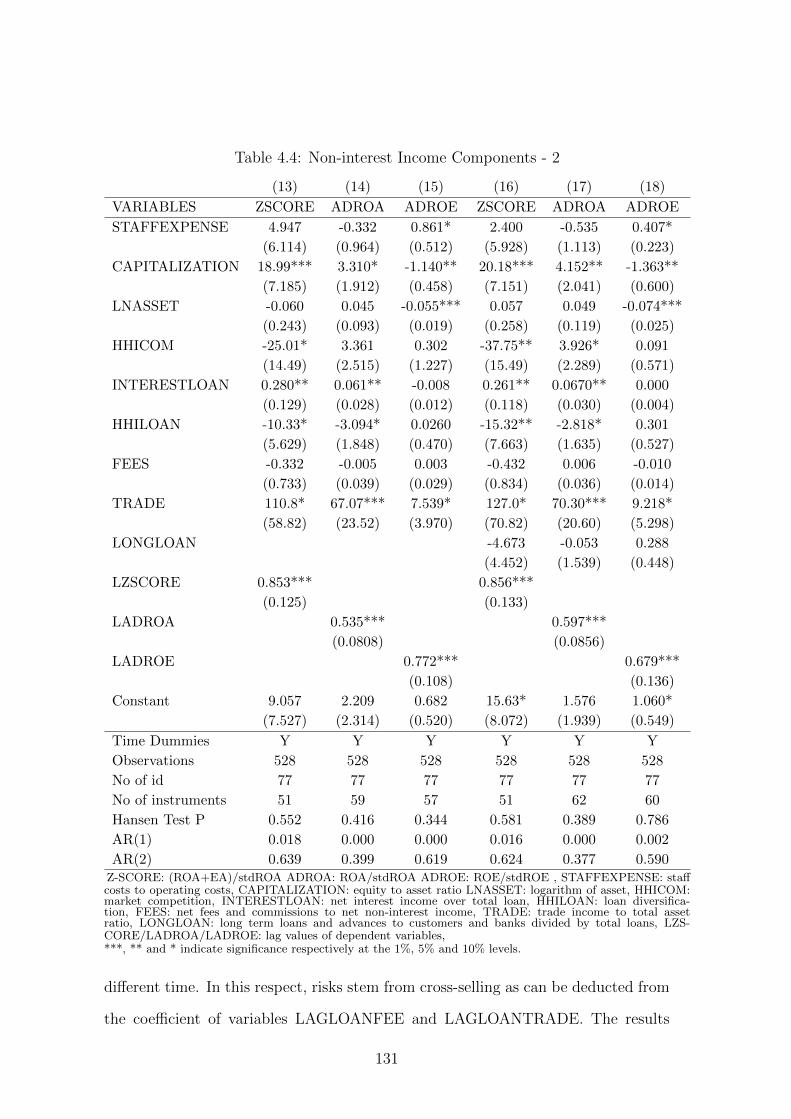
Table 4.4: Non-interest Income Components - 2

(13) (14) (15) (16) (17) (18)

VARIABLES ZSCORE ADROA ADROE ZSCORE ADROA ADROE

STAFFEXPENSE 4.947 -0.332 0.861* 2.400 -0.535 0.407*

(6.114) (0.964) (0.512) (5.928) (1.113) (0.223)

CAPITALIZATION 18.99*** 3.310* -1.140** 20.18*** 4.152** -1.363**

(7.185) (1.912) (0.458) (7.151) (2.041) (0.600)

LNASSET -0.060 0.045 -0.055*** 0.057 0.049 -0.074***

(0.243) (0.093) (0.019) (0.258) (0.119) (0.025)

HHICOM -25.01* 3.361 0.302 -37.75** 3.926* 0.091

(14.49) (2.515) (1.227) (15.49) (2.289) (0.571)

INTERESTLOAN 0.280** 0.061** -0.008 0.261** 0.0670** 0.000

(0.129) (0.028) (0.012) (0.118) (0.030) (0.004)

HHILOAN -10.33* -3.094* 0.0260 -15.32** -2.818* 0.301

(5.629) (1.848) (0.470) (7.663) (1.635) (0.527)

FEES -0.332 -0.005 0.003 -0.432 0.006 -0.010

(0.733) (0.039) (0.029) (0.834) (0.036) (0.014)

TRADE 110.8* 67.07*** 7.539* 127.0* 70.30*** 9.218*

(58.82) (23.52) (3.970) (70.82) (20.60) (5.298)

LONGLOAN -4.673 -0.053 0.288

(4.452) (1.539) (0.448)

LZSCORE 0.853*** 0.856***

(0.125) (0.133)

LADROA 0.535*** 0.597***

(0.0808) (0.0856)

LADROE 0.772*** 0.679***

(0.108) (0.136)

Constant 9.057 2.209 0.682 15.63* 1.576 1.060*

(7.527) (2.314) (0.520) (8.072) (1.939) (0.549)

Time Dummies Y Y Y Y Y Y

Observations 528 528 528 528 528 528

No of id 77 77 77 77 77 77

No of instruments 51 59 57 51 62 60

Hansen Test P 0.552 0.416 0.344 0.581 0.389 0.786

AR(1) 0.018 0.000 0.000 0.016 0.000 0.002

AR(2) 0.639 0.399 0.619 0.624 0.377 0.590Z-SCORE: (ROA+EA)/stdROA ADROA: ROA/stdROA ADROE: ROE/stdROE , STAFFEXPENSE: staffcosts to operating costs, CAPITALIZATION: equity to asset ratio LNASSET: logarithm of asset, HHICOM:market competition, INTERESTLOAN: net interest income over total loan, HHILOAN: loan diversifica-tion, FEES: net fees and commissions to net non-interest income, TRADE: trade income to total assetratio, LONGLOAN: long term loans and advances to customers and banks divided by total loans, LZS-CORE/LADROA/LADROE: lag values of dependent variables,***, ** and * indicate significance respectively at the 1%, 5% and 10% levels.

different time. In this respect, risks stem from cross-selling as can be deducted from

the coefficient of variables LAGLOANFEE and LAGLOANTRADE. The results

131

state that the LAGLOANFEE is statistically insignificant revealing the adverse

effect of the fees income conditional on long-term loan on bank performance. The

logic behind this relationship may be associated with the fees and commissions

charged during the loan application process. Banks are inclined to charge fees and

commissions to compensate losses from lower loan prices, and generally, customers

are unable to escape such a set-up as fees are an inseparable part of the lending

activity. Secondly, the complement fee products may be sold in the application

period by bundling strategy. In this structure, any income shocks to customers

affect both parts of the income statement and negatively affects bank performance.

Most of the long-term loans require fee transactions associated with the aim of

using that loan. Furthermore, they may be higher in volume. For example, long-

term housing credits require a broad range of fee activities during the application

period, the size of both fees and loans are very high. The insignificance in later

periods as the result shows imply the flexibility effect of customers.

Similar to LONGLOANTRADE, LAGLOANTRADE is also statistically signifi-

cant, and its effect is negative for all three measures. Moreover, LAG2LOANTRADE

is also statistically significant for the three measures. As such, long-term rela-

tionships with loan customer conditional on trade income contributes to low bank

performance. The significance of LONGLOANTRADE, LAGLOANTRADE and

LAG2LOANTRADE provides substantial evidence for the probability of bundling

(for LONGLOANTRADE) and other cross-selling policies, conditional on loan ma-

turity.

These empirical results also imply that the effect of efficient monitoring is not a

dominant factor in increasing bank performance in cross-selling. Sometimes, banks

fail to monitor their customers or score them improperly. The reason behind the

issue may be related to the ability and motivation of the sales forces (Jarrar and

Neely, 2002). Banks use technology and some mathematical modelling and provide

information. This information is analysed by employees and requires appropriate

132

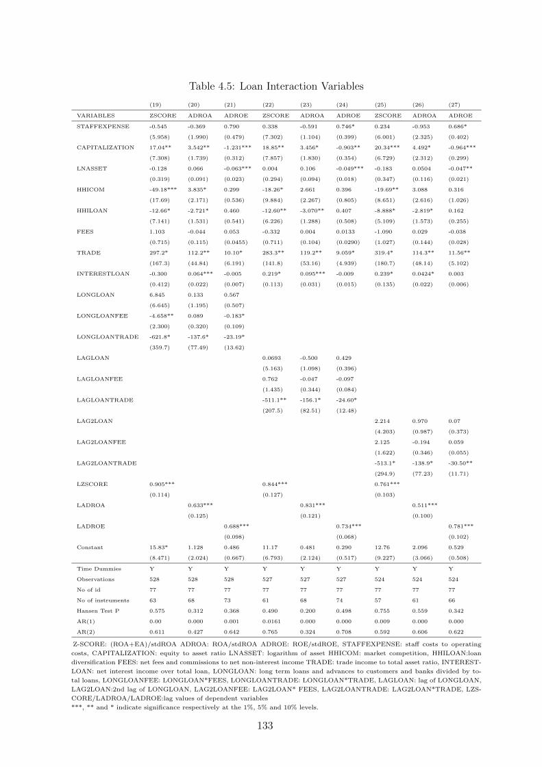
Table 4.5: Loan Interaction Variables

(19) (20) (21) (22) (23) (24) (25) (26) (27)

VARIABLES ZSCORE ADROA ADROE ZSCORE ADROA ADROE ZSCORE ADROA ADROE

STAFFEXPENSE -0.545 -0.369 0.790 0.338 -0.591 0.746* 0.234 -0.953 0.686*

(5.958) (1.990) (0.479) (7.302) (1.104) (0.399) (6.001) (2.325) (0.402)

CAPITALIZATION 17.04** 3.542** -1.231*** 18.85** 3.456* -0.903** 20.34*** 4.492* -0.964***

(7.308) (1.739) (0.312) (7.857) (1.830) (0.354) (6.729) (2.312) (0.299)

LNASSET -0.128 0.066 -0.063*** 0.004 0.106 -0.049*** -0.183 0.0504 -0.047**

(0.319) (0.091) (0.023) (0.294) (0.094) (0.018) (0.347) (0.116) (0.021)

HHICOM -49.18*** 3.835* 0.299 -18.26* 2.661 0.396 -19.69** 3.088 0.316

(17.69) (2.171) (0.536) (9.884) (2.267) (0.805) (8.651) (2.616) (1.026)

HHILOAN -12.66* -2.721* 0.460 -12.60** -3.070** 0.407 -8.888* -2.819* 0.162

(7.141) (1.531) (0.541) (6.226) (1.288) (0.508) (5.109) (1.573) (0.255)

FEES 1.103 -0.044 0.053 -0.332 0.004 0.0133 -1.090 0.029 -0.038

(0.715) (0.115) (0.0455) (0.711) (0.104) (0.0290) (1.027) (0.144) (0.028)

TRADE 297.2* 112.2** 10.10* 283.3** 119.2** 9.059* 319.4* 114.3** 11.56**

(167.3) (44.84) (6.191) (141.8) (53.16) (4.939) (180.7) (48.14) (5.102)

INTERESTLOAN -0.300 0.064*** -0.005 0.219* 0.095*** -0.009 0.239* 0.0424* 0.003

(0.412) (0.022) (0.007) (0.113) (0.031) (0.015) (0.135) (0.022) (0.006)

LONGLOAN 6.845 0.133 0.567

(6.645) (1.195) (0.507)

LONGLOANFEE -4.658** 0.089 -0.183*

(2.300) (0.320) (0.109)

LONGLOANTRADE -621.8* -137.6* -23.19*

(359.7) (77.49) (13.62)

LAGLOAN 0.0693 -0.500 0.429

(5.163) (1.098) (0.396)

LAGLOANFEE 0.762 -0.047 -0.097

(1.435) (0.344) (0.084)

LAGLOANTRADE -511.1** -156.1* -24.60*

(207.5) (82.51) (12.48)

LAG2LOAN 2.214 0.970 0.07

(4.203) (0.987) (0.373)

LAG2LOANFEE 2.125 -0.194 0.059

(1.622) (0.346) (0.055)

LAG2LOANTRADE -513.1* -138.9* -30.50**

(294.9) (77.23) (11.71)

LZSCORE 0.905*** 0.844*** 0.761***

(0.114) (0.127) (0.103)

LADROA 0.633*** 0.831*** 0.511***

(0.125) (0.121) (0.100)

LADROE 0.688*** 0.734*** 0.781***

(0.098) (0.068) (0.102)

Constant 15.83* 1.128 0.486 11.17 0.481 0.290 12.76 2.096 0.529

(8.471) (2.024) (0.667) (6.793) (2.124) (0.517) (9.227) (3.066) (0.508)

Time Dummies Y Y Y Y Y Y Y Y Y

Observations 528 528 528 527 527 527 524 524 524

No of id 77 77 77 77 77 77 77 77 77

No of instruments 63 68 73 61 68 74 57 61 66

Hansen Test P 0.575 0.312 0.368 0.490 0.200 0.498 0.755 0.559 0.342

AR(1) 0.00 0.000 0.001 0.0161 0.000 0.000 0.009 0.000 0.000

AR(2) 0.611 0.427 0.642 0.765 0.324 0.708 0.592 0.606 0.622

Z-SCORE: (ROA+EA)/stdROA ADROA: ROA/stdROA ADROE: ROE/stdROE, STAFFEXPENSE: staff costs to operating

costs, CAPITALIZATION: equity to asset ratio LNASSET: logarithm of asset HHICOM: market competition, HHILOAN:loan

diversification FEES: net fees and commissions to net non-interest income TRADE: trade income to total asset ratio, INTEREST-

LOAN: net interest income over total loan, LONGLOAN: long term loans and advances to customers and banks divided by to-

tal loans, LONGLOANFEE: LONGLOAN*FEES, LONGLOANTRADE: LONGLOAN*TRADE, LAGLOAN: lag of LONGLOAN,

LAG2LOAN:2nd lag of LONGLOAN, LAG2LOANFEE: LAG2LOAN* FEES, LAG2LOANTRADE: LAG2LOAN*TRADE, LZS-

CORE/LADROA/LADROE:lag values of dependent variables

***, ** and * indicate significance respectively at the 1%, 5% and 10% levels.

133

staff training at the end. Alternatively, even though banks correctly choose the

customers which they offer cross-selling, unexpected shocks may remove the success

in their selection. As it is seen from results, private information obtained by the

bank through longer maturity of loan does not help the bank to reduce risk in

cross-selling activities.

The reasons why banks shift to the non-interest income activities can be ex-

plained by the approach of Stiroh and Rumble (2006). Firstly, the expected and

actual returns can be different than each other, due to the unexpected shocks. Ig-

noring unexpected shocks may be accompanied by higher covariance coefficient.

Compared to expected return, the actual return may become lower due to these

shocks such as shocks associated with macroeconomic conditions or some particu-

lar sectors. Secondly, the managerial perception of diversification benefit may be

higher than the actual gain. The lack of information about the covariance between

interest and non-interest income may lead banks to diversify their income aggres-

sively through cross-selling. Moreover, earnings of the management may depend on

higher profits but any losses may be independent of the managerial earnings. Higher

earning managers without any risk bearing creates an incentive to take more risk.

Thirdly, a bank’s aim may not necessarily be profit maximization, such as conserv-

ing firm-specific human capitals or corporate control problems. Another explanation

suggested by Denis et al. (1997) and Rajan et al. (2000) is the agency problem be-

tween managers and owners, and power struggles between different segments within

a bank may lead to lower performance by cross-selling.

4.8 Conclusion

The aim of this study is to analyse the risk implications on the UK banking sec-

tor which has shifted away from traditional activities towards non-interest income

activities. To achieve its objective, the study investigates the impact of shifting

banks maturity diversification policies between short - and long-term loans and de-

posits. One of the main advantages of this study is that the UK deposit and loan

134

maturities are compiled from bank annual reports, and it is a very new and unique

data that has been used to analyse short and long-term deposit and loan maturi-

ties. Therefore, it is the first study to investigate the direct and indirect effects

of both deposit and loan maturities on bank performance. The results show that

cross-selling policies create risk through shifting deposits and loans from short- to

long-term. The fees and commissions variable in its own is insignificant to explain

banks’ performance, but fees and commission income associated with long-term loan

negatively affects bank performance. This negative relationship is valid only for the

same period. However, the interaction of fees with deposit maturity is insignificant.

It is reasonable to think that risk is associated with some complementary fees and

commissions for loans as well as the inseperable ones charged in the application

period of the long-term loan. The structure of the long-term loans allows the bank

to charge more fees and commission from transactions.

The trade income positively impacts risk-adjusted bank performance for all three

risk measures. In contrast, all the interaction variables of long-term maturity includ-

ing trade income are negatively associated with bank performance. The negative

coefficient of the interaction effect strengths the presence of potential problems such

as bundling and other cross-selling policies for the bank. Cross selling and bundling

strategies to the core customer are exposed to shocks, and it negatively affects both

the interest and trade income sides of the banks.

The findings reveal that deposit diversification neither improves nor reduces the

bank Z-score and risk-adjusted return on asset, but reduces the risk-adjusted return

on equity. The result implies that banks do not benefit from deposit diversification.

However, loan diversification improves banks’ performance measured by Z-score and

risk-adjusted return on asset. Studying the maturities of deposits and loans sep-

arately allows us to address the side that creates a barrier against diversification

benefit. The result postulates that for the British banking system, this side is the

deposit side which requires more attention from policy makers.

The policy implications of this study are threefold. First the diversification of

135

deposits appears unsatisfactory for the UK banking sector and banks should pay

deposit diversification policies more attention. Second, the income diversification

may alleviate bank risk. However, the excessive cross-selling pattern, conditional on

maturity, creates more risk for the bank. This study shows that increasing maturity

and cross-selling associated with longer maturity reduces the bank performance.

Bank should limit their cross-selling strategies. Also, banks need to improve their

monitoring capacity for cross-selling. Third banks should adopt robust techniques

to determine a cross-selling customer more appropriately and rigorously. Their risk

seems to stem from cross-selling increases by the maturity, and therefore, banks

should consider the risk of cross-selling on the maturities of deposits and loans.

Greater use of bundling and cross-selling by banks, and addressing it to the

same customer has risk implications whether or not the sale is made over one or two

periods. Thus selling traditional and non-traditional products and services sold in

different periods should also be considered in risk diversification models.

Concerning the overall risk associated with income components, banks should be

motivated, primarily to augment the fees and commission revenue side. However,

the positive effect of both interest and trade income variables warns us that banks

in the UK should focus on the fee and commission revenue sides to be more stable.

Reducing income volatility by improving the income diversification also helps banks

to reduce capital requirements in order to buffer risk. Therefore, the cross-selling

policy is also crucial for banks with respect to capital requirements.

For the regulators, it is seen that bank risk increases with maturity conditional

on cross-selling. This cross-selling strategy of bank increases the risk possibly due

to the higher covariance. As the covariance increases, the risk exposure from loan

size increases. There are no significant differences between risk with higher loan size

without cross-selling and risk with loan size but cross-selling of non-interest products

if the customer faces with income shock. In both cases, banks may have exposure

to liquidity risk or even bankruptcy risk subject to the total debt size. They should

increase the level of concentration to cross-selling without ignoring the importance

136

of total debt size.

The nature of the data does not allow differentiating bundling from other cross-

selling strategies. Periodical differences of cross-selling affect the debt size of the

customer. Bundling is implemented when loan debt size of the customer is in the

maximum amount. However, cross-selling excluding bundling may arise following

periods of the loan transaction. Compared to bundling, this implies the lower debt

size. Any income shock to the second case is expected to be less risky for banks.

Further researches should be devoted to the analysis of differences in these strategies

beyond the risk stem from general cross-selling. Also, further researches should

focus on the comparisons between relationship banking and transactional banking.

Relationship banking is subject to borrower-specific information by screening (Allen,

1990; Ramakrishnan and Thakor, 1984) and/or by monitoring (Diamond, 1984).

On the contrary, transactional banking motivates on a single transaction with a

customer. This main difference between the two approaches can have a different

risk on maturities. Any study about indirect maturity effect for these approaches

can shed important lights on bank performance.

137

Chapter 5

Conclusion

This chapter summarizes the main findings, policy implications, limitations of the

study and recommendations for further research. The chapter is organised as follows.

The first part provides an overview of the three chapters, including the main findings

and policy implications. The second section discusses the shortcomings of the study

and outlines avenues for further work.

5.1 Main Findings and Policy Implications of the

Research

The fundamental research questions in this thesis deal with bank performance by

analysing the relationship between interest and non-interest income. The thesis

focused on three issues:

• Theoretical incorporation of fees and commissions, and trade incomes into Ho

and Saunders (1981)’s dealership model and the role of the pricing strategies

in shaping their relationship with interest margin. The theoretical study par-

ticularly highlights the role of bundling policies in the association between the

interest margin and the non-interest income components in the presence of

well-informed and less-informed customers. In addition, the thesis focuses on

the empirical test of theoretical findings for the European banking system.

138

• Attempts to evaluate the switching cost effect of long term loans for non-

interest products by theoretically modelling and testing it for the UK banking

system during the period between 2005 and 2012.

• The direct and indirect role (by paving the way for cross-selling) of the deposit

and loan maturities, on bank performance.

The empirical and theoretical models were formulated to examine the above

issues, employing recent panel data and panel data techniques.

In focusing on the main three issues, this study uses different profitability/performance

measures in the empirical part of each chapter. In the second chapter, this study

uses net interest income over the total asset. This profitability ratio measures the

banks’ profitability from intermediation activity. Since the second chapter analyses

the relationship between interest margin and non-interest margin in the theoretical

part, study empirically uses net interest income to total asset ratio to measure prof-

itability. In the third chapter, study theoretically derives the price-cost margin. The

price-cost margin is computed as net interest income over the total loan. Because

banks’ loan price is deter- mined by loan market share and the average rival price

is weighted by banks’ market share in the loan market, the total loan is used as

the denominator to normalise price cost margin. For the fourth chapter, this study

analyses the effect of cross-selling on bank performance. Since this chapter analysis

the effect of cross-selling on bank performance regarding risk/return relationship,

this study analyses the return of the banks for each standard deviation. Different

than the second and third chapter, fourth chapter measures the profitability for total

income rather than interest income because main aim is the investigating the role

of cross-selling to the total income volatility. Failure of the bank due to the higher

volatility in total income generates transaction and liquidity costs which may create

the systematic risk by affecting banks and other institutions. Change in the liquidity

level of the bank also impacts customers in obtaining bank credit, particularly in

the periods that volatility reduces bank liquidity. Finally, total risk also affects firm

value in the stock market due to the income volatility (Stiroh and Rumble, 2006).

139

Therefore, the importance of the total income volatility for stakeholders motivates

this study to focus on the total income volatility measurements and uses ADROA,

ADROE and ZSCORE.

The second chapter investigates the role of non-interest income components on

interest margin. Theoretically, fees and commissions income and trade income are

incorporated into the Ho and Saunders (1981)’s pioneering dealership model by

considering the pricing strategies of banks. The pricing strategies considered in

this study are the bundling and loss-leader strategies. The theoretical contributions

consist of the propositions that derive the negative relationship between interest

margin and trade income, as well as fees and commissions income. The result

is distinguishing fees and commissions, and trade income from each other due to

their different characteristics. The theoretical study also analyses the loan price

information of customers.

There are four propositions in the theoretical part. The first proposition presents

the conditions for a negative effect of fees and commissions income on interest mar-

gin, in pure bundling of loan and, fees and commissions, in the presence of well-

informed customers. The second proposition highlights the importance of price

information level of customers in bank pricing decisions. The proposition states

that in the presence of less-informed customers, banks can get higher gross margins

by pure bundling of loan and fee-based activity. The third and fourth propositions

provide the conditions under which trade income negatively affects interest mar-

gin, in the assumption of all customers’ being well-informed about total loan price.

The third theoretical contribution proposes the conditions for a negative relation-

ship between trade income and interest margin in the implementation of loss-leader

strategy. The fourth proposition derives the conditions for negative relationship in

the presence of price bundling strategy.

For the empirical part of the second chapter, the effects of the fees and commis-

sions income and trade income on net interest margin are tested for the European

banking system during the period 2004 - 2011 by using System GMM method. The

140

results obtained state that conditions for a negative relationship between interest

income and trade income, as well as fees and commissions income are satisfied for

the European banking system. However, both fees and commissions and trade in-

comes are significant for the current period only but not next period. This finding

increases the likelihood of price bundling being a relevant pricing strategy to create

a current period negative relationship.

The empirical results also suggest that the previous period value of interest mar-

gin, bank market power, equity and inflation are the other factors that provide the

conditions for higher interest margins. On the contrary, economic growth, liquidity

and loan size reduce the interest margin. Empirical estimations also imply that

operational or personnel expenses are insignificant in explaining interest margin.

Individual banks which heavily concentrate on interest income, due to their

profit-maximizing objectives, should also consider the non-interest income side by

mainly implementing bundling strategy if they believe that customer considers core

product price rather than the total price of the transaction. However, cross-selling

activities may also increase bank risk. Therefore, cross-selling strategies are open

to evaluation of risk/return trade-off. The availability of this negative relationship

should lead banks to examine their riskiness due to the pricing strategies created by

this relationship. Lastly, these results may be beneficial for particular economic poli-

cies. For example, results suggest that banks with market power can increase their

interest margin. Regulators may consider this situation in their analysis concerning

competition structure of the sector.

The third chapter theoretically extends the Kim et al. (2003)’s switching cost

model by considering the switching cost effect of long term loans on non-interest

products. The switching cost is assumed to be a long term phenomenon created

by banks. However, none of the studies in the literature examine the switching

cost effect of long-term loans, especially for non-interest products. Since this thesis

analyses the relationship between interest and non-interest income created by bank-

ing strategies, switching cost strategies of banks for non-interest products would be

141

one of the motivations for this study. The third chapter theoretically derives the

equation that shows the relationship between price, cost-margin and switching cost

effect of long-term loan on non-interest income, as well as other factors, like general

switching cost, inertia and market share. Factors determining banks’ loan market

share are also derived in the theoretical part. In the second part of the third chapter,

the theoretical findings are empirically tested by employing data for a panel of UK

banks from 2005 to 2012 and using the non-linear 3SLS econometric method. The

empirical results imply that shifting loans from short term to long term increases

the switching cost for non-traditional products. The first stage in creating this

switching cost is lowering the price of the long-term loan. The banks may interpret

customers’ personal information in persuading them to purchase non-interest prod-

uct and services thus improving the relationship through long-term loans. Or, from

the customers’ perspective, a customer, who has long term contract with a bank,

may feel that other banks may reject the application of non-interest product due to

information asymmetry. Third, it is also expected that relationship improves in the

long-term, and long-term loans enable this improvement. The improvement in the

relationship over time by long term loan may create inertia to buy a non-interest

product from the same bank. Lastly, long term loans characteristically require many

complementary products. In particular during the application period, most of the

long-term loans are sold conditionally on non-interest income activities. The magni-

tude of the non-interest income activities for loan transaction changes on customer’s

aim of using that loan. For example, some of the loans, like housing credit, require

many complementary non-interest income activities. Requirements of long term

loan complements tend long term loan customer to apply the same bank. In this

point, attractive offers by banks, such as price bundling, create time and research

cost for the customer and lead them to stay at the same bank. This study also tests

the switching cost effect of the long-term loan, particularly for trade products. The

results indicate that this situation is valid for trade products either.

The negative relationship between loan price and loan market share, as a the-

142

oretical finding, is also empirically tested, and the results provide evidence for the

UK banking system. The banks which decrease their price compared to their rivals

attract customers and thus increase their market share. The loan market share also

has a non-linear explanatory factor in the coefficient that enhances the price-cost-

margin.

The shifting from short-term to long-term deposits has no power to explain the

price-cost margin and loan market share. The operational cost increases the price-

cost margin, but the labour cost of the banks reduces the price-cost margin implying

that the efficiency of banks stems mainly from the operational factors but not the

labour. On the other hand, labour cost does not contribute to the increase in market

share. Banks may no longer hire staff to improve communication to support their

customer or to find a new customer to improve their market share. This result

is intuitive for the UK banking sector as it is currently common knowledge that

banks in the UK tend to rely heavily on technology to create platforms to attract

customers.

Unlike the usual practice in the literature, the study examines the switching cost

for non-interest products but set up by interest products. Thus, tested switching

cost in this study paves the way for cross-selling. The increasing correlation be-

tween interest and non-interest income sides by cross-selling may enhance the bank

risk against unexpected income shocks. Banks, regulators and supervisors should

consider the correlation level between the two sides. The result implies that policy

makers need to further understand the strategies of banks for cross-selling. This

provides policy-makers with evidence to consider switching cost effect of shifting

from short-term to long-term loans for non-traditional products. Also, long term

loans, by its very nature, are one of the best candidates to compensate loss from

locking the customer in through non-interest products. Having the feature of re-

quiring high-level complementarity and time are two key advantages of a long-term

loan. Banks that pay attention to switching cost should afford more importance to

the switching cost effect of long-term loans.

143

The fourth chapter investigates the role of deposit and loan maturities, condi-

tional on non-interest income components, on bank performance for the UK banking

system over the period 2005 - 2012. Getting information about characteristics and

consumption pattern of customers, as discussed earlier, mostly require time. Hav-

ing information gathered in the long run makes selling non-interest products easier.

In this respect, long-term loans and deposits are suitable instruments to achieve

this goal because it is a longer period phenomenon. Having information about the

customer and spreading the fixed costs are two advantages of selling non-interest

products to dedicated customers. However, increasing the likelihood of cross-selling

by long-term maturity may negatively affect bank performance. These adverse con-

ditions help explain how deposit and loan maturities, conditional on non-interest

income components, empirically impact on bank performance. The advantage of

the study is distinguishing the non-interest income components as fees and commis-

sions income and trade income. This provides further understanding on how each

of the non-interest income components, conditional on deposit and loan maturities

impacts on bank performance. Moreover, this is the first study that directly but

separately examines the effect of both deposit and loan maturities. The empirical

study finds that fees and commissions income do not directly explain banks’ per-

formance. However, when the fees and commission variable is conditional on longer

loan maturity, it decreases the bank performance. Trade income increases the bank

performance, but trade income, contingent on long-term deposit and loan maturities,

has the opposite effect. These negative associations between non-interest income and

bank performance conditional on maturities imply the failure of the bank from one

perspective, as discussed above, such that they cannot benefit from the information

gathered from a long period relationship. As long as the duration of relationships

with customers increase through deposits and loans, banks’ ability to evaluate the

customer for cross-selling is expected to increase. Moreover, it is also assumed that

banks spread their fixed cost by cross-selling and thus improve their performance.

The results are indicating a negative relationship between non-interest income com-

144

ponents and bank performance conditional on maturity thus contradict with these

expectations and imply the dominancy of the negative effect of cross-selling. In this

context, banks should more concentrate on determining the true long-term loan and

deposit customers in selling non-interest products. Even this study does not mea-

sure the direct weights of cross-selling and information asymmetry between bank and

customer in affecting bank performance, being more rigorous in cross-selling to long

term customer seems to need more attention. Moreover, banks may fail in spreading

the fixed costs when they sell non-interest products to long-term customers. This

aspect may also require more attention.

Moreover, this study is the first study that directly examines the effects of de-

posit and loan maturities on bank performance. The results contribute to bank

performance literature by diagnosing which maturity diversification variable creates

a problem regarding bank performance rather than analysing whether maturity mis-

matches exist or how their match influence bank performance. Direct diversification

results imply that maturity diversification of loan is associated with the higher bank

performance in the UK. The banks in the UK do not benefit from deposit diversifi-

cation to improve their performance. The first policy implication of fourth chapter

study is that diversification performance of bank deposits is unsatisfactory for the

UK banking system, and banks should pay deposit diversification policy more atten-

tion. Second, the study reveals that cross-selling stem from longer maturity reduces

the bank performance. Bank may need to improve their monitoring capacity for

cross-selling. Another possibility is determining cross-selling customers more appro-

priately and rigorously. It is reasonable to suggest using models considering income

diversification risk models. Risk models of banks should include the effect of pricing

policies implemented by that bank. Moreover, as the results suggest, both tradi-

tional and non-traditional products and services sold in different periods should also

be considered in risk diversification models. Third, in consideration of overall risk

associated with income components, banks should be motivated, especially to the

fees and commissions income side. The unconditional effect of fees and commissions

145

income is not the reason of increasing risk, the insignificance of fee income variables

but the positive contribution of both interest and trade income variables give the

signal that bank should be more concentrated on the fees and commissions income

side to be less volatile.

Fourth, lower performance caused by cross-selling to long term customers and

higher volatility of fees and commissions income may lead to higher capital require-

ments. Lowering these risks permits banks to keep less equity to buffer risk.

Finally, the cross-selling strategy of banks towards long-term loan customers in-

creases the risk possibly due to the higher covariance. The risk effect of higher

loan size without cross-selling to the same customer and lower loan size but com-

pensated with cross-selling of non-interest products have similar effects on bank

performance. In both cases, banks may face liquidity or bankruptcy risk depending

on size. Therefore bank managers, supervisors and regulators pay similar attention

to these problems. Total debt created by cross-selling should be considered rather

than separately analysing the traditional and non-traditional side. By means of

these implications, this study does not only provide practical implications for UK

bank managers, supervisors and regulators but also lends some perspectives to other

developed economies.

5.2 Limitations of the Study and Recommenda-

tions for Further Research

This thesis employed bank level data for the purpose of empirical analysis. However,

some firm-level data are missing to analyse more appropriately or to be beneficial

in achieving the understanding of the nature of the relationship established between

interest and non-interest income sides.

For the second chapter, this study tests the relationship between interest income

and non-interest income components: fees and commissions, and trade income. The

theoretical structure presents the conditions of a negative correlation between in-

146

terest income and, fees and commissions. The bank-level data provides all fees

and commissions income without distinguishing the fees and commissions income

charged from loan transaction or complementary of loan transaction and, fees and

commissions independent from loan transactions. Similarly, the bank-level data is

insufficient to determine a direct relationship between loan activity and trading ac-

tivity. The common point in these two issues is the data’s being insufficient with

respect to cross-selling. Having cross-selling information enriches the test of theoret-

ical findings. Despite the lack of data about cross-selling to loan customer through

fees and commissions, and trade activities, significance and sign of the relationships

gives valuable information in explaining the reasons of causality. Alternatively, an-

other drawback for bank level data is studying with annually data for the first

chapter and absence of the exact time of the cross-selling activities of the banks.

Having exact dates of the transactions gives worthy information about the pricing

strategies that affect the relationship between interest and non-interest income sides.

By this information, it is easy to conclude the main pricing strategies of the banks

and their weights in these significant relationships.

Lastly, for the second chapter, despite the theoretical model showing the signifi-

cance of the average size of loans, as a determinant of the interest margin, Bankscope

does not allow this variable to be directly introduced. In the absence of transaction

volume, as suggested by Maudos and Guevara (2004) and implemented by Maudos

and Solis (2009), loan size is proxied by the logarithm of loan size.

Further studies should analyse the weights of pricing strategies that create sig-

nificant relationships between traditional and non-traditional sides by reaching the

individual lending data. Analysing the pricing strategies behind these relationships

more clearly also helps regulators to investigate the magnitude of banking risks from

cross-selling strategies. Regulations on some pricing strategies may protect the sys-

tem against potential hazards. Second, further studies should also consider the size

effects in transactions in any case of bundling or loss leader strategy. The size of

the total customer debt in cross-selling may change on bundling and loss leader

147

strategies, due to the periodical differences, when transactions are carried out suc-

cessfully. The total size of the debt may be lower in loss leader strategy, compared

to the simultaneous sale of traditional and non-traditional products by bundling. In

this sense, the timing of income shocks to the customer is critical. Besides, bundling

and loss leader strategies may affect switching cost in a different way by changing

the market power of the firm. Change in market power also affects the profitability

and risk of the bank. Third, this and other extensions of Ho and Saunders (1981)

model theoretically assume a linear demand function. Further studies may examine

the non-linear demand and supply functions.

For the third chapter, this study uses unique data compiled from bank annual

reports. The problem in the collection of data is the different structure of each bank.

Some banks categorize deposit and loan maturities by details; some others generalize

the maturities. For example, especially big banks classify maturities as less than one

year and more than one year. However, some banks categorize the maturities as 0-3

months, 3-6 months, 6-12 months, 1-5 year. In this sense, it is impossible to create

at least three maturity categories as short term, middle term and long term without

losing most of the observations. From another perspective, this changing structure

of bank reports and obligation of this study to classify maturities as short term and

long term force this study to determine a period as the break-even point in order to

distinguish between short term and long term. Fortunately, one year, as a break-even

point, is assumed a critical time length for the maturity and this study defines this

length as critical to distinguishing between short and long term. Having significant

empirical findings that prove theoretical results show that this shortcoming of data

is very limited. However, an empirical test that analyses the switching effect of

the medium term would be better. Further studies may analyse the duration by

details, for example, considering at least three terms: short, medium and long term.

This helps banks and regulators to see the evolution of switching cost more clearly.

In addition, chapter 3 analyses the switching cost for linear probabilities. Further

studies may also contribute to the literature by considering non-linear relationship

148

for probabilities and factors that affect probabilities. Further studies should also

test the effects of long term deposits as a switching cost factor. Loans are generally

requiring complementary products and it is reasonable to create a switching cost for

them. However, as discussed earlier, potential inertia can be created by increasing

deposit maturity or banks gathering more information about their customers as the

maturity of deposits increases. This information is used to persuade customer to

buy non-interest product. Then, potential switching cost created by deposits may

impact profitability and risk, too. Lastly, this study uses aggregate data but it

would prefer the disaggregated data associated to bank products.

With respect to the fourth chapter, the limitation of the study is a combination

of the limitations of the second and third chapter. Lack of data about individual

data is a barrier to understanding the reasons for the relationships and magnitude

of pricing policies that satisfy cross-selling. The periodical differences of cross-

selling affect the debt size of the customer. Bundling is implemented when the

loan debt size of the customer is in the maximum amount. However, cross-selling

excluding bundling may arise following periods of the loan transaction. Compared

to bundling, this implies the lower debt size. Any income shock to the second case

is expected to be less risky for banks. Further researches may be devoted to the

analysis of the differences in these strategies beyond the risk stem from general

cross-selling. The inability to categorize the maturities further than short and long

term is another barrier to understanding the adverse effects of non-interest income

components conditional on maturity. The focusing on comparisons of relationship

banking and transactional banking may offer some interesting results. Relationship

banking is subject to borrower specific information through screening (Allen, 1990;

Ramakrishnan and Thakor, 1984) and/or by monitoring (Diamond, 1984). However,

transactional banking focuses on a single transaction with customers. This difference

between the two approaches may involve different risks depending on maturities.

149

REFERENCES

Acharya, V. V., Saunders, A., and Hasan, I. (2002a). The Effects of Focus and

Diversification on Bank Risk and Return: Evidence from Individual Bank Loan

Portfolios. SSRN Scholarly Paper ID 306768, Social Science Research Network,

Rochester, NY.

Acharya, V. V., Saunders, A., and Hasan, I. (2002b). Should Banks be Diversified?

Evidence from Individual Bank Loan Portfolios. SSRN Scholarly Paper ID 293295,

Social Science Research Network, Rochester, NY.

Adams, W. J. and Yellen, J. L. (1976). Commodity Bundling and the Burden of

Monopoly. The Quarterly Journal of Economics, 90(3):475–498.

Admati, A. R., DeMarzo, P. M., Hellwig, M. F., and Pfleiderer, P. C. (2013). Fal-

lacies, Irrelevant Facts, and Myths in the Discussion of Capital Regulation: Why

Bank Equity is Not Socially Expensive. SSRN Scholarly Paper ID 2349739, Social

Science Research Network, Rochester, NY.

Albertazzi, U. and Gambacorta, L. (2009). Bank profitability and the business cycle.

Journal of Financial Stability, 5(4):393–409.

Allen, F. (1990). The market for information and the origin of financial intermedi-

ation. Journal of Financial Intermediation, 1(1):3–30.

Allen, L. (1988). The Determinants of Bank Interest Margins: A Note. Journal of

Financial and Quantitative Analysis, 23(02):231–235.

150

Altunbas, Y., Manganelli, S., and Marques-Ibanez, D. (2011). Bank Risk During

the Financial Crisis: Do Business Models Matter? SSRN Scholarly Paper ID

1945143, Social Science Research Network, Rochester, NY.

Angbazo, L. (1997). Commercial bank net interest margins, default risk, interest-rate

risk, and off-balance sheet banking. Journal of Banking & Finance, 21(1):55–87.

Arellano, M. and Bond, S. (1991). Some Tests of Specification for Panel Data:

Monte Carlo Evidence and an Application to Employment Equations. The Review

of Economic Studies, 58(2):277–297.

Arellano, M. and Bover, O. (1995). Another look at the instrumental variable

estimation of error-components models. Journal of Econometrics, 68(1):29–51.

Arnold, I. J. M. and van Ewijk, S. E. (2012). The quest for growth: The impact

of bank strategy on interest margins. International Review of Financial Analysis,

25:18–27.

Ashton, J. (1998). Cost Efficiency, Economies of Scale and Economies of Scope

in the British Retail Banking Sector. School of Finance & Law, Bournemouth

University.

Ausubel, L. M. (1991). The Failure of Competition in the Credit Card Market. The

American Economic Review, 81(1):50–81.

Balachander, S., Ghosh, B., and Stock, A. (2009). Why Bundle Discounts Can Be

a Profitable Alternative to Competing on Price Promotions. Marketing Science,

29(4):624–638.

Baltagi, B. (2008). Econometric Analysis of Panel Data. John Wiley & Sons.

Barajas, A., Steiner, R., and Salazar, N. (2000). The impact of liberalization and

foreign investment in Colombia’s financial sector. Journal of Development Eco-

nomics, 63(1):157–196.

151

Barone, G., Felici, R., and Pagnini, M. (2011). Switching costs in local credit

markets. International Journal of Industrial Organization, 29(6):694–704.

Barone, G., Felici, R., and Pagnini, M. (2006). Switching costs in local credit

markets. Working paper, Banca d’Italia.

Berger, A. N. (1995). The Profit-Structure Relationship in Banking–Tests of Market-

Power and Efficient-Structure Hypotheses. Journal of Money, Credit and Banking,

27(2):404–431.

Berger, A. N. and Udell, G. F. (1995). Relationship Lending and Lines of Credit in

Small Firm Finance. The Journal of Business, 68(3):351–381.

Berger, A. N., Demirguc-Kunt, A., Levine, R., and Haubrich, J. G. (2004). Bank

Concentration and Competition: An Evolution in the Making. Journal of Money,

Credit and Banking, 36(3):433–451.

Berger, A. N., Demsetz, R. S., and Strahan, P. E. (1999). The consolidation of the

financial services industry: Causes, consequences, and implications for the future.

Journal of Banking & Finance, 23(24):135–194.

Berger, A. N., Hasan, I., and Zhou, M. (2010). The effects of focus versus diversifi-

cation on bank performance: Evidence from Chinese banks. Journal of Banking

& Finance, 34(7):1417–1435.

Bikker, J. A. and Haaf, K. (2002). Competition, concentration and their relationship:

An empirical analysis of the banking industry. Journal of Banking & Finance,

26(11):2191–2214.

Black, Lamont (2006). An empirical analysis of insider rates vs. outsider rates in

bank lending. mimeo.

Blundell, R. and Bond, S. (1998). Initial conditions and moment restrictions in

dynamic panel data models. Journal of Econometrics, 87(1):115–143.

152

Boot, A. W. A. and Schmeits, A. (2000). Market Discipline and Incentive Prob-

lems in Conglomerate Firms with Applications to Banking. Journal of Financial

Intermediation, 9(3):240–273.

Boot, A. W. A. and Thakor, A. V. (2009). The Accelerating Integration of Banks

and Markets and its Implications for Regulation.

Borenstein, S. (1991). Selling Costs and Switching Costs: Explaining Retail Gasoline

Margins. The RAND Journal of Economics, 22(3):354–369.

Boyd, J. H. and Graham, S. L. (1986). Risk, regulation, and bank holding company

expansion into nonbanking. Quarterly Review, (Spr):2–17.

Boyd, J. H. and Graham, S. L. (1988). The Profitability And Risk Effects Of

Allowing Bank Holding - ProQuest. Quarterly Review, 12(2):3–20.

Boyd, J. H., Graham, S. L., and Hewitt, R. S. (1993). Bank holding company

mergers with nonbank financial firms: Effects on the risk of failure. Journal of

Banking & Finance, 17(1):43–63.

Brehm, J. W. (1956). Postdecision changes in the desirability of alternatives. The

Journal of Abnormal and Social Psychology, 52(3):384–389.

Brock, P. L. and Rojas Suarez, L. (2000). Understanding the behavior of bank

spreads in Latin America. Journal of Development Economics, 63(1):113–134.

Calomiris, C. W. and Kahn, C. M. (1991). The Role of Demandable Debt in

Structuring Optimal Banking Arrangements. The American Economic Review,

81(3):497–513.

Carbo Valverde, S. and Rodriguez Fernandez, F. (2007). The determinants of bank

margins in European banking. Journal of Banking & Finance, 31(7):2043–2063.

Carlton, D. W. and Waldman, M. (2002). The Strategic Use of Tying to Preserve

and Create Market Power in Evolving Industries. Working Paper 6831, National

Bureau of Economic Research.

153

Cato, M. L. (1998). Intermediation Spreads in a Dual Currency Economy: Argentina

in the 1990’s. International Monetary Fund.

Claeys, S. and Vander Vennet, R. (2008). Determinants of bank interest margins in

Central and Eastern Europe: A comparison with the West. Economic Systems,

32(2):197–216.

Cournot, A. A. (1938). Researches into the mathematical principles of the theory of

wealth. N.T. Bacon, New York.

Cybo-Ottone, A. and Murgia, M. (2000). Mergers and shareholder wealth in Euro-

pean banking. Journal of Banking & Finance, 24(6):831–859.

De la Torre, A., Peria, M. S. M. and Schmukler, S. (2007). Bank Financing to Small

and Medium Enterprises: Survey Results from Argentina and Chile. Documento

de trabajo, Banco Mundial, Development Research Group, Washington, DC.

Degryse, H. and Ongena, S. (2005). Distance, Lending Relationships, and Compe-

tition. The Journal of Finance, 60(1):231–266.

Degryse, H. and Van Cayseele, P. (2000). Relationship Lending within a Bank-Based

System: Evidence from European Small Business Data. Journal of Financial

Intermediation, 9(1):90–109.

Demirguc-Kunt, A. and Huizinga, H. (1999). Determinants of Commercial Bank

Interest Margins and Profitability: Some International Evidence. The World

Bank Economic Review, 13(2):379–408.

Demirguc-Kunt, A. and Huizinga, H. (2010). Bank activity and funding strategies:

The impact on risk and returns. Journal of Financial Economics, 98(3):626–650.

Denis, D. J., Denis, D. K., and Sarin, A. (1997). Agency Problems, Equity Owner-

ship, and Corporate Diversification. The Journal of Finance, 52(1):135–160.

154

Deng, S. E. and Elyasiani, E. (2008). Geographic Diversification, Bank Holding

Company Value, and Risk. Journal of Money, Credit and Banking, 40(6):1217–

1238.

Denizer, C. (1999). Foreign Entry in Turkey’s Banking Sector, 1980-97. SSRN

Scholarly Paper ID 632532, Social Science Research Network, Rochester, NY.

DeYoung, R. and Roland, K. P. (2001). Product Mix and Earnings Volatility at

Commercial Banks: Evidence from a Degree of Total Leverage Model. Journal of

Financial Intermediation, 10(1):54–84.

Diamond, D. W. (1984). Financial Intermediation and Delegated Monitoring. The

Review of Economic Studies, 51(3):393–414.

Drakos, K. (2002). The Dealership Model for Interest Margins: The Case of the

Greek Banking Industry. Journal of Emerging Market Finance, 1(1):75–98.

Drucker, S. and Puri, M. (2009). On Loan Sales, Loan Contracting, and Lending

Relationships. Review of Financial Studies, 22(7):2835–2872.

Economides, N. (1996). Network externalities, complementarities, and invitations

to enter. European Journal of Political Economy, 12(2):211–233.

Entrop, O., Memmel, C., Ruprecht, B., and Wilkens, M. (2015). Determinants of

bank interest margins: Impact of maturity transformation. Journal of Banking &

Finance, 54:1–19.

Estelami, H. (1999). Consumer Savings in Complementary Product Bundles. Jour-

nal of Marketing Theory and Practice, 7(3):107–114.

Evans, D. S. and Salinger, M. (2005). Why Do Firms Bundle and Tie - Evidence

from Competitive Markets and Implications for Tying Law. Yale Journal on

Regulation, 22:37.

Fama, E. F. (1985). What’s different about banks? Journal of Monetary Economics,

15(1):29–39.

155

Farinha, L. A. and Santos, J. A. C. (2002). Switching from Single to Multiple Bank

Lending Relationships: Determinants and Implications. Journal of Financial In-

termediation, 11(2):124–151.

Farrell, J. and Klemperer, P. (2007). Chapter 31 Coordination and Lock-In: Com-

petition with Switching Costs and Network Effects. In Porter, M. A. a. R., editor,

Handbook of Industrial Organization, volume 3, pages 1967–2072. Elsevier.

Gallo, J. G., Apilado, V. P., and Kolari, J. W. (1996). Commercial bank mutual

fund activities: Implications for bank risk and profitability. Journal of Banking

& Finance, 20(10):1775–1791.

Gans, J. S. and King, S. P. (2006). Paying for Loyalty: Product Bundling in

Oligopoly*. The Journal of Industrial Economics, 54(1):43–62.

Gischer, H. and Johannes Juttner (2003). Global competition, fee income and in-

terest rate margins of banks. Kredit und Kapital, 36(3):368–394.

Goddard, J., Liu, H., Molyneux, P., and Wilson, J. O. (2010). Do Bank Profits

Converge? European Financial Management, pages no–no.

Gopalan, R., Udell, G. F., and Yerramilli, V. (2007). Why Do Firms Switch Banks?

SSRN Scholarly Paper ID 972071, Social Science Research Network, Rochester,

NY.

Greenbaum, S. I., Thakor, A. V., and Boot, A. (2015). Contemporary Financial

Intermediation. Academic Press.

Guevara, J. F. d., Maudos, J., and Prez, F. (2005). Market Power in European

Banking Sectors. Journal of Financial Services Research, 27(2):109–137.

Guiltinan, J. P. (1987). The Price Bundling of Services: A Normative Framework.

Journal of Marketing, 51(2):74–85.

Hawtrey, K. and Liang, H. (2008). Bank interest margins in OECD countries. The

North American Journal of Economics and Finance, 19(3):249–260.

156

Ho, T. S. Y. and Saunders, A. (1981). The Determinants of Bank Interest Margins:

Theory and Empirical Evidence. Journal of Financial and Quantitative Analysis,

16(04):581–600.

Huang, R. and Ratnovski, L. (2011). The dark side of bank wholesale funding.

Journal of Financial Intermediation, 20(2):248–263.

Hughes, J. P., Lang, W. W., Mester, L. J., and Moon, C.-G. (1999). The dollars

and sense of bank consolidation. Journal of Banking & Finance, 23(24):291–324.

Humphrey, D. B. (1990). Why Do Estimates of Bank Scale Economies Differ? SSRN

Scholarly Paper ID 2122683, Social Science Research Network, Rochester, NY.

Ioannidou, V. and Ongena, S. (2010). Time for a Change: Loan Conditions and

Bank Behavior when Firms Switch Banks. The Journal of Finance, 65(5):1847–

1877.

Iskandar-Datta, Mai and McLaughlin, Robyn (2005). GLOBAL DIVERSIFI-

CATION: EVIDENCE FROM CORPORATE OPERATING PERFORMANCE.

Corporate Ownership & Control, 228.

Jarrar, Y. F. and Neely, A. (2002). Cross-selling in the financial sector: Customer

profitability is key. Journal of Targeting, Measurement and Analysis for Market-

ing, 10(3):282–296.

Jesus Gustavo Garza Garcia (2010). What influences net interest rate margins?

Developed versus developing countries. Banks and Bank Systems, 5(4):32–41.

Jr, J. F. S. and Nash, R. C. (1993). Assessing the riskiness and profitability of

credit-card banks. Journal of Financial Services Research, 7(2):127–150.

Kane, E. J. and Malkiel, B. G. (1965). Bank Portfolio Allocation, Deposit Variability,

and the Availability Doctrine. The Quarterly Journal of Economics, 79(1):113–

134.

157

Kansoy, Fatih (2012). The Determinants of Net Interest Margin in the Turkish

Banking Sector: Does Bank Ownership Matter? Journal of BRSA Banking and

Financial Markets, 6(2):13–49.

Kennedy, P. (2003). A Guide to Econometrics. MIT Press.

Kim, M., Kliger, D., and Vale, B. (2003). Estimating switching costs: the case of

banking. Journal of Financial Intermediation, 12(1):25–56.

Klemperer, P. (1987). Entry Deterrence in Markets with Consumer Switching Costs.

The Economic Journal, 97:99–117.

Klemperer, P. (1995). Competition when Consumers have Switching Costs: An

Overview with Applications to Industrial Organization, Macroeconomics, and In-

ternational Trade. The Review of Economic Studies, 62(4):515–539.

Kwan, S. H. (1998). Risk and return of banks’ Section 20 securities affiliates. FRBSF

Economic Letter.

Kwast, M. L. (1989). The impact of underwriting and dealing on bank returns and

risks. Journal of Banking & Finance, 13(1):101–125.

Lang, L. H. P. and Stulz, R. M. (1993). Tobin’s Q, Corporate Diversification and

Firm Performance. Working Paper 4376, National Bureau of Economic Research.

Lawrence, C. (1989). Banking Costs, Generalized Functional Forms, and Estima-

tion of Economies of Scale and Scope. Journal of Money, Credit and Banking,

21(3):368–379.

Lepetit, L., Nys, E., Rous, P., and Tarazi, A. (2008). Bank income structure and

risk: An empirical analysis of European banks. Journal of Banking & Finance,

32(8):1452–1467.

Lepetit, L., Nys, E., Rous, P., and Tarazi, A. (2008b). The expansion of services in

European banking: implications for loan pricing and interest margins. Journal of

Banking & Finance, 32(11):2325–2335.

158

Lewbel, A. (1985). Bundling of substitutes or complements. International Journal

of Industrial Organization, 3(1):101–107.

Lown, C. S., Osler, C. L., Sufi, A., and Strahan, P. E. (2004). The Changing

Landscape of the Financial Services Industry: What Lies Ahead? SSRN Scholarly

Paper ID 571342, Social Science Research Network, Rochester, NY.

Mankila, M. (2004). Retaining students in retail banking through price bundling:

Evidence from the Swedish market. European Journal of Operational Research,

155(2):299–316.

Matutes, C. and Regibeau, P. (1992). Compatibility and Bundling of Complemen-

tary Goods in a Duopoly. The Journal of Industrial Economics, 40(1):37–54.

Maudos, J. and Fernndez de Guevara, J. (2004). Factors explaining the interest

margin in the banking sectors of the European Union. Journal of Banking &

Finance, 28(9):2259–2281.

Maudos, J. and Sols, L. (2009). The determinants of net interest income in the

Mexican banking system: An integrated model. Journal of Banking & Finance,

33(10):1920–1931.

McAfee, R. P., McMillan, J., and Whinston, M. D. (1989). Multiproduct Monopoly,

Commodity Bundling, and Correlation of Values. The Quarterly Journal of Eco-

nomics, 104(2):371–383.

McShane, R. W. and Sharpe, I. G. (1985). A time series/cross section analysis of the

determinants of Australian trading bank loan/deposit interest margins: 19621981.

Journal of Banking & Finance, 9(1):115–136.

Mercieca, S., Schaeck, K., and Wolfe, S. (2007). Small European banks: Benefits

from diversification? Journal of Banking & Finance, 31(7):1975–1998.

Morgan, Donald P. and Samolyk, Katherine (2003). Geographic Diversification

in Banking and its Implications for Bank Portfolio Choice and Performance.

159

Manuscript, Research and Market Analysis Group, Federal Reserve Bank of New

York.

Myers, S. C. and Rajan, R. G. (1995). The Paradox of Liquidity. Working Paper

5143, National Bureau of Economic Research.

Nguyen, J. (2012). The relationship between net interest margin and non-interest

income using a system estimation approach. Journal of Banking & Finance,

36(9):2429–2437.

Okeahalam, C. C. (2008). Does Bancassurance Reduce the Price of Financial Service

Products? Journal of Financial Services Research, 33(3):147–162.

Ongena, S. and Smith, D. C. (2001). The duration of bank relationships. Journal

of Financial Economics, 61(3):449–475.

Oppewal, H. and Holyoake, B. (2004). Bundling and retail agglomeration effects on

shopping behavior. Journal of Retailing and Consumer Services, 11(2):61–74.

Padilla, A. J. (1992). Mixed pricing in oligopoly with consumer switching costs.

International Journal of Industrial Organization, 10(3):393–411.

Petersen, M. A. and Rajan, R. G. (1994). The Benefits of Lending Relationships:

Evidence from Small Business Data. The Journal of Finance, 49(1):3–37.

Petersen, M. A. and Rajan, R. G. (1995). The Effect of Credit Market Competition

on Lending Relationships. The Quarterly Journal of Economics, 110(2):407–443.

Pozzolo, A. F. (2004). The Role of Guarantees in Bank Lending. SSRN Scholarly

Paper ID 498982, Social Science Research Network, Rochester, NY.

Rajan, R., Servaes, H., and Zingales, L. (2000). The Cost of Diversity: The Diversifi-

cation Discount and Inefficient Investment. The Journal of Finance, 55(1):35–80.

Ramakrishnan, R. T. S. and Thakor, A. V. (1984). Information Reliability and a

Theory of Financial Intermediation. The Review of Economic Studies, 51(3):415–

432.

160

Rogers, E. M. (2010). Diffusion of Innovations, 4th Edition. Simon and Schuster.

Roodman, D. (2006). How to do Xtabond2: An Introduction to Difference and

System GMM in Stata. SSRN Scholarly Paper ID 982943, Social Science Research

Network, Rochester, NY.

Rose, P. S. (1989). Diversification of the Banking Firm. Financial Review, 24(2):251–

280.

Rosen, R. J., Lloyd-Davies, P. R., Kwast, M. L., and Humphrey, D. B. (1989). New

banking powers: A portfolio analysis of bank investment in real estate. Journal

of Banking & Finance, 13(3):355–366.

Saunders, A. and Schumacher, L. (2000). The determinants of bank interest rate

margins: an international study. Journal of International Money and Finance,

19(6):813–832.

Saunders, A. and Walter, I. (1994). Universal Banking in the United States: What

Could We Gain? What Could We Lose? OUP Catalogue, Oxford University

Press.

Schwaiger, M. S. and Liebeg, D. (2008). Determinants of bank interest margins in

Central and Eastern Europe. Financial Stability Report, 14:68–87.

Sharpe, S. A. (1990). Asymmetric Information, Bank Lending, and Implicit Con-

tracts: A Stylized Model of Customer Relationships. The Journal of Finance,

45(4):1069–1087.

Sharpe, W. F. (1964). Capital Asset Prices: A Theory of Market Equilibrium Under

Conditions of Risk*. The Journal of Finance, 19(3):425–442.

Shy, O. (2002). A quick-and-easy method for estimating switching costs. Interna-

tional Journal of Industrial Organization, 20(1):71–87.

Song, F. and Thakor, A. V. (2007). Relationship Banking, Fragility, and the Asset-

Liability Matching Problem. Review of Financial Studies, 20(6):2129–2177.

161

Stigler, G. J. (1968). United States v. Loew’s Inc.: A Note on Block-Booking.

Supreme Court Review, 1963:152.

Stiroh, K. J. (2004). Diversification in Banking: Is noninterest Income the Answer?

Journal of Money, Credit and Banking, 36(5):853–882.

Stiroh, K. J. and Rumble, A. (2006). The dark side of diversification: The case of

US financial holding companies. Journal of Banking & Finance, 30(8):2131–2161.

Templeton, W. K. and Severiens, J. T. (1992). The Effect of Nonbank Diversification

on Bank Holding Company Risk. Quarterly Journal of Business and Economics,

31(4):3–17.

Venkatesh, R. and Kamakura, W. (2003). Optimal Bundling and Pricing under a

Monopoly: Contrasting Complements and Substitutes from Independently Valued

Products. The Journal of Business, 76(2):211–231.

Von Thadden, E.-L. (2004). Asymmetric information, bank lending and implicit

contracts: the winner’s curse. Finance Research Letters, 1(1):11–23.

Wall, L. D. and Eisenbeis, R. A. (1984). Risk considerations in deregulating bank

activities.

Wappling, A., Strugnell, C., and Farley, H. (2010). Product bundling strategies in

Swedish markets: links to business orientation and perceived effects on consumer

influence. International Journal of Consumer Studies, 34(1):19–27.

Wilson, L., Weiss, A. M., and John, G. (1990). Unbundling of industrial systems.

Journal of Marketing Research, 27(2):123–138.

Windmeijer, F. (2005). A finite sample correction for the variance of linear efficient

two-step GMM estimators. Journal of Econometrics, 126(1):25–51.

Wong, K. P. (2011). Regret theory and the banking firm: The optimal bank interest

margin. Economic Modelling, 28(6):2483–2487.

162

Yan, R. and Bandyopadhyay, S. (2011). The profit benefits of bundle pricing of

complementary products. Journal of Retailing and Consumer Services, 18(4):355–

361.

Zhao, T., Matthews, K., and Murinde, V. (2013). Cross-selling, switching costs

and imperfect competition in British banks. Journal of Banking & Finance,

37(12):5452–5462.

Zhou, K. (2014). The Effect of Income Diversification on Bank Risk: Evidence from

China. Emerging Markets Finance and Trade, 50(sup3):201–213.

163