WP/15/150

IMF Working Papers describe research in progress by the author(s) and are published to elicit comments and to encourage debate. The views expressed in IMF Working Papers are those of the author(s) and do not necessarily represent the views of the IMF, its Executive Board, or IMF management.

Banks in The Global IntegratedMonetary and Fiscal Model

by Michal Andrle, Michael Kumhof, Douglas Laxton, and Dirk Muir

IMF Working Paper

Research Department

Banks in The Global Integrated Monetary and Fiscal Model

Prepared by Michal Andrle, Michael Kumhof, Douglas Laxton and Dirk Muir

Authorized for distribution by Olivier Blanchard

July 2015

Abstract

The Global Integrated Monetary and Fiscal model (GIMF) is a multi-region DSGE model developed by the Economic Modeling Division of the IMF for policy and scenario analysis. This paper compares two versions of GIMF, GIMF with a conventional financial accelerator, where bank balance sheets do not play a prominent role, and GIMF with both a financial accelerator and a fully specified banking sector that can make lending losses, and that is regulated according to Basel-III. We illustrate the comparative macroeconomic properties of both models by presenting their responses to a wide range of fiscal, demand, supply and financial shocks.

JEL Classification Numbers: E62, H21,H39, H63

Keywords: Multi-Region DSGE Models, Financial Accelerator, Macro-Financial Linkages, Macroprudential Policy

Author’s E-Mail Address: mandrle@imf.org; mkumhof@imf.org; dlaxton@imf.org; dmuir@imf.org

IMF Working Papers describe research in progress by the author(s) and are published to elicit comments and to encourage debate. The views expressed in IMF Working Papers are those of the author(s) and do not necessarily represent the views of the IMF, its Executive Board, or IMF management.

WP/15/150© 2015 International Monetary Fund

2

Contents Page

I. Introduction . . . . . . . . . . . . . . . . . . . . . . . . . . . . . . . . . . . . . . 4

II. The Global Integrated Monetary and Fiscal Model (GIMF) . . . . . . . . . . . . . 5A. Household Sector . . . . . . . . . . . . . . . . . . . . . . . . . . . . . . . . . 6B. Production Sector . . . . . . . . . . . . . . . . . . . . . . . . . . . . . . . . . 7C. Financial Sector . . . . . . . . . . . . . . . . . . . . . . . . . . . . . . . . . . 7

1. Banks in GIMF-BGG . . . . . . . . . . . . . . . . . . . . . . . . . . . . 82. Banks in GIMF-BANKS . . . . . . . . . . . . . . . . . . . . . . . . . . 8

D. International Dimensions . . . . . . . . . . . . . . . . . . . . . . . . . . . . . 11E. Fiscal and Monetary Policy . . . . . . . . . . . . . . . . . . . . . . . . . . . . 11

III. Properties of Fiscal Stimulus Shocks . . . . . . . . . . . . . . . . . . . . . . . . . 12A. Two-Year Increase in Government Consumption or Government Investment . . 12B. Two-Year Increase in General or Targeted Lump-sum Transfers . . . . . . . . 14C. Two-Year Decrease in Taxation . . . . . . . . . . . . . . . . . . . . . . . . . 15

IV. Properties of Demand Shocks . . . . . . . . . . . . . . . . . . . . . . . . . . . . . 16A. Temporary Increase in the Policy Rate . . . . . . . . . . . . . . . . . . . . . . 17B. Temporary Increase in Private Domestic Demand . . . . . . . . . . . . . . . . 17

V. Properties of Supply Shocks . . . . . . . . . . . . . . . . . . . . . . . . . . . . . . 18A. Productivity Shocks . . . . . . . . . . . . . . . . . . . . . . . . . . . . . . . . 18

1. Permanent Increase in the Level of Productivity . . . . . . . . . . . . . 182. Persistent Increase in the Growth Rate of Productivity . . . . . . . . . . 18

B. Permanent Drop in Wage Markups . . . . . . . . . . . . . . . . . . . . . . . . 19C. Permanent Drop in Price Markups . . . . . . . . . . . . . . . . . . . . . . . . 20D. Permanent Increase in Tariffs . . . . . . . . . . . . . . . . . . . . . . . . . . . 20

VI. Properties of Financial Sector Shocks . . . . . . . . . . . . . . . . . . . . . . . . . 21A. Temporary Increase in Borrower Riskiness . . . . . . . . . . . . . . . . . . . 21

1. Equal Impact Effect on External Financing Spread . . . . . . . . . . . . 212. Equal Size of Shock to Borrower Riskiness . . . . . . . . . . . . . . . . 23

B. Shocks to Macroprudential Policy Settings in GIMF-BANKS . . . . . . . . . . 231. Fixed versus Countercyclical MCAR . . . . . . . . . . . . . . . . . . . 232. Immediate versus Gradual Increase in MCAR . . . . . . . . . . . . . . 24

VII. Conclusion . . . . . . . . . . . . . . . . . . . . . . . . . . . . . . . . . . . . . . . 25

References . . . . . . . . . . . . . . . . . . . . . . . . . . . . . . . . . . . . . . . . . . 27

Tables

3

Figures

1. Temporary Stimulus Through Government Consumption (1pc of GDP for 2 years) . 292. Temporary Stimulus Through Government Investment (1pc of GDP for 2 years) . . 303. Temporary Stimulus Through Government Consumption - Bank Loan Losses . . . . 314. Temporary Stimulus Through Targeted Transfers (1pc of GDP for 2 years) . . . . . 325. Temporary Stimulus Through General Transfers (1pc of GDP for 2 years) . . . . . . 336. Temporary Stimulus Through Lower Consumption Taxes (1pc of GDP for 2 years) . 347. Temporary Stimulus Through Lower Labor Income Taxes (1pc of GDP for 2 years) 358. Temporary Stimulus Through Lower Capital Income Taxes (1pc of GDP for 2 years) 369. Temporary Increase in the Policy Rate . . . . . . . . . . . . . . . . . . . . . . . . 3710. Temporary Increase in Private Domestic Demand . . . . . . . . . . . . . . . . . . . 3811. Permanent Increase in Labor Productivity . . . . . . . . . . . . . . . . . . . . . . . 3912. Ten-Year Increase in Labor Productivity Growth . . . . . . . . . . . . . . . . . . . 4013. Permanent Drop in Wage Markup . . . . . . . . . . . . . . . . . . . . . . . . . . . 4114. Permanent Drop in Price Markup . . . . . . . . . . . . . . . . . . . . . . . . . . . 4215. Permanent Increase in Tariffs . . . . . . . . . . . . . . . . . . . . . . . . . . . . . 4316. Temporary Increase in Borrower Riskiness - Equal External Financing Spreads . . . 4417. Temporary Increase in Borrower Riskiness - Bank Loan Losses . . . . . . . . . . . 4518. Temporary Increase in Borrower Riskiness - Equal Shock Sizes . . . . . . . . . . . 4619. Fixed versus Countercyclical MCAR . . . . . . . . . . . . . . . . . . . . . . . . . 4720. Immediate versus Gradual Increase in MCAR . . . . . . . . . . . . . . . . . . . . 48

4

I. INTRODUCTION

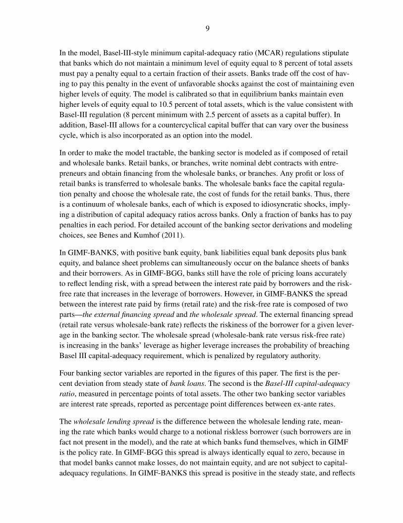
This paper documents the comparative simulation properties of two versions of the Inter-national Monetary Fund’s Global Integrated Monetary and Fiscal Model (GIMF). The firstversion is the original GIMF, with a conventional financial accelerator mechanism that fol-lows Bernanke, Gertler, and Gilchrist (1999) and Christiano, Motto, and Rostagno (2014).The theory of this model, which we will refer to as GIMF-BGG, is documented in Kumhofand others (2010), and its simulation properties in Anderson and others (2013). In this modelbanks, because they write state-contingent lending contracts with their borrowers, make zeroprofits in all states of the world, and therefore do not require equity to protect their deposi-tors against adverse shocks. Therefore, while banks determine the lending spread faced byborrowers, bank equity and bank balance sheets play no meaningful role. The second versionof GIMF, which we will refer to as GIMF-BANKS, is identical to GIMF-BGG in all but thespecification of the banking sector. The theory underlying the banking sector is documentedin Benes and Kumhof (2011). In this model, banks fix their lending rates one period ahead ofthe repayment due-date of the loan, and therefore generally make profits or losses when theeconomy experiences macroeconomic shocks. Because banks also face regulatory constraintsthat represent Basel-III capital-adequacy regulations, bank equity assumes a critical role as ashock absorber, and bank balance sheets become an essential part of the model.

In most of this paper we will compare the GIMF-BGG simulations of Anderson and others(2013) to the corresponding GIMF-BANKS simulations. For a consistent comparison of thetwo models, the paper opts for identical country coverage and calibration as in Anderson andothers (2013), with the exception of the banking sector. The properties of both models areillustrated by showing the response of key macroeconomic variables to different shocks. Thefocus is on the response of U.S. macroeconomic variables to U.S. shocks, because spilloversto other regions of the world are small, and more importantly exhibit only small differencesbetween GIMF-BGG and GIMF-BANKS. The reader who is interested in spillover prop-erties is therefore referred to Anderson and others (2013) for more details. The qualitativeproperties that we show for the U.S. response to U.S. shocks will in general also hold for theresponse of other regions to shocks originating in those regions, but with some differencesthat result from special features in each region, such as different degrees of trade openness,different shares of liquidity-constrained households in the population, or different exchangerate regimes.

Section II contains a short description of GIMF-BGG and GIMF-BANKS, which summarizesKumhof and others (2010) and Benes and Kumhof (2011). Sections III through VI explorethe response of the two models to different types of shocks, specifically fiscal stimulus shocks,aggregate demand shocks, aggregate supply shocks, and financial sector shocks. Section VIIconcludes.

5

II. THE GLOBAL INTEGRATED MONETARY AND FISCAL MODEL (GIMF)

GIMF is a multicountry Dynamic Stochastic General Equilibrium (DSGE) model with opti-mizing behavior by households and firms, and full intertemporal stock-flow accounting. Thereare frictions in the form of nominal rigidities in prices and wages, and real rigidities in con-sumption, investment and imports. Households exhibit non-Ricardian behavior, with finiteplanning horizons among one group of households, and liquidity constraints among the remain-ing group of households.

The assumption of finite planning horizons1 distinguishes GIMF from standard monetaryDSGE models. It implies that steady state net-foreign-asset positions and the steady stateworld real interest rate are endogenously determined by variables that include not only prefer-ences but also the level of government debt and and structure of taxation (distortionary capitaltaxes, for instance). Finite planning horizons together with liquidity constraints generate non-Ricardian behavior in response to both spending-based and revenue-based fiscal measures,which makes the model particularly suitable to analyze fiscal policy questions.2

Asset markets are incomplete in GIMF. All financial contracts last one period. Governmentdebt and bank deposits are only held domestically, are denominated in domestic currency, andare non-contingent. The only assets traded internationally are non-contingent bonds denomi-nated in U.S. dollars. Firms are owned domestically, and firm equity is not traded in domesticfinancial markets. Instead, households receive lump-sum dividend payments.

Firms employ capital and labor to produce tradable and nontradable intermediate goods. Afinancial accelerator mechanism based on Bernanke, Gertler, and Gilchrist (1999) is opera-tive. When banks take over defaulting firms and liquidate their capital, they can only do soat a discount. This implies that banks’ lending rate includes an external financing premium,which varies directly with the leverage (debt-to-equity) ratio of borrowers. Beyond this, thereare important differences between the financial sectors in GIMF-BGG and GIMF-BANKSthat will be discussed in more detail in Section II.C below.

GIMF features multiple regions that encompass the entire world economy. All bilateral tradeflows, and the associated relative prices for each region, are explicitly modeled. The versionused in this paper comprises 5 regions: the United States, the euro area, Japan, emerging Asia(including China), and, as a single entity, remaining countries.

1See Blanchard (1985) for the basic theoretical building blocks, and Kumhof and Laxton (2007, 2013) foranalyses of the fiscal policy implications.

2Coenen and others (2012) show that GIMF fiscal multipliers for temporary shocks are similar to those ofstandard monetary business cycle models.

6

A. Household Sector

There are two types of households, who both consume goods and supply labor. Overlapping-generations (OLG) households smooth consumption over their expected remaining lifetime,or planning horizon, of 20 years, by borrowing and lending in domestic and internationalcredit markets. By contrast, liquidity-constrained (LIQ) households have no access to creditmarkets, and therefore consume their disposable income in every period. Households paydirect taxes on labor income, indirect taxes on consumption spending, and a lump-sum tax,and receive government transfers that are either paid to all households equally, or targetedspecifically to LIQ households.

OLG households save by acquiring domestic government bonds, international U.S. dollarbonds, and deposits in domestic banks. They maximize their lifetime utility subject to theirintertemporal budget constraint. Aggregate OLG consumption is a function of financial wealthand of the present discounted value of after-tax income. The consumption of LIQ households,which are often referred to as rule-of-thumb households in the literature, is equal to their cur-rent net income, so that their marginal propensity to consume out of current income is closeto unity.3 A high proportion of LIQ households in the population therefore implies significantfiscal multipliers from temporary changes to taxes and transfer payments.

For OLG households with finite-planning horizons, a tax cut has a short-run positive effecton demand. Even when the cut is matched with a tax increase in the future that leaves gov-ernment debt unchanged in the long run, the short-run impact remains positive, as the changewill tilt the time profile of consumption toward the present. In effect, OLG households dis-count future tax liabilities at a higher rate than the market rate of interest. Thus, an increase ingovernment debt today represents an increase in their wealth, because a share of the resultinghigher future taxes is payable beyond their planning horizon. If the increase in governmentdebt is permanent, with tax rates rising sufficiently in the long run to stabilize the debt-to-GDP ratio at higher total interest payments, this will raise real interest rates, and crowd outboth real private capital and net foreign assets.

Increases in the real interest rate have a negative effect on consumption, mainly through theirimpact on the discount rate in the expressions for household wealth. Households’ intertem-poral elasticity of substitution in consumption determines the magnitude of the long-runcrowding-out effects of government debt, since it determines the extent to which real inter-est rates have to rise to encourage households to provide the required savings.

3It is not exactly equal to unity due to the presence of consumption taxes.

7

B. Production Sector

Firms, which produce tradable and nontradable intermediate goods, are managed in accor-dance with the preferences of their owners, OLG households. They therefore also have finiteplanning horizons. The main substantive implication of this assumption is the presence of asubstantial equity premium driven by impatience. Firms are subject to real rigidities in laborhiring and investment. They operate in monopolistically competitive output markets, and thusgoods prices contain a markup over marginal cost. Goods prices and wages exhibit nominalrigidities. Exports are priced to the local destination market, and imports are subject to quan-tity adjustment costs. Firms pay capital income taxes to the government, wages and economicprofits (mostly due to markups) to households, and the return to capital to entrepreneurs, whosupply the capital.

Entrepreneurs borrow from banks because their retained earnings do not fully finance invest-ment. If their earnings fall below the minimum required to make the contracted interest pay-ments, banks take over the entrepreneur’s capital stock, and realize its value after deductingbankruptcy monitoring costs.

Final output is produced using public infrastructure (the government capital stock) as aninput, in combination with tradable and nontradable intermediate goods. Therefore, govern-ment capital adds to the productivity of the economy.

C. Financial Sector

GIMF contains a limited menu of financial assets. Government debt and bank loans are non-contingent, are denominated in domestic currency, and are not tradable across borders. OLGhouseholds may, however, issue or purchase internationally tradable U.S.-dollar-denominatedobligations. Unlike in Goodhart and others (2012), debt contract maturity is one period andno maturity mismatch exists on banks’ balance sheets in the model. Firms do not issue trad-able equity, but rather pay out their after-tax cash flow in a lump-sum fashion. Banks pro-vide loans only to entrepreneurs in the home country, for direct spillover implications ofglobal banks, see Kollmann (2013) or Fecht, Grüner, and Hartmann (2012). Neither versionof GIMF features an explicit housing market and housing loans, as in Gurrieri and Iacoviello(2013), for instance.

8

1. Banks in GIMF-BGG

Following Bernanke, Gertler, and Gilchrist (1999), banks write state-contingent lending con-tracts, which ensure zero profits in each state of nature.4 This means that no equity, and nomacro-prudential regulation, are required to protect banks and the wider economy from vul-nerabilities in the banking sector. With zero equity, bank loans equal bank deposits. Balancesheet problems can therefore only arise among banks’ borrowers, entrepreneurs. Banks’ roleis solely to price loans to accurately reflect lending risk, with an optimality condition wherebythe spread between the interest rate paid by borrowers and the risk-free rate increases withthe leverage of borrowers. The reason is that with high leverage, borrowers have less “skin inthe game”, so that negative payoffs to lenders in the event of borrower bankruptcy are larger.Higher average lending rates are therefore needed to guarantee zero profits. For a discussionof technical details of the GIMF-BGG, see Kumhof and others (2010).

2. Banks in GIMF-BANKS

The GIMF-BANKS model follows the model by Benes and Kumhof (2011). In contrast toBernanke, Gertler, and Gilchrist (1999), Christiano, Motto, and Rostagno (2014), or Curdiaand Woodford (2010), the banks have their own non-zero net worth and are exposed to non-diversifiable aggregate risk determined endogenously on the basis of optimal standard nom-inal debt contract. The absence of net worth changes would preclude an analysis of macro-prudential capital-adequacy regulation of bank balance sheets.

Changes in the net worth of banks result mainly from unexpected profit or loss due to thestandard nominal debt contract, which is an important deviation from the standard BGG setupoften found in the literature. The ex-ante contracted interest rate between the bank and theborrower is not state-contingent and cannot be re-set later, for the bank to break even. As aconsequence, an unexpected change in the economy’s fundamentals results either in profit orloss for the bank, impacting its net worth.

The critical factor in determining bank’s choice of capital structure is capital-adequacy reg-ulation. Banks operate under limited liability for its shareholders and hold equity to protectthemselves against the penalties that become due to the regulator (government), should banksviolate capital-adequacy requirements. The capital regulation is not based on a hard-wiredcapital ratio, as in Angeloni and Faia (2009), for instance. Rather, regulation is viewed as asystem of penalties imposed on banks in case they fall below the regulatory minimum. Suchpenalties then create behavioral incentives for banks to choose endogenous regulatory capitalbuffers under uncertainty, an idea first advocated by Milne (2002).

4We emphasize that state-contingent lending contracts have more in common with banks taking an equitystake in firms than with real-world lending, where banks’ payoff is invariant to the state of the world exceptwhen borrowers default.

9

In the model, Basel-III-style minimum capital-adequacy ratio (MCAR) regulations stipulatethat banks which do not maintain a minimum level of equity equal to 8 percent of total assetsmust pay a penalty equal to a certain fraction of their assets. Banks trade off the cost of hav-ing to pay this penalty in the event of unfavorable shocks against the cost of maintaining evenhigher levels of equity. The model is calibrated so that in equilibrium banks maintain evenhigher levels of equity equal to 10.5 percent of total assets, which is the value consistent withBasel-III regulation (8 percent minimum with 2.5 percent of assets as a capital buffer). Inaddition, Basel-III allows for a countercyclical capital buffer that can vary over the businesscycle, which is also incorporated as an option into the model.

In order to make the model tractable, the banking sector is modeled as if composed of retailand wholesale banks. Retail banks, or branches, write nominal debt contracts with entre-preneurs and obtain financing from the wholesale banks, or branches. Any profit or loss ofretail banks is transferred to wholesale banks. The wholesale banks face the capital regula-tion penalty and choose the wholesale rate, the cost of funds for the retail banks. Thus, thereis a continuum of wholesale banks, each of which is exposed to idiosyncratic shocks, imply-ing a distribution of capital adequacy ratios across banks. Only a fraction of banks has to paypenalties in each period. For detailed account of the banking sector derivations and modelingchoices, see Benes and Kumhof (2011).

In GIMF-BANKS, with positive bank equity, bank liabilities equal bank deposits plus bankequity, and balance sheet problems can simultaneously occur on the balance sheets of banksand their borrowers. As in GIMF-BGG, banks still have the role of pricing loans accuratelyto reflect lending risk, with a spread between the interest rate paid by borrowers and the risk-free rate that increases in the leverage of borrowers. However, in GIMF-BANKS the spreadbetween the interest rate paid by firms (retail rate) and the risk-free rate is composed of twoparts—the external financing spread and the wholesale spread. The external financing spread(retail rate versus wholesale-bank rate) reflects the riskiness of the borrower for a given lever-age in the banking sector. The wholesale spread (wholesale-bank rate versus risk-free rate)is increasing in the banks’ leverage as higher leverage increases the probability of breachingBasel III capital-adequacy requirement, which is penalized by regulatory authority.

Four banking sector variables are reported in the figures of this paper. The first is the per-cent deviation from steady state of bank loans. The second is the Basel-III capital-adequacyratio, measured in percentage points of total assets. The other two banking sector variablesare interest rate spreads, reported as percentage point differences between ex-ante rates.

The wholesale lending spread is the difference between the wholesale lending rate, mean-ing the rate which banks would charge to a notional riskless borrower (such borrowers are infact not present in the model), and the rate at which banks fund themselves, which in GIMFis the policy rate. In GIMF-BGG this spread is always identically equal to zero, because inthat model banks cannot make losses, do not maintain equity, and are not subject to capital-adequacy regulations. In GIMF-BANKS this spread is positive in the steady state, and reflects

10

both the likelihood that bank equity drops below the MCAR and the size of the regulatorypenalty that becomes payable if this happens. Furthermore, variations in the wholesale lend-ing spread become an important part of the macroeconomic adjustment mechanism in GIMF-BANKS.

The external financing spread is the difference between the retail lending rate, meaning therate which banks charge to risky borrowers, and the wholesale lending rate. In GIMF-BGGthe retail lending rate is state-contingent, the wholesale lending rate is the policy rate, andthe spread reported in the figures represents the expected retail lending rate minus the whole-sale lending rate. In GIMF-BANKS both the retail and wholesale lending rates are not state-contingent.

The external financing spread needs to be carefully distinguished from the external financingpremium of Bernanke, Gertler, and Gilchrist (1999) and the subsequent literature. The exter-nal financing premium equals the spread over the wholesale lending rate of an average returnover all loans, including the interest received on loans that do not default and the recoveryvalue of the capital seized from firms that do default. Monitoring costs drive a wedge betweenthe previous going-concern value of the capital before bankruptcy and the recovery valueafter bankruptcy. In the steady state this necessitates a positive external financing premiumthat is exactly equal to the recovery losses as a percentage of the value of assets. This notionof the external financing premium, rather than the external financing spread, has predomi-nated in the financial accelerator literature, although unlike the external financing spreadit does not have a clearly identifiable counterpart in the data. We have used this variable toensure backward compatibility of the steady states of GIMF-BGG and GIMF-BANKS. Specif-ically, we have calibrated GIMF-BANKS in such a way that the steady state external financ-ing premium is identical to that used in the calibration of GIMF-BGG in Anderson and others(2013).

The model equations and calibration of GIMF-BGG and GIMF-BANKS are mostly identi-cal, except, of course, for the banking sector, where there are four key differences. First, inGIMF-BGG the zero profit condition of banks has to hold in all states of the world, while inGIMF-BANKS it only has to hold ex ante, with shock realizations generally implying profitsor losses. Second, in GIMF-BANKS loans equal deposits plus equity, while in GIMF-BGGloans equal deposits. Third, in GIMF-BANKS bank equity becomes a new state variablewith an accumulation equation. This implies that, similar to the effects of equity on borrowerbalance sheets, banks become the source of an additional financial accelerator mechanism.Fourth, in GIMF-BGG the lending rate to a notional riskless borrower equals the policy rate,while in GIMF-BANKS the lending rate to the same notional riskless borrower equals thepolicy rate plus a spread that reflects the cost associated with Basel III regulatory require-ments.

In terms of calibration, the equity of entrepreneurs is calibrated to be identical in GIMF-BGGand GIMF-BANKS, at 66 percent of GDP. Bank equity in GIMF-BGG is zero, but it is pos-

11

itive, at 7 percent of GDP, in GIMF-BANKS. In GIMF-BANKS there is therefore additionalrisk-bearing equity in the economy that can help to absorb macroeconomic shocks.

D. International Dimensions

All bilateral trade flows, and the corresponding prices and exchange rates, are explicitly mod-eled in GIMF. Trade flows include exports and imports of both intermediate and final goods,and are calibrated in steady state to match the bilateral flows observed in recent data. Becauseof households’ finite planning horizons, steady-state net-foreign-asset positions, and the steady-state world real interest rate, are determined by the interaction of global saving and invest-ment decisions.

E. Fiscal and Monetary Policy

Fiscal policy is conducted using a variety of expenditure and tax instruments. Governmentspending may take the form of consumption or investment5 spending on goods and services,or of lump-sum transfers, made either to all households or targeted towards LIQ households.Revenue accrues from taxes on labor income and capital income, consumption taxes, lump-sum taxes, and tariffs on imported goods.

The fiscal policy rule ensures that in the long run the government debt-to-GDP ratio con-verges to its target level, while in the short run countercyclical fiscal policy, representing auto-matic stabilizers, is in effect. The rule is implemented through changes in general transfers,but this can be replaced with other tax, transfer or spending instruments if that is consideredmore realistic for a specific region.

The inflation-forecast-based interest rate reaction function of monetary policy varies the gapbetween the actual policy rate and the long-run equilibrium rate to achieve a stable target rateof inflation over time. In the simulations reported in this paper, monetary policy is assumed tooperate normally, without constraints due to the zero lower bound on nominal interest rates.

5Government investment spending augments a public capital stock that enters the economy’s aggregatetechnology. This capital stock depreciates at a fixed rate over time.

12

III. PROPERTIES OF FISCAL STIMULUS SHOCKS

This section studies the simulation properties of GIMF-BGG and GIMF-BANKS in responseto changes in the seven fiscal instruments in GIMF – government consumption, governmentinvestment, general lump-sum transfers, lump-sum transfers targeted to LIQ households, andtaxes on private consumption, labor income and capital income. The simulation experimentsare conducted in the United States block of the model. Unlike in Anderson and others (2013),we will limit the policy experiments to temporary fiscal stimulus measures, specifically tofiscal stimulus that expires after two years, while omitting simulations of permanent fiscalconsolidations. The reason is that for fiscal policy shocks the differences between the twovariants of GIMF are invariably small, and the simulations of temporary measures are suf-ficient to demonstrate that. For the simulations of permanent measures the reader is there-fore referred to Anderson and others (2013) for details. In this and all following subsections,results are reported in terms of deviations from the steady-state baseline.

A. Two-Year Increase in Government Consumption or Government Investment

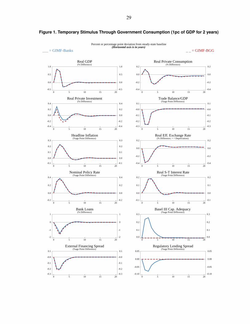
Figures 1 and 2 compare the effects of increasing either U.S. government consumption orU.S. government investment by 1 percentage point of baseline GDP for two years. The increasein government consumption drives up real GDP by slightly less than 1 percent for two years,while headline inflation rises by around a quarter of one percentage point. When the samestimulus measure is performed through government investment, real GDP increases by justover 1 percent after two years, and thereafter stays above baseline for an extended period,with inflation effects similar to the case of government consumption.

Under both types of stimulus, higher government spending increases aggregate demand directly.Since government goods are assumed to be produced using both domestic and imported inputs,there are notable effects in both the domestic and external sectors. The increase in demand fordomestic goods increases marginal cost and prices of domestic goods. In response to risinginflation, the U.S. monetary authority increases the nominal policy interest rate. This leads tohigher real interest rates, which increase the cost of capital, thereby dampening private invest-ment demand and partly offsetting the expansionary effect of the stimulus measure. Higherreal interest rates also reduce the present discounted value of future incomes, in other wordsconsumer wealth, which works to offset the impact of higher incomes on consumption expen-diture. Fiscal policy also operates in a countercyclical fashion. Specifically, automatic fiscalstabilizers operate such that transfers adjust to dampen private demand, especially demand ofLIQ households whose current consumption moves with their current income almost one-for-one. The increase in real interest rates appreciates the U.S. real effective exchange rate. As aresult, the trade balance temporarily deteriorates.

13

What differentiates an increase in government investment from that of an increase in govern-ment consumption is the additional stimulative effect of government investment on the gov-ernment capital stock, which positively affects private sector aggregate productivity and realGDP. The resulting positive productivity and wealth effects account for the much strongerresponses of both investment and consumption.

The differences between GIMF-BGG and GIMF-BANKS in these simulations have their ori-gin in the fact that banks in GIMF-BANKS can make net lending gains or losses that changetheir capital-adequacy ratio, while in GIMF-BGG banks make no net lending gains or losses.Specifically, in GIMF-BANKS the capital-adequacy ratio changes by between 0.25 and 0.30percentage points of total assets in Figures 1 and 2. The reason for the improvement of thecapital-adequacy ratio in GIMF-BANKS is that the increase in demand triggered by fiscalstimulus leads to above-average returns to lending at the previously set lending rate. This per-mits a 7-9 basis points reduction of the wholesale lending spread, which reflects the state ofbanks’ balance sheets. This, by feeding through to the final lending rate, stimulates invest-ment activity. The overall effect, however, is small, because its aggregate demand implica-tions are limited to investment, and because even the differences in investment performanceare not dramatic. As a result, the behavior of GDP under GIMF-BGG and GIMF-BANKS isvery similar.

An additional reason for the small size of the overall effect is the behavior of the externalfinancing spread, which reflects the state of borrowers’ balance sheets. Changes in the exter-nal financing spread partly (but not completely) offset changes in the wholesale lending spread,so that the drop in the overall lending spread is smaller than the drop in the wholesale lendingspread. We will encounter this for several other shocks below. The reason is that the funda-mentals of credit demand in these two models are virtually identical, because the initial stateof bank borrowers is calibrated to be identical across the two models. The market clearinglending rate is determined by the interplay between credit demand and credit supply. Whenthe wholesale lending spread drops, the required drop in the external financing spread is rel-atively lower in GIMF-BANKS than in GIMF-BGG to clear the loan market, to attain essen-tially identical retail rate level.

Figure 3 turns to the question of why the increase in demand triggered by fiscal stimulusleads to above-average returns to lending at the previously set lending rate. To study thisquestion we need to examine the expression of bank loan losses Λ`t in GIMF:6

Λ`t x = r`,t ˇt−1 − qt−1 kt−1retk ,tγt . (1)

In period t − 1, retail lending banks borrowed the funds they lent to entrepreneurs, ˇt−1, atthe nominal wholesale lending rate i`,t−1. Their real ex-post cost of these funds in period tequals ˇt−1 multiplied by the real wholesale lending rate r`,t = i`,t−1/πt , where πt is headline

6An inverted hat above a variable indicates normalization by aggregate productivity. The term x is the econ-omy’s steady state growth rate of productivity. It has no material implications for our analysis.

14

inflation. Therefore, if time t inflation is higher than expected at the time of contracting theloan, banks’ real loan losses will, ceteris paribus, be lower.

The second part of loan losses represents banks’ share γt in the return on the capital put inplace by their borrowers in the previous period, qt−1 kt−1retk ,t , where qt−1 kt−1 is the time t − 1market value of physical capital kt−1, while retk ,t is the financial return on capital betweenperiods t − 1 and t. The latter includes depreciation adjusted capital gains, the user cost ofcapital, and the effects of capital income taxes. Because qt−1 kt−1 is predetermined, the twodeterminants of bank loan losses in this expression are the financial return to capital andbanks’ share in that return. Ceteris paribus, a larger than expected financial return to capitalreduces banks’ loan losses, and so does an increase in banks’ share in that return.

Figure 3 shows a decomposition of the terms in (1) for the stimulus based on governmentspending of Figure 1. Variables with an overbar denote the steady-state value of the variable,to help visualise the decomposition of the loan losses evolution. Our focus is exclusively onperiod 1, the period when the shock hits. This is because profits in all subsequent periodshave to equal zero, as banks can, following the initial shock, adjust their lending rates to takeaccount of the shock. We begin with banks’ share in the return to capital which, strikingly,remains almost completely unchanged on impact. The increase in aggregate demand does ofcourse lead to a significantly higher financial return to capital, but this is almost exactly offsetby a reduction in banks’ share in that return. The reason is the limited liability of banks’ bor-rowers, which means that borrowers and not banks are the residual claimants on the returnsto capital. Firms are more profitable but due to the structure of the nominal debt contractthey repay only what has been agreed. The upside comes from less firms going bankruptthan anticipated. On the funding side, positive inflation surprise redistributes resources fromdepositors to lenders.

We will not repeat the detailed analysis of Figure 3 for all but one of the remaining shocksstudied in this paper. The reason is that for most other shocks the pattern displayed in Figure3 is repeated. The exception is shocks to borrower riskiness, which will be studied in SectionVI.

B. Two-Year Increase in General or Targeted Lump-sum Transfers

Figures 4 and 5 show the effects of an increase in U.S. lump-sum transfers by 1 percent-age point of baseline GDP for two years, either targeted to only LIQ households (Figure 4)or paid equally to all households (Figure 5). Transfers do not feed into aggregate demanddirectly, but indirectly through the effect of household incomes on household spending. Theincrease in general transfers is split between OLG households and LIQ households, based ontheir calibrated share of the total U.S. population (75% and 25%, respectively).

15

When targeted lump-sum transfers are increased, real GDP increases by around 0.4 percent,while inflation rises by around 0.15 percentage points. When general lump-sum transfersare increased, the increases in real GDP and inflation equal only around one quarter of thosemagnitudes.

When temporarily higher transfers are directed only to LIQ households (Figure 4), there is alarger immediate increase in private consumption and aggregate demand, mainly because LIQhouseholds spend all of their current income. The increase in aggregate demand puts upwardpressure on inflation, with the monetary policy response driving up real interest rates. Theincrease in real interest rates, which is considerably more persistent than the fiscal stimulus,due to inflation persistence and central bank interest rate smoothing, puts downward pressureon private investment, which declines as soon as the stimulus expires. Higher interest rates,by increasing the rate at which OLG households discount future incomes, also partly offsetthe impact of higher household incomes on private consumption. In addition, automatic fis-cal stabilizers reduce transfers during the upturn, again partly offsetting the boost to privatedemand. These factors in combination lead to a fiscal multiplier well below unity, at around0.4. The increase in real interest rates appreciates the U.S. real effective exchange rate andleads to a temporary deterioration in the trade balance.

When the temporary increase in transfers is paid equally to all households (Figure 5), theeffects are qualitatively similar, but much smaller, since OLG households can smooth theirconsumption using their access to capital markets. Thus the boost to private consumption, andto aggregate demand, is primarily driven by the transfers to LIQ households, whose increasein income is only one quarter of the case of targeted transfers.

The differences between GIMF-BGG and GIMF-BANKS are, again, quantitatively small.

C. Two-Year Decrease in Taxation

Figures 6, 7 and 8 compare the effects of a reduction in taxation equal to 1 percent of baselineGDP for 2 years, using either consumption taxes, labor income taxes or capital income taxes.All of these tax cuts produce modest GDP gains of 0.25–0.30 percent.

The three different taxes have different transmission channels. Consumption and labor incometax cuts primarily affect households. Since these tax cuts are temporary, their demand effectsare primarily due to LIQ households. But because they also have beneficial supply side effects,by removing distortions, their GDP effects lie between those of targeted and untargeted lump-sum transfers. Finally, capital income tax cuts primarily affect firms.

Lower consumption taxes (Figure 6) directly decrease the price that households pay for con-sumption goods. On the supply side, this reduces the gap between the real wage and the mar-ginal rate of substitution between consumption and leisure, so that households are willing to

16

increase their labor supply. On the demand side, lower after-tax prices of consumption goodsand higher labor supply lead to higher incomes and private consumption for the two yearsof the stimulus. The increase in demand leads to a small increase in CPI inflation (excludingindirect taxes), and thereby of nominal and real interest rates.

Lower labor income taxes (Figure 7) work in a very similar way to lower consumption taxes.On the supply side, they reduce the wedge between the real wage and the marginal rate ofsubstitution in the same way, leading to higher labor supply but also a drop in pre-tax realwages. On the demand side, higher household incomes are now derived from a higher take-home pay for each hour of labor supplied, despite the drop in pre-tax real wages. This againresults in an increase in private consumption, driven primarily by higher consumption of LIQhouseholds. The increase in aggregate demand only partly offsets the downward pressure onpre-tax real wages from increased labor supply, so that inflation drops slightly. The resultingsmall drop in real interest rates implies a stronger performance of investment than for the caseof lower consumption taxes. But the performance of consumption is considerably weaker, dueto the absence of a drop in the after-tax price of consumption goods.

Lower capital income tax rates (Figure 8) raise the after-tax return to capital, which inducesfirms to invest more during the two years of the stimulus. Private consumption also increasesslightly, due to the positive income and wealth effects that follow higher capital investment.Stronger private demand results in slightly higher inflation, and increases in nominal and realinterest rates that, together with countercyclical fiscal policy, partly offset the effects of thestimulus.

Fiscal multipliers are well below unity for tax-based fiscal stimulus measures. The main rea-sons are the lack of a direct demand effect, and the very low marginal propensity of OLGhouseholds to consume the additional income.

In all three cases, the demand boost that follows the tax cuts leads to higher bank profits,increased share of banks’ net worth on assets, and consequently lower wholesale lendingspreads. The effects are smallest for a cut in labor income taxes, since the bank loans are pro-cyclical and bank’s net worth over loans improves only marginally. The effects are largestfor a cut in capital income taxes. However, even for this case the differences between GIMF-BGG and GIMF-BANKS in the behavior of investment and of GDP are small.

IV. PROPERTIES OF DEMAND SHOCKS

This section presents the effects of temporary shocks to private domestic demand in the UnitedStates. We will study two shocks, a shock to the policy interest rate, which is typically groupedwith demand shocks because its primary effect is on aggregate demand, and a combinedshock to private domestic consumption and investment.

17

A. Temporary Increase in the Policy Rate

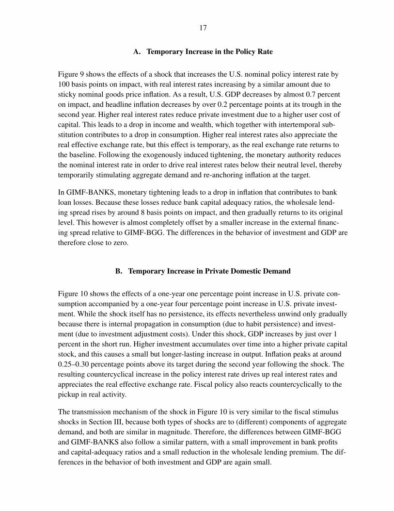
Figure 9 shows the effects of a shock that increases the U.S. nominal policy interest rate by100 basis points on impact, with real interest rates increasing by a similar amount due tosticky nominal goods price inflation. As a result, U.S. GDP decreases by almost 0.7 percenton impact, and headline inflation decreases by over 0.2 percentage points at its trough in thesecond year. Higher real interest rates reduce private investment due to a higher user cost ofcapital. This leads to a drop in income and wealth, which together with intertemporal sub-stitution contributes to a drop in consumption. Higher real interest rates also appreciate thereal effective exchange rate, but this effect is temporary, as the real exchange rate returns tothe baseline. Following the exogenously induced tightening, the monetary authority reducesthe nominal interest rate in order to drive real interest rates below their neutral level, therebytemporarily stimulating aggregate demand and re-anchoring inflation at the target.

In GIMF-BANKS, monetary tightening leads to a drop in inflation that contributes to bankloan losses. Because these losses reduce bank capital adequacy ratios, the wholesale lend-ing spread rises by around 8 basis points on impact, and then gradually returns to its originallevel. This however is almost completely offset by a smaller increase in the external financ-ing spread relative to GIMF-BGG. The differences in the behavior of investment and GDP aretherefore close to zero.

B. Temporary Increase in Private Domestic Demand

Figure 10 shows the effects of a one-year one percentage point increase in U.S. private con-sumption accompanied by a one-year four percentage point increase in U.S. private invest-ment. While the shock itself has no persistence, its effects nevertheless unwind only graduallybecause there is internal propagation in consumption (due to habit persistence) and invest-ment (due to investment adjustment costs). Under this shock, GDP increases by just over 1percent in the short run. Higher investment accumulates over time into a higher private capitalstock, and this causes a small but longer-lasting increase in output. Inflation peaks at around0.25–0.30 percentage points above its target during the second year following the shock. Theresulting countercyclical increase in the policy interest rate drives up real interest rates andappreciates the real effective exchange rate. Fiscal policy also reacts countercyclically to thepickup in real activity.

The transmission mechanism of the shock in Figure 10 is very similar to the fiscal stimulusshocks in Section III, because both types of shocks are to (different) components of aggregatedemand, and both are similar in magnitude. Therefore, the differences between GIMF-BGGand GIMF-BANKS also follow a similar pattern, with a small improvement in bank profitsand capital-adequacy ratios and a small reduction in the wholesale lending premium. The dif-ferences in the behavior of both investment and GDP are again small.

18

V. PROPERTIES OF SUPPLY SHOCKS

This section studies the effects of supply shocks, including a one-off permanent increasein the level, and a persistent increase in the growth rate, of labor-augmenting productivity,one-off permanent reductions in wage markups and price markups, and one-off permanentincreases in tariffs.

A. Productivity Shocks

1. Permanent Increase in the Level of Productivity

Figure 11 shows the effects of a permanent one percent increase in the level of labor aug-menting productivity in both the tradable and nontradable intermediate goods sectors in theUnited States. Higher productivity increases the marginal product of capital, which boostsinvestment, as well as increasing household income and wealth, which boosts private con-sumption. Because the increase in productivity is large and immediate, its disinflationaryeffect initially dominates despite the inflationary effects of higher aggregate demand, but theeffect is not large at around 0.05 percentage points during the first and second years followingthe shock. Nevertheless, the resulting decline in the policy rate, by driving down real interestrates, exerts additional upward pressure on investment and consumption. The real effectiveexchange rate persistently depreciates, reflecting the drop in domestic costs of production.The trade balance goes into a prolonged deficit, due to a boom in investment as the capitalstock permanently adjusts to a higher level commensurate with the higher level of productiv-ity.

For this shock, there is little difference between GIMF-BGG and GIMF-BANKS, again. Thereason is that the spread between retail and deposit rates in both models is very small, giventhe size of the shock. The positive supply shock makes entrepreneurs less risky and more inneed of expanding their borrowing to finance the increase investment activity. In GIMF-BGGthe rate of corporate insolvencies drops more than in GIMF-BANKS, which is consistent withaverage lower external financing spread. Banks are willing to extend the loans to entrepre-neurs and by as a result their loan book expands faster than their net worth, resulting in asmall increase in wholesale lending spread.

2. Persistent Increase in the Growth Rate of Productivity

Figure 12 shows the effects of a ten-year anticipated increase in the growth rate of economy-wide labor-augmenting productivity in the United States. The size of the increase in produc-tivity is calibrated to increase the steady-state level of real GDP each year by just under 0.25

19

percent, which results in an increase in the level of real GDP by the end of ten years of justover 2 percent.

Because the increase in productivity is anticipated, it results in an immediate increase inincome and wealth, and therefore in a sizeable increase in private domestic demand that inlarge part, due to consumption smoothing on the part of OLG households, precedes the actualrealizations of the productivity gains. There are two competing effects on inflation. First, thesuccessive increases in productivity put downward pressure on marginal cost and thus onprices, but this effect is gradual. Second, the increase in aggregate demand puts immediateupward pressure on prices. This second effect dominates during the transition, with headlineinflation increasing, albeit modestly, by just over 0.15 percentage points at the peak in years3–5. Countercyclical monetary policy increases real interest rates by around 20 basis pointsat the peak and appreciates the real exchange rate on impact, accompanied by a trade balancedeficit during a lengthy transition. In the long run, however, the real effective exchange ratedepreciates in order to permanently increase external demand for the increased U.S. output.

The differences between GIMF-BGG and GIMF-BANKS are again small. Anticipated pro-ductivity growth shocks share many characteristics with demand shocks, as evidenced bythe behavior of inflation. We therefore observe, as we have previously observed for demandshocks, that banks make lending profits, improve their capital-adequacy ratio, and lowerthe wholesale lending spread. But the effect on the latter is very small, at 2 basis points onimpact, and the movement in the external financing spread partly offsets this. As a result, thebehavior of GDP is indistinguishable between the two models.

B. Permanent Drop in Wage Markups

Figure 13 shows the effects of a permanent increase in the degree of U.S. labor market com-petition that reduces the wage markup by five percentage points. Firms respond to lower wagemarkups by increasing hiring and investment. The permanent increase in production gener-ates an increase in aggregate income and wealth, which leads to higher consumption. In thelong run, real GDP increases by almost 1.5 percent, accompanied by mild disinflationarypressures and by a mild drop in policy and real interest rates that stimulates additional out-put gains, directly and through a depreciation of the real exchange rate. Similar to the caseof productivity shocks, the real exchange rate remains depreciated in the long run, in orderto permanently increase external demand for the increased U.S. output. Similar to the resultsfor productivity shocks, the differences between GIMF-BGG and GIMF-BANKS for wagemarkup shocks are small.

20

C. Permanent Drop in Price Markups

Figure 14 shows the effects of a permanent increase in the degree of U.S. goods market com-petition that reduces the price markup over marginal cost in the tradable and nontradablegoods sectors by five percentage points. Firms respond to greater goods market competi-tion by increasing hiring and investment. The permanent increase in production generatesan increase in aggregate income and wealth, which implies higher consumption. The expan-sion in the economy’s supply capacity raises real GDP by more than 5 percent in the longrun. Despite the downward pressure on price inflation from reduced price markups, alongthe adjustment path to the new equilibrium overall CPI inflation rises by almost 0.4 percent-age points. This is because demand effects are initially very strong, most importantly due toan investment surge that brings the capital stock to a permanently higher level that is consis-tent with reduced monopolistic distortions in the goods market. In response to the increasein inflation, policy and real interest rates rise to return inflation to target. Similar to the caseof productivity shocks, the real exchange rate depreciates in the long run, in order to per-manently increase external demand for the increased U.S. output. The differences betweenGIMF-BGG and GIMF-BANKS are again small. The effects of this shock on the financialsector are expansionary due to the behavior of inflation.

D. Permanent Increase in Tariffs

Figure 15 shows the effects of a permanent, ten percentage point increase in U.S. tariffs onimports from all other regions. Because this increases supply-side distortions in the economy,GDP permanently decreases by around 1 percent, with most of the drop taking place over thefirst two years, while private investment declines by 2 percent in the short run, and by around1.5 percent in the long run. Consumption increases strongly as additional income from tar-iffs is distributed to households via permanently higher general transfers, which increasesLIQ consumption due to higher incomes and OLG consumption due to higher wealth. Thelong-run increase in consumption is around 0.7 percent. Headline inflation increases onlymarginally in the short run, as a large nominal appreciation offsets the increase in importprices due to higher tariffs. Because tariffs raise the relative price of imports, import vol-umes decline. This is accompanied by a real appreciation that reduces foreign demand forU.S. exports, thereby keeping the trade balance approximately in balance, and maintainingthe desired level of net foreign assets.

The differences between GIMF-BGG and GIMF-BANKS are once more small. On impactbanks make small losses. Thereafter, the effects of the shock on real activity and thus onlending are permanent, while banks manage to replace lost equity fairly quickly. As a result,beyond the first two years bank capital-adequacy ratios are improved, and wholesale lendingspreads reduced.

21

VI. PROPERTIES OF FINANCIAL SECTOR SHOCKS

This section presents the effects of a number of shocks to the U.S. financial sector. First, as inAnderson and others (2013), we simulate a temporary increase in borrower riskiness, undertwo alternative assumptions, an equal impact effect on the external financing spread and anequal shock size. Because shocks to borrower riskiness are present in both GIMF-BGG andGIMF-BANKS, these simulations can be performed as a comparison across the two models,as in all other figures up to this point. Second, we simulate the effects of different settings formacroprudential policy, specifically for minimum capital-adequacy ratios (MCAR). Becausethese are only present in GIMF-BANKS, the simulations compare different versions of thatmodel. One simulation subjects the economy to a shock to borrower riskiness, under the alter-native assumptions of fixed or countercyclical MCAR. Another simulation studies the effectsof a permanent increase in MCAR, under the alternative assumptions of immediate or gradualimplementation.

A. Temporary Increase in Borrower Riskiness

1. Equal Impact Effect on External Financing Spread

Figure 16 shows the effects of a temporary but persistent increase in the riskiness of U.S. cor-porate borrowers. In this simulation the shock sizes in GIMF-BGG and GIMF-BANKS arechosen such that on impact external financing spreads increase by 1 percentage point in bothmodels.

In both versions of GIMF, the main effect of higher external financing spreads is to reduceinvestment and the capital stock. The resulting loss in household income and wealth alsodepresses consumption, despite a reduction in the real risk-free interest rate as the monetaryauthority responds to lower inflation. The trade balance improves modestly, and real GDPdeclines.

There are more notable differences between GIMF-BGG and GIMF-BANKS in this simu-lation. In GIMF-BANKS, the sizeable increase in borrower riskiness leads to much higherloan defaults than originally anticipated by banks, and thus to sizeable lending losses thatreduce the average capital adequacy ratio by a full two percentage points, that is from 10.5percent in the baseline to 8.5 percent following the shock. Because actual capital-adequacyratios of individual banks are heterogeneous across institutions, this implies that many banksnow either violate the MCAR of 8 percent, or are very close to doing so. They therefore rushto rebuild their equity buffers, by raising the wholesale lending spread by over 70 basis pointson impact and thereby quickly increasing their profits. Given that the external financing spreadhas been normalized here to increase by 100 basis points on impact in both models, the real

22

lending rate in GIMF-BANKS therefore increases by an additional 70 basis points. The behav-ior of bank loans is consequently also very different, with a smooth and modest decrease inloans in GIMF-BGG, but a drop in loans of almost 3 percent on impact in GIMF-BANKS.Given the greater increase in real lending rates and the larger decline in the volume of lend-ing in GIMF-BANKS, the effects of this shock on the real economy are also larger, with GDP,consumption and investment all contracting by roughly twice as much as in GIMF-BGG.

Figure 17 turns to the question of why the increase in borrower riskiness leads to below-average returns to lending at the previously set lending rate, and thus to losses and a precip-itous decline in capital-adequacy ratios. To study this we need to again examine equation (1).First, the real ex-post cost of bank wholesale borrowing r`,t ˇt−1 increases, because followingthe shock inflation is lower than expected at the time of contracting the loan. However, giventhe very small change in inflation, this effect is negligible in size. Second, and more impor-tantly, banks’ income from lending qt−1 kt−1retk ,tγt decreases, which accounts for close to100 percent of loan losses. The reason is that the increase in borrower riskiness leads to a sig-nificantly lower financial return to capital retk ,tqt−1 kt−1, and unlike for all other shocks stud-ied so far, banks’ share in that return γt does not increase in an offsetting fashion, but ratherremains approximately constant. To understand this, we need to consider the formula for theex-post cutoff productivity level ωt below which borrowers default. This is given by

ωt =rr,t ˇt−1

qt−1 kt−1retk ,t, (2)

where rr,t is the real retail lending rate. The denominator of this expression, except for retk ,t ,is predetermined. This means that the cutoff productivity level ωt moves inversely with thefinancial return to capital retk ,tqt−1 kt−1. Furthermore, it can be shown that, for a given dis-tribution over borrower productivity levels, banks’ share γt in the financial return to capitalincreases approximately one-for-one with the cutoff productivity level ωt , and therefore alsomoves inversely with the financial return to capital retk ,tqt−1 kt−1. This implies that the prod-uct qt−1 kt−1retk ,tγt would ordinarily remain close to constant when the financial return tocapital changes, thereby keeping loan losses from this source small. This is in fact what wehave observed for all other shocks. However, this no longer holds when the distribution overborrower productivity levels itself changes, and that is of course the very definition of bor-rower riskiness shocks. Specifically, when borrower riskiness increases, banks experiencehigher defaults at the same cutoff productivity level ωt , thereby reducing banks’ share γt inthe financial return to capital. In our simulation this downward pressure on γt approximatelyoffsets the upward pressure due to a lower financial return to capital, leaving γt approximatelyunchanged and thereby accounting for large loan losses.

23

2. Equal Size of Shock to Borrower Riskiness

Figure 18 again simulates shocks to borrower riskiness, but in this case the size of the shocks,rather than the size of the increase in the external financing spread, is assumed to be equalacross models. The size of the shocks is chosen to equal the shock in GIMF-BGG in Figure16. The impulse responses for GIMF-BGG in Figure 18 are therefore identical to those inFigure 16. With this normalization we observe significantly smaller differences in the realeffects of the shocks.

The reason is the behavior of spreads. In GIMF-BANKS, the wholesale lending spread risesby almost 50 basis points on impact, and ceteris paribus this significantly reduces the leverageof corporate borrowers. We have already seen this in the behavior of bank loans in Figure 16,and encounter it again in Figure 18. Because bank loans drop by far more in GIMF-BANKS,the external financing spread is significantly lower, which offsets the effect of the higherwholesale lending spread on overall lending rates. The offset is not complete, so that differ-ences remain between overall lending rates. But the differences in the behavior of investment,consumption and GDP are now far smaller than in Figure 16. Essentially, in Figure 16, tocompensate for the offset evident in Figure 18, shocks to borrower riskiness under GIMF-BANKS had to be much larger to generate an identical external financing spread. It is thisdifference in shock sizes that accounted for the major part of the large differences betweenGIMF-BANKS and GIMF-BGG.

B. Shocks to Macroprudential Policy Settings in GIMF-BANKS

1. Fixed versus Countercyclical MCAR

In Figure 19 we simulate a shock to the external financing spread in GIMF-BANKS, withthe size of the shock equal to 100 basis points on impact, as in Figure 16. The assumptionunderlying the blue solid line, labelled “Fixed MCAR”, is that the MCAR is held constant at8 percent of total assets. This simulation is therefore identical to the solid line in Figure 16.The assumption underlying the red dashed line, labelled “Countercyclical MCAR”, is that theMCAR is equal to that same constant plus a feedback term that is increasing in the percentagedeviation of loans from their initial value.

In both simulations banks’ actual capital-adequacy ratio drops by around two percentagepoints on impact, due to the loan losses that follow contractionary shocks to borrower riski-ness. With fixed MCAR, this puts a lot of banks below or near the point where they have tostart paying penalties. This triggers a steep increase in the wholesale lending spread of around70 basis points, as banks start to rebuild lost equity. Taken together with the increase in theexternal financing spread, which reflects the elevated riskiness of borrowers, this causes asteep initial contraction of investment, and therefore also of GDP.

24

On the other hand, with countercyclical MCAR, the regulator responds to a reduced lend-ing volume by temporarily lowering the MCAR, so that banks can rebuild their lost equityover time instead of having to do so immediately. As a result the wholesale lending spreadincreases far less dramatically, while the increase in the external financing spread is approxi-mately the same as under fixed MCAR. Overall lending rates therefore increase by far less,and as a result the impact effect of the shock is only about half as large as under the fixedMCAR assumption, and thereafter smoothed over time.

GIMF-BANKS therefore contains additional lessons for policy that could not be obtainedusing GIMF-BGG, because in the latter bank equity, and a meaningful role of bank balancesheets, is absent. It should be noted, that the model does not consider the possibility thatthe regulation may push activity and associated risks into the shadow banking system, as inKashyap, Berner, and Goodhart (2011), for instance.

2. Immediate versus Gradual Increase in MCAR

Figure 20 simulates an increase in the fixed component, rather than in the countercyclicalcomponent, of capital-adequacy regulations. Specifically, this figure assumes that the MCARitself is permanently raised from its original value of 8 percent of total assets to a new steadystate value of 10 percent of total assets. The blue solid line assumes that this increase becomesmandatory immediately, while the red dashed line assumes that the MCAR is gradually, andlinearly, increased over a period of five years.

Under the immediate increase of the MCAR, banks that were previously solidly capitalizedsuddenly find that they are close to or below the new MCAR. They therefore rush to quicklybuild up additional equity, by raising the wholesale lending spread rapidly by almost 90 basispoints on impact. This higher spread, despite a simultaneous drop in the volume of lending,makes borrowers less creditworthy, and therefore also increases the external financing spread,by just over 10 basis points. This adds up to a roughly 100 basis points increase in lendingspreads, which is only very partially buffered by a 20 basis points reduction in the policyrate. As a result, there is a small but significant contraction of GDP by around 0.3 percenton impact, while the long-run contraction of GDP equals only around 0.1 percent. The fasterattainment of a higher capital ratio therefore comes at the cost of slightly more volatile out-put.

Under the gradual increase in MCAR this is smoothed. Now banks have more time to buildup additional equity, and as a result the wholesale lending spread increases more modestly,and without spiking on impact. The external financing spread barely increases on impactand then quickly declines. The much smoother behavior of real lending rates is reflected ina much smoother behavior of the real economy.

25

We also observe interesting long-run effects of higher MCAR. The wholesale lending spreadincreases by 8 basis points, as banks are permanently obliged to accumulate additional earn-ings in order to maintain a higher capital buffer. This however has the side effect of reducingthe long-run volume of bank loans by around 0.5 percent. Because this implies permanentlylower borrower leverage, the external financing spread is permanently lower by 2 basis points,which partly offsets the increase in the wholesale lending spread. The final effect on real GDPis modest, there is an approximately 0.1 percent contraction.

VII. CONCLUSION

This paper has studied the comparative simulation properties of the two versions of the GIMFmodel. The first is GIMF with a conventional financial accelerator, referred to as GIMF-BGG,which has been used at the IMF for policy and scenario analysis since 2008, and whose sim-ulation properties have been extensively studied in Anderson and others (2013). In this modelbanks play an important role in pricing risky loans, but their balance sheets do not play animportant role, principally because banks write state-contingent lending contracts wherebythey make zero profits in all states of nature, and therefore do not require equity to protecttheir depositors against adverse shocks. State-contingent lending contracts do serve to greatlysimplify financial accelerator models. But their drawback is a lack of realism, as in real-worldlending banks’ payoff is invariant to the state of nature except when borrowers default. In thatworld bank balance sheets are of critical importance, and this importance has been widelyacknowledged following the financial crisis that triggered the Great Recession. The secondversion of GIMF, referred to as GIMF-BANKS, therefore adopts a different specificationof the banking sector, while remaining identical to GIMF-BGG in all other respects. In thismodel banks cannot write fully state-contingent lending contracts, and as a result generallymake profits or losses when the economy experiences macroeconomic shocks. Because banksalso face regulatory constraints that represent Basel-III capital-adequacy regulations, bankequity assumes a critical role as a shock absorber, and bank balance sheets become an essen-tial part of the model.

The simulation results presented in this paper have taken the form of contrasting the proper-ties of GIMF-BGG and GIMF-BANKS, and also to explore some new properties of macro-prudential regulation that are only present in GIMF-BANKS. The main results are as follows.First, following standard fiscal, demand and supply shocks, the properties of GIMF-BGG andGIMF-BANKS are very similar. The reason is that, for a given distribution over borrowerproductivity levels, meaning in the absence of financial shocks, banks’ net loan losses remainsmall. Second, following financial shocks, meaning when the distribution over borrower pro-ductivity levels itself changes, there are notable differences in the properties of GIMF-BGGand GIMF-BANKS. Taking as an example a contractionary shock to borrower riskiness, thereason is that in this case not only do borrowers experience a reduction in the return on their

26

projects, in addition banks experience a reduction, ceteris paribus, in their share of the returnon those projects. This causes loan losses and a deterioration in regulatory capital-adequacyratios, in response to which banks will tend to increase lending spreads for all borrowers,including riskless ones. This mechanism is absent in GIMF-BGG, which therefore exhibitssubstantially smaller effects of contractionary financial shocks. Third, GIMF-BANKS canalso be used to study an additional set of shocks to macroprudential policy instruments thatare absent in GIMF-BGG. This can potentially generate valuable insights for policy.

27

REFERENCES

Anderson, D., Hunt, B., Kortelainen, M., Kumhof, M., Laxton, D., Muir, D., Mursula, S.and Snudden, S. (2013), “Getting to Know GIMF: The Simulation Properties of theGlobal Integrated Monetary and Fiscal Model”, IMF Working Paper Series, WP/13/55,available at http://www.imf.org/external/pubs/cat/longres.aspx?sk=40357.0.

Angeloni, I. and Faia, E. (2009), “A Tale of Two Policies: Prudential Regulation and Mone-tary Policy with Fragile Banks”, IMF The Kiel Institute for the World Economy Work-ing Paper Series, No. 1569

Benes, J. and Kumhof, M. (2011), “Risky Bank Lending and Optimal CapitalAdequacy Regulation”, IMF Working Paper Series, WP/11/130, available athttp://www.imf.org/external/pubs/cat/longres.aspx?sk=24900.0.

Bernanke, B.S., Gertler, M. and Gilchrist, S. (1999), “The Financial Accelerator in a Quan-titative Business Cycle Framework”, in: John B. Taylor and Michael Woodford, eds.,Handbook of Macroeconomics, Volume 1C. Amsterdam: Elsevier.

Blanchard, O.J. (1985), “Debt, Deficits, and Finite Horizons”, Journal of Political Economy,93, 223-247.

Christiano, L., Motto, R. and Rostagno, M. (2010), “Financial Factors in Economic Fluctua-tions”, ECB Working Paper Series, No. 1192.

Christiano, L., Motto, R. and Rostagno, M. (2014), “Risk Shocks”, American EconomicReview, 104(1), 27-65.

Coenen, G., C. Erceg, C. Freedman, D. Furceri, M. Kumhof, R. Lalonde, D. Laxton, J.Lindé, A. Mourougane, D. Muir, S. Mursula, J. Roberts, W. Roeger, C. de Resende,S. Snudden, M. Trabandt, J. in‘t Veld (2012), “Effects of Fiscal Stimulus in StructuralModels”, American Economic Journal: Macroeconomics, 4(1), 22-68.

Curdia, V. and Woodford, M. (2010), “Credit Spreads and Monetary Policy, Journal ofMoney, Credit, and Banking, 24(6), 3-35.

Fecht, F., Grüner, H.P. and Hartmann, P. (2012), “Financial Integration, specialization, andsystemic risk”, Journal of International Economics, 88, 150-161.

Gerali, A., Neri, S., Sessa, L. and Signoretti, E. (2010), “A Tale of Credit and Banking in aDSGE Model of the Euro Area”, Bank of Italy Working Paper Series, No. 740

28

Gertler, M. and Karadi, P. (2011), “A Model of Unconventional Monetary Policy, Journal ofMonetary Economics, 58, 17-34.

Goodhart, Ch.A.E., Kashyap, A.K., Tsomocos, D.P. and A.P. Vardoulakis (2012), “FinancialRegulation in General Equilibrium”, NBER Working Paper Series, WP 17909, avail-able at http://www.nber.org/papers/w17909.pdf.

Guerrieri, L. and Iacoviello, M. (2013), “Collateral Constraints and Macroeconomic Asym-metries”, International Finance Discussion Papers No.1082, Board of Governors of theFederal Reserve System

Kashyap, A.K., Berner, R. and Ch.A.E. Goodhart (2011), “The Macroprudential Toolkit”,IMF Economic Review, 59(2), 145-161.

Kollmann, R. (2013), “Global Banks, Financial Shocks, and International Business Cycles:Evidence from an Estimated Model, Journal of Money, Credit, and Banking, 45(2),159-195.

Kumhof, M. and D. Laxton (2007), “A Party Without a Hangover? On the Effectsof U.S. Fiscal Deficits”, IMF Working Paper Series, WP/07/202, available athttp://www.imf.org/external/pubs/ft/wp/2007/wp07202.pdf.

Kumhof, M. and D. Laxton (2013), “Fiscal Deficits and Current Account Deficits,” Journalof Economic Dynamics and Control, 37(10), 2062-2082.

Kumhof, M., D. Laxton, D. Muir and S. Mursula (2010), “The Global Integrated MonetaryFiscal Model (GIMF) - Theoretical Structure”, IMF Working Paper Series, WP/10/34,available at http://www.imf.org/external/pubs/cat/longres.cfm?sk=23615.0.

Milne, A. (2002), “Bank Capital Regulation as an Incentive Mechanism: Implications forPortfolio Choice”, Journal of Banking and Finance, 26(1),1–23

29

Figure 1. Temporary Stimulus Through Government Consumption (1pc of GDP for 2 years)

Percent or percentage point deviation from steady-state baseline(Horizontal axis is in years)

___ = GIMF-Banks _ _ = GIMF-BGG

-0.5

0.0

0.5

1.0

-0.5

0.0

0.5

1.0

0 5 10 15 20

Real GDP(% Difference)

-0.4

-0.2

0.0

0.2

-0.4

-0.2

0.0

0.2

0 5 10 15 20

Real Private Consumption(% Difference)

-0.4

-0.2

0.0

0.2

0.4

-0.4

-0.2

0.0

0.2

0.4

0 5 10 15 20

Real Private Investment(% Difference)

-0.3

-0.2

-0.1

-0.0

0.1

-0.3

-0.2

-0.1

-0.0

0.1

0 5 10 15 20

Trade Balance/GDP(%age Point Difference)

-0.1

0.0

0.1

0.2

0.3

-0.1

0.0

0.1

0.2

0.3

0 5 10 15 20

Headline Inflation(%age Point Difference)

-0.4

-0.2

0.0

0.2

-0.4

-0.2

0.0

0.2

0 5 10 15 20

Real Eff. Exchange Rate(% Difference; + = Depreciation)

-0.2

0.0

0.2

0.4

-0.2

0.0

0.2

0.4

0 5 10 15 20

Nominal Policy Rate(%age Point Difference)

-0.1

0.0

0.1

0.2

-0.1

0.0

0.1

0.2

0 5 10 15 20

Real S-T Interest Rate(%age Point Difference)

-2

-1

0

1

-2

-1

0

1

0 5 10 15 20

Bank Loans(% Difference)

0.0

0.1

0.2

0.3

0.0

0.1

0.2

0.3

0 5 10 15 20

Basel III Cap. Adequacy (%age Point Difference)

-0.3

-0.2

-0.1

-0.0

0.1

-0.3

-0.2

-0.1

-0.0

0.1

0 5 10 15 20

External Financing Spread(%age Point Difference)

-0.10

-0.05

0.00

0.05

-0.10

-0.05

0.00

0.05

0 5 10 15 20

Regulatory Lending Spread(%age Point Difference)

30

Figure 2. Temporary Stimulus Through Government Investment (1pc of GDP for 2 years)

Percent or percentage point deviation from steady-state baseline(Horizontal axis is in years)

___ = GIMF-Banks _ _ = GIMF-BGG

-0.5

0.0

0.5

1.0

1.5

-0.5

0.0

0.5

1.0

1.5

0 5 10 15 20

Real GDP(% Difference)

-0.2

0.0

0.2

0.4

0.6

-0.2

0.0

0.2

0.4

0.6

0 5 10 15 20

Real Private Consumption(% Difference)

0.0

0.2

0.4

0.6

0.8

0.0

0.2

0.4

0.6

0.8

0 5 10 15 20

Real Private Investment(% Difference)

-0.3

-0.2

-0.1

-0.0

0.1

-0.3

-0.2

-0.1

-0.0

0.1

0 5 10 15 20

Trade Balance/GDP(%age Point Difference)

-0.1

0.0

0.1

0.2

0.3

-0.1

0.0

0.1

0.2

0.3

0 5 10 15 20

Headline Inflation(%age Point Difference)

-0.2

0.0

0.2

0.4

-0.2

0.0

0.2

0.4

0 5 10 15 20

Real Eff. Exchange Rate(% Difference; + = Depreciation)

-0.2

0.0

0.2

0.4

-0.2

0.0

0.2

0.4

0 5 10 15 20

Nominal Policy Rate(%age Point Difference)

-0.1

0.0

0.1

0.2

-0.1

0.0

0.1

0.2

0 5 10 15 20

Real S-T Interest Rate(%age Point Difference)

-2

-1

0

1

-2

-1

0

1

0 5 10 15 20

Bank Loans(% Difference)

-0.2

0.0

0.2

0.4

-0.2

0.0

0.2

0.4

0 5 10 15 20

Basel III Cap. Adequacy (%age Point Difference)

-0.3

-0.2

-0.1

-0.0

0.1

-0.3

-0.2

-0.1

-0.0

0.1

0 5 10 15 20

External Financing Spread(%age Point Difference)

-0.10

-0.05

0.00

0.05

-0.10

-0.05

0.00

0.05

0 5 10 15 20

Regulatory Lending Spread(%age Point Difference)

31

Figure 3. Temporary Stimulus Through Government Consumption - Bank Loan Losses

Λ`t

gdpΛ`t¯

-0.08

-0.06

-0.04

-0.02

0.00

0.02

-0.08

-0.06

-0.04

-0.02

0.00

0.02

0 1 2 3 4 5 6 7 8 9 10

(%age Point Difference)

-0.20

-0.15

-0.10

-0.05

0.00

0.05

-0.20

-0.15

-0.10

-0.05

0.00

0.05

0 1 2 3 4 5 6 7 8 9 10

(%age Point Difference)

r`,t ˇt−1

gdpqt−1 kt−1retk ,tγt

gdp

-0.5

-0.4

-0.3

-0.2

-0.1

0.0

0.1

-0.5

-0.4

-0.3

-0.2

-0.1

0.0

0.1

0 1 2 3 4 5 6 7 8 9 10

(%age Point Difference)

-0.5

-0.4

-0.3

-0.2

-0.1

0.0

0.1

-0.5

-0.4

-0.3

-0.2

-0.1

0.0

0.1

0 1 2 3 4 5 6 7 8 9 10

(%age Point Difference)

qt−1 kt−1retk ,t γgdp

qt−1 kt−1retkγtgdp

-0.2

-0.1

0.0

0.1

0.2

0.3

0.4

-0.2

-0.1

0.0

0.1

0.2

0.3

0.4

0 1 2 3 4 5 6 7 8 9 10

(%age Point Difference)

-0.5

-0.4

-0.3

-0.2

-0.1

0.0

0.1

-0.5

-0.4

-0.3

-0.2

-0.1

0.0

0.1

0 1 2 3 4 5 6 7 8 9 10

(%age Point Difference)

32

Figure 4. Temporary Stimulus Through Targeted Transfers (1pc of GDP for 2 years)

Percent or percentage point deviation from steady-state baseline(Horizontal axis is in years)

___ = GIMF-Banks _ _ = GIMF-BGG

-0.2

0.0

0.2

0.4

0.6

-0.2

0.0

0.2

0.4

0.6

0 5 10 15 20

Real GDP(% Difference)

-0.5

0.0

0.5

1.0

1.5

-0.5

0.0

0.5

1.0

1.5

0 5 10 15 20

Real Private Consumption(% Difference)

-0.4

-0.2

0.0

0.2

-0.4

-0.2

0.0

0.2

0 5 10 15 20

Real Private Investment(% Difference)

-0.2

-0.1

0.0

0.1

-0.2

-0.1

0.0

0.1

0 5 10 15 20

Trade Balance/GDP(%age Point Difference)

-0.05

0.00

0.05

0.10

0.15

-0.05

0.00

0.05

0.10

0.15

0 5 10 15 20

Headline Inflation(%age Point Difference)

-0.3

-0.2

-0.1

-0.0

0.1

-0.3

-0.2

-0.1

-0.0

0.1

0 5 10 15 20

Real Eff. Exchange Rate(% Difference; + = Depreciation)

-0.1

0.0

0.1

0.2

0.3

-0.1

0.0

0.1

0.2

0.3

0 5 10 15 20

Nominal Policy Rate(%age Point Difference)

-0.05

0.00

0.05

0.10

0.15

-0.05

0.00

0.05

0.10

0.15

0 5 10 15 20

Real S-T Interest Rate(%age Point Difference)

-1.0

-0.5

0.0

0.5

-1.0

-0.5

0.0

0.5

0 5 10 15 20

Bank Loans(% Difference)

0.00

0.05

0.10

0.15

0.00

0.05

0.10

0.15

0 5 10 15 20

Basel III Cap. Adequacy (%age Point Difference)

-0.15

-0.10

-0.05

-0.00

0.05

-0.15

-0.10

-0.05

-0.00

0.05

0 5 10 15 20

External Financing Spread(%age Point Difference)

-0.04

-0.02

0.00

0.02

-0.04

-0.02

0.00

0.02

0 5 10 15 20

Regulatory Lending Spread(%age Point Difference)

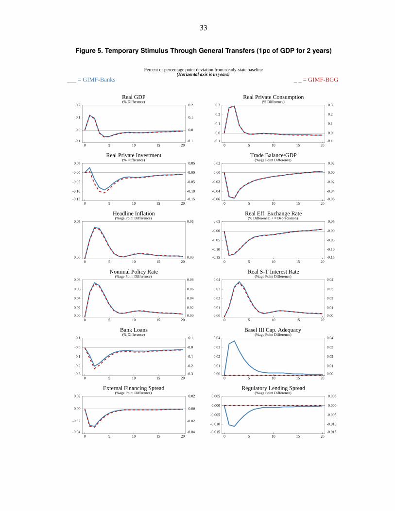
33

Figure 5. Temporary Stimulus Through General Transfers (1pc of GDP for 2 years)

Percent or percentage point deviation from steady-state baseline(Horizontal axis is in years)

___ = GIMF-Banks _ _ = GIMF-BGG

-0.1

0.0

0.1

0.2

-0.1

0.0

0.1

0.2

0 5 10 15 20

Real GDP(% Difference)

-0.1

0.0

0.1

0.2

0.3

-0.1

0.0

0.1

0.2

0.3

0 5 10 15 20

Real Private Consumption(% Difference)

-0.15

-0.10

-0.05

-0.00

0.05

-0.15

-0.10

-0.05

-0.00

0.05

0 5 10 15 20

Real Private Investment(% Difference)

-0.06

-0.04

-0.02

0.00

0.02

-0.06

-0.04

-0.02

0.00

0.02

0 5 10 15 20

Trade Balance/GDP(%age Point Difference)

0.00

0.05

0.00

0.05

0 5 10 15 20

Headline Inflation(%age Point Difference)

-0.15

-0.10

-0.05

-0.00

0.05

-0.15

-0.10

-0.05

-0.00

0.05

0 5 10 15 20

Real Eff. Exchange Rate(% Difference; + = Depreciation)

0.00

0.02

0.04

0.06

0.08

0.00

0.02

0.04

0.06

0.08

0 5 10 15 20

Nominal Policy Rate(%age Point Difference)

0.00

0.01

0.02

0.03

0.04

0.00

0.01

0.02

0.03

0.04

0 5 10 15 20

Real S-T Interest Rate(%age Point Difference)

-0.3

-0.2

-0.1

-0.0

0.1

-0.3

-0.2

-0.1

-0.0

0.1

0 5 10 15 20

Bank Loans(% Difference)

0.00

0.01

0.02

0.03

0.04

0.00

0.01

0.02

0.03

0.04

0 5 10 15 20

Basel III Cap. Adequacy (%age Point Difference)

-0.04

-0.02

0.00

0.02

-0.04

-0.02

0.00

0.02

0 5 10 15 20

External Financing Spread(%age Point Difference)

-0.015

-0.010

-0.005

0.000

0.005

-0.015

-0.010

-0.005

0.000

0.005

0 5 10 15 20

Regulatory Lending Spread(%age Point Difference)

34

Figure 6. Temporary Stimulus Through Lower Consumption Taxes (1pc of GDP for 2 years)

Percent or percentage point deviation from steady-state baseline(Horizontal axis is in years)

___ = GIMF-Banks _ _ = GIMF-BGG

-0.2

0.0

0.2

0.4

-0.2

0.0

0.2

0.4

0 5 10 15 20

Real GDP(% Difference)

-0.5

0.0

0.5

1.0

-0.5

0.0

0.5

1.0

0 5 10 15 20

Real Private Consumption(% Difference)

-0.2

-0.1

0.0

0.1

0.2

-0.2

-0.1

0.0

0.1

0.2

0 5 10 15 20

Real Private Investment(% Difference)

-0.15

-0.10

-0.05

-0.00

0.05

-0.15

-0.10

-0.05

-0.00

0.05

0 5 10 15 20

Trade Balance/GDP(%age Point Difference)

-0.05

0.00

0.05

0.10

-0.05

0.00

0.05

0.10

0 5 10 15 20

CPI Inflation excl. Indirect Taxes(%age Point Difference)

-0.3

-0.2

-0.1

-0.0

0.1

-0.3

-0.2

-0.1

-0.0

0.1

0 5 10 15 20

Real Eff. Exchange Rate(% Difference; + = Depreciation)

0.00

0.05

0.10

0.15

0.20

0.00

0.05

0.10

0.15

0.20

0 5 10 15 20

Nominal Policy Rate(%age Point Difference)

0.00

0.05

0.10

0.00

0.05

0.10

0 5 10 15 20

Real S-T Interest Rate(%age Point Difference)

-0.6

-0.4

-0.2

-0.0

0.2

-0.6

-0.4

-0.2

-0.0

0.2

0 5 10 15 20

Bank Loans(% Difference)

0.00

0.05

0.10

0.00

0.05

0.10

0 5 10 15 20

Basel III Cap. Adequacy (%age Point Difference)

-0.10

-0.05

0.00

0.05

-0.10

-0.05

0.00

0.05

0 5 10 15 20

External Financing Spread(%age Point Difference)

-0.03

-0.02

-0.01

0.00

0.01

-0.03

-0.02

-0.01

0.00

0.01

0 5 10 15 20

Regulatory Lending Spread(%age Point Difference)

35

Figure 7. Temporary Stimulus Through Lower Labor Income Taxes (1pc of GDP for 2 years)

Percent or percentage point deviation from steady-state baseline(Horizontal axis is in years)

___ = GIMF-Banks _ _ = GIMF-BGG

-0.1

0.0

0.1

0.2

0.3

-0.1

0.0

0.1

0.2

0.3

0 5 10 15 20

Real GDP(% Difference)

-0.2

0.0

0.2

0.4

0.6

-0.2

0.0

0.2

0.4

0.6

0 5 10 15 20

Real Private Consumption(% Difference)

-0.2

-0.1

0.0

0.1

0.2

-0.2

-0.1

0.0

0.1

0.2

0 5 10 15 20

Real Private Investment(% Difference)

-0.04

-0.02

0.00

0.02

-0.04

-0.02

0.00

0.02

0 5 10 15 20

Trade Balance/GDP(%age Point Difference)

-0.04

-0.02

0.00

0.02

-0.04

-0.02

0.00

0.02

0 5 10 15 20

Headline Inflation(%age Point Difference)

-0.10

-0.05

0.00

0.05

-0.10

-0.05

0.00

0.05

0 5 10 15 20

Real Eff. Exchange Rate(% Difference; + = Depreciation)

-0.10

-0.05

0.00

0.05

-0.10

-0.05

0.00

0.05

0 5 10 15 20

Nominal Policy Rate(%age Point Difference)

-0.04

-0.02

0.00

0.02

-0.04

-0.02

0.00

0.02

0 5 10 15 20

Real S-T Interest Rate(%age Point Difference)

-0.1

0.0

0.1

0.2

-0.1

0.0

0.1

0.2

0 5 10 15 20

Bank Loans(% Difference)

-0.01

0.00

0.01

0.02

-0.01

0.00

0.01

0.02

0 5 10 15 20

Basel III Cap. Adequacy (%age Point Difference)

-0.03

-0.02

-0.01

0.00

0.01

-0.03

-0.02

-0.01

0.00

0.01

0 5 10 15 20

External Financing Spread(%age Point Difference)

-0.010

-0.005

0.000

0.005

-0.010

-0.005

0.000

0.005

0 5 10 15 20

Regulatory Lending Spread(%age Point Difference)

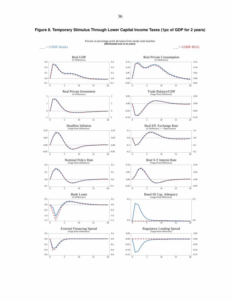
36

Figure 8. Temporary Stimulus Through Lower Capital Income Taxes (1pc of GDP for 2 years)

Percent or percentage point deviation from steady-state baseline(Horizontal axis is in years)

___ = GIMF-Banks _ _ = GIMF-BGG

-0.1

0.0

0.1

0.2

0.3

-0.1

0.0

0.1

0.2

0.3

0 5 10 15 20

Real GDP(% Difference)

-0.05

0.00

0.05

0.10

0.15

-0.05

0.00

0.05

0.10

0.15

0 5 10 15 20

Real Private Consumption(% Difference)

-1

0

1

2

-1

0

1

2

0 5 10 15 20

Real Private Investment(% Difference)

-0.10

-0.05

0.00

0.05

-0.10

-0.05

0.00

0.05

0 5 10 15 20

Trade Balance/GDP(%age Point Difference)

-0.05

0.00

0.05

0.10

-0.05

0.00

0.05

0.10

0 5 10 15 20

Headline Inflation(%age Point Difference)

-0.2

-0.1

0.0

0.1

-0.2

-0.1

0.0

0.1

0 5 10 15 20

Real Eff. Exchange Rate(% Difference; + = Depreciation)

-0.1

0.0

0.1

0.2

-0.1

0.0

0.1

0.2

0 5 10 15 20

Nominal Policy Rate(%age Point Difference)

-0.05

0.00

0.05

0.10

-0.05

0.00

0.05

0.10

0 5 10 15 20

Real S-T Interest Rate(%age Point Difference)

-1.5

-1.0

-0.5

0.0

0.5

-1.5

-1.0

-0.5

0.0

0.5

0 5 10 15 20

Bank Loans(% Difference)

0.0

0.5

0.0

0.5

0 5 10 15 20

Basel III Cap. Adequacy (%age Point Difference)

-0.6

-0.4

-0.2

-0.0

0.2

-0.6

-0.4

-0.2

-0.0

0.2

0 5 10 15 20

External Financing Spread(%age Point Difference)

-0.15

-0.10

-0.05

-0.00

0.05

-0.15

-0.10

-0.05

-0.00

0.05

0 5 10 15 20

Regulatory Lending Spread(%age Point Difference)

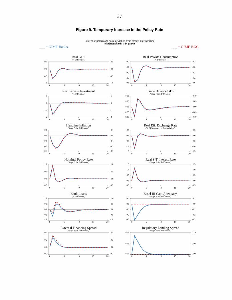
37

Figure 9. Temporary Increase in the Policy Rate

Percent or percentage point deviation from steady-state baseline(Horizontal axis is in years)

___ = GIMF-Banks _ _ = GIMF-BGG

-1.0

-0.5

0.0

0.5

-1.0

-0.5

0.0

0.5

0 5 10 15 20

Real GDP(% Difference)

-0.6

-0.4

-0.2

-0.0

0.2

-0.6

-0.4

-0.2

-0.0

0.2

0 5 10 15 20

Real Private Consumption(% Difference)

-2

-1

0

1

-2

-1

0

1

0 5 10 15 20

Real Private Investment(% Difference)

-0.10

-0.05

0.00

0.05

0.10

-0.10

-0.05

0.00

0.05

0.10

0 5 10 15 20

Trade Balance/GDP(%age Point Difference)

-0.3

-0.2

-0.1

-0.0

0.1

-0.3

-0.2

-0.1

-0.0

0.1

0 5 10 15 20

Headline Inflation(%age Point Difference)

-1.5

-1.0

-0.5

0.0

0.5

-1.5

-1.0

-0.5

0.0

0.5

0 5 10 15 20

Real Eff. Exchange Rate(% Difference; + = Depreciation)

-0.5

0.0

0.5

1.0

-0.5

0.0

0.5

1.0

0 5 10 15 20

Nominal Policy Rate(%age Point Difference)

-0.5

0.0

0.5

1.0

1.5

-0.5

0.0

0.5

1.0

1.5

0 5 10 15 20

Real S-T Interest Rate(%age Point Difference)

-1.0

-0.5

0.0

0.5

1.0

-1.0

-0.5

0.0

0.5

1.0

0 5 10 15 20

Bank Loans(% Difference)

-0.3

-0.2

-0.1

-0.0

0.1

-0.3

-0.2

-0.1

-0.0

0.1

0 5 10 15 20

Basel III Cap. Adequacy (%age Point Difference)

-0.2

0.0

0.2

0.4

-0.2

0.0

0.2

0.4

0 5 10 15 20

External Financing Spread(%age Point Difference)

0.00

0.05

0.10

0.00

0.05

0.10

0 5 10 15 20

Regulatory Lending Spread(%age Point Difference)

38

Figure 10. Temporary Increase in Private Domestic Demand

Percent or percentage point deviation from steady-state baseline(Horizontal axis is in years)

___ = GIMF-Banks _ _ = GIMF-BGG

-0.5

0.0

0.5

1.0

1.5

-0.5

0.0

0.5

1.0

1.5

0 5 10 15 20

Real GDP(% Difference)

-0.5

0.0

0.5

1.0

1.5

-0.5

0.0

0.5

1.0

1.5

0 5 10 15 20

Real Private Consumption(% Difference)

-2

0

2

4

6

-2

0

2

4

6

0 5 10 15 20

Real Private Investment(% Difference)

-0.3

-0.2

-0.1

-0.0

0.1

-0.3

-0.2

-0.1

-0.0

0.1

0 5 10 15 20

Trade Balance/GDP(%age Point Difference)

-0.1

0.0

0.1

0.2

0.3

-0.1

0.0

0.1

0.2

0.3

0 5 10 15 20

Headline Inflation(%age Point Difference)

-0.4

-0.2

0.0

0.2

0.4

-0.4

-0.2

0.0

0.2

0.4

0 5 10 15 20

Real Eff. Exchange Rate(% Difference; + = Depreciation)

-0.2

0.0

0.2

0.4

0.6

-0.2

0.0

0.2

0.4

0.6

0 5 10 15 20

Nominal Policy Rate(%age Point Difference)

-0.1

0.0

0.1

0.2

0.3

-0.1

0.0

0.1

0.2

0.3

0 5 10 15 20

Real S-T Interest Rate(%age Point Difference)

-1.0

-0.5

0.0

0.5

1.0

-1.0

-0.5

0.0

0.5

1.0

0 5 10 15 20

Bank Loans(% Difference)

-0.1

0.0

0.1

0.2

0.3

-0.1

0.0

0.1

0.2

0.3

0 5 10 15 20

Basel III Cap. Adequacy (%age Point Difference)

-0.2

-0.1

0.0

0.1

-0.2

-0.1

0.0

0.1

0 5 10 15 20

External Financing Spread(%age Point Difference)

-0.10

-0.05

0.00

0.05

-0.10

-0.05

0.00

0.05

0 5 10 15 20

Regulatory Lending Spread(%age Point Difference)

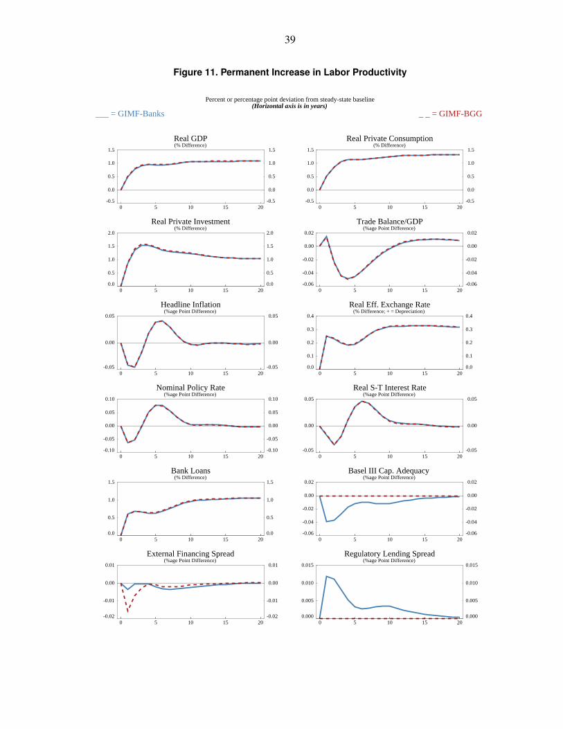
39

Figure 11. Permanent Increase in Labor Productivity

Percent or percentage point deviation from steady-state baseline(Horizontal axis is in years)

___ = GIMF-Banks _ _ = GIMF-BGG

-0.5

0.0

0.5

1.0

1.5

-0.5

0.0

0.5

1.0

1.5

0 5 10 15 20

Real GDP(% Difference)

-0.5

0.0

0.5

1.0

1.5

-0.5

0.0

0.5

1.0

1.5

0 5 10 15 20

Real Private Consumption(% Difference)

0.0

0.5

1.0

1.5

2.0

0.0

0.5

1.0

1.5

2.0

0 5 10 15 20

Real Private Investment(% Difference)

-0.06

-0.04

-0.02

0.00

0.02

-0.06

-0.04

-0.02

0.00

0.02

0 5 10 15 20

Trade Balance/GDP(%age Point Difference)

-0.05

0.00

0.05

-0.05

0.00

0.05

0 5 10 15 20

Headline Inflation(%age Point Difference)

0.0

0.1

0.2

0.3

0.4

0.0

0.1

0.2

0.3

0.4

0 5 10 15 20

Real Eff. Exchange Rate(% Difference; + = Depreciation)

-0.10

-0.05

0.00

0.05

0.10

-0.10

-0.05

0.00

0.05

0.10

0 5 10 15 20

Nominal Policy Rate(%age Point Difference)

-0.05

0.00

0.05

-0.05

0.00

0.05

0 5 10 15 20

Real S-T Interest Rate(%age Point Difference)

0.0

0.5

1.0

1.5

0.0

0.5

1.0

1.5

0 5 10 15 20

Bank Loans(% Difference)

-0.06

-0.04

-0.02

0.00

0.02

-0.06

-0.04

-0.02

0.00

0.02

0 5 10 15 20

Basel III Cap. Adequacy (%age Point Difference)

-0.02

-0.01

0.00

0.01

-0.02

-0.01

0.00

0.01

0 5 10 15 20

External Financing Spread(%age Point Difference)

0.000

0.005

0.010

0.015

0.000

0.005

0.010

0.015

0 5 10 15 20

Regulatory Lending Spread(%age Point Difference)

40

Figure 12. Ten-Year Increase in Labor Productivity Growth

Percent or percentage point deviation from steady-state baseline(Horizontal axis is in years)

___ = GIMF-Banks _ _ = GIMF-BGG

-1

0

1

2

3

-1

0

1

2

3

0 5 10 15 20

Real GDP(% Difference)

-1

0

1

2

3

-1

0

1

2

3

0 5 10 15 20

Real Private Consumption(% Difference)

0

1

2

3

0

1

2

3

0 5 10 15 20

Real Private Investment(% Difference)

-0.3

-0.2

-0.1

-0.0

0.1

-0.3

-0.2

-0.1

-0.0

0.1

0 5 10 15 20

Trade Balance/GDP(%age Point Difference)

-0.1

0.0

0.1

0.2

-0.1

0.0

0.1

0.2

0 5 10 15 20

Headline Inflation(%age Point Difference)

-1.0

-0.5

0.0

0.5

1.0

-1.0

-0.5

0.0

0.5

1.0

0 5 10 15 20

Real Eff. Exchange Rate(% Difference; + = Depreciation)

-0.2

0.0

0.2

0.4

-0.2

0.0

0.2

0.4

0 5 10 15 20

Nominal Policy Rate(%age Point Difference)

-0.1

0.0

0.1

0.2

0.3

-0.1

0.0

0.1

0.2

0.3

0 5 10 15 20

Real S-T Interest Rate(%age Point Difference)

-1

0

1

2

3

-1

0

1

2

3

0 5 10 15 20

Bank Loans(% Difference)

-0.05

0.00

0.05

0.10

-0.05

0.00

0.05

0.10

0 5 10 15 20

Basel III Cap. Adequacy (%age Point Difference)

-0.10

-0.05

0.00

0.05

-0.10

-0.05

0.00

0.05

0 5 10 15 20

External Financing Spread(%age Point Difference)

-0.03

-0.02

-0.01

0.00

0.01

-0.03

-0.02

-0.01

0.00

0.01

0 5 10 15 20

Regulatory Lending Spread(%age Point Difference)

41

Figure 13. Permanent Drop in Wage Markup

Percent or percentage point deviation from steady-state baseline(Horizontal axis is in years)

___ = GIMF-Banks _ _ = GIMF-BGG

-1

0

1

2

-1

0

1

2

0 5 10 15 20

Real GDP(% Difference)

-1

0

1

2

-1

0

1

2

0 5 10 15 20

Real Private Consumption(% Difference)

0

1

2

3

0

1

2

3

0 5 10 15 20

Real Private Investment(% Difference)

0.0

0.1

0.2

0.3

0.0

0.1

0.2

0.3

0 5 10 15 20

Trade Balance/GDP(%age Point Difference)

-0.06

-0.04

-0.02

0.00

0.02

-0.06

-0.04

-0.02

0.00

0.02

0 5 10 15 20

Headline Inflation(%age Point Difference)

0.0

0.5

1.0

1.5

0.0

0.5

1.0

1.5

0 5 10 15 20

Real Eff. Exchange Rate(% Difference; + = Depreciation)

-0.10

-0.05

0.00

0.05

-0.10

-0.05

0.00

0.05

0 5 10 15 20

Nominal Policy Rate(%age Point Difference)

-0.10

-0.05

0.00

0.05

-0.10

-0.05

0.00

0.05

0 5 10 15 20

Real S-T Interest Rate(%age Point Difference)

0.0

0.5

1.0

1.5

2.0

0.0

0.5

1.0

1.5

2.0

0 5 10 15 20

Bank Loans(% Difference)

-0.10

-0.05

0.00

0.05

-0.10

-0.05

0.00

0.05

0 5 10 15 20

Basel III Cap. Adequacy (%age Point Difference)

-0.10

-0.05

0.00

0.05

-0.10

-0.05

0.00

0.05

0 5 10 15 20

External Financing Spread(%age Point Difference)

-0.02

-0.01

0.00

0.01

0.02

-0.02

-0.01

0.00

0.01

0.02

0 5 10 15 20

Regulatory Lending Spread(%age Point Difference)

42

Figure 14. Permanent Drop in Price Markup

Percent or percentage point deviation from steady-state baseline(Horizontal axis is in years)

___ = GIMF-Banks _ _ = GIMF-BGG

-2

0

2

4

6

-2

0

2

4

6

0 5 10 15 20

Real GDP(% Difference)

-2

0

2

4

6

-2

0

2

4

6

0 5 10 15 20

Real Private Consumption(% Difference)

0

5

10

15

0

5

10

15

0 5 10 15 20

Real Private Investment(% Difference)

-0.6

-0.4

-0.2

-0.0

0.2

-0.6

-0.4

-0.2

-0.0

0.2

0 5 10 15 20

Trade Balance/GDP(%age Point Difference)

-0.2

0.0

0.2

0.4

-0.2

0.0

0.2

0.4

0 5 10 15 20

Headline Inflation(%age Point Difference)

0

1

2

3

0

1

2

3

0 5 10 15 20

Real Eff. Exchange Rate(% Difference; + = Depreciation)

-0.5

0.0

0.5

1.0

-0.5

0.0

0.5

1.0

0 5 10 15 20

Nominal Policy Rate(%age Point Difference)

-0.2

0.0

0.2

0.4

0.6

-0.2

0.0

0.2

0.4

0.6

0 5 10 15 20

Real S-T Interest Rate(%age Point Difference)

0

2

4

6

8

0

2

4

6

8

0 5 10 15 20

Bank Loans(% Difference)

-0.2

0.0

0.2

0.4

0.6

-0.2

0.0

0.2

0.4

0.6

0 5 10 15 20

Basel III Cap. Adequacy (%age Point Difference)

-0.6

-0.4

-0.2

-0.0

0.2

-0.6

-0.4

-0.2

-0.0

0.2

0 5 10 15 20

External Financing Spread(%age Point Difference)

-0.15

-0.10

-0.05

-0.00

0.05

-0.15

-0.10

-0.05

-0.00

0.05

0 5 10 15 20

Regulatory Lending Spread(%age Point Difference)

43

Figure 15. Permanent Increase in Tariffs

Percent or percentage point deviation from steady-state baseline(Horizontal axis is in years)

___ = GIMF-Banks _ _ = GIMF-BGG

-1.0

-0.5

0.0

0.5

-1.0

-0.5

0.0

0.5

0 5 10 15 20

Real GDP(% Difference)

-0.5

0.0

0.5

1.0

1.5

-0.5

0.0

0.5

1.0

1.5

0 5 10 15 20

Real Private Consumption(% Difference)

-3

-2

-1

0

1

-3

-2

-1

0

1

0 5 10 15 20

Real Private Investment(% Difference)

-0.4

-0.2

0.0

0.2

-0.4

-0.2

0.0

0.2

0 5 10 15 20

Trade Balance/GDP(%age Point Difference)

-0.1

0.0

0.1

0.2

-0.1

0.0

0.1

0.2

0 5 10 15 20

Headline Inflation(%age Point Difference)

-10

-5

0

5

-10

-5

0

5

0 5 10 15 20

Real Eff. Exchange Rate(% Difference; + = Depreciation)

-0.2

-0.1

0.0

0.1

0.2

-0.2

-0.1

0.0

0.1

0.2

0 5 10 15 20

Nominal Policy Rate(%age Point Difference)

-0.10

-0.05

0.00

0.05

0.10

-0.10

-0.05

0.00

0.05

0.10

0 5 10 15 20

Real S-T Interest Rate(%age Point Difference)

-1.5

-1.0

-0.5

0.0

0.5

-1.5

-1.0

-0.5

0.0

0.5

0 5 10 15 20

Bank Loans(% Difference)

-0.04

-0.02

0.00

0.02

-0.04

-0.02

0.00

0.02

0 5 10 15 20

Basel III Cap. Adequacy (%age Point Difference)

-0.05

0.00

0.05

0.10

0.15

-0.05

0.00

0.05

0.10

0.15

0 5 10 15 20

External Financing Spread(%age Point Difference)

-0.005

0.000

0.005

0.010

-0.005

0.000

0.005

0.010

0 5 10 15 20

Regulatory Lending Spread(%age Point Difference)

44

Figure 16. Temporary Increase in Borrower Riskiness - Equal External Financing Spreads

Percent or percentage point deviation from steady-state baseline(Horizontal axis is in years)

___ = GIMF-Banks _ _ = GIMF-BGG

-0.4

-0.2

0.0

0.2

-0.4

-0.2

0.0

0.2

0 5 10 15 20

Real GDP(% Difference)

-0.2

-0.1

0.0

0.1

-0.2

-0.1

0.0

0.1

0 5 10 15 20

Real Private Consumption(% Difference)

-3

-2

-1

0

1

-3

-2

-1

0

1

0 5 10 15 20

Real Private Investment(% Difference)

-0.05

0.00

0.05

0.10

-0.05

0.00

0.05

0.10

0 5 10 15 20

Trade Balance/GDP(%age Point Difference)

-0.15

-0.10

-0.05

-0.00

0.05

-0.15

-0.10

-0.05

-0.00

0.05

0 5 10 15 20

Headline Inflation(%age Point Difference)

-0.3

-0.2

-0.1

-0.0

0.1

-0.3

-0.2

-0.1

-0.0

0.1

0 5 10 15 20

Real Eff. Exchange Rate(% Difference; + = Depreciation)

-0.3

-0.2

-0.1

-0.0

0.1

-0.3

-0.2

-0.1

-0.0

0.1

0 5 10 15 20

Nominal Policy Rate(%age Point Difference)

-0.15

-0.10

-0.05

-0.00

0.05

-0.15

-0.10

-0.05

-0.00

0.05

0 5 10 15 20

Real S-T Interest Rate(%age Point Difference)

-3

-2

-1

0

1

-3

-2

-1

0

1

0 5 10 15 20

Bank Loans(% Difference)

-3

-2

-1

0

1

-3

-2

-1

0

1

0 5 10 15 20

Basel III Cap. Adequacy (%age Point Difference)

-0.5

0.0

0.5

1.0

1.5

-0.5

0.0

0.5

1.0

1.5

0 5 10 15 20

External Financing Spread(%age Point Difference)

0.0

0.2

0.4

0.6

0.8

0.0

0.2

0.4

0.6

0.8

0 5 10 15 20

Regulatory Lending Spread(%age Point Difference)

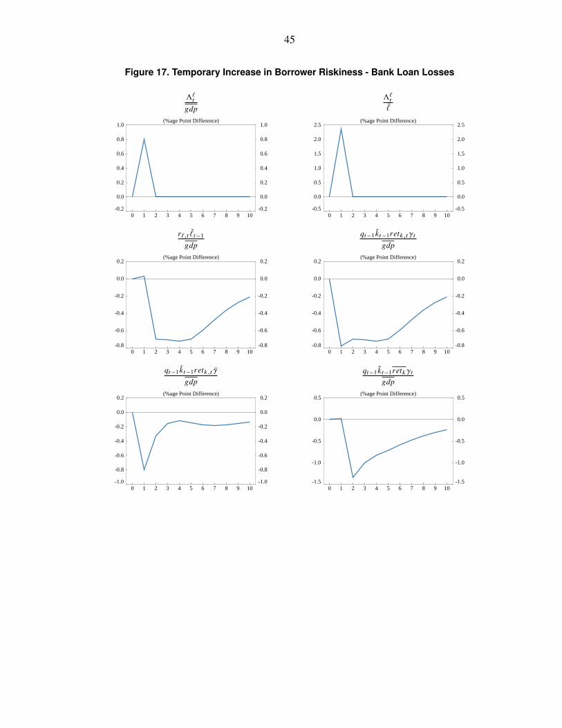
45

Figure 17. Temporary Increase in Borrower Riskiness - Bank Loan Losses

Λ`t

gdpΛ`t¯

-0.2

0.0

0.2

0.4

0.6

0.8

1.0

-0.2

0.0

0.2

0.4

0.6

0.8

1.0

0 1 2 3 4 5 6 7 8 9 10

(%age Point Difference)

-0.5

0.0

0.5

1.0

1.5

2.0

2.5

-0.5

0.0

0.5

1.0

1.5

2.0

2.5

0 1 2 3 4 5 6 7 8 9 10

(%age Point Difference)

r`,t ˇt−1

gdpqt−1 kt−1retk ,tγt

gdp

-0.8

-0.6

-0.4

-0.2

0.0

0.2

-0.8

-0.6

-0.4

-0.2

0.0

0.2

0 1 2 3 4 5 6 7 8 9 10

(%age Point Difference)

-0.8

-0.6

-0.4

-0.2

0.0

0.2

-0.8

-0.6

-0.4

-0.2

0.0

0.2

0 1 2 3 4 5 6 7 8 9 10

(%age Point Difference)

qt−1 kt−1retk ,t γgdp

qt−1 kt−1retkγtgdp

-1.0

-0.8

-0.6

-0.4

-0.2

0.0

0.2

-1.0

-0.8

-0.6

-0.4

-0.2

0.0

0.2

0 1 2 3 4 5 6 7 8 9 10

(%age Point Difference)

-1.5

-1.0

-0.5

0.0

0.5

-1.5

-1.0

-0.5

0.0

0.5

0 1 2 3 4 5 6 7 8 9 10

(%age Point Difference)

46

Figure 18. Temporary Increase in Borrower Riskiness - Equal Shock Sizes

Percent or percentage point deviation from steady-state baseline(Horizontal axis is in years)

___ = GIMF-Banks _ _ = GIMF-BGG

-0.3

-0.2

-0.1

-0.0

0.1

-0.3

-0.2

-0.1

-0.0

0.1

0 5 10 15 20

Real GDP(% Difference)

-0.15

-0.10

-0.05

-0.00

0.05

-0.15

-0.10

-0.05

-0.00

0.05

0 5 10 15 20

Real Private Consumption(% Difference)

-2

-1

0

1

-2

-1

0

1

0 5 10 15 20

Real Private Investment(% Difference)

-0.05

0.00

0.05

0.10

-0.05

0.00

0.05

0.10

0 5 10 15 20

Trade Balance/GDP(%age Point Difference)

-0.10

-0.05

0.00

0.05

-0.10

-0.05

0.00

0.05

0 5 10 15 20

Headline Inflation(%age Point Difference)

-0.15

-0.10

-0.05

-0.00

0.05

-0.15

-0.10

-0.05

-0.00

0.05

0 5 10 15 20

Real Eff. Exchange Rate(% Difference; + = Depreciation)

-0.2

-0.1

0.0

0.1

-0.2

-0.1

0.0

0.1

0 5 10 15 20

Nominal Policy Rate(%age Point Difference)

-0.10

-0.05

0.00

0.05

-0.10

-0.05

0.00

0.05

0 5 10 15 20

Real S-T Interest Rate(%age Point Difference)

-2

-1

0

1

-2

-1

0

1

0 5 10 15 20

Bank Loans(% Difference)

-1.5

-1.0

-0.5

0.0

0.5

-1.5

-1.0

-0.5

0.0

0.5

0 5 10 15 20

Basel III Cap. Adequacy (%age Point Difference)

-0.5

0.0

0.5

1.0

1.5

-0.5

0.0

0.5

1.0

1.5

0 5 10 15 20

External Financing Spread(%age Point Difference)

0.0

0.5

0.0

0.5

0 5 10 15 20

Regulatory Lending Spread(%age Point Difference)

47

Figure 19. Fixed versus Countercyclical MCAR

Percent or percentage point deviation from steady-state baseline(Horizontal axis is in years)

___ = Fixed MCAR _ _ = Countercyclical MCAR

-0.4

-0.3

-0.2

-0.1

0.0

-0.4

-0.3

-0.2

-0.1

0.0

0 5 10 15 20

Real GDP(% Difference)

-0.20

-0.15

-0.10

-0.05

0.00

-0.20

-0.15

-0.10

-0.05

0.00

0 5 10 15 20

Real Private Consumption(% Difference)

-3

-2

-1

0

1

-3

-2

-1

0

1

0 5 10 15 20

Real Private Investment(% Difference)

-0.05

0.00

0.05

0.10

-0.05

0.00

0.05

0.10

0 5 10 15 20

Trade Balance/GDP(%age Point Difference)

-0.15

-0.10

-0.05

-0.00

0.05

-0.15

-0.10

-0.05

-0.00

0.05

0 5 10 15 20

Headline Inflation(%age Point Difference)

-0.3

-0.2

-0.1

-0.0

0.1

-0.3

-0.2

-0.1

-0.0

0.1

0 5 10 15 20

Real Eff. Exchange Rate(% Difference; + = Depreciation)

-0.3

-0.2

-0.1

-0.0

0.1

-0.3

-0.2

-0.1

-0.0

0.1

0 5 10 15 20

Nominal Policy Rate(%age Point Difference)

-0.15

-0.10

-0.05

-0.00

0.05

-0.15

-0.10

-0.05

-0.00

0.05

0 5 10 15 20

Real S-T Interest Rate(%age Point Difference)

-3

-2

-1

0

1

-3

-2

-1

0

1

0 5 10 15 20

Bank Loans(% Difference)

-3

-2

-1

0

1

-3

-2

-1

0

1

0 5 10 15 20

Basel III Cap. Adequacy (%age Point Difference)

-0.5

0.0

0.5

1.0

1.5

-0.5

0.0

0.5

1.0

1.5

0 5 10 15 20

External Financing Spread(%age Point Difference)

0.0

0.2

0.4

0.6

0.8

0.0

0.2

0.4

0.6

0.8

0 5 10 15 20

Regulatory Lending Spread(%age Point Difference)

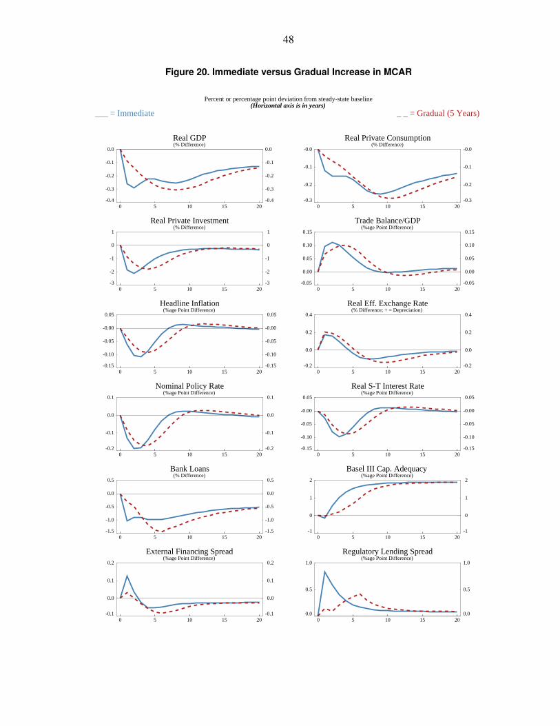
48

Figure 20. Immediate versus Gradual Increase in MCAR

Percent or percentage point deviation from steady-state baseline(Horizontal axis is in years)

___ = Immediate _ _ = Gradual (5 Years)

-0.4

-0.3

-0.2

-0.1

0.0

-0.4

-0.3

-0.2

-0.1

0.0

0 5 10 15 20

Real GDP(% Difference)

-0.3

-0.2

-0.1

-0.0

-0.3

-0.2

-0.1

-0.0

0 5 10 15 20

Real Private Consumption(% Difference)

-3

-2

-1

0

1

-3

-2

-1

0

1

0 5 10 15 20

Real Private Investment(% Difference)

-0.05

0.00

0.05

0.10

0.15

-0.05

0.00

0.05

0.10

0.15

0 5 10 15 20

Trade Balance/GDP(%age Point Difference)

-0.15

-0.10

-0.05

-0.00

0.05

-0.15

-0.10

-0.05

-0.00

0.05

0 5 10 15 20

Headline Inflation(%age Point Difference)

-0.2

0.0

0.2

0.4

-0.2

0.0

0.2

0.4

0 5 10 15 20

Real Eff. Exchange Rate(% Difference; + = Depreciation)

-0.2

-0.1

0.0

0.1

-0.2

-0.1

0.0

0.1

0 5 10 15 20

Nominal Policy Rate(%age Point Difference)

-0.15

-0.10

-0.05

-0.00

0.05

-0.15

-0.10

-0.05

-0.00

0.05

0 5 10 15 20

Real S-T Interest Rate(%age Point Difference)

-1.5

-1.0

-0.5

0.0

0.5

-1.5

-1.0

-0.5

0.0

0.5

0 5 10 15 20

Bank Loans(% Difference)

-1

0

1

2

-1

0

1

2

0 5 10 15 20

Basel III Cap. Adequacy (%age Point Difference)

-0.1

0.0

0.1

0.2

-0.1

0.0

0.1

0.2

0 5 10 15 20

External Financing Spread(%age Point Difference)

0.0

0.5

1.0

0.0

0.5

1.0

0 5 10 15 20

Regulatory Lending Spread(%age Point Difference)