School of Economics and Management

Department of Business Administration

FEKN90

Business Administration-

Degree Project Master of Science in Business and Economics

Spring term of 2013

Bankruptcy Prediction with Financial

Ratios

- Examining Differences across Industries and Time

Author:

David Lundqvist

Jakob Strand

Supervisor:

Jens Forssbaeck

1

Abstract

Title: Bankruptcy Prediction with Financial Ratios – Examining

Differences across Industries and Time.

Date of Seminar: May 31, 2013

Course: FEKN90: Master thesis in Business Administration, 30

University Credit Points (30 ECTS)

Authors: David Lundqvist and Jakob Strand

Advisor: Jens Forssbaeck

Five key words: Credit Risk, Bankruptcy Prediction Modeling, Logit

Regression, Financial Ratios, Industry Differences

Purpose: The purpose of this study is to examine how well different

financial ratios can predict bankruptcy across industries

and time. The study also examine whether including

industry differences in a prediction model can increase its

accuracy.

Methodology: Bankruptcy prediction models were estimated using

logistic regression for each year between 2006 and 2011,

with and without interaction terms accounting for industry

effects. These were analyzed and tested on a holdout

sample for their classification abilities.

Theoretical perspectives: This study is influenced by previous research within

bankruptcy prediction modeling performed by for example

Ohlson (1980).

Empirical foundation: 311,930 annual reports from non-bankrupt companies and

5,257 annual reports from bankrupt companies were

analyzed, covering the time period 2006 to 2011.

Conclusions: The study shows that the bankruptcy-prediction ability of

different financial ratios varies between years. However,

only in some cases, significant differences between

industries were found. The overall classification ability

was not significantly increased when including the

industry effects but using some specified cut-off values, a

marginal increase was found.

2

Acknowledgement

The working process of this study has been rewarding in many ways and we have

broadened our knowledge of statistical methodology and credit risk modeling.

We would like to thank all of those who made this master thesis possible. First of all,

we would like to thank our supervisor Jens Forssbaeck who has helped us throughout

this thesis with advice and support.

Furthermore, we would like to thank Tomas Gustafsson, Lena Kulling, Torbjörn

Johansson, Jens Skaring, Johan Lofall and Nina Larsson at Swedbank. Their input gave

us new perspectives and information which has helped us throughout the process.

3

Contents Abstract ............................................................................................................................. 1

Acknowledgement ............................................................................................................ 2

1 INTRODUCTION ......................................................................................................... 5

1.1 Background ............................................................................................................. 5

1.2 Problem Discussion ................................................................................................ 7

1.3 Research Questions ................................................................................................. 8

1.4 Purpose .................................................................................................................... 9

1.5 Delimitations ........................................................................................................... 9

1.6 Thesis Outline ......................................................................................................... 9

2 THEORETICAL FRAMEWORK ............................................................................... 10

2.1 Corporate Default and Failure .............................................................................. 10

2.2 Bankruptcy Regulations ........................................................................................ 11

2.3 Credit Risk Models ............................................................................................... 11

2.3.1 Accounting-Based Models ............................................................................. 12

2.3.2 Market-Based Models .................................................................................... 14

2.3.3 Hazard Models ............................................................................................... 16

2.4 Previous Research around Industry Characteristics .............................................. 16

2.5 Evaluation of Prediction Accuracy in the Literature ............................................ 19

2.6 Discussion on Motives for Using Empirical Models ............................................ 20

2.7 Hypothesis ............................................................................................................ 20

3 METHODOLOGY ...................................................................................................... 22

3.1 Choice of Statistical Model ................................................................................... 22

3.2 Data Collection ..................................................................................................... 24

3.2.1 Data Sample ................................................................................................... 24

3.2.2 Original Sample of Financial Ratios .............................................................. 27

3.3 Data Analysis ........................................................................................................ 27

3.3.1 Basic Analysis of the Data and Choice of Industries ..................................... 28

3.3.2 Univariate Analysis and Analysis of Correlations ......................................... 29

3.3.3 The Final Modeling ....................................................................................... 30

3.4 Finding the Optimal Cut-Off Values .................................................................... 30

3.5 Evaluating the Classifying Abilities of the Models .............................................. 32

3.6 Methodological Discussion................................................................................... 33

4

4 EMPIRICAL RESULTS.............................................................................................. 36

4.1 Presentation of Descriptive Statistics ................................................................... 36

4.2 Results from Analysis of Ratios ........................................................................... 36

4.2.1 Univariate Analysis ........................................................................................ 36

4.2.2 Industry Differences ...................................................................................... 37

4.2.3 Correlations .................................................................................................... 38

4.3 Models without Industry Effects ........................................................................... 39

4.4 Models with Industry Effects ................................................................................ 41

4.5 Results from ROC Analysis .................................................................................. 43

4.6 Prediction Accuracy .............................................................................................. 44

5 DISCUSSION .............................................................................................................. 46

6 CONCLUSION ............................................................................................................ 49

6.1 Conclusions ........................................................................................................... 49

6.2 Suggestions for Further Research ......................................................................... 50

REFERENCES ............................................................................................................... 52

Articles ........................................................................................................................ 52

Books .......................................................................................................................... 54

Internet Sources .......................................................................................................... 55

Exhibit 1 – List of Financial Ratios ................................................................................ 57

Exhibit 2 – Bankruptcies across Industries ..................................................................... 58

Exhibit 3 – Univariate Analysis ...................................................................................... 59

Exhibit 4 – Financial Ratios across Industries ................................................................ 60

Exhibit 5 – Correlations among Financial Ratios ........................................................... 61

Exhibit 6 – Prediction Models excluding Industry Effects ............................................. 62

Exhibit 7 – Prediction Models including Industry Effects ............................................. 64

Exhibit 8 – Total Marginal Effects for Each Industry .................................................... 67

Exhibit 9 – ROC Results ................................................................................................. 70

Exhibit 10 – Prediction Accuracy ................................................................................... 74

5

1 INTRODUCTION

This chapter starts with a short background to the subject. Next a problem discussion

follows that lead up to the research questions, purpose and delimitations of the study.

The chapter ends with a short presentation of the thesis outline.

1.1 Background

Every year, thousands of companies find themselves in financial difficulties which in

many cases lead to bankruptcy. Over the last decade the number of bankruptcies in

Sweden has followed a cyclical pattern. After the IT bubble burst in the beginning of the

millennia the number was on top but then steadily decreased until the new crisis hit the

world economy in 2008. In 2009 the number of bankruptcies in Sweden peaked at 6,428

bankruptcies and has since then decreased to a number of 6,163 in 2012. Figure 1.1

illustrates how the bankruptcies have evolved over time (The Swedish Agency for

Growth Policy Analysis, 2013).

Figure 1.1

Number of corporate bankruptcies per year in Sweden between 2001 and 2012

This development has also been observed among people working with bankruptcies.

Lena Kulling, functional manager at the Collections department at Swedbank, describes

a similar pattern. According to her, they experienced a peak of bankruptcies among their

borrowers in 2008 thereafter followed by a decline (personal communication, 2013-02-

25).

6

The development of bankruptcies has not looked the same across industries. Figure 1.2

below illustrates how the number of bankruptcies for four different industries has

developed over the last decade (The Swedish Agency for Growth Policy Analysis,

2013).

Figure 1.2

Number of bankruptcies per year in Sweden within four industries

Clearly, there are differences across industries. These differences also affect the

investors and their willingness to invest money in the industries. According to Torbjörn

Johansson, a credit specialist with experience of credit granting at Swedbank, they can

be very skeptical granting loans to some industries such as the newly deregulated and

highly competitive pharmaceutical industry (personal communication, 2013-02-25).

There are many theories and arguments for why companies go bankrupt. Schumpeter

(1942) called it “creative destruction”, a process of industrial mutation where new

economic structures are destroying old ones. According to this philosophy, bankruptcies

are a natural part of the capitalism and make it possible for new companies and

industries to grow. Bankruptcies are a major phenomenon in the economy and many

would probably admit that they can be problematic. Not only a firm’s investors are

affected by a bankruptcy but also other stakeholders. For example, in 2012, 25,466

employees in Sweden were affected by the bankruptcy of their employer (The Swedish

Agency for Growth Policy Analysis, 2013).

7

Whether or not bankruptcies are seen as problematic, it is valuable for stakeholders to

know the risk of a corporate bankruptcy. Investors may want to incorporate the risk into

the required rate of return and employees may want to start looking for another job. A

firm’s suppliers may want to know the risk before granting trade credits. For these and

many other stakeholders, a lot of tools for risk evaluations exist.

1.2 Problem Discussion

The situations are many in which credit risk evaluations are necessary. Stakeholders in

need for such evaluations have two options. Either they can rely on existing credit

ratings offered by credit rating agencies such as Moody’s, or they can make their own

evaluations.

Credit rating agencies have been criticized on a number of areas. First of all, their

competence has been questioned after a number of misjudgments or failures such as not

being able to detect the true financial condition of Enron (Frost, 2007). There have also

been questions whether rating agencies can manage the conflict of interest of having an

economic interests in basing a credit rating on anything else than creditworthiness

(Frost, 2007). However, such a problem has been tested for without any evidence of its

existence (Covitz & Harrison, 2003).

If one decides to make their own credit risk evaluation he or she has different available

models to utilize. One type of credit risk models are the market-based models. These

models employ option-pricing theory to make estimates of corporate default (Charitou

et al., 2008). A problem with these models is that they cannot be applied directly on

privately held companies since they depend on market values and the volatility in

market value returns.

Another option is to use an evaluation model based on accounting data. Over the last 50

years a lot of empirical studies have been made within this field of bankruptcy

prediction modeling.

Altman (1968) was the first one to use multivariate statistical modeling in his “Z-score

model” to find combinations of financial ratios that can indicate bankruptcy risk. The

ratios included in Altman’s model were for example a return on assets ratio and a

leverage ratio. Another model was estimated by Ohlson in 1980. He utilized a method

not previously used in the bankruptcy prediction research called logistic regression and

8

modeled different financial ratios such as liquidity and leverage. After him, a lot of

researchers have performed similar studies. However, many of the existing models are

very general and are estimated from a sample of companies from different industries

without much consideration to how these industry differences may affect the results.

One reason why general models may be less accurate compared to industry-adapted

models can be understood by examining the average financial ratios among different

industries. For example, the sales-to-assets ratio is on average 1.72 for wholesale and

retail firms in the US but 0.54 for manufacturing firms (Brandow Company, 2013). This

ratio was included in Altman’s (1968) original Z-score model with a positive

coefficient, indicating that a higher value leads to a higher Z-score and a lower risk of

bankruptcy. Applying Altman’s model on these two industries would therefore (all other

variables being equal) yield lower Z-scores for the manufacturing industry, even though

the bankruptcy risk may not be higher in this industry. It is reasonable to think that there

is a structural difference between these two industries that can explain at least parts of

this difference in averages. A manufacturing company probably needs much more

machines and other assets to be able to produce and sell their goods, while a retail

company only distributes goods and does not produce much on their own. By

understanding these differences in ratios between industries, better bankruptcy risk

estimation can hopefully be made.

Another problem is related to the time dimension. Altman (1968) used a data sample

covering 20 years, and Ohlson’s (1980) sample covered 7 years. Pooling financial data

from many years in this way will lead to that both historical and recent financial data

will be considered of equal weight and that the time dimension is lost. By analyzing

differences in financial ratios and their predictive ability across years, the severity of

pooling data can be further understood.

1.3 Research Questions

How does the bankruptcy-prediction ability for a set of common financial ratios

vary across a number of industries and across time?

Do incorporating industry-variations change the performance of a bankruptcy-

prediction model compared to a model without these variations?

9

1.4 Purpose

The main purpose of this thesis is to study how financial ratios can have different

bankruptcy-indicating abilities across industries and time. The goal is to estimate

models in a similar way as Ohlson (1980) did, and then add industry-depending

interaction terms and dummies to count for the differences between industries. The final

purpose is to compare the prediction accuracy of the estimated models to see what effect

the industry-adaptation can have on the results. The results from this study can

hopefully increase the understanding among business researchers and academics on how

financial ratios vary as bankruptcy indicators across industries and time, and inspire

researchers for further research. Hopefully the results can also serve as a new tool for

some market participants in need for a better way to predict corporate bankruptcy.

1.5 Delimitations

This study will only focus on how an empirically estimated model for bankruptcy

prediction based on logistic regression can be adapted to and explain industry

differences. Alternative models or estimation techniques will not be examined. The

companies studied are privately held Swedish companies. Sweden was chosen as the

target because of the rich amount of financial data available through the Swedish

Companies Registration Office. To be able to model industry characteristics, only five

industries were chosen for this further analysis. These five industries are presented in

section 3.3.1. The study can hopefully increase the understanding on how different

financial ratios can indicate bankruptcy across the five chosen industries and how they

vary over time. The study will not be able to answer questions regarding how other

factors such as “soft variables” or macroeconomic conditions can explain bankruptcies.

1.6 Thesis Outline

The upcoming chapter will introduce the reader to fundamental concepts and models

within the bankruptcy literature. Previous studies concerning industry differences and

the attempts to incorporate these into prediction models will also be discussed. Chapter

3 describes the methodology used in this study. Step by step the process that lead up to

the results is described. The results of the study will be presented in chapter 4, analyzed

in chapter 5, and finally concluded in chapter 6.

10

2 THEORETICAL FRAMEWORK

This chapter starts with a discussion on terminology and a brief review of bankruptcy

legislation. Next, a number of accounting-based, market-based and hazard models will

be reviewed to outline their fundamental differences, followed by a review of some

studies on industry-differences. In the end, a hypothesis for the study is presented.

2.1 Corporate Default and Failure

Default is a common word in the literature, often associated with the potential negative

event in a situation where credit risk is present. According to the Dictionary of Finance

and Banking (Oxford Reference, 2012), default can be defined as the failure to make

required payments.

Default does not automatically lead to bankruptcy though. Many companies fail to make

required payments on loans because of temporary illiquidity, and these companies can

often negotiate with the bank to find another solution than to go bankrupt. According to

Jens Skaring, head of the Financial Restructuring and Recovery department at

Swedbank, they can for example postpone the reinstallments or renegotiate the interest

rate (personal communication, 2013-03-06).

Failure is another common word, particularly within accounting-based modeling

literature. Beaver (1966) defined failure as the inability of a firm to pay its financial

obligations as they mature – a definition similar to the definition of default presented

above. Altman (1968) and Ohlson (1980) on the other hand used the term failure in a

legal perspective on companies that have filed for bankruptcy. Skogsvik (1990) finally,

associated failure not only with legal bankruptcy but also with composition agreements,

voluntary shut-downs of primary production activities and receipt of substantial

subsidies from the state.

Clearly, there are many terms and definitions being used. Since the definition of failure

is often the basis for the selection of companies to study in the bankruptcy research, the

definition used affects the results and the conclusions that can be made.

The definition of failure used in this study is similar to the definition used by Altman

(1968) and Ohlson (1980). Companies that have failed are companies that have filed for

bankruptcy and begun or ended their bankruptcy process. Companies that have been

11

voluntary shut down are not considered failed companies since no information are held

on what cause is behind the shut-down.

2.2 Bankruptcy Regulations

In order to understand which firms can be classified as bankrupt and what conditions

that can start this process, it is a good idea to study the bankruptcy regulations. Since

this study is performed on Swedish companies, the Swedish regulatory framework will

be examined. A company experiencing liquidity issues can either apply for

reconstruction or bankruptcy. In the case of bankruptcy the creditors will forcefully

claim the assets of the bankrupt company as payment on the outstanding debt. A debtor

can by himself and by the request of a creditor be put into bankruptcy1. A creditor can

file for the bankruptcy of a company if the debtor is insolvent. If nothing else is said, a

debtor is insolvent if the debtor 6 months prior to the filing have not been able to meet

their financial obligations or has been urged by the creditor to pay its debt but neglected

to do so for one week2. However, the creditor is unable to file for bankruptcy of the

debtor if collateral is held, if a third party secures the debt on behalf of the creditor, or

the debt have not yet defaulted and a third party insures its payment3.

When the bankruptcy request is accepted by the district court an independent

administrator that holds the appropriate expertise and experience is selected by the court

to oversee the bankruptcy. Depending on the company one or more administrators can

be appointed4. According to Tomas Gustafsson, manager at the Collections department

at Swedbank, a bankruptcy process takes on average 1.5-2 years but depending on the

size of the company a bankruptcy process can stretch out for much longer periods.

Bankruptcy filings are not the first course of action when a company meets liquidity

problems. Rather than liquidation, the possibility of a restructuration is examined and is

a preferred alternative in many cases (personal communication, 2013-02-25).

2.3 Credit Risk Models

There are two major groups of models for evaluating corporate credit risk. The first

group consists of accounting-based models. These models can be used to predict

corporate failure and are empirically estimated from a sample of failed and non-failed

1 Konkurslag (1987:672), 1 §, 2 §

2 Konkurslag (1987:672), Kap 2. 7-9 §

3 Konkurslag (1987:672), Kap 2. 10 §

4 Konkurslag (1987:672), Kap 7. 1-2 §

12

companies. The other group consists of market-based models. These models on the

other hand rely on a theoretical foundation and use option-pricing theory to value

corporate liabilities and measure the probability of default. This section reviews the

different kinds of models and their characteristics.

2.3.1 Accounting-Based Models

The accounting-based models use information from financial statements, normally in

the form of ratios, to describe the risk of failure of a company. One of the first

researchers to explore the predictive ability of financial ratios was Beaver (1966). He

did a univariate analysis and examined a sample of 79 failed companies, including both

bankrupt companies and companies with other financial problems. He found that cash

flow/total debt and net income/total assets were the two best predictors of failure.

The first multivariate model for bankruptcy classification was presented by Altman

(1968). This model, called Altman’s Z-score model, was based on a statistical method

called multiple discriminant analysis (MDA). Altman used a sample of 66 companies,

of which 33 were companies that had filed for bankruptcy. For each company, he

calculated their values on five different financial ratios. Based on this data, a model was

estimated that was able to classify a company as either a non-bankrupt company or a

company that would go bankrupt within 1-2 years. More specifically, this classification

was made by calculating a Z-score and then comparing it to a cut-off value. Companies

with a higher Z-score than the cut-off value was classified as non-bankrupt while

companies with lower Z-scores were classified as bankrupt. The five financial ratios

that were included in the function are presented in table 2.1 below.

13

Table 2.1

Altman’s Z-Score Model Ohlson’s Model

Variable Definition Variable Definition

X1

(Current assets – current

liabilities)/total assets SIZE

Ln(total assets/GNP price-level

index)

X2

Retained earnings/total

assets TLTA Total liabilities/total assets

X3 EBIT/average total assets WCTA Working capital/total assets

X4

MV of equity/BV of

liabilities CLCA Current liabilities/current assets

X5 Sales/average total assets OENEG 1 if total liabilities exceeds total

assets, 0 otherwise

NITA Net income/total assets

FUTL Funds from operations/total

liabilities

INTWO 1 if net income was negative for

the last two years, 0 otherwise

CHIN Change in net income

The table shows the variables that were included in Altmans (1968) and Ohlson’s (1980) model

After Altman, a lot of other researchers have performed similar studies. Deakin (1972)

concluded that the predictive ability of Altman’s model declined as the number of years

prior bankruptcy increased and estimated models for each of the last five years prior

company bankruptcy. Taffler (1982) on the other hand estimated a model for

bankruptcies in the UK.

Ohlson (1980) criticized Altman and other previous researchers using MDA for

predicting bankruptcy. Using MDA imposes a lot of statistical assumptions that are hard

to meet up to. For example, one assumption is that all independent variables are

normally distributed. Ohlson also presented his own prediction models by instead using

the statistical method called logistic regression. This method avoids the problems of

MDA because it is not based on as strict assumptions (Ohlson, 1980). Nine financial

variables were used in the models and these are presented in table 2.1 above. The table

shows that Ohlson’s model contained variables similar to those Altman used. For

example, both models contained a return on assets ratio, a leverage ratio and a working

capital ratio. However, Ohlson also included two dummy variables. The first dummy

accounted for companies with negative equity capital. According to Ohlson, companies

with a negative equity has a considerably higher probability of going bankrupt and it

14

therefore makes sense to include a variable that accounts for this effect. He also

included a dummy variable that was set to one for companies that had had a negative net

income for the last two years. A problem with the model though is that not all variables

were statistically significant. For example the dummy variable that accounted for

companies with a negative net income for two years in a row was not significant in one

version of the model.

One problem with many accounting-based models, including Altman’s Z-score model

and Ohlson’s model is that they are based on pooled data from many years. Altman’s

model was estimated using financial data from 20 years, and Ohlson’s model used data

from seven years. When pooling data the assumption is made that bankruptcy

predictability of different combinations of ratios is stationary and does not vary over

different economic conditions, and this may not be the case (Mensah, 1984).

2.3.2 Market-Based Models

The market-based models are the other category of credit risk models. What

characterizes these models is that they are based on a theoretical foundation of option

pricing theory. The Merton model, developed by Merton (1974), is considered the first

developed model within this area. His model in turn was based on Black & Scholes

(1973) previous work.

In the Merton model, the equity of a company is viewed as a call option on the

company’s assets (Merton, 1974). The debt of the company is assumed to be a zero-

coupon bond with the face value B, maturing at time τ. In the event that the firm value,

V is higher than B at the maturity date the debt holders get paid the full face value B and

the remaining Vt-B is the equity value that belongs to the shareholders. If Vt<B the firm

goes bankrupt and the bondholders receives the liquidation value while the shareholders

receives nothing. The principal of the debt B is therefore the default barrier which in

option terms can be viewed as the strike price and V can be viewed as the price of the

underlying asset. Based on this reasoning, the call option pricing formula can be used:

( ) ( ) (1)

15

Where

( ) (

)

√ √

(2)

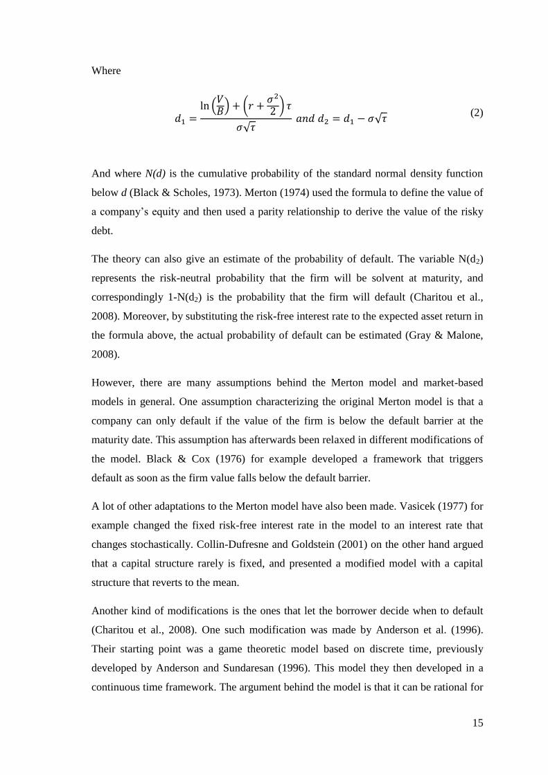
And where N(d) is the cumulative probability of the standard normal density function

below d (Black & Scholes, 1973). Merton (1974) used the formula to define the value of

a company’s equity and then used a parity relationship to derive the value of the risky

debt.

The theory can also give an estimate of the probability of default. The variable N(d2)

represents the risk-neutral probability that the firm will be solvent at maturity, and

correspondingly 1-N(d2) is the probability that the firm will default (Charitou et al.,

2008). Moreover, by substituting the risk-free interest rate to the expected asset return in

the formula above, the actual probability of default can be estimated (Gray & Malone,

2008).

However, there are many assumptions behind the Merton model and market-based

models in general. One assumption characterizing the original Merton model is that a

company can only default if the value of the firm is below the default barrier at the

maturity date. This assumption has afterwards been relaxed in different modifications of

the model. Black & Cox (1976) for example developed a framework that triggers

default as soon as the firm value falls below the default barrier.

A lot of other adaptations to the Merton model have also been made. Vasicek (1977) for

example changed the fixed risk-free interest rate in the model to an interest rate that

changes stochastically. Collin-Dufresne and Goldstein (2001) on the other hand argued

that a capital structure rarely is fixed, and presented a modified model with a capital

structure that reverts to the mean.

Another kind of modifications is the ones that let the borrower decide when to default

(Charitou et al., 2008). One such modification was made by Anderson et al. (1996).

Their starting point was a game theoretic model based on discrete time, previously

developed by Anderson and Sundaresan (1996). This model they then developed in a

continuous time framework. The argument behind the model is that it can be rational for

16

a firm to default on a loan. The reason is that bankruptcy is a costly process and that it

therefore can be rational for the creditor to accept the default and renegotiate the terms

rather than liquidating the company.

2.3.3 Hazard Models

In 2001, Shumway published an article where he criticized the traditional accounting-

based models for being static. He argued that since they only use observations of

companies from a single point in time a lot of information is left out, such as the

company’s development over time. Also, often such single-point observations from

different companies are pooled over many years.

Shumway’s solution was a new technique based on a hazard model. This model is a

kind of survival model where the dependent variable is the time the firm will stay non-

bankrupt. Shumway used corporate data from 30 years and estimated a model where

this “health” was a function of firm age and a combination of different market-based

and accounting-based variables. He concluded that combining market-based and

accounting-based variables increases the accuracy in out-of-sample forecasts.

2.4 Previous Research around Industry Characteristics

Over the years, updated versions of Altman’s Z-score model have been published. One

version is the Z’-score model that is adapted to privately held firms (Altman, 2000).

This model differs in that the market value of equity/book value of debt ratio is

substituted to a similar ratio but with only book values. However, a drawback of the

model is that the model still is estimated using only financial data from publicly held

companies. Another version Altman (2002) presents is the Z’’-score model, which is

adapted to non-manufacturing firms and firms in emerging markets. This model

excludes the ratio sales/total assets because it is a very industry-sensitive ratio according

to Altman.

Other researchers have presented bankruptcy prediction models adapted to other

industries such as the construction industry (Ng et al., 2011), the hospital industry (Al-

Sulaiti & Almwajeh, 2007) and the hotel industry (Kim, 2008). Kim & Gu (2006)

studied the restaurant industry in the US and modeled bankruptcy risk using both MDA

and logistic regression. The two models contain only two independent financial ratios:

total liabilities/total assets, and EBIT/total liabilities. Their study is interesting for two

reasons. First, the study showed that the two methods performed equally well. Second,

17

the models had a high out-of-sample prediction accuracy with 93% of all companies

correctly classified, despite using only two financial ratios.

One problem with the industry-specific models is that they do not tell anything about

differences regarding how the bankruptcy-indicating explanatory power for different

financial ratios varies across industries. Even though a comparison can be made

between different industry-specific models in the literature, such a comparison would

not be very reliable because of differences in financial ratios used and different time

periods for the model estimations.

Dakovic et al. (2010) did a study on Norwegian companies and compared different

methods to build bankruptcy prediction models. One of their models accounts for

industry differences in the intercept by including industry-specific dummy variables.

However, their purpose is to see if one can enhance the bankruptcy prediction accuracy

by examining the best functional form of different financial ratios and less attention is

paid to industrial differences. Since they do not present any numbers on the estimated

coefficients it is not possible draw any conclusions on industry differences in their

results. Also, since no interaction terms are used to account for differences in the

marginal effects of ratios across industries, it would not be possible to draw any

conclusions about these differences either.

Platt and Platt (1990) examined the effects of industry-relative ratios on bankruptcy.

They used seven financial and operational variables and estimated two models. The first

model included the seven ratios and the second model included the same ratios but

industry-normalized by divided by the industry average. Industry effects were also

incorporated through an industry-wide factor in the second model: Two of the variables

included in the model were the product of two other factors. The first of these factors

was the percentage change in total output for the industry the company belonged to. The

second factor was a cash flow ratio and a leverage ratio respectively. The authors found

that the model including industry-relative ratios correctly classified a higher percentage

of the sample. They also found that industry effects were significant on corporate failure

and that the model including the change in industry-output significantly performed

better than the one without this variable.

Chava and Jarrow (2004) take the industry effects analysis one step further. They

analyzed industry effects for four selected industries by using interaction terms in a

18

hazard model, presented in table 2.2 below. The four industry categories included in the

analysis were the finance, insurance, and real estate industry; the transportation,

communications and utilities industry; the manufacturing and minerals industry; and a

miscellaneous grouping of the rest of the industries. The authors conclude that it is

important to include industry effects in a hazard model since the intercept and slope

coefficients are significantly affected by the industry groupings.

They also conclude that the

industry effects significantly

improve the accuracy of the

model. However, a problem

with their model is that they

use very broad industry

groupings and that the fourth

industry is a group of many

different industries. Since the

miscellaneous grouping is

used as the reference industry

and is not assigned any

dummy variable, the other

industries are compared to

this industry. This makes it

hard to interpret the results,

since this group consists of many different industries. Another weakness of their model

is that it only includes two financial ratios – net income over total assets and total

liabilities over total assets. Even though two ratios may be enough to create a good

model, it means that the study does not tell anything about how other ratios may differ

across industries. A third weakness of their study is that they use data from the time

1962 to 1999, which is a very long time period. Over this time period a lot of things

have changed and industries have developed which makes it hard to draw conclusions

of industry differences in today’s world.

The previous studies show that it may be advantageous to adjust a bankruptcy

prediction model to industry differences. However, the only study trying to explain how

bankruptcy-indicating abilities of financial variables may vary across industries is the

Coefficient Variable Explanation

-5.9090*** Intercept

-1.0466*** NITA Net income/total assets

2.2036*** TLTA Total liabilities/total assets

-0.9619*** IND2 Manufacturing & Minerals

-0.7524* IND3 Transport & Utilities

-0.8315** IND4 Finance & Real Estate

-0.2354 NITA*IND2

0.8275*** TLTA*IND2

-1.4547*** NITA*IND3

0.1174 TLTA*IND3

-2.2822*** NITA*IND4

-0.5104 TLTA*IND4

Table 2.2

Table 2.2 shows the variables and their coefficients in

Chava & Jarrow’s (2004) bankruptcy prediction model.

The variables in Chava & Jarrow’s (2004) model

19

study by Chava and Jarrow (2004). The following study will address the problems that

were detected in their study and go deeper into the subject. First of all, financial data

from only one year will be used in each model. In this way, only data from the same

macroeconomic climate will be used in a model. Furthermore, models will be estimated

for six years. This allows comparison over the years and makes it possible to draw

conclusions about temporary versus more long-term differences between industries.

Finally, a larger number of well-defined industries and a larger amount of data will be

analyzed in order to come up with new insights on the subject.

2.5 Evaluation of Prediction Accuracy in the Literature

Within the literature of accounting-based prediction models, the common practice is to

end a study by testing the estimated model to evaluate its prediction accuracy. By

choosing a cut-off value and applying the model on a sample the model is evaluated

based on its ability to classify companies into the two groups failed and non-failed

companies. The type I and type II errors are also measured where the type I error is the

probability of misclassifying a failed firm while the type II error is the probability of

misclassifying a non-failed firm (Beaver, 1966). Beaver used this method in his study

and found a prediction accuracy for single ratios of up to 87% one year prior failure.

Altman has tested his model in this way too, and has later repeated the test of his model

on other samples. His Z-score model has generally performed at 82%-94% classification

accuracy (Altman, 2002). Ohlson (1980) also tested his own model, and found an error

rate of 14.9%, which implies a prediction accuracy of 85.1%. Other models have been

tested too, such as Kim & Gu’s (2006) model adapted to the restaurant industry which

got an prediction accuracy of 93% on a holdout sample.

However, a problem with some of these evaluations is that they do not use a holdout

sample to validate the function but instead the same sample as was used for the model

estimation. Ohlson (1980) for example, used the same sample for the model evaluation

with the argument that there was not enough data available for a different sample.

According to Hair et al. (2010), using the same sample can create an upward bias in the

prediction accuracy of the validation. This can make it harder to compare Ohlson’s

results with others.

Another problem is the different methods and structures used for the evaluations.

Altman (1968) and Kim & Gu (2006) for example used two equally sized samples of

20

bankrupt and non-bankrupt companies and a cut-off value that maximized the total

number of correct classifications. However, this approach may not be very realistic

considering that in the real world there are much more non-bankrupt than bankrupt

companies. In a world where for example 5% of all companies will go bankrupt within

1-2 years and 95% will not, a prediction accuracy of 95% would be achieved just by

classifying all companies as non-bankrupt. More realistic proportions and a discussion

on the tradeoff between misclassifying bankrupt and non-bankrupt companies could

therefore make these evaluations better.

2.6 Discussion on Motives for Using Empirical Models

One may ask why so much empirical research is made on bankruptcy modeling when

there already exist models based on a theoretical foundation that has been proved to be

better in predicting bankruptcy. Hillegeist et al. (2004) for example tested the Altman Z-

score model, Ohlson’s (1980) model and a version of the Black and Scholes model.

They found that the Black and Scholes model performed significantly better than the

other two models.

One reason could be actual model usage. According to research by Beaulieu (1996),

accounting information is a fundamental component of the loan approval process in

banks. Interviews held with representatives at Swedbank during this project have also

supported these results. According to Torbjörn Johansson, a credit specialist at the

Collections department at Swedbank, accounting data and cash flow analyses are

important tools in the loan approval process.

This in turn raises the question why the accounting-based models are preferred by those

practitioners. One reason could be the information requirements for the different kinds

of models. While the accounting-based models only require accounting data, a hazard

model is based on time series of data and the theoretical models are based on market

values and their volatility. Time series may be difficult to create depending on

information availability and market values can be hard to estimate for private companies

since they are not traded publicly.

2.7 Hypothesis

Based on previous studies it is possible to pick out some financial ratios that are likely

to fit in a prediction model. Many studies have used a leverage ratio, a profitability

measure, and some kind of measure on how much current assets a company possesses.

21

These variables can also somehow be explained in a theoretical or logical way.

Leverage is a fundamental basis in the market-based models. An increased leverage

raises the default barrier and increases the probability that the value of the company will

be less than this barrier. More debt also increases the cost the company will have to pay

each month in interest. This can be a problem for companies that cannot easily go to the

capital markets anytime and where liquidity is a scarce resource. A profitability measure

is also a reasonable indicator on bankruptcy. A high return on assets normally indicates

that a company generates cash, which is essential for a company’s long-term survival.

The profitability is also represented in the market-based models through the asset-

growth variable. Lastly, liquidity is a reasonable indicator on bankruptcy, at least in a

short perspective. As was discussed earlier, illiquidity is a common reason for company

default. This can be motivated from the regulatory framework presented above. Since a

creditor can force a company into bankruptcy if it does not meet a financial obligation

within six months, it is always important for a company to have access to liquid assets.

A company with limited access to liquid assets should therefore be more likely to go

bankrupt, at least in a six month perspective.

It is harder to motivate a hypothesis regarding industry differences and the effect of

including these in a bankruptcy prediction model. However, the study by Chava &

Jarrow (2004) can give some insights of what to expect. Their study shows that there

might be at least some industry differences to expect. More specifically, one hypothesis

that can be formulated based on their study is that the manufacturing industry is more

sensitive to changes in leverage than the transportation and utilities industry. Another

hypothesis that can be formulated is that the transportation and utilities industry is more

sensitive to changes in net income over total assets than the manufacturing industry.

Regarding prediction accuracy, a classification accuracy of 82-94% can at least be

expected, since this is the accuracy of Altman’s Z-score model (Altman, 2002).

However, since Chava & Jarrow (2004) concluded that their model with industry effects

increased the accuracy, there is a chance that the prediction accuracy may be higher

even in this study.

22

3 METHODOLOGY

This section presents the methods used in this study. The purpose is to provide the

reader with an understanding of how data has been collected and analyzed in order to

get the results.

3.1 Choice of Statistical Model

In this study, logistic regression was chosen as the modeling framework. The method

was chosen because of its statistical properties and its similarities to multiple regression.

An alternative method would have been multiple discriminant analysis (MDA) which

has frequently been used within the bankruptcy prediction field (e.g. Altman (1968) and

Deakin (1972)). However, according to Eisenbeis (1977) a lot of business and finance

research using MDA suffer from methodological and statistical problems. Two of the

problems relates to the underlying statistical assumptions. First, MDA is built on the

assumption that the variables being used to describe the groups are multivariate

normally distributed. Second, the groups being investigated are assumed to have equal

variance-covariance matrices.

Logistic regression on the other hand does not rely on these strict statistical assumptions

and is a much more robust technique. It is a binary model, modeling a dependent

variable with two possible values: 1 and 0. The values can represent groups or events

and will in this study represent bankrupt (=1) and non-bankrupt (=0) firms. The model

has many similarities to multiple regression and has the following form:

(

) (3)

Where pevent/(1-pevent) is called the odds ratio, pevent is the probability of an observation

belonging to group 1, bn are regression coefficients and xn are independent variables. In

contrast to multivariate linear regression, the model is not estimated using ordinary least

squares (OLS). Instead, the logistic regression model is estimated using another

estimation technique called Maximum Likelihood. While OLS minimizes the squared

error terms, the maximum likelihood method finds the most likely estimates of the

regression coefficients in an iterative process. (Hair et al., 2010)

The fact that the dependent variable in this formula contains an estimation of the

probability of a group belonging is an interesting feature considering the modeling

23

purpose of this study. If close-to-bankruptcy firms are coded 1 and non-bankrupt firms

are coded 0, the output of the model can be interpreted as a probability of bankruptcy

estimation.

However, one property of the logistic regression model that makes it difficult to

interpret is the form of the regression coefficients. In an ordinary multiple regression

model the coefficients can be interpreted as the change in the dependent variable that

will be caused by a one unit increase in the independent variable. In the logistic

regression on the other hand this interpretation is not as simple. As the formula above

shows, a regression coefficient reflects changes in the log of the odds ratio. By

exponentiating the coefficients however, the coefficients can be interpreted as the

change in the odds ratio when the independent variable changes (Hair et al., 2010).

To incorporate industry effects into the logistic regression model, interaction terms were

chosen to be used. Interaction terms are cross-partial derivatives or differences that

account for the difference in marginal effect that an independent variable has on a

dependent variable depending on another independent variable (Karaca-Manic et al.,

2012).

The logistic regression function with incorporated interaction terms has the following

formula:

Where bn are regression coefficients, xn are financial variables and dn are industry-

specific dummies that equals 1 for the specific industry and 0 for all other industries. If

j+1 industries are chosen to be studied then there will be j industry-specific dummy

variables. One industry will have no dummy variable and will be a reference industry

that the other industries are compared to.

There are two specific terms for each industry except the reference industry. The first

term has the form bndj and is an adjustment in the intercept for the industry. By adding

this industry-adjustment to the constant b0 in the model, the sum b0+bn equals the total

industry-specific intercept. An exponentiated form of the intercept (exp(b0)/(1+exp(b0))

equals the estimated bankruptcy probability for an observation where all other included

(

) (4)

24

variables equals zero. The industry-specific dummy terms can therefore catch such

possible differences that could exist across industries.

The second kind of industry-specific term has the form bnxidj. This term adjusts for the

different effect a change in xi can have on ln(pevent/(1-pevent)) depending on industry. The

total effect that a financial variable has on ln(pevent/(1-pevent)) for a specific industry is

here calculated by adding the industry adjustment term bnxidj to the unadjusted term

bn2xi. Since dj=1, the industry-specific coefficient is equal to bn+bn2, the sum of the

coefficients for the two terms respectively.

All interaction terms may not be significant in an analysis. However, according to

Brambor et al. (2006) all constitutive terms should be included in a regression model

with interaction terms. Thus, even though some terms will not be significant, all

combinations of bnxi, bndj and bnxidj will be included in the model.

3.2 Data Collection

To be able to estimate the logistic regression models, a sample of observations and their

respective values on a number of financial ratios were needed.

3.2.1 Data Sample

The original sample of observations was downloaded into Microsoft Excel using the

export tool from the online data base Retriever. 419,269 annual reports were

downloaded, covering approximately 80,000 companies over the six year period 2006 to

2011. From the data sample, around 50,000 annual reports for companies with less than

five employees at the time of the report were deleted. According to Ohlson (1980),

financial companies differ systematically from other companies and should not be

included in a bankruptcy prediction model. Therefore, around 10,000 annual reports

from companies within this sector were also deleted. Finally, a number of financial

reports from before 2006 and a number of doubles were deleted. The final sample

contained of 317,187 annual reports of non-financial, privately held corporations from

the time period 2006 to 2011.

To be able to test the estimated models, each annual sample were split into two equally

sized subsamples. The first subsamples contained corporate data used to estimate the

regression models. These samples will be called “the estimation samples” throughout

this paper. The second subsamples contained corporate data that was used to test and

25

validate the estimated models and are called “the holdout samples”. According to Hair

et al. (2010), using a holdout sample is a good way to validate the estimated function

and make sure it performs well when applied on another sample. However, there are

also drawbacks with the method. Tan et al. (2005) point out a few weaknesses. First of

all, having a holdout sample reduces the estimation sample. Second, since an original

sample is split into two, the two samples will not be independent of each other. A group

that is overrepresented in one of the samples will be underrepresented in the other.

Since the sample sizes were so large, the decision was made to use holdout samples.

The gain in being able to validate the estimated models on an external sample was

considered larger than the loss in sample size and quality.

One reason for estimating models on an annual basis was to avoid pooling data from

different years. According to Mensah (1984), bankruptcy prediction models may not be

stationary over time. This was also the reason for why company data from the same year

was used to test the prediction accuracy of the model. One weakness of this

methodological choice is that it may not be an available option for practitioners. For

them, it is not relevant to estimate and use the model on company data from the same

time period since the model estimation only can be done when the financial data is a

few years old and it is known which companies went bankrupt. However, since the

purpose of this study is to assess the opportunity to include industry effects in a

bankruptcy prediction model it is reasonable to exclude the effects that using different

time periods for model estimation and testing might have.

Estimating models for 2006 to 2011 gives an opportunity to find out how ratios and

industry differences vary over time. As was mentioned earlier, Mensah (1984) argue

that bankruptcy prediction models vary over different macroeconomic environments.

The number of bankruptcies and companies with financial problems does also vary over

time. According to Jens Skaring, head of the Financial Restructuring and Recovery

department at Swedbank, their workload has increased a lot during recessions in the

economy (personal communication, 2013-03-06).

One problem that arose in the data collection process was the inability to export

information about company status. Companies were divided into active and inactive

companies and this information was possible to export, but not information about

corporate bankruptcies. Some of the active companies had filed for bankruptcy but not

26

ended the process and become inactive, and some of the inactive companies had filed

for bankruptcy while others had become voluntarily liquidated for example. To solve

this problem, a Visual Basics for Applications (VBA) script was composed in Excel.

This script searched for all the companies in the data base and downloaded their status

into Excel. Even though this script worked automatically this was an extensive

computer process working for over 40 hours.

Another problem that arose was that a number of companies were missing industry

classifications. In total, around 5000 observations were missing such a classification. Of

these, 2276 were bankrupt companies, representing 43% of the total sample of bankrupt

companies. To solve this problem, another script was composed. This script searched

through the whole sample of company names and looked for indications of industry

belonging. For example, a company whose name contained the word “restaurant” was

classified as belonging to the hotel and restaurant industry. Other words that the script

looked for (most of them in Swedish) were for example “building”, “retail”, “shop” and

“transport”.

As mentioned above, 317,187 annual reports were analyzed of which 5,257 were annual

reports for companies that later became bankrupt. This total sample represented all

available annual reports for non-bankrupt companies and all annual reports for bankrupt

companies one report prior bankruptcy, given the population restrictions made above of

only using privately held Swedish companies with at least five employees. This means

that all available observations were used, except the observations of bankrupt firms

before their last annual report. The reason for leaving these observations out of the

sample was to make the information-collection process less complicated. The reason for

picking all other available company observations was to enable modeling the industry

effects.

The downloaded annual reports included financial information from the income

statements and balance sheets, and financial ratios. They also contained other company

information such as industry belonging. The income statements and balance sheets were

used to check the accuracy of the financial ratios but then the downloaded financial

ratios were used in the data analysis.

27

3.2.2 Original Sample of Financial Ratios

To be able to estimate the logistic regression models, a sample of observations and their

respective values on a number of financial ratios were needed. 22 financial ratios were

provided by Retriever and was the starting point for this analysis. The 22 financial ratios

provided were all recommended in the BAS framework. The BAS framework represents

the standard of ratios that are used by professionals such as accountants and business

managers in Sweden and has become regarded as the standard for financial ratios

(Vinell, 2011). The framework contains in total 67 ratios of which 16 ratios are

classified as standard financial ratios and 51 are supplementary ratios (BAS, 2010). The

22 ratios downloaded from Retriever were matched with the ratios in the framework for

accurate definitions and categorizations and are presented in table 1.1 in exhibit 1. Of all

the downloaded ratios 12 were categorized as standard variables and 10 as

supplementary. To ensure validity in the financial ratios a selected sample of ratio

numbers were checked randomly for accuracy in accordance to the BAS framework.

This was done by calculating the ratios manually, using the downloaded financial

statements.

In combination with the ratios provided by Retriever and BAS, a few ratios were added

because of their appearance in the literature. Working capital/total assets and log(total

assets) are examples of such ratios, added because of their presence in Ohlson’s (1980)

study. These are also presented in exhibit 1 and are listed in the most suitable categories.

Some financial variables were later excluded, such as interest coverage, interest on debt,

risk margin and operating risk margin. This was done largely due to that one application

of the models could be for financial institutions to assess the level of interest a company

should pay on its debt. Including the interest rate in the model would then result in a

circular argument where the risk assessment would be based on the interest rate which

in turn would be based on the risk assessment.

3.3 Data Analysis

After the data was collected it had to be analyzed before it could be modeled. In this

process a better understanding of the data was achieved and irrelevant data could be

excluded.

28

3.3.1 Basic Analysis of the Data and Choice of Industries

Before analyzing the data in Eviews discrepancies in the sample downloaded from

Retriever were adjusted for. In the data sample some financial ratios had been distorted

due to that Retriever had used incorrect numbers when calculating ratios which resulted

in extreme values for some variables. These observations were easily found and deleted.

Further regards were taken to the financial variables through a filter in Eviews that

sorted out any companies with zero or negative total assets. This was done since many

variables are in relation to total assets and thus would affect the variables analyzed in a

misguiding fashion. The sample was structured after industry classification, year and

with corresponding companies that were bankrupt and non-bankrupt. Due to the vast

amount of companies included in this study it would be too time consuming to manually

inspect and categorize every company to its respective industry. Therefore there are a

portion of the companies which does not have any industry classification.

The five industries chosen for the study were the building and decoration industry; the

hotel and restaurant industry; the manufacturing industry; the retail industry; and the

transportation industry. The criterion that was used for selection of the five industries

was the number of bankrupt observations within each industry. The industries chosen

were those with the highest number of bankruptcies over the time period 2006-2011.

There were mainly two reasons for choosing these industries. First, choosing the most

representative industries makes the models applicable to many companies. Second, the

large sample size of choosing the most bankruptcy-representative industries makes it

easier to model industry effects. A drawback of choosing the most representative

industries though is that it might not be the most dissimilar industries. One can argue

that this would have been a better criterion for the study. The problem of using

dissimilarity as the criterion for choice of industries though would be to find a method

to measure dissimilarity. One could look at averages of different financial ratios across

the industries for example but then one would also have to find a way to put weights on

the different ratios and to combine them into one measure. No such attempts were made

in this study.

The number of industries examined was reduced to five for several reasons. First of all,

if every industry is included (28 industries) and four financial variables are analyzed,

the model would contain 27*5=110 interaction terms which would make the result

unnecessarily complex. Second, some industry samples were too small to provide

29

valuable information such as the hair and beauty sector; the consumer services sector;

and the sewer, waste, electricity and water sector, which only had 10, 11 and 5 cases of

bankruptcies respectively.

3.3.2 Univariate Analysis and Analysis of Correlations

In order to reduce the large number of financial ratios collected from each company, a

univariate analysis was performed. According to Nina Larsson, a credit risk modeler at

Swedbank, a univariate analysis is a good procedure to reduce the number of variables

before start modeling. Some kind of univariate analysis (sometimes called profile

analysis) is also a common practice in the literature, performed by for example Deakin

(1972), Ohlson (1980), and Skogsvik (1990).

In this analysis, the non-equality in mean values between the group of bankrupt and

non-bankrupt observations were tested for its significance. The groups consisted of all

bankrupt and non-bankrupt company observations that belonged to the five industries

selected earlier, regardless the years they belonged to. So called t-tests were performed

and only financial ratios with a significant difference between the mean values of the

groups were further analyzed. In this analysis, 17 financial ratios passed the tests. The

results from the tests are presented in section 4.2.1.

There are a few weaknesses in the choice of methodology in this analysis. Since more

than one annual report was collected from most of the companies, all observations will

not be completely independent in the pooled sample. Independence between the

observations is however a fundamental characteristic of a random sample. A random

sample in turn is necessary to make statistical inference (Körner & Wahlgren, 2009).

This violation of these assumptions was not considered so dramatic though since the

samples are so large. Although most observations are related to a few other observations

they are independent to almost all other observations.

Another weakness is that the evaluation of mean values between bankrupt and non-

bankrupt companies does not necessarily tell the predictive ability of a ratio. A ratio

may not be a good predictor of bankruptcy just because a statistically significant

difference in the mean values is found. If the dispersion around the mean values is wide

and the distributions of the two groups are overlapping, this would indicate a lower

degree of predictive ability (Beaver, 1966). However, the univariate analysis was

30

considered a good method for an initial screening where ratios with a potential good

predictive ability could be filtered out.

In a last step before starting the modeling, the correlations between the different

variables left were analyzed. The purpose of this study was to check for any unexpected

relationships between the variables that could cause multicollinearity (Hair et al., 2010).

3.3.3 The Final Modeling

After the univariate analysis was finished a sample of financial ratios were ready to be

tested in the model estimation process. In the primary tests all variables that proved

significant in the univariate test was put into the model for bankruptcy prediction. Then

insignificant variables were removed step-by-step in a backward elimination process.

This removal was based on the insignificance of variable coefficients but considerations

were also taken to the ratio categorization in the BAS framework explained earlier and

to the analysis of correlations. Multiple variables from the same category, measuring

more or less the same thing were avoided in the final model. Since the models were

estimated on an annual basis, six models were estimated, covering the time period 2006

to 2011. This approach created additional problems since the models were supposed to

be comparable containing the same variables. Variables were looked for that showed

significance over all the years. The final model however contained one ration (return on

total assets) that was insignificant in one year on the 5% level of significance.

The methodology used to estimate the models with industry effects was more

straightforward. Since the models with industry effects were supposed to be comparable

with the models without industry effects, they had to contain the same financial

variables. In addition to those, interaction terms and dummy variables were added for

all of the industries except the manufacturing industry which was chosen as the

reference industry. The interaction terms were added for all combinations of financial

ratios and industries even though many of them were insignificant. The reason was to

make it possible to compare all industries and ratios, also over the years.

3.4 Finding the Optimal Cut-Off Values

To find a cut-off level optimal for separating bankrupt and non-bankrupt companies, an

ROC analysis was performed in the statistical computer program IBM SPSS. The ROC

analysis is a way of visualizing, organizing, and selecting classifiers based on their

performance (Fawcett, 2006). It illustrates the tradeoff between accurate positive

31

classifications and accurate negative classifications and can be used to find an optimal

cut-off score.

Before the ROC analysis started the logistic regression models were applied on the

estimation samples. Using the models, probability-of-bankruptcy values were calculated

for each observation.

The ROC analysis was then used to analyze how the distribution between the four

following categories changed depending on cut-off value. The four categories are

defined as follows:

1. If a company is bankrupt and it is classified as such it is a true positive.

2. If a company is bankrupt and classified as non-bankrupt it is a false negative.

3. If a company is not bankrupt and classified as such it is a true negative.

4. If a company is not bankrupt and classified as bankrupt it is a false positive.

The optimal cut-off value is based on the tradeoff between sensitivity and specificity.

The sensitivity measures the true positive-rate (tp-rate) which in this case is the amount

of actual bankrupt companies that have been classified as such in relation to the total

amount of companies that have been classified as bankrupt.

Specificity in turn represents the number of actual non-bankrupt companies that are

classified as non-bankrupt companies in relation to all companies classified as non-

bankrupt.

( )

(5)

The results are then plotted in a two-dimensional graph with the sensitivity (true-

positive rate) on the Y-axis and 1-specificity (false-positive rate) on the X-axis

(Pendharkar, 2011). The results from this study are presented in section 4.5.

The more the curve bends towards the upper left corner, the better. This is so because

the upper left corner represents a situation where both a high sensitivity and high

specificity is achieved. This in turn is desired since it depicts a higher number of

( )

(4)

32

correctly classified observations. If all observations are correctly classified there will be

100% sensitivity and 100% specificity.

Through the diagram, a diagonal line is drawn that represent the outcome of randomly

guessing the group belongings. Any point above this diagonal line has a higher accurate

classification ratio and it is thus implied that some information in the data sample is

exploited to generate these results. Any point under the diagonal line is also of interest,

not because it adds any added accuracy but because a classifier that yields these results

performs worse than random guessing. The area under the curve can be used as a

measure of the ability of the model to correctly classify observations into the two groups

(Fawcett, 2006).

However, the ROC diagrams discussed above only show the tradeoff between

sensitivity and specificity. They do not however tell which the optimal cut-off value is.

This depends on the importance of high sensitivity versus high specificity. In this study,

equal weight was put on sensitivity and specificity. Therefore, cut-off values were

chosen where sensitivity and specificity were equally high. To find the optimal cut-off

value, the sensitivity and specificity for different cut-off values were plotted. At the

point where they intercept the optimal cut-off value was found.

This criterion used to find the optimal cut-off values in this study might not be the

optimal cut-off values for other stakeholders using the models though. To find the

optimal cut-off values the user would have to first evaluate the costs and benefits of

misclassifying and correctly classifying bankrupt and non-bankrupt companies. If the

cost of misclassifying a bankrupt company as non-bankrupt is very high compared to

the cost of misclassifying a non-bankrupt company as bankrupt, then the cut-off value

should be low. However if the opposite situation is present, then the cut-off value

should be higher.

3.5 Evaluating the Classifying Abilities of the Models

The last step in the analysis was to examine how well the estimated models could

classify companies as bankrupt and non-bankrupt. According to Han and Kamber

(2006), ROC curves are a good tool for comparing two classification models. Therefore,

this method was chosen as the first way of evaluating the models. By comparing the

areas under the curves for the models with and without industry effects and using

statistical tests of equality, differences could be found.

33

The ROC analysis was done on both the estimation sample and the holdout sample,

where the holdout sample was used to validate the results. The results from this analysis

are presented in section 4.5.

In the literature, a common way of evaluating a bankruptcy-prediction model is to

calculate the prediction accuracy by using a cut-off value. Such an evaluation was also

done in this study as a second way of evaluation. The cut-off values that earlier had

been estimated in the ROC analysis were used, and the models were tested on both the

estimation samples and the holdout samples. The results from this analysis are presented

in section 4.6. In this analysis, the actual sensitivity, specificity and prediction accuracy

for the different models could be found. To evaluate the differences between the models

with and without industry effects, tests of equality were performed in this analysis too.

As was argued before, sensitivity and specificity were considered equally important and

cut-off values were chosen where this was achieved. Testing the equality of the

prediction accuracy between the models would therefore not be right since the

prediction accuracy is a weighted average of the two measures. Instead, a fourth

measure was calculated, defined as the mean of the sensitivity and specificity. In this

measure, sensitivity and specificity were equally important. The statistical tests were

then performed to test the equality of this measure between the two kinds of models.

3.6 Methodological Discussion

According to Bryman and Bell (2005), reliability and validity are two criteria for

evaluating business research. The reliability of a study reflects the possibility to repeat

the study with the same outcome. If the outcome is not affected by different conditions

it is a study with a high reliability. Validity on the other hand is about using measures

that measure what the study intend to measure (Bryman & Bell, 2005).

To ensure reliability, a number of actions were taken. First of all, only well-established

statistical methods recommended by Hair et al. (2010) were used. The quantitative data

that was used was collected from the data base Retriever. This data base collects the

information from well-recognized sources such as the Swedish Companies Registration

Office, the Swedish Central Bureau of Statistics and the Swedish Tax Agency

(Retriever User guide). However, the data sample that was downloaded was not at the

beginning flawless. The program Retriever had in some instances confused the number

of employees with the number of board members which lead to some extreme values for

34

financial ratios such as profit or cost per employee. These extreme values was easily

spotted and corrected. For all financial variables a check was made so that similar

problems did not occur. Since it is not possible to manually check around three hundred

thousand annual reports it is still possible that some variables were not calculated

correctly. In order to minimize this risk a sample of random checks was made on the

data after adjustments was made.

According to Bryman and Bell (2005), there are three types of validity relevant to this

study: construct validity, internal validity, and external validity. One action taken to

ensure construct-validity was by using only well-established financial ratios

recommended by the BAS Accounting Group and previous studies. BAS’ (2010)

categorization and explanation of the ratios further improved the validity of this study

by giving an understanding of what the ratios are measuring.

Internal validity is about making conclusions about causality that are reasonable

(Bryman & Bell, 2005). Is X causing Y, or are there some other relationship? In

bankruptcy modeling, causality relationships are not very important. Whether a

financial situation is causing bankruptcy or not does not matter when the purpose is only

to build a bankruptcy prediction model. Since the purpose is not to explain why a

company goes bankrupt but only to predict the likelihood of bankruptcy, what matters is

only how well a variable can indicate bankruptcy. However, as mention previously a

few variables were excluded in the analysis due to their intricate relationship to the

interest rate. This action was taken to keep a high internal validity and avoid a circular

argument.

External validity on the other hand is how well the results from a study can be

generalized (Bryman & Bell, 2005). One action taken to evaluate the external validity

was to test the models on a holdout sample. Since most of the population of annual

reports from the time period 2006-2011 has been used, the external validity can be

assumed to be high. However, only a short time period has been studied, and

generalizing over other time periods may not be as good because of e.g. macroeconomic

conditions.

One other possible fault in the data sample is that many companies that were

downloaded did not have an industry classification. This in itself is not a problem due to

the size of the sample but the misrepresentation of the ratio of bankrupt versus non-

35

bankrupt companies affects the models ability to depict reality. Table 2.1 in exhibit 2

shows the bankruptcies across industries, and here it is obvious that the ratio of

bankrupt companies in the uncategorized group is significantly higher compared to the

same ratio for the group of companies with an industry classification. In total there are

5257 bankrupt companies of which one third lacks industry classification. This portion

represents 40% of the total number of non-classified companies. One reason for this

could be that many companies that go bankrupt do not provide a lot of information in

their annual report which could imply that they are small companies. Another likely

explanation to why there is a distortion of bankrupt companies in the uncategorized

sample could be that the data base Retriever fail to collect or save this information for

bankrupt companies.

36

4 EMPIRICAL RESULTS

This chapter presents the results that were obtained from the study. First a section

about descriptive statistics is presented, followed by results from the analysis of ratios.

Thereafter, models excluding and including industry effects are presented. Finally, the

results from the different accuracy tests are presented.

4.1 Presentation of Descriptive Statistics

Table 2.1 in exhibit 2 shows the full range of industries that were downloaded from

Retriever. The table shows for each year the number of companies in each industry that

went bankrupt in relation to the number of companies in their respective industry that

did not go bankrupt. The most interesting observation that can be made from this table

is that the amount of bankrupt companies is significantly higher for those companies

that lack an industry classification in the data.

Other information this table provides is that some industries have a higher frequency of

bankruptcies than others. For example the travel agencies and tourism sector; staffing

and employment agency sector; and real estate sector have more than twice as high

percentage of bankrupt companies than the sample as whole. On the other side of the

scale we have the sewer, waste, electricity and water sector; the legal, business and

consulting services sector; and the wholesale sector. As mention previously the choice

of industries to include in the model depended on the sample size of bankrupt

companies which also becomes clear in the table.

4.2 Results from Analysis of Ratios

4.2.1 Univariate Analysis

Table 3.1 in exhibit 3 shows the results from the univariate analysis where the equality

in mean values between bankrupt and non-bankrupt companies for the different

financial ratios was tested. The table shows that the null hypothesis of equality was

rejected for 17 of the variables at the 5% level of significance which means that there is

a statistically significant difference between bankrupt and non-bankrupt companies in

these cases.

The variables that did not pass the test were CHSA, INVSA, INVTO, R_OPC and

RECSA. These variables were therefore omitted from the further analysis.

37

The differences between bankrupt and non-bankrupt companies are in line with the

expectations. Previous studies in combination with common sense would suggest that

the relationships should be as follows:

Table 4.1

Positive Negative Indeterminate

LEV CAPTO PRMG CEMPL

STDSA CHSA R_E INVSA

LIQSA R_OPC INVTO

LIQSTD R_TA RECSA

LIQTA SAEMPL

LOGTA SOLID

OPMG WCAPSA

OPPREMPL WCAPTA

The expected relationships between each variable and the probability of bankruptcy

Clearly, the results show that most of the variables differ as expected. The only

significant difference that contradicts the expectations is the CAPTO (capital turnover)

ratio. This variable was expected to be lower on average for bankrupt companies. This

was an expectation supported by previous research by Altman (1968) where he found a

negative relationship between the capital turnover and bankruptcy. However this ratio

was not statistically significant in Altman’s analysis and was largely included due to its

relationship to his second most significant variable that was retained earnings/total

assets.

4.2.2 Industry Differences

Table 4.1 in exhibit 4 shows the mean of the financial variables for the five selected

industries. The table provides an overview of the differences between the industries in

regards to their financial variables and how the variables differ between non-bankrupt

and bankrupt firms within and across industries. As was discussed above, CAPTO is

higher for companies close to bankruptcy than for non-bankrupt companies. What is

interesting in this table is that this unexpected difference is visible over all industries

and not only for the total sample. In the table it also becomes clear that a number of

other variables also differ across the industries. For example it can be seen that LEV

(leverage) is higher for the hotel and restaurant industry than for the manufacturing

industry for both non-bankrupt and bankrupt firms. The hotel and restaurant industry is

also the industry with the largest difference in LEV between non-bankrupt and bankrupt

38

companies. Looking at the R_TA ratio, even here the hotel and restaurant industry

stands out. This industry is here the one with the lowest values for both bankrupt and

non-bankrupt companies. It is also the industry with the largest difference between

bankrupt and non-bankrupt companies. One reason why the R_TA is lower for this

industry could be that it is an industry with less systematic risk which leads to owners

requiring less return.

Looking at the OPMG and PRMG ratios, the building and transport industries are the

industries with the smallest differences. The largest differences between bankrupt and

non-bankrupt companies for these ratios are instead within the manufacturing industry.

Not surprisingly the size of the company (LOGTA) does also seem to impact the

likelihood of bankruptcy. Companies going into bankruptcy are on average smaller than

the non-bankrupt ones. The table also shows that manufacturing companies on average

are larger than all the other industries. It is however harder to draw any conclusions here

regarding differences between bankrupt and non-bankrupt companies across industries.

4.2.3 Correlations

The last step before building the actual models was to analyze the correlations among

the financial ratios. The purpose of this analysis was to find potential unexpected

correlations that would have to be considered in the final modeling.

Table 5.1 in exhibit 5 shows the correlations across the ratios. The table shows that most

of the variables are only slightly correlated with the other variables. There are a few

pairs of variables that are highly correlated however. Most of them are different capital

structure ratios that measure more or less the same thing. LEV and SOLID are for

example 99% correlated. The reason for this is that both are different measures of the

relationship between equity and debt in a firm’s capital structure. The reason why the

correlation is not 100% though is that the SOLID ratio uses an equity measure adjusted

for untaxed reserves while no such adjustments are made in the LEV ratio.

The correlation matrix provided a further understanding of the relationships between the

different variables. This was then used in the model estimation process. By avoiding

using highly correlated variables in the same model, multicollinearity was avoided.

39

4.3 Models without Industry Effects

Table 6.1 in exhibit 6 presents the estimated bankruptcy prediction models without

industry effects. The table shows the estimated coefficients for the intercept and all

variables. The table also shows the standard errors for the coefficients and their Z-

statistics and probability of not being equal to zero.

Looking at the coefficients, they differ between the years but show a consequent sign.

For example, leverage (LEV) shows a positive sign each year, indicating that a higher

leverage is correlated with a higher risk of bankruptcy. The signs are also those that

could be expected after the univariate analysis. The liquidity ratio (LIQTA), the return

on assets (R_TA) and the size measure (LOGTA) all have a negative sign which

indicates that a low value is correlated with a higher bankruptcy risk.

All of the coefficients in the models are significant on the 5% level except the

coefficient for the return on total assets (R_TA) in 2006. This year, the coefficient has a

p-value of 13%.

The size of the regression coefficients gives information about the effect the variables

have on the dependent variable. A large coefficient means that a small change in the

independent variable has a large effect on the dependent variable ln(pevent/(1-pevent)).

From the estimated models, it is clear that the liquidity ratio (LIQTA) has the highest

coefficient, followed by the return on total assets ratio (R_TA). This means that a one

unit change in LIQTA indicates a larger change in bankruptcy risk than a one unit

change in R_TA. However, a one unit change has different implications for different

ratios. Both LIQTA and R_TA are measured in percent, where 1% is expressed as 0.01.

R_TA is a more diverse ratio than LIQTA though. R_TA has an average difference

between bankrupt and non-bankrupt companies of 0.27 while LIQTA only has an

average difference of 0.11. 1% is therefore a relatively smaller change for the R_TA

ratio than for the LIQTA ratio.

Considering the size of the independent variables and the size of a reasonable change, it

is instead the firm size measure LOGTA that seems to be the strongest indicator. Over

the six models, this ratio has an average coefficient of -0.56. This is very low compared

to the LIQTA coefficient and is also lower than the R_TA coefficient. However, when

the size of the measure is considered, it suddenly seems like the greatest indicator of

bankruptcy. While LIQTA and R_TA are measured in percent, LOGTA is the natural

40

logarithm of the total assets measured in thousands of Swedish Crowns. This leads to

higher values for the LOGTA variable. While LIQTA and R_TA have average

differences between bankrupt and non-bankrupt companies of 0.11 and 0.27

respectively, the average difference for LOGTA is 1.2. A change of 1.2 in the LOGTA

variable would lead to a change in ln(pevent/(1-pevent)) of 1.2*(-0.74475)=-0.8937, while

the corresponding change in the LIQTA variable would lead to a change in ln(pevent/(1-

pevent)) of 0.11*(-4.26092)=-0.4687. Clearly, the average change in LOGTA for a

company going from non-bankrupt to bankrupt causes a larger change in the dependent

variable when holding all other variables fixed.

Table 6.2 in exhibit 6 shows the test statistics for the models. The first one is the LR

Statistic, which is a likelihood ratio test that assesses the overall significance of the

model. In this test, the null hypothesis is that all coefficients are zero (Eviews User

Guide, 2010). The table shows that the test statistic varies between the years but has a p-

value of 0.0000 for all years under the chi-square distribution. Therefore it can be

concluded that the models have an overall significance.

The table also shows the SEE and McFadden R-square for the models. The SEE is the

Standard Error of Estimate and is a measure of how much the error terms deviate from

the estimated regression curve. A low value is therefore preferred. As the table shows,

the SEE varies between the models within the interval 0.09 to 0.13. The McFadden R-

square is also a measure of goodness of fit. It explains how well the regression line

approximates the data points in the sample. It always lies between zero and one, where

one is a perfect fit (Eviews User Guide, 2010). The six models without industry effects

estimated in this study have a McFadden R-square between 0.09 and 0.18.

Table 6.3 in exhibit 6 provides a comparison between the estimated models for 2006

and 2011. Here, the equality between the estimated coefficients for the two years has

been tested using the following formula:

Where Z is the calculated Z-statistic; and are the two mean values that are

tested for equality (the regression coefficients in this case); d0 is the null hypothesis (0

( )

√( √

)

( √

)

(6)

41

in this case); and

√ and

√ are the estimated standard errors for the two samples

(Körner & Wahlgren, 2009). The corresponding probability value for each Z-statistic is

obtained from the cumulative normal distribution function.

The table shows that the null hypothesis of equality is rejected in the test on the LEV

coefficients and LOGTA coefficients. The LEV coefficient is statistically lower in

2011, indicating that its effect on the bankruptcy risk has decreased between the two

years. In the same way the LOGTA coefficient has also decreased, indicating that size

in 2011 to a lower degree can explain bankruptcy than in 2006. Looking over all of the

years, these two variables also show a decreasing trend in the coefficients. The LIQTA

and R_TA coefficients on the other hand have no significant difference between the

years and therefore no conclusions can be made.

4.4 Models with Industry Effects

Table 7.1 in exhibit 7 shows the estimated models including interaction terms

accounting for industry differences. The models contain the same four financial

variables that were included in the previously presented models without industry effects.

The models also contain 20 terms that account for industry differences in the variable

coefficients and the intercept constant.

There are much more insignificant coefficients in these models compared to the ones

without industry effects. Only 5-13 coefficients are significant in each model at a 5%

level of significance. However, almost all interaction terms were significant in at least

one of the models and for comparison reasons no terms were therefore omitted.

Table 8.1-8.5 in exhibit 8 shows the total marginal effects that the financial variables

have on bankruptcy depending on industry. As was explained earlier, the total marginal

effect of a variable xi for a specific industry is the sum of the coefficients bn and bn2

from the terms bnxidj and bn2xi. In the table, these marginal effects have been calculated

for each variable, industry, and year. According to Yip and Tsang (2007), the

significance of the sum of these coefficients (the total marginal effect) can be tested

using a coefficient restriction test or equality test. A Z-test was chosen to be employed

to evaluate this significance since this test was employed by Eviews when testing the

significance of the original regression variables. To be able to use this test, the standard

errors of all marginal effects were calculated using the following formula:

42

√ ( ) ( ) ( ) (7)

Where b1 is the coefficient in the bnxi term, b3 is the coefficient in the bnxidj term, and d

is the dummy variable that equals one for the specific industry (Brambor et al., 2006).

With the estimated marginal effects and standard errors ready, the marginal effects were

tested for its significance. A Z-statistic and p-value were obtained for each marginal

effect and these are presented in the same tables.

When analyzing the tables, it is clear that different financial ratios are good predictors

of bankruptcy depending on industry. For example, R_TA has a significant marginal

effect on bankruptcy within the manufacturing industry for most of the years but is

insignificant in all of the models for the building industry, hotel and restaurant industry

and transportation industry. In the same way, LEV is a very good predictor within the

transportation industry and manufacturing industry, but is a little less significant for the

hotel and restaurant industry.

Looking at the magnitude of the marginal effects, it is clear that they differ across

industries. The LEV ratio has the highest marginal effect on bankruptcy for

transportation companies while the effect among hotel and restaurant companies is

around zero and most often insignificant. These two industries were also the ones with

most significant LEV interaction terms. The transportation industry had positive

coefficients that increased the effect compared to the manufacturing (reference)

industry, and the hotel and restaurant industry had negative coefficients that reduced the

effect from the b*LEV term and which were significant in four out of six model.

The LIQTA ratio has a significant marginal effect for most of the industries and years.

However, both significance and magnitude seem to be lower for the hotel and restaurant

industry compared to the others. On the other side the magnitude of the marginal effect

is strongest for the manufacturing industry. Especially year 2007 is distinguished where

LIQTA had a marginal effect of -23.3 for this industry, compared to -2.8 to -11.8 for the

other years.

The manufacturing industry is also the industry where R_TA is the best predictor. Here,

the ratio is significant in almost all years and does also have a high magnitude of the

marginal effect. The ratio is not a good predictor for bankruptcy within the

transportation industry though. The estimated marginal effect is positive in three of the

43

years, indicating that a higher return on total assets would have a positive effect on

bankruptcy. However, the estimated marginal effect is insignificant over all the six

years for this industry so it cannot be concluded that there is a marginal effect.

The last variable is LOGTA, the natural logarithm of the total assets of a firm. This

variable has a very significant marginal effect for most of the industries and years.

However, no clear industry differences can be recognized when looking over the whole

time period.

Table 7.2 in exhibit 7 provides the same test statistics that was provided for the models

without industry effects. The first test statistic, the LR-Statistic shows that the overall

models are significant with p-values close to zero, similar to the significance of the

models without industry effects. The SEE values are very similar to the ones of the

models without industry effects and no clear difference can be found. The McFadden R-

square values however are higher for all the years, compared to the models without

industry effects. This is a reasonable difference since a regression model with more

variables should be able to find a better fit than a model with few variables.

4.5 Results from ROC Analysis

When analyzing the results from the ROC analysis the first step is to look at the area

under the curve (AUC). As mentioned previously the ROC curve plots sensitivity and 1-

specificity and by looking at the AUC one can reduce the ROC-curves performance to a

single value as to the expected performance. Another attractive quality about the ROC-

curve is that it is insensitive to changes of the distribution in the data sample (Fawcett,

2006). This simplifies the comparison of the ROC curves during the time period in that

aspect that the exact ratio of non-bankrupt and bankrupt companies is not the same

every year.

Figure 9.1-9.12 in exhibit 9 show ROC curves for the different models on the estimation

sample. Table 9.1 in the same exhibit shows the AUC values from 2006-2011 with and

without industry effects. The table shows that the area under the curve for the different

models is between 0.80 and 0.88. All of the areas are significantly different from 0.5 on

a 5% level of significance. This means that using the models are better than guessing.

According to Han and Kamber, (2006), ROC curves are also a good tool for comparing

two classification models. Comparing the two kinds of models, one can see that the

average AUC is close to 2.5% higher for the models that contains industry effects on the

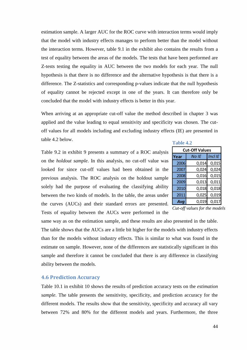
44

estimation sample. A larger AUC for the ROC curve with interaction terms would imply

that the model with industry effects manages to perform better than the model without

the interaction terms. However, table 9.1 in the exhibit also contains the results from a

test of equality between the areas of the models. The tests that have been performed are

Z-tests testing the equality in AUC between the two models for each year. The null

hypothesis is that there is no difference and the alternative hypothesis is that there is a

difference. The Z-statistics and corresponding p-values indicate that the null hypothesis

of equality cannot be rejected except in one of the years. It can therefore only be

concluded that the model with industry effects is better in this year.

When arriving at an appropriate cut-off value the method described in chapter 3 was

applied and the value leading to equal sensitivity and specificity was chosen. The cut-

off values for all models including and excluding industry effects (IE) are presented in

table 4.2 below.

Table 9.2 in exhibit 9 presents a summary of a ROC analysis

on the holdout sample. In this analysis, no cut-off value was

looked for since cut-off values had been obtained in the

previous analysis. The ROC analysis on the holdout sample

solely had the purpose of evaluating the classifying ability

between the two kinds of models. In the table, the areas under

the curves (AUCs) and their standard errors are presented.

Tests of equality between the AUCs were performed in the

same way as on the estimation sample, and these results are also presented in the table.

The table shows that the AUCs are a little bit higher for the models with industry effects

than for the models without industry effects. This is similar to what was found in the

estimate on sample. However, none of the differences are statistically significant in this

sample and therefore it cannot be concluded that there is any difference in classifying

ability between the models.

4.6 Prediction Accuracy

Table 10.1 in exhibit 10 shows the results of prediction accuracy tests on the estimation

sample. The table presents the sensitivity, specificity, and prediction accuracy for the

different models. The results show that the sensitivity, specificity and accuracy all vary

between 72% and 80% for the different models and years. Furthermore, the three

Table 4.2

Cut-off values for the models

Year No IE Incl IE

2006 0,014 0,015

2007 0,024 0,024

2008 0,016 0,015

2009 0,013 0,011

2010 0,018 0,018

2011 0,025 0,019

Avg 0,019 0,017

Cut-Off Values

45

measures are exactly the same for almost all models. This was expected since the cut-

off value was chosen where sensitivity and specificity were equal. Since the accuracy

measure is a weighted average of the two measures, all of the three measures will be

equal. However, on two of the models the sensitivity and specificity are not exactly the

same. The reason for these small differences is that the cut-off values were picked

manually and not through an automatic process. Sometimes it was difficult to pick the

exact cut-off value that lead to equality between sensitivity and specificity.

In addition to the three measures of classification accuracy, the table also contains the

results from a statistical test. The test performed tested the equality in prediction

accuracy between the models including and excluding industry effects. The alternative

hypothesis was that the prediction accuracy was greater for the models containing

industry effects. The results show that the null hypothesis can be rejected in four out of

six tests.

Table 10.2 in exhibit 10 shows the results from the tests of prediction accuracy on the

holdout samples. The table first shows the same measures as the table for the estimation

sample. Looking at the table, it is clear that the results differ. Here, sensitivity and

specificity are not equal, and this was also expected. The cut-off value was optimized to

make sensitivity and specificity equal in the estimation sample but random variation in

the samples makes it understandable that this exact equality will not hold when applying

the model on another sample.

Comparing the models with and without industry effects, the table shows that the

models with industry effects have a little bit higher sensitivity, specificity and prediction

accuracy than the ones without industry effects. To test for a difference, tests similar to

the ones performed on the estimation sample were done. However, as was discussed

previously, the mean of the sensitivity and specificity was here used as the evaluation

criterion. The results are presented in the right part of table 10.2 in exhibit 10 and are

varying just like the tests on the estimation sample. For three of the years, the model

with industry effects performs significantly better than the one without these effects.

46

5 DISCUSSION

The study has examined the predictive ability of financial ratios across industries and

time. The estimated models showed to be in line with the initial hypothesis. The model

contained all the kinds of financial variables that were expected. First of all, leverage

was assumed to be a good predictor. The relationship showed up to be positive in the

models which is a result supported by previous studies. The positive relationship is also

in line with the Merton Model that implies that a higher leverage increases the risk that

the firm value will fall below the default barrier.

Second, some measure of profitability was expected to be a good predictor. The

relationship is negative which is in line with the expectations based on the Merton

Model and previous studies. Lastly, after input from employees at Swedbank and its

appearance in previous research, liquidity was motivated to be a predictor. This variable

turned out to be a good predictor with a high marginal effect on bankruptcy each year.

This significant relationship can be interpreted as a sign of market inefficiencies. In a

perfect capital market, illiquidity itself should not be a reason for bankruptcy. However,

in the real world even a profitable company can go bankrupt if it does not have enough

liquidity and access to the capital markets for six months since a creditor can put a

company in bankruptcy within this time.

In addition to these three variables, the final model contained a fourth variable – a size

measure. Size showed to have a negative relationship with bankruptcy. These results are

in line with Ohlson’s (1980) study which also showed that size had a negative

relationship with bankruptcy. However, other ratios used in previous research did not

prove to be as good predictors. For example, Ohlson’s variable current assets/current

liabilities (or in this study its inverted form) was not good enough to be in the final

model of this study. Altman’s (1968) capital turnover variable is another example of a

variable that did not show to be a good predictor. One reason why these variables were

not as good in this study could be because a different population of companies was

studied. Another reason is of course the restriction made in this study to use only four

variables.

The hypotheses regarding industry differences that were formulated based on Chava &

Jarrow’s (2004) results are not supported in this study. The results showed to be

opposite to the expectations. The first hypothesis was that the manufacturing industry

47

should have a higher leverage coefficient than the transportation industry. In this study

however, the transportation industry has a higher coefficient on this ratio. This

unexpected difference is also statistically significant in three of the years. The second

hypothesis was that the transportation industry should be more sensitive to changes in

the return on total assets compared to the manufacturing industry. Also this hypothesis

was based on the results from Chava & Jarrow’s study and again the results in this study

indicate an opposite relationship. However, in this case the opposite relationship is only

statistically significant in one of the six years. One reason for these differences could be

that the industry classifications are slightly different. In Chava & Jarrow’s study,

transportation and utility companies are for example pooled together into one category.

Another reason could be because the studies are performed in different countries and on

data from completely different time periods. The industries have developed over time

and probably also their average financial ratios which could be the reason for the

models to change.

On average only five interaction terms accounting for industry effects showed to be

significant in each year which is less than what was expected initially. This average

number is also a little bit lower than the number of significant industry-variables Chava

& Jarrow (2004) found, despite using much more variables in the models of this study.

One reason why their study found more significant variables could be because their

models were adapted to large, public companies. These companies probably have more

reliable financial data because of the more strict regulations they are facing. This study

on the other hand has examined companies of all different sizes and conditions and

there is therefore probably a larger dispersion within the industry categories which

makes them less distinct.

The results from the analysis of the classification abilities of the models are varying.

The ROC analysis showed that no statistically significant difference could be found

between the models with and without industry effects. However, the analysis of the

prediction accuracy using specific cut-off values shows that the models incorporating

industry differences in three cases perform better than the ones without industry effects.

These latter results are in line with Chava & Jarrow’s (2004) and Platt & Platt’s (1990)

studies where they also found that models incorporating industry effects perform better.

48

More specifically, the prediction accuracy is on average 76.5% for the models without

industry effects and 77.7% for the models with industry effects when applied on the

holdout sample. These results are not as good as Beaver’s (1966), Altman’s (1968) or

Ohlson’s (1980) results of up to 87%, 82%-94% and 85.1% respectively. One possible

reason for the different results was discussed above. The argument was that the previous

studies are based on large public companies whose financial data may be more reliable

and less dispersed. This could make the classification easier. What is particularly

interesting in the comparison with the previous studies is that the industry-adapted

models in this study that are containing 25 terms did not get as good prediction accuracy

as one single financial ratio in Beaver’s study. Clearly, one can question the use of

advanced prediction models in the light of these results.

49

6 CONCLUSION

This chapter presents a conclusion of this study and a final discussion on the study’s

results. The goal is to answer the stated research questions and to fulfill the purpose of

the thesis.

6.1 Conclusions

The purpose of this study has been to examine the ability of different financial ratios to

predict corporate bankruptcy across industries and time. The study found four financial

variables that were able to predict bankruptcy and which the analysis was concentrated

to.

First, logistic regression models both excluding and including industry effects were

estimated for each year between 2006 and 2011. The models were then analyzed for

differences between the years and industries. Leverage and size showed a decreasing

trend over the years, and statistical tests showed that there was a statistically significant

difference between their coefficients for 2006 and 2011. From this analysis, it can be

concluded that the variation in marginal effect on bankruptcy over time for the two

variables leverage and size is statistically significant. However, also the coefficients for

the other variables varied a lot, and tests between other combinations of years may

therefore show other results.

The implications of the results are that bankruptcy prediction models vary depending on

the time of the estimation. Therefore it can be concluded that bankruptcy prediction

models preferably should be used on company data from the same time period as it was

estimated. However, as was discussed earlier, a bankruptcy prediction model can only

be estimated in retrospect. This leads to that one can question the use of these kinds of

models. One can especially question the common practice of pooling data from many

years in a static model since two of the variables showed to have a trend which makes

older data less relevant than more recent one.

Differences were not only found across time but also across industries. The analysis

showed that different financial ratios where significant for different industries. For

example, for some of the industries, the return on total assets ratio did not have any

significant marginal effect on bankruptcy. Some of the other differences across

industries that were found were for example that leverage has a higher marginal effect

50

on bankruptcy for the transportation industry compared to the manufacturing industry

and that the liquidity ratio has a lower marginal effect on bankruptcy for the hotel and

restaurant industry. However not many of the industry differences were significant.

The estimated models were also tested. The tests showed that the performance of the

models was relatively low compared to previous studies. The tests also showed that

including the industry effects in the model increased the classifying ability, sensitivity

and specificity only a little bit in the tested samples. When different tests of equality

between the models were performed, the results were ambiguous. The tests of equality

in the area under the ROC showed that no differences were statistically significant on

the holdout sample. However, when a test of equality between the mean of the

sensitivity and specificity for the two models was performed, the difference was

significant in three out of six years. In these three years the accuracy was increased by

incorporating the industry differences.

The ambiguity between the two tests makes it harder to draw any conclusions. Yet, by

looking at the definitions of the measures, some differences can be found. While the

area under the ROC curve is a measure of the classifying ability of a model regardless

any specific cut-off value, the mean of the sensitivity and specificity is a measure of

classification accuracy using a specific cut-off value. Therefore it cannot be concluded

that there exist any difference in classifying ability for the two models regardless cut-off

value but that it does exist a difference when using these specific cut-off values in three

of the six years.

6.2 Suggestions for Further Research

This study set out to answer questions regarding industry effects on bankruptcy

prediction. Although the stated questions have been answered, new ones have surfaced

along the way.

In the interaction with Swedbank it became obvious that much more than accounting

data is considered when evaluating a company. Future research could therefore try a

new perspective on a broader range of variables and not only financial variables to make

the bankruptcy prediction models more successful. Such variables can be for example

the private economy of the CEO or the change of board members.

51

The results in this study show that the bankruptcy prediction models vary over time.

However, there are still questions about how the variation is connected to

macroeconomic factors. An interesting angle would therefore be to analyze the

macroeconomic effects on the model and see if an incorporation of these effects in the

model can increase the performance.

In this study only five industries have been studied. Future research on the subject could

therefore analyze other industries and choose another methodology in this industry

selection. It would for example be interesting to choose the most dissimilar industries in

some way in an attempt to make the industry-adaptation in the model more relevant.

One question that has surfaced during this study is what effects different corporate rules

and regulations have on the predictive ability of financial ratios. Does the performance

of a prediction model vary across countries because of such differences? One idea

would be to exchange the industry dummies in this study for country dummies if these

differences would appear to be large.

52

REFERENCES

Articles

Al-Sulaiti, K. I. & Almwajeh, O. (2007). Applying Altman Z-Score Model of

Bankruptcy on Service Organizations and its Implications on Marketing Concepts and

Strategies. Journal of International Marketing & Marketing Research, 32, (2), 59-74.

Altman, E. (1968). Financial Ratios. Discriminant analysis and the prediction of

corporate bankruptcy. The Journal of finance, 23, (4), 589-609.

Altman, E. (2000). Predicting Financial Distress of Companies: Revisiting the Z-score

and Zeta Models. Personal Homepage, July.

Altman, E. (2002). Corporate Distress Prediction Models in a Turbulent Economic and

Basel II Environment. Personal Homepage, September.

Anderson, R. W., & Sundaresan, S. (1996). Design and valuation of debt contracts.

Review of Financial Studies, 9, (1), 37-68.

Anderson, R. W., Sundaresan, S., & Tychon, P. (1996). Strategic Analysis of

Contingent Claims. European Economic Review, 40, (3-5), 871-881.

Beaulieu, P. (1996). A Note on the Role of Memory in Commercial Loan Officer’s

Accounting and Character Information. Accounting, Organizations and Society, 21, (6),

515-528.

Beaver, W. H. (1966). Financial Ratios as Predictors of Failure. Journal of Accounting

Research, 4, (3), 71-111.

Black, F., & Cox, J. (1976). Valuating corporate securities: Some effects of bond

indenture Provision. The journal of Finance, 31, (2), 351-367.

Black, F., & Scholes, M. (1973). The Pricing of Options and Corporate Liabilities.

Journal of Political Economy, 81, (3), 637-654.

Brambor, T., Clark, W. R., & Golder, M. (2006). Understanding Interaction Models:

Improving Empirical Analyses. Political Analysis, 14, (1), 63-82.

Collin-Dufresne, P. & Goldstein, P. S. (2001). Do Credit Spreads Reflect Stationary

Leverage Ratios?. The Journal of Finance, 56, (5), 1929-1957.

53

Covitz, D. M., & Harrison, P. (2003). Testing Conflicts of Interest at Bond Ratings

Agencies with Market Anticipation: Evidence that Reputation Incentives Dominate.

Board of Governors of the Federal Reserve System (U.S.). Working Paper No. 68.

Chava, S. & Jarrow, R. A. (2004). Bankruptcy Prediction with Industry Effects. Review

of Finance, 8, (4), 537-569.

Dakovic, R., Czado, C., & Berg, D. (2010). Bankruptcy Prediction in Norway: A

Comparison Study. Applied Economics Letters, 17, (17), 1739-1746.

Deakin, E. B. (1972). “A Discriminant Analysis of Predictors of Business Failure”.

Journal of Accounting Research, 10, (1), 167-179.

Eisenbeis, R. (1977). Pitfalls in the Application of Discriminant Analysis in Business,

Finance, and Economics. Journal of Finance, 32, (3), 875-900.

Fawcett, T. (2006). An Introduction to ROC Analysis. Pattern Recognition Letters, 27,

(8), 861-874.

Frost, C. A. (2007). Credit Rating Agencies in Capital Markets: A Review of Research

Evidence on Selected Criticisms of the Agencies. Journal of Accounting, Auditing &

Finance, 22, (3), 469-492.

Hillegeist, S. A., Keating, E. K., Cram, D. P., & Lundstedt, K. G. (2004). Assessing the

Probability of Bankruptcy. Review of Accounting Studies, 9, (1), 5-34.

Karaca-Mandic, P., Norton, E. C., & Dowd, B. (2012). Interaction Terms in Nonlinear

Models. Health Services Research, 47, (1), 255-274.

Kim, H. & Gu, Z. (2006). Predicting Restaurant Bankruptcy: A Logit Model in

Comparison with a Distriminant Model. Journal of Hospitality and Tourism Research,

30, (4), 474-493.

Kim, S. Y. (2011). Prediction of Hotel Bankruptcy using Support Vector Machine,

Artificial Neural Network, Logistic Regression, and Multivariate Discriminant

Analysis. The Service Industries Journal, 31, (3), 441-468.

54

Mensah, Y. (1984). An Examination of the Stationarity of Multivariate Bankruptcy

Prediction Models: A Methodological Study. Journal of Accounting Research, 22, (1),

380-395.

Merton, R. C. (1974). On the Pricing of Corporate Debt: The Risk Structure of Interest

rates. The Journal of Finance, 29, (2), 449-470.

Ng, S. T., Wong, J. M. W., & Zhang, J. (2011). Applying Z-score Model to Distinguish

Insolvent Construction Companies in China. Habitat International, 35, (4), 599-607.

Ohlson, J. (1980). Financial Ratios and the Probabilistic Prediction of Bankruptcy.

Journal of Accounting Research, 18, (1), 109-131.

Platt H. D. & Platt M. B. (1990). Development of a class of stable predictive variables:

The case of bankruptcy prediction. Journal of Business Finance & Accounting, 17,(1),

31-51

Pendharkar, P. (2011). Probabilistic Approaches for Credit Screening and Bankruptcy

Prediction. Intelligent Systems in Accounting, Finance and Management, 18, (4), 177-

193.

Skogsvik, K. (1990). Current Cost Accounting Ratios as Predictors of Business Failure:

The Swedish Case. Journal of Business Finance & Accounting, 17, (1), 137-160.

Taffler, R. J. (1982). Forecasting Company Failure in the UK Using Discriminant

Analysis and Financial Ratio Data. Journal of the Royal Statistical Society, 145, (3),

342-358.

Vasicek, O. A. (1977). An Equilibrium Characterization of the Term Structure. Journal

of Financial Economics, 5, (2), 177-188

Yip, P. S. L. & Tsang, E. W. K. (2007). Interpreting Dummy Variables and their

Interaction Effects in Strategy Research. Strategic Organization, 5, (1), 13-30.

Books

A Dictionary of Finance and Banking. (2008). Oxford: Oxford University Press.

BAS. (2010). BAS Nyckeltal – för bättre analys och effektivare ekonomistyrning.

Stockholm: Norstedts Juridik.

55

Bryman, A. & Bell, E. (2005). Företagsekonomiska Forskningsmetoder (B. Nilsson

Trans.). Malmö: Liber Ekonomi. (Original work published 2003)

Charitou, A., Lambertides, N., & Trigeorgis, L. (2008). Bankruptcy Prediction and

Structural Credit Risk Models. In S. Jones (Ed) & D. A. Hensher (Ed), Advances in

Credit Risk Modelling and Corporate Bankruptcy Prediction (pp. 154-174). Cambridge:

Cambridge University Press.

Gray, D. & Malone, S. W. (2008). Macrofinancial Risk Analysis. Chichester: J. Wiley

& Sons Ltd

Gregow, T. (2011). Sveriges Rikes Lag. Stockholm: Norstedts Juridik.

Hair, J. F. Jr., Black, W. C., Babin, B. J., & Anderson, R. E. (2010). Multivariate Data

Analysis (7th

edition). Upper Saddle River, NJ: Pearson Education, Inc.

Han, J. & Kamber, M. (2006). Data Mining, Concepts and Techniques (2nd

edition). San

Francisco, CA: Morgan Kaufmann Publishers.

Körner, S. & Wahlgren, L. (2009). Statistisk Dataanalys. Lund: Studentlitteratur.

Schumpeter, J. A. (1942). Capitalism, Socialism and Democracy. New York & London:

Harper & Brothers.

Tan, P. N., Steinbach, M., & Kumar, V. (2005). Introduction to Data Mining. Upper

Saddle River, NJ: Pearson Education, Inc.

Internet Sources

Brandow Company. (2013). BizStats. [Online] Available at http://www.bizstats.com/

[Used February 25]

Cecilia Vinell. (2011, September 19). Därför bör du ha koll på nyckeltalen. [Online]

Available at http://www.ekonomisverige.se/nyheter/darfor-bor-du-ha-koll-pa-

nyckeltalen/ [Used March 10 2013]

Quantitative Micro Software, LLC. (2009). Eviews 7, Users Guide II. [Online]

Available at http://schwert.ssb.rochester.edu/a425/EV72.pdf [Used April 16 2013]

56

Retriever AB. (2009). Retriever User Guide. [Online] Available at http://web.retriever-

info.com.ludwig.lub.lu.se/static/pdf/businessinfo/businessinfo_manual_090930_v2.pdf

[Used March 6 2013]

Retriever AB. (2013). Retriever Business. [Online] Available at http://www.retriever-

info.com/se [Used January 15 to March 20]

The Swedish Agency for Growth Policy Analysis. (2013). Tillväxtanalys – Statistik över

konkurser. [Online] Available at http://www.tillvaxtanalys.se/ [Used April 25 2013]

57

Code Name Definition

SOLID Solidity Adjusted equity as % of total assets

LEV Leverage Total liabilities/total assets

CAPTO Capital turnover ratio Net turnover/total assets

WCAPSA Working capital in

relation to turnover

Working capital as % of net turnover

WCAPTA Working capital in

relation to total assets

Working capital as % of total assets

STDSA Short-term debt in

relation to turnover

Short-term debt as % of net turnover

RECSA Receivables in relation to

turnover

Receivables as % of net turnover

LIQSTD Cash liquidity Current assets excluding inventory etc,

as % of short-term debt

LIQSA Liquidity in relation to

turnover

Liquidity/turnover

LIQTA Liquidity in relation to

total assets

Liquidity/total assets

INVSA Inventory and ongoing

activity etc over sales

Inventory and ongoing activity etc as

% of net turnover

INVTO Inventory turnover rate Cost of goods sold/average inventory

CHSA Change in sales Difference between t and t-1 net

turnover, as a % of t-1 net turnover

LOGTA Log total assets Ln(total assets)

Development

Firm Size

List and Explanation of Collected Financial Ratios (Cont'd)

Capital Structure

Code Name Definition

R_E Return on equity Net income/adjusted equity

R_TA Return on total capital Operating profit + fin incomes as % of

total assets

INTD Interest on debt Fin. expenses/sum of appropriation &

debt including suspended tax debt

RMG Risk margin on total

capital

Difference in % between return on

total capital and interest on debt

R_OPC Return on operating

capital

Operating profit + fin income as % of

operating capital

OPRMG Operating Risk margin Difference (%) in return on operating

capital and interst rate

OPMG Operating margin Operating profit as % of net turn-over

PRMG Profit margin Net income as % of net turn-over

INTCOV Interest coverage Operating profit including fin revenues/

fin. costs

OPPREMPL Operating profit per

employee

Operating profit after ammortization/

average number of employees

SAEMPL Net sales per employee Net turnover/avg number of employees

CEMPL Cost per employee tkr Employee costs/avg number of

employees

List and Explanation of Collected Financial Ratios

Return Structure

Profit Structure

Income/Cost Structure

Exhibit 1 – List of Financial Ratios

Table 1.1 Table 1.1, continued

58

Exhibit 2 – Bankruptcies across Industries

Table 2.1

Count

% Row

INDUSTRY SECTOR 2006 2007 2008 2009 2010 2011

NON-

BANKRUPT BANKRUPT TOTAL

Uncategorized 239 301 545 524 113 1 2557 1723 4280

44,51% 47,63% 58,98% 54,47% 18,05% 0,17% 59,74% 40,26% 100%

Sewer, Waste, Electricity and Water 0 1 2 1 0 1 3000 5 3005

0% 0,22% 0,42% 0,20% 0% 0,17% 99,83% 0,17% 100%

Staffing and Employment Agencies 2 13 13 1 15 16 2543 60 2603

0,75% 3,89% 3,35% 0,23% 2,82% 2,47% 97,69% 2,31% 100%

Industry and Employer Organizations 0 0 0 0 0 0 392 0 392

0,00% 0,00% 0,00% 0,00% 0,00% 0,00% 100,00% 0,00% 100,00%

Building, Design, & Decoration Businesses 72 155 113 89 151 190 48386 770 49156

1,14% 2,22% 1,46% 1,08% 1,64% 1,78% 98,43% 1,57% 100,00%

Data, IT & Telecom 12 23 8 6 18 11 11094 78 11172

0,91% 1,51% 0,46% 0,31% 0,83% 0,44% 99,30% 0,70% 100,00%

Retail 37 74 54 41 82 98 29827 386 30213

0,92% 1,68% 1,14% 0,80% 1,45% 1,57% 98,72% 1,28% 100,00%

Real Estate 40 72 60 56 50 16 14939 294 15233

2,03% 3,27% 2,49% 2,15% 1,75% 0,50% 98,07% 1,93% 100,00%

Business Services 9 27 8 4 23 19 6065 90 6155

1,16% 3,10% 0,84% 0,38% 1,97% 1,43% 98,54% 1,46% 100,00%

Health Care 5 14 5 10 12 11 9097 57 9154

0,47% 1,17% 0,37% 0,63% 0,66% 0,51% 99,38% 0,62% 100,00%

Hair & Beauty 3 2 1 0 1 3 1239 10 1249

2,27% 1,20% 0,52% 0,00% 0,40% 1,01% 99,20% 0,80% 100,00%

Hotels & Restaurants 45 82 52 43 57 44 18569 323 18892

2,05% 3,23% 1,83% 1,34% 1,52% 1,01% 98,29% 1,71% 100,00%

Agriculture, Forestry, Hunting & Fishing 2 13 5 5 6 9 6181 40 6221

0,25% 1,45% 0,51% 0,47% 0,52% 0,68% 99,36% 0,64% 100,00%

Legal, Business and Consulting Services 7 13 13 1 13 4 10060 51 10111

0,60% 0,97% 0,84% 0,06% 0,66% 0,17% 99,50% 0,50% 100,00%

Culture & Entertainment 6 4 1 0 8 2 3511 21 3532

1,31% 0,79% 0,18% 0,00% 1,22% 0,26% 99,41% 0,59% 100,00%

Food Production 8 10 3 1 14 13 4809 49 4858

1,15% 1,37% 0,39% 0,12% 1,59% 1,36% 98,99% 1,01% 100,00%

Media 1 4 0 1 6 5 2933 17 2950

0,26% 0,91% 0,00% 0,20% 1,09% 0,83% 99,42% 0,58% 100,00%

Motor Vehicle Dealing 2 5 0 1 6 5 4036 19 4055

0,33% 0,79% 0,00% 0,15% 0,83% 0,65% 99,53% 0,47% 100,00%

Public Administration 0 0 0 0 0 0 96 0 96

0,00% 0,00% 0,00% 0,00% 0,00% 0,00% 100,00% 0,00% 100,00%

Other Consumer Services 2 0 1 1 4 3 1485 11 1496

1,17% 0,00% 0,46% 0,39% 0,33% 0,81% 99,26% 0,74% 100,00%

Wholesale 16 53 23 4 59 53 35103 208 35311

0,32% 0,98% 0,40% 0,07% 0,93% 0,78% 99,41% 0,59% 100,00%

Advertisement and PR 7 17 10 6 19 24 4739 83 4822

1,17% 2,50% 1,31% 0,75% 2,10% 2,23% 98,28% 1,72% 100,00%

Reparation & Installation 6 13 11 5 11 24 8448 70 8518

0,53% 1,04% 0,82% 0,35% 0,70% 1,35% 99,18% 0,82% 100,00%

Travel Agencies & Tourism 2 5 1 1 1 3 1363 13 1376

1,08% 2,45% 0,46% 0,43% 0,39% 1,07% 99,06% 0,94% 100,00%

Technical Consulting 4 8 4 1 13 13 6048 43 6091

0,53% 0,95% 0,42% 0,10% 1,11% 1,16% 99,29% 0,71% 100,00%

Manufacturing 34 96 55 38 87 109 45166 419 45585

0,50% 1,34% 0,73% 0,50% 1,09% 1,28% 99,08% 0,92% 100,00%

Transportation & Storage 31 68 69 46 73 68 21485 355 21840

1,04% 2,08% 1,97% 1,25% 1,82% 1,54% 98,37% 1,63% 100,00%

Education, Research and Development 6 9 5 0 9 17 6649 46 6695

0,74% 1,00% 0,49% 0,00% 0,69% 1,14% 99,31% 0,69% 100,00%

Leasing 2 4 2 1 3 4 2110 16 2126

0,71% 1,32% 0,60% 0,29% 0,75% 0,86% 99,25% 0,75% 100,00%

Total 600 1086 1064 887 854 766 311930 5257 317187

1,43% 2,35% 2,11% 1,64% 1,45% 1,16% 98,34% 1,66% 100,00%

Number of Bankruptcies per Year Total number of observations

59

Exhibit 3 – Univariate Analysis

Table 3.1

Results from Univariate Analysis

Bankrupt Firms Non-bankrupt Firms Test for Equality of

Means

Variable Mean Std. Dev. Mean Std. Dev. T-statistic Prob.

CAPTO 3.836845 4.517157 2.770288 2.228241 -15.72162 0.0000

CEMPL 358.2010 121.2354 414.2719 134.7106 13.98054 0.0000

CHSA 254.2236 5861.756 120.3419 11103.12 -0.406508 0.6844

INVSA 7.944917 14.03755 8.184782 21.63113 0.373464 0.7088

INVTO 4.676345 55.40156 10.39976 176.8127 1.092656 0.2745

LEV 1.080848 0.722997 0.664630 0.460936 -29.98860 0.0000

LIQSA 2.718817 11.35666 10.21879 46.59154 5.435154 0.0000

LIQSTD 80.59738 173.6995 135.2942 135.6379 13.46744 0.0000

LIQTA 0.078033 0.131240 0.183870 0.193750 18.39261 0.0000

LOGTA 8.120192 1.185970 9.009671 1.414194 21.14153 0.0000

OPMG -6.100736 20.79664 2.901071 118.3873 2.567857 0.0102

OPPREMPL -49.13155 174.6787 84.07490 230.0721 19.47841 0.0000

PRMG -5.689895 20.53129 3.353799 118.0031 2.588217 0.0096

R_E -143.5224 1177.598 16.77627 868.6558 6.154575 0.0000

R_OPC -10.46414 1129.321 27.66481 2640.780 0.487087 0.6262

R_TA -17.32813 65.85460 9.918002 24.24930 36.13088 0.0000

RECSA 8.886161 10.15290 9.832895 19.91617 1.602774 0.1090

SAEMPL 1248.840 1189.504 1738.360 2044.841 8.067216 0.0000

SOLID -8.273392 73.73490 33.55036 39.72009 34.73817 0.0000

STDSA 30.51974 29.44296 23.29120 70.22046 -3.472902 0.0005

WCAPSA -4.511788 28.06559 9.182347 75.06895 6.155869 0.0000

WCAPTA -0.160505 0.708506 0.172803 0.401295 27.46208 0.0000

The table shows the mean and standard deviation on 22 different financial variables for

bankrupt and non-bankrupt companies in the estimation sample. The table also shows

the results from tests of equality between the two groups. The null hypothesis is that

there is no difference between the means for bankrupt and non-bankrupt companies.

The alternative hypothesis is that there is a difference.

60

Exhibit 4 – Financial Ratios across Industries

Table 4.1

Table 4.1, continued

The table contains the 17 financial variables that passed the previous univariate test. The table shows the mean of the financial variables for

bankrupt and non-bankrupt companies in the estimation sample, belonging to the five selected industries. The table also split up the five

industries and shows the means for each industry respectively.

Note: NB=Mean of non-bankrupt firms

B=Mean of bankrupt firms

NB B NB B NB B NB B NB B NB B NB B NB B NB B

Building 2.71 3.98 444 382 0.66 1.04 11.2 2.4 153.9 89.7 0.22 0.08 8.72 8.02 0.05 -0.02 90.3 -13.5

Hotel & Restaurant 3.55 4.93 317 259 0.80 1.39 9.7 4.0 112.8 62.5 0.25 0.14 8.12 7.27 0.02 -0.11 34.4 -46.5

Manufacturing 1.90 2.33 443 394 0.61 1.03 10.9 2.9 146.3 72.0 0.13 0.03 9.72 8.85 0.01 -0.23 113.9 -76.0

Retail 4.22 4.76 374 343 0.66 1.07 7.6 3.4 103.7 53.4 0.21 0.08 8.82 8.18 0.01 -0.11 71.2 -96.2

Transport 2.12 2.78 429 383 0.71 1.10 11.5 1.9 130.4 92.0 0.15 0.05 9.25 8.39 0.04 -0.02 81.6 -33.7

All 2.78 3.75 414 360 0.67 1.10 10.3 2.9 134.9 76.7 0.19 0.08 9.01 8.15 0.03 -0.09 85.9 -47.2

OPPREMPLCAPTO CEMPL LEV LIQSA LIQSTD LIQTA LOGTA OPMG

NB B NB B NB B NB B NB B NB B NB B NB B

Building 0.06 -0.02 0.32 -0.40 0.13 -0.10 1398 1160 34.3 -4.2 22.7 28.4 11.2 -1.4 0.23 -0.09

Hotel & Restaurant 0.03 -0.11 0.04 -0.87 0.06 -0.37 883 821 20.0 -38.8 22.5 31.6 -2.8 -13.3 -0.06 -0.50

Manufacturing 0.02 -0.22 0.11 -0.92 0.09 -0.19 1748 920 38.8 -2.9 27.7 57.8 14.0 -17.5 0.22 -0.09

Retail 0.02 -0.10 0.19 -3.27 0.10 -0.18 2487 4464 34.3 -6.7 17.5 32.8 9.7 -3.5 0.22 -0.04

Transport 0.05 -0.02 0.07 -0.11 0.07 -0.08 1921 903 29.5 -10.2 26.4 27.9 1.4 -10.7 0.01 -0.24

All 0.03 -0.08 0.18 -1.01 0.10 -0.17 1722 1575 33.3 -10.3 23.6 35.0 8.8 -7.9 0.17 -0.16

STDSA WCAPSA WCAPTAPRMG R_E R_TA SAEMPL SOLID

61

Exhibit 5 – Correlations among Financial Ratios

Table 5.1

The table shows the correlations among the remaining financial variables, based on companies from the five selected industries in the estimation

sample.

CAPTO

CEMPL

LEV

LIQSA

LIQST

D

LIQTA

LOGTA

OPMG

OPPREM

PL

PRMG

R_ER_TA

SAEM

PL

SOLID

STDSA

WCAPSA

WCAPTA

CAPTO 1.00 -0.11 0.24 -0.08 -0.11 0.09 -0.37 0.00 -0.05 0.00 0.03 -0.06 0.15 -0.26 -0.10 -0.04 -0.16

CEMPL 1.00 -0.09 0.05 0.05 0.00 0.40 -0.02 0.12 -0.02 -0.00 0.05 0.34 0.09 0.05 0.00 0.05

LEV 1.00 -0.08 -0.21 -0.24 -0.13 -0.02 -0.08 -0.02 -0.01 -0.40 -0.02 -0.99 0.05 -0.11 -0.78

LIQSA 1.00 0.14 0.21 0.02 -0.50 -0.01 -0.48 -0.01 0.00 -0.02 0.09 0.32 0.52 0.09

LIQSTD 1.00 0.28 0.04 0.01 0.05 0.01 0.01 0.07 -0.00 0.23 -0.03 0.13 0.25

LIQTA 1.00 -0.19 0.01 0.06 0.01 0.03 0.22 -0.02 0.26 -0.04 0.12 0.35

LOGTA 1.00 0.01 0.13 0.01 -0.00 0.05 0.32 0.14 0.08 -0.00 0.00

OPMG 1.00 0.07 1.00 0.06 0.13 0.01 0.02 -0.39 -0.11 0.03

OPPREMPL 1.00 0.07 0.06 0.20 0.31 0.08 -0.04 0.03 0.07

PRMG 1.00 0.06 0.13 0.01 0.02 -0.38 -0.10 0.03

R_E 1.00 0.14 0.01 0.01 -0.05 0.03 0.02

R_TA 1.00 0.05 0.41 -0.07 0.04 0.38

SAEMPL 1.00 0.02 -0.02 -0.00 0.02

SOLID 1.00 -0.06 0.12 0.77

STDSA 1.00 -0.57 -0.10

WCAPSA 1.00 0.20

WCAPTA 1.00

62

Exhibit 6 – Prediction Models excluding Industry Effects

Table 6.1 – Prediction Models

The table shows the bankruptcy prediction models for each year that was estimated

without industry effects.

Table 6.2 – Test Statistics for the Models

The table shows the test statistics for the estimated prediction models without industry

effects.

Variable 2006 2007 2008 2009 2010 2011

Coefficient 1.5842 0.5149 1.2538 0.3777 0.0758 -0.1284

Std. Error 0.9204 0.6509 0.6800 0.7456 0.5579 0.4499

Z-Statistic 1.7213 0.7911 1.8437 0.5066 0.1359 -0.2855

P-value 0.0852 0.4289 0.0652 0.6125 0.8919 0.7753

Coefficient 0.9344 1.3289 0.5758 0.5138 0.3568 0.1776

Std. Error 0.2859 0.2179 0.1559 0.1681 0.1230 0.0422

Z-Statistic 3.2686 6.0997 3.6936 3.0568 2.9021 -4.2059

P-value 0.0011 0.0000 0.0002 0.0022 0.0037 0.0000

Coefficient -4.2609 -4.9960 -3.1251 -5.1100 -6.0922 -5.8321

Std. Error 0.8608 0.6841 0.5996 0.8044 0.7144 0.6202

Z-Statistic -4.9498 -7.3032 -5.2121 -6.3527 -8.5281 -9.4038

P-value 0.0000 0.0000 0.0000 0.0000 0.0000 0.0000

Coefficient -0.6271 -1.5396 -1.3422 -0.7721 -1.3474 -0.9212

Std. Error 0.4146 0.2912 0.2172 0.2269 0.2028 0.1699

Z-Statistic -1.5127 -5.2879 -6.1805 -3.4028 -6.6433 -5.4227

P-value 0.1304 0.0000 0.0000 0.0007 0.0000 0.0000

Coefficient -0.7447 -0.5647 -0.6439 -0.5570 -0.4491 -0.3733

Std. Error 0.1008 0.0677 0.0749 0.0821 0.0614 0.0521

Z-Statistic -7.3867 -8.3418 -8.5999 -6.7842 -7.3166 -7.1632

P-value 0.0000 0.0000 0.0000 0.0000 0.0000 0.0000

Annual Bankruptcy Prediction Models without Industry-Effects

LOGTA

Intercept

LEV

LIQTA

R_TA

2006 2007 2008 2009 2010 2011

LR Statistic 184.7916 412.0594 294.4631 205.6030 304.8784 240.0070

Prob(LR-Stat) 0.0000 0.0000 0.0000 0.0000 0.0000 0.0000

SEE 0.1002 0.1312 0.1156 0.0984 0.1189 0.1206

McFadden

R-Squared0.1454 0.1828 0.1537 0.1310 0.1311 0.0907

63

Table 6.3

The table shows equality tests on the different coefficients of the different variables in

the prediction models without industry effects. The tests test the equality in the

coefficients between 2006 and 2011.

Note:

Null-hypothesis: Coefficient for 2006=Coefficient for 2011

Alternative hypothesis: Coefficient for 2006≠Coefficient for 2011

Variable 2006 2011 Z-Statistic P-value

Intercept Coefficient 1.5842 -0.1284 1.6718 0.0946

Std. Error 0.9204 0.4499

LEV Coefficient 0.9344 0.1776 2.6187 0.0088

Std. Error 0.2859 0.0422

LIQTA Coefficient -4.2609 -5.8321 1.4809 0.1386

Std. Error 0.8608 0.6202

R_TA Coefficient -0.6271 -0.9212 0.6564 0.5116

Std. Error 0.4146 0.1699

LOGTA Coefficient -0.7447 -0.3733 -3.2727 0.0011

Std. Error 0.1008 0.0521

Test of Coefficient Equality between Years

64

Exhibit 7 – Prediction Models including Industry Effects

Table 7.1 Table 7.1, continued

Variable 2006 2007 2008 2009 2010 2011

Coefficient 4.2393 1.2297 -0.5933 -6.6985 -4.5119 -2.4208

Std. Error 2.9099 1.6048 1.9888 1.8219 1.2113 1.0728

Z Statis tic 1.4568 0.7663 -0.2983 -3.6767 -3.7249 -2.2566

P-value 0.1452 0.4435 0.7654 0.0002 0.0002 0.0240

Coefficient 1.2669 2.0295 2.2513 2.5687 1.4804 1.3687

Std. Error 0.7665 0.6744 0.7711 0.5524 0.4206 0.3667

Z Statis tic 1.6530 3.0093 2.9198 4.6503 3.5200 3.7325

P-value 0.0983 0.0026 0.0035 0.0000 0.0004 0.0002

Coefficient -11.8160 -23.3286 -4.4578 -2.7891 -9.5732 -7.7609

Std. Error 4.3583 6.7504 2.6458 2.6762 3.2042 2.2765

Z Statis tic -2.7112 -3.4559 -1.6849 -1.0422 -2.9877 -3.4091

P-value 0.0670 0.0005 0.0920 0.2973 0.0028 0.0007

Coefficient -2.7976 -2.6551 -0.9946 -1.1919 -1.7868 -1.0302

Std. Error 0.8839 0.7162 0.5398 0.6094 0.4718 0.3899

Z Statis tic -3.1652 -3.7074 -1.8424 -1.9558 -3.7872 -2.6424

P-value 0.0016 0.0002 0.0654 0.0505 0.0002 0.0082

Coefficient -1.1188 -0.6733 -0.6129 -0.0334 -0.0705 -0.2471

Std. Error 0.3216 0.1562 0.1954 0.1642 0.1138 0.1018

Z Statis tic -3.4788 -4.3100 -3.1368 -0.2034 -0.6195 -2.4282

P-value 0.0005 0.0000 0.0017 0.8389 0.5356 0.0152

Coefficient -1.2373 0.4080 -1.5521 -0.5326 -0.1832 -0.1087

Std. Error 0.8567 0.8545 0.8150 0.7490 0.5794 0.4796

Z Statis tic -1.4442 0.4775 -1.9044 -0.7111 -0.3163 -0.2265

P-value 0.1487 0.6330 0.0569 0.4771 0.7518 0.8208

Coefficient 1.4178 0.3434 -1.1605 -1.5024 -1.4038 -1.2464

Std. Error 1.5294 0.9432 0.9591 0.8663 0.4446 0.3757

Z Statis tic 0.9270 0.3641 -1.2100 -1.7343 -3.1577 -3.3175

P-value 0.3539 0.7158 0.2263 0.0829 0.0016 0.0009

Bankruptcy Prediction Models with Industry-Effects

LEV*

RETAIL

LEV*

BUILDING

Intercept

LEV

LIQTA

R_TA

LOGTA

Variable 2006 2007 2008 2009 2010 2011

Coefficient -0.3875 -1.3700 -2.3245 -2.5990 -1.3773 -1.6068

Std. Error 0.8701 0.7367 0.8262 0.6261 0.4892 0.3754

Z Statis tic -0.4453 -1.8598 -2.8135 -4.1510 -2.8152 -4.2805

P-value 0.6561 0.0629 0.0049 0.0000 0.0049 0.0000

Coefficient 6.3292 2.1787 3.1382 3.6150 1.3636 1.0831

Std. Error 1.7188 1.4776 1.4419 1.5451 0.9045 0.7703

Z Statis tic 3.6823 1.4745 2.1764 2.3397 1.5076 1.4061

P-value 0.0002 0.1403 0.0295 0.0193 0.1317 0.1597

Coefficient 7.6640 21.0810 1.4815 -1.0246 4.0801 2.1982

Std. Error 4.5876 6.8173 2.8010 2.9631 3.4008 2.5343

Z Statis tic 1.6706 3.0923 0.5289 -0.3458 1.1998 0.8674

P-value 0.0948 0.0020 0.5969 0.7295 0.2302 0.3857

Coefficient 4.2720 20.0313 3.1255 -5.7704 3.1768 3.7414

Std. Error 5.0663 6.9376 3.0547 3.8690 3.6351 2.5670

Z Statis tic 0.8432 2.8874 1.0232 -1.4914 0.8739 1.4575

P-value 0.3991 0.0039 0.3062 0.1358 0.3822 0.1450

Coefficient 10.7025 18.8219 3.3167 0.4120 0.8256 4.8891

Std. Error 4.5401 6.9150 2.8831 3.0174 3.7557 2.6794

Z Statis tic 2.3573 2.7219 1.1504 0.1365 0.2198 1.8247

P-value 0.0184 0.0065 0.2500 0.8914 0.8260 0.0680

Coefficient 3.0797 17.4399 1.0485 -5.1051 6.7454 4.1584

Std. Error 6.0381 7.1342 3.4947 4.4918 3.6090 2.9997

Z Statis tic 0.5101 2.4446 0.3000 -1.1365 1.8691 1.3863

P-value 0.6100 0.0145 0.7641 0.2557 0.0616 0.1657

Bankruptcy Prediction Models with Industry-Effects (cont'd)

LEV*HR

LEV*

TRANS

PORT

LIQTA*

BUILDING

LIQTA*

RETAIL

LIQTA*HR

LIQTA*

TRANS

PORT

65

Table 7.1, continued Table 7.1, continued

The table shows the estimated bankruptcy prediction models for each year with industry effects included.

Variable 2006 2007 2008 2009 2010 2011

Coefficient 0.6844 2.0514 -0.1375 0.4450 1.2457 -0.0377

Std. Error 1.2747 1.0395 0.6730 0.8603 0.6731 0.5230

Z Statis tic 0.5369 1.9734 -0.2043 0.5173 1.8508 -0.0720

P-value 0.5913 0.0484 0.8382 0.6049 0.0642 0.9426

Coefficient 4.1436 -1.1457 -2.5073 2.7591 0.0462 0.8168

Std. Error 1.6723 1.1225 0.8712 1.3061 0.6655 0.4039

Z Statis tic 2.4778 -1.0206 -2.8781 2.1124 0.0694 2.0224

P-value 0.0132 0.3074 0.0040 0.0346 0.9447 0.0431

Coefficient 2.7560 1.3659 -0.3400 -0.2926 1.0598 -0.0596

Std. Error 1.0152 0.8770 0.7074 0.7475 0.6462 0.5173

Z Statis tic 2.7148 1.5575 -0.4807 -0.3915 1.6399 -0.1152

P-value 0.0066 0.1194 0.6308 0.6955 0.1010 0.9083

Coefficient 1.3002 2.6283 -0.1829 1.6439 2.6881 1.2153

Std. Error 1.8980 1.4829 0.7358 1.4578 1.1433 0.7506

Z Statis tic 0.6851 1.7724 -0.2486 1.1277 2.3511 1.6191

P-value 0.4933 0.0763 0.8037 0.2595 0.0187 0.1054

Coefficient 0.6556 0.2154 -0.1060 -0.6502 -0.4058 0.0047

Std. Error 0.3670 0.1999 0.2425 0.2325 0.1683 0.1402

Z Statis tic 1.7862 1.0778 -0.4374 -2.7961 -2.4119 0.0337

P-value 0.0741 0.2811 0.6618 0.0052 0.0159 0.9731

Coefficient 0.5219 0.1147 0.0845 -0.4226 -0.7947 0.0913

Std. Error 0.4147 0.2522 0.2912 0.2923 0.2413 0.1633

Z Statis tic 1.2584 0.4550 0.2901 -1.4456 -3.2938 0.5591

P-value 0.2082 0.6491 0.7717 0.1483 0.0010 0.5761

R_TA*

TRANS

PORT

LOGTA*

BUILDING

LOGTA*

RETAIL

Bankruptcy Prediction Models with Industry-Effects (cont'd)

R_TA*

BUILDING

R_TA*

RETAIL

R_TA*HR

Variable 2006 2007 2008 2009 2010 2011

Coefficient 0.4480 0.1437 -0.1287 -0.2061 -0.4201 -0.2856

Std. Error 0.3993 0.2449 0.3088 0.2602 0.1910 0.2502

Z Statis tic 1.1220 0.5867 -0.4168 -0.7922 -2.1999 -1.1416

P-value 0.2619 0.5574 0.6768 0.4283 0.0278 0.2536

Coefficient 0.0955 -0.1498 0.0504 -0.6366 -0.2961 -0.0765

Std. Error 0.4443 0.2491 0.2613 0.2822 0.1980 0.1959

Z Statis tic 0.2148 -0.6013 0.1929 -2.2558 -1.4959 -0.3906

P-value 0.8299 0.5476 0.8471 0.0241 0.1347 0.6961

Coefficient -4.0555 -2.6401 2.5540 6.9026 4.1042 0.1758

Std. Error 3.2831 1.9849 2.3516 2.3580 1.6770 1.4241

Z Statis tic -1.2353 -1.3300 1.0861 2.9273 2.4473 0.1234

P-value 0.2167 0.1835 0.2774 0.0034 0.0144 0.9018

Coefficient -5.1290 -1.8713 -0.0821 5.7584 8.0601 0.0917

Std. Error 3.8841 2.4684 2.8200 2.9063 2.1716 1.5744

Z Statis tic -1.3205 -0.7581 -0.0291 1.9813 3.7116 0.0582

P-value 0.1867 0.4484 0.9768 0.0476 0.0002 0.9536

Coefficient -3.5295 -0.6426 2.4731 4.6868 5.5485 2.4512

Std. Error 3.5047 2.2554 2.7538 2.5179 1.7717 2.0463

Z Statis tic -1.0071 -0.2849 0.8981 1.8614 3.1317 1.1979

P-value 0.3139 0.7757 0.3691 0.0627 0.0017 0.2310

Coefficient -5.5270 -0.7405 -2.4053 3.6764 1.7772 -0.6474

Std. Error 4.1760 2.5623 2.8887 3.1134 2.1941 2.0696

Z Statis tic -1.3235 -0.2890 -0.8327 1.1808 0.8100 -0.3128

P-value 0.1857 0.7726 0.4050 0.2377 0.4180 0.7544

TRANS

PORT

Bankruptcy Prediction Models with Industry-Effects (cont'd)

LOGTA*HR

LOGTA*

TRANS

PORT

BUILDING

RETAIL

HR

66

Table 7.2 – Test Statistics for the Models

The table shows the test statistics for the estimated prediction models including industry effects.

2006 2007 2008 2009 2010 2011

LR Statistic 251.0263 490.7448 392.0353 309.5832 367.2819 359.1553

Prob(LR-Stat) 0.0000 0.0000 0.0000 0.0000 0.0000 0.0000

SEE 0.0985 0.1302 0.1133 0.0967 0.1177 0.1200

McFadden

R-Squared0.1975 0.2177 0.2046 0.1972 0.1579 0.1357

67

Exhibit 8 – Total Marginal Effects for Each Industry

Table 8.1 – Manufacturing Industry Table 8.2 – Building Industry

Variable 2006 2007 2008 2009 2010 2011

Intercept

Coefficient 4.2393 1.2297 -0.5933 -6.6985 -4.5119 -2.4208

Std Error 2.9099 1.6048 1.9888 1.8219 1.2113 1.0728

Z-Statistic 1.4568 0.7663 -0.2983 -3.6767 -3.7249 -2.2566

P-Value 0.1452 0.4435 0.7654 0.0002 0.0002 0.0240

LEV

Coefficient 1.2669 2.0295 2.2513 2.5687 1.4804 1.3687

Std Error 0.7665 0.6744 0.7711 0.5524 0.4206 0.3667

Z-statistic 1.6530 3.0093 2.9198 4.6503 3.5200 3.7325

P-Value 0.0983 0.0026 0.0035 0.0000 0.0004 0.0002

LIQTA

Coefficient -11.8160 -23.3286 -4.4578 -2.7891 -9.5732 -7.7609

Std Error 4.3583 6.7504 2.6458 2.6762 3.2042 2.2765

Z-statistic -2.7112 -3.4559 -1.6849 -1.0422 -2.9877 -3.4091

P-Value 0.0670 0.0005 0.0920 0.2973 0.0028 0.0007

R_TA

Coefficient -2.7976 -2.6551 -0.9946 -1.1919 -1.7868 -1.0302

Std Error 0.8839 0.7162 0.5398 0.6094 0.4718 0.3899

Z-statistic -3.1652 -3.7074 -1.8424 -1.9558 -3.7872 -2.6424

P-Value 0.0016 0.0002 0.0654 0.0505 0.0002 0.0082

LOGTA

Coefficient -1.1188 -0.6733 -0.6129 -0.0334 -0.0705 -0.2471

Std Error 0.3216 0.1562 0.1954 0.1642 0.1138 0.1018

Z-statistic -3.4788 -4.3100 -3.1368 -0.2034 -0.6195 -2.4282

P-Value 0.0005 0.0000 0.0017 0.8389 0.5356 0.0152

Total Marginal Effects, Manufacturing Industry

Variable 2006 2007 2008 2009 2010 2011

Intercept

Coefficient 0.1838 -1.4103 1.9607 0.2040 -0.4078 -2.2451

Std Error 1.5202 1.1682 1.2549 1.4970 1.1598 0.9366

Z-Statistic 0.1209 -1.2073 1.5624 0.1363 -0.3516 -2.3971

P-Value 0.9038 0.2273 0.1182 0.8916 0.7252 0.0165

LEV

Coefficient 0.0297 2.4375 0.6992 2.0362 1.2971 1.2601

Std Error 0.3828 0.5247 0.2640 0.5058 0.3985 0.3092

Z-statistic 0.0775 4.6458 2.6483 4.0257 3.2550 4.0758

P-Value 0.9382 0.0000 0.0081 0.0001 0.0011 0.0000

LIQTA

Coefficient -4.1520 -2.2476 -2.9763 -3.8137 -5.4931 -5.5627

Std Error 1.4323 0.9526 0.9195 1.2720 1.1396 1.1136

Z-statistic -2.8989 -2.3594 -3.2369 -2.9982 -4.8204 -4.9950

P-Value 0.0037 0.0183 0.0012 0.0027 0.0000 0.0000

R_TA

Coefficient -2.1132 -0.6037 -1.1321 -0.7469 -0.5411 -1.0679

Std Error 1.5511 1.2623 0.8627 1.0542 0.8220 0.6523

Z-statistic -1.3624 -0.4783 -1.3123 -0.7085 -0.6583 -1.6371

P-Value 0.1731 0.6325 0.1894 0.4786 0.5103 0.1016

LOGTA

Coefficient -0.4632 -0.4579 -0.7190 -0.6836 -0.4763 -0.2424

Std Error 0.1768 0.1247 0.1436 0.1647 0.1240 0.0965

Z-statistic -2.6201 -3.6725 -5.0082 -4.1512 -3.8418 -2.5115

P-Value 0.0088 0.0002 0.0000 0.0000 0.0001 0.0120

Total Marginal Effects, Building Industry

68

Table 8.3 – Retail Industry Table 8.4 – Hotel & Restaurant Industry

Variable 2006 2007 2008 2009 2010 2011

Intercept

Coefficient -0.8897 -0.6416 -0.6755 -0.9401 3.5482 -2.3291

Std Error 2.5726 1.8755 1.9993 2.2644 1.8024 1.1524

Z-Statistic -0.3458 -0.3421 -0.3378 -0.4152 1.9685 -2.0211

P-Value 0.7295 0.7323 0.7355 0.6780 0.0490 0.0433

LEV

Coefficient 2.6847 2.3729 1.0908 1.0663 0.0766 0.1223

Std Error 1.3235 0.6593 0.5704 0.6673 0.1441 0.0818

Z-statistic 2.0285 3.5991 1.9124 1.5979 0.5316 1.4946

P-Value 0.0425 0.0003 0.0558 0.1101 0.5950 0.1350

LIQTA

Coefficient -7.5440 -3.2972 -1.3323 -8.5594 -6.3965 -4.0194

Std Error 2.5832 1.6004 1.5267 2.7942 1.7168 1.1862

Z-statistic -2.9204 -2.0602 -0.8727 -3.0633 -3.7258 -3.3886

P-Value 0.0035 0.0394 0.3828 0.0022 0.0002 0.0007

R_TA

Coefficient 1.3460 -3.8008 -3.5019 1.5672 -1.7406 -0.2134

Std Error 1.8915 1.3315 1.0248 1.4412 0.8157 0.5614

Z-statistic 0.7116 -2.8546 -3.4170 1.0874 -2.1338 -0.3801

P-Value 0.4767 0.0043 0.0006 0.2769 0.0329 0.7038

LOGTA

Coefficient -0.5969 -0.5586 -0.5284 -0.4560 -0.8652 -0.1558

Std Error 0.2618 0.1980 0.2158 0.2419 0.2128 0.1277

Z-statistic -2.2802 -2.8216 -2.4482 -1.8853 -4.0661 -1.2196

P-Value 0.0226 0.0048 0.0144 0.0594 0.0000 0.2226

Total Marginal Effects, Retail Industry

Variable 2006 2007 2008 2009 2010 2011

Intercept

Coefficient 0.7098 0.5872 1.8798 -2.0117 1.0366 0.0304

Std Error 1.9532 1.5848 1.9048 1.7379 1.2929 1.7426

Z-Statistic 0.3634 0.3705 0.9869 -1.1575 0.8017 0.0174

P-Value 0.7163 0.7110 0.3237 0.2470 0.4227 0.9861

LEV

Coefficient 0.8795 0.6595 -0.0731 -0.0303 0.1031 -0.2381

Std Error 0.4118 0.2963 0.2967 0.2948 0.2500 0.0803

Z-statistic 2.1357 2.2253 -0.2465 -0.1028 0.4123 -2.9669

P-Value 0.0327 0.0261 0.8053 0.9181 0.6801 0.0030

LIQTA

Coefficient -1.1135 -4.5067 -1.1411 -2.3771 -8.7476 -2.8718

Std Error 1.2719 1.4996 1.1454 1.3939 1.9592 1.4130

Z-statistic -0.8754 -3.0053 -0.9962 -1.7053 -4.4650 -2.0324

P-Value 0.3814 0.0027 0.3191 0.0881 0.0000 0.0421

R_TA

Coefficient -0.0416 -1.2892 -1.3346 -1.4845 -0.7270 -1.0898

Std Error 1.3460 1.1322 0.8898 0.9644 0.8001 0.6478

Z-statistic -0.0309 -1.1386 -1.4999 -1.5393 -0.9087 -1.6824

P-Value 0.9753 0.2549 0.1336 0.1237 0.3635 0.0925

LOGTA

Coefficient -0.6708 -0.5296 -0.7416 -0.2395 -0.4906 -0.5327

Std Error 0.2367 0.1887 0.2391 0.2019 0.1534 0.2286

Z-statistic -2.8342 -2.8074 -3.1019 -1.1865 -3.1982 -2.3306

P-Value 0.0046 0.0050 0.0019 0.2354 0.0014 0.0198

Total Marginal Effects, Hotel & Restaurant Industry

69

Table 8.5 – Transport Industry

Variable 2006 2007 2008 2009 2010 2011

Intercept

Coefficient -1.2877 0.4892 -2.9986 -3.0221 -2.7347 -3.0682

Std Error 2.9952 1.9975 2.0951 2.5246 1.8295 1.7698

Z-Statistic -0.4299 0.2449 -1.4313 -1.1971 -1.4948 -1.7336

P-Value 0.6672 0.8065 0.1524 0.2313 0.1350 0.0830

LEV

Coefficient 7.5961 4.2082 5.3895 6.1838 2.8439 2.4518

Std Error 1.5385 1.3147 1.2184 1.4430 0.8007 0.6774

Z-statistic 4.9375 3.2010 4.4233 4.2855 3.5517 3.6195

P-Value 0.0000 0.0014 0.0000 0.0000 0.0004 0.0003

LIQTA

Coefficient -8.7362 -5.8887 -3.4093 -7.8942 -2.8278 -3.6024

Std Error 4.1789 2.3082 2.2831 3.6075 1.6607 1.9533

Z-statistic -2.0905 -2.5512 -1.4933 -2.1883 -1.7027 -1.8443

P-Value 0.0366 0.0107 0.1354 0.0287 0.0886 0.0651

R_TA

Coefficient -1.4974 -0.0268 -1.1775 0.4520 0.9013 0.1851

Std Error 2.0937 1.6468 0.9125 1.5800 1.2368 0.8458

Z-statistic -0.7152 -0.0163 -1.2904 0.2861 0.7287 0.2188

P-Value 0.4745 0.9870 0.1969 0.7748 0.4662 0.8268

LOGTA

Coefficient -1.0233 -0.8231 -0.5625 -0.6700 -0.3666 -0.3236

Std Error 0.3065 0.1941 0.1735 0.2295 0.1620 0.1674

Z-statistic -3.3386 -4.2414 -3.2415 -2.9190 -2.2628 -1.9331

P-Value 0.0008 0.0000 0.0012 0.0035 0.0236 0.0532

Total Marginal Effects, Transport Industry Table 8.1-8.5 show the total marginal effects of the

different financial ratios for the different industries.

The tables also show the Z-statistics of these

coefficients and the corresponding p-value.

70

Exhibit 9 – ROC Results

Figure 9.1-9.6 – ROC Curves for Models without Industry-Effect (IE)

Figure 9.1: Year 2006, No IE Figure 9.2: Year 2007, No IE

Figure 9.3: Year 2008, No IE Figure 9.4: Year 2009, No IE

71

Figure 9.5: Year 2010, No IE Figure 9.6: Year 2011, No IE

The figures show the ROC curves for the different models. These are based on the estimation sample.

Figure 9.7-9.12 – ROC Curves for models including Industry Effects

Figure 9.7: Year 2006, Incl. IE Figure 9.8: Year 2007, Incl. IE

72

Figure 9.9: Year 2008, Incl. IE Figure 9.10: Year 2009, Incl. IE

Figure 9.11: Year 2010, Incl. IE Figure 9.12: Year 2011, Incl. IE

The figures show the ROC curves for the different models. These are based on the estimation sample.

73

Table 9.1 – Areas under Curves on Estimation Sample

The table shows the areas under the ROC curves when these are based on the estimation sample. The

table also shows the results from equality tests between the areas of the two kinds of models.

Notes:

No IE = Model with no industry effects; Incl. IE = Model including industry effects.

Null-hypothesis: (AUC for model with no IE) = (AUC for model incl. IE)

Alternative hypothesis: (AUC for model incl. IE) > (AUC for model with no IE)

Table 9.2 – Areas under Curves on Holdout Sample

The table shows the areas under the ROC curves when these are based on the holdout sample. The

table also shows the results from equality tests between the areas of the two kinds of models.

Notes:

No IE = Model with no industry effects; Incl. IE = Model including industry effects.

Null-hypothesis: (AUC for model with no IE) = (AUC for model incl. IE)

Alternative hypothesis: (AUC for model incl. IE) > (AUC for model with no IE)

74

Exhibit 10 – Prediction Accuracy

Table 10.1 – Accuracy on Estimation Sample

The table shows a comparison between the two kinds of models on different measures of accuracy.

Note:

Null-hypothesis: Prediction accuracy for model without industry effects is equal to prediction

accuracy for model including industry effects.

Alternative hypothesis: Prediction accuracy for model including industry effects is higher than the

prediction accuracy for model without industry effects.

Table 10.2 – Accuracy on Holdout Sample

The table shows a comparison between the two kinds of models on different measures of accuracy.

Note:

Null-hypothesis: Mean of sensitivity and specificity for model without industry effects is equal to the

mean of sensitivity and specificity for model including industry effects.

Alternative hypothesis: Mean of sensitivity and specificity for model including industry effects is

higher than for model without industry effects.

75

Kan konkursprediktionsmodeller förbättras med industritermer?

Denna fråga ställde vi oss innan vi satte

igång att undersöka cirka 317 000

årsredovisningar från 2006 till 2011.

Trots alla anpassningar visar resultaten

endast på marginella förbättringar.

Den ekonomiska krisen har drabbat Europa

och Sverige hårt de senaste åren. Många

företag har sett minskande försäljning och

för vissa har den enda utvägen varit en kon-

kurs. Konkurserna och företagsproblemen

har ökat och är något som bland annat ban-

kerna har märkt av.

Behovet av konkursprediktionsmodeller

kan tyckas extra stort på grund av denna

kris och var ett motiv bakom vår studie. Om

modellerna kunde förbättras kanske kon-

kurserna kunde skapa mindre problem i

samhället?

En känd modell för konkursprediktion är

Altmans klassiska Z-scoremodell från sex-

tiotalet. Denna modell skapade ett nytt stu-

dieområde som sedan dess har komplette-

rats med liknande redovisningsbaserade

modeller. En annan känd modell är Mertons

kreditriskmodell från sjuttiotalet som byg-

ger på optionsteori. Denna modell är dock

lättast att använda på börsnoterade företag.

Vid studiens inledande ansåg vi det vara ett

problem att existerande redovisningsbase-

rade modeller i liten utsträckning tar

hänsyn till vilken bransch ett företag tillhör.

Olika branscher ser ut på olika sätt, med

olika kapitalstrukturer och lönsamhets-

strukturer. Det vore därför inte orimligt om

också nyckeltal varierar mellan industrier i

sin förmåga att förutspå konkurser.

Ett omfattande arbete tog därför vid där

hundratusentals årsredovisningar från

svenska onoterade aktiebolag samlades in. I

slutändan undersöktes cirka 317 000 årsre-

dovisningar från åren 2006 till 2011. Olika

nyckeltal samlades också in.

Syftet med undersökningen var dels att

testa hur modellerna kunde förbättras med

industrianpassningar men ett annat syfte

var också att undersöka hur nyckeltalens

prediktionsförmåga skiljer sig mellan fem

utvalda branscher: Bygg- och design, detalj-

handel, hotell och restaurang, tillverkning,

och transport.

Våra resultat visar att modeller med in-

dustrianpassningar endast marginellt ökade

klassificeringsförmågan på vår testgrupp

med företag. I vår analys lades lika stor vikt

vid andelen rättklassificerade konkursföre-

tag som friska företag vid val av avskär-

ningsvärden. Med detta antagande som

grund kunde våra modeller med industri-

termer i tre av sex fall visa på en statistiskt

säker ökning i prediktionsförmåga.

De blandade resultaten pekar på att många

faktorer påverkar en modells prediktions-

förmåga, varav valet av avskärningsvärde är

en. En annan faktor visade sig vara tiden. De

uppskattade modellerna visade sig skilja

mycket mellan åren. Att uppskatta en mo-

dell för att sedan använda den på finansiell

data från andra år kan därför ifrågasättas.

”Man kan ifrågasätta använ-

dandet av många variabler”

Att studien visade på så pass små skillnader

i prediktionsförmåga mellan de två typerna

av modeller som vardera innehåller 5 re-

spektive 25 koefficienter gör att man kan

ifrågasätta användandet av många variabler

i en sådan modell. Vi drar slutsatsen att

industrianpassningen visserligen ökar pre-

diktionsförmågan en aning men att ett fåtal

variabler räcker mycket väl för att skatta ett

företags konkursrisk.

Av David Lundqvist och Jakob Strand