Bank Lending and Property Prices:Some International Evidence*

Boris Hofmann

Zentrum für Europäische IntegrationsforschungUniversity of Bonn

bhofmann@uni-bonn.de

(PRELIMINARY AND INCOMPLETE)

ABSTRACT

Over the last two decades, bank lending has been closely correlated with propertyprices in both industrialised and developing countries. From previous empiricalstudies it is not clear whether these cycles were driven by property prices orlending. In this study I analyse the direction of causality between bank lendingand property prices in 16 industrialised countries over the last two decades. Long-run causality appears to go from property prices to bank lending. This findingsuggests that property price cycles, reflecting changing beliefs about futureeconomic prospects, drive credit cycles, rather than excessive bank lending beingthe cause of property price bubbles. The results of estimating error-correctionequations for credit growth and the change in property prices suggest that there isevidence of short-run causality going in both directions. This implies that amutually re-enforcing element in past boom bust cycles in credit and propertymarkets cannot be ruled out.

*This paper was written while the author was a Visiting Research Fellow at the Hong Kong Institute forMonetary Research at the Hong Kong Monetay Authority. I am grateful to Claudio Borio, Stefan Gerlach, OlanHenry, Charles Goodhart, Philip Lowe, Jürgen von Hagen and seminar participants at the Bank for InternationalSettlements for helpful comments and Steve Arthur for his help with the data. All remaining errors are my ownresponsibility.

1. Introduction

Over the last decades, bank lending was closely correlated with property prices in both

industrialised and developing countries. The coincidence of cycles in credit and property

markets has been widely documented in the policy oriented literature (IMF, 2000, BIS, 2001),

but there are only few studies trying to disentangle the direction of causality between bank

lending and property prices.

Property prices may affect bank lending via various wealth effects. Households and firms may

be borrowing constrained due to asymmetric information in the credit market, which gives

rise to adverse selection and moral hazard problems. As a result, households and firms can

only borrow when they can offer collateral, so that their borrowing capacity is a function of

their collateralisable net worth1. Since property is commonly used as collateral, property

prices are an important determinant of the private sector’s borrowing capacity.

Data on the composition of household wealth reported in OECD (2000) reveal that

households hold a large share of their wealth in property. A change in property prices may

therefore have a large effect on consumers’ perceived lifetime wealth, inducing them to

change their spending and borrowing plans ad thus their credit demand in order to smooth

consumption over the life cycle2.

Finally, property prices affect the value of bank capital, both directly to the extent that banks

own assets, and indirectly by affecting the value of loans secured by assets3. Via their effect

on banks’ balance sheets, property prices influence the risk taking capacity of banks and thus

their willingness to extend loans.

Bank lending may affect property prices via various liquidity effects. The price of property

may be seen as an asset price, which is determined by the discounted future stream of

1 Basic references of this literature are Bernanke and Gertler (1989) and Kiyotaki and Moore (1997). For asurvey see Bernanke, Gertler and Gilchrist (1998). An early reference is Fisher (1933).2 The lifecycle model of household consumption was originally developed by Ando and Modigliani (1963). Aformal exposition of the lifecycle model can be found in Deaton (1992) and Muellbauer (1994).

property returns. An increase in the availability of credit may lower interest rates and

stimulate current and future expected economic activity. As a result, property prices will rise

because of higher expected returns on property and a lower discount factor.

Property may also be seen as a durable good in temporarily fixed supply. An increase in the

availability of credit may increase the demand for housing if households are borrowing

constrained. With supply temporarily fixed because it takes time to construct new housing

units, this increase in demand will be reflected in higher property prices.

Theory therefore suggests that causality between bank lending and property prices may go in

both directions. This two-way causality may give rise to mutually reinforcing cycles in credit

and property markets4. A rise in property prices, caused by more optimistic expectations

about future economic prospects, raises the borrowing capacity of firms and households by

increasing the value of collateral. Part of the additional available credit may also be used to

purchase property, pushing up property prices even further, so that a self-reinforcing process

can evolve.

Little empirical research has been done on the relationship between credit and asset prices.

Most studies rely on a single equation set up, focusing either on bank lending or property

prices. Goodhart (1995) finds that property prices significantly affect credit growth in the UK

but not in the US. Hilbers, Lei and Zacho (2001) find that the change in residential property

prices significantly enter multivariate probit-logit models to explain the outbreak of financial

distress in industrialised and developing countries. Borio and Lowe (2002) show that a

measure of the aggregate asset price5 gap, measured as the deviation of aggregate asset prices

from their long-run trend, combined with a similarly defined credit gap measure, is a useful

indicator of financial distress in industrialised countries.

3 Chen (2001) develops an extension of the Kiyotaki and Moore (1997) model where an additional amplificationof business cycles results from the effect of asset price movements on banks‘ balance sheets. An early referencefor this argument is Keynes (1931).4 The possibility of mutually reenforing cycles in credit and asset markets in general has already been stressed byKindleberger (1978) and Minsky (1982).5 Aggregate asset price indices are calculated as a weighted average of residential property prices, commercialproperty prices and equity prices. The weights are based on the share of each asset in national balance-sheets,which are derived based on national flow-of-funds data or UN standardised national accounts. The index weightof both residential and commercial property prices is on average above 80% so that property price movementsdominate the movements of the aggregate asset price index.

Borio, Kennedy and Prowse (1994) investigate the relationship between credit to GDP ratios

and aggregate asset prices6 for a large sample of industrialised countries over the period 1970-

1992 using annual data. They focus on the determinants of aggregate asset price fluctuations,

hypothesising that the development of credit conditions as measured by the credit to GDP

ratio can help to explain the evolution of aggregate asset prices. They find that adding the

credit to GDP ratio to an asset pricing equation helps to improve the fit of this equation in

most countries. Based on simulations they demonstrate that the boom-bust cycle in asset

markets of the late 1980s - early 1990s would have been much less pronounced or would not

have occurred at all had credit ratios remained constant. For a panel of four East Asian

countries (Hong Kong, Korea, Singapore and Thailand), Collyns and Senhadji (2001) find

that credit growth has a significant contemporaneous effect on residential property prices.

They conclude that bank lending has contributed significantly to the real estate bubble in Asia

prior to the 1997 East Asian crisis.

Al these studies potentially suffer from simultaneity problems and cannot disentangle the

direction of causality between credit and property prices. In two recent studies, Gerlach and

Peng (2002) and Hofmann (2001) analyse the relationship between bank lending and property

prices based on a multivariate empirical framework. Gerlach and Peng (2002) find that in

Hong Kong, both long-run and short-run causality goes from property prices to lending, rather

than conversely. Hofmann (2001) finds for a set of 16 industrialised that including property

prices in the empirical model is decisive to explain the long-run development of bank lending

and that long-run causality goes from property prices to bank lending. Based on the analysis

in Hofmann (2001), I will in the following assess the pattern of long-run and short-run

causality between bank lending and property prices for a set of 16 countries. Based on

Johansen’s (1988) approach to cointegration analysis I first test for cointegration between

bank lending, real GDP and property prices. Based on error-correction models I then test for

the pattern of long-run and short-run causality between bank lending and property prices.

The plan of the paper is as follows. The following Section 2 describes the data used for the

empirical analysis and presents some international stylised facts about the comovement of

6 They use the same measure of aggregate asste prices as Borior and Lowe (2002).

bank lending and property prices over the period 1984-2001. Section 3 describes the empirical

methodology used to test for the presence of long-run relationships between ecnomic activity,

property prices and bank lending and presents the test results and the estimated long-run

relationships. In Section 5 I estimate error-correction models and test for long-run and short-

run causality between bank lending and property prices. Section 5 concludes.

2. Bank Lending and Property Prices: Data and Stylised Facts

In the following sections I analyse the relationship between aggregate bank lending, aggregate

economic and residential property prices in 16 countries: the US, Japan, Germany, France,

Italy, the UK, Canada, Australia, Sweden, Norway, Finland, the Netherlands, Belgium,

Ireland, Hong Kong and Singapore.

The bank lending series used corresponds to the total credit aggregate to the non-bank private

sector from the Banking Survey in the IMF International Financial Statistics. Nominal credit

aggregates were transformed into real terms by deflation with the consumer price index. As a

measure of aggregate economic activity I use real GDP. Quarterly residential property price

indices were available for all countries except for Japan, Italy and Germany. For Japan and

Italy semi-annual indices were transformed to quarterly frequency by linear interpolation. For

Germany a quarterly series was generated by linear interpolation based on annual

observations from the first quarter of each year. In order to obtain a measure of real property

prices, nominal property prices were deflated with the consumer price index. In Section 3 I

also allow a short-term real interest rate to enter the error-correction equations, using an ex-

post measure of the short-term real interest rate, measured as the three months interbank

money market rate7 less quarterly CPI inflation. The data for the industrialised countries were

7 A more accurate measure of aggregate financing costs would of course be an aggregate lending rate.Representative lending rates are, however, not available for most countries. Empirical evidence suggests thatshort-term and long-term lending rates are in the long-run tied to money market rates or policy rates (see Borioand Fritz (1995) for a large sample of industrialised countries, Hofmann (2001) for euro area countries andHofmann and Mizen (2001) for the UK), so that money market rates appear to be useful approximations of thefinancing costs of credit.

taken from the BIS database. Data for Hong Kong and Singapore are from the CEIC database.

Except for the nominal interest rate, all data were seasonally adjusted using the Census X-12

procedure.

Figure 1 displays the year-on-year growth rates of real GDP (thick solid line), bank lending

(thin solid line) and residential property prices (dotted line). The graphs reveal that, over the

last two decades, all countries in our sample have experienced at least one boom bust cycle in

bank lending. Following the liberalisation and deregulation of credit markets in the early-mid

1980s8, most countries in our sample experienced a boom bust cycle in bank lending in the

late 1980s – early 1990s. The cycles were particularly violent in the Nordic countries, where,

in the wake of the banking crisis, bank lending declined by around 30% in Sweden and

Norway and by almost 50% in Finland compared to its previous peak9.

The Japanese banking crisis in the 1990s is also reflected by a sharp drop in bank lending.

What makes the Japanese crisis different from the experience of the other countries in our

sample is the long duration of the crisis. While in all other countries, including the Nordic

countries, bank lending recovered in the early-mid 1990s, Japan’s banking sector problems

continued throughout the 1990s up to the present day10.

In the late 1990s, most countries experienced again a lending boom, which was particularly

marked in Ireland and the Netherlands with double digit growth rates in bank lending. Hong

Kong and Singapore experienced a lending boom in the early-mid 1990s followed by a

marked bust in 1997/98 in the wake of the East Asian crisis.

8See BIS (1999) for a compilation of articles reviewing the development of financial sectors in industrialisedcountries since the 1980s.9 Drees and Pazarbasioglu (1998) review the causes and policy implications of the Nordic banking crises.10 The literature on the Japanese banking crisis is of course enormous. See Hoshi and Kashyap (1999) for arecent survey and the references therein.

Figure 1: Bank lending, economic activity and property prices

USA Japan Germany France

Italy UK Canada Australia

Sweden Norway Finland Netherlands

Belgium Ireland Hong Kong Singapore

Source: BIS, IMF, CEIC, national sources.. The dotted line represents credit growth (righthand scale) and the solid line represents the rate of change in the residential house priceindex (left hand scale).

- 20

-10

0

10

20

30

84 86 88 90 92 94 96 98 00-15

-10

-5

0

5

10

15

20

84 86 88 90 92 94 96 98 00

-30

-20

-10

0

10

20

30

84 86 88 90 92 94 96 98 00

-8

-4

0

4

8

12

16

84 86 88 90 92 94 96 98 00

-8

-4

0

4

8

12

84 86 88 90 92 94 96 98 00-10

-5

0

5

10

15

20

84 86 88 90 92 94 96 98 00

-60

-40

-20

0

20

40

84 86 88 90 92 94 96 98 00

-20

-10

0

10

20

30

84 86 88 90 92 94 96 98 00

-10

-5

0

5

10

15

20

84 86 88 90 92 94 96 98 00-20

-10

0

10

20

30

84 86 88 90 92 94 96 98 00-30

-20

-10

0

10

20

84 86 88 90 92 94 96 98 00

-50

-40

-30

-20

-10

0

10

20

30

40

84 86 88 90 92 94 96 98 00

-20

-10

0

10

20

30

84 86 88 90 92 94 96 98 00

-8

-4

0

4

8

12

84 86 88 90 92 94 96 98 00

-8

-4

0

4

8

12

84 86 88 90 92 94 96 98 00

-10

0

10

20

30

84 86 88 90 92 94 96 98 00

The graphs reveal that bank lending is closely correlated with real GDP and property prices11.

It appears that the development of bank lending coincides with or follows the development of

real GDP, while property prices appear to lead bank lending and economic activity. This

observation suggests that bank lending adjusts to real economic activity and expectations

about future economic prospects reflected in property prices, rather than excessive bank

lending, in the wake of financial liberalisation, being the source of business cycles and

property price bubbles. In the following sections I will investigate whether this visual

impression is supported by formal econometric analysis.

3. Long-Run Relationships

Standard augmented Dickey-Fuller (Dickey and Fuller, 1981) and Phillips-Perron (Phillips

and Perron, 1988) unit root tests suggest that the natural logs of real bank lending, real

property prices and real GDP are integrated of order one in all countries under investigation.

The short-term real interest rate appears to be a borderline case. The null of non-stationarity

can be rejected in about half of the countries. In the other countries the test statistic is on the

margin of significance. Since there are strong theoretical reasons to believe that the real

interest rate is stationary12, I assume in the following analysis that the short-term real interest

rate is I(0). In the following analysis of long-run relationships I therefore do not include the

real interest rate in the empirical model but enter it in levels in the error-correction models

estimated in Section 4.

The analysis of long-run relationships between real lending, real GDP and real property prices

is based on the multivariate approach to cointegration analysis proposed by Johansen (1988).

11 The coincidcence of these cycles has previously been been extensively documented in the the policy orientedliterature (Borio, Kennedy and Prowse, 1994, IMF, 2000, BIS, 2001, Borio and Lowe, 2002).12 The intetemporal Euler consumption equation implies that the long-run level of the real interest rate is equal tothe sum of constant time preference rate and the constant long-run growth rate of consumption.

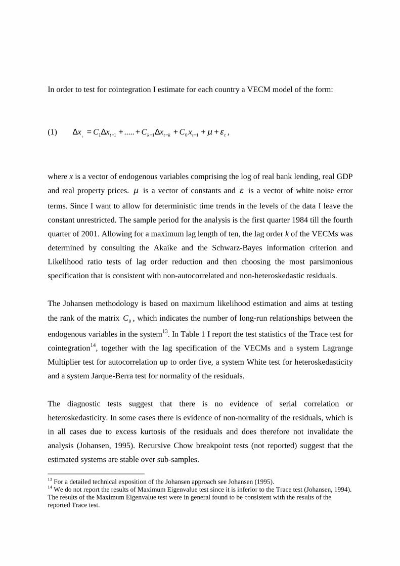
In order to test for cointegration I estimate for each country a VECM model of the form:

(1) ttktkt xCxCxCxt

εµ +++∆++∆=∆ −−−− 10111 ..... ,

where x is a vector of endogenous variables comprising the log of real bank lending, real GDP

and real property prices. µ is a vector of constants and ε is a vector of white noise error

terms. Since I want to allow for deterministic time trends in the levels of the data I leave the

constant unrestricted. The sample period for the analysis is the first quarter 1984 till the fourth

quarter of 2001. Allowing for a maximum lag length of ten, the lag order k of the VECMs was

determined by consulting the Akaike and the Schwarz-Bayes information criterion and

Likelihood ratio tests of lag order reduction and then choosing the most parsimonious

specification that is consistent with non-autocorrelated and non-heteroskedastic residuals.

The Johansen methodology is based on maximum likelihood estimation and aims at testing

the rank of the matrix 0C , which indicates the number of long-run relationships between the

endogenous variables in the system13. In Table 1 I report the test statistics of the Trace test for

cointegration14, together with the lag specification of the VECMs and a system Lagrange

Multiplier test for autocorrelation up to order five, a system White test for heteroskedasticity

and a system Jarque-Berra test for normality of the residuals.

The diagnostic tests suggest that there is no evidence of serial correlation or

heteroskedasticity. In some cases there is evidence of non-normality of the residuals, which is

in all cases due to excess kurtosis of the residuals and does therefore not invalidate the

analysis (Johansen, 1995). Recursive Chow breakpoint tests (not reported) suggest that the

estimated systems are stable over sub-samples.

13 For a detailed technical exposition of the Johansen approach see Johansen (1995).14 We do not report the results of Maximum Eigenvalue test since it is inferior to the Trace test (Johansen, 1994).The results of the Maximum Eigenvalue test were in general found to be consistent with the results of thereported Trace test.

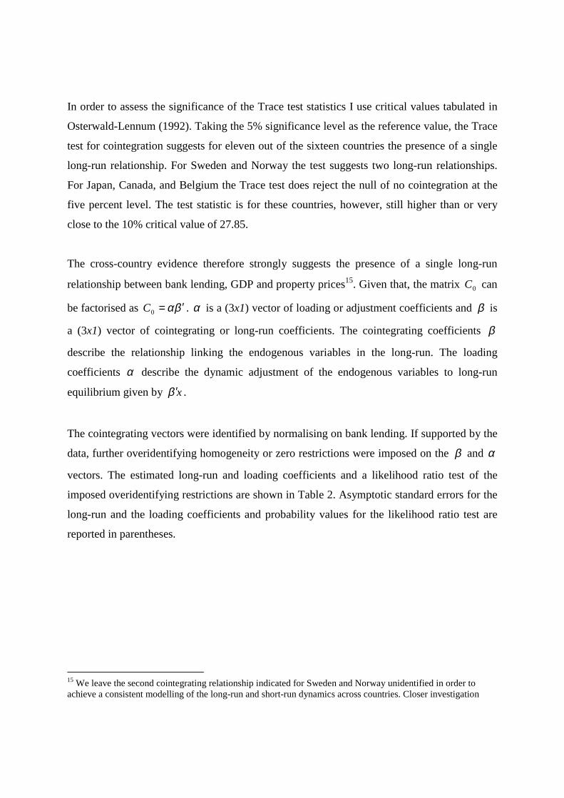
In order to assess the significance of the Trace test statistics I use critical values tabulated in

Osterwald-Lennum (1992). Taking the 5% significance level as the reference value, the Trace

test for cointegration suggests for eleven out of the sixteen countries the presence of a single

long-run relationship. For Sweden and Norway the test suggests two long-run relationships.

For Japan, Canada, and Belgium the Trace test does reject the null of no cointegration at the

five percent level. The test statistic is for these countries, however, still higher than or very

close to the 10% critical value of 27.85.

The cross-country evidence therefore strongly suggests the presence of a single long-run

relationship between bank lending, GDP and property prices15. Given that, the matrix 0C can

be factorised as βα ′=0C . α is a (3x1) vector of loading or adjustment coefficients and β is

a (3x1) vector of cointegrating or long-run coefficients. The cointegrating coefficients β

describe the relationship linking the endogenous variables in the long-run. The loading

coefficients α describe the dynamic adjustment of the endogenous variables to long-run

equilibrium given by xβ ′ .

The cointegrating vectors were identified by normalising on bank lending. If supported by the

data, further overidentifying homogeneity or zero restrictions were imposed on the β and α

vectors. The estimated long-run and loading coefficients and a likelihood ratio test of the

imposed overidentifying restrictions are shown in Table 2. Asymptotic standard errors for the

long-run and the loading coefficients and probability values for the likelihood ratio test are

reported in parentheses.

15 We leave the second cointegrating relationship indicated for Sweden and Norway unidentified in order toachieve a consistent modelling of the long-run and short-run dynamics across countries. Closer investigation

Table 1: Cointegration Test Results

Cointegration Test Diagnostics

0=r 1≤r 2≤r SC H N

USALags = 6

31.72* 9.97 1.78 9.82 234.97 19.72**

JapanLags = 3

27.89 13.6 1.39 4.34 100.96 7.66

GermanyLags = 4

39.29** 13.96 1.57 7.02 142.10 149.50**

FranceLags = 1

30.12* 7.61 0.43 6.98 57.44 4.48

ItalyLags = 10

39.94** 6.70 0.92 7.21 379.12 72.13**

UKLags = 1

30.63* 10.90 2.21 7.16 205.30 15.52*

CanadaLags = 3

27.65 10.30 0.16 8.10 134.96 13.98*

AustraliaLags = 4

31.40* 10.13 2.01 3.26 154.61 12.21

SwedenLags = 8

54.96** 18.17* 0.17 7.47 323.83 29.13**

NorwayLags = 2

66.84** 30.99** 4.29* 9.49 103.70 4.75

FinlandLags = 4

31.48* 12.48 0.01 11.28 162.62 8.07

NetherlandsLags = 8

30.32* 5.44 0.24 7.65 293.58 20.33**

BelgiumLags = 5

29.61 10.39 0.03 2.51 184.53 14.51*

IrelandLags = 9

45.58** 12.26 4.20* 9.62 359.69 32.29**

Hong KongLags = 7

40.19** 7.56 0.11 8.96 283.02 17.04**

SingaporeLags = 4

31.29* 6.10 0.41 7.30 49.48 4.34

Note: The table displays the test statistics of the Johansen trace test for cointegration. The 5%(1%) critical values for the cointegration test are 29.68 (35.65), 15.41 (20.04), 3.76 (6.65) forr=0, r=1, r=2 respectively (Osterwald-Lenum, 1992). SC is a system Lagrange multiplier testfor residual serial correlation up to order 5, H is a system White test for residualheteroskedasticity and N s a system Jarque-Berra test for residual normality. * and **indicates significance of a test statistic at the 5% and 1% level respectively.

suggested that the second cointegrating vector might be a long-run asset pricing relationship linking propertyprices to real GDP.

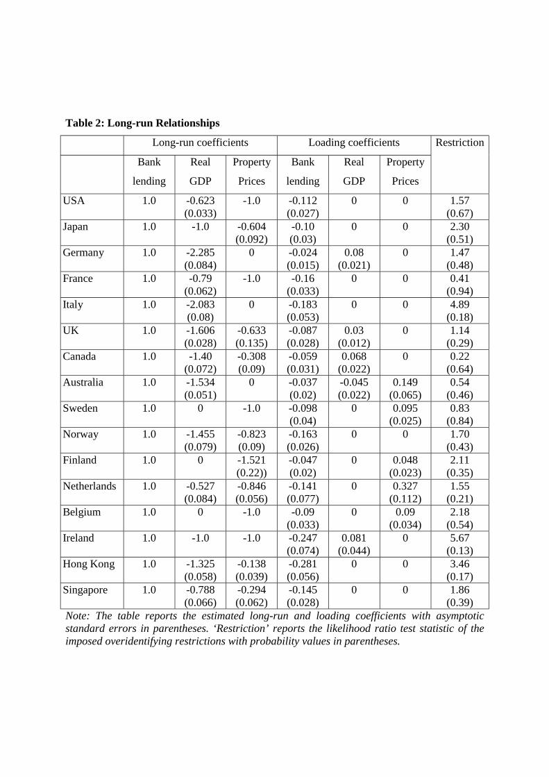
Table 2: Long-run Relationships

Long-run coefficients Loading coefficients

Bank

lending

Real

GDP

Property

Prices

Bank

lending

Real

GDP

Property

Prices

Restriction

USA 1.0 -0.623(0.033)

-1.0 -0.112(0.027)

0 0 1.57(0.67)

Japan 1.0 -1.0 -0.604(0.092)

-0.10(0.03)

0 0 2.30(0.51)

Germany 1.0 -2.285(0.084)

0 -0.024(0.015)

0.08(0.021)

0 1.47(0.48)

France 1.0 -0.79(0.062)

-1.0 -0.16(0.033)

0 0 0.41(0.94)

Italy 1.0 -2.083(0.08)

0 -0.183(0.053)

0 0 4.89(0.18)

UK 1.0 -1.606(0.028)

-0.633(0.135)

-0.087(0.028)

0.03(0.012)

0 1.14(0.29)

Canada 1.0 -1.40(0.072)

-0.308(0.09)

-0.059(0.031)

0.068(0.022)

0 0.22(0.64)

Australia 1.0 -1.534(0.051)

0 -0.037(0.02)

-0.045(0.022)

0.149(0.065)

0.54(0.46)

Sweden 1.0 0 -1.0 -0.098(0.04)

0 0.095(0.025)

0.83(0.84)

Norway 1.0 -1.455(0.079)

-0.823(0.09)

-0.163(0.026)

0 0 1.70(0.43)

Finland 1.0 0 -1.521(0.22))

-0.047(0.02)

0 0.048(0.023)

2.11(0.35)

Netherlands 1.0 -0.527(0.084)

-0.846(0.056)

-0.141(0.077)

0 0.327(0.112)

1.55(0.21)

Belgium 1.0 0 -1.0 -0.09(0.033)

0 0.09(0.034)

2.18(0.54)

Ireland 1.0 -1.0 -1.0 -0.247(0.074)

0.081(0.044)

0 5.67(0.13)

Hong Kong 1.0 -1.325(0.058)

-0.138(0.039)

-0.281(0.056)

0 0 3.46(0.17)

Singapore 1.0 -0.788(0.066)

-0.294(0.062)

-0.145(0.028)

0 0 1.86(0.39)

Note: The table reports the estimated long-run and loading coefficients with asymptoticstandard errors in parentheses. ‘Restriction’ reports the likelihood ratio test statistic of theimposed overidentifying restrictions with probability values in parentheses.

The results suggest that in most countries real GDP and real property prices both enter the

cointegrating vector. The long-run coefficient of real GDP is not significantly different from

zero in Sweden, Finland and Belgium, while the restriction that bank lending is homogenous

to real GDP is not rejected for Japan and Ireland. The long-run GDP elasticity is found to be

significantly larger than one in Germany, Italy, the UK, Canada, Australia, Norway and Hong

Kong and significantly smaller than one in the USA, France, the Netherlands and Singapore.

A zero restriction on the long-run property price coefficient is not rejected for Germany, Italy

and Australia, while long-run homogeneity of bank lending to property prices is not rejected

for the USA, France, Sweden, Belgium and Ireland. In all other countries, the long-run

property price coefficient is significantly smaller than one except for Finland, which is the

only case where it is significantly larger than one.

The loading coefficient in the bank lending equation is significantly smaller than zero in every

country. The loading coefficient in the GDP equation is significant only in Germany, the UK,

Canada, Australia and Ireland, that in the property price equation only in Australia, Sweden,

Finland, the Netherlands and Belgium. This finding suggests that it is bank lending rather than

real GDP or property prices that takes the system back to long-run equilibrium.

5. Dynamic Interaction

In this section I estimate, based on the VECMs estimated in the previous section, error-

correction models for credit growth and the change in property prices. The error-correction

models are of the form:

(2) tl

ltl

n

kktk

n

jjtj

n

iititt rpylCIl εγγγγγ ∑ ++∑ ∆+∑ ∆+∑ ∆+=∆

=−

=−

=−

=−−

5

14

13

02

0110

(3) tl

ltl

n

kktk

n

jjtj

n

iititt rlypCIp υλλλλλ ∑ ++∑ ∆+∑ ∆+∑ ∆+=∆

=−

=−

=−

=−−

5

14

13

02

0110 ,

where l∆ is real lending growth, y∆ is real GDP growth, p∆ is the change in real property

prices and r is the short-term real interest rate. CI is the cointegrating vector linking the levels

of real bank lending, real GDP and real property prices reported in Table 2. In each equation I

chose the lag order selected for the VECMs in the previous section, which are reported in

Table 1, as the maximum lag length n considered for the change in real lending, real GDP

growth and the change in real property prices. For the short-term real interest rate I consider

up to five lags. The error-correction models were then estimated by applying a general-to-

specific modelling strategy eliminating sequentially the least significant lag until all retained

lags were significant at least at the 10% level. The full results are reported in Appendix-

Tables 1 and 2. In Table 3 and 4 I report the error-correction coefficient and the sum of the

coefficients of the retained lags of each variable with t-statistics in parentheses.

Table 3 reports the results for the error-correction model for credit growth. Coefficients,

which are significant at least at the 10% level, are in bold. A zero indicates that no single lag

was found to be significant so that all lags of the variable were eliminated from the model.

The error-correction coefficient is significant in every country, providing strong cross country

evidence of long-run causality going from economic activity and property prices to bank

lending. There is also evidence of short-run causality going from GDP and property prices to

bank lending. In eight countries I find a significant effect of lagged real GDP growth on credit

growth. In six countries the effect is significantly positive, while it is significantly negative in

Japan and Hong Kong. In thirteen countries I find evidence of short-run causality going from

property prices to lending. The overall effect is insignificant in four countries and

significantly positive in nine. A significantly negative real interest rate effect is found in only

four countries.

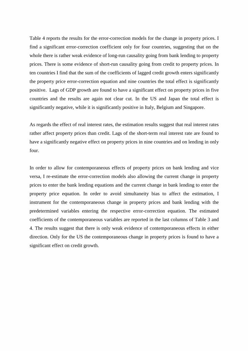
Table 4 reports the results for the error-correction models for the change in property prices. I

find a significant error-correction coefficient only for four countries, suggesting that on the

whole there is rather weak evidence of long-run causality going from bank lending to property

prices. There is some evidence of short-run causality going from credit to property prices. In

ten countries I find that the sum of the coefficients of lagged credit growth enters significantly

the property price error-correction equation and nine countries the total effect is significantly

positive. Lags of GDP growth are found to have a significant effect on property prices in five

countries and the results are again not clear cut. In the US and Japan the total effect is

significantly negative, while it is significantly positive in Italy, Belgium and Singapore.

As regards the effect of real interest rates, the estimation results suggest that real interest rates

rather affect property prices than credit. Lags of the short-term real interest rate are found to

have a significantly negative effect on property prices in nine countries and on lending in only

four.

In order to allow for contemporaneous effects of property prices on bank lending and vice

versa, I re-estimate the error-correction models also allowing the current change in property

prices to enter the bank lending equations and the current change in bank lending to enter the

property price equation. In order to avoid simultaneity bias to affect the estimation, I

instrument for the contemporaneous change in property prices and bank lending with the

predetermined variables entering the respective error-correction equation. The estimated

coefficients of the contemporaneous variables are reported in the last columns of Table 3 and

4. The results suggest that there is only weak evidence of contemporaneous effects in either

direction. Only for the US the contemporaneous change in property prices is found to have a

significant effect on credit growth.

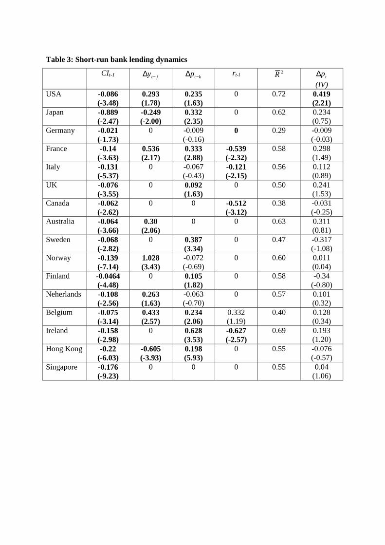
Table 3: Short-run bank lending dynamics

CIt-1 jty −∆ ktp −∆ rt-l 2R tp∆(IV)

USA -0.086(-3.48)

0.293(1.78)

0.235(1.63)

0 0.72 0.419(2.21)

Japan -0.889(-2.47)

-0.249(-2.00)

0.332(2.35)

0 0.62 0.234(0.75)

Germany -0.021(-1.73)

0 -0.009(-0.16)

0 0.29 -0.009(-0.03)

France -0.14(-3.63)

0.536(2.17)

0.333(2.88)

-0.539(-2.32)

0.58 0.298(1.49)

Italy -0.131(-5.37)

0 -0.067(-0.43)

-0.121(-2.15)

0.56 0.112(0.89)

UK -0.076(-3.55)

0 0.092(1.63)

0 0.50 0.241(1.53)

Canada -0.062(-2.62)

0 0 -0.512(-3.12)

0.38 -0.031(-0.25)

Australia -0.064(-3.66)

0.30(2.06)

0 0 0.63 0.311(0.81)

Sweden -0.068(-2.82)

0 0.387(3.34)

0 0.47 -0.317(-1.08)

Norway -0.139(-7.14)

1.028(3.43)

-0.072(-0.69)

0 0.60 0.011(0.04)

Finland -0.0464(-4.48)

0 0.105(1.82)

0 0.58 -0.34(-0.80)

Neherlands -0.108(-2.56)

0.263(1.63)

-0.063(-0.70)

0 0.57 0.101(0.32)

Belgium -0.075(-3.14)

0.433(2.57)

0.234(2.06)

0.332(1.19)

0.40 0.128(0.34)

Ireland -0.158(-2.98)

0 0.628(3.53)

-0.627(-2.57)

0.69 0.193(1.20)

Hong Kong -0.22(-6.03)

-0.605(-3.93)

0.198(5.93)

0 0.55 -0.076(-0.57)

Singapore -0.176(-9.23)

0 0 0 0.55 0.04(1.06)

Table 4: Short-run property price dynamics

CIt-1 jty −∆ ktl −∆ rt-l 2R tp∆(IV)

USA 0 -0.283(-2.23)

0.213(2.77)

0 0.59 0.092(0.68)

Japan 0 -0.18(-2.03)

0.321(4.87)

-0.417(-2.96)

0.78 0.077(0.55)

Germany 0 0 0 -0.728(-2.51)

0.69 -0.214(-0.69)

France 0 0 0 -0.294(-1.85)

0.74 0.004(0.03)

Italy 0 1.494(3.87)

0.382(2.53)

0 0.73 0.049(0.27)

UK 0 0 0.477(2.72)

0 0.30 -0.171(-0.31)

Canada 0 0.055(0.12)

0 -1.051(-2.09)

0.13 0.745(1.28)

Australia 0.172(3.26)

0 0.737(3.05)

-0.79(-2.74)

0.31 0.119(1.43

Sweden 0 0 0 -0.425(-2.69)

0.66 -0.037(-0.27)

Norway 0 0 0.3586(2.87)

-0.833(-1.62)

0.37 0.064(0.25)

Finland 0.049(4.40)

0 0.591(3.89)

-0.781(-2.43)

0.73 0.732(0.44)

Netherlands 0.13(2.22)

0 0.351(2.24)

0 0.42 0.241 (0.73)

Belgium 0.095(4.05)

0.225(2.04)

0.236(2.38)

0 0.24 0.213(1.50)

Ireland 0 0 -0.042(-0.27

0 0.36 0.174(0.95)

Hong Kong 0 0 0 0 0.43 0.165(0.39)

Singapore 0 0.649(2.44)

0 -2.85(-2.46)

0.51 -0.357(-0.94)

5. Conclusions

Over the last two decades, bank lending has been closely correlated with property prices in

both industrialised and developing countries. Theory suggests that property prices may affect

credit via various wealth effects, while credit may affect property prices via various liquidity

effects. From previous empirical studies it is not clear which effect dominates, since the

focus is usually on either effect but not on both. In this study I analyse the direction of

causality between bank lending and property prices in 16 industrialised countries over the

last two decades.

Cointegration analysis suggests that in all countries there is evidence of a long-run

relationship between bank lending, economic activity and property prices, with long-run

causality going from property prices and economic activity to bank lending. This finding

suggests that property price cycles, reflecting changing beliefs about future economic

prospects, drive credit cycles, rather than excessive bank lending, in the wake of financial

liberalisation, being the cause of property price bubbles.

The results of estimating error-correction equations for credit growth and the change in

property prices suggest that there is evidence of short-run causality going in both directions.

This implies that a mutually re-enforcing element in past boom bust cycles in credit and

property markets cannot be ruled out.

References

Ando, A. and F. Modigliani (1963). The ‘Life Cycle’ Hypothesis of Saving: Aggregate

Implications and Tests. American Economic Review, 53, 55-84.

Bernanke, B. and M. Gertler (1989). Agency Costs, Collateral and Business Fluctuations.

American Economic Review, 79, 14-31.

Bernanke, B., M. Gertler and S. Gilchrist (1998). The Financial Accelerator in a Quantitative

Business Cycle Framework. NBER Working Paper No. 6455.

BIS (1999). The Monetary and Regulatory Implications of Changes in the Banking Industry.

BIS Conference Papers No.7.

BIS (2001), 71st Annual Report.

Borio, C. and W. Fritz (1995). The Response of Short-Term Bank Lending Rates to policy

Rates: A Cross-Country Perspective. BIS Working Paper No. 27.

Borio, C., N. Kennedy and S. Prowse (1994). Exploring Aggregate Asset Price Fluctuations

across Countries: Measurement, Determinants and Monetary Policy Implications.

Bank for International Settlements. BIS Working Paper No. 40.

Deaton, A. (1992). Understanding Consumption. Oxford University Press.

Dickey, D. and W. Fuller (1981). Likelihood Ratio Statistics for Autoregressive Time Series

with a Unit Root. Econometrica, 60, 423-433.

Drees, B. and C. Pazarbasioglu (1998). The Nordic Banking Crises. Pitfalls in Financial

Liberalization? IMF Occasional Paper No. 161.

Fisher, I. (1933). The Debt-Deflation Theory of Great Depressions. Econometrica, 1, 337-57.

Goodhart, C. (1995). Price Stability and Financial Fragility. In: K. Sawamoto, Z. Nakajima

and H. Taguchi (Eds.). Financial Stability in a Changing Environment. St. Martin’s

Press.

Hofmann, B. (2001). The Pass-Through of Money Market Rates to Loan Rates in the Euro-

Area. Mimeo, ZEI, University of Bonn.

Hofmann, B. and P. Mizen (2001). Base Rate Pass-Through in UK Banks’ and Building

Societies’ Retail Rates. Mimeo, Bank of England.

Hoshi, T. and A. Kashyap (1999). The Japanese Banking Crisis: Where Did it Come from and

How Will it End? NBER Working Paper No. 7250.

IMF (2000). World Economic Outlook, May 2000.

Johansen, S. (1988). Statistical Analysis of Cointegration Vectors. Journal of Economic

Dynamics and Control, 12, 231-54.

Johansen, S. (1994). The Role of the Constant and Linear Terms in Cointegration Analysis of

Non-Stationary Variables.. Econometric Reviews, 13, 205-229.

Johansen, S. (1995). Likelihood-Based Inference in Cointegrated Vector Autoregressive

Models. Oxford University Press.

Keynes, J. (1931). The Consequences for the Banks of the Collapse in Money Values. In:

Essays in Persuasion, Macmillan.

Kindleberger, C. (1978). Manias, Panics and Crashes: A History of Financial Crises. In: C.

Kindleberger and J. Laffarge (Eds.) Financial Crises: Theory, History and Policy,

Cambridge University Press.

Kiyotaki, N. and J. Moore (1997). Credit Cycles. Journal of Political Economy, 105, 211-248.

Minsky, H. (1982), ‘Can ‘’It’’ happen again?’, Essays on Instability and Finance, M.E.Sharpe

Muellbauer, J. (1994). The Assessment: Consumer Expenditure. Oxford Review of Economic

Policy, 10, 1-41.

OECD (2000), Economic Outlook 68, December 2000.

Osterwald-Lenum, M. (1992). A Note with Quantiles of the Asymptotic Distribution of the

Maximum Likelihood Cointegration Rank Test Statistics, Oxford Bulletin of

Economics and Statistics, 54, 461-472.

Phillips, P. and P. Perron (1988). Testing for a Unit Root in Time Series Regression.

Biometrika, 75, 335-346.