Working Paper 9604

BANK DEPOSIT RATE CLUSTERING:

THEORY AND EMPIRICAL EVIDENCE

by Charles Kahn, George Pennacchi,and Ben Sopranzetti

Charles Kahn is a professor of finance at the Universityof Illinois; George Pennacchi is an associate professor offinance at the University of Illinois and a research associateat the Federal Reserve Bank of Cleveland; and BenSopranzetti is an assistant professor of finance at SeattleUniversity. The authors are very grateful to DouglasEvanoff, Allen Berger, Richard Rosen, and Arlene Sopranzettifor help with the empirical work of this paper. Useful commentswere provided by seminar participants at Indiana University,Seattle University, the University of Illinois, and the 1996Winter Econometric Society Meetings. Correspondence maybe sent to George Pennacchi, Department of Finance, Universityof Illinois, 1407 West Gregory Drive, Urbana, Ill. 61801.Phone: (217) 244-0952. FAX: (217) 244-3102. Email:gpennacc@uiuc.edu.

Working papers of the Federal Reserve Bank of Clevelandare preliminary materials circulated to stimulate discussion andcritical comment. The views contained herein are those ofthe authors and not necessarily those of the Federal ReserveBank of Cleveland or of the Board of Governors of theFederal Reserve System.

Working papers are now available electronically through theCleveland Fed�s home page on the World Wide Web:http://www.clev.frb.org.

July 1996

Abstract

The market prices of stocks and other assets tend to cluster on round fractions. A similar clustering is foundin the interest rates paid on retail bank deposits. However, the theoretical rationales given for asset-priceclustering are incompatible with the clustering of retail deposit rates. This paper proposes a theory based ondepositors� limited recall. It shows that when banks exploit this phenomenon, deposit rates will tend to beset at round fractions and will be relatively �sticky� at these levels. The implications of this theoreticalmodel are tested using money market deposit account and retail certificate of deposit interest-rate data from asample of more than 500 banks.

2

I. Introduction

A central issue in economic theory is the determination of market prices, but standard

price theory cannot explain several common pricing conventions. These conventions are difficult

to rationalize because they depend on the pricing system�s unit of account. For example, in many

financial markets, asset prices tend to cluster around �even� fractions of currency units. Several

papers, including Osborne (1962), Nierderhoffer (1965), Harris (1991), and Christie and Schultz

(1994), document that integer-dollar stock prices are more common than half-dollar stock prices,

which are more common than quarter-dollar prices, which are more common than eighth-dollar

prices. This phenomenon occurs for both stock quotes and transaction prices, and is persistent

through time and across different stocks and stock markets. Ball, Torous, and Tschoegl (1985)

find a similar clustering in the London gold market�s fixing (auction) prices, as do Goodhart and

Curcio (1990) in foreign exchange rates. Colwell, Rushing, and Young (1994) show that

residential real estate prices tend to cluster on whole thousands and five-hundreds.

Explicit rules can require that prices cluster at particular fractions, an example being

stock-exchange regulations that allow price quotes at �tick� sizes no smaller than an eighth of a

dollar. More interesting are cases where clustering is not mandated, but results from an implicit

agreement (custom) among traders. Two main theoretical explanations for such agreements have

been proposed in the literature. First, as discussed by Harris (1991) and Ball, Torous, and

Tschoegl (1985), and as modeled by Brown, Laux, and Schachter (1991), the custom of clustering

on discrete price sets can be a mechanism for reducing the cost of negotiating transactions. By

limiting bids and offers to a given set of prices, negotiations can be consummated more rapidly,

since frivolous revisions of quotes at minute increments cannot be made. Limiting quotes to

rounded prices can also make recording prices easier, thereby decreasing errors from traders

believing that they have traded at different prices. This implicit agreement can be self-enforcing if

3

professional traders deal with each other on a repeated basis, since noncooperation by an

individual could lead to his exclusion from future trading.1 As an alternative to this negotiation-

cost hypothesis, Christie and Schultz (1994) and Christie, Harris, and Schultz (1994) propose a

second rationale for price clustering. In their view, an agreement to limit price quotes to round

fractions may be motivated by the desire to maintain noncompetitive bid-ask spreads. They

present evidence that dealers in NASDAQ stocks avoided odd-eighths price quotes in order to

maintain quarter-point bid-ask spreads.

If clustering around even fractions is a device for reducing negotiation costs or

maintaining noncompetitive bid-ask spreads, one would expect that even-fraction clustering would

not be pervasive in markets where prices are not negotiated and traders do not make a two-way

market (quote both bid and ask prices). Indeed, this appears to be the case in many retail markets

where sales to consumers are typically not negotiated and almost always occur at the sellers�

quotes. In these non-negotiated, one-way retail markets, the tendency is to quote �odd� prices,

where an odd price (e.g., $3.99) is defined as one whose right-most digits are just below a whole

or �even� price (e.g., $4.00). The unusually high occurrence of odd prices in retail markets, such

as department, discount, and grocery stores, is well documented. For example, in an analysis of

scanner data, Wisniewski and Blattberg (1983) found that over 80 percent of prices quoted by a

major supermarket chain ended with the digit 9. Friedman (1967) and Kashyap (1995) also

document this odd-pricing phenomenon.

The absence of negotiations and bid-ask spreads might explain why retail prices are

generally not rounded, but the unusually high frequency of odd-pricing in these markets requires

its own explanation. The convention of odd-pricing in non-negotiated retail markets might be

1 Casual observation is consistent with repeated dealings being an important factor in supporting theseimplicit agreements. In situations where successive dealings are unlikely, as in the auctioning of uniquegoods, explicit rules that restrict prices are often enforced. For example, English auctions typically require

that new bids exceed a standing bid by a minimum price increment.

4

linked to the different incentives and lack of information possessed by retail consumers compared

to wholesale market traders. Transactions in wholesale markets are typically large, so that minute

percentage price differences can have major consequences. Negotiating to obtain the best

possible price is a paramount concern for professional traders. In contrast, retail consumers,

whose transactions are smaller, may have less incentive to analyze which seller is offering the best

price. Unlike wholesale traders, who typically have instant access to price quotes from many

other traders, retail consumers usually obtain quotes from sellers of a given product at different

points in time. They receive price information, either through advertisements or when shopping, in

a sequential manner, but it may not be worth their time and effort to carefully record different

sellers� prices. Hence, retail consumers� ability to recall prior price quotes will affect their

current buying decisions.

Importantly, experimental tests performed by Schindler and Wiman (1989) find that

individuals tend to recall odd-ending prices less accurately than even-ending prices, and that

expressing a price as odd-ending increases the likelihood that it will be underestimated when

recalled. A biological explanation for this downward bias in recalling odd-ending prices is offered

by Brenner and Brenner (1982). They propose a theory of fixed storage capacity which assumes

that the extra decision of rounding the initially observed number is costly, so that the cheapest

�transfer mechanism� involves simply storing the first digit. Hence, if a price�s right-most digits

are not stored in memory, odd-ending prices will tend to be underestimated. If firms recognize

consumers� downward bias in recalling odd-ending prices, they may significantly increase the

demand for their products by making odd-ending price quotes rather than slightly higher even-

ending ones. Even-ending quotes will then represent �pricing points� where product demand

experiences a discrete decline. Blinder (1991) reports some empirical support for this notion.

5

Based on interviews with firm managers, he finds that a majority were reluctant to cross the

�psychological barrier� of raising prices from an odd-ending quote to an even-ending one.

Not all firms that market retail products or services quote prices, however. For example,

financial institutions customarily quote interest rates (yields), rather than prices, for many of their

fixed-income investments. An intriguing question is whether the retail customers of these financial

firms suffer from a similar downward bias when recalling odd-ending yields and, if so, whether

these firms attempt to exploit this behavioral phenomenon. Financial institutions would take

advantage of this customer behavior by quoting retail loan rates with odd-ending yields (so that

they would be underestimated when recalled), but, in contrast, by quoting retail deposit rates with

even-ending yields (so that they would not be underestimated when recalled). There is some

anecdotal evidence that banks may in fact engage in this practice. During 1986-87, Davis,

Korobow, and Wenninger (1987) conducted a series of interviews with senior commercial and

savings bank officers in the New York City area. In their article (page 8), they report:

One banker offered the explanation that as market rates have declined, bankshave been reluctant to breach successive single digit �floors� (such as an even6.00 percent) and have been particularly slow to cut MMDA (Money MarketDeposit Account) rates below the old ceiling rate on regular savings depositseven though such cuts might be justified on cost of money grounds. Such a lineof argument would suggest that the bankers believe that at least at some criticalpoints, the rate elasticity of demand for MMDAs may be fairly high, so that theyfear losing market share by cutting rates at such points.

While there is an extensive literature analyzing how banks set their retail deposit rates, the

possibility that they might exploit the limited recall of their depositors has not been investigated.2

The goal of this paper is to consider such a possibility. We analyze a banking firm�s optimal

deposit-rate-setting behavior when some consumers have limited recall but others have full recall.

In section II, we present a model in which the demand for bank deposits by

2 Some recent research on banks� deposit-rate-setting behavior includes Diebold and Sharpe (1990), Hannanand Berger (1991), Neumark and Sharpe (1992), and Rosen (1995).

6

full-recall consumers depends on the bank�s actual interest rate (e.g., 3.29 percent), whereas the

demand by limited-recall consumers depends on the integer floor of the actual rate (e.g., 3.00

percent). In this environment, we solve for a bank�s profit-maximizing deposit rate as a function

of its opportunity cost of funds (wholesale-market funding rate) and the proportion of limited-

recall consumers in its market.

We find that the bank�s optimal deposit rate is set either at a whole integer or at an

interior point that satisfies a particular first-order condition. The likelihood of rates being set to

an integer increases along with the proportion of limited-recall consumers and the wholesale cost

of funds. As a consequence, our theory predicts that retail deposit rates will tend to cluster on

integer digits, but for an entirely different reason than those given for price clustering in

negotiated, two-way financial markets. We also show that for a given cost-of-funds shock, the

bank�s deposit rate is less likely to change when it is currently at an integer value than when it is

not. Thus, deposit rates tend to be �sticky� at integer values. In addition, although deposit rates

become stickier as the bank�s cost of funds increases, when changes do occur, they will tend to

move the deposit rate from one integer to another.

One of the attractive features of studying the pricing behavior of a banking firm, as

opposed to a nonfinancial firm, is that a relatively accurate measure of changes in �input� or

�production� costs is available. Changes in a wholesale funding rate, such as the London

Interbank Offer Rate (LIBOR), give a fairly precise measure of changes in a bank�s input or

opportunity costs. This allows for relatively powerful empirical tests of our model�s predictions.

In section III, we test the model�s implications using monthly money market deposit account

(MMDA) and retail certificate of deposit (CD) rates for more than 500 banks over a 10-1/2-year

period. Our empirical tests strongly support the clustering and sticky-integer implications of the

model.

7

II. A Model of Deposit Pricing with Limited-Recall Investors

Consider the following demand relationship for a particular bank�s retail deposits. Let

D(t) denote investors� date t desired holdings of a given type of retail deposit:

D t D r t r t x td

( ) ( ( ), ( ), ( ))= ,

(1)

where rd(t) is the date t percentage interest rate that the bank offers on this deposit, r(t) is the date

t market rate on wholesale funds of the same maturity as the retail deposit, and x(t) is a vector of

other variables affecting deposit demand. Deposit demand is monotonically increasing in rd .

The relationship in (1) is assumed to be the demand for deposit balances from full-recall

investors, hereafter referred to as �sophisticated� investors. For limited-recall investors, hereafter

referred to as �naive� investors, the functional form is the same, but instead of the argument rd,

naive investors base their demands on a noisy, downward-biased measure of the actual deposit

rate. In the spirit of Schindler and Wiman (1989) and Brenner and Brenner (1982), we assume that

naive investors� demands depend on a truncated version of rd, so that the interest rate they

observe is the true deposit rate reported only as an integer-valued percentage rate. In other words,

if the true offered depository rate is 5.30 percent, naive investors will observe 5.00 percent.

We will denote by [ ]r − the truncation, or integer floor, of the real variable r. Similarly,

let [ ]r + denote the integer ceiling of the variable r. Thus, the demand curve for naive investors

can be represented by

D r t r t x td

( ( ),[ ( )] , ( ))− .

(2)

Let k be the proportion of potential bank customers who are naive, so that 1-k is the proportion

who are sophisticated. Also, let c be the bank�s non-interest expense per dollar of deposit. Then,

the following function represents the bank�s profits at date t from issuing retail deposits:

8

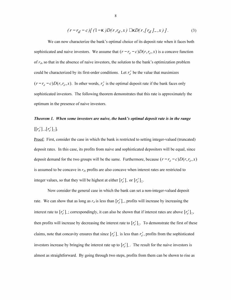
( )[ ( ) ( , , ) ( ,[ ] , ) ]r r c D r r x D r r xd d d− − − + −1 κ κ . (3)

We can now characterize the bank�s optimal choice of its deposit rate when it faces both

sophisticated and naive investors. We assume that ( ) ( , , )r r c D r r xd d

− − is a concave function

of rd, so that in the absence of naive investors, the solution to the bank�s optimization problem

could be characterized by its first-order conditions. Let rd

s be the value that maximizes

( ) ( , , )r r c D r r xd d

− − . In other words, rd

s is the optimal deposit rate if the bank faces only

sophisticated investors. The following theorem demonstrates that this rate is approximately the

optimum in the presence of naive investors.

Theorem 1. When some investors are naive, the bank�s optimal deposit rate is in the range

[[ ] ,[ ] ]r rd

s

d

s

− + .

Proof: First, consider the case in which the bank is restricted to setting integer-valued (truncated)

deposit rates. In this case, its profits from naive and sophisticated depositors will be equal, since

deposit demand for the two groups will be the same. Furthermore, because ( ) ( , , )r r c D r r xd d

− −

is assumed to be concave in rd, profits are also concave when interest rates are restricted to

integer values, so that they will be highest at either [ ]rd

s

− or [ ]rd

s

+ .

Now consider the general case in which the bank can set a non-integer-valued deposit

rate. We can show that as long as rd is less than [ ]rd

s

− , profits will increase by increasing the

interest rate to [ ]rd

s

− ; correspondingly, it can also be shown that if interest rates are above [ ]rd

s

+ ,

then profits will increase by decreasing the interest rate to [ ]rd

s

+ . To demonstrate the first of these

claims, note that concavity ensures that since [ ]rd

s

− is less than rd

s, profits from the sophisticated

investors increase by bringing the interest rate up to [ ]rd

s

− . The result for the naive investors is

almost as straightforward. By going through two steps, profits from them can be shown to rise as

9

well. From any initial interest rate rd, bring interest rates down to [ ]rd − . This increases profits

from naive investors. Next, increase profits further by moving from [ ]rd − to [ ]r

d

s

− . QED

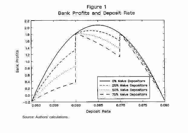
The effect of including naive investors is illustrated in figure 1, which shows a bank�s

profit as a function of its deposit rate for various proportions of naive investors in the population.3

When all investors are sophisticated (k=0), as indicated by the solid line, profits are a smooth

function of the offered interest rates, and the profit-maximizing rate is rd

s = 6.5 percent. In

contrast, when three-quarters of the investors are naive (k=.75), as indicated by the long dashed

line, bank profits increase dramatically as the interest rate moves from, say, 5.9 percent to 6.0

percent, as this brings in a large number of depositors. From that point, small increases in interest

rates decrease profits, until the next breakpoint is achieved. Thus, the profitable thing to do when

most investors are naive is to set the deposit rate at a breakpoint.

When many, but not all, investors are sophisticated, it may be optimal to choose an

interior deposit rate, although this rate will not be the same as the optimal rate that would be set

when all investors are sophisticated. Figure 1 gives an example of this for the case in which naive

investors make up one-quarter (k=.25) of all depositors. As indicated by the short dashed line,

the profit-maximizing interest rate is at the interior rate of 6.34375 percent.

Theorem 2. When some investors are naive, the bank�s profit-maximizing deposit rate is

either one of the endpoints of the interval described in Theorem 1, or a point in the interior of

this interval that satisfies the following first-order condition:

3 The profit function in figure 1 assumes that c = .005 and D = a0 + a1r + a2rd , where a0=0, a1 = -6,000, and

a2=10,000. This implies that in the absence of naive investors, the profit-maximizing deposit rate is rd

s =

.5[(1- a1/a2)r - c - a0/a2] = .8r - .0025. Assuming a market interest rate of r = 8.4375 percent gives rd

s = 6.5

percent. These parametric assumptions are close to the parameter estimates for MMDAs found in Hutchisonand Pennacchi (1996).

10

r r cD r D r

D r

r

d

d d

d

d

− − = − +

−

−** *

*

*

( ) ( ) ([ ] )

( )( )

1

1

κ κ

κ ∂∂

.

(4)

Roughly speaking, this first-order condition says the following: The optimal deposit rate

is determined by balancing the benefits of increasing the interest rate spread with the cost of losing

deposit market share. The more naive depositors there are, the lower the cost to market share of a

small decrease in the deposit rate. Thus, as long as the choice is interior to the interval, the

deposit rate decreases with increases in the proportion of naive individuals. Eventually, of course,

the number of naive investors becomes great enough that the optimum is a breakpoint -- the

solution jumps to that breakpoint (whole-digit interest rate) and remains there for further increases

in the proportion of naive individuals. The jump may be up or down. In figure 1, we have chosen

a borderline example, so that profits are the same for a jump in either direction.

This theorem gives us a direct means for calculating the optimum. We begin by taking

the optimum in the absence of naive individuals and use it to find the boundary points. We then

compare profits at those points with profits at the value where the first-order condition is satisfied.

Figure 2 plots the optimal deposit rate as a function of the bank�s wholesale market rate, r, for a

given proportion (k=50 percent) of naive individuals in the population.4 Notice that when the

wholesale market rate is low, the optimal deposit rate will be a relatively smooth function of the

market rate. However, as the market rate increases, the function becomes discontinuous, jumping

from one breakpoint to another. Intuitively, when the market rate is fairly low, the incremental

profit from sophisticated depositors� increased demand is large enough to outweigh the marginal

cost of raising the quoted deposit rate. Of course, the opposite is true when the market rate is

relatively high.

4 Figure 2 makes the same demand and non-interest cost assumptions made in figure 1. See footnote 3.

11

Figure 2 illustrates that as the wholesale market rate increases, the likelihood of the bank

setting its retail deposit rate at a breakpoint should also rise. In addition, once the quoted interest

rate is at a breakpoint, the likelihood of the bank changing its deposit rate decreases for any given

change in the market rate. In other words, deposit rates are stickier when they are currently at an

integer value. Figure 2 also demonstrates that although the bank�s propensity to change its

deposit rate decreases with an increase in market rates, when it does make a change, the change

will, ceteris paribus, tend to be greater in magnitude.

III. Empirical Evidence

III.A Data Description and Preliminary Analysis

To test the implications of the model presented in the previous section, we obtained data

on bank deposit rates from the Federal Reserve System�s Survey of Selected Deposits and Other

Accounts. This data set contains monthly retail deposit rates paid by over 500 banks during the

week ending on the last Wednesday of each month. Our sample period extends from November

1983 to May 1994 and contains 42,202 observations of rates paid on MMDAs, 49,137

observations on three-month CDs (CD3s), 50,340 observations on six-month CDs (CD6s), and

49,909 observations on 12-month CDs (CD12s). Although the CD rates in this survey are for

small-denomination (< $100,000) retail CDs, investors� balances held in CDs are generally larger

than those in MMDAs. Also, the potential investor market for CDs is often greater than for

MMDAs. The relevant market for MMDAs is generally limited to the bank�s local depositor

market, whereas CDs may be marketed to investors nationwide through CD brokers.5 An

implication of these differences is that the proportion of naive investors should be relatively

5 Berger and Hannan (1989) find significantly lower rates paid on MMDAs, CD3s, and CD6s by banks inmore concentrated local markets, although the link was strongest for MMDAs. No such relationship wasfound for CD12s.

12

greater for MMDAs than for CDs. Thus, one would expect the effects of limited recall by naive

investors to be more clearly displayed in MMDAs than in CDs.

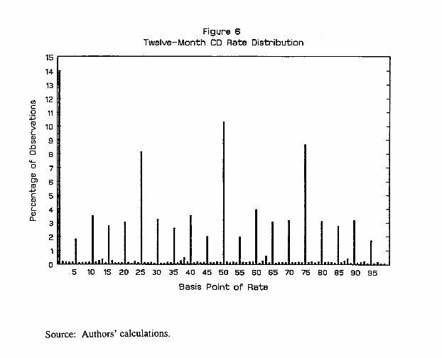
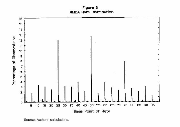
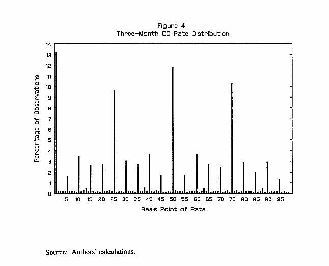
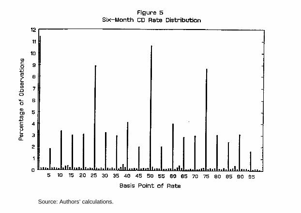
Our theoretical model implies that deposit rates set at or slightly above whole digits

should be more common than rates set just below whole digits. In figures 3 to 6, we present the

frequency distributions of our sample of observations. These histograms show the percentage of

observations at each basis point from 0 to 99, where, for example, 0 refers to a whole-integer

percentage deposit rate and 50 refers to a deposit rate set at half a percent. The figures for both

MMDAs and CDs show that the single most common rate is one set at a whole digit: 15.8 percent

of MMDA, 13.4 percent of CD3, 11.6 percent of CD6, and 14.2 percent of CD12 observations.

In addition, there are �spikes� in the frequency distribution at the half-, quarter-, and three-quarter-

digit levels, and, to a lesser extent, at every five basis points. For example, 48.5 percent of

MMDA, 45.8 percent of CD3, 40.7 percent of CD6, and 41.9 percent of CD12 observations are

rates set at either the whole, half, quarter, or three-quarter digit.

The inordinate frequency of deposit rates at multiples of quarter digits suggests that an

extension of our basic model of depositor recall could consider secondary pricing points at half,

quarter, and three-quarter digits in addition to the primary pricing point of the whole digit. The

data appear consistent with banks� exploiting naive investors� limited recall, where recall is

greatest at the whole digit, followed by recall at the half, quarter, and three-quarter digits. To

capture this phenomenon, our model could be extended to allow for three categories of depositors:

sophisticated full-recall depositors; naive depositors whose recall is limited to the quarter digit;

and naive depositors whose recall is limited to the integer digit.

The existence of secondary pricing points at quarter digits might seem at odds with the

notion that recall is inversely related to the number of decimal places held in memory. For

example, why should 6.5 percent be easier to recall than 6.4 percent? Moreover, it would seem to

13

be a contradiction to think that 6.25 percent or 6.75 percent could be remembered more accurately

and with less downward bias than 6.3 percent or 6.7 percent, as the latter rates require fewer

decimal places to be stored than the former. A resolution of this incongruity is that recall may not

be a simple function of decimal places. Investors may have greater recall of 6.25 percent relative

to 6.2 percent because the former is �stored� as 6 and a �quarter,� not as 6 and .25. While we

know of no direct empirical evidence for this, it is not unreasonable that investors� recollection of

�half,� �quarter,� or �three-quarter� could be more precise than a decimal place such as .1, .2, .3,

.4, .6, .7, .8, or .9. The memory �storage capacity� needed for the former (half, quarter, and three-

quarter being a three-element set) is less than that of the latter (the relevant decimals being an

eight-element set).

Despite these secondary pricing points, the data support our basic model�s implication

that banks tend to set rates at, or slightly above, whole digits, and avoid rates slightly below whole

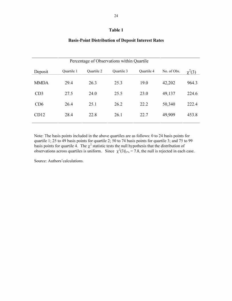
digits. In table 1, we give the proportion of observations falling within quarter-integer �buckets,�

where the first, second, third, and fourth quartiles represent deposit rates ending in 0 to 24, 25 to

49, 50 to 74, and 75 to 99 basis points, respectively. For all deposit types, the largest proportion

of rate observations is always within the first quartile of basis points and the smallest proportion

is always within the fourth quartile. As expected, these effects appear strongest for MMDAs.

The hypothesis that the quoted deposit rates are uniformly distributed across basis-point quartiles

is rejected at greater than the 1 percent level for every deposit type.

III.B Evidence of the Relative Stickiness of Whole-Digit Deposit Rates

As predicted by Theorem 2 and as illustrated in figure 2, a bank�s propensity to change

its deposit rate should be less sensitive to a given shock in its wholesale market funding rate when

the deposit rate is currently at an integer value. In this section, we investigate whether the data

support this notion of relative stickiness at whole-integer values. In testing this hypothesis, we

14

proxy the wholesale market rate by the LIBOR having the same maturity as the retail deposit.6 In

addition, we attempt to control for other sources of deposit rate stickiness that have been

identified in previous research. For a given change in market rates, Hannan and Berger (1991)

find evidence of greater MMDA rate stickiness for banks in more concentrated deposit markets.

Thus, in testing the propensity to change deposit rates, we include a measure of local deposit

market concentration -- the Herfindahl index of the local metropolitan statistical area.7 We also

control for the extent of disequilibrium between market and deposit rates by including a variable

that measures the spread between wholesale market and retail deposit rates.

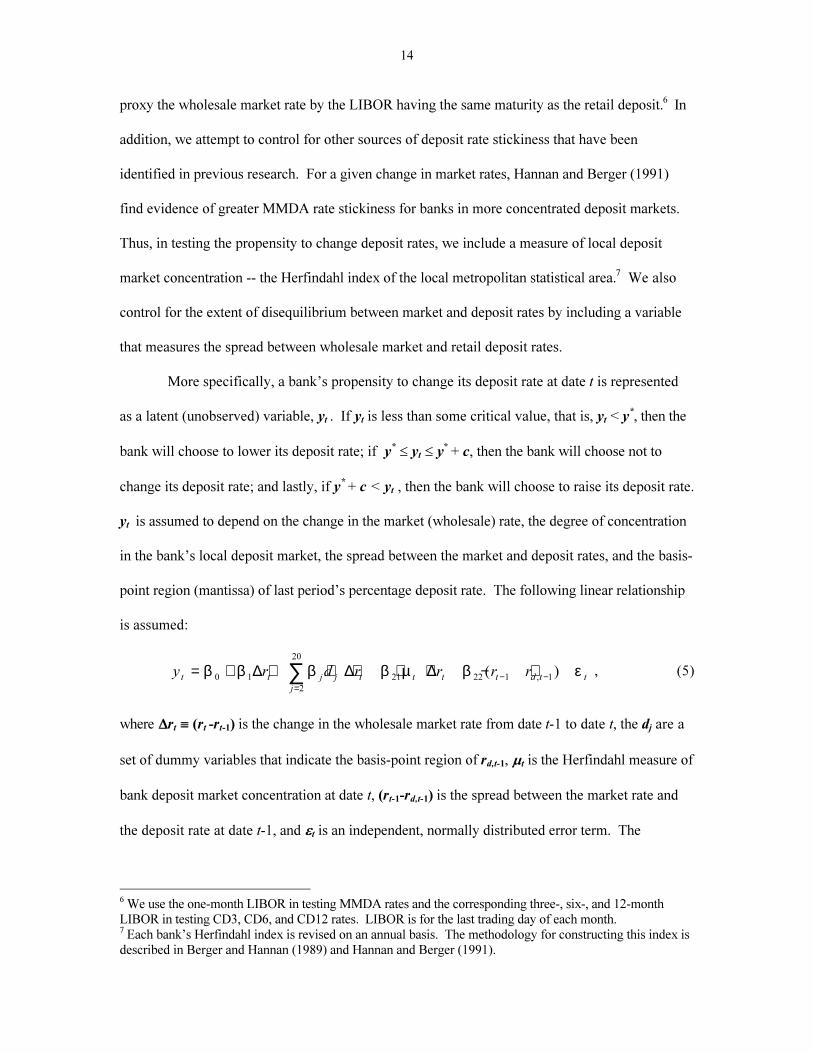
More specifically, a bank�s propensity to change its deposit rate at date t is represented

as a latent (unobserved) variable, yt . If yt is less than some critical value, that is, yt < y*, then the

bank will choose to lower its deposit rate; if y* £ yt £ y* + c, then the bank will choose not to

change its deposit rate; and lastly, if y* + c < yt , then the bank will choose to raise its deposit rate.

yt is assumed to depend on the change in the market (wholesale) rate, the degree of concentration

in the bank�s local deposit market, the spread between the market and deposit rates, and the basis-

point region (mantissa) of last period�s percentage deposit rate. The following linear relationship

is assumed:

y r d r r r rt t j j

j

t t t t d t t= + + ⋅ + ⋅ + − +=

− −∑β β β β µ β ε0 1

2

20

21 22 1 1∆ ∆ ∆ ( ), , (5)

where DDrt ºº (rt -rt-1) is the change in the wholesale market rate from date t-1 to date t, the dj are a

set of dummy variables that indicate the basis-point region of rd,t-1, mm t is the Herfindahl measure of

bank deposit market concentration at date t, (rt-1-rd,t-1) is the spread between the market rate and

the deposit rate at date t-1, and ee t is an independent, normally distributed error term. The

6 We use the one-month LIBOR in testing MMDA rates and the corresponding three-, six-, and 12-monthLIBOR in testing CD3, CD6, and CD12 rates. LIBOR is for the last trading day of each month.7 Each bank�s Herfindahl index is revised on an annual basis. The methodology for constructing this index isdescribed in Berger and Hannan (1989) and Hannan and Berger (1991).

15

inclusion of the set of dummy variables, dj, j = 2,...,20, will indicate whether rate stickiness

depends on the basis points of the previously quoted percentage deposit rate. Since the

histograms of MMDA and CD rates in figures 3 to 6 indicate spikes at every five basis points, the

basis-point region was divided into 20 subintervals, with the first being percentage rates having a

mantissa of 0 to 4 basis points, the second being 5 to 9 basis points, up to the twentieth region

being 95 to 99 basis points. The dummy variables dj , j = 2,...,20 take on the value of 1 if the

previous percentage deposit rate had a mantissa in the jth region, and 0 otherwise. Hence, for a

given change in the wholesale market rate, DDrt, the coefficient bbj measures the flexibility (lack of

stickiness) of rates having a mantissa in the jth region relative to rates having a mantissa in the

first region (0 to 4 basis points). Thus, a positive value for bbj , j = 2,...,20 indicates that the rates

in the first region (basically, the whole-integer level) are relatively stickier than rates in the jth

region.

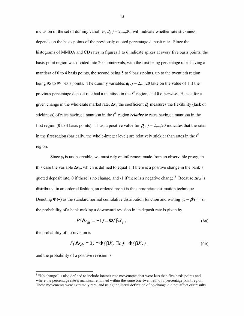
Since yt is unobservable, we must rely on inferences made from an observable proxy, in

this case the variable DDrdt, which is defined to equal 1 if there is a positive change in the bank�s

quoted deposit rate, 0 if there is no change, and -1 if there is a negative change.8 Because DDrdt is

distributed in an ordered fashion, an ordered probit is the appropriate estimation technique.

Denoting FF (··) as the standard normal cumulative distribution function and writing yt = bbXt + ee t,

the probability of a bank making a downward revision in its deposit rate is given by

P r Xdt t( ) ( )∆∆ ΦΦ= − =1 β , (6a)

the probability of no revision is

P r X c Xdt t t( ) ( ) ( )∆∆ ΦΦ ΦΦ= = + −0 β β , (6b)

and the probability of a positive revision is

8 �No change� is also defined to include interest rate movements that were less than five basis points andwhere the percentage rate�s mantissa remained within the same one-twentieth of a percentage point region.These movements were extremely rare, and using the literal definition of no change did not affect our results.

16

P r X cdt t( ) ( )∆∆ ΦΦ= = − +1 1 β . (6c)

Thus, the log-likelihood function is

ln ln[ ( )] ln[ ( ) ( )] ln[ ( )]L z X z c X X z c Xdt

N

t n t t u t= + + − + − +=∑

1

1ΦΦ ΦΦ ΦΦ ΦΦβ β β β , (7)

where zd, zn, and zu equal 1 if DDrdt equals -1, 0, and 1, respectively.

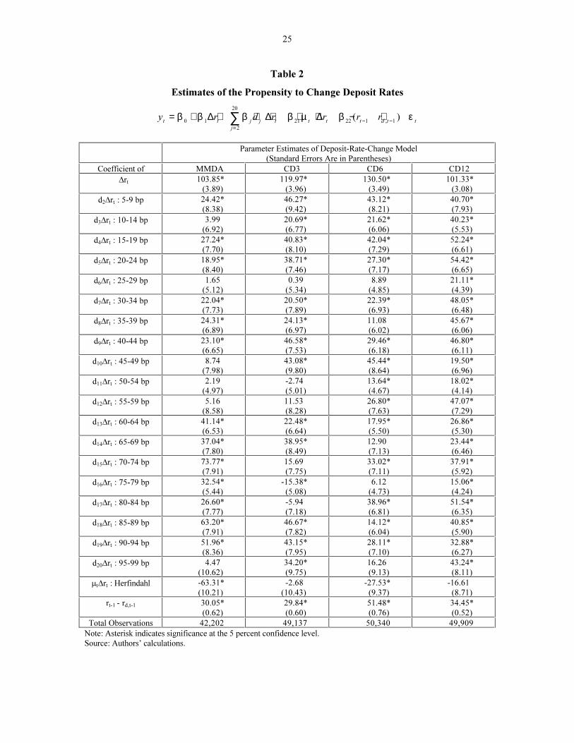
The estimation results are reported in table 2. For each deposit type, the parameter

estimates of the coefficients multiplying the market rate, DDrt, and the market/deposit-rate spread,

(rt-1-rd,t-1), have the expected positive signs and are highly significant. Consistent with Berger and

Hannan�s (1991) finding that deposits rates are stickier in more concentrated markets, the

coefficients of the Herfindahl index times the market rate change, mm t DDrt, are all negative, though

only statistically significant for MMDAs and CD6s. Of most interest to the hypothesis that rates

should be relatively stickier at whole digits are the coefficients of the basis-point dummy

variables times the market rate change, djDDrt , j = 2,...,20. With the sole exception of the CD3, the

point estimates of the coefficients of these variables are all positive, and most are statistically

significant (in fact, all are significant for the CD12). When lack of significance does occur, it is

often at the quarter, half, or three-quarter digit, i.e., the coefficients on variables d6DDrt, d11DDrt, and

d16DDrt. Taken together, these empirical results confirm the model�s prediction that deposit rates

are stickiest when set at whole-digit percentage rates, but that secondary stickiness also exists

when rates are set at quarter-digit levels.

III.C Evidence of a Propensity for Whole-Digit Deposit Rates at Higher Market Rates

Based on Theorem 2 and figure 2, a bank�s propensity to quote retail deposit rates at a

whole digit should increase as market rates rise. To test this hypothesis, we represent a bank�s

propensity to quote a whole-digit rate as another latent variable, wt. If wt is less than some critical

value, i.e., wt < w*, then the bank chooses not to quote a whole-digit percentage interest rate. If

17

instead wt ³ w*, then the bank chooses to quote a whole-digit rate. wt is assumed to take the

form

w rt t r t t t= + + + +β β β σ β µ ε0 1 2 3, , (8)

where rt is the market rate at date t, ssr,t is the standard deviation of the market rate, and mm t is a

measure of market concentration. Our theoretical model would predict a positive value for bb1, the

coefficient of the market rate, which we again proxy by LIBOR.9 Because the volatility of market

rates, ssr,t, tends to be positively correlated with the level of market rates, and greater volatility

could have an independent influence on the tendency to quote whole-digit rates, we also include a

proxy for interest rate volatility -- the annualized standard deviation of daily LIBOR during the

previous month.

In equation (8), a bank�s propensity to set rates at whole digits is also allowed to depend

on the level of deposit market concentration, mm t, which is proxied by the Herfindahl index of the

bank�s local deposit market. We include this variable for two reasons. First, to the extent that

market power affects the form of the deposit demand function faced by a bank, our model implies

that it may influence the bank�s profit-maximizing interest rate. In general, however, the effect of

market power on the propensity to set whole-digit rates is theoretically ambiguous, so that the

expected sign of bb3 is unclear. A second reason for the inclusion of mm t is to consider the

possibility that setting whole-digit interest rates could be a mechanism by which banks collude,

implicitly or explicitly, to maintain noncompetitive deposit rates. Such a collusive agreement

would be similar in spirit to the agreement by NASDAQ security dealers to trade at even eighths,

as alleged by Christie and Schultz (1994) and Christie, Harris, and Schultz (1994). Maintaining

whole-digit deposit rates might serve as a price-fixing mechanism that allows banks to exert

9 As before, we use LIBOR with a maturity equal to that of the corresponding retail deposit.

18

market power. Because the ability to maintain such an agreement would be more likely in a more

concentrated market, this hypothesis would imply a positive coefficient for bb3.

Since wt is unobserved, our tests rely on an observable proxy, namely, a variable that

equals 1 when the bank sets its deposit rate at a whole digit, and 0 otherwise. This implies a

probit model having the log-likelihood function

ln ( )ln[ ( )] ln[ ( )]L z X z Xw

t

N

t w t= − + −=∑ 1 1

1

Φ Φβ β , (9)

where zw equals 1 if the percentage deposit rate is at a whole integer level, and 0 otherwise.

The estimation results are given in table 3. With the possible exception of the CD3, there

is clear evidence that the propensity to set whole-digit rates increases with the level of market

rates. In addition, greater market rate volatility appears to increase the likelihood that CDs will

be set at whole rates. Finally, there is mixed evidence that whole-digit rates are more common in

more concentrated markets. In summary, these results support the theory�s prediction that whole-

digit rates are more likely as market rates rise.

19

III.D Evidence of a Propensity for Deposit-Rate Integer Changes at Higher Market Rates

Another implication of figure 2 is that when market rates are high, ceteris paribus, a

bank�s propensity to change its quoted interest rate should fall, since the optimal deposit rate is

likely to be only at whole-digit breakpoints, not points interior to whole-digit levels. However,

when market rates are high and a deposit rate change does occur, the deposit rate is likely to pass

from one integer level to another. More precisely, conditional on a rate change occurring, a

change where rates move from x.y percent to (x±1).z percent is more likely when market rates are

high. Conversely, a change where rates move from x.y percent to x.z percent is more likely when

market rates are low. We define the former movement as an integer change and the latter as a

non-integer change and consider a test of this implication of the model.

The proposition is tested in the following manner. Conditional on a deposit rate change

occurring, we examine whether an integer change is systematically related to the level of the

market rate rt, which we again proxy by the equivalent-maturity LIBOR. Because the volatility of

market rates, ssr,t, tends to rise at higher levels of rt, and because this would clearly tend to

increase the propensity for integer changes, we control for this effect by including the annualized

standard deviation of daily LIBOR for the previous month. Finally, for the same reasons given in

the previous section, the propensity for a bank to make integer changes is allowed to depend on its

Herfindahl index of market concentration, mm t. More specifically, we let vt be a latent variable such

that if vt < v*, any change that does occur will not be an integer change. However, if vt ³ v*, then

any change will be an integer change. vt is assumed to take the form

v rt t r t t t= + + + +β β β σ β µ ε0 1 2 3, . (10)

The estimation technique is again a probit model that uses only those observations on deposit

rates for which a change occurred.

20

The results are reported in table 4. Notice from the last row that integer changes

constitute approximately 24 to 29 percent of all deposit rate movements. Overall, the evidence in

the table provides strong support for the model�s prediction. Both higher market rates and greater

market rate volatility (the CD12 being an exception with regard to volatility) increase the

likelihood of an integer change. There is some indication that integer changes are less likely in

more concentrated markets, at least for CD6s and CD12s. This may be due to the greater deposit

rate stickiness found in those markets, a phenomenon that could reduce the likelihood of integer

movements.

IV. Conclusion

This paper examines banks� optimal deposit-rate-setting behavior when some customers

have limited recall. Taking seriously the experimental evidence that individuals recall odd-ending

numbers less accurately than even-ending numbers, and that expressing a number as odd-ending

increases the likelihood that it will be underestimated when recalled, we model deposit demand by

limited-recall customers as being a function of the floor of the percentage deposit interest rate.

Our analysis shows that it is optimal for banks to set their deposit rates either at a whole integer

or at an interior point that satisfies a specific first-order condition.

The model predicts that the likelihood of interest rates being set at a whole digit increases

with both the proportion of limited-recall consumers in the market and advances in the wholesale

market interest rate. Also, for a given market rate shock, the quoted deposit rate tends to be

stickier when it is currently at a whole digit than when it is not. Lastly, although deposit rates tend

to be stickier when market interest rates are high, if and when there is a change in the deposit rate,

the change tends to be larger, jumping from one whole digit to another. Our tests using monthly

21

MMDA and CD interest rates for over 500 individual banks during a 10-1/2-year period provide

strong corroborative evidence in support of the model�s implications.

Our finding that limited recall results in price stickiness has a potentially much broader

significance. Price stickiness is an important theme in macroeconomics. The literature on �menu

costs� posits that the presence of small direct costs of adjusting prices can result in price

stickiness that has a large real impact on the economy. However, evidence for the presence of

menu costs is derived mainly from evidence that prices remain unchanged. In contrast to the menu

cost literature, our theory assumes no cost of adjusting prices, per se, but nevertheless results in a

considerable degree of price stickiness. In addition, our theory implies that deposit rates (prices)

should be stickier when they start from (just below) a whole digit. This difference in stickiness,

which distinguishes our model from the menu cost approach, is in fact confirmed by our empirical

tests. A promising area for future research would be to examine the macroeconomic

consequences of price and interest rate stickiness generated by limited recall.

22

References

Ball, C., W. Torous, and A. Tschoegl (1985) �The Degree of Price Resolution: The Case of theGold Market,� Journal of Futures Markets 5, 29-43.

Berger, A. and T. Hannan (1989) �The Price-Concentration Relationship in Banking,� Review of

Economics and Statistics 71, 291-299.

Blinder, A. (1991) �Why Are Prices Sticky? Preliminary Results from an Interview Study,� American Economic Review: Papers and Proceedings 81, 89-96.

Brenner, G. and R. Brenner (1982) �Memory and Markets, or Why Are You Paying $2.99 for a Widget?� Journal of Business 55, 147-158.

Brown, S., P. Laux, and B. Schachter (1991) �On the Existence of an Optimal Tick Size,� Review

of Futures Markets 10, 50-72.

Christie, W. and P. Schultz (1994) �Why Do NASDAQ Market Makers Avoid Odd-Eighths Quotes?� Journal of Finance 49, 1813-1840.

Christie, W., J. Harris, and P. Schultz (1994) �Why Did NASDAQ Market Makers Stop Avoiding Odd-Eighths Quotes?� Journal of Finance 49, 1841-1860.

Colwell, P., P. Rushing, and K. Young (1994) �The Rounding of Appraisal Estimates,� Illinois

Real Estate Letter, Summer/Fall.

Davis, R., L. Korobow, and J. Wenninger (1987) �Bankers on Pricing Consumer Deposits,� Federal Reserve Bank of New York, Quarterly Review, Winter, 6-13.

Diebold, F. and S. Sharpe (1990) �Post-Deregulation Bank-Deposit-Rate Pricing: The Multivariate Dynamics,� Journal of Business and Economic Statistics 8, 281-291.

Friedman, L. (1967) �Psychological Pricing in the Food Industry,� in A. Phillips and O. Williamson, eds., Prices: Issues in Theory, Practice, and Public Policy, University of Pennsylvania Press, Philadelphia, 187-201.

Goodhart, C. and R. Curcio (1990) �Asset Price Discovery and Price Clustering in the Foreign Exchange Market,� London School of Economics, Working Paper.

Hannan, T. and A. Berger (1991) �The Rigidity of Prices: Evidence from the Banking Industry,� American Economic Review 81, 938-945.

Harris, L. (1991) �Stock Price Clustering and Discreteness,� Review of Financial Studies 4, 389-415.

23

Hutchison, D. and G. Pennacchi (1996) �Measuring Rents and Interest Rate Risk in Imperfect Financial Markets: The Case of Retail Bank Deposits,� Journal of Financial and

Quantitative Analysis (forthcoming).

Kashyap, A. (1995) �Sticky Prices: New Evidence from Retail Catalogs,� Quarterly Journal of

Economics 110, 245-274.

Neumark, D. and S. Sharpe (1992) �Market Structure and the Nature of Price Rigidity: Evidence from the Market for Consumer Deposits,� Quarterly Journal of Economics 107, 657-680.

Nierderhoffer, V. (1965) �Clustering of Stock Prices,� Operations Research 13, 258-265.

Osborne, M.F.M. (1962) �Periodic Structure in the Brownian Motion of Stock Prices,� Operations Research 10, 345-379.

Rosen, R. (1995) �What Goes Up Must Come Down? Asymmetries and Persistence in BankDeposit Rates,� Finance Department, Indiana University, mimeo.

Schindler, R. and A. Wiman (1989) �Effects of Odd Pricing on Price Recall,� Journal of

Business Research 19, 165-177.

Wisniewski, K. and R. Blattberg (1983) �Response Function Estimation Using UPC Scanner Data: An Analytical Approach to Demand Estimation under Dealing,� in F. Zufryden, ed., Advances and Practice of Marketing Science, Institute of Management Science, Providence, R.I., 300-311.

24

Table 1

Basis-Point Distribution of Deposit Interest Rates

Percentage of Observations within Quartile

Deposit Quartile 1 Quartile 2 Quartile 3 Quartile 4 No. of Obs. c2(3)

MMDA 29.4 26.3 25.3 19.0 42,202 964.3

CD3 27.5 24.0 25.5 23.0 49,137 224.6

CD6 26.4 25.1 26.2 22.2 50,340 222.4

CD12 28.4 22.8 26.1 22.7 49,909 453.8

Note: The basis points included in the above quartiles are as follows: 0 to 24 basis points forquartile 1; 25 to 49 basis points for quartile 2; 50 to 74 basis points for quartile 3; and 75 to 99

basis points for quartile 4. The c2 statistic tests the null hypothesis that the distribution of

observations across quartiles is uniform. Since c2(3)|1% = 7.8, the null is rejected in each case.

Source: Authors�calculations.

25

Table 2

Estimates of the Propensity to Change Deposit Rates

y r d r r r rt t j j

j

t t t t d t t= + + ⋅ + ⋅ + − +

=− −∑β β β β µ β ε

0 1

2

20

21 22 1 1∆ ∆ ∆ ( )

,

Parameter Estimates of Deposit-Rate-Change Model(Standard Errors Are in Parentheses)

Coefficient of MMDA CD3 CD6 CD12

Drt 103.85*(3.89)

119.97*(3.96)

130.50*(3.49)

101.33*(3.08)

d2Drt : 5-9 bp 24.42*(8.38)

46.27*(9.42)

43.12*(8.21)

40.70*(7.93)

d3Drt : 10-14 bp 3.99(6.92)

20.69*(6.77)

21.62*(6.06)

40.23*(5.53)

d4Drt : 15-19 bp 27.24*(7.70)

40.83*(8.10)

42.04*(7.29)

52.24*(6.61)

d5Drt : 20-24 bp 18.95*(8.40)

38.71*(7.46)

27.30*(7.17)

54.42*(6.65)

d6Drt : 25-29 bp 1.65(5.12)

0.39(5.34)

8.89(4.85)

21.11*(4.39)

d7Drt : 30-34 bp 22.04*(7.73)

20.50*(7.89)

22.39*(6.93)

48.05*(6.48)

d8Drt : 35-39 bp 24.31*(6.89)

24.13*(6.97)

11.08(6.02)

45.67*(6.06)

d9Drt : 40-44 bp 23.10*(6.65)

46.58*(7.53)

29.46*(6.18)

46.80*(6.11)

d10Drt : 45-49 bp 8.74(7.98)

43.08*(9.80)

45.44*(8.64)

19.50*(6.96)

d11Drt : 50-54 bp 2.19(4.97)

-2.74(5.01)

13.64*(4.67)

18.02*(4.14)

d12Drt : 55-59 bp 5.16(8.58)

11.53(8.28)

26.80*(7.63)

47.07*(7.29)

d13Drt : 60-64 bp 41.14*(6.53)

22.48*(6.64)

17.95*(5.50)

26.86*(5.30)

d14Drt : 65-69 bp 37.04*(7.80)

38.95*(8.49)

12.90(7.13)

23.44*(6.46)

d15Drt : 70-74 bp 73.77*(7.91)

15.69(7.75)

33.02*(7.11)

37.91*(5.92)

d16Drt : 75-79 bp 32.54*(5.44)

-15.38*(5.08)

6.12(4.73)

15.06*(4.24)

d17Drt : 80-84 bp 26.60*(7.77)

-5.94(7.18)

38.96*(6.81)

51.54*(6.35)

d18Drt : 85-89 bp 63.20*(7.91)

46.67*(7.82)

14.12*(6.04)

40.85*(5.90)

d19Drt : 90-94 bp 51.96*(8.36)

43.15*(7.95)

28.11*(7.10)

32.88*(6.27)

d20Drt : 95-99 bp 4.47(10.62)

34.20*(9.75)

16.26(9.13)

43.24*(8.11)

mtDrt : Herfindahl -63.31*(10.21)

-2.68(10.43)

-27.53*(9.37)

-16.61(8.71)

rt-1 - rd,t-1 30.05*(0.62)

29.84*(0.60)

51.48*(0.76)

34.45*(0.52)

Total Observations 42,202 49,137 50,340 49,909

Note: Asterisk indicates significance at the 5 percent confidence level.Source: Authors� calculations.

26

Table 3

Estimates of Propensity to Set Whole-Digit Deposit Rates

w rt t r t t t= + + + +β β β σ β µ ε0 1 2 3,

Parameter Estimates of Whole-Digit Deposit Rate Model(Standard Errors Are in Parentheses)

Coefficient of MMDA CD3 CD6 CD12

rt 0.0478*(0.0044)

0.0042(0.0038)

0.0113*(0.0038)

0.0368*(0.0034)

sr,t -0.1245(0.0652)

0.2362*(0.0790)

0.6003*(0.0796)

0.0388*(0.0144)

mt : Herfindahl 0.0704(0.0602)

0.1118(0.0585)

-0.0448(0.0614)

0.3646*(0.0552)

Total Observations 42,202 49,137 50,340 49,909

% Obs. at Whole Digit 15.84 13.44 11.60 14.16

Table 4

Estimates of Propensity for Integer Changes in Deposit Rates

v rt t r t t t= + + + +β β β σ β µ ε0 1 2 3,

Parameter Estimates of Model with Integer-Deposit-Rate Changes(Standard Errors Are in Parentheses)

Coefficient of MMDA CD3 CD6 CD12

rt 0.0465*(0.0056)

0.0509*(0.0044)

0.0276*(0.0040)

0.0824*(0.0041)

sr,t 1.2715*(0.0803)

1.5613*(0.0813)

1.7548*(0.0766)

-0.0553*(0.0182)

mt : Herfindahl -0.0308(0.0832)

-0.0372(0.0641)

-0.1519*(0.0610)

-0.5986*(0.0779)

Total Rate Changes 19,651 28,780 34,540 33,881

% Integer Changes 24.44 29.09 27.13 28.60

Note: Asterisk indicates significance at the 5 percent confidence level.Source: Authors� calculations.

Source: Authors’ calculations.

Source: Authors’ calculations.

Source: Authors’ calculations.