Baltic Tigers Facing the Middle-Income Trap? · Ernests Bordāns, Madis Teinemaa 1 Bachelor Thesis...
57
Ernests Bordāns, Madis Teinemaa 1 Bachelor Thesis Baltic Tigers Facing the Middle-Income Trap? Authors: Ernests Bordāns Madis Teinemaa Supervisor: Oļegs Krasnopjorovs May 2016 Riga
Transcript of Baltic Tigers Facing the Middle-Income Trap? · Ernests Bordāns, Madis Teinemaa 1 Bachelor Thesis...

Ernests Bordāns, Madis Teinemaa
1
Bachelor Thesis
Baltic Tigers Facing the Middle-Income Trap?
Authors:
Ernests Bordāns
Madis Teinemaa
Supervisor:
Oļegs Krasnopjorovs
May 2016
Riga

Ernests Bordāns, Madis Teinemaa
2
Table of Contents
Abstract ................................................................................................................................................... 4
1. Introduction .................................................................................................................................... 5
Research Questions ........................................................................................................................ 6
2. Literature Review ............................................................................................................................ 7
2.1. Theory of MIT ........................................................................................................................... 7
2.2. Middle income level definition in the literature ...................................................................... 8
2.3. Middle income trap definition in the literature ..................................................................... 10
2.4. Literature on MIT determinants ............................................................................................ 13
3. Methodology ................................................................................................................................. 14
3.1 Our MIT Definition ...................................................................................................................... 14
3.1.1. Setting the middle income level ......................................................................................... 15
3.1.2 Choosing the “trap” criteria ................................................................................................. 15
3.1.3 Other characteristics of our definition ................................................................................. 17
3.2 Estimating the MIT determinants and probability of MIT .......................................................... 18
3.2.1. Multivariate logistic panel data regressions ....................................................................... 18
3.2.2. Choosing the control variables ..................................................................................... 18
3.2.3. Fitting the model(s) ....................................................................................................... 19
3.2.4. Individual exogenous factors analysis ........................................................................... 21
3.3. Data description ......................................................................................................................... 21
4. Empirical results ................................................................................................................................ 23
4.1. Findings of the MIT .................................................................................................................... 23
4.2. Results of regression models with exogenous MIT probability determinants .......................... 28
4.2.1. Macroeconomic environment ............................................................................................ 28
4.2.2. Development ....................................................................................................................... 30
4.2.3. Governance ......................................................................................................................... 32
4.3. MIT predictions for Baltics ......................................................................................................... 35
5. Discussion of Results ......................................................................................................................... 38
5.1 Predicted probability for the Baltic States .................................................................................. 38
5.2. Performance of the Baltics in the context of previous literature MIT definitions ..................... 39
5.3. Discussion of key determinants of MIT: relevance for the Baltics ............................................. 41
5.3.1. Income level ........................................................................................................................ 41
5.3.2. Macro stability .................................................................................................................... 41
5.3.3. Competitiveness.................................................................................................................. 42
5.3.4. Economic structure ............................................................................................................. 43
5.3.5. Human capital ..................................................................................................................... 43

Ernests Bordāns, Madis Teinemaa
3
5.3.6. Income inequality ............................................................................................................... 44
5.3.7. Public sector performance .................................................................................................. 44
5.3.8. Corruption ........................................................................................................................... 45
6. Conclusions ....................................................................................................................................... 46
7. Reference list .................................................................................................................................... 48
8. Appendices ........................................................................................................................................ 52
Appendix A. All middle income level countries identified between 1960 and 2014. ........................ 52
Appendix B. All Middle Income Traps identified between 1960 and 2014. ...................................... 52
Appendix C. Prediction models ......................................................................................................... 53
Appendix D. Cross-correlation table of the main prediction model. ................................................. 54
Appendix E. Example of individual regressions. ................................................................................ 54
Appendix F. Estimated MIT probabilities using the main prediction model for all countries in
specific year. ..................................................................................................................................... 55
Appendix H. MIT predictions for Baltics with “HIC” and “MIC” scenario adjustments .................... 56
Appendix I. Predicted MIT probabilities for all countries in 2014. ................................................... 56
Appendix J. Data sources. ................................................................................................................. 57
Ernests Bordāns, Madis Teinemaa
4
Abstract
This paper studies the characteristics of middle income trap (MIT) and estimates the
probability of the Baltic Tigers facing it. We complement the existing literature in three ways.
First, we propose an original MIT definition considering major drawbacks of previous
researches and compiling unique country-specific benchmarks based on weighted average
income growth of trading partners. Second, we construct several multivariate panel data logit
models to study which economic, social and political factors could be associated with MIT.
Third, we are first to quantitatively assess the probability of the Baltic countries facing
MIT. Our results suggest the Baltic countries currently are not trapped since their GDP per
capita growth rate exceeds that of comparable middle-income countries, weighted average of
trading partners and the EU region; additionally, none of the existing literature’s MIT
definition suggests that any Baltic economy is trapped. Furthermore, the probability of them
facing a MIT is low (somewhat higher in Latvia and Lithuania than in Estonia), compared to
other European countries. However, MIT probability of the Baltic countries is likely to rise if
further income convergence with advanced countries will not be accompanied with structural
reforms. We find that quality of public institutions (especially government effectiveness and
control of corruption), business-friendly regulations, income equality, stable macroeconomic
environment, prudent fiscal policy as well as developments in higher education, innovation
and product sophistication are crucial to avoid MIT in the future.
Ernests Bordāns, Madis Teinemaa
5
1. Introduction
Even despite the deep economic recession in 2008-2009 the Baltic States have shown
impressive economic performance since the beginning of 21st century. Beating the odds of
many, Latvia, Estonia and Lithuania have managed to increase their GDP per capita levels (at
PPS) from 36%, 43% and 39% of the European Union average respectively in 2000, to 63%
in Latvia and 74% in Estonia and Lithuania respectively in 2014 (Eurostat, 2015). In truth,
this rapid catching up was experienced largely because the income gap between the Baltics
and the EU was so large (thus, the Baltics had relatively competitive labour market (lower
wages), higher marginal returns to capital, opportunity to import technologies etc.) and due
some short term economic growth boosts (e.g. credit boom). However, the post-crisis period
has experienced a considerable slowdown in the economic growth compared to pre-crisis
period, and many suggest that Baltic States might be facing the mysterious middle income
trap (MIT) (IMF, 2015; OECD, 2015).
Pundits suggest that we cannot expect Baltics to simply keep converging with the EU with
the same pace as before given a considerable change in their relative income and overall
macroeconomic environment, and remind that that the only European country that has
substantially changed its position in GDP per capita ranking in Europe is Ireland. Moreover,
there is no consensus about the existence of absolute convergence between countries globally
(Sala-i-Martin, 1996).
International Monetary Fund (IMF, 2015) and Bank of Latvia economists (Kasjanovs, 2015)
that have discussed the MIT as a threat to the Baltic economies, agree that the current
slowdown might not yet mean that we are trapped; however, it indicates a necessity for more
profound structural reforms. In a recent study, Staehr (2015) points specifically at the Baltic
States facing the risk of MIT; and Swedbank has identified necessity for more growth-
friendly government spending in Latvia to avoid the MIT (Strašuna, 2015).
Continued steady growth is a matter of policies and MIT literature suggests that countries at
similar development stage as the Baltic States need to revise their economic policy in order to
avoid economic slowdown (Ohno, 2009). We want to find out whether based on social and
economic indicators, that roughly represent the economic policies pursued, the Baltic States,
are ready to avoid the MIT and continue convergence with the European average income.

Ernests Bordāns, Madis Teinemaa
6
Even though pundits have conceptually agreed on what is and what might be causing the
middle income trap, there is no official definition for MIT. Apparently, it is something that
combines being at middle-income level and experiencing low economic growth. Different
researchers offer different numeric definitions for such situation; literature has agreed neither
on thresholds for middle income level, nor characteristics of trap. Thus, the first objective of
this paper is to review the literature on each of the component of MIT definition and propose
original definition that addresses the drawbacks in previous literature by offering country-
specific benchmarks. By applying our definition, we find which middle income countries
have historically been or currently are caught in MIT.
The second objective is to study the impact of different economic, social and political factors
on the probability of countries being caught in MIT. We construct several multivariate panel
data logit models to find factors that are consistently associated with MIT occurrence.
The third objective is to quantitatively assess the probability of each Baltic country facing the
MIT. This is achieved by fitting a highly significant multivariate panel data logit model that
takes into account all factors that are found to be the most significant during the research.
Research Questions
Hence, we aim at sequentially answering the following research questions:
1) Which countries have historically been or currently are caught in the
MIT?
2) What is the current probability of Baltic countries facing the MIT and
which Baltic country is most likely to get trapped?
3) Which factors are associated with MIT and what policies particularly
Baltic States should implement to avoid MIT?
To our best knowledge, no study taking into account so many explanatory factors and
quantitatively assessing the probability of countries facing the MIT has been carried out. By
answering our research questions we aim at being able to provide policy recommendations
for the Baltic States.
The remainder of the paper is structured as follows: section 2 offers a review of existing
literature by paying particular attention to the definition of MIT; section 3 describes the
methods used and process of quantitative data analysis; section 4 presents the findings of
Ernests Bordāns, Madis Teinemaa
7
MIT occurrence, results of estimated predicted probabilities for the Baltic States and impact
of exogenous factors; and section 5 offers discussion of results.
2. Literature Review
2.1. Theory of MIT
In their original paper Gill, Kharas and Bhattasali (2007) were the first to name and discuss
MIT as a potential threat to a continued East Asian countries’ growth to high income level.
They claimed that in order to continue to grow, the East Asian countries must develop
economies of scale by continuing to increase the share of high-technology products in their
immense international trade, improving the knowledge absorption capacities (via education,
property rights, competitiveness), building strong financial system, including peripheric
regions in trade networks and eliminating inequality. Since then, researchers have mostly
studied the MIT in the context of sustainability of East Asian “miracle”, and the slowdown of
Latin American and Middle East countries.
When defining the MIT, most papers refer to how Gill et.al. (2007) characterized it initially.
To their mind, country is caught in MIT at the point when it is not capable of outcompeting
lower-income countries with their factor prices and also not able to compete with the
technology and productivity of high-income countries. In other words, the strategy for
economic growth at low-income level is not so efficient at middle-income level anymore
(Kharas and Kohli, 2011).
The loss of competitiveness among middle-income countries can be explained by W. Arthur
Lewis (dual-sector) development model which states that low wages and imitated technology
may boost growth at the low-income economies by moving labor from labor-intensive
agricultural sector to more productive (and better paid) manufacturing; however, eventually,
with rising income, labor-intensive sectors become less competitive and marginal returns
from imitated technology decrease. Thus, further growth can only occur with technological
advancements based on innovation not imitation (Agenor, Canuto and Jelenic, 2012).
Similarly, Ohno (2009) proposes to view the economic development as a four-stage process
where slowdown can occur at any transition between the stages. In his view, the MIT occurs
when an economy is moving from light manufacturing, that is mostly established by FDI, to a
stage where local human capital is developed and share of high-quality production is
increasing.

Ernests Bordāns, Madis Teinemaa
8
It is important to note that because MIT has not been defined unambiguously and its
identification in most researches depends on the definition chosen by authors, we cannot be
fully sure that MIT is really a trap; i.e. Im and Rosenblatt (2013) conclude that even though it
can be observed that middle income countries rarely advance to high income levels and it is a
troubling issue, the growth and convergence patterns of middle income countries do not differ
that much from the usual path of convergence where human capital, infrastructure,
institutions, TFP and investments are crucial for absolute convergence. Similarly, skeptical
authors have shown middle income countries do not present signs of consistently lower
growth than low-income countries (Bulman, Eden and Nguyen, 2014).
Given that thus far no unified MIT definition exists, but acknowledging the determinative
impact that MIT definition has on any further research, in order to define the MIT we must
firstly, agree on “middle income level”, and secondly - on characteristics of trap. Further, we
review on what assumptions has previous literature been based; and what are the findings.
2.2. Middle income level definition in the literature
Generally, there are two ways how literature has approached definition of middle income
level – either with absolute
thresholds or relative thresholds that
allow absolute threshold to change
over time. Table 1 summarizes the
middle income level classifications
that previous MIT literature has
used1.
With regards to absolute income
level benchmarks, first thing to
notice is that these thresholds tend to
be very broad. E.g. according to
Felipe et.al. (2012) classification,
some upper-middle income countries
can be roughly six times richer than
the lower-middle income countries.
1 Felipe et.al. (2012) set benchmarks in 1990 prices; for convenience, we estimate these benchmarks in 2005 prices adjusting them by the historical inflation.
World Bank
$1'045 - $4'125 - $12'736 (2014$; GNI per capita)
Felipe, Abdon and Kumar (2012)
$2'988 - $10'833 - $17'557 (2005$; GDP per capita PPP)
Aiyar, Duval, Zhang, Puy, Wu (2013)
$2'000 - $15'000 (2005$; GDP per capita PPP)
Eichengreen (2012; 2014)
$10'000+ (2005$; GDP per capita PPP)
Woo (2012)
20%-55% of USA (GDP per capita PPP)
Robertson, Ye (2013)
8%-36% of USA (GDP per capita PPP)
Table 1 Middle income level classifications in literature
Created by the authors. Some sources distinguish higher
and lower middle income levels; in those the middle
number in the table is the threshold.
Ernests Bordāns, Madis Teinemaa
9
However, can we actually compare the situation in two so different countries, and can we
have the same policy recommendations for them? Moreover, the absolute thresholds hold
stable over time. Thus, theoretically we could e.g. identify that Honduras (GDP per capita in
1950s was above $2000) was in a MIT back in 1950s and 1960s. However, can we directly
compare the economic situation of Honduras during 1960s with that of Spain in 2010, which
is also believed to be trapped?
At the same time, this absolute threshold would mean that back in 1950s there were
practically no high-income economies. However, back in 1960s when the richest countries
were advancing to high-income levels (by absolute values) they lived in much poorer world
overall, with less developed trading partners, less foreign technologies to imitate and, thus,
determinants of their growth might have been different. So, can we apply their lessons to
nowadays world? Similarly, Rosenblatt et.al. (2013) points out that if we assume an absolute
threshold for middle income, then the majority of high income countries were trapped in MIT
in the 20th century because it took very long for them to advance to high-income. This raises
a question of whether a middle income trap is fully endogenous problem of countries and
being trapped or escaping is a question of their policies regardless of the time and income-
level of other countries, or is it dependent on how the country looks relatively to others?
Moreover, setting a precise absolute benchmark is even more ambiguous task.
MIT is assumed to be a point where a country is stuck because it has not transformed its
economy into a productivity-driven one and, thus, it can compete with neither low, nor high
income countries (Gill et.al., 2007). This definition inherently assumes that there are
wealthier and more productive countries in this world. Furthermore, wealth and
productiveness have grown substantially over the last 60 years e.g. one of the richest country
in the world, USA’s per-capita income grew more than three times between 1950 and 2010,
and consequently changed the assumption of what are “wealthier and more productive
countries” “with which the middle-income countries must compete”. In other words, the
income level that can be achieved by imitation of foreign technologies increases over time.
Following these logics, it seems obvious that for studying middle-income trap, we need a
definition of middle income that includes some dynamic, time-varying trend. However, using
a relative benchmark or a catch-up index as a threshold also raises serious ambiguity issues.
Firstly, relative benchmarks have been widely criticized because of their underlying
assumption of existence of absolute convergence, which does not have a robust empirical

Ernests Bordāns, Madis Teinemaa
10
proof (Sala-i-Martin 1996). World Bank (2012) and other researchers point out that – there
were 101 countries that had advanced to relative (to USA) middle income benchmark level
by 1960; however, only 13 of them had reached high income level by 2008; and five of those
are East Asian “miracles“ (Felipe et.al., 2012) (Rosenblatt et.al., 2013) (Woo, 2012). But can
we really say that all the rest are trapped, if they have experienced growth in absolute terms?
Woo (2012) acknowledges that as the income levels globally have been rising consistently
over the last centuries, some dynamic trend must be included in the definition of middle
income. He proposes a catch-up index benchmarked to the USA per capita GDP, defining
middle income countries as those with income level between 20 and 55% of USA’s. The
author analyzes data of 1960-2008 and finds that middle income countries tend to converge
among themselves (e.g. Latin America) but not catch up with the USA. This methodology
does not estimate a precise time period of trap and because of the wide range, we cannot
know whether the country was growing at the same pace throughout the whole time periods,
or maybe it did not grow during the first years and at one point - rocketed up. Moreover,
relative catch-up benchmarks imply that middle-income countries should grow faster than the
high-income countries. Some empirical findings support these claims; however, it is arguable
whether it is it right to assume that middle income country growing at the same pace as high
income is trapped forever.
2.3. Middle income trap definition in the literature
Once the benchmarks for middle income level are set (if at all), existing literature on MITs
offer us several ways how to identify traps. Generally, two approaches can be taken for
identifying traps – statistical methods or intuitive rules (of thumb).
With regards to intuitive methods, Felipe et.al. (2012) offer identifying countries in the MIT
as those that have spent more years as middle income countries than on average countries
historically have. They find that the median number of years it took on average for countries
to get through the middle income was 42 years. And thus, they estimate that 35 of 52 middle
income countries were trapped in 2010.
Advantages of this definition are that authors can estimate the average growth rate necessary
for countries to avoid MIT and also specific periods in history when different countries have
been trapped. However, this definition also has major flaws. Firstly, authors admit that the
number of years spent in middle income largely depend on the historical time period we look
at, i.e. the later country entered the lower-middle income level, the shorter time it spent there

Ernests Bordāns, Madis Teinemaa
11
on average, and nowadays countries tend to cross the absolute thresholds quicker. Secondly,
no consistent data is available for countries before 1950s, thus, we cannot know how long
before 1950 some countries had already been in the middle income level. Thirdly, authors’
methodology implies that there always must be countries in the MIT (those that are below
average growth) i.e. country can be considered to be trapped simply if it is growing slower
than others have been historically. And lastly, given that countries’ growth rates could
actually differ quite substantially over time such definition makes it almost impossible to
analyze the influence of specific exogenous factors on the probability of being trapped.
Eichengreen et.al. (2014) offer another intuitive method for identifying the MIT. They do not
define middle income, and simply look at all countries above 10000$ GDP per capita PPP
(2005-prices). By employing GDP per capita data starting from 1957 they look for points in
time (years) where a country after 7-year (t-7) average annual income growth of at least 3.5%
experiences a drop in the average growth for the next 7 years (t+7) by at least 2 percentage
points. The time “t” is identified as a slowdown. In case several years in a row are identified
as slowdowns, Chow test for these years is employed to find the most significant break point
in the growth rate. Eichengreen et.al. (2014) identify that most often slowdowns occur at 10
000 – 11 000$, 15 000 – 16 000$, and around 17 000$ GDP per capita PPP.
Advantage of this methodology is that it identifies years when the slowdown (trap) is the
most pronounced and, thus, should work well for studying which factors caused a slowdown.
However, the assumptions of this model raise many questions. Firstly, according to Penn
World Tables there were only 11 countries with income level above 10 000$ in 1956, thus,
this methodology rules out many possible subjects for study. Secondly, the benchmark of
3.5% for growth before the slowdown rules out all countries that have been in a trap for the
whole period and never achieved 3.5% growth (e.g. South Africa), and the value of this
benchmark seems arbitrary; third, the 2 percentage point growth slowdown is not well
justified. For instance, countries that have experienced GDP per capita growth of 10% and
now have slowed down to 8% would also be identified as being in a trap.
Using a statistical approach, Aiyar et.al. (2013) assumes middle income level to be 2000 –
15000$ GDP per capita PPP (2005-prices). He gathers consistent data for 138 countries
between 1955 and 2009. First, expected GDP per capita growth is predicted for each year by
regressing GDP per capita growth on physical capital stock, human capital index and lagged
per capita income. Then they identify MIT by looking at the distribution of differences

Ernests Bordāns, Madis Teinemaa
12
between the expected growth of economy and the actual; country is identified to be in a trap
if the residuals for certain years are in the 20th percentile of all residuals calculated (i.e. the
expected growth was substantially larger than the actual). Authors divided the sample into
eleven 5-year periods and looked for those 5-year periods that met their definition; 11% of
them were found to be in a MIT. They also found that middle income countries experience
the slowdowns more frequently than other countries.
The obvious flaw of this methodology is that its accuracy depends on the assumptions of their
theoretical growth model (that GDP growth can be predicted by those three factors). Thus, we
face the joint-hypothesis problem (when we cannot tell whether their theoretical growth
model is wrong or whether MIT do not exist). Moreover, this model would not identify a
MIT in countries where MIT is caused or is reflected in low investment in physical and
human capital. Hence, it is more of a simple test for the model.
Robertson and Ye (2013) offers another statistical model for defining the MIT by looking
particularly at the long-run growth of economies. They assume middle income level to be
between 8 – 36% of USA’s (assuming it to be the world’s technology frontier), and for a
country to “qualify” as MIT country, its long-run per capita income forecast should lie in the
middle income range and the distribution of the differences between the country’s log income
level and USA’s log income level should be stationary (i.e. countries’ income levels are not
converging). They find that out of 46 middle income countries, 19 are trapped. To our mind,
the main flaw of this definition of MIT is that it does not allow any convergence; thus, it
might not identify countries that are growing very slowly but have some convergence; or
countries that are diverging from the USA.
Furthermore, apart from defining the MIT, there is fair amount of literature focusing on
simply determining economic slowdowns. One of the most straightforward ways to try to
estimate slowdowns is by using econometric tests that look for structural breaks in series e.g.
the Chow test or Quandt-Andrews test; however, these tests generally tell us less about the
direction of the break and they identify individual years, rather than a time period that could
be assumed MIT. Berg, Ostry and Zettelmeyer (2012) offer a relatively more sophisticated
method for identifying breaks in the growth. They define a period that starts with a statistical
upbreak in growth (2-3% growth) and ends with a downbreak in growth (or the end of
sample) as a “growth spell”. The breaks are identified by minimizing the sum of squared
residuals between average growth rates before and after the break using the Monte Carlo
Ernests Bordāns, Madis Teinemaa
13
simulation. Depending on the minimum years set between the breaks (5 or 8), authors
identify 174 to 280 breaks (including both upbreaks and downbreaks) starting from 1950s.
2.4. Literature on MIT determinants
In a qualitative paper, Kharas et.al. (2011) suggest that in order to avoid MIT, apart from the
prerequisites of manufacturing industry becoming more capital and skill intensive and
services as share of GDP increasing, the key strategy should be development of the domestic
demand that is necessary as a platform for domestic companies with global ambitions.
Relatedly, income inequality might be a reason for country to be stuck in a MIT, as unequal
income distribution can lead to domestic demand growing slower than the GDP, and at some
point country can face a slowdown because of underinvestment in human capital. Kharas
et.al. (2011) recommends three key policy changes – specialization, structural reforms for
improving TFP, and decentralization and privatization.
Researchers have employed different intuitive arithmetic and statistical estimation methods
like probit, logit and proportional hazard models for studying the determinants of MIT. Aiyar
et.al. (2013) employ probit regressions (with binary variable whether a country in a specific
year is in MIT or not) and Bayesian averaging as robustness tests, and estimate the impact of
42 different explanatory variables (including lagged and differenced values). They find that
better rule of law, less government involvement, lower regulations, lower dependency ratio,
higher trade openness, higher investments, services and agriculture as share of GDP, lower
capital inflows, larger public debt, smaller distance to trade, higher regional integration and
higher export diversification are associated with lower probability of MIT. By employing
similar econometric methodology, Eichengreen et.al. (2014; 2011) complements the literature
by finding that lower MIT probability is also associated with higher consumption, lower
fertility rates, lower employment share in manufacturing, higher share of population with
secondary and tertiary education and more high-technology exports.
Furthermore, Berg et.al. (2012) employ proportional hazard model to estimate the expected
length of (previously described) “growth spells” (including lagged and differenced factor
values). They find that growth is likely to persist if there is current account surplus, more
sophisticated exports, openness to FDI, income equality, democratic institutions and
macroeconomic stability. Agenor et.al. (2015) employ an overlapping generations simulation
model, and find that MIT occurs because of misallocation of talent, low productivity growth,
Ernests Bordāns, Madis Teinemaa
14
inefficient labor market, lack of property rights and weak (especially – advanced (e.g. IT))
infrastructure.
All policy recommendations in the literature require structural reforms. Felipe et.al. (2012)
emphasize the potential of a country for further structural changes. They estimate revealed
comparative advantage (RCA) and apply Hausmann and Klinger (2006) methodology to
export data. They find that number of products with RCA, share of core products in exports,
product sophistication and uniqueness of country’s exports are associated with lower risk of
MIT.
Notably, we identify considerable gaps and drawbacks in the previous literature on MIT
determinants. Firstly, all previous papers that have used logit or probit estimations have had
possible econometric estimations biases, i.e. Aiyar et.al.(2013) and Eichengreen et.al. (2014)
do not attempt fitting multivariate regression models that would include more control
variables that previous economic growth literature has identified to be relevant; their
regression specifications may feature large multicollinearity; and regression specifications
include just few significant variables (the insignificant ones are not excluded). Secondly, vast
majority of the previous literature has focused simply on identifying the significant factors;
however, none has attempted to quantify the actual probability of certain countries facing the
MIT or assessed the magnitude of the effect of certain factors on a particular country.
3. Methodology
3.1 Our MIT Definition
Credibility of any findings of this paper are dependent on a successful and appropriate
definition of the MIT in context of the Baltic States. As can be seen, the definition of middle
income trap is ambiguous and we identify all methodologies to have major flaws. The key
characteristics that the definition should inhabit in order to be used for our quantitative
analysis are (1) ability to capture a precise time period when the slowdown occurs, (2) trap
should differ from a short term economic slowdown, (3) countries identified as middle
income level must be comparable (at a similar development stage), (4) the definition must
take into account global, as well as regional macroeconomic environment (other country
income levels and growth) and (5) most importantly, the definition of middle income trap
must correspond as much as possible to how the researchers have agreed to characterize it –
country stuck between competitive low-wage and high-productivity status. Our key premise
is that country can be considered trapped if it is growing slower than it should be.
Ernests Bordāns, Madis Teinemaa
15
We offer an intuitive middle income trap definition that we believe solves most of the
problems identified previously, and that is specifically adjusted for the purpose of our
research – to study the Baltic States.
3.1.1. Setting the middle income level
Firstly, we must be sure that we have a comparable set of countries in our study sample and
that we can compare these countries over time. As showed by Felipe et.al. (2012) countries at
the same absolute income levels have performed substantially different over time, growing
much slower historically than countries at the same income level are growing nowadays.
Keeping that in mind, we choose to use relative benchmarks for determining middle income
countries, and these benchmarks are set accordingly, so that Baltic countries qualify as
middle income countries. We define relative income ranges as percentages of the USA’s
income level (assuming USA to be the World economic leader for the whole time period
observed (Robertson et.al., 2013)).
As discussed previously, researchers have chosen to use very different relative middle
income level benchmarks. In the context of MIT, Woo (2012) explains that income level of
15-60% of the USA features almost exactly the same set of countries throughout time since
1960s. Considering this and the fact that income level benchmark at 15% of the USA ensures
that all Baltic countries are identified to be middle income level for the whole period since
their data is observed (since 1990s) we set the bottom benchmark for middle income level at
15% of the USA (that is approximately 2270$ at PPP 2005 $ in 1960 and 6402$ in 2014).
Next, we choose 70% of the USA GDP per capita as the upper benchmark for middle income
level because that represents approximately the average income level of the European Union
over the time, and we assume that being above the average income level of the one of the
richest regions in the world (EU) would imply that country is above the middle income.
Baltic States started off in 1990s with the income level at PPP of around 20% of USA and
now are approximately halfway through our middle income definition. Setting the respective
middle income level benchmarks ensures us that almost half of the countries are European
and most African countries are excluded (list of all countries identified as middle income at
some point can be found in Appendix A).
3.1.2 Choosing the “trap” criteria
According to our proposed MIT definition, a country is trapped in a certain year if it fulfils
three country-specific criteria related to its GDP per capita growth rate.
Firstly, we wish to compare each country’s growth rate with other countries at similar

Ernests Bordāns, Madis Teinemaa
16
economic development stage, to see if the specific country is performing as well as other
countries that are also in the transition between labour and technology-intensive industries.
However, even within our defined middle income level range, countries at the poles of the
defined range have fairly different growth trends over time. Thus, in order to be sure that we
compare growth rates of countries across comparable sets, we divide middle-income
countries into four groups according to their income level – (1) countries at income level of
15%-20% of the USA, (2) at 20%-30%, (3) at 30%-50% and (4) at 50%-70% of the USA (list
of countries in each range may change every year). These income level intervals were chosen
(a) to ensure enough observations in each group every year; (b) to make sure that each
interval is not too wide and we can expect each set of countries to be similar; and (c) because
in recent years all Baltic countries belong to the same (30%-50% of USA) income level
interval.
Secondly, keeping in mind that growth rates differ across regions, we compare each
country’s growth rate with its respective region’s average growth rate. According to World
Bank classification we divide countries into the following regions – East Asia and Pacific,
Europe and Central Asia, European Union (partly overlaps with Europe and Central Asia),
Middle East & North Africa & South Asia, Sub-Saharan Africa, Latin America. Most middle
income trap definitions offered by previous researchers do not take into account how the
external macroeconomic environment impacts country’s performance; however, we believe
that it is important to control for external factors when studying which internal factors are
associated with MIT. And we believe that regional growth is a better proxy for external
macroeconomic environment than the World growth rate. Moreover, comparing middle
income countries growth rates with region’s average growth rate (despite the fact that the
regions also include countries at much different income levels) is justifiable because
according to the underlying MIT theory, countries that are in MIT should be growing slower
than both low and high income countries (as they can compete neither with low-wage
countries, nor more productive high-income countries).
Thirdly, we compare each country’s growth rate with the weighted average growth rate of its
trading partners’ in the specific year (weighted by the share of total exports). We believe that
having a country-specific benchmark is particularly important, because firstly, the trading
partners’ growth accounts for external shocks even better than regional growth rate (countries
located in periphery areas of their regions might not be affected from regional developments
as significantly as from its trading partners); secondly, trading partners’ growth rate is an
Ernests Bordāns, Madis Teinemaa
17
approximate benchmark of external demand and if country is not able to keep up with the
growth in trading partners, it might indicate that there is an issue with country’s
competitiveness.
To our best knowledge we are the first to create unique country-specific benchmarks for
researching middle income traps.
To summarize, our proposed MIT definition is as follows: we consider a country be trapped
in middle income during a specific year if its GDP per capita lies in the range of 15-70% of
the USA’s income level, and its GDP per capita growth rate is lower than a) the average
growth rate of other countries globally in its respective income level range (15-20%, 20-30%,
30-50% and 50-70% of the USA), 2) its respective region’s average growth, and 3) weighted
average growth of each country’s trading partners.
3.1.3 Other characteristics of our definition
The key advantage of using all three growth benchmarks lies in the fact that we use all of
them together and, thus, account for many limitations that each of the three benchmarks
would have if they were used individually and exclusively. If a country is growing slower
than each of the benchmark, we can be more certain that the growth of this country is lower
than it should be.
Similarly, we need several growth benchmarks to avoid a situation when half of the countries
would be trapped “by definition”. By comparing countries growth rates not only to other
middle income countries, we avoid situations when fast-growing middle income countries
would be considered trapped just because other middle income countries are growing even
faster (a flaw of Felipe et.al., (2012) methodology). Moreover, our definition does not assume
that there must definitely be an absolute convergence with the USA.
By using Hodrick-Prescott filter for GDP per capita values (described further in
methodology), we remove impact from economic cycles and record slowdown as a middle
income trap only when it is related to a long term growth trend. Moreover, we can identify a
country to be in MIT even if we do not have long historical GDP per capita data (as is the
case for the Baltics).
Nevertheless, we acknowledge that using the USA as a benchmark may be challenged, as this
approach assumes that countries at e.g. 50% of the USA’s income level in 1960s had the
same priorities as countries at 50% income level nowadays; however, it can be the case that
countries at the same relative income level in 1960s were still less developed and required

Ernests Bordāns, Madis Teinemaa
18
different strategy.
Moreover, we identify few cases when a country was caught in MIT for just one year. Such
finding may seem unintuitive as MIT is usually associated with more persistent long term
economic trends; however, we still include such observations because given that our GDP per
capita data is smoothed, it is unlikely that a country was identified to be in MIT due to one-
off event; it rather indicates that this country was on the edge of MIT.
3.2 Estimating the MIT determinants and probability of MIT
In order to estimate the probability of the Baltics facing the MIT and quantitatively assess the
impact of different explanatory factors on the probability of MIT we (1) choose control
variables for initial assessment of significance of different factors, (2) construct several
multivariate panel data logit models, (3) predict the probability of MIT using these models,
and (4) study the impact of individual factors by estimating their significance and consistency
of the impact across different model specifications.
3.2.1. Multivariate logistic panel data regressions
We employ multivariate panel data logit regressions in order to quantitatively assess the
impact of different factors on the probability of MIT and also predict the probability given
values of factors for each country. A binary variable indicating whether country in the
specific year was trapped or not is always used as the dependent variable.
We choose to perform random effect regressions. Firstly, Hausman specification test implies
that performing random effect estimations is appropriate for our data (Hausman and
McFadden, 1984); and secondly, fixed effect estimations automatically omit many countries
with zero variance in the dependent variable (e.g. countries that have never been trapped).
Furthermore, because all of our factors are continuous (not categorical) variables, estimated
marginal effects of our logit regressions can be misleading and not precise (Williams, 2015).
Hence, instead of estimating the marginal effects we manually adjust the factors of interest
and look at what is the change of predicted probability given different values for explanatory
variables. Further in our paper we test our prediction models in the described manner, by
altering some of the explanatory factors for the Baltic States.
3.2.2. Choosing the control variables
We cannot fully rely on previous literature when proposing our control variables because,
firstly, middle income trap literature is currently still very limited and inconclusive with

Ernests Bordāns, Madis Teinemaa
19
regards to its findings; secondly, even economic growth literature is largely indecisive about
which factors have consistently significant influence on economic growth (Levine and
Renelt, 1992) and, thirdly, our middle income trap definition is original and it is worth testing
as many variables as possible.
Findings of cross-country economic growth research are extremely sensitive to the
specification of regression model; thus, researchers often find contradicting coefficient signs
for the same factors and no clear consensus on the right model specification exists (Durlauf
and Quah, 1999) (Levine, 1992).
Nevertheless, most economists agree that univariate regressions can be misleading and
individual factors should always be studied by using a set of relevant control variables,
moreover, there should be some robustness checks (Hosmer, Lemeshow and Sturdivant,
2000) (Sala-i-Matin, 1997). After surveying the literature we find that the most often used
control variables in economic growth research are level of GDP per capita, investment share
in GDP, population growth, some human capital measure, proxy for trade openness, fertility,
world growth, government size and dummies for time periods (but rarely all of them are used
together) (Levine and Renelt, 1991).
We choose our control variables based on the following criteria: 1) they must have been used
as control variables in previous literature and found to be consistently significant, 2) all
chosen control variables must be significant when regressed together and they must maintain
their significance in majority of regressions with other factors added to the model, 3) they
must have low cross-correlation, 4) they must have sufficient amount of observations in our
dataset (starting from 1960s), and 5) their influence on MIT risk must have a clear causality.
After testing different factors, we find that GDP per capita, investment level, tertiary
education enrolment rate, trade openness and government spending as a share of GDP meets
all of our five criteria. Population growth, fertility and dummies for time periods often were
not significant when regressed together with other control variables. We do not consider
world growth rate as a control variable because it is indirectly included in our MIT definition.
3.2.3. Fitting the model(s)
Firstly, we want to restrict the number of factors for further consideration for inclusion in the
prediction models. After choosing five control variables we perform a preliminary assessment
of all the rest factors in our dataset. We perform logistic regressions using the five control
variables and adding all other variables one by one as the sixth explanatory variable to the
Ernests Bordāns, Madis Teinemaa
20
model (we do not perform univariate regressions at all). We consider a variable for further
inclusion in the main regression model if its p-value in the regression with control variables is
below 0.25 (similar approach for choosing candidates for group regressions is proposed by
Bursac, Gauss, Williams and Hosmer (2008).
Secondly, we fit the regression model using a stepwise selection procedure (adding variables
to the control variables in the model one by one and eliminating any variable that was added
previously if it turns insignificant (there are too many variables for using a backwards
selection in our case)). However, when using stepwise selection, the model that we end up
with is very dependent on what are the first variables that we add to the model and on which
we build it2. Hence, we repeat the stepwise selection procedure numerous times, each time
starting by different variables as the first ones to be considered in the model. Following the
recommendations in literature (Peng, Lee and Ingersoll, 2002) (Hoetker, 2007) we base
selection of the best model on the following criteria: 1) all variables included in the model
must be significant at p=0.053, 2) we consider the Wald Chi-Square goodness of fit test when
comparing similar models, 3) we validate how precise are the predicted probabilities of the
models for those observations that are actually trapped or not trapped, 4) we consider cross-
correlation between the variables in order to avoid multicollinearity (Appendix D), 5) we
include those variables that have sufficient amount of historic observations, and 6) we want
to have variables representing different categories (e.g. institutions, economic structure,
human capital etc.) in order to be sure that the model does not miss any crucial factors.
For robustness check we fit eight additional multivariate prediction models by largely
following the same described conditions of a good model; however, we compromise for one of
the conditions – for instance, including variables with less observations. The alternative
models’ predicted probabilities are less precise than for the main prediction model, they have
fewer explanatory variables and different number of observations; however, all variables are
still significant. Variables that are included in the all prediction models can be seen in Appendix
C, with our main prediction model marked as Model 1.
2 This appears because, firstly, there is still some cross-correlation between the variables, thus, the coefficients
interact between themselves and, secondly, because we are analysing such a long time period, different variables
observations might not overlap and once we add a variable to the model which has less observations than other
variables in the model it influences the sample. 3 Our main prediction model includes two variables significant at 90% level, to compromise for other good
characteristics of the model.
Ernests Bordāns, Madis Teinemaa
21
3.2.4. Individual exogenous factors analysis
The fitted models allow us to make some conclusions about those variables that are included
in the model; however, we would still like to analyse also variables that did not fit in the
models (they may still be relevant factors and may not be included in the models e.g. because
of too low number of observations). Thus, we follow Sala-i-Martin (1997) and Levine (1992)
and employ each variable in many different model specifications by using different sets of
control variables. The robustness of the impact can be assessed by judging in how many of
the regression specifications each variable was found significant.
Each variable in our dataset is regressed in 15 different regression specifications. In our
results, we present in how many of the 15 regressions (as percentage) each variable was
significant and with what sign.
For choosing the 15 regression specifications we follow Levine (1991) approach (who is
analysing robustness of FDI impact on economic growth). This implies having a set of fixed
control variables and adding additional relevant variables one by one (and thus having
additional regression model when each variable is added). The variables that are added
additionally to the five control variables are those variables that are included in the main
prediction model. Additionally, we regress each variable of interest by adding it to our main
model and four of the alternative models. Appendix E presents an example of our approach to
analysing each variable of interest (in this case - population growth)4.
3.3. Data description
Our data covers 152 countries for the period of 1960-2014. However, among these only 68
countries have been at middle income level at some point during our study time period, see
Appendix A for countries and periods under investigation. We follow Aiyar et.al.(2013) and
Eichengreen et.al.(2014) and exclude resource-exporter countries whose resource extraction
between 1960 and 2013 exceeds 20% of GNI on average5 based on data of Natural resources
depletion (as % of GNI) (WDI, 2015). Similarly as Felipe et.al. (2012), we also exclude
microstates (that we define as those with average population of less than 250 000 between
4 Detailed results (similar to Appendix E) on all other individual regressions are available upon request. We do
not attach all regression outputs here because of the large number of such estimation tables. 5 Countries that we exclude due to their resource richness are Angola, Azerbaijan, Bahrain, Brunei, Darussalam,
Bhutan, Congo, Rep., Gabon, Iraq, Kazakhstan, Kuwait, Libya, Nigeria, Oman, Qatar, Saudi Arabia,
Turkmenistan, Trinidad and Tobago, Uzbekistan
Ernests Bordāns, Madis Teinemaa
22
1960 and 2014) from further analysis6. We base all calculations of GDP per capita and
growth rates on data from a single database (Penn World Tables 7.1)7. The data sample that is
finally used for our analysis includes 2154 annual observations.
Following Eichengreen et.al.(2014) we intended to use seven-year average growth rates (t+/-
3 years) for cross-country growth rate comparisons, assuming that 7 years is period of
economic cycle, so that the smoothed growth would represent income growth based in
fundamentals. However, as in that case we would lose the growth rates of last three years, we
smooth our GDP per capita data using Hodrick-Prescott (HP) filter8. Moreover, we calculate
regional growth rates by weighing them by total GDP of countries in each region.
We create a dataset with annual data on the relative wealth and growth of each country’s
export partners (weighted by the amount of trade), in order to create country specific
benchmarks for our MIT definition and use trading partners’ relative wealth as one of our
factor in quantitative analysis, (IMF Direction of Trade Statistics database, 2016). To our
knowledge we are the first to study middle income traps using such specific dataset. The
weighted average trading partners’ data is compiled by assembling the annual export values
between all countries in our dataset from 1960 till 2014, computing weights for each country/
counterparty/year treble (e.g. Estonia’s proportional weight as Latvia’s export partner in
2014), and calculating the weighted average GDP per capita of trading partners and weighted
average trading partners’ growth in each year between 1960-2014.
Additionally to absolute values of our factors, we estimate the average value of each factor
based on all middle income countries in specific year, and then – estimate what is the value of
each country’s factor relatively to all middle income country average in that year (e.g. how
large was Latvia’s tertiary education enrolment rates in 1997 compared to average enrolment
6 Countries that we exclude are Aruba, Andorra, American Samoa, Antigua and Barbuda, Belize, Bermuda,
Brunei Darussalam, Curacao, Cayman Islands, Dominica, Faeroe Islands, Micronesia, Fed. Sts., Grenada,
Greenland, Guam, Isle of Man, Kiribati, St. Kitts and Nevis, St. Lucia, Liechtenstein, St. Martin (French part),
Monaco, Maldives, Marshall Islands, New Caledonia, Palau, French Polynesia, San Marino, Sao Tome and
Principe, Sint Maarten (Dutch part), Seychelles, Tonga, Tuvalu, St. Vincent and the Grenadines, Virgin Islands
(U.S.), Vanuatu Samoa
7 This database (PWT 7.1) features GDP per capita in constant 2005 prices for time period 1950-2010 and is
used by most middle income trap researchers (Eichengreen et.al., 2014) (Aiyar et.al., 2013). In order to be able
to also study the years of 2010 – 2014 (which are not covered) for the missing years we apply the growth rates
of GDP per capita PPP at constant prices data from the World Bank WDI database, and thus, get uninterrupted
GDP per capita data until 2014 8 We set the smoothing parameter 𝜆 at 21, in order to maximize the correlation between the estimated 7-year
average growth rate and HP-filtered GDP per capita growth rate.
Ernests Bordāns, Madis Teinemaa
23
rates among all middle income countries in 1997). Given that our study covers such a long
time period, considerable political, social and economic developments that have taken place
globally over time can have an influence on the findings of important factors (Levine and
Zervos, 1993). A bias in results can be caused e.g. by the fact that countries that had
relatively high human capital back in 1960s (and arguably – back then it caused a positive
effect on economic growth) at the same time had relatively low level of human capital if
compared to nowadays standards (as education enrolment rates have increased globally);
hence, some factors are less comparable over time. The estimated relative factor values do
not completely substitute the absolute values of each factor in our quantitative estimations;
they are used as robustness checks and we report results from all regressions - with relative
and absolute values of each factor.
Some factors (e.g. GINI index, Economic Freedom Index before 2000, BTI index and other)
are not observed in every year; hence, in order not to lose observations, we estimate the
missing observations by taking the average value of the closest existing observations.
Additionally, for the purpose of consistency, when studying exogenous factors impact, we
use a dataset where the values of all independent factors are included as averages of the
actual values of current and previous three years. Similar approach by lagging explanatory
variables is used by Aiyar et.al. (2013). We believe that such approach is more appropriate in
our research because, firstly, we are using smoothed GDP per capita data, and, secondly, we
are interested in finding the impact of sustained, structural problems in some of the factors
(not short term fluctuations) and these problems should be pronounced enough to also be
observed when averaged over several years.
The list of explanatory factors whose impact on the MIT we test can be found in Appendix J.
4. Empirical results
4.1. Findings of the MIT
Out of 2154 total middle income level countries observations for time period of 1960 – 2014,
689 (32%) are trapped. Our observed frequency is lower than e.g. for Felipe et.al. (2012) who
assumed that country is trapped if it grows through middle income level in more years than
other countries on average (which should yield approximately 50% frequency); however, our
frequency is substantially higher than was found by Aiyar et.al. (2013) who estimated it to be
around 11%. Note, however, that MIT probability cannot be compared directly to other
papers as the MIT definitions are different.

Ernests Bordāns, Madis Teinemaa
24
We find that the Baltic countries currently are not caught in the MIT; and among European
countries, Spain, Croatia, Cyprus, Portugal, Greece, Italy and Slovenia are currently trapped
(Italy slipped back into middle income level from high income level in 2010, see Appendix
A). Figures 2 below shows that the Baltic States have been avoiding the MIT since 1994 with
a great confidence beating all three middle income trap growth thresholds (regional, trading
partners and other middle income countries growth rates). Nevertheless, the economic
recession has had a significant influence on all three Baltic States growth rates, and Latvia’s
growth rate during 2009-2012 dropped somewhat below that of trading partners.
Frequency of middle income trap is different among regions; during the years of 1960-2014
Latin American countries were caught in trap in around 45% of all observations. Moreover,
most Latin American countries were trapped during the years of 1960-1988 (see Figure 3).
Such finding is consistent with previous literature. Without naming it “middle income trap”
Cimoli and Correa (2002) describe Latin America being caught in a “low growth trap” due to
their transition period. East Asia and Pacific region (middle income) countries have been
performing exceptionally well throughout our study period (MIT frequency has been just
11%), and apart from featuring some of the largest success stories of middle income countries
historically (e.g. South Korea and Singapore), also other countries have avoided prolonged
economic slowdowns, except for New Zealand in 1980s – 1990s. The average frequency of
MITs observed in the EU between 1960 and 2014 is 25%.
Our identified middle income traps usually occur for several consecutive years, and that is
consistent with the theoretical assumption that middle income trap is more than a short term
economic slowdown, and country can be caught in a bad equilibrium for a prolonged time
period. Hence, having identified long term periods of unreasonably low growth, we should be
able find the right causes of MIT.
MIT frequency has not been constant over time (see Figure 1a). Particularly, during the years
of mid-1960s to 1980 the frequency of slowdowns dropped on average well below 30%.
However, between 1980 and 2000 middle income traps occurred relatively more often (one of
the reason can be the collapse of USSR and “new” trapped middle income countries entered
the dataset); and then, together with the global economic boom the MIT frequency dropped
again in early 2000s.

Ernests Bordāns, Madis Teinemaa
25
Notably, countries at income level of 32.5-40% of the USA has had a considerably higher
frequency of MITs than at other income levels (see Figure 1b) This is a relevant finding given
that Latvia and Lithuania are currently at around 33% and 37% of USA income level
respectively.
Countries at income level of around 65-85% relatively to their trading partners on average
have experienced traps less often than countries at lower or higher income levels relatively to
their trading partners; that suggests that decreased wealth gap between home country and
trading partners might not be causing MIT per se. Estonia’s and Lithuania’s wealth relatively
to their trading partners is almost 70%; whereas, for Latvia - around 62%.
Figure 1 Frequency of MIT by years, absolute and relative income levels.
Created by the authors.

Ernests Bordāns, Madis Teinemaa
26
Figure 2 Baltic countries GDP PPP per capita growth rates compared to MIT definition
thresholds (income growth of trading partners, region and average of middle income countries
in specific income range where the country belongs to).
Created by the authors.

Ernests Bordāns, Madis Teinemaa
27
Country/Year
19
60
19
61
19
62
19
63
19
64
19
65
19
66
19
67
19
68
19
69
19
70
19
71
19
72
19
73
19
74
19
75
19
76
19
77
19
78
19
79
19
80
19
81
19
82
19
83
19
84
19
85
19
86
19
87
19
88
19
89
19
90
19
91
19
92
19
93
19
94
19
95
19
96
19
97
19
98
19
99
20
00
20
01
20
02
20
03
20
04
20
05
20
06
20
07
20
08
20
09
20
10
20
11
20
12
20
13
20
14
GreeceCyprusPortugalSpainTurkeyPolandRomaniaHungaryMacedoniaBulgariaCroatiaRussiaIrelandUKItalySlovakIAEstoniaSloveniaCzech Rep.SerbiaUkraineAlbaniaAustriaBelarusFinlandFranceLatviaLithuaniaMontenegroJamaicaVenezuelaArgentinaEl SalvadorUruguayPeruChileEcuadorGuatemalaMexicoBrazilCosta RicaSurinameColombiaNicaraguaBarbadosBoliviaPanamaDominican R.New ZealandSingaporeThailandMacaoChinaHong Kong JapanKorea, Rep.MalaysiaAlgeriaIranLebanonJordanIsraelDjiboutiMaltaTunisiaSouth AfricaEq. GuineaMauritius
ME
, N
A,
S.
Asia
Ea
st A
sia
an
d P
acif
icL
atin
Am
eric
aE
uro
pe
an
d C
en
tra
l A
sia
Afr
ica
Figure 3 Middle Income Traps from 1960 – 2014.
Created by the authors. Grey colour represents either missing GDP per capita data or the country being outside the middle
income level. Green colour represents a middle income country that is not trapped, red colour – a trapped middle income
country.
Ernests Bordāns, Madis Teinemaa
28
4.2. Results of regression models with exogenous MIT probability determinants
Appendix C presents the significance and signs of factors that are included in our prediction
models; in addition, Tables 2, 3, 4 present the findings on factors that were excluded from the
prediction models but which we analysed individually by employing in different regression
specifications (we also analyse individually all variables that were included in the prediction
models and report these results in Tables 2, 3, 4). In the Tables we indicate in how many of
the 15 regression specifications (as percentage) each variable of interest was significant; if
significant, what was the estimated impact on probability of MIT; and whether the variable
was significant when included in the main regression model. Moreover, we also show
whether the performance of the Baltic States (in 2014) in each factor differs significantly (at
5% significance) from the average values of other countries in the middle and high income
level in 2014 and show the results in the same tables9.
4.2.1. Macroeconomic environment
Income level
We witness that countries with lower GDP per capita levels are less likely to fall into trap
even when controlling for other factors. Impact is significant in almost all of our group
regressions including our main MIT prediction model. These findings for GDP per capita
impact on MIT likelihood are in line with vast evidence that has been found for conditional β-
convergence throughout different research approaches (Islam, 2003) (Quah, 1995) (Sala-i-
Martin, 1996).
Moreover, we find that higher income level relative to country’s trading partners has a
positive and significant impact on the probability of MIT when it is included in main
regression specification. Similar conclusion was reached by Arora and Vamvakidis (2005).
Hence, even though literature on convergence indicates that globally there could be absolute
divergence (Sala-i-Martin, 1996), trading intensively with wealthy economies can help
economy to avoid the MIT.
Macroeconomic stability
We find that favourable macroeconomic environment characterized by low inflation, low
standard deviation of inflation (our proxy for standard deviation of inflation is an Economic
Freedom index which is high if the standard deviation of inflation is low), higher budget
9 For some factors our dataset does not cover year of 2014; in that cases the latest available data is taken.
Ernests Bordāns, Madis Teinemaa
29
balance, monetary stability and lower price of capital has a significant and robust impact on
decreasing the probability of being caught in MIT (Table 2). This finding is consistent with
literature (Barro, 1996).
Economic structure
Higher investment rate has is significantly associated with lower probability of MIT and this
factor is significant in 93% of our regression specifications (including the main regression
model). We also find that higher government expenditure (% of GDP) increases the
probability of getting trapped in all 100% regression specifications. These findings are
consistent with that of Aiyar et.al. (2013). Regarding GDP structure on production side, we
find that only share of agriculture has a significant and negative impact on the probability of
MIT in most regression specifications. We find that industry as share of GDP is not
significantly related to middle income trap probability in most of the regression
specifications; however, the average share of industry as % of GDP in high and middle
income countries is also not statistically significantly different (see Table 2).
Competitiveness
We find that higher compensation as a share of total costs and pay-and-productivity relation
has a robust and significant impact on lowering the probability of MIT. Moreover, higher real
effective exchange rate proves to have a significant impact on increasing the probability of
MIT in about half of the regression specifications.
International trade and investments
Higher trade openness, lower trade barriers and tariffs have a robust and significant impact on
decreasing the probability of MIT. Moreover, we find that large current account deficits are
associated with higher MIT probability. Although, higher foreign direct investments have a
significant effect on decreasing the probability of MIT in 87% of regression specifications
(including the main model) (when used as an absolute value), when FDI is included in the
main regression model as a relative value it proves to be significant with increasing the
probability of MIT. Notably, many trade openness proxies (freedom to trade internationally
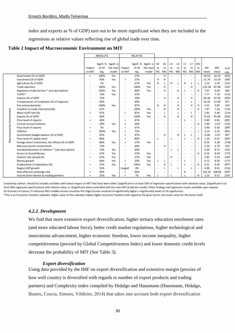
Ernests Bordāns, Madis Teinemaa
30
index and exports as % of GDP) turn out to be more significant when they are included in the
regressions as relative values reflecting rise of global trade over time.
4.2.2. Development
We find that more extensive export diversification, higher tertiary education enrolment rates
(and more educated labour force), better credit market regulations, higher technological and
innovations advancement, higher economic freedom, lower income inequality, higher
competitiveness (proxied by Global Competitiveness Index) and lower domestic credit levels
decrease the probability of MIT (See Table 3).
Export diversification
Using data provided by the IMF on export diversification and extensive margin (proxies of
how well country is diversified with regards to number of export products and trading
partners) and Complexity index compiled by Hidalgo and Hausmann (Hausmann, Hidalgo,
Bustos, Coscia, Simoes, Yildirim, 2014) that takes into account both export diversification
Table 2 Impact of Macroeconomic Environment on MIT
Government (% of GDP) + 100% Yes - 27% - H - - - - - 18.53 16.43 2031
Investment (% of GDP) - 93% Yes + 27% H H - - - - - 21.74 23.19 1987
Agriculture (% of GDP) - 7% - 67% Yes H L H L H L L 1.53 5.93 1537
Trade openness - 100% Yes - 100% Yes - H - - - H - 125.39 87.08 2147
Regulatory trade barriers * (see description) - 100% Yes - 80% Yes - H - H L - H 7.67 6.69 830
Tariffs* - 73% Yes - 67% - - - - - - - 7.77 7.70 1712
Imports (% of GDP) - 73% - 33% - H - H - H - 64.46 47.49 2033
Compensation of employees (% of expense) - 93% - 40% - - - L - L - 16.45 22.60 871
Pay and productivity - 100% Yes - 87% H H - H - H H 4.31 3.87 419
Freedom to trade internationally - 67% - 100% Yes - H - H - - H 7.87 7.26 1714
Mean tariff rate (%) + 67% + 87% Yes - L - L - L - 2.81 5.46 1116
Exports (% of GDP) - 60% - 100% Yes - H - H - H - 72.62 45.89 2033
Price level of imports + 40% + 87% - - - - L - - 0.89 0.85 2097
Current account balance - 29% Yes + 40% - - - - - - H 2.90 -2.67 1531
Price level of exports + 7% + 67% - - - - - - - 0.90 0.93 2097
Inflation + 100% Yes + 73% - - - - - - L 2.14 5.32 1851
Government budget balance (% of GDP) - 87% + 47% - H - H L L - -0.44 -3.07 857
Price level of capital stock + 86% + 80% L - L - L - H 1.24 0.91 2097
Foreign direct investment, net inflows (% of GDP) - 86% Yes + 27% Yes - - - - - - - 8.55 4.28 1738
Macroeconomic environment - 73% - 60% - H - - - - - 5.24 4.79 419
Standard deviation of inflation * (see description) - 73% Yes - 40% - - L L - - - 9.20 8.71 1761
Access to Sound Money - 67% Yes - 47% Yes - - - - - - H 9.25 8.59 1772
Interest rate spread (%) + 67% Yes - 27% Yes - - H - - - - 2.85 5.43 1367
Money growth - 60% Yes + 20% Yes L L - - L - - 9.12 8.92 1717
Employment of population (%) + 47% Yes + 100% Yes - H L - L - H 0.51 0.42 2077
Region GDP growth - 53% Insignif. 0% - L - L - L - 0.00 0.01 2154
Real effective exchange rate + 40% + 60% - - - - H - - 101.42 108.00 2097Income level relative to trading partners + 21% Yes + 7% Yes L - L - L - H 1.53 0.57 2147
EE=Estonia LV=Latvia LT=Lithuania MIC=middle income countries HIC=high income countries H=significantly higher L=significantly lower at 5% significance.
*This is an Economic Freedom subindex. Higher value of this subindex implies higher economic freedom with regard to the given factor, but lower value for the factor itself.
Created by authors. Result list includes variables with robust impact on MIT that have been either 1)significant in at least 50% of regression specifications with absolute value; 2)significant in at
least 50% regression specifications with relative value; or 3)significant when controlled with the main MIT prediction model. Other findings and regression results available upon request.
HIC
vs
MIC
HIC
mean
MIC
mean# of
obs.
Mac
roec
ono
mic
Env
iro
nmen
t
EE
vs
HIC
EE
vs
MIC
LV
vs
HIC
LV
vs
MIC
LT
vs
HIC
LT
vs
MIC
ABSOLUTE RELATIVE
Impact
on MIT
Signif. %
of all
reg.
Signif. in
the main
model
Impact
on MIT
Signif. %
of all
reg.
Signif. in
the main
model
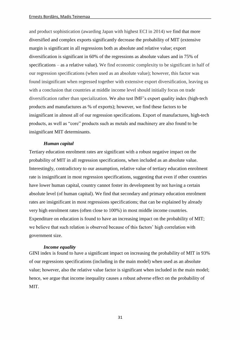
Ernests Bordāns, Madis Teinemaa
31
and product sophistication (awarding Japan with highest ECI in 2014) we find that more
diversified and complex exports significantly decrease the probability of MIT (extensive
margin is significant in all regressions both as absolute and relative value; export
diversification is significant in 60% of the regressions as absolute values and in 75% of
specifications – as a relative value). We find economic complexity to be significant in half of
our regression specifications (when used as an absolute value); however, this factor was
found insignificant when regressed together with extensive export diversification, leaving us
with a conclusion that countries at middle income level should initially focus on trade
diversification rather than specialization. We also test IMF’s export quality index (high-tech
products and manufactures as % of exports); however, we find these factors to be
insignificant in almost all of our regression specifications. Export of manufactures, high-tech
products, as well as “core” products such as metals and machinery are also found to be
insignificant MIT determinants.
Human capital
Tertiary education enrolment rates are significant with a robust negative impact on the
probability of MIT in all regression specifications, when included as an absolute value.
Interestingly, contradictory to our assumption, relative value of tertiary education enrolment
rate is insignificant in most regression specifications, suggesting that even if other countries
have lower human capital, country cannot foster its development by not having a certain
absolute level (of human capital). We find that secondary and primary education enrolment
rates are insignificant in most regressions specifications; that can be explained by already
very high enrolment rates (often close to 100%) in most middle income countries.
Expenditure on education is found to have an increasing impact on the probability of MIT;
we believe that such relation is observed because of this factors’ high correlation with
government size.
Income equality
GINI index is found to have a significant impact on increasing the probability of MIT in 93%
of our regressions specifications (including in the main model) when used as an absolute
value; however, also the relative value factor is significant when included in the main model;
hence, we argue that income inequality causes a robust adverse effect on the probability of
MIT.
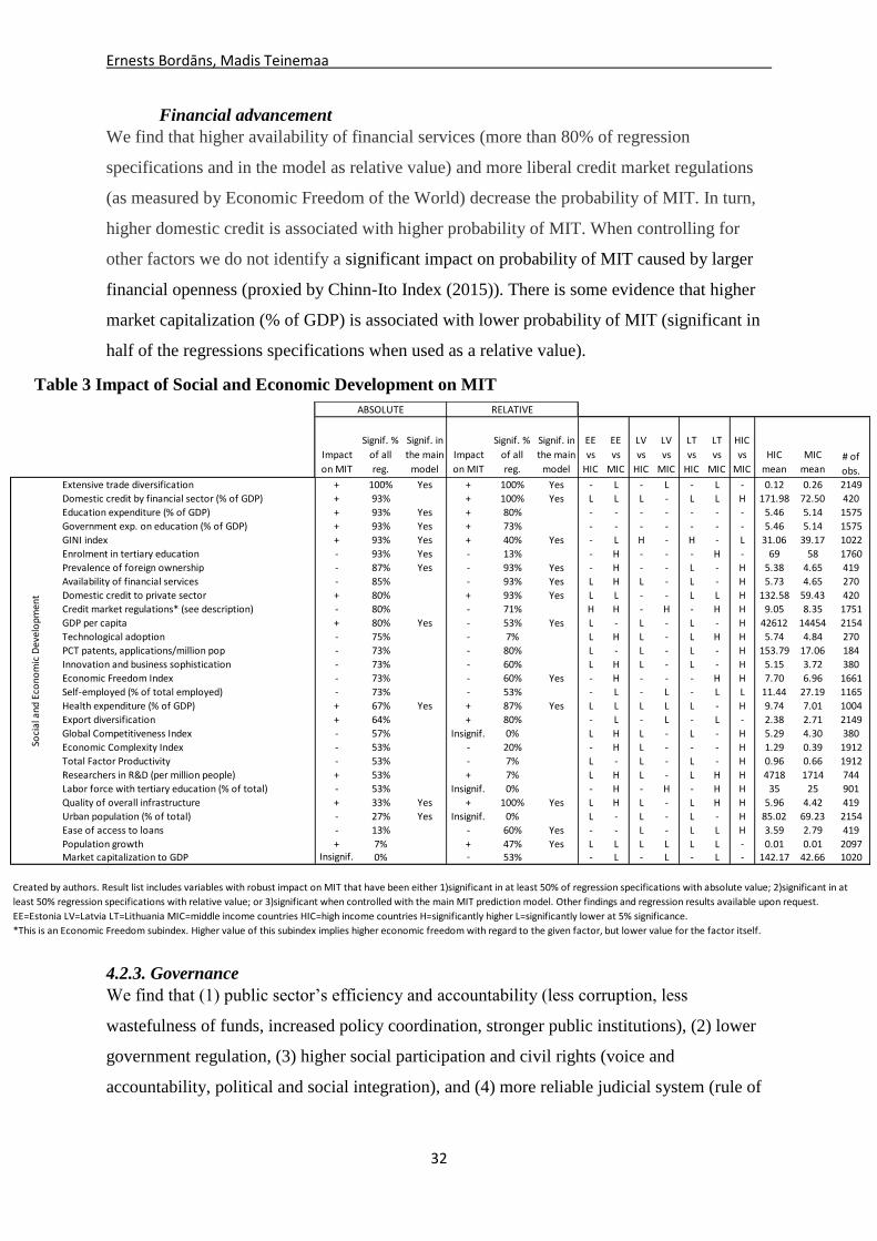
Ernests Bordāns, Madis Teinemaa
32
Financial advancement
We find that higher availability of financial services (more than 80% of regression
specifications and in the model as relative value) and more liberal credit market regulations
(as measured by Economic Freedom of the World) decrease the probability of MIT. In turn,
higher domestic credit is associated with higher probability of MIT. When controlling for
other factors we do not identify a significant impact on probability of MIT caused by larger
financial openness (proxied by Chinn-Ito Index (2015)). There is some evidence that higher
market capitalization (% of GDP) is associated with lower probability of MIT (significant in
half of the regressions specifications when used as a relative value).
4.2.3. Governance
We find that (1) public sector’s efficiency and accountability (less corruption, less
wastefulness of funds, increased policy coordination, stronger public institutions), (2) lower
government regulation, (3) higher social participation and civil rights (voice and
accountability, political and social integration), and (4) more reliable judicial system (rule of
Table 3 Impact of Social and Economic Development on MIT
Extensive trade diversification + 100% Yes + 100% Yes - L - L - L - 0.12 0.26 2149
Domestic credit by financial sector (% of GDP) + 93% + 100% Yes L L L - L L H 171.98 72.50 420
Education expenditure (% of GDP) + 93% Yes + 80% - - - - - - - 5.46 5.14 1575
Government exp. on education (% of GDP) + 93% Yes + 73% - - - - - - - 5.46 5.14 1575
GINI index + 93% Yes + 40% Yes - L H - H - L 31.06 39.17 1022
Enrolment in tertiary education - 93% Yes - 13% - H - - - H - 69 58 1760
Prevalence of foreign ownership - 87% Yes - 93% Yes - H - - L - H 5.38 4.65 419
Availability of financial services - 85% - 93% Yes L H L - L - H 5.73 4.65 270
Domestic credit to private sector + 80% + 93% Yes L L - - L L H 132.58 59.43 420
Credit market regulations* (see description) - 80% - 71% H H - H - H H 9.05 8.35 1751
GDP per capita + 80% Yes - 53% Yes L - L - L - H 42612 14454 2154
Technological adoption - 75% - 7% L H L - L H H 5.74 4.84 270
PCT patents, applications/million pop - 73% - 80% L - L - L - H 153.79 17.06 184
Innovation and business sophistication - 73% - 60% L H L - L - H 5.15 3.72 380
Economic Freedom Index - 73% - 60% Yes - H - - - H H 7.70 6.96 1661
Self-employed (% of total employed) - 73% - 53% - L - L - L L 11.44 27.19 1165
Health expenditure (% of GDP) + 67% Yes + 87% Yes L L L L L - H 9.74 7.01 1004
Export diversification + 64% + 80% - L - L - L - 2.38 2.71 2149
Global Competitiveness Index - 57% Insignif. 0% L H L - L - H 5.29 4.30 380
Economic Complexity Index - 53% - 20% - H L - - - H 1.29 0.39 1912
Total Factor Productivity - 53% - 7% L - L - L - H 0.96 0.66 1912
Researchers in R&D (per million people) + 53% + 7% L H L - L H H 4718 1714 744
Labor force with tertiary education (% of total) - 53% Insignif. 0% - H - H - H H 35 25 901
Quality of overall infrastructure + 33% Yes + 100% Yes L H L - L H H 5.96 4.42 419
Urban population (% of total) - 27% Yes Insignif. 0% L - L - L - H 85.02 69.23 2154
Ease of access to loans - 13% - 60% Yes - - L - L L H 3.59 2.79 419
Population growth + 7% + 47% Yes L L L L L L - 0.01 0.01 2097Market capitalization to GDP Insignif. 0% - 53% - L - L - L - 142.17 42.66 1020
EE=Estonia LV=Latvia LT=Lithuania MIC=middle income countries HIC=high income countries H=significantly higher L=significantly lower at 5% significance.
Created by authors. Result list includes variables with robust impact on MIT that have been either 1)significant in at least 50% of regression specifications with absolute value; 2)significant in at
least 50% regression specifications with relative value; or 3)significant when controlled with the main MIT prediction model. Other findings and regression results available upon request.
*This is an Economic Freedom subindex. Higher value of this subindex implies higher economic freedom with regard to the given factor, but lower value for the factor itself.
ABSOLUTE RELATIVE
Impact
on MIT
Signif. %
of all
reg.
Signif. in
the main
model
Impact
on MIT
Signif. %
of all
reg.
Signif. in
the main
model
HIC
vs
MIC
HIC
mean
MIC
mean# of
obs.
Soci
al a
nd E
cono
mic
Dev
elo
pmen
t
EE
vs
HIC
EE
vs
MIC
LV
vs
HIC
LV
vs
MIC
LT
vs
HIC
LT
vs
MIC
Ernests Bordāns, Madis Teinemaa
33
law, stronger property rights, efficiency of settling disputes) have robust and significant
impact on decreasing the probability of MIT (see Table 4).
Quality of public institutions, government efficiency, resource efficiency and wastefulness of
government spending have all been found to have a significant impact on the probability of
MIT in most regression specifications including the main model (either as absolute or relative
value).
We find higher control of corruption and improved anti-corruption policy to have a robust
and significant impact in decreasing the probability of MIT, as these factors are significant
also when included in the main regressions model.
We find that in order to avoid MIT, country should achieve higher economic freedom
(measured by Economic Freedom Index), have less (but more efficient) regulations and less
obstacles for starting business. Luckily, Baltics are performing significantly better than other
middle income countries on average in terms of business regulations, ease of doing business
and especially - wage flexibility.
Our findings suggest that tax policy can have a significant impact on the probability of MIT.
Direct taxation (specifically top marginal tax and tax on income, profits and capital gains)
increase MIT probability, while higher taxation of goods and services decrease it.

Ernests Bordāns, Madis Teinemaa
34
Table 4 Impact of Governance on MIT
Cooperation in labor-employer relations - 100% Yes - 100% Yes - H L H L - H 5.24 4.20 419
Diversion of public funds - 100% Yes - 100% Yes L H L - L - H 5.59 3.35 419
Wastefulness of government spending - 100% Yes - 100% Yes - H L - L - H 4.17 3.01 419
Burden of government regulation - 100% Yes - 100% Yes - H - - L - H 3.74 3.11 419
Voice and accountability - 100% Yes - 100% Yes - H - H - H H 1.15 0.25 973
Government efficiency - 100% Yes - 93% Yes - H L - L - H 4.58 3.43 419
Control of corruption - 100% Yes - 67% L H L - L - H 1.76 0.06 973
Legal system & property rights - 93% Yes - 100% Yes L H L H L H H 7.88 5.60 1627
Government effectiveness - 93% - 93% L H L H L H H 1.64 0.30 973
Resource efficiency - 93% - 87% Yes - H - - - H - 8.31 5.99 389
Protection of property rights - 93% Yes - 60% L H L - L - H 8.03 5.30 826
Market Economy Status Index - 100% Yes - 47% - H - H - H H 8.45 7.04 389
Ethical behavior of firms - 93% - 100% Yes L H L - L - H 5.88 4.02 419
Corporate ethics - 93% - 100% Yes L H L - L - H 5.88 4.02 419
Institutions - 93% - 100% Yes L H L - L - H 5.40 3.92 419
Ethics and corruption - 93% Yes - 20% L H L - L - H 5.38 3.40 419
Efficiency of legal framework in settling disputes - 92% Yes - 86% Yes L H L L L - H 5.16 3.52 308
Effect of taxation on incentives to invest - 91% - 67% Yes - H - - L - H 4.23 3.54 142
Anti-corruption policy - 87% - 87% Yes - H - - - H - 7.81 5.54 389
Rule of law (WGI) - 93% - 87% L H L H L H H 1.60 0.13 973
Efficienct use of talent - 93% - 80% Yes - H L H L H H 5.06 3.98 419
Judicial independence (WEF) - 80% - 100% Yes - H L - L - H 5.88 3.80 419
Black market exchange rates* (see description below) - 87% - 93% Yes - - - - - - H 132.58 59.43 1776
Policy coordination - 80% Yes - 40% - H L - - H H 9.44 6.50 389
Political and social integration - 86% - 73% - H - - - H - 4.35 6.48 389
Sustainability - 86% - 13% - H - H - H - 7.88 6.32 389
Welfare regime - 85% - 60% H H - H - H H 7.91 6.71 389
Civil rights - 80% - 87% Yes H H H H H H - 5.38 6.98 389
Accountability - 73% Yes - 80% Yes L H L - L - H 5.21 4.46 419
No. of days to start a business - 80% - 20% - - - - H - - 10.84 29.95 401
Organization of the market and competition - 79% - 73% - H - H - H - 8.63 7.55 389
Public institutions - 67% Yes - 80% Yes L H L - L - H 5.36 3.81 419
Flexibility of wage determination - 73% - 73% Yes H H H H H H - 4.50 4.80 419
BTI Status Index (democracy and market liberalism) - 73% - 47% H H - H H H - 6.58 7.12 389
Rule of law (BTI) - 67% - 60% H H - H H H - 5.05 6.59 389
Social capital - 67% - 27% H H - - H H - 5.44 6.30 389
Regulation* (see description) - 67% - 47% Yes - H - H - H H 7.80 6.91 1614
Country capacity to retain talent - 64% - 20% L - L - L L H 4.83 3.27 142
Irregular payments and bribes - 54% - 13% L H L - L - H 6.03 4.18 270
Taxes on goods and services (% of revenue) - 60% - 7% - H - - - - - 27.34 32.89 855
Stateness (BTI) - 57% + 13% - H - H - H - 9.03 8.65 389
Regulatory Quality - 53% - 33% - H L H L H H 1.50 0.30 973
Country capacity to attract talent - 54% - 27% Yes L - L L L L H 4.73 3.17 142
Judicial independence (EF) - 47% Yes Insignif. 0% - H L - L - H 8.14 4.54 821
Taxes on income, profits and capital gains (% of revenue) + 27% Yes + 33% Yes L L L L L L - 31.47 22.42 862
Steering capability - 33% Yes - 20% H H H H H H L 5.00 6.47 389
Undue influence - 20% - 87% Yes - H L - L - H 5.20 3.39 419
Top marginal tax rate* (see description) + 20% Yes + 87% Yes - - - - - - - 5.23 6.37 1516
Labor market regulations* (see description) + 20% Yes + 80% Yes - - - - - H H 7.31 6.27 1070
Impartial courts - 20% - 27% Yes L H L - L - H 6.63 3.93 933Resolving insolvency Insignif. 0% + 80% Yes L - L - L - H 81.18 48.99 479
EE=Estonia LV=Latvia LT=Lithuania MIC=middle income countries HIC=high income countries H=significantly higher L=significantly lower at 5% significance.
Go
vern
ance
Created by authors. Result list includes variables with robust impact on MIT that have been either 1)significant in at least 50% of regression specifications with absolute value; 2)significant in at
least 50% regression specifications with relative value; or 3)significant when controlled with the main MIT prediction model. Other findings and regression results available upon request.
*This is an Economic Freedom subindex. Higher value of this subindex implies higher economic freedom with regard to the given factor, but lower value for the factor itself.
HIC
vs
MIC
HIC
mean
MIC
mean# of
obs.
EE
vs
HIC
EE
vs
MIC
LV
vs
HIC
LV
vs
MIC
LT
vs
HIC
LT
vs
MIC
ABSOLUTE RELATIVE
Impact
on MIT
Signif. %
of all
reg.
Signif. in
the main
model
Impact
on MIT
Signif. %
of all
reg.
Signif. in
the main
model
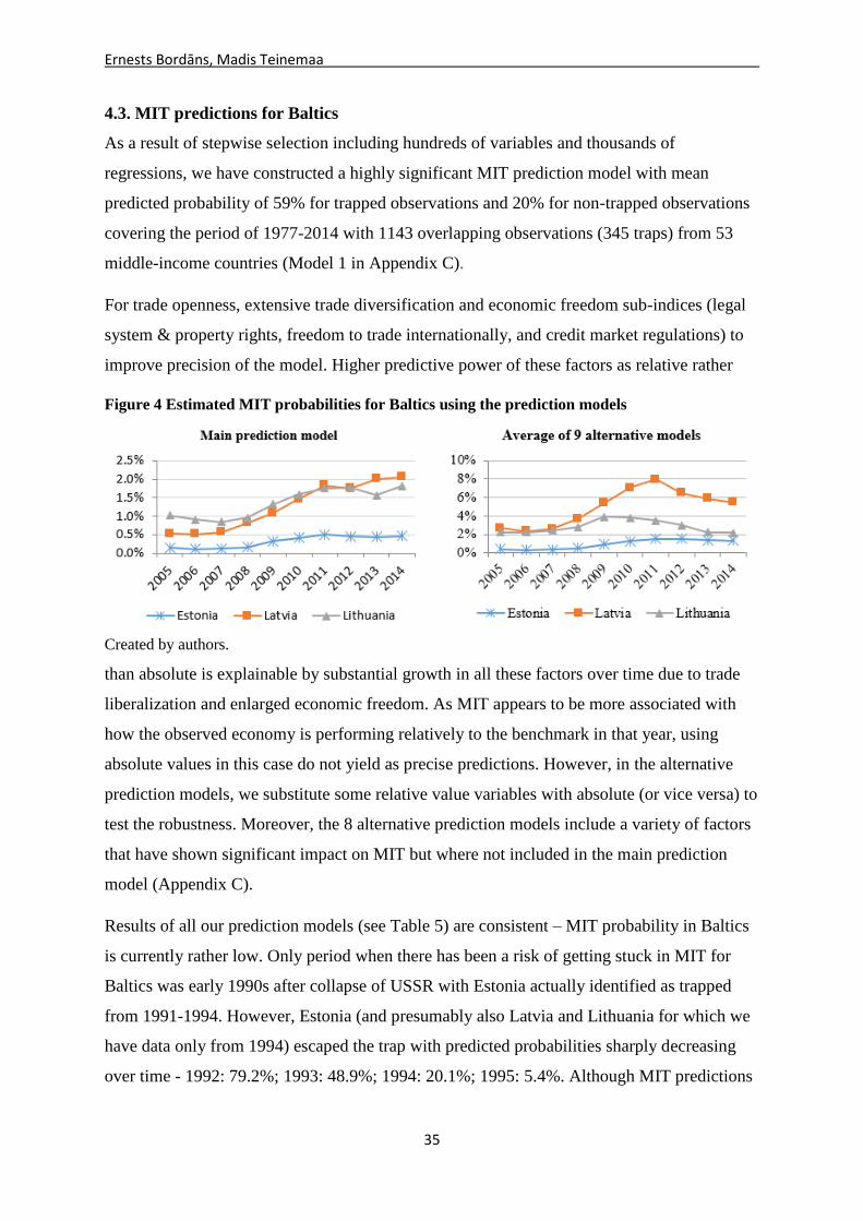
Ernests Bordāns, Madis Teinemaa
35
4.3. MIT predictions for Baltics
As a result of stepwise selection including hundreds of variables and thousands of
regressions, we have constructed a highly significant MIT prediction model with mean
predicted probability of 59% for trapped observations and 20% for non-trapped observations
covering the period of 1977-2014 with 1143 overlapping observations (345 traps) from 53
middle-income countries (Model 1 in Appendix C).
For trade openness, extensive trade diversification and economic freedom sub-indices (legal
system & property rights, freedom to trade internationally, and credit market regulations) to
improve precision of the model. Higher predictive power of these factors as relative rather
than absolute is explainable by substantial growth in all these factors over time due to trade
liberalization and enlarged economic freedom. As MIT appears to be more associated with
how the observed economy is performing relatively to the benchmark in that year, using
absolute values in this case do not yield as precise predictions. However, in the alternative
prediction models, we substitute some relative value variables with absolute (or vice versa) to
test the robustness. Moreover, the 8 alternative prediction models include a variety of factors
that have shown significant impact on MIT but where not included in the main prediction
model (Appendix C).
Results of all our prediction models (see Table 5) are consistent – MIT probability in Baltics
is currently rather low. Only period when there has been a risk of getting stuck in MIT for
Baltics was early 1990s after collapse of USSR with Estonia actually identified as trapped
from 1991-1994. However, Estonia (and presumably also Latvia and Lithuania for which we
have data only from 1994) escaped the trap with predicted probabilities sharply decreasing
over time - 1992: 79.2%; 1993: 48.9%; 1994: 20.1%; 1995: 5.4%. Although MIT predictions
Figure 4 Estimated MIT probabilities for Baltics using the prediction models
Created by authors.

Ernests Bordāns, Madis Teinemaa
36
have somewhat worsened since 2007 (see Figure 4), probabilities for Baltic countries remain
low in 2014 (Estonia: 0.46%, Latvia: 2.1%, Lithuania: 1.8%) compared to mean prediction
for middle-income countries (31.6%). To verify that low MIT predictions are not caused by
having too wide selection of countries in our dataset, we test robustness using more narrow
income range (30%-50% of US). Findings are consistent as MIT predictions for Baltics
remain at very low level (results available upon request).
Table 5 MIT prediction results with different model specifications (Model 1=the main prediction model)
Created by the authors.
Model 1 Model 2 Model 3 Model 4 Model 5 Model 6 Model 7 Model 8 Model 9
# variables 14 8 12 12 9 11 7 10 9
Estonia 0.46% 4.00% 0.92% 0.85% 2.81% 0.00% 1.22% 1.00% 0.74%
Latvia 2.06% 6.02% 4.50% 4.37% 8.31% 0.09% 2.56% 13.06% 8.41%
Lithuania 1.82% 4.71% 1.66% 2.49% 4.23% 0.00% 2.15% 1.77% 0.76%
Mean prediction for trapped obs. 58.68% 43.63% 51.32% 54.61% 42.14% 54.09% 37.26% 41.71% 39.63%
Mean prediction 31.63% 28.90% 29.52% 30.21% 26.47% 20.83% 22.19% 20.31% 19.54%
Mean prediction for non-trapped obs. 20.03% 22.77% 20.30% 20.13% 19.99% 10.62% 16.86% 13.82% 13.67%
# observations 1143 1420 1078 1096 1564 471 768 583 578
# traps 345 419 322 322 459 112 202 137 132
# countries 53 60 49 50 61 35 53 42 41
Beginning of period (year) 1977 1967 1977 1977 1967 1993 1993 1993 1993
Chi2 132.05 139.66 113.47 117.18 154.64 37.03 56 39.21 34.59

Ernests Bordāns, Madis Teinemaa
37
Italy, Greece, Spain, Cyprus and Portugal have the highest predicted MIT probabilities in
Europe (see Table 6) and are all identified as trapped (see Appendix B). Interestingly, our
prediction model would have indicated structural problems in these countries long before the
breakout of the European debt crisis (Figure 5). Structural reforms addressing poor
governance that followed bailout and intervention by IMF have lowered MIT probabilities in
Greece and significantly improved situation in Portugal (drop in MIT probability from 60.2%
in 2010 to 23.3% in 2014).
Meanwhile, Italy that has faced income divergence from wealthier European countries and
USA (and has fallen back to middle-income in 2010) has not been able to enforce structural
reforms and remains trapped with a small decline in prediction caused by decreasing GDP per
capita and income relative to trading partners. However, severe problems such as decreasing
enrolment in tertiary education, low and declining investment as % of GDP together with
rather high price level of capital and very low FDI net inflows are the actual causes behind
such high MIT prediction. Italy is an intriguing example, because it shows that the problem is
not merely about the middle income level and Baltic countries will have to keep up with
reforms and stay competitive also after reaching high-income.
Country MIT prob.
Italy 89.30%
Greece 79.06%
Spain 65.95%
Cyprus 23.82%
Portugal 23.20%
Poland 16.26%
Slovenia 9.23%
Croatia 8.67%
Slovakia 4.77%
Czech Republic 3.85%
Latvia 2.06%
Hungary 1.96%
Lithuania 1.82%
Bulgaria 1.12%
Estonia 0.46%
Romania 0.45%
0%
20%
40%
60%
80%
100%
2005 2006 2007 2008 2009 2010 2011 2012 2013 2014
Italy Greece
Spain MIT
MEAN Cyprus
Portugal NMIT
Poland Slovenia
Figure 5 Predicted MIT probabilities for Europe (2005-
2014)
Table 6 Predicted MIT
probabilities for Europe
(2014)
Created by the authors. Created by the authors.
Ernests Bordāns, Madis Teinemaa
38
Appendix F shows what have been the MIT predictions since 1977; and it is clearly
noticeable that predicted MIT probabilities in Europe are currently relatively low compared
to the rest of the world.
5. Discussion of Results
Analysis of results provided the reader with an answer to our first research question by
clearly outlining all observations of MITs historically and currently; as well as some
characteristics and frequency of MIT. In this section we move on to discuss how stable are
the predicted probabilities for Baltic countries facing the MIT, whether the Baltic economies
can be considered to be trapped according to other researchers’ offered MIT definitions and
which factors we consider to be possessing the highest risks specifically for the Baltics.
5.1 Predicted probability for the Baltic States
We test the sensitivity of MIT predictions for Baltic economies by adjusting variables that we
consider to be possible to influence by government policies. In positive development scenario
“HIC” these factors are raised to the level of high-income countries. In negative scenario
“MIC” we equalize all adjustable factors with an average level of middle-income countries.
Besides providing us with additional robustness check for MIT predictions, it also allows us
to analyse the impact of potential catch up or degeneration caused by unsuccessful policies as
well as identify factors with largest impact on Baltic economies. When making adjustments,
we assume that policy makers have a direct influence over quality of institutions, business
environment, tax policy, as well as enrolment rates in tertiary education (e.g. by providing
free higher education and equal opportunity for everyone to continue their studies through
scholarships). At the same time, we believe that Baltic governments do not have direct
influence over inflation (mostly affected by ECB), tariffs, trade openness (being part of EU
and WTO), price level of capital stock, export diversification, and external factors such as
current account balance, GDP per capita and relative trading partners’ wealth. Full list of
variables that we adjust and the extent of adjustment are reported in Appendix G. As can be
noted, negative adjustments in scenario “MIC” are substantial (considerably larger than
positive adjustments in scenario “HIC”) as all Baltic economies are currently much better
positioned with regard to these factors when compared to typical middle-income country.
In scenario “HIC”, results indicate that Estonia would not benefit from catching-up with
high-income countries (in certain factors) as much as Latvia and Lithuania, reflecting already
better institutions in Estonia (see Appendix H), however, it is more sensitive to “MIC”
scenario - on average the MIT probability for Estonia increases from 1.3% to 6.8%; whereas,

Ernests Bordāns, Madis Teinemaa
39
for Lithuania - from 2.2% to 5.2%. Nevertheless, it is still much below the mean predicted
probability of non-trapped observations under all model specifications.
Although deterioration of factors affected by government policies result with higher MIT
probabilities, the predictions for Baltics still remain very low (in the main model EE: 2.7%,
LV: 4%, LT: 3.4%) in comparison to mean prediction for actually trapped economies (58.7%
in the main model, 47% on average). Nonetheless, in some specifications MIT probability
increase can be substantial (e.g. from 8.4% to 25.7% for Latvia in Model 9).
After examining the underlying values of each factor for the Baltics and taking into account
which variables are always kept unchanged, we identify that MIT predictions for Baltic
economies are most exposed to changes in governance indicators (control of corruption,
government effectiveness, voice and accountability), income inequality, and legal system and
property rights. Moreover, we find that Latvia can reduce its highest predicted MIT
probability in Model 8 from 13.1% to 1.6% by reducing income inequality and corruption to
the mean level of high-income countries (GINI index from 35.6 to 31.1 and control of
corruption index from 0.2 to 1.8 (this index has values ranging from -2.5 to 2.5)).
After performing a robustness check by comparing MIT predictions for Baltics with other
European countries, using 8 alternative models covering different economic factors and time
periods (starting from 1967, 1977 or 1993 - depending on data availability), and adjusting
factors that can be affected by policy makers accordingly to a positive and a negative
development scenario, we conclude that there is robust evidence that none of the Baltic
countries is currently threatened by MIT. All Baltic economies are fundamentally in much
healthier condition than it would be expected from a typical middle-income country (and
current economic growth of the Baltic States ascertains that). However, MIT probabilities can
be further decreased by decreasing corruption (especially in Latvia), income inequality and
improving institutions (particularly public institutions in Latvia and Lithuania). Provided that
economic policy makers make no drastic reversals and consider following proposed
recommendations, we expect to see further convergence with the EU average income levels.
5.2. Performance of the Baltics in the context of previous literature MIT definitions
We have provided our argumentation for why in our opinion none of the existing MIT
definitions in the literature have the potential to successfully identify middle income traps.

Ernests Bordāns, Madis Teinemaa
40
However, for the benefit of the reader, we look at whether the existing definitions identify
any of the Baltic States to be trapped10.
Firstly, we must acknowledge that according to the middle income level classifications
offered by the World Bank, Aiyar et.al. (2012) and Robertson et.al. (2013) all three Baltic
States have already graduated from the middle income level and are now (as of 2014)
classified as high income countries (upper thresholds of middle income level proposed by
these sources are - 12,736$ (GNI per capita at 2014$), 15,000$ (GDP per capita at PPP
2005$) and 8-36% of the USA’s GDP per capita at PPP respectively11. Hence, according to
these authors, Baltics have already avoided the MIT. (Except, in 2014 Latvia was still at 35%
of the USA’s income level).
GDP per capita data for the Baltics is only available since 1993 (for Estonia – since 1990)12,
when they entered the dataset as middle income countries already. Hence, we do not know
exactly how long Baltics have been at middle income level, and we cannot compare their
time spent as middle income countries to the benchmarks offered by Felipe et.al. (2012), who
argued that if country’s income level is between 2,988$ and 17,557$ (2005$ at PPP) for
longer than 42 years, the country is trapped. However, he specified that there is also “upper
MIT”, where country is trapped if its income level is between 10,833$ and 17,557$ for longer
than 14 years. Both, Estonia and Lithuania was at this income level for 12 years before
graduating in 2011 and 2014 respectively. However, according to Felipe et.al. (2012) Latvia
still must grow with at least 3.5% per year in order to avoid the “upper MIT”, which apart
from years 2008-2010 it has achieved.
Robertson et.al (2013) conditions that a country is trapped if in the long term the difference
between certain country’s log income and the USA log income is stationary. As long as the
data is available, this is not the case for the Baltics, because since 1994, GDP per capita of
Estonia, Latvia and Lithuania relatively to the USA has gradually increased by around 25, 17
and 18 pp respectively.
Lastly, Eichengreen et.al. (2014) defines MIT as the moment when historical 7-year (t-7)
average growth has been considerably higher (by at least 2 pp) than future 7-year (t+7)
10 None of the existing papers have identified any of the Baltic States to be in the MIT; however, they have not used GDP per capita data until 2014 and some of the papers exclude the Baltics from their data sample. 11 All GDP per capita figures for estimates are acquired from Penn World Tables 7.1 database until 2010, and extrapolated till 2014 using the GDP per capita at PPP growth rates from the World Bank WDI database. 12 Penn World Tables 7.1 database.

Ernests Bordāns, Madis Teinemaa
41
growth rate (conditioning that country’s 7-year average (t-7) growth before was at least 3.5%
p.a. According to Eichengreen et.al., all three Baltic States were trapped between 2002 and
2007 (Lithuania – since 2003) (we cannot say anything about the situation after 2007 because
we need to know growth rates from 2015 onwards to calculate future (t+7) average growth
rate). Such proposition is rather controversial, because firstly, it is hard to comprehend why
should economies be considered to be trapped when they are still growing more than 7% p.a.,
as was the case in the Baltics between 2002 and 2007; and secondly, since 2010 the 7-year
historical average growth of Baltics economies has been below 3.5%; hence, according to
Eichengreen et.al. (2014) they cannot classify to be experiencing MIT. To our mind, the case
of the Baltics ascertains that Eichengreen et.al. (2014) definition is flawed.
To sum up, none of the existing MIT definitions clearly suggest that the Baltics are caught in
the MIT as of 2014.
5.3. Discussion of key determinants of MIT: relevance for the Baltics
5.3.1. Income level
Joining the EU catalysed the development of Baltic countries by larger capital inflow, import
of innovations and crucially - implementation of institutional and economic reforms (e.g. in
order to fulfil the Copenhagen criteria) (Kasjanovs and Meļihovs, 2011). Baltic countries
have caught up with their trading partners significantly since 2000 (Lithuania and Estonia
from around 45% to almost 70%; and Latvia from around 34% to 62% in 2014 (authors’
estimates based on IMF DOTS). This development might be attributed to club convergence
(Islam, 2003). Kasjanovs (2015) has speculated that Latvia may fall into MIT in the medium
term upon reaching approximately 75% of the EU average. We test this hypothesis with our
main prediction model by virtually increasing GDP per capita of Latvia by 25%, and the
income level relative to its trading partners’ to 75%. The estimated probability for Latvia in
such case is 5.4%. An increase from 2.1% to 5.4% is considerable; however, it is still
relatively small compared to other middle income countries. Nevertheless, it also indicates
that as the Baltic economies grow, the probability of getting trapped will increase inevitably,
and the only way how policy makers can avoid increasing probability of getting trapped is by
improving factors that they can influence with consistent structural reforms.
5.3.2. Macro stability
We have found macroeconomic stability to have a significant and robust effect on decreasing
the probability of MIT. Price stability is necessary especially for middle income countries for
easier attraction of investments to improve productivity and reach high-income level (Sala-i-
Ernests Bordāns, Madis Teinemaa
42
Martin, 1997) (Fischer, 1993). Moreover, price stability is also closely associated with the
price level of capital stock, that must be maintained low to assure a more favourable
environment for investments.
Furthermore, unsustainably high budget deficits have caused several EU countries to face
prolonged debt crisis; moreover, Fischer (1993) suggests that macroeconomic uncertainty
caused by budget deficit has a negative impact on productivity growth (through lower
efficiency of price mechanism) and adverse effect on investment rates. Fortunately, the Baltic
States are among very few European countries to fulfil the Maastricht criteria and have a low
budget deficit, and our findings recommend them to stay on this path.
5.3.3. Competitiveness
Baltic policy makers must keep a close eye on labour costs that have continued to increase
steadily in the Baltic States since a drop in 2009. Relatedly, the compensation of employees
as a share of GDP has increased by around 4.5 pp in Latvia and Estonia since 2013 (though
still below the peak in 2008), which indicates that compensation is increasing more than
productivity, and that has an adverse impact on competitiveness (Eurostat, 2015).
Losing competitiveness can turn out to be the prevailing factor for trapping the Baltic States,
given that REER level in the Baltics has been recently increasing considerably faster than in
most other EMU countries (Bruegel, 2015). Our finding on the effect of REER differs from
Eichengreen et al. (2014) who argued that undervaluation makes countries less incentivized
to initiate reforms for long term growth. However, we believe that high REER has an adverse
impact on growth, as it implies lack of competitiveness and is associated with shrinking
exports (Rodrik, 2008). After joining the EMU, the only way how Baltic countries can
increase their competitiveness when trading with Eurozone is by a decrease in real factor
prices or increase in productivity, as no currency adjustments are possible. When trading with
countries outside Eurozone, currency rates may fluctuate, but it happens outside direct control
of Baltic governments and central banks. Such situation has pushed several European
countries (e.g. Portugal, Greece) into having overvalued currencies (De Grauwe, 2006), and
as Eichengreen (2010) suggests, the Baltic countries might experience a similar scenario of
large capital inflows and economic growth followed by overvalued currency and economic
stagnation, in case they do not control their spending at all times.
Furthermore, Baltic States are significantly lagging behind high income countries in terms of
innovations and business sophistication (as shown by Global Competitiveness Report).
Ernests Bordāns, Madis Teinemaa
43
However, we find related factors to have a significant impact on decreasing the probability of
MIT. Moreover, literature suggests that innovations are particularly important for a country to
advance to high income level and reach the “4th stage” of economic development, where
country can lead innovations on global scale (Ohno, 2009). Unfortunately for Baltics, lack of
innovation and business sophistication can jeopardize their transition to high income.
5.3.4. Economic structure
As mentioned, investment rate has one of the most significant and robust negative impact on
the probability of MIT. Previous empirical economic growth research has provided rather
strong results for relationship between investments share and GDP growth (De Long and
Summers, 1991) (Sala-i-Martin, 1997). Investments are important for countries with a risk of
being caught in the MIT, because shift from labour-intensive to more technology-intensive
industries cannot happen without capital investments. Staehr (2015) has claimed that
relatively large investment rates in the Baltics indicate that marginal returns of capital are still
fairly high in this region. Nevertheless, investment rates can also be influenced by
government policy actions (can be one of the reasons why Estonia has higher investment
rates) e.g. by stronger rule of law, stable macroeconomic environment, tax incentives etc.
Moreover, the significant and robust impact of government size on the probability of MIT
suggests that improving the private sector activity at middle income level is more important
and yields higher marginal returns than high government expenditure (Aiyar et.al. 2013).
Estonia has been the leader in terms of both domestic and foreign direct investment activity
in the Baltics, and that may be attributed to its outperformance in institutions, e.g. economic
freedom. Notably, success of Finland, South Korea and Ireland was also chiefly driven by
FDI (Foxley and Sossdorf, 2011), and hopefully soon enough we will be able to add (at least)
Estonia to the list of countries that have escaped the MIT by attracting high-technology FDI.
5.3.5. Human capital
We find higher tertiary education enrolment to be consistently associated with lower MIT
probability. This is in line with previous research as improved human capital has been
emphasised as important factor to avoid MIT by various authors (Liu et al. 2013) (Egawa,
2013) (Staehr, 2015) (Agenor et.al, 2015). Kharas et.al. (2011) points out that development of
tertiary education is one of the key differences between rapidly growing East Asia and
trapped Latin America.
Availability and quality of tertiary education should be one of the key concerns for policy
makers in the Baltics if they wish to avoid the MIT. Not only educated labour force is crucial
Ernests Bordāns, Madis Teinemaa
44
for innovations and higher productivity, but improved education availability may also
decrease income inequality (which is one of the problematic factors for the Baltic States on
its own) (Liu, Luo, Rozelle, Yi and Zhang, 2013) (Egawa, 2013).
Education has been a hot topic in the Baltics. While higher education enrolment rates are
relatively high, the education quality is often challenged. IMF (2015) and OECD (2015)
explain that Latvia and Lithuania still lack high-skilled workforce which is hard to obtain
without improving the weak state of vocational education.
5.3.6. Income inequality
We find that income inequality has a significant and positive impact on the probability of
MIT. Already the seminal papers on MIT identify the crucial role that middle class ought to
play in middle income countries advancement to high income (Kharas et.al. 2011) (Berg et.al.
2012). They explain that growth in the domestic demand largely depends on the consumption
of middle class, as countries cannot rely on ever increasing net exports.
Unfortunately, Latvia and Lithuania are among the most unequal countries in the EU, and
OECD (2015) has explicitly pointed out that Latvia’s and Lithuania’s inequality problems
can be a cause for further worsening skills mismatch, worse health of the society and
generally less sustainable development. Hence, we would recommend Baltic policy makers to
address this painful issue by e.g. reforming the educational system to decrease existing skill
mismatches.
5.3.7. Public sector performance
Arguably, strong governance is one of the most important factors for avoiding the MIT
because transition to high income requires decisive policy and structural reforms. South
European countries (e.g. Italy) have shown that delaying reforms can even drag a high-
income country back into middle income level. Baltic States have become notorious for
structural reforms (drastic internal devaluation) pulled out during the crisis. However,
implementing reforms during “peace times” when they can be targeted at maintaining long
term growth, not fighting fire, comes harder; and weak governance may be one of the
reasons.
Particularly Latvia and Lithuania are ranking rather poorly by the overall quality of their
public institutions in the Global Competitiveness Report (Lithuania – 53rd, Latvia – 50th).
Fish rots from its head, and metaphorically we see this as one of the key risks facing
Lithuania and Latvia. Not only because weak institutions have an adverse impact on the

Ernests Bordāns, Madis Teinemaa
45
performance today (higher corruption, lower tax collection, worse investment environment,
higher wastefulness of funds etc.) but chiefly because these countries can be trapped in a
vicious cycle where lack of decisive structural reforms weakens the governance quality even
further. Latvia and Lithuania rank 81st and 92nd respectively in terms of wastefulness of
government spending, next to Tanzania, Cameroon and Russia. Overall public-sector
performance is also at rather low levels – Latvia is ranked 74th and Lithuania – 76th. Delayed
public healthcare and education system reforms in Latvia present the indecisiveness of
government even in sectors that are harming society’s well-being today (not even mentioning
lack of long-term strategy). Such weak rankings in factors that we find to have a significant
and robust impact on increasing the probability of MIT (e.g. wastefulness of spending) is
even more alarming.
Moreover, our findings on legal system’s impact on the probability of MIT are in line with
previous literature claiming that property rights and rule of law fosters countries convergence
with high income countries (Knack and Keefer, 1995). Improvements in judicial system
require major structural reforms but Latvia and Lithuania are struggling. IMF (2015)
recommends judiciary system reforms as one of the key structural changes for Latvia, as
extremely long trials and stagnating insolvency process reform are some examples of how
inefficient system undermine country’s business environment and international image.
5.3.8. Corruption
Sadly, we must also discuss the dramatic impact that corruption in the Baltics can have on
increasing the probability of MIT. As outlined previously, different corruption proxies are
found to have a robust and significant impact on the MIT. Corruption can drag countries into
the MIT by ruining the efficiency of resource allocation, ruining business environment and
country’s reputation in the eyes of international investors through unfair government tenders,
corrupt CEOs of state owned enterprises, vested interests of political party sponsors and
unfair court judgments. OECD’s continuous indications at problems with Latvia’s anti-
corruption policies (being one of the reasons for not getting accepted at OECD) is a good
example of how governance problems undermine country’s prospects for development
(OECD, 2015). Unfortunately, in almost all corruption proxies the Baltic countries are still
significantly lagging behind high-income countries. It has been shown by previous
researchers that weak public institutions are often the main cause for higher levels of
corruption (Abed and Davoodi, 2000).

Ernests Bordāns, Madis Teinemaa
46
6. Conclusions
After seeing so many economists referring to the Baltic States in the context of possible
middle income trap, we tested the appropriateness of such speculations. This paper has
supplemented the existing literature in numerous ways. Firstly, we propose and apply our
own definition of middle income trap which captures all characteristics of a good MIT
definition by using country-specific benchmarks that successfully identify economic
slowdowns that we believe can be characterized as middle income traps. By using the most
extensive dataset that includes all factors that previous literature has mentioned to have a
significant impact on the probability of middle income trap we, firstly, assess which factors
have a significant and robust impact on the probability of MIT and, secondly, construct a
multivariate panel data logit prediction model and quantitatively estimate the probability of
each of the Baltic State to be facing middle income trap.
We answered three research questions:
1) Which countries have historically been or currently are caught in the MIT?
We find that 32% of middle income countries have historically been caught in a middle
income trap, with the highest frequency of traps occurring in Latin America. None of the
Baltic States are currently trapped; however, among European countries Italy, Greece,
Cyprus, Portugal and Spain are currently trapped. Importantly, our model has shown
increased MIT probabilities for these countries well before a trap has actually occurred.
2) What is the current probability of Baltic countries facing the MIT and which Baltic
country is most likely to get trapped?
By employing numerous prediction models we find robust evidence that the probability of
Baltic countries currently facing MIT is rather low (below 10%) when compared to global
average. Moreover, we test our prediction models by adjusting some of the factor values for
the Baltic States and see that no significant change in the predicted probability of MIT can be
expected in the nearest future. Moreover, we find that the lowest probability of getting
trapped exists for Estonia; whereas, the highest – for Latvia.
Additionally, we show that according to all MIT definitions offered in previous literature,
Baltic countries cannot be considered to be in the MIT.
3)Which exogenous factors possess the highest risk for increasing the probability of MIT
occurrence in the Baltic States?
Ernests Bordāns, Madis Teinemaa
47
We find that the recipe for avoiding middle income trap consists of strong public sector with
abilities to implement structural reforms, low corruption, income equality, business friendly
and free economy, strong institutions, sound macroeconomic environment with low inflation,
advanced and equally available tertiary education, business-friendly regulations and taxation,
highly sophisticated yet diversified exports, and economic structure with small government
and large share of investments.
In addition to bringing attention to over 100 economic indicators that have significant impact
over MIT likelihood; we have busted the myth of middle income trap in Baltics.
Nevertheless, with increasing absolute income level and income level relatively to trading
partners, the probability of Baltic States facing the trap will increase; hence, continuous
structural reforms are necessary in order to maintain the MIT probability low also in the
future.

Ernests Bordāns, Madis Teinemaa
48
7. Reference list
Abed, M. G. T., & Davoodi, M. H. R. (2000). Corruption, Structural Reforms, and Economic
Performance in the Transition Economies (No. 0-132). International Monetary Fund.
Aiyar, M. S., Duval, M. R. A., Puy, M. D., Wu, M. Y., & Zhang, M. L. (2013). Growth
slowdowns and the middle-income trap (No. 13-71). International Monetary Fund.
Arora, V., & Vamvakidis, A. (2005). How much do trading partners matter for economic
growth? IMF staff papers, 24-40.
Aten, B., Heston, A., Summers, R., (2012) Penn World Table Version 7.1 Center for
International Comparisons of Production, Income and Prices. University of
Pennsylvania.
BBVA Research. (2015). Global Economic Outlook. First quarter 2015.
Retrieved March 2, 2016, from https://www.bbvaresearch.com/wp-
content/uploads/2015/02/Global_Economic_Outlook_1Q15-Cap3.pdf
Berg, A., Ostry, J. D., & Zettelmeyer, J. (2012). What makes growth sustained?. Journal of
Development Economics, 98(2), 149-166.
Bursac, Z., Gauss, C. H., Williams, D. K., & Hosmer, D. W. (2008). Purposeful selection of
variables in logistic regression. Source code for biology and medicine, 3(1), 1.
Bruegel. (2015). Real effective exchange rates for 178 countries: a new database [Data file].
Retrieved January 5, 2016, from http://bruegel.org/publications/datasets/real-
effective-exchange-rates-for-178-countries-a-new-database/
Cimoli, M., & Correa, N. (2002). Trade openness and technological gaps in Latin America: a
low growth trap. Laboratory of Economics and Management Working Paper Series
No14, Pisa.
Cogley, T., & Nason, J. M. (1995). Effects of the Hodrick-Prescott filter on trend and
difference stationary time series Implications for business cycle research. Journal of
Economic Dynamics and control, 19(1), 253-278.
De Grauwe, P. (2006). What Have we Learnt about Monetary Integration since the
Maastricht Treaty?*. JCMS: Journal of Common Market Studies,44(4), 711-730
De Long, J. B., & Summers, L. H. (1990). Equipment investment and economic growth (No.
w3515). National Bureau of Economic Research.
Durlauf, S. N., & Quah, D. T. (1999). The new empirics of economic growth. Handbook of
macroeconomics, 1, 235-308.
Egawa, A. (2013). Will income inequality cause a middle-income trap in Asia (No. 797).
Ernests Bordāns, Madis Teinemaa
49
Eichengreen, B. (2010). The breakup of the euro area. In Europe and the Euro (pp. 11-51).
University of Chicago Press.
Eichengreen, B., Park, D., & Shin, K. (2014). Growth slowdowns redux. Japan and the
World Economy, 32, 65-84.
Eurostat Statistics Database. (n.d.). Eurostat. Retrieved 06.12.2015 from
http://epp.eurostat.ec.europa.eu/portal/page/portal/statistics/search_database
Felipe, J., Abdon, A., & Kumar, U. (2012). Tracking the middle-income trap: What is it, who
is in it, and why?. Levy Economics Institute, Working Paper, (715).
Fischer, S. (1993). The role of macroeconomic factors in growth. Journal of monetary
economics, 32(3), 485-512.
Foxley, A., & Sossdorf, F. (2011). Making the transition: From middle-income to advanced
economies. Carnegie Endowment for International Peace.
Gill, I. S., Kharas, H. J., & Bhattasali, D. (2007). An East Asian renaissance: ideas for
economic growth. World Bank Publications.
Gwartney, J., Lawson, R., & Hall, J. (2015). Economic freedom of the world 2015 annual
report. The Fraser Institute.
Han, X., & Wei, S. J. (2015). Re-examining the Middle Income Trap Hypothesis: What to
Reject and What to Revive?.
Hansen, M. (2013, July 23). Of Latvian Growth and convergence [Blog post]. Retrieved from
http://www.ir.lv:889/2013/7/23/of-latvian-growth-and-convergence
Hausman, J., & McFadden, D. (1984). Specification tests for the multinomial logit model.
Econometrica: Journal of the Econometric Society, 1219-1240.
Hausmann, R., & Klinger, B. (2006). Structural transformation and patterns of comparative
advantage in the product space.
Hausmann, R., Hidalgo, C. A., Bustos, S., Coscia, M., Simoes, A., & Yildirim, M. A. (2014).
The atlas of economic complexity: Mapping paths to prosperity. Mit Press.
Hausmann, R., Pritchett, L., & Rodrik, D. (2005). Growth accelerations. Journal of Economic
Growth, 10(4), 303-329.
Hoetker, G. (2007). The use of logit and probit models in strategic management research:
Critical issues. Strategic Management Journal, 28(4), 331-343.
Hosmer Jr, D. W., Lemeshow, S., & Sturdivant, R. X. (2000). Model‐building strategies and
methods for logistic regression. Applied Logistic Regression, Third Edition, 89-151.’

Ernests Bordāns, Madis Teinemaa
50
International Monetary Fund. (2014) “Sustaining Long-Run Growth and Macroeconomic
Stability in Low-Income Countries: The Role of Structural Transformation and
Diversification.” IMF Policy Paper, Washington, March.
International Monetary Fund. (2015). Republic of Latvia : Staff Report for the 2015 Article IV
Consultation. Washington, D.C.
International Monetary Fund. (2015). Republic of Latvia: Selected Issues. Retrieved from
http://www.imf.org/external/pubs/ft/scr/2015/cr15111.pdf
Islam, N. (1995). Growth empirics: a panel data approach. The Quarterly Journal of
Economics, 1127-1170.
Islam, N. (2003). What have we learnt from the convergence debate?. Journal of economic
surveys, 17(3), 309-362.
Kasjanovs, I. (2015). Is part of the Latvian economy already in the middle-income trap?.
World Economics, 16(1), 58-69.
Kharas, H., & Kohli, H. (2011). What is the middle income trap, why do countries fall into it,
and how can it be avoided?. Global Journal of Emerging Market Economies, 3(3),
281-289.
Knack, S., & Keefer, P. (1995). Institutions and economic performance: Cross-country tests
using alternative institutional indicators.
Levine, R. (2001). International financial liberalization and economic growth.Review of
international Economics, 9(4), 688-702.
Levine, R., & Renelt, D. (1991). Cross-country studies of growth and policy: methodological,
conceptual, and statistical problems (Vol. 608). World Bank Publications.
Levine, R., & Renelt, D. (1992). A sensitivity analysis of cross-country growth regressions.
The American economic review, 942-963.
Levine, R., & Zervos, S. J. (1993). What we have learned about policy and growth from
cross-country regressions?. The American Economic Review,83(2), 426-430.
Meļihovs, A., & Kasjanovs, I. (2011). The convergence processes in Europe and Latvia (No.
2011/01). Latvijas Banka.
North, D. C. (1990). Institutions, institutional change and economic performance. Cambridge
university press.
OECD Publishing. (2015). OECD Economic Surveys: Latvia 2015. OECD Pub.
Ohno, K. (2009). Avoiding the middle-income trap: renovating industrial policy formulation
in Vietnam. ASEAN Economic Bulletin, 26(1), 25-43.
Ernests Bordāns, Madis Teinemaa
51
Peng, C. Y. J., Lee, K. L., & Ingersoll, G. M. (2002). An introduction to logistic regression
analysis and reporting. The Journal of Educational Research, 96(1), 3-14.
Quah, D. T. (1996). Empirics for economic growth and convergence. European economic
review, 40(6), 1353-1375.
Rodrik, D. (2008). The real exchange rate and economic growth. Brookings papers on
economic activity, 2008(2), 365-412.
Sala-i-Martin, X. X. (1996). Regional cohesion: evidence and theories of regional growth and
convergence. European Economic Review, 40(6), 1325-1352.
Sala-i-Martin, X. X. (1996). The classical approach to convergence analysis.The economic
journal, 1019-1036.
Sala-i-Martin, X. X. (1997). I just ran four million regressions (No. w6252). National Bureau
of Economic Research.
Staehr, K. (2015). Economic Growth and Convergence in the Baltic States: Caught in a
Middle-Income Trap?. Intereconomics, 50(5), 274-280.
Strašuna, L. (2015, July) General Government spending - how much and on what. Macro
Research: The Latvian Economy. Retreived from
https://www.swedbank.lv/files/analitiskie_materiali/menesa_apskats/The_Latvian_Ec
onomy_2015_07_EN.pdf
The World Bank Database (2014, March 7). Updated Income Classifications. Retrieved
November 20, 2015, from http://data.worldbank.org/news/2015-country-
classifications
Tho, T. V. (2013). The middle-income trap: Issues for members of the Association of
Southeast Asian nations. Asian Development Bank Institute Working Paper, 421.
Williams, R. (2012). Using the margins command to estimate and interpret adjusted
predictions and marginal effects. Stata Journal, 12(2), 308.
Williams., R. Marginal Effects for Continuous Variables. February, 2015. University of Notre
Dame. Retreive 06.02.2016 from:
https://www3.nd.edu/~rwilliam/stats3/Margins02.pdf
Woo, W. T. (2012). China meets the middle-income trap: the large potholes in the road to
catching-up. Journal of Chinese Economic and Business Studies,10(4), 313-336.
Ye, L., & Robertson, P. E. (2013). On the Existence of a Middle-Income Trap. Economics
Discussion Paper 13.12. University of Western Australia
Zhang, L., Yi, H., Luo, R., Liu, C., & Rozelle, S. (2013). The human capital roots of the
middle income trap: the case of China. Agricultural Economics,44(s1), 151-162.
Ernests Bordāns, Madis Teinemaa
52
8. Appendices
Appendix A. All middle income level countries identified between 1960 and 2014.
Appendix B. All Middle Income Traps identified between 1960 and 2014.
Nr
of
ob
s.
% t
rap
ped
Nr
of
ob
s.
% t
rap
ped
Nr
of
ob
s.
% t
rap
ped
Nr
of
ob
s.
% t
rap
ped
Albania 3 0% Turkey 55 27% Panama 49 12% Macedonia 23 48%Austria 11 0% Ukraine 7 29% Czech Rep 24 13% Guatemala 35 49%Belarus 13 0% Mexico 55 29% Singapore 31 13% New Zealand 32 50%China 3 0% Poland 44 30% Israel 55 15% Algeria 36 53%Finland 21 0% Portugal 55 31% Estonia 24 17% S. Africa 20 55%France 9 0% Spain 55 31% Slovenia 24 17% Jordan 16 56%Hong Kong 32 0% Romania 41 32% Mauritius 29 17% Peru 36 58%Japan 16 0% Ukraine 22 32% Serbia 17 18% Nicaragua 21 62%Korea, Rep. 39 0% Cyprus 55 33% Ireland 39 18% Eq. Guinea 12 67%Latvia 21 0% Russia 24 33% Slovakia 25 20% Jamaica 55 67%Lithuania 21 0% Suriname 44 34% Thailand 18 22% Venezuela 55 67%Malaysia 34 0% Chile 55 35% Italy 21 24% Argentina 51 69%Montenegro 5 0% Lebanon 43 40% Hungary 44 25% Ecuador 26 69%Tunisia 3 0% Iran 48 40% Colombia 53 26% Barbados 11 100%Dom. Rep. 41 2% Croatia 24 42% Bulgaria 37 27% Bolivia 11 100%Macao SAR 30 3% Uruguay 55 44% Brazil 55 27% Djibouti 4 100%Malta 44 9% Greece 55 45% Costa Rica 55 27% El Salvador 27 100%
Algeria 1961 - 1966 Estonia 1991 - 1994 Panama 1972 - 19721971 - 1973 Greece 1979 - 1995 1996 - 20001987 - 1995 2007 - 2014 Peru 1967 - 19682014 - 2014 Guatemala 1960 - 1963 1971 - 1971
Argentina 1960 - 1988 1979 - 1991 1974 - 19911997 - 2002 Hungary 1986 - 1996 Poland 1978 - 1990
Barbados 2004 - 2014 Iran 1978 - 1989 Portugal 1976 - 1977Bolivia 1960 - 1970 2008 - 2014 2000 - 2014Brazil 1980 - 1982 Ireland 1981 - 1987 Romania 1985 - 1997
1988 - 1990 Israel 1998 - 2005 Russia 1991 - 19981996 - 2004 Italy 2010 - 2014 Serbia 1995 - 1997
Bulgaria 1990 - 1999 Jamaica 1963 - 1968 Singapore 1961 - 1964Chile 1961 - 1977 1972 - 1982 Slovakia 1990 - 1994
1982 - 1983 1995 - 2014 Slovenia 2011 - 2014Colombia 1960 - 1966 Jordan 1966 - 1972 South Africa 1997 - 2000
1996 - 2002 1985 - 1986 2008 - 2014Costa Rica 1961 - 1965 Lebanon 1971 - 1976 Spain 1979 - 1984
1976 - 1985 1978 - 1979 2004 - 2014Croatia 1991 - 1995 1987 - 1990 Suriname 1986 - 2000
2010 - 2014 1997 - 2001 Thailand 1997 - 2000Cyprus 1960 - 1961 Macao SAR 1999 - 1999 Turkey 1960 - 1964
1971 - 1974 Macedonia 1991 - 2001 1977 - 19811997 - 2000 Malta 2001 - 2004 1997 - 20012007 - 2014 Mauritius 1960 - 1964 Ukraine 1994 - 1995
Czech Republic 1991 - 1991 Mexico 1983 - 1988 UK 1967 - 19731997 - 1998 1994 - 1996 Uruguay 1960 - 1971
Djibouti 1978 - 1981 2003 - 2004 1980 - 1985Dominican Rep. 1965 - 1965 2008 - 2010 1998 - 2003Ecuador 1960 - 1967 2013 - 2014 Venezuela, RB 1960 - 1968
1981 - 1990 New Zealand 1982 - 1984 1976 - 1987El Salvador 1960 - 1985 1986 - 1993 1995 - 2003
2014 - 2014 2003 - 2007 2008 - 2014Eq. Guinea 2007 - 2014 Nicaragua 1968 - 1980
Created by the authors.
Created by the authors.
Ernests Bordāns, Madis Teinemaa
53
Appendix C. Prediction models
Created by the authors.
Logit regressions Model 1 Model 2 Model 3 Model 4 Model 5 Model 6 Model 7 Model 8 Model 9
GDP per capita x1000 0.147** 0.313*** 0.131* 1.340*** 0.197***
Investment % of GDP -0.088*** -0.052*** -0.057** -0.035** -0.060**
Gov. % of GDP 0.135*** 0.215*** 0.155*** 0.115*** 0.202*** 0.801** 0.233*** 0.330*** 0.359***
(Relative) Trade openness -0.026*** -0.032*** -0.040*** -0.028*** -0.030***
(Relative) Freedom to trade internationally -0.014** -0.020*** -0.019***
(Relative) Legal System & Property Rights -0.016** -0.020*** -0.018** -0.013***
Tertiary edu.enrol. -0.047*** -0.029*** -0.031***
Foreign direct investment, net inflows (% of GDP) -0.086** -0.126**
Current Account -0.081*** -0.069** -0.059**
Price lev. of cap. stock 1.022* 1.802***
Inflation 0.007*** 0.009*** 0.008*** 0.075***
(Relative) Relative TP wealth 3.622*** 3.796*** 2.657* 3.568*** 5.551** 5.595**
(Relative) Extensive Margin 0.012***
(Relative) Credit market regulations -0.010*
Legal System & Property Rights -0.242**
Regulation -0.262**
Freedom to trade internationally -0.251***
(Relative) Tertiary edu.enrol. -0.009**
Consumption % of GDP -0.054**
(Relative) Price lev. of cap. stock 0.010**
Export Diversification 0.548** 0.367*
Economic Complexity -0.690* -0.684*
Trade openness -0.042*** -0.026***
(Relative) Sound Money -0.013***
(Relative) Exports % as of GDP -0.026***
TP growth -45.88***
Price of investment 0.116*** 0.032** 0.036**
Size of Government -1.424**
Protection of property rights -1.717**
Credit market regulations -1.504***
GINI index (World Bank estimate) 0.512*** 0.133** 0.138**
(Relative) Researchers in R&D (per million people) -0.002***
Tariff rate, applied, simple mean, all products (%) 0.822***
Cash surplus % of GDP -0.395*
Taxes on income, profits and capital gains (% of revenue) 0.059** 0.053* 0.063**
Taxes on goods and services (% of revenue) -0.090*** -0.057* -0.053*
Government Effectiveness (estimate) -1.793***
Control of Corruption (estimate) -1.030*
Lending interest rate 0.008**
Voice and Accountability (estimate) -1.330*
Interest rate spread (lending rate minus deposit rate, %) 0.025**
_cons 1.029 1.081 1.65 1.858 1.149 -37.49*** -2.600 -14.66*** -15.66***
Observations 1143 1420 1078 1096 1564 471 768 583 578
Source: Authors' calculations.
Model 1 is the main MIT prediction model.
* Statistically significant at the 10% level.
** Statistically significant at the 5% level.
*** Statistically significant at the 1% level.
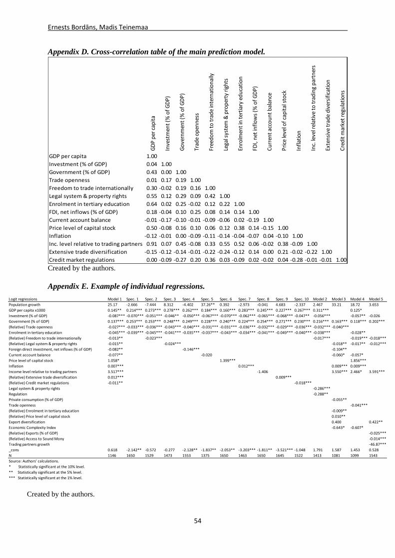
Ernests Bordāns, Madis Teinemaa
54
Appendix D. Cross-correlation table of the main prediction model.
Appendix E. Example of individual regressions.
GD
P p
er c
apit
a
Inve
stm
ent
(% o
f G
DP
)
Go
vern
men
t (%
of
GD
P)
Trad
e o
pen
nes
s
Free
do
m t
o t
rad
e in
tern
atio
nal
ly
Lega
l sys
tem
& p
rop
erty
rig
hts
Enro
lmen
t in
ter
tiar
y ed
uca
tio
n
FDI,
net
infl
ow
s (%
of
GD
P)
Cu
rren
t ac
cou
nt
bal
ance
Pri
ce le
vel o
f ca
pit
al s
tock
Infl
atio
n
Inc.
leve
l rel
ativ
e to
tra
din
g p
artn
ers
Exte
nsi
ve t
rad
e d
iver
sifi
cati
on
Cre
dit
mar
ket
regu
lati
on
s
GDP per capita 1.00
Investment (% of GDP) 0.04 1.00
Government (% of GDP) 0.43 0.00 1.00
Trade openness 0.01 0.17 0.19 1.00
Freedom to trade internationally 0.30 -0.02 0.19 0.16 1.00
Legal system & property rights 0.55 0.12 0.29 0.09 0.42 1.00
Enrolment in tertiary education 0.64 0.02 0.25 -0.02 0.12 0.22 1.00
FDI, net inflows (% of GDP) 0.18 -0.04 0.10 0.25 0.08 0.14 0.14 1.00
Current account balance -0.01 -0.17 -0.10 -0.01 -0.09 -0.06 0.02 -0.19 1.00
Price level of capital stock 0.50 -0.08 0.16 0.10 0.06 0.12 0.38 0.14 -0.15 1.00
Inflation -0.12 -0.01 0.00 -0.09 -0.11 -0.14 -0.04 -0.07 0.04 -0.10 1.00
Inc. level relative to trading partners 0.91 0.07 0.45 -0.08 0.33 0.55 0.52 0.06 -0.02 0.38 -0.09 1.00
Extensive trade diversification -0.15 -0.12 -0.14 -0.01 -0.22 -0.24 -0.12 0.14 0.00 0.21 -0.02 -0.22 1.00
Credit market regulations 0.00 -0.09 -0.27 0.20 0.36 0.03 -0.09 0.02 -0.02 0.04 -0.28 -0.01 -0.01 1.00
Created by the authors.
Created by the authors.
Logit regressions Model 1 Spec. 1 Spec. 2 Spec. 3 Spec. 4 Spec. 5 Spec. 6 Spec. 7 Spec. 8 Spec. 9 Spec. 10 Model 2 Model 3 Model 4 Model 5
Population growth 25.17 -2.666 -7.444 8.312 -4.402 37.26** 0.392 -2.973 -0.041 4.683 -2.337 2.467 33.21 18.72 3.653
GDP per capita x1000 0.145** 0.214*** 0.273*** 0.278*** 0.262*** 0.184*** 0.160*** 0.283*** 0.245*** 0.227*** 0.267*** 0.311*** 0.125*
Investment (% of GDP) -0.087*** -0.070*** -0.051*** -0.046** -0.050*** -0.067*** -0.070*** -0.062*** -0.065*** -0.068*** -0.047** -0.056*** -0.057** -0.026
Government (% of GDP) 0.137*** 0.253*** 0.253*** 0.248*** 0.249*** 0.228*** 0.240*** 0.224*** 0.254*** 0.271*** 0.230*** 0.216*** 0.163*** 0.118*** 0.202***
(Relative) Trade openness -0.027*** -0.033*** -0.036*** -0.043*** -0.040*** -0.031*** -0.031*** -0.036*** -0.032*** -0.029*** -0.036*** -0.032*** -0.040***
Enrolment in tertiary education -0.045*** -0.039*** -0.045*** -0.041*** -0.035*** -0.037*** -0.043*** -0.034*** -0.041*** -0.049*** -0.040*** -0.038*** -0.028**
(Relative) Freedom to trade internationally -0.013** -0.023*** -0.017*** -0.019*** -0.018***
(Relative) Legal system & property rights -0.015** -0.024*** -0.018** -0.017** -0.012***
Foreign direct investment, net inflows (% of GDP) -0.082** -0.146*** -0.104**
Current account balance -0.077** -0.020 -0.060* -0.057*
Price level of capital stock 1.058* 1.399*** 1.856***
Inflation 0.007*** 0.012*** 0.009*** 0.009***
Income level relative to trading partners 3.517*** -1.406 3.550*** 2.466* 3.591***
(Relative) Extensive trade diversification 0.012*** 0.009***
(Relative) Credit market regulations -0.011** -0.018***
Legal system & property rights -0.286***
Regulation -0.288**
Private consumption (% of GDP) -0.055**
Trade openness -0.041***
(Relative) Enrolment in tertiary education -0.009**
(Relative) Price level of capital stock 0.010**
Export diversification 0.400 0.422**
Economic Complexity Index -0.643* -0.607*
(Relative) Exports (% of GDP) -0.025***
(Relative) Access to Sound Mony -0.014***
Trading partners growth -46.87***
_cons 0.618 -2.142** -0.572 -0.277 -2.128** -1.837** -2.053** -3.203*** -1.811** -3.521*** -1.048 1.791 1.587 1.453 0.528
N 1146 1650 1529 1473 1553 1375 1650 1463 1650 1645 1522 1413 1081 1099 1543
Source: Authors' calculations.
* Statistically significant at the 10% level.
** Statistically significant at the 5% level.
*** Statistically significant at the 1% level.
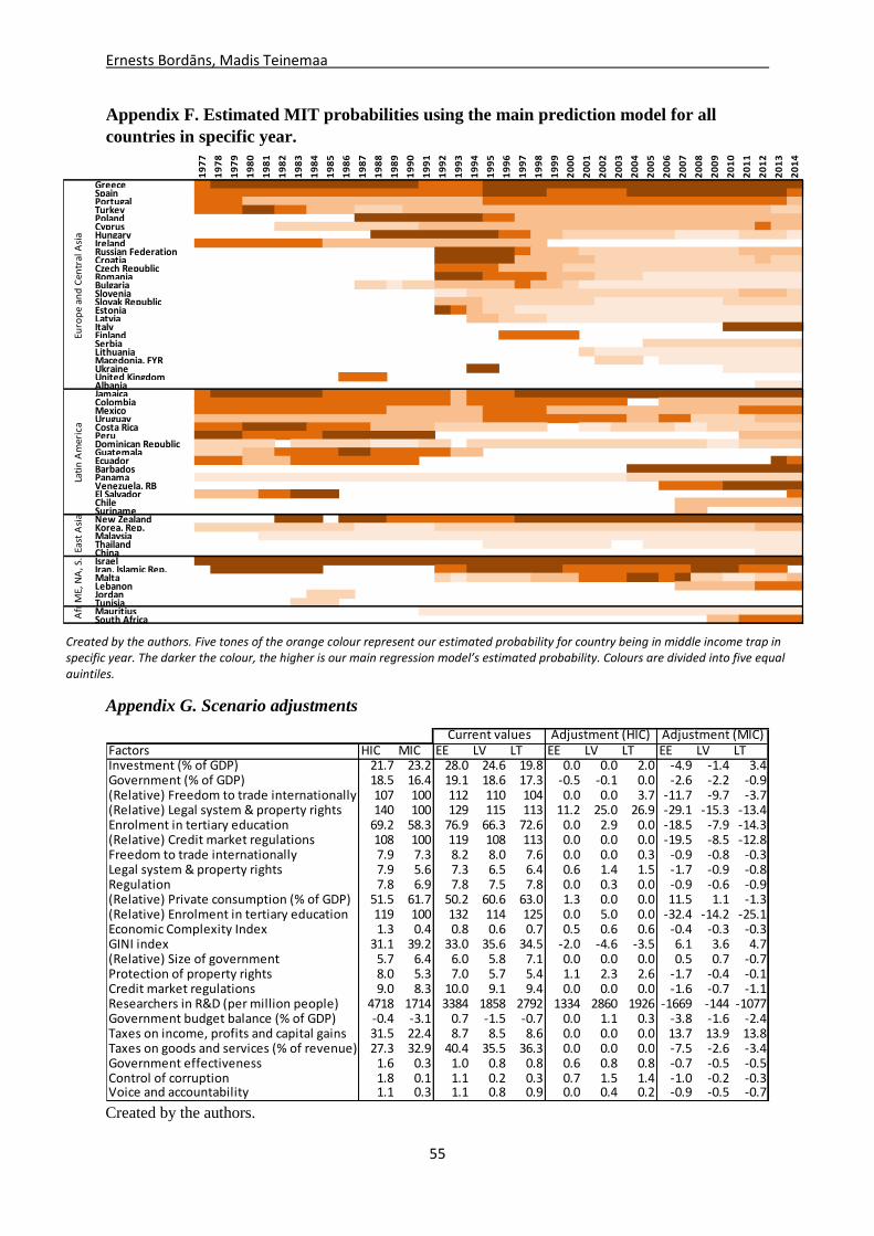
Ernests Bordāns, Madis Teinemaa
55
Appendix F. Estimated MIT probabilities using the main prediction model for all
countries in specific year.
Appendix G. Scenario adjustments
Factors HIC MIC EE LV LT EE LV LT EE LV LTInvestment (% of GDP) 21.7 23.2 28.0 24.6 19.8 0.0 0.0 2.0 -4.9 -1.4 3.4Government (% of GDP) 18.5 16.4 19.1 18.6 17.3 -0.5 -0.1 0.0 -2.6 -2.2 -0.9(Relative) Freedom to trade internationally 107 100 112 110 104 0.0 0.0 3.7 -11.7 -9.7 -3.7(Relative) Legal system & property rights 140 100 129 115 113 11.2 25.0 26.9 -29.1 -15.3 -13.4Enrolment in tertiary education 69.2 58.3 76.9 66.3 72.6 0.0 2.9 0.0 -18.5 -7.9 -14.3(Relative) Credit market regulations 108 100 119 108 113 0.0 0.0 0.0 -19.5 -8.5 -12.8Freedom to trade internationally 7.9 7.3 8.2 8.0 7.6 0.0 0.0 0.3 -0.9 -0.8 -0.3Legal system & property rights 7.9 5.6 7.3 6.5 6.4 0.6 1.4 1.5 -1.7 -0.9 -0.8Regulation 7.8 6.9 7.8 7.5 7.8 0.0 0.3 0.0 -0.9 -0.6 -0.9(Relative) Private consumption (% of GDP) 51.5 61.7 50.2 60.6 63.0 1.3 0.0 0.0 11.5 1.1 -1.3(Relative) Enrolment in tertiary education 119 100 132 114 125 0.0 5.0 0.0 -32.4 -14.2 -25.1Economic Complexity Index 1.3 0.4 0.8 0.6 0.7 0.5 0.6 0.6 -0.4 -0.3 -0.3GINI index 31.1 39.2 33.0 35.6 34.5 -2.0 -4.6 -3.5 6.1 3.6 4.7(Relative) Size of government 5.7 6.4 6.0 5.8 7.1 0.0 0.0 0.0 0.5 0.7 -0.7Protection of property rights 8.0 5.3 7.0 5.7 5.4 1.1 2.3 2.6 -1.7 -0.4 -0.1Credit market regulations 9.0 8.3 10.0 9.1 9.4 0.0 0.0 0.0 -1.6 -0.7 -1.1Researchers in R&D (per million people) 4718 1714 3384 1858 2792 1334 2860 1926 -1669 -144 -1077Government budget balance (% of GDP) -0.4 -3.1 0.7 -1.5 -0.7 0.0 1.1 0.3 -3.8 -1.6 -2.4Taxes on income, profits and capital gains 31.5 22.4 8.7 8.5 8.6 0.0 0.0 0.0 13.7 13.9 13.8Taxes on goods and services (% of revenue) 27.3 32.9 40.4 35.5 36.3 0.0 0.0 0.0 -7.5 -2.6 -3.4Government effectiveness 1.6 0.3 1.0 0.8 0.8 0.6 0.8 0.8 -0.7 -0.5 -0.5Control of corruption 1.8 0.1 1.1 0.2 0.3 0.7 1.5 1.4 -1.0 -0.2 -0.3Voice and accountability 1.1 0.3 1.1 0.8 0.9 0.0 0.4 0.2 -0.9 -0.5 -0.7
Current values Adjustment (HIC) Adjustment (MIC)
19
77
19
78
19
79
19
80
19
81
19
82
19
83
19
84
19
85
19
86
19
87
19
88
19
89
19
90
19
91
19
92
19
93
19
94
19
95
19
96
19
97
19
98
19
99
20
00
20
01
20
02
20
03
20
04
20
05
20
06
20
07
20
08
20
09
20
10
20
11
20
12
20
13
20
14
GreeceSpainPortugalTurkeyPolandCyprusHungaryIrelandRussian FederationCroatiaCzech RepublicRomaniaBulgariaSloveniaSlovak RepublicEstoniaLatviaItalyFinlandSerbiaLithuaniaMacedonia, FYRUkraineUnited KingdomAlbaniaJamaicaColombiaMexicoUruguayCosta RicaPeruDominican RepublicGuatemalaEcuadorBarbadosPanamaVenezuela, RBEl SalvadorChileSurinameNew ZealandKorea, Rep.MalaysiaThailandChinaIsraelIran, Islamic Rep.MaltaLebanonJordanTunisiaMauritiusSouth AfricaA
fric
aM
E, N
A, S
. Asi
aEa
st A
sia
and
Pac
ific
Lati
n A
mer
ica
Euro
pe
and
Cen
tral
Asi
a
Created by the authors. Five tones of the orange colour represent our estimated probability for country being in middle income trap in specific year. The darker the colour, the higher is our main regression model’s estimated probability. Colours are divided into five equal quintiles.
Created by the authors.

Ernests Bordāns, Madis Teinemaa
56
Appendix H. MIT predictions for Baltics with “HIC” and “MIC” scenario adjustments
Appendix I. Predicted MIT probabilities for all countries in 2014.
Country MIT probability Country MIT probability Albania 0.35% Macedonia, FYR 0.65% Barbados 93.50% Malaysia 0.03% Bulgaria 1.12% Malta 27.50% Chile 14.86% Mauritius 0.78% China 0.46% Mexico 30.19% Colombia 16.49% New Zealand 96.03% Costa Rica 5.56% Panama 2.47% Croatia 8.67% Peru 16.85% Cyprus 23.82% Poland 16.26% Czech Republic 3.85% Portugal 23.20% Dominican Republic 4.58% Romania 0.45% Ecuador 68.28% Russian Federation 13.69% El Salvador 67.24% Serbia 5.89% Estonia 0.46% Slovak Republic 4.77% Greece 79.06% Slovenia 9.23% Hungary 1.96% South Africa 41.08% Israel 90.12% Spain 65.95% Italy 89.30% Thailand 0.13% Jamaica 94.27% Turkey 6.86% Korea, Rep. 13.79% Ukraine 1.59% Latvia 2.06% Uruguay 16.20% Lebanon 46.66% Venezuela, RB 85.89% Lithuania 1.82%
Scenario Model 1 Model 2 Model 3 Model 4 Model 5 Model 6 Model 7 Model 8 Model 9 Average
EE 0.50% 4.00% 0.90% 0.90% 2.80% 0.00% 1.20% 1.00% 0.70% 1.30%
EE - HIC 0.40% 3.10% 0.50% 0.50% 2.20% 0.00% 0.40% 0.30% 0.50% 0.90%
EE->HIC -0.10% -0.90% -0.50% -0.40% -0.60% 0.00% -0.80% -0.70% -0.30% -0.50%
EE - MIC 2.70% 11.00% 1.00% 4.00% 3.50% 12.30% 12.50% 7.50% 6.60% 6.80%
EE->MIC 2.20% 7.00% 0.10% 3.20% 0.70% 12.30% 11.20% 6.50% 5.90% 5.50%
LV 2.10% 6.00% 4.50% 4.40% 8.30% 0.10% 2.60% 13.10% 8.40% 5.50%
LV - HIC 1.20% 3.70% 1.70% 1.70% 6.00% 0.00% 0.70% 1.60% 2.90% 2.20%
LV->HIC -0.90% -2.40% -2.80% -2.70% -2.30% -0.10% -1.90% -11.50% -5.50% -3.30%
LV - MIC 4.00% 8.60% 5.40% 8.40% 8.20% 0.40% 11.60% 24.60% 25.70% 10.80%
LV->MIC 1.90% 2.60% 0.90% 4.10% -0.10% 0.30% 9.00% 11.50% 17.30% 5.30%
LT 1.80% 4.70% 1.70% 2.50% 4.20% 0.00% 2.20% 1.80% 0.80% 2.20%
LT - HIC 1.00% 2.80% 0.70% 0.90% 2.60% 0.00% 0.50% 0.30% 0.40% 1.00%
LT->HIC -0.90% -1.90% -1.00% -1.60% -1.60% 0.00% -1.70% -1.50% -0.40% -1.20%
LT - MIC 3.40% 7.80% 3.10% 4.80% 4.00% 0.10% 10.40% 7.40% 6.30% 5.20%
LT->MIC 1.60% 3.10% 1.40% 2.30% -0.20% 0.10% 8.30% 5.60% 5.50% 3.10%
Mean of trapped obs. 58.70% 43.60% 51.30% 54.60% 42.10% 54.10% 37.30% 41.70% 39.60% 47.00%
Mean of all obs. 31.60% 28.90% 29.50% 30.20% 26.50% 20.80% 22.20% 20.30% 19.50% 25.50%
Mean of non-trapped obs. 20.00% 22.80% 20.30% 20.10% 20.00% 10.60% 16.90% 13.80% 13.70% 17.60%
Difference 38.60% 20.90% 31.00% 34.50% 22.10% 43.50% 20.40% 27.90% 26.00% 29.40%
Created by the authors.
Created by the authors.

Ernests Bordāns, Madis Teinemaa
57
Appendix J. Data sources.
Created by the authors.
Descriptions Sources Start End # of obs. Descriptions Sources Start End # of obs.
Extensive trade diversification IMF 1962 2010 2149 Cooperation in labor-employer relations WEF 2006 2014 419
Enrolment in tertiary education WDI 1970 2014 1760 Diversion of public funds WEF 2006 2014 419
Domestic credit by financial sector (% of GDP) WDI 1997 2014 420 Wastefulness of government spending WEF 2006 2014 419
Pay and productivity WEF 2006 2014 419 Burden of government regulation WEF 2006 2014 419
Education expenditure (% of GDP) WDI 1970 2014 1575 Voice and accountability WGI 1996 2014 973
Government exp. on education (% of GDP) WDI 1970 2014 1575 Government efficiency WEF 2006 2014 419
Compensation of employees (% of expense) WDI 1990 2013 871 Control of corruption WGI 1996 2014 973
GDP per capita WDI 1955 2014 2154 Legal system & property rights EF 1970 2013 1627
Prevalence of foreign ownership WEF 2006 2014 419 Government effectiveness WGI 1996 2014 973
Availability of financial services WEF 2006 2014 270 Resource efficiency BTI 2004 2014 389
Domestic credit to private sector WDI 1997 2014 420 Protection of property rights EF 1995 2013 826
Credit market regulations EF 1970 2013 1751 Market Economy Status Index BTI 2004 2014 389
Technological adoption WEF 2006 2014 270 Ethical behavior of firms WEF 2006 2014 419
PCT patents, applications/million pop WEF 2006 2014 184 Corporate ethics WEF 2006 2014 419
Innovation and business sophistication WEF 2006 2014 380 Institutions WEF 2006 2014 419
Economic Freedom Index EF 1970 2013 1661 Ethics and corruption WEF 2006 2014 419
Self-employed (% of total employed) WDI 1980 2014 1165 Efficiency of legal framework in settling disp. WEF 2006 2014 308
Health expenditure (% of GDP) WDI 1995 2013 1004 Effect of taxation on incentives to invest WEF 2006 2014 142
Export diversification IMF 1962 2010 2149 Anti-corruption policy BTI 2004 2014 389
Global Competitiveness Index WEF 2006 2014 380 Rule of law (WGI) WGI 1996 2014 973
Total Factor Productivity PWT 1955 2011 1912 Efficienct use of talent WEF 2006 2014 419
Economic Complexity Index OEC 1964 2013 1912 GINI index WDI 1981 2013 1022
Researchers in R&D (per million people) WDI 1996 2014 744 Judicial independence (WEF) WEF 2006 2014 419
Labor force with tertiary education (% of total) WDI 1982 2014 901 Black market exchange rates EF 1970 2013 1776
Quality of overall infrastructure WEF 2006 2014 419 Policy coordination BTI 2004 2014 389
Urban population (% of total) WDI 1960 2014 2154 Political and social integration BTI 2004 2014 389
Population growth PWT* 1954 2014 2097 Sustainability BTI 2004 2014 389
Market capitalization to GDP WDI 1975 2014 1020 Welfare regime BTI 2004 2014 389
Government (% of GDP) PWT 1960 2014 2031 Civil rights BTI 2004 2014 389
Investment (% of GDP) PWT 1960 2014 1987 Accountability WEF 2006 2014 419
Agriculture (% of GDP) WDI 1960 2014 1537 No. of days to start a business WEF 2006 2014 401
Trade openness PWT 1955 2009 2147 Organization of the market and competition BTI 2004 2014 389
Regulatory trade barriers EF 1995 2013 830 Public institutions WEF 2006 2014 419
Tariffs EF 1970 2013 1712 Flexibility of wage determination WEF 2006 2014 419
Imports (% of GDP) WDI 1960 2014 2033 BTI Status Index (democracy and market) BTI 2004 2014 389
Freedom to trade internationally EF 1970 2013 1714 Rule of law (BTI) BTI 2004 2014 389
Mean tariff rate (% ) WDI 1988 2013 1116 Social capital BTI 2004 2014 389
Exports (% of GDP) WDI 1960 2014 2033 Regulation EF 1970 2013 1614
Price level of imports PWT 1955 2011 2097 Country capacity to retain talent WEF 2006 2014 142
Current account balance WDI 1980 2015 1531 Irregular payments and bribes WEF 2006 2014 270
Price level of exports PWT 1955 2011 2097 Taxes on goods and services (% of revenue) WDI 1990 2013 855
Inflation WDI 1961 2014 1851 Stateness (BTI) BTI 2004 2014 389
Government budget balance (% of GDP) WDI 1990 2013 857 Regulatory Quality WGI 1996 2014 973
Price level of capital stock PWT 1955 2011 2097 Country capacity to attract talent WEF 2006 2014 142
FDI, net inflows (% of GDP) WDI 1970 2014 1738 Judicial independence (EF) EF 1995 2013 821
Macroeconomic environment WEF 2006 2014 419 Taxes on income, profits and capital gains WDI 1990 2013 862
Standard deviation of inflation EF 1970 2013 1761 Steering capability BTI 2004 2014 389
Access to Sound Mony EF 1970 2013 1772 Undue influence WEF 2006 2014 419
Interest rate spread (% ) WDI 1960 2014 1367 Top marginal tax rate EF 1970 2013 1516
Money growth EF 1970 2013 1717 Labor market regulations EF 1970 2013 1070
Employment of population (% ) PWT* 1955 2014 2077 Impartial courts EF 1995 2013 933
Region GDP growth WDI* 1960 2014 2154 Ease of access to loans WEF 2006 2014 419
Real effective exchange rate Bruegel 1960 2015 2097 Resolving insolvency EODB 2003 2015 479
Income level relative to trading partners WDI & 1960 2014 2147
*Compiled by authors using data from given source.
Eco
no
mic
Dev
elo
pm
en
tM
acro
eco
no
mic
En
vir
on
men
t
Go
vern
an
ce
Data gathered from the World Bank, World Development Indicators (WDI), Penn World Tables (PWT), Economic Freedom of the World by the Fraser Institute (EF), Global Competitiveness Report by
World Economic Forum (WEF), Bertelsmann Stiftung Index (BTI), Bruegel datasets, Ease of Doing Business (EODB) and World Governance Indices (WGI). As BTI surveys are conducted over two years
before reporting, we lag all data by two years to more appropriately correspond to the year of possible trap. Similarly, we lag all GCR variables by one year because of many variables that actually
correspond to previous years.