Balancing Budgets and Need during Recessions

Balancing Budgets and Need during Recessions California’s Safety Net Programs

Technical Appendices

CONTENTS

Appendix A. Past Budget Decisions Affecting Health and Social Safety Net Programs

Appendix B. Poverty Quantitative Analyses

Appendix C. Caseload Analyses: CalWORKs and SSI/SSP

Patrick Murphy, Caroline Danielson, Shannon McConville, Jennifer Paluch, and Tess Thorman

Supported with funding from the California Wellness Foundation

https://www.ppic.org/publication/balancing-budgets-and-need-during-recessions-californias-safety-net-programs/

https://www.ppic.org/publication/balancing-budgets-and-need-during-recessions-californias-safety-net-programs/

https://www.ppic.org/

PPIC.ORG Technical Appendices Balancing Budgets and Need during Recessions 2

Appendix A. Past Budget Decisions Affecting Health and Social Safety Net Programs

In order to understand the reach and the potential gaps in the social safety net during economic downturns we looked back at California enacted budget decisions over the past 20 years to see what budget and administrative levers the legislature used to balance the budget in good times and in bad. By organizing the budget decisions into revenue, spending and administrative levers, we aim to catalogue the legislature’s priorities and actions. The discussion below summarizes the approaches policymakers took, with a table presenting the timeline of decisions for Medi-Cal, CalWORKs, and SSI/SSP.

Medi-Cal Examining budget actions taken with regard to the three safety net programs specifically reveals more detail about the choices policymakers have made. In the case of Medi-Cal, for example, while a wide range of options may be available, past efforts have focused on:

Reducing the type of benefits offered. Federal regulations require states to provide a basic group of benefits to those eligible for coverage.1 Some states, California among them, have offered additional, optional services including dental, podiatry, and chiropractic coverage. In an effort to reduce spending, policymakers have cut some of these services during the past two recessions.

Reducing payments to providers. Medi-Cal participants do not pay for the services they receive. Instead, the program pays medical providers for services delivered to beneficiaries. The rates paid are set by the state. During recessions, policymakers have made cuts to these rates: not reducing the services covered, but how much is paid to the individuals and organizations that delivered the care.

Increasing federal support. In both of the last two recessions, the federal government has increased the federal medical assistance program (FMAP) percentage which determines the level of matching dollars provided to each state. In 2009, the FMAP rate rose from 50 percent to 61.59 percent adding $2.4 billion to revenue flowing into the state that year and the next.

There were numerous other changes to the Medi-Cal program such as reducing the payments made to counties to administer the program and instituting co-pays for some patients. In terms of the impact of these cuts, policymakers favored options that refrained from reducing access2 to basic medical services for low-income residents. The reduction in the type of services provided likely affects the care provided for some individuals. Also, reducing the rates for providers may have an indirect impact on access. The rate reduction essentially shifted some of the costs of balancing the budget to those providers, who, in turn, may decide to stop offering services to Medi-Cal clients. Table A1 provides an annual summary of actions taken between 1999 and 2019.

1 https://www.medicaid.gov/medicaid/benefits/list-of-benefits/index.html 2 It is worth noting that in 2003, the state did increase the frequency in which beneficiaries had to verify their eligibility. Requiring verification more often – moving for example from every 12 months to every 6 months – results in individuals being moved off the rolls more quickly.



TABLE A1 Medi-Cal summary

Revenue-related levers

Spending-related levers

Administrative levers

Med

i-Cal

de

sign

ated

re

venu

e /a

Tax

on

prov

ider

s

FMAP

rate

/b

Parti

cipa

nt

co-p

aym

ents

Elig

ibilit

y fo

r be

nefit

s

Rep

ortin

g/

verif

icat

ion

Type

of

bene

fits/

co

vera

ge

Paym

ents

to

prov

ider

s

Cou

nty

adm

in

paym

ents

Incr

ease

d fra

ud

prev

entio

n

Dru

g pr

ocur

emen

t ch

ange

s

Del

ayin

g pa

ymen

ts to

pr

ovid

ers

Acco

untin

g ch

ange

s

1999 2000 + - 2001 + 2002 - - - 2003 - - - - 2004 + - - - 2005 - + - 2006 + + 2007 + + - 2008 + - - - 2009 - - - - 2010 - - - - 2011 + - - 2012 - - 2013 + + + + 2014 + - 2015 + + 2016 + + 2017 + + 2018 + + 2019

SOURCES: California Department of Finance historical budgets, LAO-California Spending Plans NOTES: + indicates an increase, - indicates a decrease. /a In 2001, from the tobacco settlement and in 2017 voters passed Proposition 56 raising the cigarette tax. /b in 2008 the FMAP rate was raised for two federal fiscal years. Recessionary periods are shaded.

CalWORKs During the past two recessions, a number of components of the CalWORKs program were changed during annual budget negotiations.

Reducing the size of grants paid. This can be accomplished a number of ways, such as forgoing a cost-of-living increase, capping the maximum payment, reducing or capping the size of a family for the purpose of calculating benefits. Of course, policymakers have also simply cut the size of the grants directly as well.

Changing eligibility and time limits. To reduce the number of people receiving assistance, the state has adjusted the eligibility requirements including steps such as shifts around what can be included in the activities adults may participate in for the work requirement.3 There have also been reductions in the length of time adults can receive

3 In the 2012-13 budget, the legislature adjusted the rules for what could be considered under the activities for the work requirement for greater flexibility to address barriers to employment and they also enacted a 24-month time limit for families limited who may receive payment under the more flexible work requirement. The time limit for the less flexible federal work requirement was longer at 48 months, however the federal assessment of work places heavier emphasis on employment not a broader definition allowed by the state to include activities such as education, training, or mental health and substance abuse treatment.



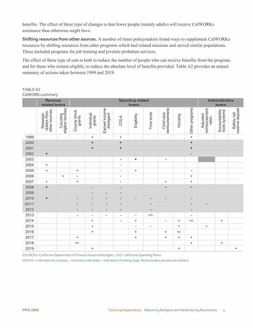
benefits. The effect of these type of changes is that fewer people (mainly adults) will receive CalWORKs assistance than otherwise might have.

Shifting resources from other sources. A number of times policymakers found ways to supplement CalWORKs resources by shifting resources from other programs which had related missions and served similar populations. These included programs for job training and juvenile probation services.

The effect of these type of cuts is both to reduce the number of people who can receive benefits from the program, and for those who remain eligible, to reduce the absolute level of benefits provided. Table A2 provides an annual summary of actions taken between 1999 and 2019.

TABLE A2 CalWORKs summary

Revenue related levers

Spending related levers

Administrative levers

Rea

ssig

n do

llars

from

ot

her s

ourc

es

Cou

ntin

g el

igib

le fa

milie

s

Cou

nty

bloc

k gr

ants

Indi

vidu

al

gran

ts

Earn

ed in

com

e di

sreg

ard

CO

LA

Elig

ibilit

y

Tim

e lim

its

Chi

ld c

are

reim

burs

emen

ts

Hou

sing

Oth

er p

rogr

ams

Adju

sted

re

imbu

rsem

ent

rate

s

Acco

unta

bilit

y to

ols

syst

ems

Safe

ty n

et

rese

rve

depo

sit

1999 + + + 2000 + + + 2001 + + + 2002 + - 2003 - + - 2004 + - 2005 + + - + - 2006 + - - + 2007 + + - + + 2008 + - - ~ ~ 2009 - - - 2010 + - - - - - - - - 2011* - - - - - - - 2012 - - - - - - 2013 - - - - - +/- - 2014 + - + - + +/- + 2015 + - - + + 2016 + + + +/- 2017 + + + + + 2018 +/- + + 2019 + + +

SOURCES: California Department of Finance historical budgets, LAO- California Spending Plans

NOTES: + indicates an increase, - indicates a decrease ~ indicated a funding swap. Recessionary periods are shaded.



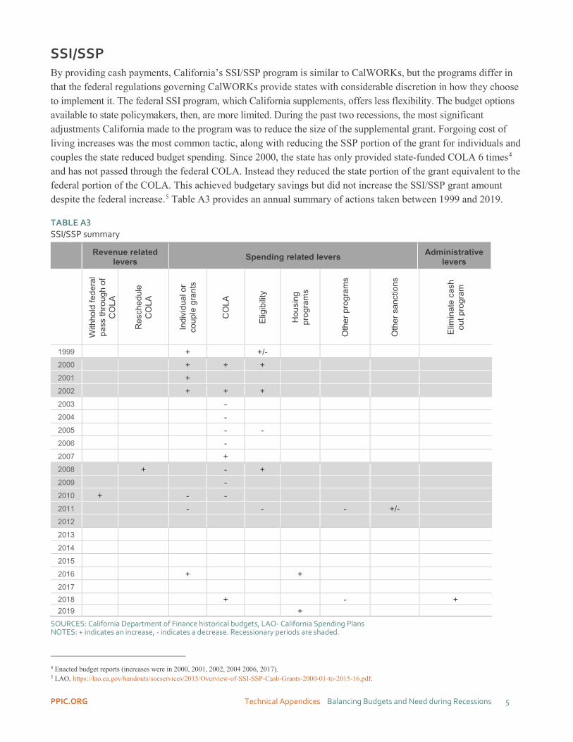
SSI/SSP By providing cash payments, California’s SSI/SSP program is similar to CalWORKs, but the programs differ in that the federal regulations governing CalWORKs provide states with considerable discretion in how they choose to implement it. The federal SSI program, which California supplements, offers less flexibility. The budget options available to state policymakers, then, are more limited. During the past two recessions, the most significant adjustments California made to the program was to reduce the size of the supplemental grant. Forgoing cost of living increases was the most common tactic, along with reducing the SSP portion of the grant for individuals and couples the state reduced budget spending. Since 2000, the state has only provided state-funded COLA 6 times4 and has not passed through the federal COLA. Instead they reduced the state portion of the grant equivalent to the federal portion of the COLA. This achieved budgetary savings but did not increase the SSI/SSP grant amount despite the federal increase.5 Table A3 provides an annual summary of actions taken between 1999 and 2019.

TABLE A3 SSI/SSP summary

SOURCES: California Department of Finance historical budgets, LAO- California Spending Plans NOTES: + indicates an increase, - indicates a decrease. Recessionary periods are shaded.

4 Enacted budget reports (increases were in 2000, 2001, 2002, 2004 2006, 2017). 5 LAO, https://lao.ca.gov/handouts/socservices/2015/Overview-of-SSI-SSP-Cash-Grants-2000-01-to-2015-16.pdf.

Revenue related levers Spending related levers Administrative

levers

With

hold

fede

ral

pass

thro

ugh

of

CO

LA

Res

ched

ule

CO

LA

Indi

vidu

al o

r co

uple

gra

nts

CO

LA

Elig

ibilit

y

Hou

sing

pr

ogra

ms

Oth

er p

rogr

ams

Oth

er s

anct

ions

Elim

inat

e ca

sh

out p

rogr

am

1999 + +/- 2000 + + + 2001 + 2002 + + + 2003 - 2004 - 2005 - - 2006 - 2007 + 2008 + - + 2009 - 2010 + - - 2011 - - - +/- 2012 2013 2014 2015 2016 + + 2017 2018 + - + 2019 +


https://lao.ca.gov/handouts/socservices/2015/Overview-of-SSI-SSP-Cash-Grants-2000-01-to-2015-16.pdf


Other measures In addition to making changes to the parameters of the three programs, policymakers also resorted to one-time measures or fund shifts as a way to address a budget problem in a given year. These efforts to find savings are not limited to recession level budget crises. Some of the changes produced modest savings, such as counting spending by the State Department of Education on child care for families who are eligible for CalWORKs (rather than the number receiving CalWORKs), scored at $86 million in 2005.6 Others represented more significant dollar amounts, such as the 2003 change that shifted Medi-Cal from an accrual to a cash basis accounting for the program.7 The LAO recently estimated that undoing that change would cost $2.6 billion now.8

Appendix B. Poverty Quantitative Analyses

In our main analysis of poverty trends, we use American Community Survey (ACS) data aggregated at the county- or county/group- level to model the relationship between unemployment rates and the share of nonelderly Californians that fall below certain poverty thresholds that roughly equate to program eligibility requirements. The approach is in the spirit of Moffitt (1999). Although each safety net program has different income eligibility levels and rules regarding how income is counted, we use ratios of the federal poverty level as proxies for eligibility. We use the deep poverty threshold – under 50 percent of the federal poverty level (FPL) -- as a proxy for CalWORKs eligibility; 100 percent FPL as a proxy for SSI/SSP eligibility for adults; 150 percent for Medi-Cal eligibility for adults, and 200 percent FPL as a proxy for children’s eligibility for SSI/SSP and Medi-Cal.

We estimate county panel fixed effects models where dependent variables are the share of residents in the demographic group in the county/county group that fall below the different poverty thresholds. These are estimated from the ACS. The key independent variable is the local labor market unemployment rate, from the Bureau of Labor Statistics. We use labor market unemployment rates rather than county unemployment rates in recognition that in several regions of the state the local labor market is larger than just a single county. All models include county/county group and year fixed effects to control for time invariant characteristics across areas, and exclude counties/county groups with ACS sample sizes under 20. We also omit models for people reporting another race/ethnicity due to small sample sizes. Estimates are identified by variation in the timing and severity of the Great Recession (as measured by local unemployment rates) across counties in California.

Table B1 shows results from regression models for poverty among all Californians age 0-64 as well as for different population groups including children, non-elderly adults with children, and non-elderly adults without children. Table B2 presents the same models, but adds two annual lags of the local unemployment rate, an approach commonly taken in the literature examining effects of the economy on poverty and on means-tested program participation.

In the case of Table B1, we find positive and significant associations. For example, for every one percentage point increase in the unemployment rate, the deep poverty rate (<50% FPL) rises between 0.33 and 0.84 percentage points. Effects are generally within the confidence interval of the estimates across the columns of the table. 6 This measure, coming just after the dom-com recession saved $86 million in 2005. 7 An accrual approach to Medi-CAL would account for a payment on the date the obligation is incurred – e.g., when a doctor bills the program for a service provided. A cash basis would not count that expense until the payment is actually made, which would likely be several weeks later. By making the shift, the state would push a share of program’s expenses out of one fiscal year and into another, lowering the cost of the program for that year. Of course, it represents a paper savings, as the payments still are made. Very few states use a cash basis for accounting for their Medicaid programs. 8 https://lao.ca.gov/Publications/Report/3988


https://lao.ca.gov/Publications/Report/3988


When models include lags, estimated associations are larger by at least 25 percent (shown in the “sum of coefficients” rows in Table B2). In Figure 5 in the report, we use the smaller estimated effects of the economy (from Table B1) to construct the number of adults and children in poverty under mild and moderate recession scenarios.

We estimate the population falling under 100% of FPL in a mild or a moderate recession by multiplying the coefficients in the second column of Table B1 by the percentage point increase in the unemployment rate during a recent, mild recession (the dot-com bust in 2000, when the statewide unemployment rate increased by 1.9 points) and a recent, moderate recession (the early 1990s recession, when the statewide unemployment rate increased by 4.0 points). We then multiply these coefficients by the estimated number of people in each of the three population groups (children under 19, adults 19-64 living in households with any children, and adults 19-64 living in households with no children) according to the California sample of the 2017 ACS. Finally, we round the results to the nearest 10,000.

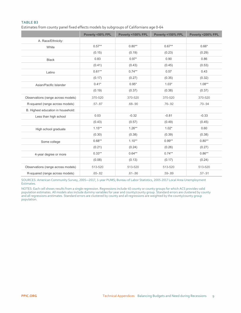
To assess whether recessions affect poverty levels differently by demographic groups and by education groups, we also estimated separate regressions within these groups. Table B3 shows these results. The models are analogous to those shown in Table B1, although due to sample size constraints we do not present estimates separately for children versus adults. While the coefficients on the contemporaneous unemployment rate from these models are typically positive and significant, the differences across race/ethnic groups and across levels of highest education are typically not statistically different from the base category. There is scattered significance comparing coefficients from models for those with a college degree or more to models estimated for those with lower educational attainment. At the same time, estimates imply substantive differences across the groups shown—even though they are not estimated precisely enough to show statistically significantly differences.

TABLE B1 Estimates from county panel fixed effects models by age group and family composition

Poverty <50% FPL Poverty <100% FPL Poverty <150% FPL Poverty <200% FPL

A. Children (age 0-18)

Contemporaneous unemployment rate 0.84** 1.14** 0.94** 0.69* (0.16) (0.29) (0.32) (0.33)

B. Adults (age 19-64) with children

Contemporaneous unemployment rate 0.65** 0.95** 0.76* 0.66*

(0.15) (0.25) (0.29) (0.31)

C. Adults (age 19-64) without children

Contemporaneous unemployment rate 0.33* 0.60** 0.80** 0.91** -0.16 -0.16 -0.19 -0.23

Observations (range across models) 520 520 520 520

R-squared (range across models) .87-.89 .91-.92 .92-.94 .92-.96

SOURCES: American Community Survey, 2005—2017, 1-year PUMS; Bureau of Labor Statistics, 2005-2017 Local Area Unemployment Estimates.

NOTES: Each cell shows results from a single regression. All models also include dummy variables for year and county/county group. Regressions include 40 county or county groups for which ACS provides valid population estimates. Standard errors are clustered by county and all regressions are weighted by the county/county group population.



TABLE B2 Estimates from county panel fixed effects models by age group and family composition with lagged effects of the economy


A. Children (age 0-18)

Contemporaneous unemployment rate 0.12 0.29 0.04 -0.28

(0.29) (0.31) (0.29) (0.27)

Unemployment rate lagged 1 year 0.52 0.55 0.62 0.49

(0.42) (0.57) (0.51) (0.42)

Unemployment rate lagged 2 years 0.41 0.60 0.57 0.86*

(0.27) (0.45) (0.35) (0.33)

Sum of coefficients 1.05** 1.44** 1.23** 1.07*

B. Adults (age 19-64) with children

Contemporaneous unemployment rate 0.16 0.13 -0.29 -0.49

(0.20) (0.24) (0.33) (0.31)

Unemployment rate lagged 1 year 0.29 0.54 0.82 0.71

(0.26) (0.39) (0.50) (0.45)

Unemployment rate lagged 2 years 0.37 0.56 0.55 0.83*

(0.20) (0.35) (0.34) (0.39)

Sum of coefficients 0.82** 1.23** 1.08** 1.05*

C. Adults (age 19-64) without children

Contemporaneous unemployment rate -0.07 0.14 0.20 0.35

(0.16) (0.19) (0.21) (0.21)

Unemployment rate lagged 1 year -0.22 -0.25 -0.05 -0.29

(0.26) (0.31) (0.42) (0.42)

Unemployment rate lagged 2 years 0.91** 1.05** 0.98** 1.25**

(0.23) (0.26) (0.28) (0.33)

Sum of coefficients 0.62** 0.94** 1.13** 1.31**

Observations (range across models) 520 520 520 520



NOTES: Each cell shows results from a single regression. All models also include dummy variables for year and county/county group. Regressions include 40 county or county groups for which ACS provides valid population estimates. Standard errors are clustered by county and all regressions are weighted by the county/county group population.



TABLE B3 Estimates from county panel fixed effects models by subgroups of Californians age 0-64


A. Race/Ethnicity:

White 0.57** 0.80** 0.67** 0.66*

(0.15) (0.19) (0.23) (0.29)

Black 0.83 0.97* 0.90 0.86

(0.41) (0.43) (0.45) (0.53)

Latino 0.61** 0.74** 0.57 0.43

(0.17) (0.27) (0.35) (0.32)

Asian/Pacific Islander 0.41* 0.95* 1.03* 1.08**

(0.19) (0.37) (0.38) (0.37)

Observations (range across models) 370-520 370-520 370-520 370-520


B. Highest education in household:

Less than high school 0.03 -0.32 -0.81 -0.33

(0.43) (0.57) (0.49) (0.45)

High school graduate 1.15** 1.26** 1.02* 0.60

(0.30) (0.38) (0.39) (0.38)

Some college 0.68** 1.10** 0.99** 0.80**

(0.21) (0.24) (0.26) (0.27)

4-year degree or more 0.33** 0.64** 0.74** 0.86**

(0.08) (0.13) (0.17) (0.24)

Observations (range across models) 513-520 513-520 513-520 513-520



NOTES: Each cell shows results from a single regression. Regressions include 40 county or county groups for which ACS provides valid population estimates. All models also include dummy variables for year and county/county group. Standard errors are clustered by county and all regressions arstimates. Standard errors are clustered by county and all regressions are weighted by the county/county group population.



Appendix C. Caseload Analyses: CalWORKs and SSI/SSP

CalWORKs caseloads Figure C1 provides clear descriptive evidence that the program is countercyclical. In the figure, 2007/08 per capita caseloads is the baseline, allowing a direct comparison of the size of the caseload over the period 2002 to 2018. Compared with 2007/08, the share of adults on CalWORKs grew by 41 percent and the share of children with CalWORKs assistance by 26 percent by January 2011.

FIGURE C1 CalWORKs has been a countercyclical program in California

SOURCE: Author calculations from CDSS CA237CW reports for 2002/03-2018/19 and Census 5-year population estimates.

NOTE: Per capita number of child and adult recipients as compared to baseline year shown. Baseline is average per capita recipients in state fiscal year 2007-08.

Table C1 shows regressions of the natural log of annual average per capita county CalWORKs recipients from 2005-2017. Numerators are from CDSS CA237 reports while denominators are from Census population estimates. The first of each pair of models includes the log of the official (<50%) deep child poverty rate while the second includes the log of the child poverty rate. Poverty rates are calculated from the 1-year ACS public-use microdata. Forty-one counties and groups of California counties are identified in the ACS. All models include year dummies and dummies for county of residence.

According to these models, the elasticity of the caseload with respect to child poverty is 0.13-0.14, while there is no significant relationship between deep child poverty and caseloads. Given that the ACS does not support an accurate determination of CalWORKs eligibility, it is not surprising that the point estimates we obtain are below 1. Nonetheless, because the point estimates are so far below 1, these descriptive regressions suggest that poverty increases outstripped caseload increases in California. This could be the case both because access to CalWORKs is not universal among poor families, even in good economic times, or because cuts reduced access to CalWORKs during and after the last recession, or both.

-50

-40

-30

-20

-10

0

10

20

30

40

50

% c

hang

e re

lativ

e to

200

7

Children

Adults



TABLE C1. Regression-adjusted relationship between poverty and CalWORKs caseloads

(1) (2) (3) (4) (5) (6)

Log (total recipients) Log (child recipients) Log (adult recipients) Log (child deep poverty rate) 0.030 0.032 0.020

(0.019) (0.020) (0.020) Log (child poverty rate) 0.14** 0.13** 0.14**

(0.040) (0.041) (0.047)

Observations 520 520 520 520 520 520 R-squared 0.980 0.982 0.976 0.977 0.972 0.973

Standard errors in parentheses

** p<0.01, * p<0.05

Tables C2 and C3 provide evidence of the regression-adjusted relationship between CalWORKs caseloads—as measured by entries, exits, and caseloads—and the economy (as measured by the unemployment rate). The dependent variables are the natural log of per capita county caseloads, where the numerator is drawn from CDSS CA237 reports and the denominator from Census population estimates. Unemployment rates are from the Bureau of Labor Statistics’ Local Area Unemployment Statistics (LAUS) program. We include lags of the unemployment rate in some models to capture the sluggish response of caseloads to changes in the economy. All models include dummy variables for month-year of the analysis and county fixed effects. The month-year dummies capture statewide changes in caseloads due to policy changes that changed eligibility for the program throughout this time period—implying that we are, to a first order, adjusting for the shortening of time limits, the reduction in benefits, and the changes to work requirements that occurred during and after the Great Recession.

The models show clear evidence of a positive relationship between applications for CalWORKs—and the total number of CalWORKs recipients—and the economy over the time period 2002-2018. Adjusting for changes to eligibility (using fixed effects for time), we find a similar percent increase in the caseload of child recipients (0.014) as adult recipients (0.013).

Columns 3 and 4 of Table C2 also provide mixed evidence of a drop in exits when the employment rate rises. The point estimate is negative and significant in the model that includes the current unemployment rate (-0.017), and is negative and larger (-0.028) in the model that includes 5 year lagged unemployment rates—but is less precisely estimated.



TABLE C2. Regression-adjusted relationship between the unemployment rate and CalWORKs applications (entries) and exits

(1) (2) (3) (4) Applications Exits

Unemployment rate 0.011* -0.0015 -0.017** -0.040** (0.0052) (0.0081) (0.0045) (0.013) Lagged 1 year: unemp. rate

0.00098 0.011

(0.0080) (0.0099) Lagged 2 years: unemp. rate

0.0045 -0.0022


0.0063 -0.0020


0.0010 0.015*


0.0059 0.0094

(0.0071) (0.0084) Summed coeff. 0.0037** -0.028 Observations 11,395 11,395 11,349 11,349 R-squared 0.870 0.871 0.824 0.826


** p<0.01, * p<0.05

NOTE: Missing observations reflect 0 applications or exits in small counties in a few months.

TABLE C3. Regression-adjusted relationship between the unemployment rate and CalWORKs caseloads

(1) (2) (3) (4) (5) (6) Recipients Child recipients Adult recipients

Unemployment rate 0.014** -0.0035 0.014** -0.0046 0.013* -0.0045 (0.0044) (0.0079) (0.0047) (0.0084) (0.0050) (0.0082) Lagged 1 year: unemp. rate -0.00015 0.00035 0.0019 (0.0049) (0.0050) (0.0068) Lagged 2 years: unemp. rate 0.0019 0.0032 -0.0025 (0.0068) (0.0064) (0.0062) Lagged 3 years: unemp. rate 0.0091* 0.0094* 0.011* (0.0043) (0.0042) (0.0054) Lagged 4 years: unemp. rate 0.011** 0.0095** 0.017** (0.0034) (0.0034) (0.0050) Lagged 5 years: unemp. rate 0.0043 0.0058 -0.0025 (0.0047) (0.0042) (0.0055) Summed coeff. 0.016** 0.015** 0.014** Observations 11,474 11,474 11,474 11,474 11,462 11,462 R-squared 0.938 0.940 0.926 0.929 0.933 0.934

Standard errors in parentheses ** p<0.01, * p<0.05



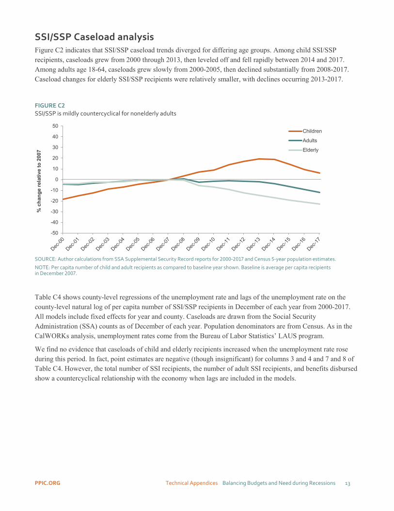
SSI/SSP Caseload analysis Figure C2 indicates that SSI/SSP caseload trends diverged for differing age groups. Among child SSI/SSP recipients, caseloads grew from 2000 through 2013, then leveled off and fell rapidly between 2014 and 2017. Among adults age 18-64, caseloads grew slowly from 2000-2005, then declined substantially from 2008-2017. Caseload changes for elderly SSI/SSP recipients were relatively smaller, with declines occurring 2013-2017.

FIGURE C2 SSI/SSP is mildly countercyclical for nonelderly adults

SOURCE: Author calculations from SSA Supplemental Security Record reports for 2000-2017 and Census 5-year population estimates.

NOTE: Per capita number of child and adult recipients as compared to baseline year shown. Baseline is average per capita recipients in December 2007.

Table C4 shows county-level regressions of the unemployment rate and lags of the unemployment rate on the county-level natural log of per capita number of SSI/SSP recipients in December of each year from 2000-2017. All models include fixed effects for year and county. Caseloads are drawn from the Social Security Administration (SSA) counts as of December of each year. Population denominators are from Census. As in the CalWORKs analysis, unemployment rates come from the Bureau of Labor Statistics’ LAUS program.

We find no evidence that caseloads of child and elderly recipients increased when the unemployment rate rose during this period. In fact, point estimates are negative (though insignificant) for columns 3 and 4 and 7 and 8 of Table C4. However, the total number of SSI recipients, the number of adult SSI recipients, and benefits disbursed show a countercyclical relationship with the economy when lags are included in the models.

-50

-40

-30

-20

-10

0

10

20

30

40

50

% c

hang

e re

lativ

e to

200

7

Children

Adults

Elderly



TABLE C4. SSI/SSP recipients and benefit amounts disbursed

(1) (2) (3) (4) (5) (6) (7) (8) (9) (10) Total Children 0-17 Adult 18-64 Elderly 65+ Total benefits

Unemployment rate

0.0014 -0.00020 -0.010 -0.012 0.0039 0.0037 -0.0051 -0.0050 0.0066 -0.0017

(0.0042) (0.0029) (0.0071) (0.0085) (0.0060) (0.0061) (0.0052) (0.0059) (0.0063) (0.0041) Lagged 1 year: unemp. rate

0.00094 -0.0021 0.0016 -5.2e-06 0.016*

(0.0026) (0.0069) (0.0041) (0.0036) (0.0069) Lagged 2 years: unemp. rate

0.0051* 0.0017 -0.00065 0.00054 -0.0034


0.00047 0.0073 0.0060 0.00041 0.0019


0.0018 -0.0050 0.000038 0.000038 0.0021


0.0079* -0.0034 0.0095* 0.0021 0.0097*

(0.0032) (0.0048) (0.0042) (0.0042) (0.0044) Summed coeff. 0.016** -0.013 0.020* -0.0018 0.024** Observations 1,044 1,044 1,006 1,006 1,037 1,037 1,011 1,011 1,044 1,044 R-squared 0.980 0.981 0.954 0.954 0.976 0.977 0.987 0.987 0.976 0.977


*** p<0.01, ** p<0.05, * p<0.10

NOTE: Missing observations reflect suppressed data for several small counties.


The Public Policy Institute of California is dedicated to informing and improving public policy in California through independent, objective, nonpartisan research.

Public Policy Institute of California 500 Washington Street, Suite 600 San Francisco, CA 94111 T: 415.291.4400 F: 415.291.4401 PPIC.ORG

PPIC Sacramento Center Senator Office Building 1121 L Street, Suite 801 Sacramento, CA 95814 T: 916.440.1120 F: 916.440.1121




Balancing Budgets and Need during Recessions

Documents

Transcript of Balancing Budgets and Need during Recessions