Balance-Sheet Diversification in General Equilibrium...

NBER WORKING PAPER SERIES

BALANCE-SHEET DIVERSIFICATION IN GENERAL EQUILIBRIUM: IDENTIFICATION AND NETWORK EFFECTS

Jonas HeipertzAmine Ouazad

Romain RancièreNatacha Valla

Working Paper 23572http://www.nber.org/papers/w23572

NATIONAL BUREAU OF ECONOMIC RESEARCH1050 Massachusetts Avenue

Cambridge, MA 02138July 2017

The views expressed herein are those of the authors and do not necessarily reflect the views of the National Bureau of Economic Research.

At least one co-author has disclosed a financial relationship of potential relevance for this research. Further information is available online at http://www.nber.org/papers/w23572.ack

NBER working papers are circulated for discussion and comment purposes. They have not been peer-reviewed or been subject to the review by the NBER Board of Directors that accompanies official NBER publications.

© 2017 by Jonas Heipertz, Amine Ouazad, Romain Rancière, and Natacha Valla. All rights reserved. Short sections of text, not to exceed two paragraphs, may be quoted without explicit permission provided that full credit, including © notice, is given to the source.

Balance-Sheet Diversification in General Equilibrium: Identification and Network EffectsJonas Heipertz, Amine Ouazad, Romain Rancière, and Natacha VallaNBER Working Paper No. 23572July 2017JEL No. G11,G15,G23

ABSTRACT

The paper uses disaggregated data on asset holdings and liabilities to estimate a general equilibrium model where each institution determines the diversification and size of the asset and liability sides of its balance-sheet. The model endogenously generates two types of financial networks: (i) a network of institutions when two institutions share common asset or liability holdings or when an institution holds an asset that is the liability of another. In both cases demand/supply decisions by one institution affect the value of other institutions' holdings/liabilities, (ii) a network of financial instruments implied by the distribution of assets and liabilities within and across institutions. A change in the price of one asset induces change in demand/supply for all other assets, thus generating price comovement. The general equilibrium analysis predicts the propagation of real, financial and regulatory shocks as well as the change in the network caused by the shock.

Jonas HeipertzParis School of [email protected]

Amine OuazadHEC Montreal3000, Chemin de la Cote Sainte CatherineH3T 2A7, Montreal, [email protected]

Romain RancièreDepartment of EconomicsUniversity of Southern CaliforniaLos Angeles, CA 90097and [email protected]

Natacha VallaEuropean Investment [email protected]

1 Introduction

The crisis of 2007-2008 has triggered considerable interest in the understanding of the role

of financial networks in the propagation of financial and real shocks, and in the emergence

of systemic risk in financial systems. When institutions share a common set of financial

assets and liabilities, price externalities make asset demand and supply decisions interde-

pendent across institutions. The resulting networks of institutions propagate shocks and

potentially generate financial fragility such as fire-sale spirals that weaken balance sheets.

Alternatively, the distribution of assets across and within institutions makes asset valua-

tion interdependent and the resulting network of financial instruments can trigger large

asset price comovement even between very different classes of assets. In contrast with net-

work propagation associated with bilateral exposure (i.e. counterparty risk) which could be

contained ex-post by targeted interventions, and prevented ex-ante by the development of

centrally-cleared markets, network propagation associated with price externalities is much

harder to contain.

While there is a large literature that characterizes the topology of such networks and

their associated fragility (Greenwood, Landier & Thesmar 2015, Acemoglu, Ozdaglar &

Tahbaz-Salehi 2015), their endogenous formation through market interaction and trade in

financial assets is still poorly understood.1

This paper puts forward and estimates a new framework which explains how both a

network of institutions and a network of financial instruments emerge out of a structural

general equilibrium model of trade in financial assets and liabilities among heterogeneous

institutions. The structural estimation of the model uses a dynamic factor structure for

the net demand of each asset of each institution (i.e. gross demand for the asset minus

liability of the same asset). This enables an identification of institutions’ key character-

istics: risk-aversion, cost of equity, and beliefs about future returns. The equilibrium net

asset positions jointly determine both a network of financial instruments and a network of

institutions. The structural estimation enables us to relate the shape of both networks and

the implied shock transmission to the characteristics and beliefs of the underlying institu-

tions. The structural approach also enables us to run counterfactual experiments. Such

experiments provide an understanding of the evolution of the financial networks’ structures

and of their shock transmission properties, in response to changes in capital requirements,

1By contrast, there is an established literature that looks at the endogenous formation of social networks(Jackson & Watts 2002, Goyal & Vega-Redondo 2005)

2

changes in the structure of shocks, and changes in institutions’ beliefs. This paper is to

the best of our knowledge the first to provide a direct structural link between net financial

asset trade in general equilibrium, network structure, and network effects.

In this version of the paper, the model is estimated on detailed flows of funds infor-

mation available for seven sectors of the French economy including a “rest of the world”

sector. In such estimation, an institution represents a sector. A subsequent version will

include a finer estimation based on detailed balance-sheets of individual institutions.2 The

sectoral balance-sheets provide information on 20 classes of assets and liabilities, including

traded securities, non-traded financial assets (e.g. loans), and real assets.

The estimation procedure follows two steps. In the first step, net asset demands by

institutional sector are estimated using a dynamic factor model. Both the factor struc-

ture and the loadings are allowed to vary across institutional sectors. The key finding is

that a small number of factors is able to explain the bulk of the variance in net demands.

Moreover, the factors exhibit a close correspondence with drivers of the Global cycle and

Eurozone cycle, as they respectively correlate with US and Euro policy rates, global GDP

growth and global trade growth, the VIX measure of implied global risk aversion, or inter-

est rates on government securities for the countries that were subject to the sovereign crisis

of 2011 (Greece, Ireland, Italy, Portugal and Spain). In the second step, the structural

parameters of the net asset demand model regarding institutions characteristics (risk aver-

sion and the cost of equity) and return beliefs, are obtained, through a mapping between

the factor structure of net demand and the factor structure of return beliefs. Finally, a

set of closed-form formulas enables then to fully characterize the network structure and to

obtain general equilibrium effects associated with a diffusion of a sector-specific shock in

the network.

A first set of results regards the analysis of return beliefs across institutions and across

assets. The model for return beliefs indeed explains up to 39 percent of the variance of

ex-post returns depending on the sector and instrument. Moreover, the cases when the

belief model fails to predict return are almost all related to the 2007-2008 crisis when some

institutional sectors made counter-cyclical net asset purchases, i.e. buying assets whose

returns are declining, for liquidity reasons (banking sector) or bailout purposes (public

sector).

A second set of results emerges from the analysis of the dual network of assets and

2The clearance for these confidential data has been obtained too late so that this estimation could beincluded on this graph.

3

institutions, and its implications for shock propagation. Network effects stemming from

the general equilibrium impact of a shock to the capital base of the banking sector on all

sectors including he banking sector itself reveal that: (i) such effects can be sizeable and,

in some sectors, of comparable – if not amplified - magnitude than those experienced by

the sector where the shock originated; (ii) they vary dramatically in size and scope across

sectors. This evidence vindicates the massive net asset demand shifts - out of banks into

the insurance sector - that could be observed in the aftermath of the 2007-2008 crisis as

a result of severe capital losses in the banking sector that preceded the euro sovereign

crisis.(Heipertz, Ranciere & Valla 2016).

This paper builds a bridge between two literatures, the literature on asset demand

among heterogeneous institutions (Koijen & Yogo 2016, Miranda-Agrippino & Rey 2015)

and that on financial networks structure and associated network effects (Eisenberg & Noe

2001, Elliott, Golub & Jackson 2014, Greenwood et al. 2015). The paper develops a

novel methodology that uses balance sheet information on asset and liability positions

of all sectors of the economy to estimate structurally a general equilibrium model of net

asset demand allowing for large sectoral heterogeneity in risk-aversion, beliefs, and cost of

equity. The estimated model generates endogenously a time-varying network of financial

instrument and a network of institutional sectors.

Another innovation of the paper is to use the full balance sheet of asset and liability for

all sectors of the French economy rather than focusing on asset allocation for just one sector,

such as the mutual fund sector. This approach turns out to be important as the 2007-2008

crisis generated considerable reshuffling in liability and asset positions across sectors. In

the case of France, the crisis of 2007-2008 led to a retrenchment of the banking sector

accompanied for an expansion of the insurance sector (Heipertz et al. 2016). While the use

of sector-level data allows to assess the general equilibrium effect of a sectoral shock on the

very same sector, it does not account for the role played by large net demand position of

individual institutions that net out at the sector level. Until the issue is addressed with the

use of individual institutional data, the network effects measured here could be considered

as conservative estimates of the importance of financial networks in the propagation of

shocks.

The paper contributes to the literature on the role of belief heterogeneity in asset

pricing (Berrada 2006, Gandhi & Serrano-Padial 2015) by using net asset demands to

estimate a model with a large dimension of heterogeneity (risk-aversion, beliefs, cost of

equity). The paper shares with Koijen & Yogo (2016) the objective of a structural model

4

that simultaneously matches asset demands and imposes market clearing but our approach

is very different. Rather than estimating a discrete choice model to understand the portfolio

choice of investors as a function of characteristics, we are using the factor structure of net

demands for assets to reveal the factor structure of the beliefs about asset returns and other

structural parameters. Price externalities are at the core of our network of institutions and

network of financial instruments as in Greenwood et al. (2015) but with the key difference

that the networks in our paper are derived from a general equilibrium model of net asset

trade rather than just assumed. In additon Greenwood et al. (2015) only deal common

asset holdings accross institutions when we also consider the role of assets and liabilities

holdings for the propagation of shocks. The factor structure of net demands emphasizes

the role of the global cycle as in Miranda-Agrippino & Rey (2015) but also stresses the

importance of Euro area specific factors in the dynamics of net demand.

2 Theoretical Framework

2.1 The Model

A finite number N of firms trade J financial instruments in each discrete time period

t = 1, 2, 3, . . . . In period t, each of the j = 1, 2, . . . , J financial instruments has a price pjt

and yields a stochastic return rjt at the end of the period.

Each firm i has a level of equity Eit in period t and seeks to maximize the expected

return on its equity by raising funds on the market (through the emission of liabilities) and

investing these raised funds and the firm’s equity in financial and real assets. Thus, each

firm i chooses a level of gross demand Dijt and gross supply Sijt for each of the J financial

instruments. Each additional unit of total demand for assets beyond the initial level equity

Eijt requires raising a corresponding additional unit of liability. Indeed, the firm’s balance

sheet satisfies the usual equality of assets and liabilities, formally:

D′it1J = S′it1J + Eit (1)

where Dit = (Di1t, . . . , Di2t)′ is the column vector of demands for each of the J instruments,

and Sit is the column vector of supplies. 1J is the column vector of ones of size J . Such

demand and supply choices, together with firm i’s initial equity level, make up both total

balance sheet size and its asset and liability diversification.

In order to maximize its return on equity, each firm i forms beliefs about the distribu-

5

tion of future returns rjt based on (i) a firm-specific and potentially sophisticated return

forecasting model, and (ii) on a firm-specific information set. Both model and information

are fundamentally unobservable to the econometrician. Such firm-specific forecasting exer-

cise yields a distribution of returns noted rijt. We will assume throughout that stochastic

beliefs about returns are not multicollinear and have strictly positive variances, which im-

plies that the variance-covariance of beliefs is symmetric, positive-definite. Noting rit the

firm-specific stochastic belief about returns, the firm’s net income is (Dit − Sit)′rit.

Each firm trades off the expected return and the expected variance of such stochastic

net income. The relative importance of variance for firm i is noted ρi.3 Alternatively,

firms can also maximize expected returns under a value-at-risk (VAR) constraint, where

the lagrange multiplier corresponding to such constraint is equivalently noted ρi. Formally

firm i demands and supplies assets in order to maximize

(Dit − Sit)′µit −

1

2ρi(Dit − Sit)

′Σit(Dit − Sit) (2)

where µit ≡ E [rit] ≡ E [rt|Ωit] is the J-vector of mean return beliefs and Σit ≡ V ar [rit] ≡V ar [rt|Ωit] is the J-square matrix of the variance-covariance of return beliefs. Both are

obtained by firm i given its information set and model, noted Ωit . The maximization

of (2) is performed under the funding constraint (1), as the total amount of outstanding

assets must equal the sum of initial equity and funds raised.

2.2 Net Demands and Cost of Equity

There exists a closed form solution for the balance sheet that maximizes the mean-variance

objective under the funding constraint as described in the following proposition.

Proposition 1. Each institution i’s net demand for assets depends on the first two mo-

ments of its return beliefs, its risk aversion, and its cost of capital. Formally, write

∆it = Dit − Sit the J-vector of net demands, then

∆it = Dit − Sit =1

ρiΣ−1it (µit − ηit1), (3)

3This mean-variance goal for a firm formally corresponds to the concept of absolute risk aversion in thecontext of household choice under uncertainty with Constant Absolute Risk Aversion (CARA).

6

where ηit is the scalar Lagrange multiplier of the funding constraint,

ηit =1′Σ−1

it µit − ρiEit1′Σ−1

it 1. (4)

The Lagrange multiplier ηit corresponding to constraint (1) is the cost of equity as the

marginal impact of an additional unit of equity in period t on the firm’s mean-variance

objective (2).

2.3 Market Equilibrium

The previous section has obtained the net demand of each financial instrument as a function

of (i) return beliefs, (ii) risk aversion and (iii) firm equity. While the beliefs about end-of-

period returns are institution-specific (each institution estimates a forecast of returns), the

asset price pjt is public information. In that sense, the uncertainty of a financial institution

is over future dividends and future asset values, not about the current price of the asset.

rijt =E[pjt+1 + djt+1|Ωit

]pjt

(5)

where pjt+1 is the price in period t + 1, djt+1 the dividend in period t + 1 and Ωit the

information set of institution i in period t. Thus net demand (3) is a function of asset

prices, and defines demand and supply curves for all instruments and all institutions.

To define an equilibrium, notice that the equity of firm i is a financial instrument

j(i) ∈ 1, 2, . . . , J supplied by firm i and demanded by (potentially) all other firms i′ 6= i,

so that equilibrium on the market for the equity j(i) of firm i is∑N

i′=1 ∆i′j(i)t = Eit. On

all other markets, the equilibrium condition is:∑N

i′=1 ∆i′jt = 0. Stack all Eit in a J-vector

Et whose j-th element is Eit if j(i) = j and 0 otherwise, then:

Definition 1. An equilibrium in period t is a J-vector of prices for each financial instru-

ment p∗t such that all J markets clear:

N∑i=1

∆it (p∗1t, p∗2t, . . . , p

∗Jt) = Et(p

∗1t, p

∗2t, . . . , p

∗Jt), (6)

where each ∆it (p∗t ) is a column vector of size J ; the institution-specific equilibrium vectors

of net demands are ∆∗it ≡∆it (p∗1t, p∗2t, . . . , p

∗Jt); and Et(p

∗t ) is a column vector of size J .

7

The equilibrium in such an economy exists, as shown in the following proposition:

Proposition 2. (Existence of an Equilibrium) There exists a price vector p∗t ∈ RJ

such that∑N

i=1 ∆it(p∗t ) = Et(p

∗t ).

An extension of the framework where the net demand vector includes Jexo exogenous

net demands (i.e. unaffected by prices), and Jendo endogenous net demands (i.e. defined

as in equation (3)), yields a similar result on the existence of equilibrium prices and net

demands.

2.4 Shock Propagation with Comparative Statics

The general equilibrium setting enables an analysis of propagation of a shock on funda-

mentals or beliefs. Indeed shocks cause shifts in individual firm net demands, which affect

market prices, and thus potentially all net demands in the economy. The general equilib-

rium analysis with comparative statics provides two dual networks, as shocks propagate

through (i) the network of financial instruments’ prices, and through (ii) the network of

institutions’ balance sheets.

2.4.1 Comparative Statics

Consider a shock dθ on one of the economy’s structural exogenous parameters θ . Possible

shocks dθ include shifts in the equity of a financial institution, shifts in the beliefs about

future returns, shifts in exogenous net demands, shifts in risk aversion, or the introduction

of a liquidity or capital constraint. The shock dθ can affect one or more institutions.

The total impact of a shock dθ on the net demand of each institution i = 1, 2, . . . , N

in year t is the sum of a partial equilibrium term, and a general equilibrium term. Indeed,

the total derivative of net demand w.r.t. the shock expands according to the chain rule

as:4d∆it

dθ=∂∆it

∂θ+

∂∆it

∂ log pt

d log ptdθ

, (7)

where ∂∆it∂θ is the partial equilibrium effect, and ∂∆it

∂ log ptthe sensitivity of net demand to the

prices of financial instruments. d log ptdθ is the market-wide shift in the vector of log prices,

4For the sake of clarity, we are considering a shock that does not affect equity directly, i.e. ∂Eit/∂θ = 0.If the shock has a direct impact on equity, the total derivative of net demand with respect to the shock isd∆itdθ

= ∂∆it∂θ

+ ∂∆it∂ log pt

d log ptdθ

+ ∂∆it∂Eit

∂Eit∂θ

. The following analysis can proceed in a similar fashion, adding

the term (∂∆it/∂Eit) · (∂Eit/∂θ) to the right-hand side of equation 7.

8

common to all institutions.

Starting from a market equilibrium (p∗, (∆∗it, i = 1, 2, . . . , I, t = 1, 2, . . . , T )), the shock

dθ affects net demands in a way that violates the equilibrium condition (6). The shift in

prices d log pt/dθ is the vector of price changes that restores equilibrium in each market.

Then the equality of shifts in demand and shifts in equity values,

N∑k=1

[∂∆kt

∂θ+

∂∆kt

∂ log pt

d log ptdθ

]=

∂Et

∂ log pt

d log ptdθ

, (8)

provides the general equilibrium price shift d log pt/dθ:

d log ptdθ

=

[∂Et

∂ log pt−

N∑k=1

∂∆kt

∂ log pt

]−1 [ N∑k=1

∂∆kt

∂θ

], (9)

In the short run, with a fixed number of shares in each firm i, equity is unit-elastic with

respect to log prices and ∂Et/∂ log pt is diagonal with entries Et.

Using shifts in log prices d log pt is less convenient empirically than using shifts in log

returns d log rit. Indeed, the price of an asset can vary over time for reasons unrelated to

market demand or supply, such as because of a stock split. Here a given log change in

price pijt, at fixed information set Ωit, corresponds to the same magnitude of log change in

returns. Indeed, as only the payoff part of returns is institution-specific in the definition

of returns (5),

−d log rijt = d log pjt, (10)

the change in log return is independent of the identity of institution i.

The total impact of the shock (7) can be expressed in terms of shocks to log prices

instead of absolute prices, and thus can be expressed in terms of minus log returns. Finally,

the impact of the shock dθ on the J-vector of net demands of institution i is:

d∆it

dθ=∂∆it

∂θ︸︷︷︸Partial

+∂∆it

∂ log rit

[∂Et

∂ log pt−

N∑k=1

∂∆kt

∂ log rit

]−1 N∑k=1

∂∆kt

∂θ︸︷︷︸General

, (11)

where all terms can be derived from the closed-form expression for net demands presented

in equation (3).

9

2.4.2 Network of Financial Instruments

The general equilibrium effect described in equation (11) provides this paper’s microfoun-

dation of a network of assets. To see this, notice that the propagation of partial equilibrium

shocks in (11) crucially depends on the inverse of the price sensitivity of net demands to

log returns: [∂Et

∂ log rt−

N∑k=1

∂∆kt

∂ log rt

]−1

≡[

∂Et

∂ log rt

]−1

[1−At]−1 , (12)

where noting5 At ≡[

∂Et∂ log rt

]−1 [∑Nk=1

∂∆kt∂ log rkt

]enables a description of the inverse as the

sum of :

(1−At)−1 = 1 +At +A2t +A3

t + . . . , (13)

Consider (d∆it/dθ)S the effect of the shock dθ taking into account only the sum of the

powers of At up to order S:

(d∆it

dθ

)s=∂∆it

∂θ+

∂∆it

∂ log rit

[∂Et

∂ log rt

]−1(

S∑s=0

Ast

)[N∑k=1

∂∆kt

∂θ

], (14)

Then limS→∞ (d∆it/dθ)S = (d∆it/dθ)

∞ is the general equilibrium impact of the shock dθ.

(d∆it/dθ)S is thus the impact of the shock dθ accounting for the S-th level propagation of

shocks across the financial network.

Definition 2. The network of financial instruments is a weighted and directed graph Gfiwhose vertices are financial instruments and:

1. There is an edge from financial instrument j to financial instrument j′ if a shift in

the return of financial instrument j affects the economy’s net demand for financial

instrument j′ ,

2. The weight of the edge (j, j′) is the opposite of the semi-elasticity of economy-wide

net demand for j′ w.r.t. the log return of j, up to a constant.

The adjacency matrix of such a graph over financial instruments is At. The adjacency

matrix of the graph of S-level connections is Ast .

5with a fixed equity in the short-run, [∂Et/∂ log pt]−1 is diagonal with entries diag(1/Et) and At is the

impact of log returns on net demand as a fraction of equity.

10

The network of financial instruments captures two different types of linkages. First,

it captures linkages between assets and liabilities in the same institution. Two assets j, j′

are indeed connected if one is the asset of an institution k and the other is the liability of

the same institution. In such a case ∆kjt and ∆kj′t are of opposite signs, ∆kjt∆kj′t < 0.

Second, the network of assets also captures linkages due to the common holding of the two

assets (or the common supply of the two liabilities). Two assets are connected if both are

assets (or both are liabilities) of the same institution k. In such a case ∆kjt and ∆kj′t are

of the same sign, ∆kjt∆kj′t > 0.

The adjacency matrix At of the network of financial instruments can be broken down

into two networks that correspond to each of the two types of linkages, asset-liability

linkages and common-holding linkages. The matrix Aalt of asset-liability linkages is:

Aalt ≡1

21−

[∂Et

∂ log rt

]−1 ∑(k,j,j′) s.t. ∆kjt∆kj′t<0

∂∆kjt

∂ log rjt. (15)

Similarly, the corresponding matrix Acht of common-holding linkages takes the sum of the

semi-elasticities over the set of triplets (k, j, j′) for which ∆kjt∆kj′t ≥ 0. Then the adjacency

matrix of financial instruments is the sum of the two networks:

At = Aalt +Acht . (16)

2.4.3 Network of Institutions

A dual network of institutions corresponds to the network of assets described in the previous

subsection. To find the network of institutions, for clarity of exposition, we start by

considering a shock dθk that affects the net demand of only one institution k, and consider

the impact of that shock on any other institution’s equity. This yields an effect for any

pair of institutions, leading to an adjacency matrix for institutions.

The impact of the institution-specific shock on any other institution k′’s net demands

is:

d∆k′t

dθk=∂∆k′t

∂θk+

∂∆k′t

∂ log rkt

[∂Et

∂ log rt−

N∑i=1

∂∆it

∂ log rit

]−1∂∆kt

∂θk(17)

11

The impact of the shock of k on institution k′’s equity is thus:

dEk′tdθk

= 1′(d∆k′t

dθk

)=

(1′

∂∆k′t

∂ log rk′t

)[∂Et

∂ log rt−

N∑i=1

∂∆it

∂ log rit

]−1∂∆kt

∂θk≡ ωkk′ (18)

which is the product of institution k′ demand sensitivity to returns, and institution k’s

sensitivity to the shock. Interestingly, if there are no price effects across financial instru-

ments, i.e.∑N

i=1∂∆it∂ log rit

is a diagonal matrix, then ωkk′ 6= 0 only if the two institutions

hold or supply at least one common financial instrument. When there are impacts of the

price of instruments on the net demands of other instruments, firms can be connected even

when they do not hold the same financial instruments.

The chain of causes and effects from the shock k to the equity of k′ takes three steps:

first, a partial equilibrium effect. Institution k is affected by the shock dθk, measured by the

rightmost term ∂∆kt∂θk

in equation (18). The response of institution k in partial equilibrium

is ∂∆kt/∂θk. Second, a price effect. Institution k’s changes in net demand cause a change

in asset prices, measured by[

∂Et∂ log rt

]−1(1−At)−1 =

[∂Et

∂ log rt−∑N

i=1∂∆it∂ log r

]−1. This is the

middle term in equation (18). Third, institution k′ changes its net demand in response

to the price change. The impact on equity is(1′

∂∆k′t∂ log rk′t

), which is the leftmost term in

equation (18).

Definition 3. The network of firms is a weighted and directed graph Gf , whose vertices

are firms, and

1. There is an edge from firm k to firm k′ if the shock on firm k affects the equity of

firm k′ in general equilibrium.

2. The weight of the edge (k, k′) is the impact in value of the shock on firm k on the

equity of firm k′.

The adjacency matrix of such graph Gf is Ω = (ωkk′)k,k′∈1,2,...,I

As in the case of the network of financial instruments, the captures two types of con-

nections between institutions: first, asset-liability linkages, where firm k and firm k′ are

connected if one asset of firm k is the liability of firm k′. Second, common-holding linkages,

where firm kand firm k′ are connected if one asset (resp., liability) of firm k is also the

asset (resp., liability) of firm k′.

12

Then the network of institutions Ω can be decomposed into two parts: a network Ωal

due to asset-liability linkages and a network Ωch due to the common holding of financial

instruments.

Ω = Ωal + Ωch, (19)

with

ωalkk′ =∑

(j,k,k′),∆kjt∆k′jt<0

(1′

∂∆k′t

∂ log rk′jt

)[∂Et

∂ log rt−

N∑i=1

∂∆it

∂ log rit

]−1∂∆kt

∂θk. (20)

And similarly for ωchkk′ , where the sum is taken over (j, k, k′) s.t. ∆kjt∆k′jt ≥ 0. The

decomposition amounts, in product (18), to pick the pairs of assets and institution that fall

in the case of asset-liability linkage or in the case of common-holding linkages. Importantly,

the framework both pinpoints that there is a linkage, and microfounds the magnitude and

the sign of the linkage.

3 Identification

3.1 Belief Formation and Factor Structure in Net Demands

Agents use sophisticated models and private information to forecast returns. Such informa-

tion and modeling is fundamentally unobserved to the econometrician. However, following

the recent literature on empirical asset pricing (Koijen & Yogo 2016, Miranda-Agrippino

& Rey 2015) we can identify the unobservable factor structure that explains fluctuations

in returns. Indeed, this section shows that (i) assuming a factor structure in firm-specific

returns implies a factor structure in net demands, and (ii) the factor structure in net de-

mands can be estimated, and (iii) the relationship from returns to net demands can be

inverted to identify the factor structure in returns. Additionally, both factors and loadings

are specific to each financial institution i reflecting the fact that institutions have heteroge-

neous beliefs about both the factors that price assets and about the comovement of asset

prices with factors.

The vector of ex-ante beliefs about returns is assumed to follow a factor structure:

rit = ϕi + Λifit + εit, V ar(εit) = σ2ε1, (21)

13

where fit is a J×K matrix of factors, ϕi is a J vector of constants, Λi is a J×K matrix of

factor loadings and εit is a J-vector of factors unobservable to the institution and therefore

capturing the uncertainty of institution i about future returns. Furthermore, we assume

that factors follow an autoregressive process of order one.

fit = α0 +α1fit−1 + uit, V ar(uit) = σ2u1,

where α0 is a K×1 vector of factor constants, α1 a K×K diagonal matrix of autoregressive

coefficients and uit innovations to factors. Agents beliefs are thus based on a dynamic factor

model and obtained in two steps. First, agents forecast tomorrow’s value of the factors

and second, use loadings to price assets.

Proposition 3. The dynamic factor model outlined above implies that the first and second

moments of return beliefs (and therefore the full distribution) are parametrized. The optimal

net demand schedule of firm i can be written as

∆it = Ci + Lifit − ηit1, (22)

where the constant vector Ci, the loadings Li, and the transformed cost of equity ηit are

functions of the unobserved factor structure of returns and the autoregressive dynamic of

factors:

Ci =

(I +

σ2u

σ2ε

ΛiΛ′i

)−1

[ϕi + Λiα0] /(ρiσ2ε ), Li =

(I +

σ2u

σ2ε

ΛiΛ′i

)−1

Λiα0/(ρiσ2ε ), (23)

and the transformed cost of equity ηit =(I + σ2

uσ2εΛiΛ

′i

)−1ηit/(ρiσ

2ε ).

Proposition (3) shows that a factor structure of return beliefs implies a factor structure

of net demands.

3.2 Identification of ex-ante returns beliefs

Identifying the ex-ante beliefs is finding the structural parameters (ϕi,Λi, α0, α1, ηit) of the

dynamics of returns rit that match observations (Ci, Li, A0, A1, ηit) for each firm. Indeed,

equation (22) in proposition 3 provides a mapping from such structural parameters to

the observations. Identifying firms’ beliefs about returns and their cost of equity requires

inverting such relationship.

14

We first show that, conditional on the overall mean µ and variance of all ex-ante returns

σ2ε , the factor structure of each ex-ante return (constants and loadings), as well as the cost

of equity for each firm i, are identified.

The first step is to estimate a augmented dynamic factor model on ∆it, which yields

the AR dynamic of factors (α0, α1, σ2u), as well as the constant and loadings (Ci,Li) of net

demands, and the transformed cost of equity ηit.

The second step is to invert the mapping:

g : (1

ρσ2ε

,Λ) 7−→ (σ2u

σ2ε

,1

ρσ2ε

(1 +σ2u

σ2ε

ΛΛ′)−1Λ︸︷︷︸Li

), (24)

from R×RJK to itself, at σ2u constant. We find numerically that g is invertible. Then risk

aversion ρi and loadings of ex-ante returns Λi are identified as (ρi,Λi) = g−1(σ2uσ2ε,Li). The

constant ϕi of the factor structure of ex-ante returns, and the cost of equity ηit then follow

from the relationships of proposition 3.

From this, the ex-ante beliefs about returns of firm i’s are identified as:

rit = ϕ(µ, σ2ε) + Λ(µ, σ2

ε) · fit + σ2εεit, (25)

where εit is a standardized residual and fit is the J ×K matrix of factors. A convenient

identification restriction for (µ, σ2ε) is to take the overall mean and residual variance σ2

ε

of all assets to be equal to the historic residual variance in a factor decomposition of the

ex-post rit. The model identifies how both cross-sectional and panel differences in net

demand reflect such variations in the ex-ante beliefs about returns.

4 Data and Estimation Procedure

The estimation of the model requires data on net demand in amount of currency units by

firm and financial instrument, and first and second moment of ex-post returns.

We focus on the case of the French economy, and obtain sectoral accounts from Euro-

stat and Insee from 2000.1 to 2015.4. The Eurostat data provide information at quarterly

frequency on amounts in Euro of stocks and changes due to valuation, flows and reclassifica-

tions by institutional sector and category of financial instrument. Quarterly time series on

stocks and changes of the non-financial asset are imputed from annual data obtained from

15

Insee (see Appendix B.2 for details). Sectoral accounts provide full coverage of sectoral

balance-sheet and amounts outstanding by instrument, which is crucial to build funding

constraints and market clearing conditions. Summarizing, we obtain complete balance-

sheet for six domestic sectors and the rest of the world account. The six domestic sectors

are the following:

1. Banking (including the central bank) sector

2. Insurance sector

3. Mutual funds (including to a small extent also other financial institutions)

4. Corporate sector

5. Household (including non-profit institutions serving households) sector

6. and the Public sector.

Balance-sheets are broken down to one real asset and 19 categories of financial instruments

including currency, deposits, securities (stocks, debt, fundshares), loans (short-term, long-

term), entitlements (insurance, pension), and derivatives.

In order to obtain the first and second moment of returns, we construct time series

of returns (i) due to valuation changes and (ii) due to payoffs. Returns due to valuation

changes can be derived from information on the amount in Euro of stocks outstanding

and valuation changes by financial instrument and sector. Returns due to payoffs on

financial instruments are constructed from information recorded in the income accounts

on different types of income received and paid by sector. Types of income are dividends,

interest payments, investment income attributable to mutual fund shareholders, insurance

policy holders, and investment income payable on pension entitlements. Since each type

of income (for example interest payments) can stem from several financial instruments (for

example interest payments on loans and coupons on debt securities), the attribution of

income recorded at the sectoral level to instruments bearing a common type of income is

not trivial. Appendix B.1 shows how the variation of balance-sheet positions and income

received or payed across sector can be used for the estimation of returns.

We proceed as follows: First, we estimate a dynamic factor model for net demand

with an autoregressive process of order one for the unobserved factors. Second, we use the

inverse of the mapping between reduced form and structural parameter (see section 3.2) to

16

find constant and loadings of the factor structure of ex-ante returns and the shadow value

of the equity.

5 Estimation Results, Financial Networks, and Propagation

5.1 Determinants of Net Asset Demands: Dynamic Factors and Macroe-

conomic Variables

The estimation of the dynamic factor model enables both the factors and the factor load-

ings to vary across institutional sectors. The estimation results reveal however that the

factor are rather similar across sectors with some variation in their order of importance for

explaining the variance of net demand. In order to interpret the factors, we run a series of

bi-variate regressions in which each factor, estimated for each sector, is regressed against

a number of macroeconomic variables capturing global and Euro Area specific macroeco-

nomic conditions. The macroeconomic variables include financial variables such as interest

rates and VIX, and real variables such as GDP growth and trade growth, for either the

US, the World, or the Euro area. These variables are considered both in level and in first

difference. Table 1 provides the sources of each variable.

Table 3 to Table 9 report, for each sector, the R-square explained by the four macroe-

conomic variables that have the highest explanatory power. The first line of each table

reports the percentage of variance explained by each factor. The fraction of the variance

of the net demand explained by the first five factors ranges between 56 and 62 percent

depending on the institutional sector. Figure 1 and Figure 2 plot for each sector the 2000-

2015 quarterly time series of the first four factors along with the macroeconomic variable

with the strongest explanatory power. Both factors and macro variables are normalized

and smoothed by taking a moving average of order 4 in order to focus on comovement.

For the banking sector, the first factor captures elements of the global cycle (Miranda-

Agrippino & Rey 2015) with a positive correlation with the first difference in one-year and

two-year US interest rate, and a negative correlation with the VIX. As shown on Figure

1, panel (a), the change in the one-year US interest tracks extremely well the first factor,

especially so during 2007-2008 crisis, and up to the point where the US falls into zero lower

bound and the one-year interest rate becomes virtually unchanged. While the first factor

captures the US crisis of 2007-2008, the second factor captures well the Euro Sovereign

Debt crisis of 2011-2012. Indeed more than 70 percent of the variance of the second factor

17

is explained by the change in the average interest rate of the GIIPS countries (Greece,

Ireland, Italy, Portugal, Spain). Figure 1, panel (a) shows that indeed the second factor

and the change in interest rate in GIIPS countries vary almost one to one throughout the

period. Given the exposure of the French banking sector the Euro Sovereign Debt crisis in

Southern Europe, it is very reassuring to see it captured by the second factor.

The third factor captures the US and Europe Monetary Policy stances as measured by

the shadow rate computed by Wu & Xia (2016) and designed to capture macroeconomic

impact of monetary policy at the zero lower bound. The fourth factor is negatively corre-

lated with long-term interest rates in both the US and Euro area, and captures the secular

decline in the long run interest rate over the period, an obvious concern for the profitability

of banks.

For the insurance sector (Table 1, panel b) the first factor explaining the net asset

demand is strongly correlated with long-term interest rate in the US and in Europe. This

feature is consistent with insurance funds being massively invested in long-term safe fixed-

income securities. The change in the VIX is negatively related with the second factor and

explains 36 percent of the variance of net asset demand. The change in the VIX tracks

indeed well the long swings in the second factor. The other three factors correlate mostly

with the ECB policy rate, the change in short-term US interest rate, and the change in the

GIPS interest rates.

For the mutual funds sector (Table 1, panel c) the first factor displays its higher

correlation with the VIX, the second factor with the level of the short US interest rate

with, and the third fact with the change in short-run US interest rate. All three factors

are related to the global cycle which is consistent with many of the mutual funds allocating

asset globally, and thus being especially sensitive to global risk. The last two factors are

related to the Euro cycle with factor 4 being correlated with Euro area long-term interest

rate, and factor 5 with the Euro area policy rate.

While real global and Euro area specific real variables (GDP growth, trade growth) do

not play a major role for the three financial sectors, they do matter for the corporate

sector (Table 2, panel a). The first factor displays a high correlation (0.58) with the change

in advanced economy interest rate but also a high correlation (ranging from 0.49 to 0.55)

with world trade growth and world GDP growth. The first factor captures therefore both

the financial and the real dimension of the Global Cycle. The second factor correlates highly

(0.5) with the Euro area growth rate, and the three others with interest rate conditions in

the US, the Euro Zone, and the GIIPS countries.

18

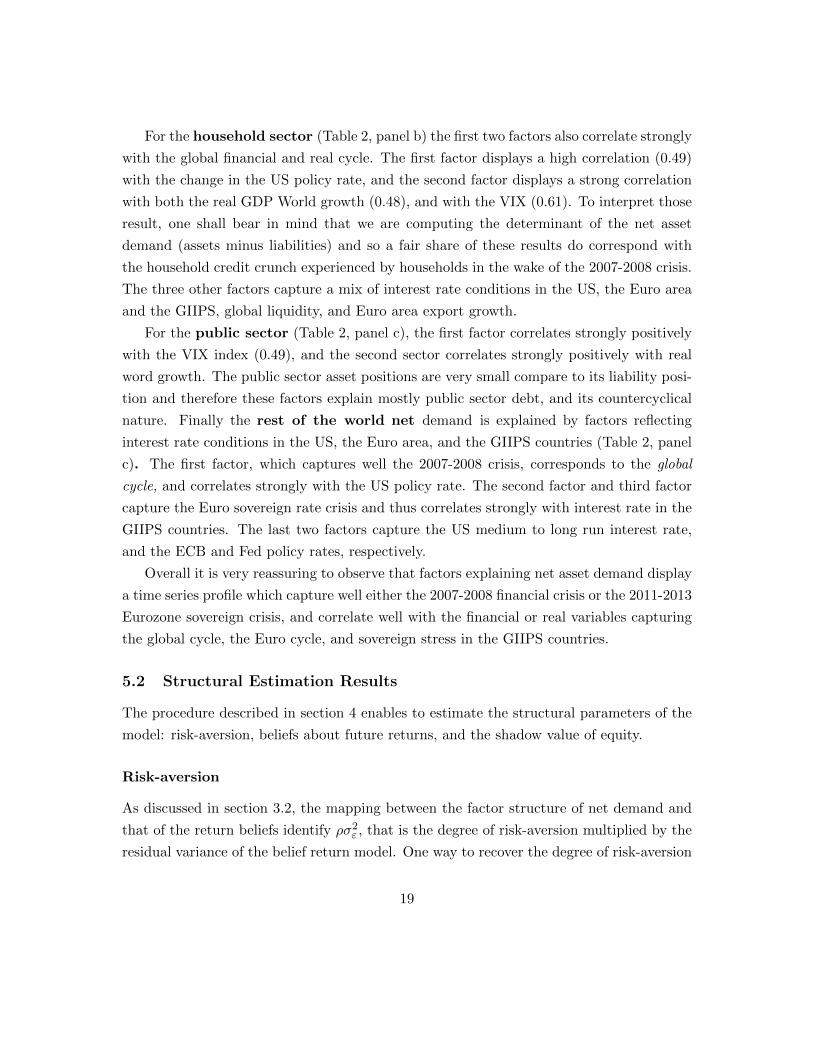
For the household sector (Table 2, panel b) the first two factors also correlate strongly

with the global financial and real cycle. The first factor displays a high correlation (0.49)

with the change in the US policy rate, and the second factor displays a strong correlation

with both the real GDP World growth (0.48), and with the VIX (0.61). To interpret those

result, one shall bear in mind that we are computing the determinant of the net asset

demand (assets minus liabilities) and so a fair share of these results do correspond with

the household credit crunch experienced by households in the wake of the 2007-2008 crisis.

The three other factors capture a mix of interest rate conditions in the US, the Euro area

and the GIIPS, global liquidity, and Euro area export growth.

For the public sector (Table 2, panel c), the first factor correlates strongly positively

with the VIX index (0.49), and the second sector correlates strongly positively with real

word growth. The public sector asset positions are very small compare to its liability posi-

tion and therefore these factors explain mostly public sector debt, and its countercyclical

nature. Finally the rest of the world net demand is explained by factors reflecting

interest rate conditions in the US, the Euro area, and the GIIPS countries (Table 2, panel

c). The first factor, which captures well the 2007-2008 crisis, corresponds to the global

cycle, and correlates strongly with the US policy rate. The second factor and third factor

capture the Euro sovereign rate crisis and thus correlates strongly with interest rate in the

GIIPS countries. The last two factors capture the US medium to long run interest rate,

and the ECB and Fed policy rates, respectively.

Overall it is very reassuring to observe that factors explaining net asset demand display

a time series profile which capture well either the 2007-2008 financial crisis or the 2011-2013

Eurozone sovereign crisis, and correlate well with the financial or real variables capturing

the global cycle, the Euro cycle, and sovereign stress in the GIIPS countries.

5.2 Structural Estimation Results

The procedure described in section 4 enables to estimate the structural parameters of the

model: risk-aversion, beliefs about future returns, and the shadow value of equity.

Risk-aversion

As discussed in section 3.2, the mapping between the factor structure of net demand and

that of the return beliefs identify ρσ2ε , that is the degree of risk-aversion multiplied by the

residual variance of the belief return model. One way to recover the degree of risk-aversion

19

is by matching the overall variance of return beliefs to the variance of ex-post returns.

Table 2, upper panel, report risk-aversion estimates, one by sector, obtained by matching

variances. This approach generates estimates, which tend to be on the high side, ranging

from 8.9 to 21.7, depending on the institutional sector, but which are not uncommon in

the finance literature.6 The ordering of risk-aversion between sectors is sensible with a

higher estimated risk-aversion in financial sectors subject to capital requirement (banks,

insurance) than for the mutual funds sector or the corporate sector.

While imposing the matching of belief returns to ex-post returns is a way to discipline

belief formation, one cannot rule out that beliefs are substantially more volatile than

ex-post returns. Moreover by letting the variance of return beliefs to be a multiple of

the variance of ex-post returns (Table 2, bottom three panels), we estimate risk-aversion

parameters that are substantially smaller. The estimation of return beliefs presented in the

next section are obtained by matching the variance of return beliefs with that of ex-post

returns.7

Return Beliefs

The estimated factor model for return beliefs, described in Section 3.1, yields for each

sector and each instrument, a one-quarter-ahead return forecast. Figure 3 and Figure 5

plot alongside the time series of realized ex-post returns the time series of corresponding

return beliefs, the 95th percent confidence forecast interval band, for the financial sectors

and the real sectors, and for each of the following financial instruments: Bonds (Short-

Term and Long-Term), Stocks (Listed and Unlisted), Mutual Fund Shares (Money Market

and Non-Money Market). The R-square of an OLS regression of ex-post returns on ex-ante

return beliefs and a constant is reported on the right-hand upper corner of each plot.

In many cases, the ex-ante return beliefs predict well ex-post returns. The corporate

sector ex-ante return beliefs explain 31 percent of the variance of ex-post stock returns. The

household sector ex-ante return beliefs explain 35 percent of the variance of the Non Money

Market Mutual Funds ex-post returns. In both cases, the time series of return belief tracks

very well the asset crash of 2007-2008, and the subsequent rebound. Other good predicting

performance include the prediction of unlisted stock returns by the banking sector and the

household sector, the prediction of short-term bonds return by the insurance sector, the

6Ang (2014) and Ait Sahalia & Lo (2000)7Estimations based on alternative calibration of risk-aversion are available from the authors.

20

prediction of the return to mutual funds by the corporate sector, the household sector, and

the mutual fund sector itself.

In several instances however, the model either does not predict ex-post return or more

puzzlingly its predictions negatively correlate with ex-post returns. We shall notice that

this feature is mostly driven by the 2007-2008 crisis. A potential explanation is that several

institutional sectors during that period had to increase their purchases of assets even if

their returns were declining. Since beliefs are implicitly derived from net demands, those

counter-cyclical purchases can drive the negative correlation between return beliefs and

ex-post returns. This is the case for the banking sector which hoarded short term liquid

assets during the crisis, for the public sector who bought large stock shares to recaptilize

the banking sector and the automobile sector during the crisis, and for the insurance sector

which increased considerably its asset holdings during the crisis (Heipertz et al. 2016).

Figure 4 and 6 illustrate the dispersion of beliefs between the three financial sectors

(banking, insurance, mutual funds), and between the three real domestic sectors (corporate,

household, public). Overall, while there is substantial disagreement in beliefs at each point

in time, the return beliefs of the banking sector and the mutual fund sectors display a strong

comovement. The correlation between the return beliefs of the banking sector and those

of the mutual fund sectors are high for most financial instruments: listed stocks (0.54),

unlisted stocks (0.46), non money-market mutual fund share (0.34), short-term debt (0.40).

There are however episodes in which the return beliefs differ substantially. For example,

the mutual fund sector exhibited much more pessimistic beliefs during the 2007-2008 crisis

about the return to stocks and to debt securities, while the banking sector became more

pessimist on the returns to stocks and mutual fund shares during the sovereign crisis of

2011-2012. One interpretation is that the bank bailout of 2007-2008 avoided the need for

banks to engage in massive fire-sales (with deep discount prices), while the mutual fund

sector faced large withdrawals from customers and had to engage in such fire-sales. On

the opposite, banks were suffering from significant liquidity or solvency stress during the

sovereign debt crisis, due to their exposure to GIIPS debt, and therefore faced a pressure

to sell-off rapidly other assets that the mutual fund sector did not experience then.

The comparison of beliefs among the three real sectors reveal a sharp contrast between

the belief returns of the corporate and household that typically comove, and that of the

public sector that often displays counter-cyclical beliefs, and especially so during the 2007-

2008 crisis. This is consistent with the role played by government in providing bailout and

in the debt financing of large public sector deficits during the crisis.

21

Value of Equity

Figure 7 plots the shadow value of equity for each of the sector of the economy. For the

corporate and banking sector, the shadow value of issuing more equity declined during the

crisis and rebounded afterwards. The insurance sector value of equity increased sharply in

the aftermath of the crisis in line with its increase in net asset holdings. The public sector

value of equity declined sharply in the crisis and post-crisis period, a period during which

public debt increased strongly.

5.3 Networks, and Shock Propagation

Following section 2.4, the estimated net asset demand model yields both a network of

assets and a network of institutions. We focus here on the network formed by the tradable

instruments: Bonds (Short-Term and Long-Term), Stocks (Listed and Unlisted), Mutual

Fund Shares (Money Market and Non-Money Market). Figure 8 represents the network of

financial instruments for two dates: (i) the first quarter of 2008, that is before the financial

crisis; (2) the recent period (2015.Q1). In the pre-crisis era, the demand for equity and non

money-market mutual fund share were the most affected by changes in the returns to other

assets. By contrast, in the post-crisis era, the demand for long-term debt became the most

affected demand, reflecting both increased issuances of corporate debt in a low-interest

rate environment, and increased loading of government securities in balance-sheets, and

especially so in the banking and insurance sector.

A convenient way to illustrate the importance of network propagation is to contrast the

partial equilibrium effect of a shock, which by construction abstracts from any networks

effects, to the general equilibrium effect which incorporates the full array of network effects

. In order to do this comparison, we fist derive the partial equilibrium effect of a shock to

the equity of sector k.

Proposition 4. The partial equilibrium effect of a shock to sector k’s equity Ekt on net

demands is given by

∂∆kt

∂Ekt= Σ−1

k

(1′Σ−1

k 1)−1

1, and∂∆k′t

∂Ekt= 0 ∀k′ 6= k,

where Σk is the J × J variance-covariance matrix of return beliefs of sector k. The partial

equilibrium effect of equity on net demand is time independent.

22

Note that while the partial equilibrium impact of a shock on equity is constant, the

general equilibrium effect varies over time along with the price sensitivity of net demands to

changes in log returns which characterize the time-varying network of financial instruments

(see section 2.4).

Table 10 shows the partial and general equilibrium effect of a shock to the equity of

the banking sector. The shock corresponds to one unit increase in the capital base of the

banking sector. Table 10, panel (b) shows the effects for 2015.Q1, a period of tranquil times

and Table 10, panel (a) for 2008.Q4, a period of crisis time.

By comparing the first and second column of table 10, panel (b), we can contrast the

partial and general equilibrium effects of the shock the banking sector itself. In the partial

equilibrium effect the one-unit increase in equity finance a one-unit increase in net assets

distributed more of less equally across the three asset classes (stocks, bonds, mutual funds).

In general equilibrium however price effects reduces the increase in net asset demand for

all asset classes and the total net demand for assets in the banking sector ends up being

30 percent smaller than in partial equilibrium.

For the other sectors, only the general equilibrium effects arise and they appear to be

very heterogeneous across sectors. Following a one-unit shock to equity in the banking

sector, the corporate sector also increase its net asset demands (+0.58) but all the other

sectors experience a decrease in net asset demand. The reduction is small for the household

sector (-0.045) but with substantial rebalancing in net asset position away from listed

stocks, short-debt debt, and non money market mutual funds, and towards unlisted stocks,

long-term debt, and money market funds. The reduction in net asset demand is much larger

for the insurance sector with a reduction of -0.45 in total net asset demand and a reduction

in the net asset demand for all asset classes.

The re-balancing of net demand between the banking sector and the insurance sector

is quiet remarkable as it is closely related with what happened in the aftermath 2007-2008,

that is a retrenchment of the banking sector net asset holdings following severe capital

losses, and an expansion of the insurance sector net asset holdings(Heipertz et al. 2016).

The last column displays the change in log returns and indicates a marked dispersion in

returns between assets with a decline in the returns of listed stocks, short-term debt, and

non money-market mutual fund shares while the returns of other instruments increased.

Table 10, panel (a) explores network effects that unfolded in the midst of the 2007-2008

financial crisis (2008.Q4). The increase in net asset demand by the banking and corporate

sectors was, back then, considerably lower (0.5 and 0.215) than in “tranquil times”. By

23

contrast, all other sectors experienced a decline in their net asset demand. That decline was

more marked than in “tranquil times” for households (-0.08), but less so for the insurance

sector (-0.26). Meanwhile, the Rest of the World increased net asset holdings relative to

“tranquil times”.

Overall, it turns out that the network effects derived from the general equilibrium

analysis are (i) sizeable in some sectors, of a magnitude comparable to the sector where

the shock originated; (ii) very contrasted across sector, vindicating the phenomonon of

large net demand shifts across sectors such as between the banking and the insurance

sector.

6 Conclusion

This paper develops a novel methodology to estimate the key parameters of a general

equilibrium model of net asset trade by using the factor structure of net asset demand.

The structure of net asset demand is well explained by a number of factors that strongly

correlate with macro-variables capturing the global cycle or the Eurozone cycle. The

estimated model for return beliefs predicts well ex-post returns for many sectors and many

financial instruments. The cased of predictions failure can be related to special episodes

such as the 2007-2008 crisis during which some sectors (insurance, public sector) displayed

a counter-cyclical behavior increasing net holdings of assets whose return were declining.

The estimated model yields both a network of financial instrument and a networks of

institutions. The transmission of shocks in the networks, through price externalities, reveal

network effects which are large and strongly heterogeneous across sectors. Extending the

model to account for regulatory constraints in order to simulate regulatory changes, and

re-estimating the model on individual institutions are the next steps on the agenda.

24

References

Acemoglu, D., Ozdaglar, A. & Tahbaz-Salehi, A. (2015), ‘Systemic risk and stability in

financial networks’, American Economic Review 105.

Ait Sahalia, Y. & Lo, A. W. (2000), ‘Nonparametric risk management and implied risk

aversion’, Journal of Econometrics 94.

Ang, A. (2014), ‘Asset management: A systematic approach to factor investing’, OUP

Catalogue, Oxford University Press .

Berrada, T. (2006), ‘Incomplete information, heterogeneity and asset pricing’, Journal of

Financial Econometrics 4.

Eisenberg, L. & Noe, T. H. (2001), ‘Systemic risk in financial systems’, Management Science

47.

Elliott, M., Golub, B. & Jackson, M. O. (2014), ‘Financial networks and contagion’, Amer-

ican Economic Review 104.

Gandhi, A. & Serrano-Padial, R. (2015), ‘Does belief heterogeneity explain asset prices:

The case of the longshot bias’, Review of Economic Studies 82.

Goyal, S. & Vega-Redondo, F. (2005), ‘Network formation and social coordination’, Games

and Economic Behavior 50.

Greenwood, R., Landier, A. & Thesmar, D. (2015), ‘Vulnerable banks’, Journal of Finan-

cial Economics 115.

Heipertz, J., Ranciere, R. & Valla, N. (2016), ‘Domestic and international sectoral portfo-

lios: Network structure and balance sheet effects’, mimeo .

Jackson, M. & Watts, A. (2002), ‘The evolution of social and economic networks’, Journal

of Economic Theory 106.

Koijen, R. S. & Yogo, M. (2016), ‘An equilibrium model of institutional demand and asset

prices’, NBER Working Paper No. 21749 .

Mas-Colell, A., Whinston, M. D., Green, J. R. et al. (1995), Microeconomic theory, Vol. 1,

Oxford university press New York.

25

Miranda-Agrippino, S. & Rey, H. (2015), ‘World asset markets and the global financial

cycle’, NBER Working Paper No. 21722 .

Wu, J. C. & Xia, F. D. (2016), ‘Measuring the macroeconomic impact of monetary policy

at the zero lower bound’, Journal of Money, Credit and Banking 48.

26

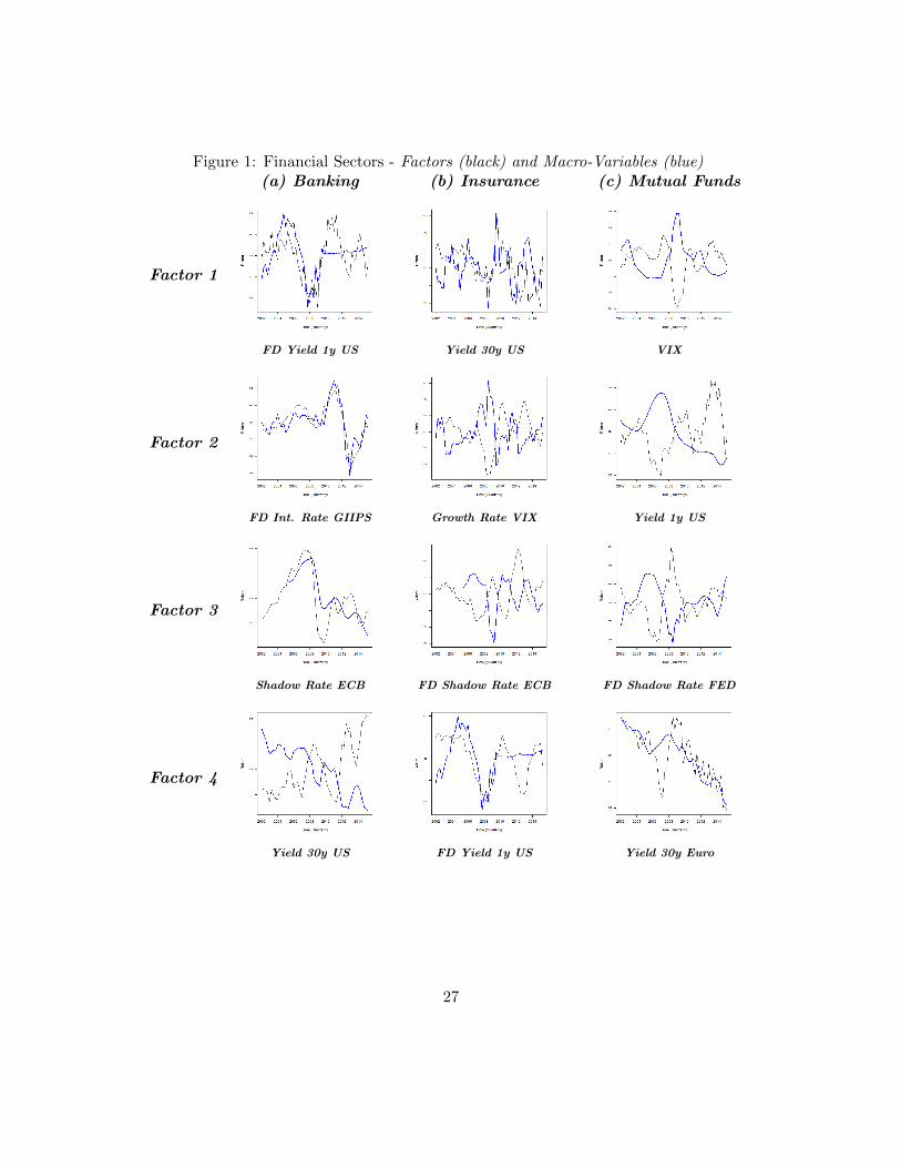
Figure 1: Financial Sectors - Factors (black) and Macro-Variables (blue)(a) Banking (b) Insurance (c) Mutual Funds

Factor 1

FD Yield 1y US Yield 30y US VIX

Factor 2

FD Int. Rate GIIPS Growth Rate VIX Yield 1y US

Factor 3

Shadow Rate ECB FD Shadow Rate ECB FD Shadow Rate FED

Factor 4

Yield 30y US FD Yield 1y US Yield 30y Euro

27

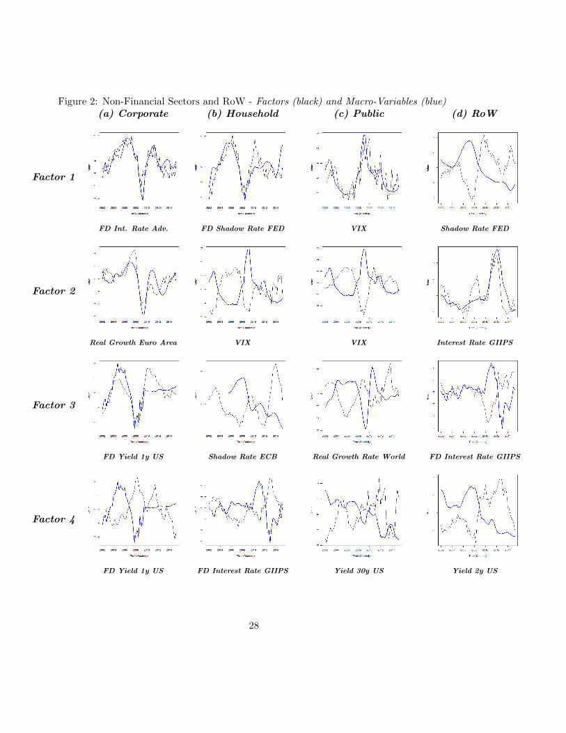
Figure 2: Non-Financial Sectors and RoW - Factors (black) and Macro-Variables (blue)(a) Corporate (b) Household (c) Public (d) RoW

Factor 1

FD Int. Rate Adv. FD Shadow Rate FED VIX Shadow Rate FED

Factor 2

Real Growth Euro Area VIX VIX Interest Rate GIIPS

Factor 3

FD Yield 1y US Shadow Rate ECB Real Growth Rate World FD Interest Rate GIIPS

Factor 4

FD Yield 1y US FD Interest Rate GIIPS Yield 30y US Yield 2y US

28

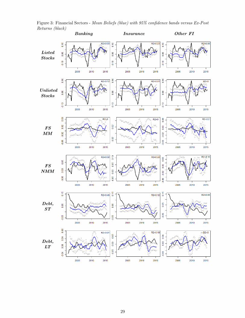
Figure 3: Financial Sectors - Mean Beliefs (blue) with 95% confidence bands versus Ex-PostReturns (black)

Banking Insurance Other FI

ListedStocks

UnlistedStocks

FSMM

FSNMM

Debt,ST

Debt,LT

29

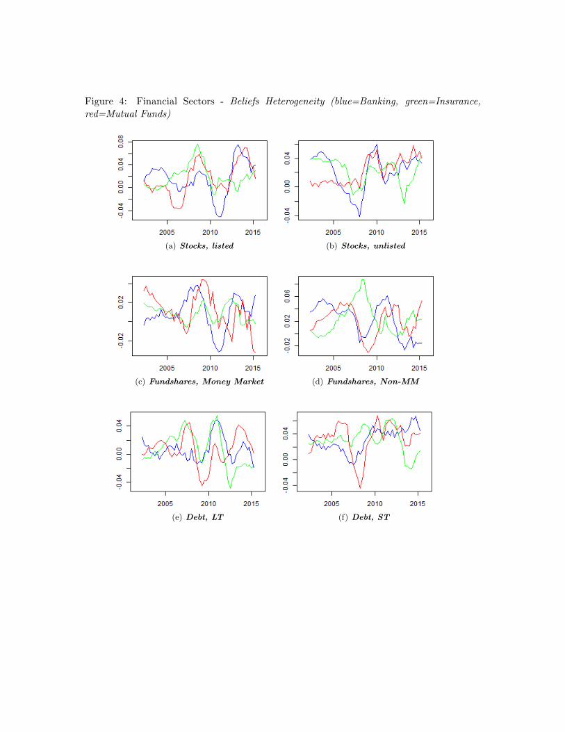
Figure 4: Financial Sectors - Beliefs Heterogeneity (blue=Banking, green=Insurance,red=Mutual Funds)

(a) Stocks, listed (b) Stocks, unlisted

(c) Fundshares, Money Market (d) Fundshares, Non-MM

(e) Debt, LT (f) Debt, ST

30

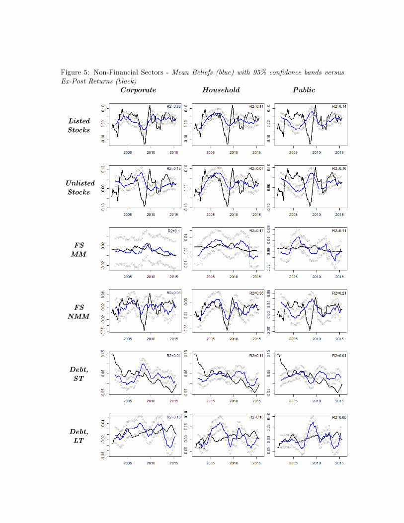
Figure 5: Non-Financial Sectors - Mean Beliefs (blue) with 95% confidence bands versusEx-Post Returns (black)

Corporate Household Public

ListedStocks

UnlistedStocks

FSMM

FSNMM

Debt,ST

Debt,LT

31

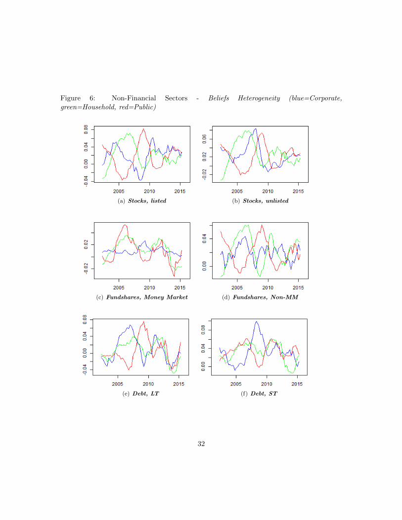
Figure 6: Non-Financial Sectors - Beliefs Heterogeneity (blue=Corporate,green=Household, red=Public)

(a) Stocks, listed (b) Stocks, unlisted

(c) Fundshares, Money Market (d) Fundshares, Non-MM

(e) Debt, LT (f) Debt, ST

32

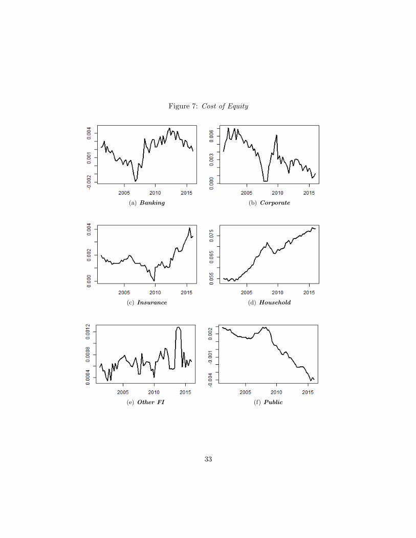
Figure 7: Cost of Equity

(a) Banking (b) Corporate

(c) Insurance (d) Household

(e) Other FI (f) Public

33

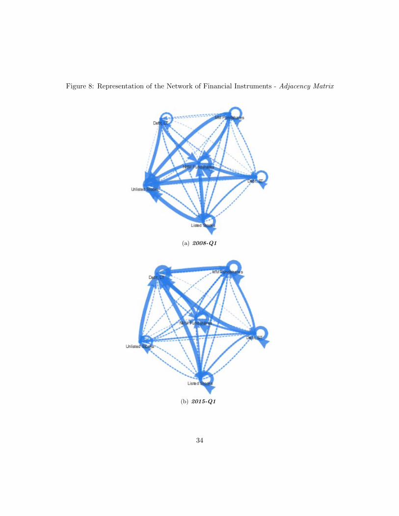
Figure 8: Representation of the Network of Financial Instruments - Adjacency Matrix

(a) 2008-Q1

(b) 2015-Q1

34

Table 1: Macro-Variables and SourcesMacro-Variable Source Comments

ECB and FED Shadow Rate Wu and Xia (2016)

Interest Rate Adv. Economies IFS Average of yields on governmentsecurities of Belgium, France,Netherlands, Germany, Italy, Japan andthe US

Interest Rate GIIPS IFS Average of Yields on governmentsecurities of Greece, Ireland, Italy,Portugal and Spain (GIIPS)

Liquidity Growth World IFS Q-on-q growth rate of the sum ofmonetary aggregates M2 of the Euroarea, Japan, the United Kingdom andthe US

S&P 500 VIX CBOE Implied volatility of S&P 500 indexoptions

Real Export Growth Euro area IFSReal Export Growth World IFSReal GDP Growth Euro area IFSReal GDP Growth World IFSReal Import Growth World IFSReal Trade Growth World IFSYield Cuve US JP Morgan Mid yield curveYields Cuve Euro area JP Morgan Mid yield curve Germany

35

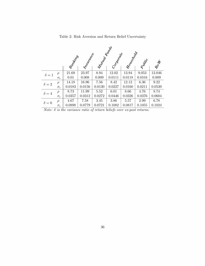
Table 2: Risk Aversion and Return Belief Uncertainty

Banking

Insurance

MutualFunds

Corporate

Household

Public

RoW

δ = 1ρ 21.69 23.97 8.94 12.02 13.94 9.053 12.046σε 0.01 0.008 0.009 0.0111 0.0118 0.0104 0.009

δ = 2ρ 14.18 16.96 7.56 8.42 12.12 6.36 9.22σε 0.0183 0.0156 0.0130 0.0227 0.0160 0.0211 0.0539

δ = 4ρ 8.73 11.99 5.52 6.01 8.66 4.76 8.74σε 0.0357 0.0312 0.0272 0.0446 0.0326 0.0376 0.0604

δ = 6ρ 4.67 7.58 3.45 3.86 5.57 2.99 6.78σε 0.0898 0.0779 0.0721 0.1082 0.0817 0.1055 0.1024

Note: δ is the variance ratio of return beliefs over ex-post returns.

36

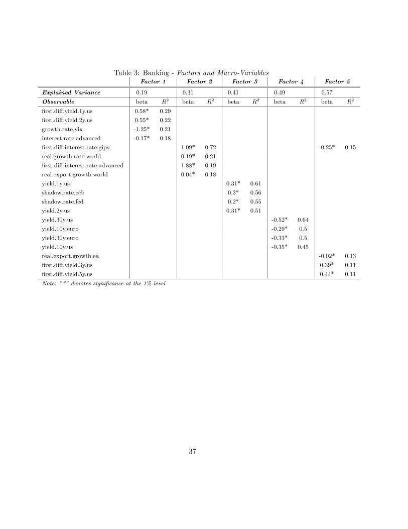
Table 3: Banking - Factors and Macro-VariablesFactor 1 Factor 2 Factor 3 Factor 4 Factor 5

Explained Variance 0.19 0.31 0.41 0.49 0.57

Observable beta R2 beta R2 beta R2 beta R2 beta R2

first.diff.yield.1y.us 0.58* 0.29


growth.rate.vix -1.25* 0.21

interest.rate.advanced -0.17* 0.18

first.diff.interest.rate.gips 1.09* 0.72 -0.25* 0.15

real.growth.rate.world 0.19* 0.21

first.diff.interest.rate.advanced 1.88* 0.19

real.export.growth.world 0.04* 0.18

yield.1y.us 0.31* 0.61

shadow.rate.ecb 0.3* 0.56

shadow.rate.fed 0.2* 0.55

yield.2y.us 0.31* 0.51

yield.30y.us -0.52* 0.64

yield.10y.euro -0.29* 0.5


yield.10y.us -0.35* 0.45

real.export.growth.ea -0.02* 0.13



Note: ”*” denotes significance at the 1% level

37

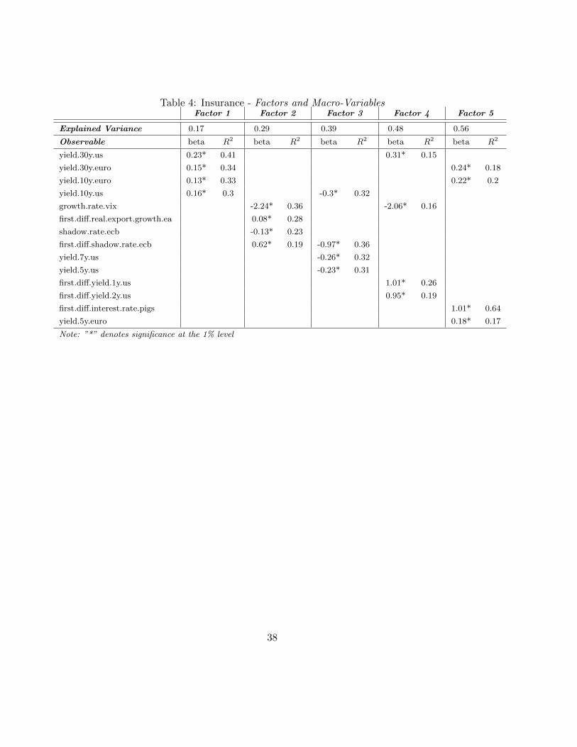
Table 4: Insurance - Factors and Macro-VariablesFactor 1 Factor 2 Factor 3 Factor 4 Factor 5



yield.30y.us 0.23* 0.41 0.31* 0.15

yield.30y.euro 0.15* 0.34 0.24* 0.18

yield.10y.euro 0.13* 0.33 0.22* 0.2

yield.10y.us 0.16* 0.3 -0.3* 0.32

growth.rate.vix -2.24* 0.36 -2.06* 0.16

first.diff.real.export.growth.ea 0.08* 0.28

shadow.rate.ecb -0.13* 0.23

first.diff.shadow.rate.ecb 0.62* 0.19 -0.97* 0.36

yield.7y.us -0.26* 0.32

yield.5y.us -0.23* 0.31



first.diff.interest.rate.pigs 1.01* 0.64

yield.5y.euro 0.18* 0.17


38

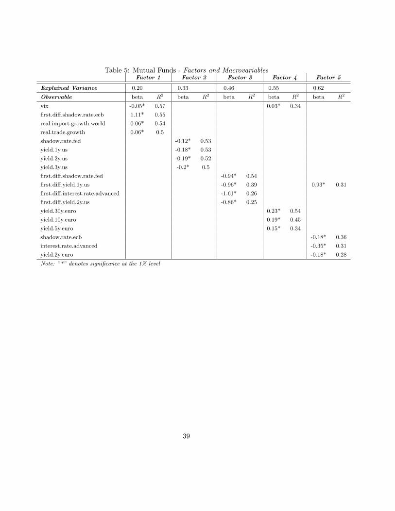
Table 5: Mutual Funds - Factors and MacrovariablesFactor 1 Factor 2 Factor 3 Factor 4 Factor 5



vix -0.05* 0.57 0.03* 0.34

first.diff.shadow.rate.ecb 1.11* 0.55

real.import.growth.world 0.06* 0.54

real.trade.growth 0.06* 0.5

shadow.rate.fed -0.12* 0.53

yield.1y.us -0.18* 0.53

yield.2y.us -0.19* 0.52

yield.3y.us -0.2* 0.5

first.diff.shadow.rate.fed -0.94* 0.54

first.diff.yield.1y.us -0.96* 0.39 0.93* 0.31

first.diff.interest.rate.advanced -1.61* 0.26

first.diff.yield.2y.us -0.86* 0.25








39

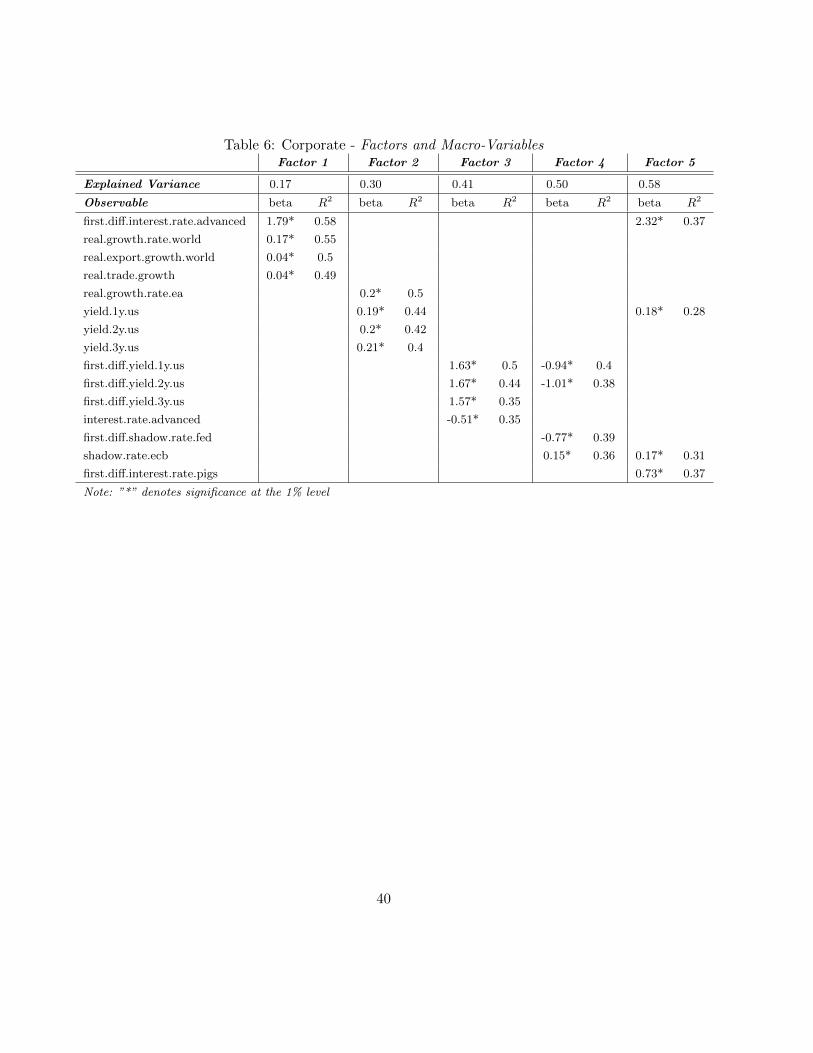
Table 6: Corporate - Factors and Macro-VariablesFactor 1 Factor 2 Factor 3 Factor 4 Factor 5



first.diff.interest.rate.advanced 1.79* 0.58 2.32* 0.37

real.growth.rate.world 0.17* 0.55

real.export.growth.world 0.04* 0.5

real.trade.growth 0.04* 0.49

real.growth.rate.ea 0.2* 0.5

yield.1y.us 0.19* 0.44 0.18* 0.28

yield.2y.us 0.2* 0.42

yield.3y.us 0.21* 0.4

first.diff.yield.1y.us 1.63* 0.5 -0.94* 0.4

first.diff.yield.2y.us 1.67* 0.44 -1.01* 0.38




shadow.rate.ecb 0.15* 0.36 0.17* 0.31

first.diff.interest.rate.pigs 0.73* 0.37


40

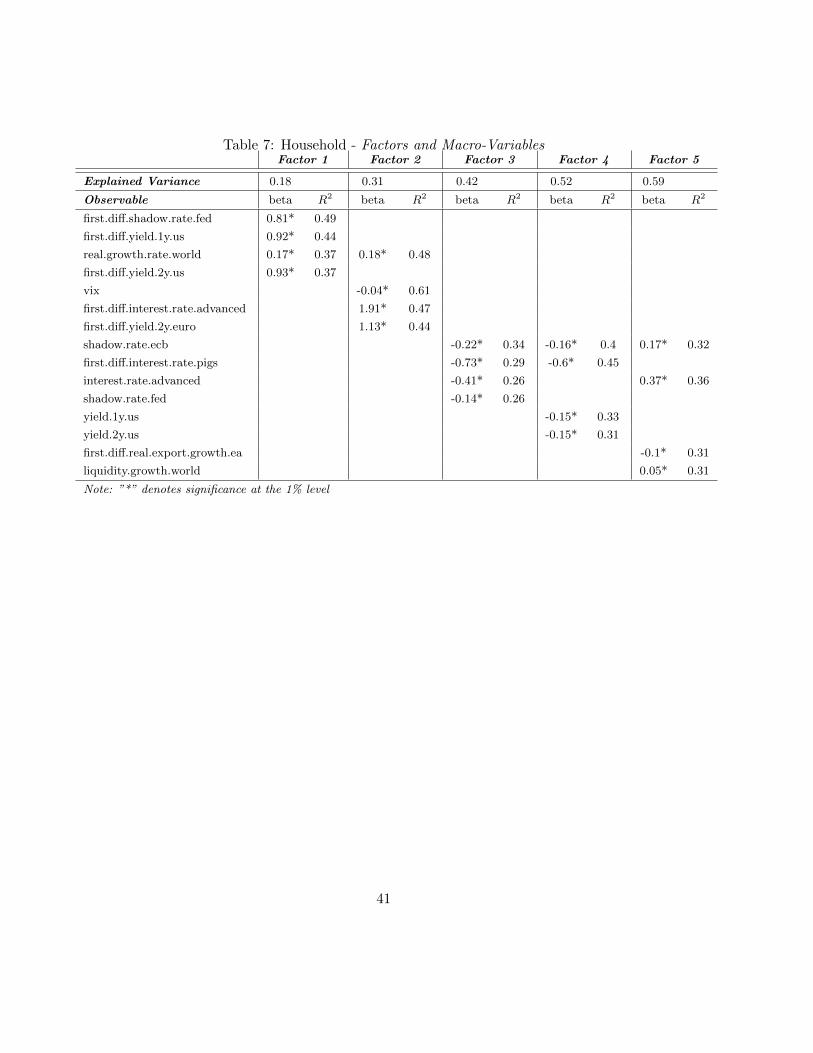
Table 7: Household - Factors and Macro-VariablesFactor 1 Factor 2 Factor 3 Factor 4 Factor 5



first.diff.shadow.rate.fed 0.81* 0.49


real.growth.rate.world 0.17* 0.37 0.18* 0.48


vix -0.04* 0.61

first.diff.interest.rate.advanced 1.91* 0.47

first.diff.yield.2y.euro 1.13* 0.44

shadow.rate.ecb -0.22* 0.34 -0.16* 0.4 0.17* 0.32

first.diff.interest.rate.pigs -0.73* 0.29 -0.6* 0.45

interest.rate.advanced -0.41* 0.26 0.37* 0.36

shadow.rate.fed -0.14* 0.26

yield.1y.us -0.15* 0.33

yield.2y.us -0.15* 0.31

first.diff.real.export.growth.ea -0.1* 0.31

liquidity.growth.world 0.05* 0.31


41

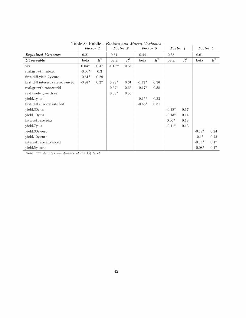
Table 8: Public - Factors and Macro-VariablesFactor 1 Factor 2 Factor 3 Factor 4 Factor 5



vix 0.03* 0.47 -0.07* 0.64

real.growth.rate.ea -0.09* 0.3

first.diff.yield.2y.euro -0.61* 0.29

first.diff.interest.rate.advanced -0.97* 0.27 3.29* 0.61 -1.77* 0.36

real.growth.rate.world 0.32* 0.63 -0.17* 0.38

real.trade.growth.ea 0.08* 0.56

yield.1y.us -0.15* 0.33


yield.30y.us -0.18* 0.17

yield.10y.us -0.13* 0.14

interest.rate.pigs 0.06* 0.13

yield.7y.us -0.11* 0.13

yield.30y.euro -0.12* 0.24





42

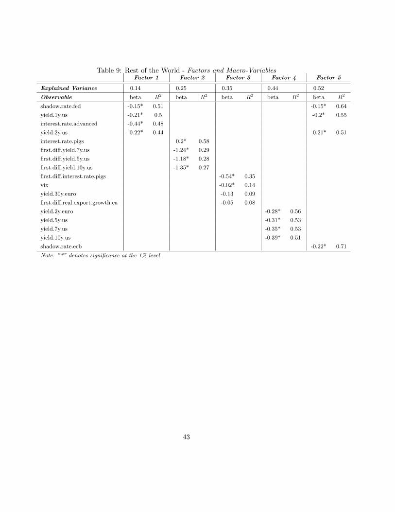
Table 9: Rest of the World - Factors and Macro-VariablesFactor 1 Factor 2 Factor 3 Factor 4 Factor 5



shadow.rate.fed -0.15* 0.51 -0.15* 0.64

yield.1y.us -0.21* 0.5 -0.2* 0.55


yield.2y.us -0.22* 0.44 -0.21* 0.51

interest.rate.pigs 0.2* 0.58




first.diff.interest.rate.pigs -0.54* 0.35

vix -0.02* 0.14

yield.30y.euro -0.13 0.09

first.diff.real.export.growth.ea -0.05 0.08


yield.5y.us -0.31* 0.53

yield.7y.us -0.35* 0.53

yield.10y.us -0.39* 0.51



43

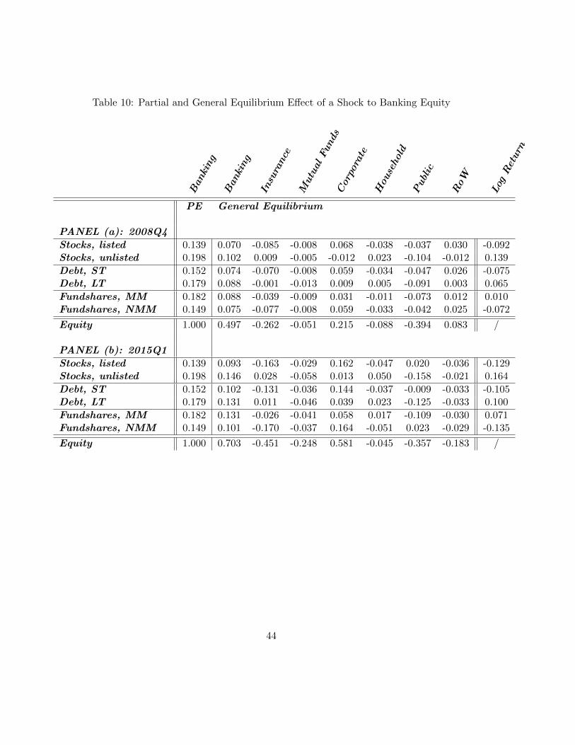
Table 10: Partial and General Equilibrium Effect of a Shock to Banking Equity

Banking

Banking

Insurance

MutualFunds

Corporate

Household

Public

RoW

Log

Return

PE General Equilibrium

PANEL (a): 2008Q4

Stocks, listed 0.139 0.070 -0.085 -0.008 0.068 -0.038 -0.037 0.030 -0.092Stocks, unlisted 0.198 0.102 0.009 -0.005 -0.012 0.023 -0.104 -0.012 0.139

Debt, ST 0.152 0.074 -0.070 -0.008 0.059 -0.034 -0.047 0.026 -0.075Debt, LT 0.179 0.088 -0.001 -0.013 0.009 0.005 -0.091 0.003 0.065

Fundshares, MM 0.182 0.088 -0.039 -0.009 0.031 -0.011 -0.073 0.012 0.010Fundshares, NMM 0.149 0.075 -0.077 -0.008 0.059 -0.033 -0.042 0.025 -0.072

Equity 1.000 0.497 -0.262 -0.051 0.215 -0.088 -0.394 0.083 /

PANEL (b): 2015Q1

Stocks, listed 0.139 0.093 -0.163 -0.029 0.162 -0.047 0.020 -0.036 -0.129Stocks, unlisted 0.198 0.146 0.028 -0.058 0.013 0.050 -0.158 -0.021 0.164

Debt, ST 0.152 0.102 -0.131 -0.036 0.144 -0.037 -0.009 -0.033 -0.105Debt, LT 0.179 0.131 0.011 -0.046 0.039 0.023 -0.125 -0.033 0.100

Fundshares, MM 0.182 0.131 -0.026 -0.041 0.058 0.017 -0.109 -0.030 0.071Fundshares, NMM 0.149 0.101 -0.170 -0.037 0.164 -0.051 0.023 -0.029 -0.135

Equity 1.000 0.703 -0.451 -0.248 0.581 -0.045 -0.357 -0.183 /

44

A Theory – Proofs

Proposition 2. (Existence of an Equilibrium) There exists a price vector p∗t ∈ RJ such

that∑N

i=1 ∆it(p∗t ) = Et(p

∗t ).

Proof. For clarity of exposition and without loss of generality, we omit the subscript t in the

notations for this proof. Write ∆(p) =∑N

i=1 ∆i(p1, p2, . . . , pJ) − E(p1, p2, . . . , pJ). Throughout

the paper and following the conventions of the asset portfolio allocation literature, ∆(p) is the

value of net demand. We thus write z(p) the net demand in units of financial instruments, and

thus ∆(p) = p z(p) is the term by term product of the price vector and the net demand vector

in units.

An equilibrium price vector is a J-vector p such that z(p) = 0.

Following Mas-Colell, Whinston, Green et al. (1995), we need to show that the aggregate net

demand curve p ∈ RJ+∗ 7→ z(p) ∈ RJ satisfies the following properties:

1. z(·) is continuous.

2. z(·) is homogenous of degree zero.

3. p · z(p) = 0 for all p, i.e. Walras law is satisfied.

4. There is an s > 0 such that zj(p) > −s for all financial instruments j = 1, 2, . . . , J and for

all price vectors p.

5. If pn → p, where p 6= 0 and pj = 0 for some j, then

max z1(pn), . . . , zJ(pn) → ∞

The continuity of z(·) over RJ+∗ is established as follows. First, the variance-covariance matrix Σ

is a continuous function of the price vector of RJ+∗ . Following the assumption of section 2.1, it

satisfies det Σ(p) 6= 0 for all p ∈ RJ as a positive definite symmetric matrix. Thus the inverse

Σ−1(p) is a continuous function of prices. Second, the mean return µ is a continuous function of

p. Third, the cost of equity, a rational function of Σ−1 and µ with no root in the denominator, is

also a continuous function of p.

The homogeneity of z(·) is established by writing the expression for z(p), where p includes the

price of shares pj(i):

z(p) =

N∑i=1

diag(1

p)

[1

ρΣ−1i (µi − ηi1)

], (26)

45

where is the term by term vector multiplication. And ηi = (1′Σ−1µ − ρpj(i)Ξi)/(1′Σ−11).

Multiplying all prices by a constant λ > 0 multiplies the mean returns µi by 1/λ, multiplies the

inverse of the variance-covariance matrix Σ−1i by a constant λ

2, and the cost of equity by λ. Given

the lead factor diag( 1p), the net demand z(λp) is unchanged, and z(λp) = z(p).

Walras law follows from the sum of the funding constraints, as

p · z(p) =

J∑j=1

N∑i=1

(∆ij(p)− 1(j(i) = j)Ei(p)) = 0. (27)

On point 4.: the existence of a lower bound for net demands z(p) follows from the funding

constraint (1). Indeed, assume that there is no s such that zj(p) > −s for all financial instru-

ments j = 1, 2, . . . , J and for all price vectors p. Then we can build a sequence (sk,pk) such that

sk → ∞ as k → ∞, and for each k, there is a j′(k) in 1, 2, . . . , J for which −sk > zj′(k)(pk).

Given the funding constraint, this implies that there will be a similar sequence for which demand

will go to infinity. Formally, there is a sequence (σk,πk) such that σk → ∞ as k → ∞, and for

each k, there is a j′′(k) in 1, 2, . . . , J for which zj′′(k)(πk) > σk. This, however, implies that the

variance of the firm’s portfolio diverges to infinity as k → ∞, which cannot be a solution to the

optimization program (2).

The last point follows from the fact that if asset j’s return diverges to infinity, µj → ∞ and

therefore according to equation (3), one of the components of net demand will diverge to infinity.

Given that properties 1–5 are satisfied, an equilibrium price vector p∗ exists with z(p∗) = 0.

B Data Appendix

B.1 Estimation of Returns from Sectoral Accounts

There are two challenges for deriving returns on financial instrument categories from sectoral

account data.

1. Returns are specific to the sectoral investment position. The sectoral accounts provide

information on aggregates of financial instruments of the same type. No information exists on

sectoral portfolio allocations across financial instruments of the same type. Returns realized

on financial instruments of the same type therefore vary across sector, due to differences in

inter-type allocations.

2. Pay-offs are recorded only at the sectoral level as income received or payed in the income

46

accounts. Therefore dividends, interest payments and investment income cannot be directly

attributed to financial instruments.

We use the variation of investment positions across sectors and financial instruments, the variation

of valuation changes across sectors and financial instruments and the variation of income received

or payed across sectors to estimate subsequently: (i) the return due to valuation changes and (ii)

the return due to payoffs. Financial instruments are indexed by j = 1, ..., J and sectors are indexed

by i = 1, ..., I. Furthermore, PDt and P S

t are matrices of size I × J that collect the demand and

supply by I sectors for J financial instruments, respectively. The rate of return due to valuation

changes is denoted by gjt+1 and the rate of return due to payoffs is denoted by πjt+1.

Assumption 1. The return on asset j demanded or supplied by sector i have an asset-specific

component and a component specific to the financial position f ∈ D,S of sector i.

πfijt+1 = πjt+1 + ufit+1, f ∈ D,S (28)

gfijt+1 = gjt+1 + vfit+1, f ∈ D,S (29)

where D denotes the demand/asset side of the balance-sheet and S the supply/liability side of the

balance-sheet. We assume that the component specific to the financial position f ∈ D,S of sector

i is iid distributed with mean zero.

Collecting the pay-offs and valuation gains received or payed on J assets by I sectors in the

matricesΠft and Gf

t of dimension I × J , respectively, Assumption 1 implies that the return in

amount of currency units realized can be written in matrix notation as

Πft = P f

t diag (πt+1) + diag(uft+1

)P ft , f ∈ D,S (30)

Gft = P f

t diag(gt+1

)+ diag

(vft+1

)P ft , f ∈ D,S (31)

As argued above, not all returns realized by sectors on financial instruments are fully observable.

For example, only the sum of interest payments received by sector i is observable, but not interest

payments received on loans and coupon payments received on debt securities separately. Indeed,

there are matrices OΠ and OG of dimension J ×K that map unobservable return components to

observable functions of returns, such that we can transform equations 3031 to

47

ΠftO

Π =[P ft diag (πt+1) + diag

(uft+1

)P ft

]OΠ, f ∈ D,S (32)

GftO

G =[P ft diag

(gt+1

)+ diag

(vft+1

)P ft

]OG, f ∈ D,S (33)

Note that if all returns were observable, OΠ = OG = I. Finally, we estimate gjt+1, πjt+1 such

as to minimize the sum of squared residuals. This method simplifies to weighted Ordinary Least

Squares when we assume additionally that the sector and financial position sepcific components

of returns are uncorrelated.

B.2 Imputation of the Real Asset

The estimation of the model requieres information on complete balance-sheets, i.e. stock and

change (valuation + flows + other changes) for both financial and non-financial assets. These

data are available in the following form:

1. Financial asset stocks and changes: at quarterly frequency from quarterly sectoral accounts

from EUROSTAT. The datasets are: nasq 10 f bs, nasq 10 f gl, nasq 10 f tr, nasq 10 f oc.

2. Non-financial asset stocks: at annual frequency from both EUROSTAT (nasa 10 nfa) and

INSEE.

3. Non-financial asset changes to due flows: at quarterly frequency from EUROSTAT (nasq 10 nf tr),

but strangely not from INSEE.

4. Non-financial asset changes due to valuation, flows and other changes: at annual frequency

from INSEE, but not from EUROSTAT.

Quarterly stocks and changes of the financial part of sectoral balance-sheet are directly obtained

from the sectoral financial accounts from EUROSTAT. The non-financial part of the balance-sheet

are obtained in three steps:

1. We aggregate quarterly flows from EUROSTAT to annual flows and calculate the share of

the annual flow that takes place in each quarter. For example we will find that in 2008.1

30% of the 2008 annual flow took place, etc.

2. We take annual changes (valuation + flows + other changes) from INSEE and apply the

inter-annual breakdown for flows obtained in Step 1 to all types of changes.

48

3. We take the annual stocks from INSEE and build up the quarterly stocks from the quarterly

series of changes obtained in Step 2.

49

Balance-Sheet Diversification in General Equilibrium...

Documents

Transcript of Balance-Sheet Diversification in General Equilibrium...