Balance-of-payments constrained growth in the case of …139622/FULLTEXT01.pdf · Bachelor Thesis...

Bachelor Thesis in Economics

Kandidatarbete i Nationalekonomi

Balanceofpayments constrained growth in the case

of the Bulgarian economy: an empirical study

by Boyko Vasilev

Supervisor: Christos Papahristodoulou

School of Sustainable Development of Society and Technology / Division of Economics

MÄLARDALEN UNIVERSITYSE-72123 VÄSTERÅS, SWEDEN

Abstract

Subject: ENA010 Bachelor Thesis in Economics/Kandidatarbete i Naionalekonomi

Comprising: 15 ECTS credits / 15 högskolepoäng

Term: VT2008 / Spring term 2008

Title: Balanceofpayments constrained growth in the case of the Bulgarian economy: an empirical study

Author: Boyko Vasilev ([email protected])

Supervisor: Christos Paphristodoulou

Abstract: Introduction: PostKeynesian economists state that there is a direct relationship between balanceofpayments and economic growth. Anthony Thirlwall, in particular, has formulated a model which defines the balanceofpayments equilibrium growth rate that would allow the economy to grow in the longrun sustainably without deteriorating their external balance or entering major debts.

Problem: The purpose of this study is to investigate to what extent Thirlwall's law applies to historical data from the Bulgarian economy.

Method: I will perform traditional OLS regression analysis on the variables involved in the theoretical model. Further tests like Johansen cointegration and Granger causality will verify for longrun relationship trends.

Results: The regression analysis does not give a significant evidence or measure of the relationship stated by Thirlwall's law. The cointegration method, however, shows that there is a certain longrun equilibrium relationship between the analysed variables, but of insignificant measure. The Granger test shows reverse unilateral causality, thus rejecting any evidence for balanceofpayments constraint and exportled growth.

mailto:[email protected]

Acknowledgements

I would like to thank Professor Christos Papahristodoulou for his invaluable assistance and feedback during my work on this study, as well as for all the economic classes he taught me during the past 4 years.

I am also very thankful to my family and friends for their help and moral support.

Boyko

Västerås, May 2008

Contents1. Statement of the problem...........................................................................................1

1.1 Introduction............................................................................................................................11.2 Aim of the study....................................................................................................................21.3 Method......................................................................................................................................21.4 Delimitation............................................................................................................................3

2. Theoretical framework...............................................................................................42.1 What drives economic growth........................................................................................42.2 The Harrod trade multiplier.............................................................................................52.3 The Thirlwall law of balance-of-payments-constrained economic growth. .6

3. The Bulgarian Economy...........................................................................................124. Empirical results.........................................................................................................16

4.1 The method...........................................................................................................................164.2 The data.................................................................................................................................174.3 Ordinary Least Square Regression..............................................................................18

4.3.1 Linear regression without intercept......................................................................184.3.2 Linear regression with intercept.............................................................................21

4.4 The co-integration method............................................................................................244.4.1 Augmented Dickey-Fuller unit-root test...............................................................244.4.2 Johansen co-integration test.....................................................................................28

5. Analysis..........................................................................................................................316. Conclusions...................................................................................................................337. References....................................................................................................................35Appendix............................................................................................................................37

List of FiguresReal Effective Exchange Rate under Bulgaria's Currency Board Agreement,

1997Q2=100%.............................................................................................................................11

EU-25 exports as a share of total exports (current prices, mil. €)..................................14

Niminal Gross Domestic Product (current prices, mil. €).................................................14

Balance on Current Account as a share of GDP..................................................................15

Natural logarithms of exports and GDP...............................................................................18

Regression results for lnY t= ln X tt ......................................................................19

Correlogram for the residuals: lnY t= ln X tt .....................................................20

ADF unit-root test on the residuals from lnY t= ln X tt ....................................20

Regressing lnY on lnX: fitted curve and residuals.............................................................21

Regression results for lnY t= ln X tt ...............................................................22

ADF unit-root test on the residuals from lnY t= lnX tt ..............................23

ADF unit-root test on LNX (intercept, no trend)...............................................................25

ADF unit-root test for the first difference of LNX(intercept, no trend)........................26

ADF unit-root test on LNY (intercept, no trend)...............................................................26

ADF unit-root test for the first difference of LNY(intercept, no trend)........................27

Johansen hypothesis testing for cointegration of LNY and LNX....................................28

Cointegrating vector for LNY and LNX................................................................................29

Granger causality test on DX and DY, using 4 lags............................................................30

1. Statement of the problem

1.1 IntroductionEconomists have long agreed on the issue of international trade and the role it

plays in economic growth theory. The neoclassical theory postulates how consumer

and producer surpluses can be utilized for mutually beneficial trade, and how

specialisation and economies of scale boosts the global economy. However, the

question that still remains is why some countries grow faster than others, when they

all participate in international trade. Does the benefit of trade linearly relate to

economic growth, or is there an optimal rate of growth that will maximize the benefits

from trade?

This topic has been addressed by Keynesian and postKeynesian economists, the

most profound of which are Sir Roy Harrod(1933), Thirlwall(1979), Hussain &

Thirlwall(1982). They have all taken the Keynesian approach to growth, with the

basic idea that demand drives the economic system to equilibrium, while supply

follows it. Along this line of thought comes the theory of exportled growth, which

states that exports are the main determinant factor for economic growth. It not only

maximises the efficiency of domestic labour and capital, but it also exposes the

economy to the positive externalities of trading on world markets and buildsup

foreign currency reserves.

Anthony Thirlwall has developed a model of balanceofpayments constraint on

economic growth. It states that there is an optimum growth rate at which the economy

can expand without entering everincreasing debt. There has been a number of

empirical studies of Thirlwall's law and its validity in developing economies like

Mexico(MorenoBird, 2003), Brazil (Ferreira & Canuto, 2003), Bolivia (Vasquez &

Charquero, 2007) and others.

Boyko Vasilev 1 Mälardalen University

1.2 Aim of the studyBased on the theoretical framework of Thirlwall's law (Thirlwall, 1979), I will test

empirically to what extent the model is valid in the case of the Bulgarian economy for

the period from 1995 to 2007, using quarterly data.

1.3 MethodThe theoretical part of this study consists of Thirlwall's law and several other

concepts that will help the reader understand the derivation of the model of balance

ofpayments constrained growth. This includes a short version of the predecessor of

Thirlwall's law – the Harrod trade multiplier, the model of balanceofpayments

constrained growth and its application in the Bulgarian case. There is also a short

history of the economic development in Bulgaria over the past 2 decades.

In the empirical part of this study I will perform statistical tests on historical data

from the Bulgarian economy. Firstly I will use linear regression analysis with

Ordinary LeastSquare estimators to determine whether the datasets for Bulgaria fit

the relationship stated by Thirlwall.

A test for cointegration will also be applied to investigate whether the datasets are

suitable for that. The cointegration method has an advantage over regression analysis

when it comes to detecting a longterm relationship between nonstationary variables

from a data set of limited length. In order to test for cointegrating vector, we have to

ensure that the timeseries are nonstationary, by applying the Augmented Dickey

Fuller test for the presence of unitroot. At last the Granger Causality test will be used

to determine the direction of causality, or in other words, whether exports cause GDP,

or GDP causes exports.

A detailed description of the empirical methods and information about the data can

be found in section 4.1

Finally a conclusion will be drawn about the validity of Thirlwall's law in the case

of Bulgaria. It will be based on the results from the empirical tests.


1.4 DelimitationThe results from this study are only experimental and should not be used to make

general conclusions about the validity of Thirlwall's law since there are many

simplifications and assumptions. The assumption that the change in terms of trade is

statistically close to zero has been made, despite the fact that this might not be always

true in a fixed exchange rate regime. However, I assume that it is true in order to

make empirical tests possible, and any deviation between actual data and predictions

by the model will be attributed to the instability of terms of trade.

For the empirical tests I have used unadjusted numbers. That includes nominal

GDP and exports and imports measured at current prices. The presence of inflation in

these variables may lead to exhibiting a relationship with trend, which does not

actually exist.

Due to the number of shocks on the economy during the investigated period the

results may prove time specific or inconclusive. Since the number of observations is

not large, I use quarterly observations. Usually quarterly statistics are preliminary and

not as accurate as the annual statistics, and are often revised.


2. Theoretical framework

2.1 What drives economic growthIn neoclassical economic theory growth is treated mainly in the context of

endogenous growth models like Solow(1956), Romer(1986), and others. They view

economic growth as dependent on the growth of factors on the supply side of the

economy (the supply of labour, capital and their overall productivity). This concept is

very logical and generally holds in the scope of the national economy in the longrun.

Technological progress has always been accompanied by an increase of output and

therefore growth. However, it cannot be applied to compare economic growth across

countries because neoclassical models do not explicitly point out the reason for

growth on the supply side of the economy and do not justify why demand should

follow and adjust to supply. In Keynesian theory, on the other hand, it is demand that

drives the economic system and supply adjusts to it. The same critique applies to that

theory because it does not justify that when demand exists the supply will always

follow.

According to this approach, a country's growth rate is determined by the level of

demand, and in open economies the balance of payments is the main constraint on

demand. Thirlwall(1979) describes the mechanism of a balanceofpayments crisis.

When an economy gets balanceofpayments deficit while expanding demand towards

the shortterm fullcapacity growth rate, then demand has to be cut back. In this way

supply peaks over demand which slows down technological progress and investments.

The economy will have difficulties exporting its goods and this brings it into even

deeper trade deficit. That is why it is important for developing economies to maintain

a stable balanceofpayments close to the equilibrium rate from Thirlwall's law.

In this study we will look at the problem from a Keynesian point of view without

arguing about which approach is better.


2.2 The Harrod trade multiplierThe Harrod model presented in Harrod(1933) states the so called “trade multiplier”

as the ratio which always brings balance of payments back to equilibrium by adjusting

income. The model assumes that there is no leaking or unaccounted expenditure of

income. All income(Y) is either generated through producing goods for exports(X), or

can be spent on consuming goods(C) and paying import bills(M). There is no saving

or taxes.

Y=C−MX. (1)

The basic assumption Harrod made about international trade is that it is balanced.

This implies that the domestic economy consumes exactly as much as it produces,

there are constant terms of trade, and income adjusts to consumption to preserve the

balance, i.e. Y=C. Therefore, from equation (1) for the national income we have

exports and imports balancing each other, i.e. X=M.

We define the import function as: M= MmY , where M is the level of

autonomous imports, and m is the marginal propensity to import. Y is again domestic

income. Since we assumed that trade is balanced and exports equal imports, we have:

X= MmY. (2)

The partial derivative of equation (2) will give us the trade multiplier.

XY

=m⇒YX

=1m

YX

=1m

(3)

Please observe that this form of the Harrod trade multiplier is quite unrealistic

because of the assumptions it makes. The absence of savings, taxes and capital flows


in the economy makes this model practically inapplicable to modern economic theory.

However, there have been further developments of this model incorporating income

leakages and government expenditures, but we are interested at the core concept used

by Harrod(1933), and later by Thirlwall(1979).

2.3 The Thirlwall law of balance-of-payments-constrained economic growth

Thirlwall's law (1979), based on the Harrod trade multiplier, states that the

balanceofpayments constraint on economic growth can be best expressed as the

equilibrium growth rate at which the country can utilize its full production capacity

and simultaneously keep expanding its economy without entering everincreasing

debts. If a country manages to keep its balanceofpayments close to this equilibrium,

this will allow for a steady growth of output based on expanding the production

capacity without a constant capital inflow.

It is important to emphasise that this model seems to be asymmetrical when it

comes to the direction of disequilibrium. Empirical studies on some debtburdened

developing economies such as Bolivia, Mexico and Brazil have shown the presence of

a balanceofpayments constraint on economic growth, implying that countries with

deficit on the current account really do face a constraint on growth. If we look at the

other end of the spectrum, there are developing economies like China and India which

are running significant currentaccount surpluses alongside with extremely high

growth rates for many years in a row. This points at the lack of constraint on growth

for these cases. We can state with uncertainty that Thirlwall's law only may hold for

countries with currentaccount deficit, and not for countries with surplus on current

account. See Thirlwall(1980), pp. 254:

“... While a country cannot grow faster than its balanceofpayments equilibrium

growth rate for very long, unless it can finance an evergrowing deficit, there is little

to stop a country growing slower and accumulating large surpluses. In particular this

may occur where the balanceofpayments equilibrium growth rate is so high that a

country simply does not have the physical to grow at that rate. ...”


In order to utilise Thirlwall’s law, we need to understand the concept of balance

ofpayments. A country’s national account consists of the current account and the

capital account. For a balanceofpayments the following identity should hold:

Current Account + Capital Account + Financial Account = 0

The current account consists of the difference between exports and imports of

goods and services, while the capital account represents the financial flows and traded

capital goods. A balanceofpayments means that any current account deficit is

financed by the capital or financial account with foreigncurrency reserves or capital

inflows like borrowing and investments.

First we are going to look at the case of balanceofpayments equilibrium on

current account. The original Thirlwall model from 1979 makes the major assumption

that an open economy has no capital market and that continuous deviation from the

balanceofpayments equilibrium on current account will deteriorate the trade balance

and income growth further. This assumption is more true than false for most

developed countries since they have already accumulated considerable production

capacity and their growth rates have converged close to the longterm rate modelled

by Thirlwall's law. The balanceofpayments equilibrium without capital account is

derived from the current account balance equation:

Pd X=P f ME

Here Pd is the average domestic price of exports and X is the quantity of

exports. Therefore, the lefthand side Pd X is the value of exports in domestic

currency. P f is the average price of imports in foreign currency and M is the

quantity of imports. Please observe, that in the definition of Thirlwall's law M is the

volume of imports, while in the Harrod model M is the total value of imports. E is

the exchange rate or the home price of foreign currency. When the economy grows,

the condition for the balanceofpayments to remain in equilibrium is that the rate of

growth of export earnings has to be equal to the rate of growth of import


expenditures. We will use the continuous rate of change of the variables by taking

natural logarithms of both sides of the current account balance equation:

ln Pdln X=ln P flnMlnE (4)

The next step in our analysis is to express the rates of change of imports and

exports alternatively. Thirlwall's model employs the elasticities approach which

stresses the importance of trade elasticities as the main factor affecting the current

account. This approach is based on the assumption that the exchange rate is fixed and

the demand elasticities for imports and exports are constant. Exports usually depend

on the home price of exports Pd , the price of similar goods abroad expressed in

home currency P f and the level of “world” income Z . Here is the incomeε

elasticity of demand for exports and is the price elasticity of demand for exports.η

X= Pd

P f E

Z

Analogically, the import function with constant elasticity is:

M= P f E

Pd

Y

Y is the domestic income, and are respectively the income and priceπ ψ

elasticities of demand for imports.

We express these equations in terms of continuous growth rates by taking natural

logarithms of both sides in order to obtain the rate of change of exports and imports

respectively:

ln X= lnPd−ln P f−lnE lnZ (5)

lnM= ln P flnE−lnPd lnY (6)


The equations above represent the rates of export growth and import growth. It is

easy to see that export growth depends on “world” income(Z), the world's income

elasticity of demand for exports(ε), the change of real terms of trade, or how fast

domestic prices change relative to foreign prices ln P flnE−ln Pd , multiplied

by the price elasticity of demand for exports(η). Import growth, on the other hand,

depends on the domestic income (y), the income elasticity of demand for imports(π),

the inverse change in real terms of trade − lnP flnE−lnPd multiplied by the

price elasticity of demand for imports(ψ).

If we substitute equations (5) and (6) into (4) we obtain the balanceofpayments

equilibrium for income growth:

lnY=1lnPd−ln P f−lnEln Z

The income elasticity of demand for imports can be estimated from historical data

as the ratio between import growth and income growth. Therefore:

lnY=1lnPd−ln P f−lnE

lnZ

(7)

The first term on the righthand side represents the elastic effect of termsoftrade

on growth, while the second term is the effect of income changes for the rest of the

world.

In his paper from 1979 Thirlwall employs the purchasing power parity (PPP) and

assumes that a flexible exchange rate perfectly adjusts for the change in domestic and

foreign price levels. This implies that the termsoftrade E P f

Pd should be constant,

or in other words their rate of change is zero, i.e.

lnEln P f−lnPd=0.


This leads to a very convenient simplification of the Thirlwall law by cancelling the

termsoftrade effect on the balanceofpayments equilibrium growth rate:

lnY=ln Z

According to McCombie(1997) this assumption does not completely neglect the

termsoftrade effect on trade flows, but only that in the longrun changes in relative

prices have relatively small impact on trade. We should bear in mind that this might

eventually lead to deviations in the empirical estimates, especially because of the

drastic movements in relative prices in the case of Bulgaria (see Figure 1).

Because we do not have information about the world income and income elasticity

of demand for exports, we assume that ln X=lnZ . According to

Thirlwall(2006) the world's income elasticity of demand for a country's exports

depends also on various nonprice factors such as consumer's taste, characteristics of

goods and others.

Eventually we arrive at the simplified formulation of Thirlwall's law, also known

as the dynamic Harrod trade multiplier.

lnY=1

ln X (8)

However, the assumption of constant termsoftrade is not necessarily true in the

case of the Bulgarian economy because from 1997 to present times the Bulgarian Lev

is hardpegged to the Euro with a Currency Board Agreement(CBA). This implies

that the central bank does not have the necessary tools to balance the termsoftrade,

and the change in nominal exchange rate is 0.

The fact that e=0 and nominal exchange rate is constant does not imply that the

relative price level will remain constant. When the Currency Board Agreement was

signed, exchange rate was fixed at the level for equilibrium of relative prices in 1997.


Since then, however, domestic inflation has been considerably higher then the rest of

the world, which artificially appreciated real exchange rate (see Figure1).

Source: Bulgarian National Bank

Since it is very unreliable to test empirically equation (7) with estimated price and

income elasticities of demand for exports, we neglect the effect of termsoftrade on

the balanceofpayments constraint on economic growth. We will test our datasets

with equation (8).


Figure 1: Real Effective Exchange Rate EP f /Pd under Bulgaria's Currency Board Agreement, 1997Q2=100%

1997 1998 1999 2000 2001 2002 2003 2004 2005 2006 2007 200890%

100%

110%

120%

130%

140%

150%

160%

170%

180%

3. The Bulgarian Economy1

Bulgaria has had a very turbulent economic history in the past several decades.

During the period 19451989 the country was an autocracy with a centrally planned

economy. Bulgaria was a quasiclosed economy, which means that there are no

market mechanisms in place and the only exchange of goods and commodities was

carried out within the CMEAmember countries. CMEA(Council of Mutual

Economic Assistance, also known as COMECON) interconnects communistruled

economies in the Soviet Union and in Eastern Europe in order to provide economic

and political cooperation.

For several decades of planned economy Bulgaria developed considerable

production capacities and was exporting large volumes of industrial goods to other

CMEA members. Because of the planned nature of the economy, and the lack of

market incentives productivity remained very low and Bulgaria became increasingly

dependent on trade with the Soviet Union. In the late 1980s the Soviet Union's share

of Bulgaria's trade turnover was more than 50%. Simultaneously the production

efficiency was decreasing and the Bulgaria's termsoftrade continued to deteriorate.

With the collapse of the Soviet Union Bulgaria took the biggest impact among all

CMEA members, as the country lost more than 50% of its trade markets. Bulgaria

started a transition from planned to marketeconomy including liberalisation of prices

and foreigntrade, allowing private actors on the market, and opening the economy by

removing state regulation.

The result was that prices skyrocketed and started a spiral of inflation which

caused serious political and economic instability. At the same time the production

factors in Bulgaria were exposed to international competition. Due to decades of

operating in a planned economy domestic production turned out extremely inefficient

and unable to adapt to the new market conditions. This combined with the high levels

of inflation caused liquidation of most of the industries (which were still stateowned

at the time) and the production capacities shrunk to a fraction of their previous levels.

In the following years economic reforms were fairly inconsistent and slow because of 1 Based on Dobrinsky(2000), Vasileva(2002)


political turmoil. The transitional recession continued for several years until in

19941995 the first positive growth of the economy was registered. However, just one

year later, the situation worsened dramatically. Because of politicizing economic

decisions and applying a very unreasonable fiscal and monetary policy the economy

spun out of control. Weak banking supervision allowed for commercial banks to give

an excessive amount of loans which turned out noncollectable. The government

continued to subsidise bankrupt stateowned enterprises, while the central bank

funded the increasing deficit by printing more and more domestic currency. As a

result GDP dropped by more than 10% in 1996, and the first quarter of 1997 marked a

23% fall in real terms compared to the same period of the previous year. Inflation

exploded and reached the record levels of 250% per month in the beginning of 1997.

In desperate attempts to prevent a liquidity crisis the central bank increased interest

rates substantially. Despite that there were mass withdrawals and the bank system was

on the verge of collapsing. The increased interest rates worsened the situation even

further causing bankruptcy of many companies and default loans.

This critical economic situation caused violent public protests and the government

was overthrown. In March 1997 a new government stepped in office and initiated

extensive economic reforms in partnership with the IMF. This included a Currency

Board Agreement (CBA) as a tool for enforcing stability. CBA is a fixed exchange

rate regime which hardlocks the domestic currency to a stable “reserve currency”.

This provides full coverage of the domestic money supply with the equal value of

reserve currency. The Bulgarian Lev was pegged to the German Mark at exchange

rate 1 DM/BGL, and after January 1999 to the Euro at an exchange rate equal to

1.95583 BGL/EUR rate. The currency board maintains full foreignexchange

coverage for all cash and deposit liabilities of the central bank, prevents it from

financing the government and takes away its functions of a lender of last resort

(LOLR).

In this way the central bank has no tools for manipulating the interest rate and the

money supply. The purpose of the currency board was to impose fiscal and monetary

discipline in order to restore the credibility in the bank system and the results started

to appear shortly after it was introduced. In the period before 1997 direct investments


in the economy decreased by an average of 9% per year, while after 1997 they grew

with 20% per year on average. The GDP growth rates also improved dramatically:

during the period 19901997 average rate was 4.6%, while from 19982002 growth

was 4.1%. With the inflow of foreign investments and the shift towards trade with

OECD countries has helped Bulgaria recover after the collapse of the Soviet markets.

The Bulgarian economy has developed considerably since the crisis in 1997. Exports

have increased dramatically, almost 4 times over the last decade(Figure 1). According

to export statistic by the Bulgarian NSI just above 60% of the exports in 2006 were to

the EU25 zone, which shows that the economy is shifting to trade with new markets.

GDP has also grown steadily ever since as it can be seen on Figure 2. The

periodical fluctuations in the level of GDP can be explained by the structure of the

Bulgarian economy. The sectors generating most of the national income are tourism

Boyko Vasilev 14 Mälardalen UniversityFigure 3: Nominal Gross Domestic Product (current prices, mil. €)


1994 1995 1996 1997 1998 1999 2000 2001 2002 2003 2004 2005 2006 20070

100020003000400050006000700080009000


Figure 2: EU25 exports as a share of total exports (current prices, mil. €)

1995 1996 1997 1998 1999 2000 2001 2002 2003 2004 2005 2006 20070

5001000150020002500300035004000

Total exports EU-25 exports

and agriculture which are highly dependent on seasons and weather. Thereby income

increases in 2nd and 3rd quarter of the year, and decreases during the rest of the year.

Despite those positive trends in the economy, there have been some recent

negative developments. Since 2004 the trade balance on current account started to

deteriorate dramatically, as imports peaked over exports. Analysts have warned that

deficit on current account of 15% of GDP is critical. Capital inflows, on the other

hand, are increasing accordingly and finance the deficit, but this poses the risk of a

serious currency board crisis in the long run, if the capital flow decreases or stops

suddenly. There is also a risk that the trade deficits will deteriorate the GDP growth

rate.

Source: WorldBank

A quick look at Figures 3 and 4 reveals a strong negative relationship between the

deficit on current account and GDP growth. This suggest that we can expect the

empirical tests to reject the existence of Thirlwall's law in the Bulgarian economy.

This means that there might be no constraint on economic growth for Bulgaria.


Figure 4: Balance on Current Account as a share of GDP1996 1997 1998 1999 2000 2001 2002 2003 2004 2005 2006 2007

-30.00%-25.00%-20.00%-15.00%-10.00%

-5.00%0.00%5.00%

10.00%15.00%

2%

10%

0% -5% -6% -6% -2% -5% -7% -13% -18% -26%

4. Empirical results

4.1 The methodIn the previous sections I have presented the model of balanceofpayments

constrained growth. The original formulation of the model claims the following in the

absence of capital flows to the economy, given by equation (8):

lnY=1

ln X

Where lnY is the balanceofpayments equilibrium growth rate, ln X is the

change in exports and is the income elasticity of demand for imports, calculated

periodically as the ratio between the change in imports and change in income:

t=Mt

Y t

We should bear in mind that despite the fixed exchange rate and relatively high

inflation rates, I assume that the effect of termsoftrade is insignificant. This is the

only viable way of testing the model in this case, because of lack of data for the trade

elasticities.

In order to analyse the validity of Thirlwall's law in the case of Bulgaria, I will

assume that despite the fixed exchange rate and relatively high inflation rates, the

effects of termsoftrade is irrelevant. This is the only viable way of testing the model

in this case, because of lack of data for the trade elasticities.

In order to verify whether the law holds in the Bulgarian case I will use 2

approaches:

1. Nonlinear regression using the Ordinary Least Squares(OLS) methodlnY t= ln X tt and lnY t= ln X tt


2. Check the lnY and ln X timeseries for nonstationarity and their

order of integration by testing for unitroots with the Augmented Dickey

Fuller (ADF) test. If the data proves to be nonstationary of I(1) order, we can

perform a Johansen cointegration test.

3. Use the Johansen cointegration test to determine whether there is a long

term equilibrium relationship between exports and the level of income.

4. Perform a Granger Causality test on X and Y to determine the direction of

causality.

4.2 The dataThe datasets used for empirical testing consist of quarterly and annual data for the

levels of Nominal Gross Domestic Product, exports and imports at current prices,

nominal GDP growth, current account balance and trade balance for the period 1995

to 2007. The quarterly information has been collected from Bulgarian National Bank

(www.bnb.bg) and National Statistical Institute (www.nsi.bg and www.stat.bg), while

some annual series used in figures but not in data tests have been obtained from the

WorldBank website (devdata.worldbank.org/dataquery/) The timeseries for balance

ofpayments constrained growth was obtained by own calculations and illustrated for

visual comparison. All data up to 2006 is final, data for 2007 and 2008 is preliminary.


http://www.stat.bg/

http://www.nsi.bg/

http://www.bnb.bg/

4.3 Ordinary Least Square Regression

4.3.1 Linear regression without intercept

The first step is to regress lnY on ln X with no intercept. The linearised

model is:

lnY t= ln X tt

After performing least square regression on the quarterly data from 1995 to 2007 I

obtain the following output from EViews:

The estimated value of the coefficient is 1.1238 with a negligible standard error ofβ

0.0041 which rejects the hypothesis that =0 and shows that the obtained β

coefficient is significant at the 5% level. The Rsquared statistic shows that more than

73% of the variance in lnY can be explained by movements in ln X .


Figure 5: Natural logarithms of exports and GDP

In order to verify if there is a linear relationship between lnY and ln X we

will test the hypothesis that the regression coefficient(β) for ln X is equal to 0. That

is H0 :=0 versus H1 :0. The teststatistic(272.7724) is larger than the

critical tvalue even at 1% level of significance t0.01,50=2.403272 , therefore

we reject the null hypothesis =0 at the 99% confidence level.

Despite the fact that we proved the statistical significance of the regression

coefficients, we should be careful about stating the existence of a relationship

between the regressor (LNX) and regressand (LNY). Since the R2 value is greater than

the DurbinWatson statistic(0.737348>0.535561), we have reasons to suspect a

spurious regression. According to Gujarati(2001) there are two ways to check if the

regression is spurious: 1) investigating the autocorrelation coefficients of the

residuals, and 2) testing for nonstationarity with Augmented DickeyFuller test.

First, let us take a look at the correlogram of the residuals. As a rule of thumb we

choose to include a number of lags close to onequarter of the length of the time

series. In my case of 52 observations I chose to examine the autocorrelation

coefficients for up to 15 lags.


Figure 6: Regression results for lnY t= lnX tt

We can see that the behaviour of autocorrelation coefficients is similar to that of a

nonstationary series. They start with very high autocorrelation at one lag, and

converge to zero as we increase the number of lags. In order to be sure about the non

stationarity of the residuals, we will use the Augmented DickeyFuller(ADF) test for

unitroot. We take the widestused form of the test, with an intercept and no trend:

t=t−11t−1...pt−put (9)

ADF tests the null hypothesis H0 :=0 is non-stationary versus the

alternative H1 :0 is stationary .


Figure 7: Correlogram for the residuals: lnY t= ln X tt

Figure 8: ADF unitroot test on the residuals from lnY t= ln X tt

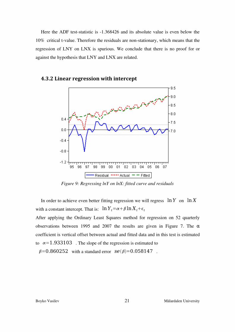
Here the ADF teststatistic is 1.368426 and its absolute value is even below the

10% critical tvalue. Therefore the residuals are nonstationary, which means that the

regression of LNY on LNX is spurious. We conclude that there is no proof for or

against the hypothesis that LNY and LNX are related.

4.3.2 Linear regression with intercept

In order to achieve even better fitting regression we will regress lnY on ln X

with a constant intercept. That is: lnY t= lnX tt

After applying the Ordinary Least Squares method for regression on 52 quarterly

observations between 1995 and 2007 the results are given in Figure 7. The α

coefficient is vertical offset between actual and fitted data and in this test is estimated

to =1.933103 . The slope of the regression is estimated to

=0.860252 with a standard error se=0.058147 .


Figure 9: Regressing lnY on lnX: fitted curve and residuals

The Rsquared statistic here is even higher, showing that 81% of the variance in

income level can be explained by changes in exports. The positive relationship

between the dependent and independent variables will be analysed once again by

hypothesis testing of H0 :=0 and H1 :0 at the 99% confidence level. The

teststatistic(14.79435) is larger than the critical tvalue even at 1% level of

significance t0.01,50=2.403272 , therefore we reject the null hypothesis

=0 at the 99% confidence level. This means that is positive and significanβ tly

different from zero. Despite the fact that we proved the statistical significance of the

regression coefficients, we should be careful about stating the existence of a

relationship between the regressor (LNX) and the regressand (LNY). Again the R2

value is greater than DurbinWatson (0.814038>0.789053), we have reasons to

suspect a spurious regression.

We see analogical results from the correlogram of the residuals. Here they start

considerably high and decline as we increase the number of lags. This gives us a

reason to suspect nonstationarity of the residuals. In order to confirm that we use

again the ADF unitroot test with an intercept and no trend:

t=t−11t−1...pt−put (10)

ADF tests the null hypothesis H0 :=0 is non-stationary versus the

alternative H1 :0 is stationary .


Figure 10: Regression results for lnY t= ln X tt

As we can see from the test results above the ADF test statistic is by absolute value

lower than the 5% critical value. Therefore we cannot reject the hypothesis of unit

root at the 5% significance level, and consequently the residuals of regressing LNY

on LNX with intercept are nonstationary. Therefore even this regression is spurious

and there is no evidence for the hypothesis that there is a relationship between LNY

and LNX.


Figure 11: ADF unitroot test on the residuals from lnY t= ln X tt

4.4 The co-integration method

I will perform cointegration tests on the time series for exports and income in

order to trace any longterm equilibrium relationship between the two variables. The

cointegration approach is considered superior to lestsquare regression and has been

widely used for analysing the relationship between nonstationary variables. Very

often the linear combination of two nonstationary time series of order I(1) is

spurious, which makes the results from the OLS regression irrelevant. Cointegration

theory, on the other hand, test whether the difference between two nonstationary

series produces a stationary sequence. If two variables are cointegrated they must

follow an equilibrium relationship in the longrun, even if they diverge considerably

from shortrun equilibrium.

The first step to cointegrating is to check if the variables to be analysed are non

stationary and of order of integration I(1), which are the necessary conditions for

cointegration analysis.

4.4.1 Augmented Dickey-Fuller unit-root test

The Augmented DickeyFuller(ADF) unitroot test will be used to determine

whether the series of logarithms of exports and income are nonstationary. The

econometric software package EViews6 will run the test and will automatically

calculate the tstatistics and critical values for hypothesis testing. The definition of an

I(1) series is that it is nonstationary, and its firstdifference is stationary. That is why

we can determine if the variables are I(1) series by testing its first difference for unit

root.

The ADF test with an intercept and no trend estimates the following equation:

Y t=Y t−11Y t−1...pY t−pt (11)


Here is the intercept constant, is the first lag of Y t ,and 1 ..p are

the coefficients of p lags of Y t . The econometric software uses the Schwartz

Info Criterion to determine a sufficient number of lags such that there is no

autocorrelation in the error terms t . The test for unitroot is based on the

coefficient of the lagged dependent variable Y t−1 .

We have to test the null hypothesis H0 :=0 Y is non-stationary against

the alternative H1 :0 Y is stationary . First let the test statistic be

tADF=

SE which has the tdistribution with n−2 degrees of freedom.

Here n is the number of observations, is the estimated firstlag coefficient from

equation (11), and SE is its standard error. For the LNX variable, we have the

following results:

From the figure above it can be concluded that tADF=0.510489 is outside the

rejection region tADFtn−20.01 , therefore we cannotot reject H0 and the series

LNX is nonstationary at the 1% significance level.

In order to check the order of integration of LNX, we apply the ADF on its first

difference:


Figure 12: ADF unitroot test on LNX (intercept, no trend)

In this case the test statistic is within the rejection region, therefore we reject H0

and conclude that D(LNX) is stationary.

As a result from the two unitroot tests above we can say that LNX is non

stationary of integration order I(1) and is suitable for cointegration.

For the logarithm of income LNY we have the following results from the ADF

unitroot test:

It is easy to see that tADF=0.094467 is outside the rejection region and the

hypothesis H0 of existence of unitroot cannot be rejected at the 1% significance level

Therefore the LNY variable is nonstationary.

Testing the first difference of the logarithm of income D(LNY) gives us:


Figure 13: ADF unitroot test for the first difference of LNX(intercept, no trend)

Figure 14: ADF unitroot test on LNY (intercept, no trend)

Here tADF=−6.561416 is within the rejection region and we reject H0 of the

existence of unitroot. Therefore the first difference of LNY is stationary and LNY is

of integration order I(1).

From the tests performed in this section we can conclude that the series for LNX

and LNY are nonstationary of order I(1) and are suitable for cointegration tests.


Figure 15: ADF unitroot test for the first difference of LNY(intercept, no trend)

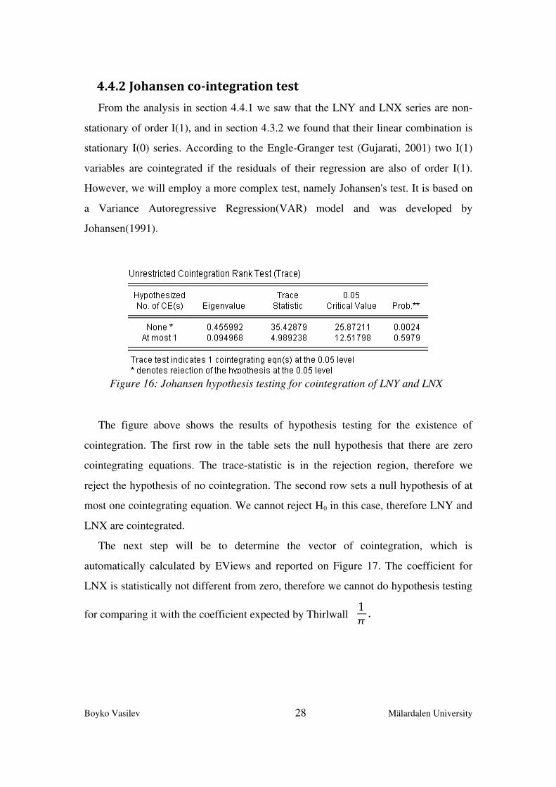
4.4.2 Johansen co-integration test

From the analysis in section 4.4.1 we saw that the LNY and LNX series are non

stationary of order I(1), and in section 4.3.2 we found that their linear combination is

stationary I(0) series. According to the EngleGranger test (Gujarati, 2001) two I(1)

variables are cointegrated if the residuals of their regression are also of order I(1).

However, we will employ a more complex test, namely Johansen's test. It is based on

a Variance Autoregressive Regression(VAR) model and was developed by

Johansen(1991).

The figure above shows the results of hypothesis testing for the existence of

cointegration. The first row in the table sets the null hypothesis that there are zero

cointegrating equations. The tracestatistic is in the rejection region, therefore we

reject the hypothesis of no cointegration. The second row sets a null hypothesis of at

most one cointegrating equation. We cannot reject H0 in this case, therefore LNY and

LNX are cointegrated.

The next step will be to determine the vector of cointegration, which is

automatically calculated by EViews and reported on Figure 17. The coefficient for

LNX is statistically not different from zero, therefore we cannot do hypothesis testing

for comparing it with the coefficient expected by Thirlwall 1

.


Figure 16: Johansen hypothesis testing for cointegration of LNY and LNX

4.5 Granger causality test

According to the original formulation of the law stated by Thirlwall(1979) GDP

growth is a function of the independent variable for growth of exports. In other words,

it is exports(X) that cause GDP(Y), and not the other way around. This view is typical

for Keynesian economists and can be expressed as XY. It is also possible that in

our case the causality runs in the opposite direction, namely Y X as neoclassical

economists claim.

In order to determine the direction of causality in the relationship I will use the

Granger causality test. This method looks at the matter to what extent current Y

values can be explained by its previous values, and whether adding lagged values of

X can improve this prediction. It is important to bear in mind that the statement “X

Grangercauses Y” does not mean that Y is the result of X. It just indicates that

past values of X bear some information about future values of Y .

According to Gujarati(2001) the Granger causality test assumes that the analysed

timeseries are stationary. However, X and Y proved to be nonstationary, and can

not be tested directly. Gujarati(2001, pp. 698) suggests that in such cases we can

analyse the first difference of the timeseries if it is stationary.

Here we have a twovariable causality test on DY and DX. This is favourable since

Granger causality test on more than two variables can return misleading results if


Figure 17: Cointegrating vector for LNY and LNX

there is auxiliary cointegration through a third variable. The Granger test is also

sensitive to the number of lags. Lags are the number of past time periods that could

help predict the target variable, and generally it is better to use more rather than few

lags. Here I chose 4 lags because I use quarterly data observations, and I believe that 1

year is the optimal time span within which some Granger causality can be observed.

The nullhypotheses for both directions are that there is no Grangercausality. The

pvalues in the last column indicate that we reject the null hypothesis that DY does not

Granger cause DX at less than 1% significance level. Therefore we can state that DY

Grangercauses DX, thus past values of DY can help predicting DX. In the second test

the null hypothesis of DX not causing DY cannot be rejected, which implies DX does

not Granger cause DY.

From the results above we can conclude that there is a unidirectional causality

DYDX , which contradicts Thirlwall's Keynesian model.


Figure 18: Granger causality test on DX and DY, using 4 lags

5. AnalysisIn this section I will summarise the findings from the empirical tests in the

previous section. It is very important to emphasise that the empirical tests in this study

employed Thirlwall's law in its generalised form. The assumption that the purchasing

powerparity holds even in fixed exchange rate regime has been made in order to

make empirical tests possible.

The Ordinary LeastSquares regression analysis in sections 4.3.12 with and

without intercepts showed statistically significant regression coefficients. However,

the R2 and DurbinWatson statistics raised suspicions about serial correlation of the

error terms and spurious regression. After investigating autocorrelations and

performing Augmented DickeyFuller tests on the error terms, those suspicions were

confirmed. There is spurious regression between the continuous rates of change in

exports and income(lnX and lnY respectively). Therefore the regression method can

not conclude whether there exists a relationship between these two variables, as

Thirlwall suggests. This is a common problem when analysing the linear combination

of nonstationary I(1) variables, and experience has shown that many timeseries in

macroeconomics behave exactly in this way. The failure to determine regression

coefficients does not allow us to perform hypothesis tests if it relates to the theoretical

value of 1

suggested by Thirlwall's law. That is why we had to resort to a more

sophisticated method.

The cointegration method was developed especially for detecting longrun

equilibrium relationships between nonstationary variables. It is based on the idea that

the errors from the linear combination of the related variables tend to disappear and

return to zero. The method can determine a long term equilibrium relationship even if

we have a small sample of data and the relationship does not hold in the shortrun. A

prerequisite for employing this method is that the involved timeseries should have a

unitroot (i.e. should be nonstationary). The Augmented DickeyFuller unitroot was

used for this purpose. After applying the test on the lnY and lnX variables they proved

to be nonstationary and therefore suitable for cointegration.


The Johansen(1991) cointegration test was performed in section 4.4.2. It proved

that the continuous rates of change in X and Y are cointegrated. The null hypothesis of

no cointegrating equations was rejected at less than 1% significance level, while the

hypothesis of (at most) 1 equations was not rejected. The test also produced

cointegration coefficient which unfortunately can not be analysed because it is

statistically not different from 0.

The third econometric test employed in this study is the Granger causality test.

Because it requires stationarity of the analysed variables, we used the first difference

of the I(1) variables X and Y and denoted it by DX and DY respectively. The results

was that DY Grangercauses DX at less than 1% significance level DYDX .

The nature of the test does not imply true causality, but states that movements in DY

precede and can to certain extent predict related movements in DX. The obtained

results contradict the specifications of the Thirlwall theoretic model, which postulates

demandled growth. Instead, in our empirical findings we see GDP causing exports,

which can be interpreted as supplyled growth.

Since exports follow GDP we cannot support the theoretical model of balanceof

payments constrained growth. We can also state that the Keynesian framework does

not match the empirical findings, and the classical approach of supplyled growth

might be more suitable for analysing this case.


6. Conclusions

The purpose of this study was to test empirically the validity of Thirlwall's law in

the case of Bulgaria. The incentive for this investigation was the increasing current

account deficit and steady economic growth of the Bulgarian economy. There have

been no other studies on this topic using Bulgarian data.

Thirlwall(1979) suggests that there is an optimal equilibrium rate of growth that

allows the economy to grow in a sustainable way. If the economy grows at this rate

and maintains a healthy balanceofpayments, it will be able to expand its production

capacity and will decrease its dependence on imports. It would also allow for a higher

equilibrium growth rates in the longrun.

The empirical investigation on the Bulgarian economy failed to provide exact

measure of the relationship between the analysed variables, and therefore Thirlwall's

model can not be proved onetoone in the Bulgarian economic history. Alternative

econometric techniques like cointegration and Granger causality proved the existence

of a longterm relationship between export growth and economic growth. However,

the latter test showed that the causality runs from income to exports(ΔY causes XΔ ),

which is the opposite to what the theoretical model suggests.

This leads us to the conclusion that there is a longrun relationship between exports

and domestic income, but it is exports that follow GDP. This allows us to reject the

Keynesian theory of exportled growth in the case of Bulgaria. This result may be due

to misspecifying the regression models in section 4 by using false assumptions. For

instance, the assumption of insignificance of the termsoftrade effect on the model.

We assumed this for the Bulgarian case for the sake of making empirical tests

possible, despite the fact that the Bulgarian economy operates under a Currency

Board Agreement with a hardpegged exchange rate. Such a exchange rate regime is

said to have negative effects on relative price levels, and therefore it might be the

reason for Thirlwall's model inconsistency in the case of the Bulgarian economy


Another possible explanation for the discouraging results may be the turbulent

economic conditions in the Bulgarian economy during the analysed time period. The

period(19952007) follows the transition from planned to marketing economy, and

some market mechanisms may still not be in place.


7. References

1. Atesoglu, Sonmez(1997), Balanceofpaymentsconstrained growth model and its implications for the United states, Journal of Post Keynesian Economics; Spring 1997; 19, 3; pp.327.

2. Dobrinsky, R.(2000), The transition crisis in Bulgaria, Cambridge Journal of Economics, 2000, 24, pp.581602.

3. Ferreira, A.,and Canuto, O.(2001), Thirlwall’s Law and Foreign Capital Service: the case of Brazil, Workshop “Macroeconomia Aberta Keynesiana Schumpeteriana uma Perspectiva Latino Americana”, Campinas, Brazil, June 2001.

4. Gujarati, N. Damodar(2002), Basic econometrics, 4th ed., McgrawHill, May 2002, ISBN 9780071123433.

5. Harrod, R.(1933), International Economics, Cambridge university Press, 1933

6. Johansen, S.(1991), Estimation and Hypothesis Testing of Cointegration Vectors in Gaussian Vector Autoregressive Models. Econometrica 59, 15511580.

7. McCombie, John S. L. (1997), On the empirics of balanceofpaymentsconstrained growth, Journal of Post Keynesian Economics, Spring 1997; 19, 3, pp. 345, ABI/INFORM Global.

8. McCombie, John S. L.,and Thirlwall, Anthony P. (1994): Economic Growth and the Balance of Payments Constraint, St Martin’s Press, New York.

9. MorenoBird, Juan Carlos(2003), Capital Flows, Interest Payments and the BalanceofPayments Constrained Growth Model: A Theoretical and Empirical Analysis, Metroeconomica 54 (23) , pp. 346–365 doi:10.1111/1467999X.00170 .

10. Romer, M. Paul(1986), Increasing Returns and LongRun Growth, The Journal of Political Economy, Vol.94, No.5 (Oct 1986), pp. 10021037.


11. Solow, M. Robert(1956), A Contribution to the Theory of Economic Growth, The Quarterly journal of Economics, The MIT Press, Vol.70, No.1(Feb 1956), pp.6594.

12. Thirlwall, A. P. (1980), Balanceofpayments theory and the United Kingdom experience, Palgrave Macmillan, ISBN: 0333243684.

13. Thirlwall, A. P.,and Hussain M. N. (1982): ‘The balance of payments constraint, capital flows and growth rates differences between developing countries’, Oxford Economic Papers, 34, pp. 498–509.

14. Thirlwall, A. P. (2006), Growth and development, with special reference to developing countries, Palgrave Macmillan, ISBN 1403996016.

15. Vasileva, E. (2002), Currency Board and the Bulgarian Experience, Agency for Economic Analysis and Forecasting. Bulgaria (2002)

16. Vasquez, Bismarck J. Arevilca and Charquero, Wiston Adrián Risso(2007). The balance of payments constrained growth model: empirical evidence for Bolivia, 19532002. Translated by Jeremy Jordan, Rev. humanid. cienc. soc. (St. Cruz Sierra) [online]. 2007, vol. 3.


Appendix


Year Quarter GDP (mil. €)

1995 Q1 1805.3 -72.6 861.6 882.1 383.01

Q2 2135 29.9 926.7 946.4 411.27

Q3 2783.5 180 1027.1 972.4 435.87

Q4 3238.5 -294.5 1021.7 1310.9 459.71

1996 Q1 2348 -115.7 891.6 994.1 402.17

Q2 2053 60.1 960.1 996.3 419.86

Q3 2092.3 166.4 929.9 951 412.72

Q4 1820.1 18.9 962.4 993 422.77

1997 Q1 1143.2 239.1 983.7 799.6 494.44 97.19%

Q2 2106.4 242.3 1071.4 1090.8 511.46 100.00%

Q3 3015 381.9 1130.9 1181.3 528.06 107.00%

Q4 2848.3 70 1070.3 1234.9 547.2 108.56%

1998 Q1 2422.8 -34.7 1006.3 1085 573.32 111.41%

Q2 2599.3 80.6 979.2 1099.5 571.35 106.47%

Q3 3227.3 112.2 893.3 1089.3 511.8 114.76%

Q4 3140.2 -186.6 868.1 1142.4 484.12 116.01%

1999 Q1 2519.3 -231.2 768.3 1056.4 475.94 114.89%

Q2 2692.9 -160.4 858 1244.4 491.28 109.88%

Q3 3443.1 30 1029.2 1344.6 563.71 116.24%

Q4 3508.6 -225.3 1078.2 1494.5 604.13 118.28%

2000 Q1 2880.6 -345.8 1114.6 1537.2 676.22 119.51%

Q2 3100.1 -90.8 1258.6 1641.1 712.19 117.56%

Q3 3857.6 84.4 1372.4 1759.5 767.22 120.86%

Q4 3869.2 -409.2 1507.5 2147.1 795.75 123.05%

2001 Q1 3282.8 -241.5 1398.5 1780.2 843.11 125.47%

Q2 3475.1 -167.3 1405.9 2085.6 895.12 121.64%

Q3 4284.6 -52.6 1498.8 2109.1 895.6 126.21%

Q4 4208.6 -393.7 1411.1 2153 834.19 126.76%

2002 Q1 3533.8 -185.5 1357 1779.4 866.51 130.64%

Q2 3866.8 -111.4 1470.8 2097.1 930.1 128.21%

Q3 4649 414.7 1683.7 2072.6 1011.75 129.06%

Q4 4574 -520.3 1551.4 2462.1 954.54 131.40%

Current Account (mil. €)

Exports (mil. €)

Imports (mil. €)

Exports to EU-25 (mil. €)

Real Effective Exchange Rate (CPI deflated) 1997Q2=100%

Sources: Bulgarian National Bank, National Statistical Institute


Year Quarter GDP (mil. €)

2003 Q1 3735.9 -300.3 1635.2 2083.6 1015.77 133.51%

Q2 4119.7 -419.9 1616.5 2457.3 1035.49 130.96%

Q3 4966.3 341 1752.5 2392.4 1108.54 132.57%

Q4 4946.3 -593.2 1664.1 2677.2 1053.94 139.96%

2004 Q1 4167.5 -462.5 1717.7 2411.9 1148.89 139.70%

Q2 4634 -402.3 1896.8 2919.5 1181.72 136.70%

Q3 5568.4 435 2183.8 2877.8 1335.71 138.96%

Q4 5503.6 -877.1 2186.6 3410.3 1304.62 141.72%

2005 Q1 4573 -579.4 2080.6 2961.7 1357.7 141.90%

Q2 5147.7 -596.5 2305.1 3630.1 1419.01 137.29%

Q3 6097.3 -243.6 2414.8 3795.6 1430.69 139.04%

Q4 6064.1 -1286.2 2665.9 4280.3 1494.38 141.52%

2006 Q1 5047.7 -1175.4 2672.5 3935.3 1684.35 146.44%

Q2 5969 -833.5 3053.7 4429.1 1824.19 145.81%

Q3 7056.6 -506.6 3197.7 4835.7 1945.42 144.25%

Q4 7165 -1974.9 3087.9 5279.2 1832.65 148.94%

2007 Q1 5771.3 -1574 2899.1 4697.3 1905.52 150.47%

Q2 6719.8 -1311.7 3305.9 5238.3 2019.25 148.87%

Q3 8049.5 -1020.1 3587.9 5656.9 2127.4 158.86%

Q4 8357.9 -2314.1 3680.6 6284.4 2113.11 161.88%

2008 Q1 -1670.8 167.33%

Current Account (mil. €)

Exports (mil. €)

Imports (mil. €)

Exports to EU-25 (mil. €)

Real Effective Exchange Rate (CPI deflated) 1997Q2=100%

Balance-of-payments constrained growth in the case of …139622/FULLTEXT01.pdf · Bachelor Thesis...

Documents

Transcript of Balance-of-payments constrained growth in the case of …139622/FULLTEXT01.pdf · Bachelor Thesis...