Bail Classification Profile Project - Harris County, Texas · In simplest terms, the Project has...

Bail Classification Profile Project

Harris County, Texas

Final Report

September 15, 1993

Steven Jay Cuvelier, Ph.D.

and

Dennis W. Potts, M.A.

Funded by a grant from the State Justice Institute

1 State

SJI Justice l Institute

1650 King Street, Suite 600 Alexandria, Virginia 2231 4

Bail Classification Profile Project

Harris County, Texas

H

Final Report

September 15,1993

Steven Jay Cuvelier, Ph.D. and

Dennis W. Potts, M.A.

This report was developed under Grant No. SJI-89-049 from the State Justice Institute. The points of view expressed are those of the authors, under the guidance of the grantee, and do not necessarily represent the official position or policies of the State Justice Institute.

-1 State

1-1 Institute S JI 1650 King Street, Suite 600 Alexandria, Virginia 2231 4

Justice

Table of Contents

The Authors ............................................................................................................................... v . . Acknowledgments ................................................................................................................... VII

Executive Summary of the Final Report ................................................................................. ix Scope of the Final Report Draft .................................................................................... xi What is the Bail Classification Profile Project? ............................................................... xi Project Goals ................................................................................................................ xii The Data ....................................................................................................................... xii Instrument Development and Testing .......................................................................... xii New Instrument Development and Testing ................................................................... xiv The Eight-Item Model ................................................................................................... xv

..................................................................................... Examining Pretrial Misconduct xvi ... Disparate Impact ........................................................................................................ x v ~ ~

Summary and Conclusions ..................................................................................... xix

..................................................................................................... Full Text of the Final Report 1 . ....................................................................................................... Section One Introduction 3

Scope of the Report ........................................................................................................ 3 ................................................................ What is the Bail Classification Profile Project? 3

Bail and Pretrial Release in Hanis County ....................................................................... 4

Pretrial Services and Alberti ............................................................................................ 6 .................................................................................................. PTSA Risk Assessment 7

PTSA Today ................................................................................................................... 8 The County Justice Environment Today ........................................................................ 10

Section Two . The Role of Classification and Prediction in Justice Decisionmaking ........ 13 Introduction ................................................................................................................... 13 Classification: Epistemological Issues ..................................................................... 13 . Prediction: Statistical Issues .......................................................................................... 18 Criterion. Base Rate. and Error ..................................................................................... 24 Conclusion ................................................................................................................. 25

Section Three . Methodology ................................................................................................. 27 Introduction ................................................................................................................... 27 Methodological Overview ............................................................................................. -28 The Study's Goals ......................................................................................................... 28

...................................................................................... Methodological Underpinnings 29 Instrument Testing Concepts and Procedures ............................................................... 32 Instrument Development and Testing Methods for this Study ........................................ 39

................................................................................................................ The Variables 39 Variable Transformation ................................................................................................ 40

Instrument Development .............................................................................................. -41 Validation Procedures ................................................................................................... 42

............................................... Testing Disparate Impact by RaceIEthnicity and Gender 44

. ............................................................ . Section Four Descriptive Data for the 1990 Sample 47 Introduction ................................................................................................................... 47 Data Quality .................................................................................................................. 47 Descriptives ................................................................................................................. 48 Conclusion ................................................................................................................ 52

............................................................ . Section Five Instrument Development and Testing 55 The Findings ................................................................................................................. 55

................................................................................................. The Former Instrument 55 .......................................................................................... The Reweighted Instrument 57

New Instrument Development .......................... :. ....................................................... 62 ......................................................................................... Testing the New Instruments 70

Conciusions .................................................................................................................. 76

Section Six . Implementation .................................................................................................. 77 Introduction ................................................................................................................. 77 How and When ............................................................................................................. 77 Reaction to the New Instrument .................................................................................... 78 Conclusion .................................................................................................................... 80

Section Seven . Projecting Outcomes with the 1991 Data .................................................... 83 Introduction ................................................................................................................... 83

............................................................................................................. Data Collection 83 Descriptives .................................................................................................................. 83

........................................................................................................................ Findings 85

Section Eight . Instrument Validation on Actual Experience from 1993 .............................. 91 Introduction ................................................................................................................... 91 *

The Data ....................................................................................................................... 91 ..................................................................................................... Data Quality 91 .................................................................................................... Descriptives -91

Comparison to the 1990 Sample ...................................................................... 95 Examining the Instrument's Performance ...................................................................... 97

Differentiating Failure Rates from the Base Rate and Classification Levels .............................................................................................................. 97 Consistency Over Time .................................................................................. 100

Reconstructing the Instrument ..................................................................................... 103 .......................................................................... Constructing the New Scores 103

The Results .................................................................................................... 105 Conclusions ................................................................................................................ 106

I

Section Nine . The Impact of Classification on Minorities and Females ........................... 109 Introduction ................................................................................................................. 109 What Can be Leamed from Disparate Impact Studies? ............................................. 111 Examining the Classification Instrument for Disparate Impact ..................................... 111 .

................................................................................................................ Conclusions 123

............................. Section Ten . Using Classification Information for Strategic Planning 127 ................................................................................................................ Introduction 1 27

................................................. The Disposition of Non Released Pretrial Defendants 127 ....................................................... Impact of Release Policies on the Jail Population 129

Conclusions ................................................................................................................ 131

Section Eleven . Summary and Conclusions ...................................................................... 133 Introduction ................................................................................................................. 133 Findings ............................................................ ......................................................... 133

.................................................................................... Comparing Alternative Models 134 ........................................................................................................... Implementation 136

.................................................................................................................... Validation 136 Disparate Impact ......................................................................................................... 138 Conclusions ............................................................................................................ 139

Bibliography .......................................................................................................................... 141

................................... Appendix A . Variables Extracted from the JlMS Data for Analysis 1 4

............................... Appendix B . Calculating the Mean Cost Rating and Rated Accuracy 149

iii

THE AUTHORS

- STEVEN JAY CUVELIER, Ph.D. is an Assistant Professor of Criminal Justice at the George J. Beto Criminal Justice Center of Sam Houston State University in Huntsville, Texas, where he also serves as the Director of Information Resources. A Senior Research Associate with the National Council on Crime and Delinquency, Cuvelier is a former analyst with the Research Bureau of the Ohio Department of Corrections and remains active in the area of prison population projection. Dr. Cuvelier has published articles primarily dealing with computer simulation in criminal justice systems and is the author of Prophet, a computer program used in the development of policy simulations for prison systems.

DENNIS W. POTTS, M.A. is a doctoral student at the George J. Beto Criminal Justice Center of Sam Houston State University in Huntsville, Texas, and he is employed as a supervisor in the Court Services Division of the Harris County Pretrial Services Agency in Houston, Texas. Mr. Potts has previously worked in both municipal and state-level law enforcement, as a Parole Caseworker with the former Texas Board of Pardons and Paroles, and as an Adult Probation and Parole Agent with the Louisiana Department of Public Safety and Corrections. He has co- authored articles dealing with prosecutorial liability, role perceptions of probation officers, and criminal justice ethics.

0

This report was developed under Grant No. SJI-89-049 from the State Justice Institute. The points of view expressed are those of the authors, under the guidance of the grantee, and do not necessarily represent the official position or policies of the State Justice Institute.

I Institute

1650 King Street, Suite 600 Alexandria, Virginia 22314

ACKNOWLEDGMENTS

The authors wish to acknowledge the participation and assistance of the following: -

Hams County Commissioners' Court Honorable Jon Lindsay, County Judge

Richard L. Raycraft, County Budget Officer

Hams County District Courts Trying Criminal Cases Honorable Miron Love, Administrative Judge

Jack Thompson, Administrator

Hams County Criminal Cpurts at Law Bob Wessels, Administrator

Hams County Pretrial Services Agency Charles Noble, Director

Carol Oeller, Assistant Director

Stevens H. Clarke, L1.B. University of North Carolina at Chapel Hill

Chapel Hill, North Carolina

Joycelyn Pollock-Byme, Ph.D., J.D. University of Houston - Downtown Campus

Houston, Texas

vii

There is nothing so admirable about the status quo and its conventional wisdom, in decision making or anything else, that we need either to exalt or to perpetuate it.

\

viii

Bail Classification Profile Project Harris County, Texas

Executive Summary of

Final Report

Scope of the Final Report Draft

This Final Report, prepared as part of the Bail Classification Profile Project, is the end product of the Bail ~laki f icat ion Profile Project conductedfor the Hams County Pretrial Services - Agency (PTSA), located in Houston, Texas. This report focuses on the basic issues of prediction classification, how a new point scale was designed for Hams County, and how that scale performed after implementation.

What is the Bail Classification Profile Project?

The central issue underlying the Project was whether the existing predictive tool or an empirically-derived instrument would offer the consumer courts greater predictive accuracy in making pretrial release decisions. To that end, the Project was conceived solely as a way to develop and evaluate an empirically-validated predictive tool through the combined use of paper files and automated data.

Our approach to these questions was rooted in the knowledge that pretrial misconduct is a relatively infrequent event and that large numbers of cases would be necessary to achieve stable results; it seemed impractical to follow more traditional methods of data collection and analysis. Instead of utilizing archived, hard-copy manual applications, we sought to use data from the defendant interviews that have been maintained in the county's information management system since late 1989. Through proper manipulation, we believed that pretrial data could be processed much more efficiently, and that larger numbers of cases could be examined across a wider range of variables than would be possible by hand-coding. Furthermore, the effective use of automated data was expected to provide a track upon which future evaluations could be built, requiring less time and resources than would traditional evaluation methods.

In simplest terms, the Project has been an effort to use existing, county-maintained, automated data to develop a framework for policy decisions pertaining to the pretrial release of Hams County criminal defendants. Optimally, such a framework should: (a) permit decisionmakers to estimate the degree of risk involved in the release of a defendant, with particular attention to the risk that the defendant would not appear in court as scheduled (failure to appear, or FTA) or that the defendant will engage in further criminal activity; (b) enable policymakers to balance the competing concerns of public safety, public opinion, court mandates, cost-effective use of system resources, and justice; and (c) establish and maintain an ongoing, automated evaluation process to continue the classification instrument as a quality, low-cost decision tool responsive to the ever-changing context of criminal justice.

From the outset, it was important to focus on the notion of the development and implementation of a decision framework; this instrument was not intended to be an incursion into judicial responsibilities, but an aid to judicial officers in making pretrial release decisions. The intended product was a decision support tool that would distill for the court concise information about extralegal factors which appeared to have substantive or statistical relevance to the decisionma king process.

m

I

Project Goals

The fundamental, immediate goal of the Project was to assess the performance of the present bail classification instrument used by PTSA and to develop an alternative instrument that -

could be implemented by the Agency should it prove sufficiently more effective in classifying defendants on their likelihood of pretrial misconduct.

As a long-term goal, the Project sought to establish ongoing, automated evaluation tools in Hams County that would allow cost-effective monitoring and "fine tuningw of the classification instrument, thus keeping it current with the dynamic decisionmaking environment of criminal justice. By detecting patterns as they emerge, a continually-updated instrument could be used to identify characteristics and policies that appear to have positive or negative effects on pretrial behavior. Also, by receiving timely information on changes in the defendant population or the system behavior from evaluations of this sort, policymakers could determine what adjustments might be appropriate and/or necessary to maintain consistent pretrial release policies. Such adjustments should not have to wait any number of years-particularly if the agency can access the tools and knowledge required for immediate replication and correction.

The Data

The data for the construction phase of this study were drawn from 1990. For that year, in which 53,550 defendant interviews were conducted, we were able to access 31,418 defendant interviews (58.2 percent) through the Justice Information Management System (JIMS) for descriptive analysis. Ultimately, 6,796 of these interviews were matched to corresponding case data obtained from JIMS and used for instrument construction.

For comparison, data were also drawn from 1991, which gave us access to 37,701 defendant mlewiewf. -This yielded 4&589-cases~hich were-maEhed-to gsedata, and these - - -

data were used for confirmatory purposes not specifically required for this study and for assessing disparate impact based on racdethnicity or gender.

Finally, data were drawn from the first quarter of 1993 (January to March) for validation of the instrument constructed on the 1990 data. These data provided access to 10,283 defendant interviews, or 74.5 percent of the 13,794 interviews that were reported by the Agency during that period. Of these, 4,710 received some form of pretrial release, and those cases were used to validate the predictive instrument that was constructed on 1990 data. As well, these data were used in the assessment of disparate impact.

Instrument Development and Testing

The Former Model

The former instrument-based upon the Vera point scale developed in New York in the 1960s--combined six items reflecting community ties and failure to appear history with the defendant's prior criminal record to produce a risk score. The defendant's response to each of the items on the instrument was scored according to the point scale shown in Figure 1. The point total could run from a high of 7 points to a low that was determined by the prior criminal

xii

history of the defendant. In the analysis of 1990 data, the low score was -22. Applications with scores of 4 or higher were considered eligible for presentation to the judges for personal bond release consideration. From that, we inferred that defendants meeting those criteria were thought to be better risks than those who fell below that cutoff point. -

Defendants who achieved any form of pretrial release were traced to final case disposition. Any who were rearrested for offenses committed while awaiting trial, or any for whom warrants were issued for failure to appear, were identified as failures; the others for whom no official action was recorded were considered successes. All released inmates were grouped according to their classification scores, and the proportion of successes to failures were calculated. Figure 2 shows the rate and distribution of failures by classification score.

Figure 1. Former Bail Classification Items and Scoring

I Resides in county +1 if defendant lives in Harris County. I

Telephone in home +1 if true.

Whom defendant lives with +1 if def. lives with parents, spouse andlor children

Length of residence + I if 1 year ar more

Employment + I if fulVpart time employed, disabled, or homemaker

Prior FTA +1 if defendant had no prior failures to appear

Prior convictions -1 for each prior felony and misdemeanor, with the first

I misdemtem waived.

11 I + I if no priors or 1 prior misdemeanor

Figure 2. Distribution of Failures by the Fonner

Instrument Classification Score - -

Score Number of Number of Successes Failures

1 37 29

098 130

123 3 1

1 79 36

280 52

559 81

885 131

1,378 1 42

1,602 123

Total Failure Rate

! Total 6.041 755 6.796 0.1 11

Lower Limit

0.086

0.095

0.104

0.091

0.097

0.087

0.097

0.071

0.053

Upper Limit

0 . m

0.1 58

0.298

0.244

0.21 6

0.166

0.1 60

0.1 I 6

0.090

Percent of Population

2.44%

15.13%

2.27%

3.1 6%

4.89%

9.42%

14.95%

22.37%

25.38%

The former instrument was scaled so that lower scores denoted higher risks, as seen in Figure 2, where the failure rates generally trend from high to low across defendant classes. The first category consists of all negative scores; combining them was necessary since there were so few cases in any of those categories.

xiii

With the exception of the first two categories, Figure 2 shows a general downward trend as the classification scores increased. The second category (defendants scoring 0) appeared to be more related to categories 6 and 7 (scores of 4 or 5) than it was to categories 1 and 3 (scores of -1 or 1). Only the lowest risk group (scores of 7) fell clearly below the overall average. All other groups included the average as part of their respective confidence intervals. This suggests that the current instrument did not differentiate cases on the basis of risk very well.

Figure 3 shows the mean cost rating (MCR) for the former model. With a rating of 0.1635 (on a scale of 0 to I), the model was confirmed to have low predictive capability. Even that may be overstated, in that the classification efficiency rating method used was insensitive to order. If it is assumed that risk is associated linearly with a score (i.e., the lower the score, the greater the risk), the instrument actually performed below indicated levels.

Figure 3. Classification Efficiency of the Former Model

Score 7

6

5 4

3

2

1

0

< 0

F r q Succ 137

898

1 23 1 79

260

559 885

1,378

1,602

F r q Fail 29

130

3 1

36 52

8 1

131

1 42

1 23

Base Rate 0.1 11 1

- - - The primary pfobtem w i t h t k i R W m m t was tkatShere-was no balance betweenfacto~ that were more influential and those that were less so; all factors were weighted equally in arriving at a total score. Therefore, a defendant with two prior felonies and a telephone would have been classified the same as a defendant with one prior and no telephone.

0

New Instrument Development and Testing

Instrument development refers to the process of evaluating available data to determine which combination will render the best prediction of pretrial misconduct. The process of '

developing a stable and predictive model was not a simple, one-step operation; variables were examined in a variety of combinations to determine which ones worked together to bring about the desired ends. We developed three new models that were based upon the best of 40 predictors developed in this study. The question remained as to how well they classified defendants on the basis of risk. Their testing involved applying the weights developed in the previous section as an interviewer might have applied them as defendants were processed through the pretrial process. Once the scores were assigned, the cases were grouped according to their classification scores and successes were separated from failures. Of the three

xiv

I

alternative models offered (a five-, a nine-, and an eight-item model), the Agency elected to implement the eight-item model.

The Eight-Item Model -

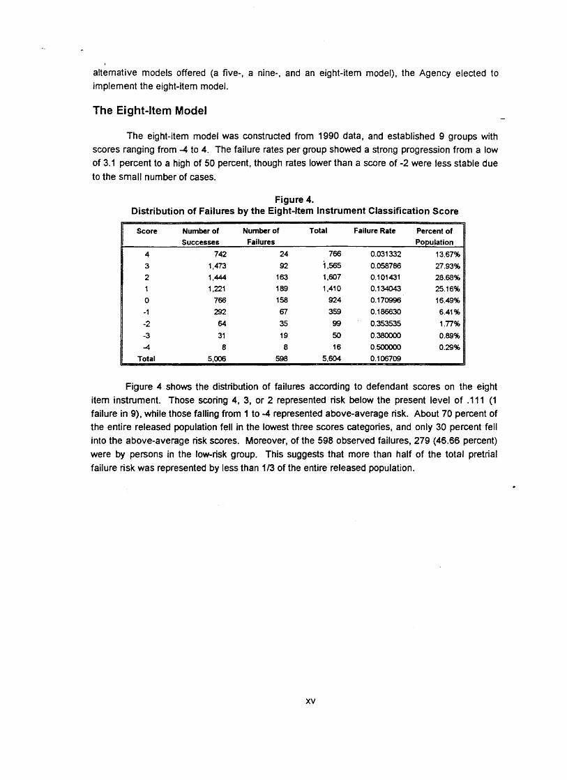
The eight-item model was constructed from 1990 data, and established 9 groups with scores ranging from -4 to 4. The failure rates per group showed a strong progression from a low of 3.1 percent to a high of 50 percent, though rates lower than a score of -2 were less stable due to the small number of cases.

Figure 4. Distribution of Failures by the Eight-Item Instrument Classification Score

Score Number of Number of Total Failure Rate Percent of

Successes Failures Population

4 742 24 766 0.031 332 13.67%

3 1,473 92 1,565 0.058786 27.93% 2 1,444 1 63 1,607 0.1 01 431 28.68%

1 1,221 189 1,410 0.1 34043 25.16%

0 766 1 58 924 0.170996 16.49%

-1 292 67 359 0.1 86630 6.41 %

-2 64 35 99 0.35~35 i .n% 3 31 19 50 0.380000 0.89%

4 8 8 16 0.500000 0.29%

Total 598 5,604 0.1 06709 *

Figure 4 shows the distribution of failures according to defendant scores on the eight item instrument. Those scoring 4, 3, or 2 represented risk below the present level of .I11 (1 failure in 9), while those falling from 1 to -4 represented above-average risk. About 70 percent of the entire released population fell in the lowest three scores categories, and only 30 percent fell into the above-average risk scores. Moreover, of the 598 observed failures, 279 (46.66 percent) were by persons in the low-risk group. This suggests that more than half of the total pretrial failure risk was represented by less than 113 of the entire released population.

Figure 5. Classification Efficiency of the Eight-Item Instrument

Score F W Prop P(Cum) Freq Succ Freq Fail P(Success)

-3 50 0.0074 0.0097 31 19 0.0051

Total 6,796 6,041 755 Base Rate 0.1 067

The mean cost rating of the eight-item model, shown in Figure 5, doubled that of the former model (.3251 compared to .I 635 for the former model).

Examining Pretrial Misconduct

Using 1993 data, each defendant was assigned a score using the classification instrument's criteria, and the interview data were linked to case data, as was done with the 1990 data. Figure 6 shows the rate and distribution of failures by classification score.

Only 58 (1.23 percent) of the 4,710 released defendants scored less than -1 on the instrument, and those defendants were grouped into the "less than -1" category ( 4 ) . All categories showed a monotonic (stairstep) decrease in their misconduct rate, ranging from 27.59 percent for classification scores less than -1, to 3.76 percent for level 4. Further, the proportion of the released population represented by those levels grew from a minimum of 58 cases for scores less than -1, to a maximum of 1,203 cases with classification scores of 3. Those groups posing the greatest level of risk tended to have few cases. Combining cases with scores of 1 or less revealed that 53.10 percent (266f501) of the misconduct cases could be attributed to classes representing 33.72 percent (1588f4710) of the released defendant population (half of the

*

observed misconduct was attributable to one-third of the sample defendants).

xvi

Figure 6. Rate and Distribution of Failures by Classification Score

The central question to be addressed was whether the classification instrument provided a valid assessment of risk; that question must be anskered in two ways. First, the instrument

Classification Score

should have produced different failure rates for each classification level and the rates should have changed monotonically between levels. Second, the failure rates should have been somewhat consistent over time. The first set of conditions are required since the purpose of classification is to group cases into homogeneous categories, and the existence of different categories implies different risk levels. It is further required that the risk levels for each successive category change monotonically, since typical usage involves setting a break point (i.e., consideration of cases with scores greater than 0). This necessitates that categories above the break point consistently represent less risk than those categories falling below. The second condition stipulates that the failure rates should be somewhat consistent over time, realizing that the subjective nature of decisionmaking can alter conditions, and realizing that random variation inherent to criminal justice activity will produce fluctuations in observed behavior.

Addressing the first condition, we confirmed through calculations that the differences between groups 4 and 3, 3 and 2,2 and 1, and 0 and -1 were statistically significant at p > .01. Differences between groups 1 and 0 and between groups -1 and <-I were not significant. While we would like to have found clear distinctions between each of the groups, the above differences did not fall outside the range of expected variation.

O

The second requirement of the instrument is that of consistency over time. Comparing the 1993 experience with the predictions made on the basis of 1990 data showed that the 1993 misconduct base rate differed by about one-half of one percent, compared to the base rate for 1990. This suggested that little had changed in the overall performance of persons released during the pretrial stage. Comparing across classification scores, the two most notable changes occurred in the highest-risk categories. The misconduct rate for scores less than -1 dropped from 37.58 percent to 27.59 percent, while the misconduct rate for category -1 increased from 18.66 percent to 25.00 percent between the predicted and actual experience. These differences may be due to random fluctuation as the total number of cases in those two groups were very small, representing less than 8 percent of the total sample in the 1990 data and less than 5 percent in the 1993 data.

When comparing the predicted failure rates from the 1990 sample to the actual rates observed in the 1993 data (Figure 7), we noted that the percent of the population falling into

I - Number of Successes

xvii

Number of Failures

Total Cases

- -

Misconduct Rate

- --


I

each of the categories formed a pattern of change. The changes in the proportion of defendants in each classification category between the 1990 and 1993 data sets (Figure 7, "Percent of Population" column) were statistically significant, with the exception of classification level 2. The t values for each level from <-I to 4, respectively, were: -2.64053, -6.49696, -1 1.6924, -2.1 6388,- 0.6731 07, 5.3361 8, and 10.23608.~ The high-risk categories (less than 1) experienced reductions in the proportion of releases in 1993 relative to 1990. By contrast, the lower-risk categories (3 and 4) showed substantial increases in their proportions.

Figure 7. Comparison of Predicted and Actual Failures by Classification Score

Predicted from 1990 Data Actual 1993 Experience I Difference I I 11 Classification I Misconduct Percent of I Misconduct Percent of I Misconduct Percent of 11

Disparate Impact

I,

With any policy decision there are both intended and unintended consequences. When policy decisions are applied to the classification of defendants there may be a very fine line

Score

C-1

-1

0

1

2

between what is intended and unintended. The goal of pretrial classification is to differentiate between groups of defendants with distinctly different failure rates. To the extent that the instrument accomplishes this, we are compelled to conclude that the eight-item model is valid.

Rate Population

When groups of defendants are found in disproportionate numbers in any category, however,

37.58%

18.66%

17.1 0%

13.40%

10.1 4%

questions concerning the legitimacy of the classification process are raised. What often gets lost

Rate Population

2.43%

5.28%

13.60%

20.75%

23.65%

in these discussions is the difference between information describing what the jurisdiction's

27.59%

25.00%

16.1 7%

14.49%

10.56%

Rate Population

experience has been and judgments defining what the jurisdiction's experience ought to have -

1.23%

3.65%

12.87%

15.97%

22.1 2%

-9.99%

6.34%

-0.93%

1.09%

0.42%

been.

-1 20%

-1 53%

-0.73%

-4.78%

-1 5 3 %

While the classification instrument itself was shown to work reliably, we found that there were some discrepancies in the way in which some defendant groups were classified. The discrepancies, while statistically significant, did not represent excessive differences. When the classification scores were grouped according to broad risk levels (4,3, and 2 representing low risk, 1 and 0 representing medium risk, and -1 and <-1 representing high risk), the differences between most groups dropped out. Only females and males remained split, with females in group 2 representing low risk, but males in that group representing more of a medium risk. Even in group-by-group comparisons, differences were found to be significant, but not necessarily substantial.

A value of k1.96 or more is required to establish a significant relationship.

xviii

In the context of this research, when groups are not evenly distributed across levels of risk, any attempt at treating the groups equally can result in bias (the unequal treatment of equivalents). This is most likely to occur when key variables are left out of the analysis. It is difficult to imagine any variable that is not associated disproportionately with race/ethnicity or- gender. Offense type, social, and economic variables all posses a degree of disproportionality with respect to the "prohibited" variables. This makes them vulnerable to statistical bias.

The type of bias more likely to be sought out is related to the fair treatment of defendants by the system. "Fairness" and other terms related to justice issues are rooted in our values systems and philosophy. Much of what goes into values falls outside of the JlMS system and our ability to capture and analyze data. We can report the Hanis County experience as succinctly as possible in the form of a classification instrument, but we must relegate the concerns for justice to the political sphere where such issues can more effectively be addressed.

These constraints notwithstanding, further analysis using "prohibited" variables demonstrated that the current classification model is identical to one in which the impact of racelethnicity and gender has been taken into account. This suggests that the present set of predictors are functioning without direct bias against racelethnicity or gender. Deviations in failure rates between groups at certain risk levels may be due to random variation or due to the crudity of the additive points scale approach to classification; that is, by reducing coefficients to integer values to aid score computation, we may be blunting the instrument's ability to make fine distinctions. If either of these possibilities are responsible for the observed differences, they should not remain the same over time. Subsequent analyses should show new patterns (though not radically different) between defendant groups.

Summary and Conclusions

In the broadest terms, this project attempts to provide Hanis County with a decision support framework for criminal justice. We use the term "framework" in recognition that this study offers a change in the way we think of data and the uses to which it may be put. This framework: (1) enables decisionmakers to estimate the degree of risk involved in the release of a defendant, (2) enables policymakers to balance the competing concerns of public safety, public opinion, court mandates, cost effective administration of resources, and justice; and (3) establish and maintain an ongoing, automated process to assure that a quality, low-cost decision support tool is maintained.

We developed a bail classification instrument using 8 predictors of 40 that were developed from data available through the JlMS data for the 1990 defendant population. We found the instrument to be substantially more predictive of outcome than the original instrument used in Hams County for more than decade.

Tests for disparate impact on defendants of different raciallethnic backgrounds or sex show some differences, but these fall within limits one may expect from random variation. Statistically removing the influences of racelethnicity and sex from the classification instrument caused no change in the way the instrument predicts risk.

We may therefore conclude that the instrument is performing its intended function well and should be applied widely as a credible information source in making bail decisions.

xix

Full Text of the Final Report

Section One Introduction

Scope of the Report

This document is a product of the Bail Classification Profile Project (hereafter "Project"), prepared for the Hams County Pretrial Services Agency, located in Houston, Texas. This report focuses on the basic issues of prediction classification, how a new point scale was designed for Hanis County, and how that scale performed after implementation.

What is the Bail Classification Profile Project?

The impetus for the Project was manifold. The Hams County Pretrial Services Agency (PTSA) was providing release eligibility information to Hamis County judges using an instrument that was based on the original Vera point scale used in the Manhattan Bail Project (see Ares, Rankin, and Sturz, 1963). For some time, PTSA officials had expressed concern that the instrument had never been validated, that its worth as a predictive tool had not been established, and that they knew of no attempts to examine its applicability across temporal or regional differences. Officials also expressed concern about a serious jail overcrowding problem which, while primarily due to a backlog of inmates awaiting transfer to the state prison system, was exacerbated by a substantial pretrial population and the under-utilization of pretrial release options.

The central issue underlying the Project was whether the existing predictive tool or an empirically-derived instrument would offer the presiding judges greater predictive accuracy in making pretrial release decisions. To that end, the Project was conceived solely as a way to develop and evaluate an empirically-validated predictive tool through the combined use of paper files and automated data.

Our approach to these questions was rooted in the knowledge that pretrial misconduct is a relatively infrequent event and that large numbers of cases would be necessary to achieve stable results; it seemed impractical to follow more traditional methods of data collection and analysis. Instead of utilizing archived, hard-copy manual applications which would require hand- coding, we sought to use data from the defendant interviews that have been maintained in the county's information management system since late 1989. Through proper manipulation, we believed that pretrial data could be processed much more efficiently, and that larger numbers of cases could be examined across a wider range of variables than would be possible by hand- coding, given the Project's time and resource constraints. Furthermore, the effective use of automated data was expected to provide a track upon which future evaluations could be built, requiring less time and resources than would traditional evaluation methods.

In simplest terms, the Project has been an effort to use existing, county-maintained, automated data to develop a framework for policy decisions pertaining to the pretrial release of Hams County criminal defendants2 Optimally, such a framework was expected to:

The term defendant was favored over the term errestee because no person arrested in Hams County is eligible for release

on bail unless he or she has been officially charged with a criminal offense.

(a) permit decisionmakers to estimate the degree of risk involved in the release of a defendant, with particular attention to the risk that the defendant would not appear in court as scheduled (failure to appear, or FTA) or that the

- defendant would engage in further criminal activity;

(b) enable policymakers to balance the competing concerns of public safety, public opinion, court mandates, cost-effective use of system resources, and justice; and

(c) establish and maintain an ongoing, automated process to assure a quality, low-cost decision tool responsive to the ever-changing landscape of criminal justice.

From the outset, it was important to focus on the notion of the development and implementation of a framework; this was not to be an incursion into judicial responsibilities, but an aid to judicial officers in making pretrial release decisions. The intended product was a decision support tool that would distill for the court concise information about extralegal factors which appeared to have substantive or statistical relevance to the decisionmaking process.

Bail and Pretrial Release in Hams County

The practice of having an accused person provide surety for appearance before a tribunal is found in the works of plato3 and, in its more familiar form, has existed since the 7th Century, A.D. in England. For more than a millennium, bail has served the ends of the court by assuring that the defendant would appear to answer charges. In Texas, this purpose has been codified to permit surety in the form of both bail bonds and personal bonds.4

Under Texas law, the term bail bonds refers to both cash bonds and surety bonds. A cash bond is a form of surety submitted by the defendant in the form of valid United States currency, which is refundable to the person who provided the bail upon satisfactory compliance with the conditions of release by the defendant, and upon order of the court.5 Alternatively, bail may also be posted by one or more persons on behalf of the defendant in a form referred to as a surety bond. Typically, this type of bail is posted by a commercial bail bondsman with whom the defendant-or his or her agent-has executed an agreement. These agreements generally take the form of a nonrefundable fee in conjunction with a written agreement to indemnify the bondsman in the event of the defendant's nonappearance. Under either circumstance, the defendant or surety executes a written agreement to pay the principal amount--plus expenses-if the defendant violates the terms of his or her bond.

By contrast, the personal bond is a discretionary instrument available to judicial officers which permits the release of a defendant in return for his or her promise to appear in court. If approved for release in this manner, a defendant is required to sign a form giving assurance of

See Samaha (1 991 : 298).

Article 17.01, Texas Code of Criminal Procedure.

Article 17.02, Texas Code of Criminal Procedure.

I

his or her appearance at the appointed date and time, and promising to pay the full amount of the bail-plus expenses-if he or she fails in that obligation. These personal bonds may be handled through the approving court, but Texas law also provides for the establishment of personal bond offices to gather and review information to be presented to the appropriate court.6 - While in many respects the personal bond-as a form of unsupervised release-is equivalent to release on recognizance, a fee may be required of defendants who are released on the recommendation of the personal bond off im7 Fees, which are minimal compared to those of commercial bail bondsmen, are by law to be used solely to defray the expenses of the personal bond office.

Each of these types of bail serves the same function by allowing a defendant to be released from jail, but whether a defendant is able to financially afford release or must wait for release on a personal bond presents both costs and benefits. Harris County utilizes a bond schedule to speed cash and surety bail releases from jail. The schedule sets forth a fixed bail amount based on the offense charged and the defendant's number of prior convictions, and the scheduled amount applies as soon as the defendant is formally charged with an offense. This arrangement permits some defendants to post bail at outlying facilities and to avoid transfer to the county jail, thus removing them from the process at an early stage and inconveniencing them for a shorter period than those defendants who cannot arrange immediate financial release. Defendants who are charged with a misdemeanor and cannot make bail are transferred to the county jail, where they have an opportunity for bail review and for probable cause determination before a magistrate at hearings scheduled throughout the night.8 Defendants who are charged with a felony and who are otherwise unable to post bail are held until the following morning, when they are taken before a district court judge for bail review and a probable cause hearing.9

On the one hand, the bond schedule provides certain benefits by lessening the number of prisoners transferred to the county jail, thus allowing some defendants to return to their normal activities, and by easing the strain on jail facilities and crowded court dockets. On the other hand, defendants who make bail prior to their appearance before a judge return to the community without judicial review of the circumstances of the offense and with little or no pretrial supervision or assistance. Further, because the amounts on the schedule are arbitrarily set, a situation exists in which defendants who may present a significant risk to the community can be set free simply because they can financially afford their release while defendants who present little or no risk can-for lack of money-be detained.1°

Article 17.42(1), Texas Code of Criminal Procedure.

Article 17.42(4), Texas Code of Criminal Procedure. The court may assess the greater of twenty dollars or three percent

of the bond amount, or the fee may be decreased or waived for cause.

As a part of bail review, the magistrate also applies guidelines set forth by the misdemeanor judges to make decisions

regarding release on personal bond.

This process is somewhat altered on weekends, when a number of judges have indicated they do not want personal bond

applications for defendants assigned to their courts to be presented to the weekend duty judge. Therefore, some

defendants who are arrested on Friday do not have an opportunity for personal bond release until the following Monday.

The use of a bail schedule has been questioned because Texas law requires that the determination of bail amounts must take into account the circumstances of the offense and the abildy of the defendant to make bail, and the use of a standardized schedule which sets bail amounts without consideration of these points is at variance with the controlling

statute (see Art. 17.1 5 Texas Code of Criminal Procedure for factors to be considered in setting bail, and Texas Attomey

Pretrial Services and Alberti

In Houston, a small number of personal bonds are handled solely by the approving court, but most are effected with the assistance of the Hams County Pretrial Services Agency (PTSA). -

This agency began its existence in the late 1960's as a by-produd of a Ford Foundation grant to the Criminal Division of the Houston Legal Foundation. At that time, the Pretrial Release Program (as it was then named) focused only on determining eligibility for indigent defendants who were charged with a limited range of offenses. The initial funding source lasted until mid- 1970, after which the Program disappeared. In early 1972, the Program reappeared in stronger form under funding from the Commissioners' Court and from the Law Enforcement Assistance Administration (LEAA), through the Texas Criminal Justice Council. Finally, in 1974, the Program became an official, funded county agency, but PTSA flourished because of judicial intervention.

While PTSA was struggling for renewed funding in the early 19701s, Hanis County jail inmates were filing an action in federal district court (hereafter ~ l b e r t r ) , ~ ~ "alleging numerous violations of their constitutional and statutory rights as a result of [the Sheriffs and the commissioners' Court's] operation and maintenance of county detention facilities."12 This litigation has resulted not only in the opening of new jail faci~ities,'~ but also the oversight of the Hams County facilities by the United States District Court for the Southern District of Texas.

Among other things, the court found that the jail facilities were operating at over twice their designed capacity, and that neariy 70 percent of the inmates were pretrial detainees. Further, the Pretrial Release Program, which was supposed to be helping to relieve the problem, had been effectively shut out from the city jail that supplied most of the county arrestees. The agency had been established, but had received little further support because, in the words of the federal court, "the agency is politically unattractive to the Commissioners' It further

General's Opinion No. DM-57, dated November 19, 1991, regarding the use of schedules of pre-set bail amounts by a

magistrate).

Alberti, et el. v. SheM of Hamis County, 406 F.Supp. 649 (1975). This case was orig~nally filed on August 14, 1972, as

CA-H-72-1094. *

l2 Albed, 406 F-Supp., at 654. The Commissioners' Cwrt is the governing board of the county, and its members are elected

from districts within the county. In this instance, they were alleged to be responsible for the underfunding of county

detentron facilities that permitted conditions to deteriorate.

l3 The conditions challenged were those of the jail located at 301 San Jacinto; the current main facilrty, located at 1301

Franklm, was a product of the inmatesm action. Afthwgh no Longer the primary facility, '301" is still in use. In the

downtown area, these two jails have been supplanted by another facility at 701 N. San Jacinto (701*) and the Inmate

Processing Center (IPC), located at 1201 Commerce. At this writing, Atbed is nearing rwdution.

l4 Nbefti, 406 F.Supp., at 664. The a w r t noted that approximately 80 percent of the funding recieved by the agency during

this period was derived from a percentage of the dollar amount of the commercial bail bonds posted. Thus, the agencvs

well-being was inextricably tied to the prosperity of the bail bondsmen. Agency records, however, indicate that the Agency

was funded by a combination of manes from the general county fund and the personal bond fees that amounted to a

percentage of the amount of personal bonds written. Since, under law, these fees could be used only to defray Agency

costs, personal bond fees-placed in Fund X)90-were used to offset direct costs, such as salaries and supplies.

Regardless, the matter of political unattractiveness was not a simple one. On the one hand, the public had difficutty

accepting that they should financially support a county agency which was created to "beneff the defendants who were

e

I

lacked credibility with the judiciary, and the agency's subjective approach to determining

eligibility hampered its ability to interview all of the available defendants. In short, the federal court found that the agency and its staff were underfunded, poorly trained and supervised, poorly managed, inefficient, and harassed by commercial bail bondsmen.15 -

To address the deficiencies regarding the Pretrial Release Agency, the federal district judge left fiscal control of the Agency with the Commissioners' Court but transferred administrative control to the district judges. The Agency was ordered to develop an objective point system for determining release eligibility and to move quickly to reevaluate all pretrial detainees then being held in Hams County facilities. The Commissioners' Court was directed to provide adequate county office space for the Agency, and to enter into discussions with Houston city officials to obtain adequate space in the city jail to conduct interviews and to integrate the interview into the routine processing of arrestees. Further, the Agency's role and staffing was to be set at a level which would maximize the number of defendant interviews, and extend its

services to all defendants-not simply the indigent.

PTSA Risk Assessment

Of the many changes that took place, perhaps the greatest impact resulted from the adoption of an " ~ b j e c t i v e " ~ ~ risk instrument. For more than a decade, PTSA assessed eligibility for release on personal bond with minor variants of the original Vera point scale developed for use in New York in the late 1960's. The scale, which had its roots in the popular notion of community ties, permitted defendants to score a maximum of seven points based upon the following items:

whether the defendant had a verifiable Hanis County area address;l7

whether there was a working telephone in the defendant's place of residence;

whether the defendant resided with his or her spouse, children, or parents;

whether the defendant had lived within the Hams County area for a year or more;

whether the defendant was a full-time employee or student, disabled, or a homemaker;

preying upon them. On the other hand, the district court noted that the agency represented an economic threat to the local

commercial bail bond industry which, in turn, brought effective political pressure to bear on county officials.

We must assume that this use of the term objective refers to the instrument's epplcabn to all defendants, and not to the items contained in the instrument. Refer to Section Two for another view of otyectii and subjectiwty.

Norrnalty, this area has been interpreted as including residence in any of the eight counties contiguous to Hams County.

6. whether the defendant had one or more prior, verifiable instances of failing to appear in court; and

- 7. whether the defendant had prior, verifiable criminal convictions (the first

misdemeanor conviction was waived, and any other convictions were subtracted from the cumulative point total on a one-for-one basis).

Based upon a defendant's score on these items, he or she was not recommended for release; rather, the defendant's application was presented to the appropriate court as eligible for consideration under the standard criteria? Not all eligible applications were presented, however, as judges periodically expressed special instructions to PTSA staff regarding presentations, or identified certain defendant or offense characteristics that they were not prepared to entertain for personal bond release.lg

PTSA Today

As of January 1, 1993, the Harris County Pretrial Services Agency employed 94 persons in four divisions: Administration, Court Services, Defendant Monitoring, and Computer Applications." The Court Services Division is the Agency's largest, and it is the section responsible for the interview of defendants at the earliest possible time after booking, for the processing, verification, and presentation of applications, and for the filing of approved personal bonds as directed by the court. With the filing of an approved personal bond, Defendant Monitoring (DMS) steps in to maintain contact with defendants who have been released to the Agency's supervision. DMS monitors and reports defendant compliance with court-imposed

These criteria normally excluded from eiigibilrty applications which attained a score of less than four points (a seemingly

arbitrary figure), as well as defendants who refused interview, those who had been denied bond or those who had already

made bond, and defendants who were on probation or parole or who had previously failed to appear in court.

Spedal Mastefs Report to the Court, subm'ied by J. Michael W n g , Jr. to Judge James DeAnda, United States District Cwrt for the Swthem District of Texas in the matter of Albed, et el. v. Shem of Hems County, et el., C.A. No. 72-H- 1094, at 48-49, December 13, 1991. In Monjtof's R e h w of Objections to the December 13, 1991 Report, at 18, n. 6,

0

submitted March 6, 1992, Keating noted that while the percentage of releases on personal bond effected by county court

judges was "not much bettef than that of the district judges, the county court judges "all at least consider the recommendations of the Pre-Trial Services Agency." The county courts to which Keating referred are the county courts at law with criminal jurisdcbbn (see Art. 4.01, et seq., Texas Code of Criminal Procedure). These courts have original

jurisdiction in misdemeanor cases which are not within the exclusive jurisdiction of the justice courts (Justices of the

Peace), and in matters where the imposed fine exceeds $500.00. As well, they have appellate jurisdiction in criminal matters appealed from inferior courts. By contrast, dstn'cf courts witt, cnmnal jurisdction have original jurisdiction in

felony criminal matters, misdemeanors invohring offcial misconduct, and misdemeanor cases transferred under special

circumstances.

For the purposes of this report, we are limiting our discussion to those ~ M S ~ O ~ S which deal directly with the collection and correction of data, and with the supervision of defendants: Court Services, Defendant Monitoring, and Computer

Applications. Agency administration comprises the Director and Assistant Director, as well as personnel who provide clerical and support functions for all divisions.

conditions attached to their release,21 provides community service referrals to defendants for whom needs have been identified, and attempts to locate defendants who were released to the Agency's supervision and who have subsequently failed to appear for court. The remaining section, Computer Applications, provides data entry of handwritten ("manual")applications,~ - serves a quality control function by randomly reviewing manual and automated applications for error, and acts as PTSA's liaison with the Hams County Justice Information Management System (JIMS).

Under most circumstances, Court Services personnel contact defendants at the three primary locations into which a defendant may be booked. PTSA assigns staff to both the Houston Police Department (HPD) Central and Westside facilities, which account for more than 60 percent of the approximately 55,000 defendant interviews completed each year? Persons arrested by agencies other than HPD are usually first contacted by PTSA at the new Hams County Inmate Processing Center (IPC) if the defendant is male, or at the Hams County Jail if the defendant is female, and PTSA maintains interview areas at these 1ocations.2~

After interview, felony applications are transferred to the main office in the criminal courts building for preparation and presentation to the judge of the assigned court at the earliest possible time. Misdemeanor applications are transferred (depending upon the time of day) either to the main office for processing and presentation to the judge of the assigned court, or to the probable cause hearing (PCH) room for presentation to a magistrate appointed by the judges of the County Criminal Courts at Law. This magistrate is available for probable cause hearings and to make personal bond release determinations after normal court hours. Because defendants are asked to sign their bond forms at the time of interview, eligible applications can be presented in the defendant's absence and approved bonds can be filed with little further defendant contact.25 To expedite matters, remote PTSA staff can utilize facsimile communication (for bond forms) and networked printers (for automated interviews) to transmit eligible applications and their bond forms to the PCH location for judicial review. From that point, PTSA staff can send the completed, approved bond form' to the office of the Clerk of Court-a distance of perhaps two city blocks-through an intricate pneumatic tube system.

In 1990-the year from which the data for the design of the new point scale were drawn- PTSA staff conducted 53,550 defendant interviews in the jails of Hams County, 61 percent of

DMS supervises all defendants released on personal bonds through PTSA, but the division also provides "courtesy

supervision" at the request of individual courts for p e m s released through cash or surety bail.

The manual applications are forms which permit employees to mite application information by hand, and they resemble

their automated counterpart in both byout and purpose. They are particularly useful when the county information

management system is out of service, or when circumstances require the employee to gather information in locations not Serviced by the system.

On Juty 20, 1993, the HPD opened its Southeast Command Station for booking and detention. It will be used in concert

with their Westside facilities to house anestees while the Central facilities are under renovation. Consequentty, PTSA

shifted some of its staff to the Southeast station until the Central station reopens and Westside closes its jail facilities.

The IPC and the main faciltty at 1301 Franklin are adjacent-and connected40 one another, and the twelve-floor jail faciltty houses both males and females. For these reasons. PTSA generalty treats the two locations as one.

Prior to release, defendants are provided with written instructions for reporting to the Defendant Monitoring office.

which were conducted at HPD facilities? Additionally, the Agency conducted 557 interviews on defendants who had not been arrested, but for whom an arrest warrant had been issued. The Agency identified 20,516 eligible defendants (37.9 percent) which resulted in the approval of 9,077 defendants (42.2 percent of the eligible defendants and 16.8 percent of the total interviewed) and the release of 7,709 defendants (37.5 percent and 14.2 percent, respectively). During this period, PTSA-supervised defendants missed 1,010 out of 25,559 scheduled court appearances (3.95 percent).

The data for the evaluation of the newly-implemented point scale were drawn from interviews conducted during the first three months of 1993 (the basis for this decision will be discussed in later sections). During this period, PTSA staff conducted 13,645 interviews of jailed defendantsBZ7 and another 149 interviews on defendants who had not yet been arrested on an existing warrant. Interviews conducted at HPD facilities accounted for 62.4 percent of those for jailed defendants. Of the total, PTSA staff were able to identify 6,749 eligible defendants (48.9 percent). Judicial officers subsequently approved 1,995 defendants (26.6 percent of the eligible defendants and 14.5 percent of the total), and 1,571 defendants were eventually released (23.3 percent and 11.4 percent, respectively). For this period, PTSA-supervised defendants missed 153 of 5.965 scheduled court appearances (2.56 percent).28

The County Justice Environment Today

The Agency has flourished in the eighteen years since the original orders were issued in Alberfi. It has increased its staff and its facilities, and many of the concerns regarding pretrial release have been addressed.

But while the number of pretrial releases rose, so did the number of inmates in the county jail facilities. As of February 29, 1992, Hams County detention facilities were operating at 123 percent of their designed capacityB and, with state and county officials embroiled in

- - - - - -

argument over who should pay for the housing of prison-bound felons who were backed up in the county jail awaiting transfer, the situation showed little sign of abatement. The jail overcrowding problem was-as we noted at the beginning of this report-exacerbated by the substantial presence of pretrial detainees in the jail population. Of the 11,538 inmates in the Harris County jail facilities on June 12, 1992, 4,199 inmates (36.4 percent) were reportedly inmates awaiting trial who were unable to make bail? According to a 1990 study of 40 large urban counties in the United States, Hams County released an average of 39.4 percent of its felony defendants

26 The figures in this section were taken from the PTSA 1990 Annual Report, unless otherwise noted.

27 If this period is representative, the potential number of jail interviews in 1993 will approach 55.000.

28 Although we refer to "missed scheduled court appearances,' it is worth noting that there is yet no standardized way by which to express a failure to appear rate. One method-demonstrated herein-is the appearance-based rate; the other method is the defendant-based rate, which focuses only on the number of released defendants who fail to appear as a proportion of all released defendants.

29 Monitofs Review of Objecbbns to the December 13, 1991 Report, submitted by Special Master J. Michael Keating, Jr. to Judge James DeAnda, United States District Court for the Southern District of Texas in the matter of A l b e ~ , et el. v. S h e M of Hams County, et a/., C.A. No. 72-H-1044, at 3, March 6, 1992.

30 Justice information Management System Report 070, June 12,1992.

I

compared with 63.6 percent nationally. If Hams County were to target the national average as an initial release goal, it could mean an increase in felony pretrial releases of about 60 percent.31

The number of inmates in the county jail facilities has decreased in 1993, but not without pressure from the federal judiciary and not without some consequences. The State of Texas - gave in soon after the April 1, 1993 federal imposition of a fine of $50.00 per day for each inmate in the Hams County jails in excess of the 9,800 inmate maximum. Within a month after the fines were levied, the county inmate levels had subsided. But what soon became apparent was that the State made room for more state-ready felons from Hams County by severely restricting the proportion of beds available to state-ready felons from other metropolitan areas of the state. The allocation decision seemed to have the greatest initial impact on Bexar County (San Antonio) and, as other urban counties began to feel the pinch, inmate attorneys began laying the groundwork for constitutional challenges to jail conditions in the affected counties.

Both Hams County and the State of Texas have experienced overcrowding and the pressure brought to bear by inmate lawsuits to relieve conditions, and these pressures at both the state and local levels have forced a coupling of their respective systems. In an effort to relieve the pressure on the state, the Criminal Justice Assistance Division (CJAD) of the Texas Department of Criminal Justice acts as a conduit for funds to local governments. The state offered funding as an incentive for local jurisdictions to establish innovative programs aimed at diverting offenders from prison, with performance rewards based on their reported effectiveness. But this arrangement which encouraged the development of local alternatives was conditional; local officials had to comply with policies and strive toward goals set by the state. In a short time under such circumstances, the identity of local systems can become somewhat blurred and their autonomy, at least with regard to CJAD-funded programs, can become nonexistent.

But parallels between local and state problems are not new; for some time, the county's criminal justice predicament has been reflective of that of the state system. As an entity, the state has also had to face an increasing inmate population, and it has done so by trying to build its way out at one extreme, while at the same time seeking ways to divert offenders, to shorten lengths of stay for the convicted, and to decrease penalties for those yet to be convicted. Unfortunately, because the state failed to act during the formative stages of the problem it has been forced to yield to federal court intervention, and those courts have been little concerned with any discomfort the state may be experiencing.

Officials should recognize that the state and county justice systems are interlocked; the actions of each affect the other and the problems of one almost always become the problems of both. This has been most apparent in the issue of state ready felons backing up into county jails. To relieve its own overcrowding, the state adopted an allocation formula which limits the number of prisoners accepted from each county jail. While this solution addressed the overcrowding problem at the state level, many county jails have found themselves overburdened with state prisoners awaiting transfer. In response to the federal court, the State of Texas and Harris County have recently formed a task force to address overcrowding issues with policies that are sensitive to the close linkage between the respective systems.

This joint task force symbolizes the urgency of the criminal justice crisis; decisionmakers can ill afford to delay action or engage in misdirected activity. Decisions must be based upon

31 Smith, Yonkers, and Juszkiewiez (1990).

I

the best information available and must consider all aspects of the justice system, from fair and lawful treatment of defendants in the courts and jails, to providing for public safety in as efficient and cost-effective a manner as possible.

From that standpoint, Harris County officials have already shown a willingness to accept -

some guidance from prediction instruments in the area of community corrections, where such tools are used to set supervision levels for convicted offenders, and the offenders are placed back into the community. These offenders are supervised in large numbers by individual officers at a substantial savings when compared with the costs associated with incarceration. With community corrections as a starting point, it is not unreasonable to view supervised pretrial release in the same light.

The problem then becomes one of deciding the role dimensions of pretrial release (or bail) in the local criminal justice system. At least four possible roles can be identified: (1) to ensure a defendant's appearance in court; (2) to protect the public; (3) as a population and cost management tool for jail facilities; and (4) as an administrative tool, to aid in docket management.

Hanis County officials may want to strike a balance among three central concerns: (1) whether the defendant will appear for court as scheduled, (2) whether the defendant represents a danger to the community, and (3) how pretrial release can best be used as an aid in managing the size and composition of the county jail population. To that end, both the public and the system would benefit from research that addresses these concerns, and from an empirically validated risk instrument that PTSA can apply and that the judicial officers will accept and put to use.

Section Two The Role of Classification and Prediction in

- ,

Justice Decisionmaking

introduction

Philosophical and methodological discussions in technical assistance projects are, at best, risky propositions. They risk alienating results-oriented readers who wish to cut quickly to the "bottom line," while other readers interested in these subjects often are frustrated by the apparent lack of depth. Nevertheless, we feel we must take the risk. Over the course of this project we have struggled with a number of conceptual issues which resulted in a shift in our thinking about classification, the methods by which classification instruments are derived, and how they should be used. Much of the literature contains a strong social science orientation and, understandably, is focused along lines consonant with the social science view of the world. While we support this orientation in much of our research, we recognize that the goais and methods of administration differ from those of the social sciences. We believe these differences need to be understood if the (social) scientific method is to be appropriately applied to address decisionmakers' needs. We feel it is important to provide the reader with a brief overview of our perspective and approach to this project.

For those who are not interested in methodology, please consider that how an instrument is derived will determine its appropriate use. The discussions that follow-regarding the salient issues of classification and prediction-may therefore assist in proper implementation. For those who are schooled in the ways of research, please forgive the "light touch" we give a subject that is itself deserving of book-length discussion. Such treatment will have to wait for another time.

Classification: Epistemological Issues

Epistemology is the study of knowledge and the methods of acquiring knowledge. It may at first seem a "highbrow" term, but how we acquire knowledge is important in discussions of classification. When we assign a defendant to a ,category based upon a classification instrument, we have arbitrarily defined the defendant to be like some people but different from others. How have we come to that conclusion? How have we come to recognize certain individuals as similar and others as different? To better understand these issues, a brief digression into science, policy, decisionmaking, and classification is in order.

Science

Science is a way of understanding the world around us. It consists of a systematically organized body of knowledge and a logically constructed body of methods that are used to discover and apply knowledge. The scientific method is not a singular method at all but rather a body of methods independently developed and refined by each discipline. As the various

I

disciplines (such as physics, chemistry, psychology, economics, and sociology) evolve, each develops a distinctive body of methods and knowledge.

Scientific methods as developed by the social sciences are designated as either qualitative or quantitative. Qualitative methods are interpretive, often focusing in-depth on a - limited number of observations. This approach depends heavily upon the researcher developing an intimate knowledge of the subject matter so that the meaning of observations becomes intuitively obvious. Qualitative research poses few restrictions (other than moral and ethical constraints) on how knowledge is acquired.

By contrast, quantitative methods rely heavily upon measurement. Its goal is to produce observations that can be manipulated mathematically. This makes quantitative methods more effective in evaluating large quantities of data than qualitative methods, but the power of quantitative methods does not come without price. There are many constraints that must be observed when collecting and manipulating quantitative data, and violations of these constraints can lead to invalid conclusions.

A common misconception is that quantitative methods deal with numbers while qualitative methods do not. More precisely, qualitative methods involve subjective value assignments, whereas quantitative methods develop objective measures. Subjectivity and objectivity are more at the heart of the difference between the methods and therefore deserve further attention.

Subjective assessments are relativistic; they change as the decision environment changes, and they may or may not take on numerical equivalents. Brand X may be chosen over Brand Y without the shopper assigning a precise numeric value to either product. We may assign numbers to types of persons (males equal 0 and females equal 1) as a way of efficiently codifying qualitative information. In this case, 0 and 1 are not actual values; they are only alternatives to names. A decisionmaker may prioritize a set of goals by assigning numbers representing the relative importance of each. In this situation, although the assigned numbers take on mathematical properties that may be subject to analysis, they still represent a subjective judgment and they still possess qualitative attributes-regardless of how numerically sophisticated are the procedures that manipulate the data.

By contrast, objective measurements retain their meanings across observations, time, and place; the common measures of temperature, weight, and volume are familiar objective measures. Measuring human action objectively, however, is a very complex and difficult task

, which social scientists seek to accomplish through a variety of means. Scale development is one common approach in which responses to questions are combined to produce values that may be considered equivalent to markings on a measuring stick, but the process of scale development is counted among the more difficult undertakings in social research (this is, of course, a subjective opinion).

Classification instruments, such as the instrument developed by this research, generally fall under the rubric of scale construction. These instruments usually involve the assignment of numbers and are therefore often assumed to be objective. Most researchers trained in the sociological tradition will likewise seek to develop a classification instrument as an objective measure of behavior.

But while objectivity in research is very important, we believe that its benefits are greater for developing theories of human action than for use by administrators who must choose a

I

course of action under varying circumstances and degrees of uncertainty. To better understand .this assertion, and our approach, we now turn our attention to the policymaking process.

Policy -

Policymaking is decisionmaking; decisionmakers choose courses of action intended to produce desirable outcomes. Choices represent subjective judgments involving value assignments and interpretation as decisionmakers develop responses that are consistent with agency objectives. Judgments are subjective in that the choice of action depends upon the decisionmakers' assessment of (1) the situation, (2) the relative value of alternatives, and (3) the likelihood and desirability of outcomes in the face of uncertainty. The conclusions reached for similar problems may differ from one time to the next as the decision environment and the perceptions of the decisionmaker change.

The decision environment is fraught with problems and the stress caused by inadequate knowledge and conflicting or overwhelming information. (cogn#ive complexify). The manner in which decisionmakers arrive at solutions may apply any of a number of strategies:

optimization - estimating the comparative value of every viable alternative in terms of expected benefits and costs;

satisficing - looking for a course of action that is good enough to meet a minimal set of requirements;

quasi-satisficing - using a simple moral precept, regardless of utilitarian considerations;

elimination-by-aspects - using a set of simple decision rules which can be

used to quickly select from a number of salient alternatives one that meets a set of minimal requirements;

incrementalism - making a succession of satisficing policy choices which, over time, moves policy in reasonable steps toward the optimum; or

mixed scanning - using a synthesis of optimization and incrementalism to set the basic direction of policy, followed by adjustments toward the optimum.32

The most difficult of these is optimization. It requires that every alternative be examined and assumes that all the data are necessary and available, although under normal circumstances decisionmakers are rarely so well-armed. Optimization is also restricted somewhat by the limits of human ability to process information, the competition of personal values, the forces of tradition, and the influence of social institution^.^^

- - -

32 Janis and Mann (1 977: 21 -39).

33 Janis and Mann (1 977: 23).

I

To simplify the d ecisionma king process, satisficing, quasi-satisficing, and elimination-by- aspects each limit the considered altematives to those that meet a minimal set of requirements. Satisficing and quasi-satisficing generally rely upon a single decision rule, and elimination-by- aspects relies upon a set of decision rules. None of the three, however, ensure that those -

altematives not considered, or those that have been eliminated, would not have been superior choices from a nonnative standpoint."

As a decisionmaking strategy, incrementalism imposes a succession of satisficing choices, thus "continually nibbling" away at the problem rather than taking a "good bite? Janis and Mann (1977: 33) wrote that "incremental decisionmaking is geared to alleviating concrete shortcomings in a present policy-putting out fires-rather than selecting the superior course of action." This approach makes it a reasonable path to follow in a changing or politically charged environment where cumulative decisions can effectively be made and workable compromises achieved (Braybrooke and Lindblom, 1963; Janis and Mann, 1977). Williams (1 98O), however, maintained that solving problems incrementally prevents great errors only if the status quo is sound; that is, incrementalism is probably an acceptable strategy if the basic environment in which the decisionmaking occurs is not unsound (slavery, for example, as an environment would be unsound). There are times when "nibbling" simply will not do.

Perhaps the best of the lot is the remaining strategy-mixed scanning. In synthesizing optimization and incrementalism, Etzioni (1967) divined an approach that relied upon the best of both: (1) a careful analysis of the problem, and (2) a scan of viable altematives for solving the problem, focusing only on the solution most promising for systematic study.= Williams (1980: 212) noted Etzioni's observation "that weather controllers are not going to spend much time on how to spawn humcanes in the desert," meaning that competent decisionmakers are not going to waste time on impossible, or even highly unlikely, alternatives. Instead of looking to prior solutions for guidance, mixed scanning urges greater creativity in looking for alternatives, while at the same time limiting the field of choices in recognition of the time available for policy analysis (Williams, 1980).

When social science researchers address issues of public policy, there is often a desire to apply information-intensive models-such as the theory-analytic-which parallel the optimization decisionmaking strategy. In so doing, researchers can reach an impasse when attempting to disentangle the complexities of the public policy arena much the same as policymakers can reach an impasse when trying to deal with the volume of information and the internal and external pressures involved in optimization. Objective measures of all relevant factors must be developed to meet the assumptions of this research approach.37 Problems such as selection bias or the non-random assignment of persons to categories or outcomes are bothersome to theory-analytic research since they constitute violations of the assumptions upon which statistical procedures are based. To compensate for this problem, some researchers

" Janis and Mann (1 977: 2533).

35 Lindblom (1 968) in Minhberg (1 989: 21 0).

36 Williams (1 980: 21 2).

37 Objective measures are based upon the assumption that all values are measured without enor and that all relevant

measures are included in the anatysis (Pedhazur, 1982). Violations of these assumptions can produce anything from

minor inaccuracies to t~tally invalid resutts.

attempt to apply complex statistical models, and others encourage decisionmakers to randomly assign persons to any number of outcomes in an attempt to create a randomized experiment. While this latter approach is the most effective, it understandably raises ethical and legal questions and is thus of limited use in justice research. -

When objective studies successfully conclude, many assume that the resulting instruments ought to be followed since the results (presumably) offer the "best" possible information science can deliver. These are often referred to as normative or prescriptive studies. But even if all the complexities of defendant behavior, policy, intergovernmental relationships, and politics can be disentangled, objectified, and condensed into a normative instrument, the findings may hold true only as long as the present decision environment remains stable. That stability can be as short-lived as tomorrow's headlines.

What decisionmakers need, then, is a decision support system that is compatible with the way in which they make decisions. Toward this end, we may learn from developments in decision analysis that aid our understanding of classification.

Classification

When we classify defendants, we seek to assign them to homogeneous groups? In the case of the present study, defendants should be assigned to groups containing defendants with similar likelihoods of pretrial misconduct. As we develop classification instruments, we must consider whether the instrument is objective or subjective.

Objective data enumerate the failures and successes in terms that have fixed meanings. Ten failures in New York is the same as ten failures in Texas . . . or is it? What is a failure? Does a failure result when a released defendant awaiting trial on one set of charges is either rearrested or fails to appear in court on a preset date. Looking past the mechanical aspects, we find a world of subjectivity. A defendant is a failure if he or she fails to appear or is rearrested or if he or she is declared as having failed to appear by the court and a warrant is issued. lf the police choose to arrest, if the district attorney's office decides to press charges, or if the judge chooses to declare the defendant an FTA-then and only then is a "failure" identified. There are many points at which decisions are made that affect the outcome of a case.

Classification instruments are built on data that reflect a multitude of decisions made at each step of the criminal justice process-each exercising a degree of interpretation and value assignment by actors ranging from the defendant to the judge. If we apply the information generated by such an instrument, can we now claim an "objective point scale?" To this we answer a resounding "NO!" While an instrument may produce numeric representations of defendants, the basis for classification is past experience that reflects the outcome of decisions, and is therefore subjective.

This is a corollary to the notion of numerical subjectivdy (Von Winterfeldt and Edwards, 1992). Numbers can be assigned to outcomes based upon decisionmakers' values and manipulated to produce an evaluation of the desirability of alternatives. The numbers defining levels of desirability are no less subjective than the values assigned to the outcomes. Classification instruments based upon the past experiences of a jurisdiction are encapsulations

38 A homogeneous group is a group of persons or items that appear to be similar based on defined attributes. By contrast,

heterogeniety refers to dissimilarity.

I

of that subjective experience. They define the past experience of the jurisdiction as a set of significant relationships between predictors and outcomes that define the risk categories.

Instead of defining what decision makers ought to do, subjective classification

instruments organize what the decisionmakers have done in the past and what the outcomes of -

those actions were. As such, classification information becomes a valuable resource to aid decisionmakers, rather than to dictate their decisions. If we learn best from our experiences, subjective classification should be a great teacher because it combines the experiences of all the courts into a manageable form.

Having surrendered the faqade of objectivity and the illusion of universality, subjective classification clearly requires periodic evaluation to remain sensitive to changes in the decision environment. Likewise, subjective measures of risk cannot be wholly attributable to the defendant. As described earlier, failure is the confluence of a complex set of decisions; failure rates are thus interpreted as the interaction between the defendant and the system.

Finally, the subjective classification approach does not prohibit or even inhibit decisions that are at variance with the instrument's indication. Indeed, deviation is essential to enable the analysis that produces the instrument to clearly define where the "boundary lines" are and what characteristics best define defendants who fall on either side of the line.

The purpose of classification is to reduce uncertainty regatding future events to aid decision making in the present. Prediction is a key concept in developing and validating classification instruments. Our attention will now turn to these issues.

Prediction: Statistical Issues

Gottfredson and Tonry (1987: viii) noted that the practical application of prediction methods produces a thorny nexus of science', ethics, and law.

The methods of science are limited but powerful in providing knowledge and information about what is and what might be. The dilemmas of ethics and philosophy provide compelling questions and strong arguments about what ought to be. The law inserts rules as to what is required at present.

This precarious relationship places decisions in tension-a climate in which policyrnakers are forced to reconcile conflicting goals. Science offers them a safe haven by demonstrating empirically whether or how defined goals can be attained. Ethical concerns question how equity can be achieved by "pigeonholing" defendants in groups rather than treating them as individuals. The law must, for pragmatic considerations, restrict the influence of scientific research and override ethical concerns.

Why Prediction?

One of the major objectives of statistical analysis is to determine whether the knowledge obtained from one set of data permits us to make inferences about another set of data. Commonly, we encounter prediction in the uses made of aptitude test scores, insurance applications, and the utterances of our favorite TV weather person. But we do not often focus on these as instances of prediction. Prediction-at its most basic-assigns a probability of a future

1

outcome on the basis of prior knowledge or experience, and it implies a degree of uncertainty about the likelihood of the predicted outcome.39

What makes prediction so attractive to us is the belief that if we can reduce uncertainty, then we can exercise control over an outcome and perhaps even the events that presage it. In - the examples above, people are trying to restrict the employment of persons who are unsuitable for a given job, to limit an insurer's exposure to risk, and moving to either take advantage of good weather or to mitigate the impact of bad weather. But in each case, a prediction is made based on known information or relationships and the prediction is being used to guide subsequent action toward a desired end.

In issues of crime and justice, prediction is as pervasive, but its many facets are too infrequently a focus of attention. The following are examples of prediction as it often occurs in criminal justice. Consider that at each point predictions-albeit perhaps crude predictions-are

made which guide decisions and result in individual actions.

Before the act, the offender decides whether the crime can be committed

with some benefit.

Before reporting the crime, the victim considers whether he or she believes the police will take action.

The police, before going further, determine the viability of the complaint.

On receipt of the case, the prosecutor assesses the likelihood of successful prosecution.

Once arrested, the offender weighs options and makes choices regarding the type of trial, and whether it would be better to face trial or to entertain plea agreements suggested by the prosecution.

In making a bail decision, the judge speculates about the possibility that the defendant may abscond or present a danger to the community.

In the sentencing phase, the judge must consider many factors (particularly the available alternatives) in deciding how best to dispose of the case.

These seven examples, of course, do not express all the possible decisions to be made in a single case; many examples exist in the correctional phase? But these examples adequately indicate that prediction is an implicit, integral (and often informal) part of the criminal justice process, and that the predictions made throughout the criminal justice process lead to

39 lt is important to note that we do not set out to predict pretrial misconduct; rather, we set out to predict the pmbabilrty of

pretrial misconduct. +

Shah (1978, cited in Monahan, 1981), for example, offers fourteen points in the criminal justice process at which predictions of 'dangerousness' are made. Each of these points occur at or after the bail decision.

some type of response. Unfortunately, there are few examples in which the decisionmaking is guided by much more than the law and personal philosophies or interest^.^'

Those who are required to make [criminal justice] decisions typically do so with - limited training about the difficult and complex predictive decisions confronting them. In the usual case, the decisions must be made in the absence of information provided by classification and prediction tools . . .. Rather, they are usually "clinical" predictions based on subjective judgments. These, in turn, are apt to rely on the unsystematically observed, using combinations of evidence, conceptualizations, hunches, and untested hypotheses that are difficult to articulate. Viewed in this way it is not surprising that the available evidence strongly suggests that carefully and systematically derived statistical tools are more accurate than are trained decisionmakers (Gottfredson and Tonry, 1988:8).

This notion that statistical tools perform better than trained decisionmakers is not wholly accepted by decisionmakers, but consider the task for a moment. A rational person faced with choice seeks to make the optimal, or best, decision. Unfortunately, humans-who count decisionmakers among their number-do not often perform optimally. Janis and Mann (1977) point specifically to the human inability to process the breadth of information necessary to amve at an optimal decision, and to the time constraints that often attach to decisionmaking and preclude extensive consideration of alternatives. These limitations of ability and time often result in suboptimization, in which one objective is optimized to the detriment of the remaining objectives. In the bail decision, for example, a judge who denies a personal bond to most defendants regardless of their crime may optimize the personal or political objective of voter satisfaction, but that decision may have negative effects on the jail system, the defendant's dependents, and the taxpaying public.42

What Makes Prediction Difficult?

Prediction is difficult because the criminal justice system is dynamic. People and circumstances change and the person and system characteristics that initially powered the predictions are no longer as they were. Each successive bit of new information alters-however minutely-our perceptions of any given situation, and it can alter the relationships among factors that led to our original predictions.

Gottfredson (S., 1987: 23) opined that there are three components to any decision: (a) a goal, (b) one or more alternative choice(s), and (c) information.

41 It has been suggested that m e criminal justice decisions have been made on the basis of little more than personal convenience or indigestion. For a basic discussion of discretionary decisionmaking in criminal justice roles, see Cole

(1 992).

42 This correctly implies that there may be no such thing as a simple decision in criminal justice, particularly because of the

interrelationship of its components with each other, and with realrty. The judge in this example has made a politically

rational decision, although not an optimal decision for all stakeholders in justice.

I

Decisions cannot rationally be made (or studied) if decision-making goals are neither stated nor clear. . . . Rarely is a single goal for a [criminal justice] decision given. Without alternatives, there can be no decision problem. Without information on which to base the decision, the "problem" reduces to reliance on - chance.

In this cycle, each component is fed by its predecessor and contributes to the component that follows. For example, criminal justicians must use available information to settle on one or more clearly stated goals to be accomplished through the justice process. Alternative paths toward these goals, if they exist, are then developed and implemented in furtherance of the identified goals. The alternatives, as a result, produce raw data that are analyzed and packaged as information, which is then used to evaluate whether the alternatives-as designed or implemented-achieved the desired goals. At that point, it may be appropriate to change, refine, or abandon the alternatives, and pehaps even the goal, based on the inforrnation fed back to the decisionmakers.

In an example using pretrial release, judges are often faced with the choice of releasing or detaining a defendant before trial. This is not a simple decision if the judge has as his or her goals the optimization of both public safety and the pretrial release of the greatest possible number of persons, as well as management of the jail population and available public resources. This judge needs information. The information could come from analysis of the data that are generated or collected in the justice process. But that also means the judges have to rely on official data and the behavior of other actors within the criminal justice system, as well as the problems associated with that reliance. The judge will have to depend on data collection that begins with the initial investigation of an offense, and on the way in which data are gathered, interpreted, or presented by all the actors from that point forward. Judicial decisions are fed by data-often the same data-gathered at several points by different actors for different purposes. One example, measurement of failure to appear, can be affected by the point at which a defendant is adjudged to have failed to appear; it may be one minute after court begins or one minute before it ends. The available data may or may not carry specific indicators, and may require interpretation. A judge may choose whether to forfeit a bail bond or whether to reinstate the bail bond, depending on his or her subjective assessment of the situation, in some instances incorporating input from the bondsman or the defendant's attorney." 0

Because of the effects of data collection, interpretation, and presentation, more than one source should be accessed as a way of reducing ertor in any single source. This appeals to logic, since the quality and utility of the information upon which predictions are based are strongly affected by the reliability of the data used in the construction of the predictive instrument, and multiple data sources offer some comfort about the validity of the data. In other words, no predictive instrument can be better than the data upon which it was based, and the ends of justice are better served by taking readily available steps to reduce error.

43 In looking at the behavior among the actors in the justice system which may affect information that is used for evaluating goal achievement, we have to recognize that the judge k an actor with rather broad discretion. Implicit in the use of discretion is subjectrvrty, and that subjecti i extends to the relationships between actors. Clarke (1988:27) pointed out that researchers from Beeley (1927) to the present have noted the generally low numbers of bail forfeitures, figures which often remain well below those for nonappearance.

Much of the data generally available for criminal justice research comes from two problematic sources-official records and self-reports. Official data are usually gathered for case or defendant tracking or for the compilation of criminal histories, and are seldom intended for research purposes. The official data from JIMS, for example, were originally intended much less - for research than for simple case and person tracking as each moved through the criminal justice system. Some screens are overwritten each time a given person is arrested, and some fields offer conflicting information." As well, self-reported information-that which is provided by the defendant-may contain material that cannot be verified. Regardless, these factors that affect the degree of accuracy at which the predictive instrument operates are expected, and they do not render the data useless. The data simply cany an inescapable degree of error.

Because of this situation, we believe that research applicability could benefit most from improved data collection techniques at each point in the criminal justice system, and from redesign of the PTSA application to make it more amenable to research purposes. This is not to imply that current efforts are poor; rather, they are directed at gathering data for purposes other than policy research. This change in focus will become increasingly important as greater emphasis is placed upon using information resources in decisionmaking. Data collected throughout the system will uttimately be used to implement any number of decision support tools that will be driven by the collected data. This will drive future refinements of the prediction instrument. To follow Gottfredson's reasoning, failing to concern ourselves with quality data collection will (as our experiential base grows, year by year) eventually erode the quality of the prediction instrument. At some future point, the instrument may stray from its proper course-a situation tantamount to having no information-and the decisions that follow might as well have been left to chance.

Prediction Error

Perhaps we should again stress that in the criminal justice setting we do not usually set out to predict an event; rather, we set out to predict the pmbabilrty of an event. The distinction is important, because the word "probability" suggests uncertainty. If we were certain about an outcome there would be no need to predict its likelihood, and there would be no error. In prediction, emr does not refer to a mistake as an a d of omission or commission; it refers to the uncertainty inherent in prediction. This uncertainty is a particular problem in the criminal justice . context because much of what we try to predict involves human behavior.

But before we further discuss prediction and error, it would be helpful to understand some basic pieces of the prediction puzzle. The first piece is the criterion, sometimes called the criterion variable. The criterion is the outcome about which we want to make a prediction; it is easily remembered because it can also be viewed as the criteria by which we measure success or failure. In pretrial release matters, for example, the criterion would likely be pretrial misconduct and our goal would be to predict the probability of that misconduct. The criterion's opposite numbers are the predictors, or the predictor variables. Predictors are those characteristics of a group or an event which-when taken as a whole-appear to have a strong

44 At W n g . Hams County deputies who input data may classify the race of an Hispanic anestee as either W (White) or 'Mu (Mexican), a practice which sometimes appears to be determined by little more than the subjective visual assessment

of the individual deputy.

predictive relationship with the criterion. Predictors are sought and selected to arrive at a combination of variables that optimizes our predictive accuracy regarding the criterion.

Two other terms are important to predictive studies: the base rate and the selection ratio. Too often ignored, the base rate (or base line) is perhaps second only to the criterion in -

importance. It is best described as the relative frequency at which the criterion outcome actually occurs. The base rate provides a starting point from which to evaluate whether a new instrument performs better, the same as, or worse than its predecessor. No instrument can do worse than the base rate in prediction, which is often equated to chance or random assignment.

The remaining term is the selection ratio, which reflects the criterion as we are predicting it will occur. The degree to which the selection ratio improves upon the base rate (or random) prediction is the measure of the instrument's predictive utility. These terms become more relevant as we understand that predictions result in one of the four decision outcomes seen below and arranged in Figure 8:

True positives- we correctly predict that thedefendant will fail.

True negatives-we correctly predict that the defendant will not fail.

False positives-we incorrectly predict that the defendant will fail.

False negatives-we incorrectly predict that the defendant will not fail."

In the first two outcomes, the predictions would have been correct. The remaining results, however, cause problems for, and impose costs on, both the individual and the system. In pretrial release matters, false negatives (also known as Type I1 or beta errors) result in the release of defendants who ultimately fail (fail to appear or commit crimes) during the pretrial stage. Clear (1988) suggested that the costs of this type of error can be great, aid under pretrial release can include the financial, physical, and emotional burdens that are visited on the specific victims of these defendants, as well as the similar, less tangible impact on the community within which the additional crime occurs. Further costs attach to the credibility of the pretrial services agency and the political aspirations of the judicial officer who effect the release of a defendant who absconds or engages in criminal activity while on pretrial release (see Pry, 1977; Clear, 1 988).

Figure 8.

Predicted Outcome Actual Outcome

Success Failure

Success True negatives m) False negatives (FN) Total

Failure Fake p i t i ves (Fp) True positives (Tp) Total

Total Total

- -

45 To clarify the wording a bit (i.e., Why does a true posib.ve correctly predict fedurn?), bear in mind that we are not setting out

to predict the probabilrty of success. Rather, we are trying to predict the probability of pretrial failure; thus, a true positive

I False positives (also known as Type I or alpha errors), on the other hand, cause persons

who would otherwise have been successful on pretrial release to be detained unnecessarily. As Clear (1988) pointed out, this type of error also has both obvious and hidden costs (see also Pry, 1977). The obvious expense is the direct cost of incarceration, but that is only the beginning. Among the hidden costs are the monies that must be diverted to incarceration from other social or public works programs, the loss of tax dollars normally contributed by employed defendants, the expenditure of tax dollars to support or care for the defendants' families while the wage- earner is incarcerated, and the cost of appointing counsel for these newly indigent defendants. This is particularly ironic in instances where the defendant is detained and cannot make bail, only to later have his or her case dismissed or receive a probated sentence. The defendant has gained nothing and--since the same defendant was deemed unfit for release into the community before trial, but is deemed fit after his or her conviction-we are left to wonder whether the public has benefited from the defendant's stay in jail.

Criterion, Base Rate, and ErroP

Earlier, we gave some brief definitions of the criterion and the base rate. To breathe a bit of life into those definitions and to show the impact of error, we will use the information shown in Figure 9. Let us imagine a group of 10,000 defendants who are being considered for pretrial release, and that pretrial releasees have a failure rate of 10 percent, or 1000 failures out of every 10,000 defendants. We can now relate the statistical jargon to actual numbers; the criterion is pretrial misconduct and the base rate-the relative frequency at which the criterion occurs-is 10 percent. If we assume a true positive rate of 50 percent,47 then only 500 of the 1000 predicted failures will actually fail and the other 500 defendants will not. But if all the predicted failures were incarcerated, the krror rate would still only be 10 percent. Or would it? Actually, Clear (1988) suggested that the errors present-both false negatives and false positives-should be viewedsepatately: If defendants were released or detained according to the above scheme we would see only a 5.6 percent error rate among the releasees, but we would see a 50 percent error rate among those defendants who were detained. The practical difference between the two is that we will always be able to point to the releasees who failed (1 out of 18), but we will never know which defendants were erroneously detained (1 out of 2).

Figure 9.

46 The examples and discussion in this subsection are adapted from Clear (1 988:10-12) and Monahan (1 981) in an effort to more clearly explain the errors inherent in prediction. The fgureshumbers used are for example onty; they are not

intended to reflect actual Hank County data.

47 Clear (1 968:lO) wrote that a true positive rate of 50% is considered good for most prediction devices.

1

The problems only increase when we yield to pressure to reduce the number of false negatives-predicted successes who subsequently fail. Let us say that officials want to manipulate a seemingly reasonable failure reduction of 10 percent. Because of the good true positive rate selected (50 percent), we can achieve a 10 percent reduction in the number of false - negatives only by disregarding the base rate (the criterion as it actually occurs), which inflates the number of false positives (predicted failures who should have succeeded), and those additional numbers can only come from the true negatives (predictedlactual successes). Because the base rate remains relatively stable, the forced reduction of false negatives to 450 means that the number of true negatives-defendants whose release presented no risk-drops to 7,650 and the number of false positives rises to 1,350 defendants (Figure 10). The result is a 270 percent increase in the number of false positives (predicted failures who would have succeeded), and what was before a 10 percent error rate has now grown to 18 percent (the sum of the false positives and the false negatives). We will have increased our unnecessarily jailed population and have had scant effect on the proportion of released failures."

Figure 10.

Predicted Outcome Actwl Outcome

Success Failure

71650 W)

In this example, the proportion of released failures would have increased from 5.6 percent to 5.9 percent.

This demonstrates how policy decisions and actions may have unintended consequences. The value of properly designed information delivery systems can help policymakers recognize the range of consequences before they resutt in crises, or even before the precipitating events become policy.

Conclusion

Scientific methods can be effective in providing a reliable basis for classification. The role the model plays in decisionmaking depends upon the assumptions we are willing to accept . regarding the data upon which the analysis is based. If we assume the data is truly objective (unchanging over place and time), we may accept the outcomes as normative-telling us what we ought to do. However, if we recognize that the data reflect the influence of factors that fall outside our ability to measure, such as the values held by defendants, decisionmakers and voters, we may wish to limit the scope of classification to encapsulating the past experience descriptively. This approach provides information regarding probable outcomes for a given defendant that may be incorporated into the decision process along with case-specific information that could not be anticipated by the classification instrument.

This orientation represents a frank recognition of the iimitations of science in measuring outcomes in a way that is not influenced by selection bias. Also, it recognizes that the role of

I

science is not to dictate decision but to support the decision making process of those duly elected or appointed to uphold our system of justice.

We have also pointed out a few circular thoughts about prediction and error that must be accepted by policymakers and decisionmakers in the development of a predictive tooL

- Succinctly stated:

If public policy calls for pretrial release, we must release some defendants from jail;

If we release some defendants, a portion of those who are released will fail, while others will be detained who would have performed well on release;

If we attempt to reduce the number of false negatives, we will likely increase the number of errors and will definitely increase the number of pretrial detainees in the jail population;

Regardless of how few people we release, the inevitable failures will still call attention to themselves and the public will still offer criticism; therefore

If public policy calls for pretrial release, we must accept the realifies that accompany the situation and release some defendants from jail.

The future holds the strong prospect of having to release more defendants awaiting trial. We feel the best approach is to acknowledge the limitations of our best efforts to predict future behavior and use direct experience to guide our efforts in minimizing the costs of failure. To that end, public officials should look for any available and valid tools that will help them make optimal decisions with the least amount of error possible.

Section Three Methodology

Introduction

Advances in scientific knowledge are built upon prior knowledge. As such, incorporating the lessons learned in earlier studies is not only helpful, but essential if scientific progress is to be made. Ideally, research designs are replicated, verified, and enhanced as we refine the questions we seek to answer. Even under the best of conditions, however, progress suffers from considerable duplication of effort.

Similarly, evaluations are often approached as isolated events. They begin at "square one" and end with some conclusions, only to be reinvented the next time an evaluation is done. Each successive evaluation team must relearn the lessons of data interpretation and information handling methods that are unique to a given system. This traditional approach assures that evaluations remain difficult and time-consuming. Their high price tags discourage jurisdictions from regularly testing their instruments, thereby risking continued use of an invalid instrument. Many jurisdictions adopt instruments without any validation at all.

We presume this present evaluation effort to be the first of many periodic evaluations of the Hams County bail classification instrument. Future evaluations should be carried out primarily by PTSA staff. To this end, the evaluation was designed to be replicable with automated data collection and analysis components. The lessons learned on each successive evaluation are to be systematically camed forward and refined for the next iteration.

This evaluation approach is based upon the premise that automated information is the only source of data available for judicial deci~ionmaking.~~ This is an arguable point in many jurisdictions, but with time and resource constraints imposed upon decision makers, automated sources may be the only practical source of data available. Second, there is an implied assumption that management information systems are indeed designed for informing the management process. This evaluation approach challenges that assumption with the expected result of identifying ways of enhancing the information system to better serve the user and to further assist in decision support.

This section examines the goals and methods of the present study. The first part explains how the riches of Hams County's Justice Information Management System (JIMS) were mined and how scripting the evaluation process will substantially reduce the time and effort in subsequent evaluations both for Hams County and for any other agency where adequate automated information is available. The concepts of classification efficiency are introduced as a way of testing the instrument's ability to differentiate between levels of risk. The second part introduces the reader to the instrument development and testing methods applied by the study.

This has become true with the automation of PTSA applicatims and data. Atthough PTSA used to keep applications archived in hardcopy, automation has rendered this practice obsolete and applications that are no longer needed in hard copy are now destroyed. Thus, all future management decisions based upon PTSA data will necessarily have to be

accomplished through the use of the automated data and its attendant system(s).

Methodological Overview

In this section we will discuss the goals and concepts around which the study was built. While we have attempted to present this material with a broad audience in mind, we recognize -

that many readers will have little interest in methodology, or find its discussion tedious. Those interesting in skipping this discussion may turn to page 39 and continue reading "Instrument Development and Testing Methods for this Study."

The Study's Goals

This study encompasses a number of goals that may be seen as both immediate and long-term. The immediate goals are the ones for which the study was originally contracted; the long-term goals are those that will affect future evaluation efforts. These are important, not only for the continued efforts in Hams County, but for the many other pretrial agencies as well.

Immediate goals

The fundamental purpose of this evaluation was to assess the performance of the former bail classification instrument used by PTSA and to develop an alternative instrument that could be implemented should it prove sufficiently more effective in classifying defendants on their likelihood of pretrial misconduct.

Before determining whether to adopt a new classification instrument, however, it is essential that the performance of the former instrument be established so that comparisons can be made. This is especially true when attempting to predict rare events, because the marginal improvement in the new model may not justify the costs involved in changing the instrument. In establishing them-rformrma~ of a-pretrial - - - - - - - risk instrument, for example, the performance measure

- - - - - - - - -

is the reduction of e m r in correctly predicting pretrial misconduct. Simply statedlif-we howthat - - 10 percent of the persons released on bond will either fail to appear in court or commit new offenses while on bail, we could assume that every person is equally likely to fail and be correct 10 percent of the time, or predict total success and be correct 90 percent of the time? The problem is that although we know 10 percent of the releasees will likely fail, without further information we do not know which 10 percent. The additional information, which may be readily *

available, can help to identify those defendants who are more or less prone to misconduct. If defendants then can be sorted into groups that show higher or lower than average misconduct rates, the number of correct predictions can be increased, and the instrument's performance is registered as the degree to which the classification instrument improves our predictions over decisions left to chance. With the former instrument establishing the base line predictions, a wide range of new variables could be tested to determine their optimal combination for maximizing the predictive power of an instrument. Those predictor variables formed the basis of a new model.

50 Obviously, the former is unthinkabie with regard to the liberty of individual defendants, and the latter would subject the public to unnecessary risk. Therefore, the only remaining path is one that attempts to classify according to risk; that is, to predict as best we can which 10 percent will fail.

I

When assessing the predictive power of a new model, it is important that it be tested, or validated, on a data set consisting of cases other than those used to produce the modeLS1 This is important because the models developed in the construction phase tend to "overfit" the data used to create them. In other words, the proportion to which error is reduced on the construction - sample may never be realized once the new model is placed into actual use. A second phase of this study evaluated the performance of the new instrument on a validation sample drawn from 1991 data, and again after six months of actual use in 1993. From this we learned whether the instrument had predictive power in general, and whether it was fair in classifying defendants by race/ethnicity and gender.

Long-term goals

Two caveats generally accompany prediction instrument development. First, prediction instruments need to be reevaluated about every two to three years. Second, instruments that are valid in one jurisdiction are not necessarily valid. in others. Despite this, we see many jurisdictions relying upon the Vera Institute work of three decades ago as the basis for their classification systems. This is due primarily to the lack of resources for conducting research tailored to individual agencies. This clearly calls for a methodology that can be repeated at low cost and can be transferred to other agencies. We do not suggest that the classification instrument itself is transferable; rather, we are suggesting the transferability of the methods used to produce it.

As a long-term goal, this project sought to establish an ongoing, automated evaluation tool in Hams County that would allow cost-effective monitoring and "fine tuning" of the classification instrument. Because the criminal justice system is in a state of perpetual change, adopting evaluation methods that are rarely updated is like telling time with a stopped watch.52 Static prediction instmments cannot possibly track ever-changing characteristics of the criminal justice environment. Therefore, by detecting patterns as they emerge, a continually updated instrument could be used to identify defendant characteristics and policies that appear to have positive or negative effects on pretrial behavior. This information can in turn influence future release decisions. Also, by receiving timely information on changes in the defendant population or the system behavior, policymakers could determine what policy adjustments may be appropriate and/or necessary to produce optimal results. The drug war, for example, may cause . a change in the types of persons flowing through the system requiring adjustments in the instrument to maintain the optimal combination of predictors of pretrial m i s c ~ n d u c t . ~ Such adjustments should not have to wait any number of years-particularly if the agency can access the tools and knowledge required for immediate replication and correction.

Methodological Underpinnings

This study relied exclusively upon the information found in JlMS (the Hams County Justice Information Management System). Realizing there are risks in using any secondary data

51 At this point, the rather self-explanatory terms construction sample and vaMation samfle should gain some relevance.

52 As the anonymous saying goes, 'Even a stopped watch is coned hvice a day."

53 Interestingly much of the recent lierature is based upon data which predates the crack epidemic of the 1980s.

I

source, this choice was made for compelling reasons-the time and resource constraints under which the study took p l a k and our commitment to advancing the use of available information systems.

- Time and resource constraints

The primary reason for using JlMS data was the limited resources available for this study. This study was allotted approximately 6 months from data collection to completion of the instrument. Further, the funds available to conduct this study were not sufficient for a large-scale effort involving original data collection efforts. The ready accessibility of automated data, hardware, and agency expertise made our participation in the study possible.

Making effective use of information systems

This study provided an excellent backdrop for testing the utility of the JlMS data for criminal justice decision support functions. ~egard lek of when PTSA might later choose to reevaluate the instrument, the 1989 switch to an automated interview process (which was accompanied by the periodic destruction of paper files) will require them to use data stored in the JlMS system (see note 49, page 27). Additionally, since county employees from a number of different agencies input JlMS data suited to various purposes, it would be a tremendous loss of time and effort to attempt research or evaluation that did not maximize the use of the county's justice information system investment.

Applying JlMS data to program evaluation and policy research also opens a new role for the information system. The county's investment in information resources can pay dividends with a greater information return if the data become accessible to research. The problems, observations, and applications researchers may bring into this emerging relationship can help identify procedural or informational shortfalls that can strengthen the system and make it more responsive and useful to its client base. Indeed, corrective action is already being taken on several problems identified from this study.

Generalizability to future evaluation efforts

Evaluations can be expensive. For that reason, many bail classification instruments go 0

untested; the agencies using such instruments may employ them for years with little knowledge of their true worth. Even when evaluations are performed, the rapidly changing face of the defendant population and decision environment may invalidate the findings, requiring further expenditures to update the research. An approach that allows rapid, low-cost updates, however, assures more frequent evaluations and more valid instrumentation. As the groundwork for automated evaluation was laid in this study, subsequent efforts will be able to follow a well- marked trail. This trail consists of computerized scripts in which many of the keystrokes performed in this study have been preserved. With these scripts in place, efforts to enhance and embellish the process will demand less effort on each successive iteration.

Generalizability to other agencies

We are cautioned that prediction instruments are usually not transferable from one jurisdiction to a distant counterpart, and attempts to do so only invalidate the instrument. But - there is reason to believe that the methods of instrument construction and validation--particularly when the information is located in an automated database-are quite transportable. Consider that if the type of information in one location resembles in form the information from a second location, then researchers should be able to apply similar methods to achieve results of similar quality.

Capitalizing on Automated Information Resources

Like any technical endeavor, attempting to capitalize on automated data presented us with a mix of problems, rewards, and unexpected benefits for PTSA. The problems-which we prefer to view as challenges-mainly resulted from the multiplicity of platforms used in the process. The automated data were obtained from JlMS on 9-track magnetic tapes. These tapes contained streams of data which to the unacquainted eye appeared unintelligible. Along with the data, we also received a binder containing more than 500 pages of information about the data structures used by JlMS in the separation and connection of the over 100 different types of

'

records stored in the JlMS system. The data structures were reproduced on Macintosh and DOS personal computer systems, using database management programs (Foxbase and Paradox, for example), and a standard approach was adopted to break apart the data streams into meaningful data fields. As we expected, these data required large amounts of disk storage space;54 a one gigabyte magneto-optical drive was used for primary storage and a Bernoulli drive was used to transport data in amounts up to 150 megabytes from one system to another?

But devising a strategy to meet these challenges offered some rewards. The first reward was the number of defendant interviews available; because the analysis was to be incident- based, each interview was accepted as a good measure of a separate incident. Too, the number of interviews available to us for the 1990 const~dion sample (n = 31,418) provided good representation across all months (seasonal distribution), provided an average of approximately 60 percent of the interviews conduded in each month of that year, provided a wealth of . information on each defendant, and greatly reduced the hazards associated with sampling error?

The large sample size also mitigated another concern: the relative infrequency of the criterion outcome (pretrial misconduct) and its effect on the instrument's predictive power. The

54 Some 5 gigabytes of data w e p r o c w e d over the course of this study.

55 For comparison, the small (3.Sm), floppy disks that many of us use in our personal mputers hold approximately 1,440,000 bytes of information. The transportable Bernoulli drive, therefore, would hold on a single cartridge about the same amount of data as would be contained on 104 of these smaller disks. An opkal drive unit which is quite compact and has a disk capac.ky of one gigabyte (1 billion bytes), however, has roughly the same capacity as 695 of the small disks.

56 Hagan (1989: 91) wrote that "the larger the sample size, the smaller the sampling error or extent to which the sampling values can be expected to differ from population values. Depending on available funds, researchers should attempt to obtain as large a sample as is practical.'

PTSA 1990 Annual Report clearly indicated that we could expect to see no more than 943 possible instances of failure to appear on personal bond release, or about 12 percent of all persons released to Agency supervision on a personal bond. Use of the automated data offered the best opportunity to capture the greatest portion of failed defendants, and to get their personal - information in the bargain.

Instrument Testing Concepts and Procedures

Once an instrument has been constructed, it is necessary to assess whether the information gained by its application is worth whatever costs may be associated with its implementation. The best test of an instrument's predictive capability comes from field tests, where the instrument can be evaluated in actual use. There are ways of estimating the model's predictive capacity before implementing it, however. This section reviews how the instruments were assessed.

General Concepts

If we were to develop the perfect prediction instrument, what would it look like? If it were perfect, it would be fully informed and would divide pretrial defendants into two groups representing the only possible outcomes in a perfect situation: one group of perfect predictions of '

success and a second group of perfect predictions of failure. Figure 11 graphically illustrates how this perfect instrument would be represented.

Figure 11. A Perfect Prediction lnstrument

0.4 t Base tine

Proportion of the Population

In Figure 11, the thin horizontal line represents the base rate, which was defined in Section Two as the rate at which the criterion outcome-in this case pretrial misconduct-actually occurs. Here, the base rate is shown as 10 percent, and is measured on the vertical scale to the left. Both above and below the base rate we see heavy horizontal lines which represent the confidence intervals for failure and success, respectively. For this initial explanation, the reader

- - .-. /

should also understand that the heavy lines also represent the sizes of the groups themselves, with successes making up 90 percent of the population and failures making up the remaining 10 percent (measured on the horizontal scale at the bottom of the graph). Because the instrument is perfect, we can predict with absolute certainty which 10 percent of the defendants will fail. - The predicted successes have a zero percent likelihood of failure, and the likelihood that the predicted failures will fail is 100 percent.

By contrast, we can also use Figure 11 to imagine an instrument that was based on no classification information-a perfectly nonpredictive model. In a nonpredictive model, the confidence intervals would appear instead as a single heavy line laying directly atop the base line. We still have the knowledge that 10 percent of the defendants will fail, but now we have no way of knowing which 10 percent. When faced with a nonpredictive instrument, a decisionmaker can do little more than be guided by the base rate. Certainly, he or she could release everyone and still be correct 90 percent of the time, but that is a situation untenable to public sensibilities and political longevity.

Generally, any jurisdiction that has a classification instrument in place is likely obtaining results that lie somewhere between those produced by the perfect and the nonpredictive models. From this practical point of view, we must be prepared to accept the imperfection of models whose performance falls between perfect prediction and the base line. Not all those we predict as failures will fail, nor will all we predict to succeed actually do so. This means that our predictions of success and failure will produce mixed results, and it will become necessary to represent the failure rates as graduated steps (see Figure 12). This method classifies groups of defendants according to their failure rates, which is the proportion of persons in any single group who are predicted to fail. Graphically, the typical model produces a series of stepped defendant groups, either moving from low-risk to high, or from high-risk to low. The steeper the steps, the more efficient, and nearer perfection, the model. Figure 12 provides a realistic representation of a classification instrument.

Figure 12. An Annotated Graph

0.5 ,- Upper Confidence Limit

Lower Confidence Limit \ \

Base Rate /

Grwp scores (example only)


4- - /

A classification instrument is intended to group people or things according to their similarifies. Therefore, it is only reasonable to expect that each group (or class) would have a failure rate of its own that is distinct from the failure rate for the population from which the groups came. Depending on the performance of any single group with regard to the criterion outcome, the group may evince a failure rate that is higher or lower than the population failure rate.

The fact that we are speaking of group failure rates rather than all failures or none, means that there is still some within-group uncertainty and that there will be both successes and failures within each group over the long run. Our sample data may exactly match the long run rates, or they may vary slightly to higher or lower rates within predictable limits in each group. Confidence intervals-now appearing as the vertical distance between the parallel heavy horizontal lines for any single group-are formed by setting these upper and lower limits within which failure rates may vary, and they estimate the range that the failure rate for each group may take on if the true state of nature were known. For example, the group labeled "+5" (in Figure 12) would experience a failure rate of between 3 and 6 percent over a period of time. Likewise, persons belonging to the group labeled "-1" would, over a period of time, experience a failure rate of between 18 and 45 percent.

Figure 13. The Effects of Group Sizes on Confidence Intervals

II Proportion of the Population

But why are we able to so narrowly define the failure rate for persons in the "+5" group, while at the same time producing such a broad range for the "-1" group? This is because the height of the interval for any single group reflects our level of predictive confidence for that group, and that confidence is greatly affected by the number of persons in that group. As the experience base (number of defendant records analyzed) grows within any group, the degree of uncertainty associated with that group diminishes. For example, we can be more confident in findings involving 1,000 persons than in findings involving 100 persons. Therefore, as the

,.

1

number of defendants belonging to any particular confidence interval regarding that group narrows (see

A second source of variation in width is the event becomes more or less likely to occur, the

group becomes larger, the width of the Figure 13). failure rate itself. As the likelihood of an certainty of outcome on any single trial -

increases. Low failure rates make the certainty of success greater. The uncertainty of outcome increases as the failure rate approaches 50 percent. This widens the confidence interval among the higher risk groups depicted in Figure 13.

As we will demonstrate later, the fact that pretrial misconduct is a relatively infrequent event means that most people will be assigned to groups that have an average or lower-than- average risk of failure. Thus, if the groups are arranged as in Figure 12, a realistic appraisal tells us that as the failure rates increase from one group to the next, the number of persons in each successive group will diminish and the confidence interval will widen.

Measuring a Model's Sensitivity and Specificity

As we noted in Section Two, prediction error can occur in one of two ways: either defendants who fail may be predicted to be successful, or those who are predicted to succeed may fail. To state this in positive terms, we may wish to examine the number of correctly identified defendants who alternatively succeed or fail. If our interest is in screening failures, we refer to the instrument's ability to correctly identify future failures as the sensitivity of the model, while the measure of the model's ability to correctly weed out cases that will not fail is called its specific@. Figure 14 illustrates these concepts with an example.

Figure 14. Predicted and Actual Successes and Failures

The sensitivity of this model would be

True Predicted Failures - 509 00.81

Total Failures - 632 -

The specificity of the model would be

True Predicted Successes - 1,725 - - 4,912

= 0.35 Total Successes

The properties of sensitivity and specificity are not totally absent from any model; rather, they are measured in degrees. Also, these properties are not necessarily consistent across all levels of a given model, but may vary as different selection ratios (sometimes referred to as cut points) are chosen. Suppose a classification instrument divides a defendant population into 5

I

groups in ascending order according to their likelihood of failure. If policymakers determine that a score of 1 or 2 will be eligible for special consideration, the sensitivity and specificity of the model will be determined by the proportions that result from 1 and 2 representing predicted successes, with 3, 4, and 5 being considered to represent predicted failures. Using a lower cut - point of 1 for successes and predicting 2 through 5 to be failures would result in different selectivity and specificity scores.

But while this method of evaluating the utility of prediction instruments is useful, it must be understood within an appropriate context. The information presented is generally representative of only one particular selection ratio or cut point for a given instrument. Comparing different models which contain many groups can become confusing, particularly when they do not break the population along similar lines. One solution is to introduce arbitrarily set cut points, dividing the distribution at predetermined intervals. However, when the arbitrarily selected cut point splits an otherwise homogeneous group, there is an implied assumption of a uniform distribution of successes and failures within that bifurcated group. If that distribution is not uniform, which is likely the case, the influence of the bifurcated group on the calculation of selectivity and sensitivity will be unpredictable (see Cmnbach, 1960; Fisher. 1959).57

Policies are not necessarily driven by the presumption that all persons of one designation will succeed while all others will fail. It is more likely that an entire array of alternatives may be applied at any number of risk levels, suggesting the need for more general means of assessing predictive power. If we examine the predictive power of the instrument and selection ratio shown in Figure 14, for example, it appears that the instrument only predicts 40 percent of the outcomes correctly.

Correct Predictions - 2,234 --- - 0.4 ~ota l~red ic t ions 5,544

By contrast, if we assumed that everyone would succeed, the error would only be 632 of the 5,544 cases, or 11 percent. Indeed, this form of reasoning can lead to the conclusion that any decisions based upon predictions of rare events will be less effective than assuming the base rate for all cases.

If we examine the results-not in terms of individual outcomes, but in terms of aggregate risk-the instrument in Figure 14 does not appear to perform quite so badly. Calculating the failure rates for the group predicting success and for the group predicting failure, we find that the "success" group has a failure rate of .0713 (12311,725) and the "failure" group has a failure rate of .I597 (509/3,187). We now see that the model divided the population into two groups, one with a failure rate that is less than half of the other. Are there failures among the predicted

S7 People are classified according to their similarities in an attempt to reduce uncertainty on how to deal with them. These groups are homogenous with respect to their classification score and the criterion outcame. As we will demonstrate later, the best we can hope for in a classification instrument is to minimize the uncertainty within each homogenous group; the distribution of a rare event within each group cannot be assumed to be uniform, and no one can say for certain which persons *ll fail. Because we do no! know more than the propodion of persons expected to fail, the imposition of an arbitrary cut point onto an otherwise similar group of people is hardly appropriate and will have unknown consequences. Under these circumstances, it is better to rely on the way in which the people have naturally divided themselves, based on the given factors.

I

successes? Yes. Are there substantially more successes than failures among the predicted failures? Yes. But if you are going to release someone (all else being equal), would you want to risk one failure in 6 or one failure in 14? Questions of this sort raise certain points that should be considered when selecting a measure of prediction efficiency. -

Calculating Prediction Efficiency

There are a number of ways in which the accuracy of a prediction instrument may be measured. Gottfredson and Gottfredson (1979, 1980) compared six methods, concluding that there were no clear-cut advantages of one method over another. Ideally, the assessment should provide a sound and meaningful estimate that has a consistent meaning across different instruments and base rates. It should also provide information that is appropriate for the purpose for which the instrument was designed. To better understand this point, we will discuss the logic of risk instrument assessment as it applies to the present project, then we will introduce the methods applied to measure the predictive power of thejnstruments.

The logic of risk instrument assessment

Many authors suggest that the goal of classification is to minimize error. This argument has appeal to social scientists because, fundamentally, science is based upon the goal of error reduction. The less error in our predictions, the more accurate our understanding of the object of study.

Some authors (notably Monahan, 1981) have suggested that rare events, such as pretrial misconduct, are best predicted (that error is minimized) by assuming that everyone will succeed. More errors are likely to be made by overpredicting failures than to assume none at all. While this may be mathematically true and consistent with the goals of science, this approach loses value when applied to matters of more practical concern for a number of reasons.

The system has limited senlice capacify. Not all defendants will be offered a personal bond. This has as much to do with the limitations of the system and public tolerance as with the relative merits of individual defendants. As a policy initiative reaches its capacity to deliver its services, the cost of overpredicting failure diminishes. If correct prediction could not have resulted in subsequent action, failed prediction represents no additional harm.

Errors are not equally weighted. Most assessments assign equal weight to error, whether for inaccurately predicting success or failure. But not all errors in criminal justice decisionmaking are created equal. A high profile failure can have disastrous consequences, whereas failures of equal quantitative magnitude that go unnoticed will have minimal impact. The actions of a furloughed felon are thought to have adversely contributed to Michael Dukakis' failed bid for the presidency in 1988. It is quite likely that Willie Horton was not the first failed furlough, but his became a high-profile

case. Untold numbers have undoubtedly served longer prison terms as a result of Horton's actions.

The goal of defendant classification is to manage risk, not to minimize error. -

The goal of most classification applications in criminal justice is to manage risk, not to minimize error. By risk management, we mean that the degree of freedom extended to a person is made relative to the probability that he or she will behave in an acceptable manner. One may think of this as optimizing the costs and benefits of maintaining both social control and personal freedom. Clearly, some method of predicting behavior is required for the best implementation of a risk management approach.

Prediction of individual behavior is based upon prior experience with similar individuals. Classification schemes group defendants on the basis of common attributes. If these attributes are carefully chosen and empirically linked to patterns of behavior, they may form the basis of a prediction instrument.

Personal bonds represent an investment. The goal is to maximize the return on the investment, whether considered in terms of increasing personal liberty or reducing operational costs to the system.

Instrument Assessment Methods

Two coefficients were applied to assess predictive power. The mean cost rating (MCR) and the proportion of the area under a receiver operating characteristic, or P(A). MCR was introduced by Duncan, Ohlin, Reiss, and Stanton (1953) and has been widely applied in the literature. Fergusson, Fifield, and Slater (1977) have demonstrated the relationship between MCR and P(A).

MCR is a measure of predictive efficiency that varies from 0 to 1. It achieves its lowest score when all classes have the same failure rate (totally nonpredictive), which is equal to the base rate. If the instrument perfectly predicts failure/success, it will achieve a score of 1. The MCR score, therefore, can be considered to be the proportion by which the instrument improves prediction over the base rate.

One advantage of the MCR is that it is less sensitive to the base rate than Phi (Hays, 1963), relative improvement over chance (RIOC) developed by Loeber and Dishion (1983), or point-biserial coefficients (Gottfredson and Gottfredson, 1987). Because the MCR is independent of the baseline, it is useful for comparing the performance of the instruments developed here against others in the field. For a better image of the actual level of predictive power for Harris County bail classification, the summary measure for rated accuracy, P(A), will also be used. Refer to Appendix B for details on calculating MCR and rated accuracy.

As a general rule, Fischer (1985: 10) suggested that an MCR of .25 be attained to show utility for classification; a score of .35 or greater indicates significant improvement over existing clinical techniques. He further suggested that an MCR of .40 rarely has been exceeded in predicting recidivism and violence.

Instrument Development and Testing Methods for this Study

The process of instrument development and testing is driven by three fundamental goals: 'power, simplicity, and logical appeal. From a strict perspective of prediction instrument - development, power is the primary concern. The better the model is at predicting pretrial misconduct, the better will be the resulting instrument. However, from a practical point of view, PTSA personnel must be able to collect the appropriate information and hand-calculate a defendant's status, regardless of whether the automated systems are operating properly. The instrument must therefore be simple enough to avoid excessive delays and errors in completing the risk assessment process. Finally, the model must be based upon data elements that have some logical appeal to those who will use the instrument as a decision support tool. Should the instrument be composed of items that appear to have no conceivable connection to defendant behavior, decisionmakers will question the instrument's reliability and it will fall into disuse. This section discusses the fundamental concepts underlying the analysis and follows the thought processes applied in the search for a classification instrument.

Instrument development takes place in several stages. First, one must identify and prepare those predictor variables that are individually correlated with the criterion variable for entry into a model. Second, to ease their implementation, these predictor variables should be reduced to discrete ca tego r ie~ .~~ Third, combinations of variables are tested to determine the best prediction model; this is known as instrument development. Fourth, weighting factors that are to be used to create an additive scale must be developed. And finally, the instrument must be evaluated to determine its effectiveness.

The Variables

The data set consisted of 90 variables which were extracted from the JIMS data set (see Appendix A). The criterion variable for misconduct (MISC) was created to represent both failures to appear and rearrest (or, more specifically, the commission of a new criminal offense). These variables were taken primarily from the PTSA data files maintained by JIMS. Other variables were taken from the Case Master files, notably offense information, court actions (such as warrant issues), and court dates.

A number of variables had to be inferred from matching field values and dates from various sections of the data. Suppose, for example, that a person is released on bond on case 123. If a search of SPNs (System Person ~ u m b e r s ) ~ ~ indicated that the person was arrested again on case numbers 456 and 789, the offense dates in the later cases must be matched with the beginning and ending dates of pretrial release on the original case. If any one of the new offense dates (for cases 456 or 789) fall within the pretrial release period of the prior incident

58 While categorizing interval or ratio kwls of measure results in lost information, it is presently irnpo&mt to maintain an instrument that may be hand-scored. As such, complex mathematics must be avoided.

59 System Person Numbers are sequential numbers assigned to actors as they enter the JIMS system, and are used as unique identif~rs for that actor. These numbers are assigned not only to defendants, but to nondefendants (such as

attorneys, judges, and PTSA personnel), as well.

(123), a "failure" has occurred. If the new offenses occurred before or after the pretrial period of the prior incident, the original case (123) is considered a pretrial " s~ccess . "~

To judge this person to be a success or failure in this simple example requires the ability

to match SPNs, case numbers, codes indicating bail, dates of release, dates of final adjudication, - offense dates, and other special codes to assure that the new case number does not represent the refiling of a prior case under a new case number. These variables are found in several places within the Case Master file and could conceivably be scattered over a million or more records apart.

Variable Transformation

Often times data come in forms that are not amenable to the kinds of analysis we wish to perform, and may require some manipulation to make them so. Regression analysis was used in the present study, and it is based upon the assumption that the predictor variables are measured in units that have a consistent value across the range of scores. Number of prior felony convictions is an example of such a variable in the former model. Each felony conviction impacted the defendant's score, regardless of whether it was the first or the fifteenth. Other variables were not measured in this manner. SEX, for example, consisted of only two categories. There is no meaningful way of measuring the difference between the male and female label in incremental numerical terms. Categorical variables, such as defendant gender, may be used in regression analysis once they have been transformed.

Categorical variables were transformed into a series of dichotomous variables called dummy variables. A dummy variable takes on a value of either 0 or 1. For example, AUTl (defendant ownership of an auto) was transformed so that 0 represented a "no" response and a 1 represented "yes." If multiple responses existed, the relationship of each response to the criterion variable was examined to determine which, if any, responses could be combined without a loss of information. The reduced response set was recoded into separate variables for analysis.

The misconduct rate for each level of the response to HRL (with whom does the defendant live) was examined. The misconduct rate for those living with self or spouse and/or children was about the same. By contrast, the misconduct rate for the other responses appeared to be higher than the former responses, but similar to each other. HRL was therefore recoded into NUCLEAR, which combined self, and spouse and/or children into a one response coded as a 1, with extended family, friends, and protected setfing into another coded as a zero. This new variable preserved the differences found between categories of defendants as measured by HRL in a simplified form.

In another instance, the offense variable was recoded into a series of dummy variables, each identifying one of 15 broad offense categories. The dummy variable called HOMICIDE contained a 1 if the defendant was charged with any one of several kinds of homicide. The

- -

60 This explanation is intended less to confuse than to urge caution in arriving at definitions, because the focus properly belongs on the offense date(s). In the text example (as in real life), it k entirely possibk that the offense date of case 456

or 789 fell before the pretrial period of case 1 &but the defendant was not arrested unb7 after he or she had made bail on

case 123. In this instance, the defendant was arrested while on bail, but-for classification purposes-the defendant neither failed to appear nor did he or she commit any new offense(s). Care must be exercised to ensure that what we are

callmg a failure is, in fact, a failure.

I

variable contained a 0 for all persons not charged with homicide. Likewise, each of the twelve offense categories contained either a I or a 0 for each defendant, depending on whether the defendant was or was not charged with that particular offense.

Continuous variables, such as the defendants' age (AGE) were tested and reduced to - categories for ease of hand-scoring. These variables were carefully examined so that the categories would maximize their relationship with misconduct. Disaggregating misconduct by age in years revealed that defendants under the age of 21 demonstrated a higher misconduct rate than those aged 21 and older. While misconduct rates varied at other points on the age continuum, they did not vary substantially. These observations led to simplification of age into the two categories found in YOUNG, where defendants below age 21 were coded 1 and all others were coded 0.

Reducing interval level data into discrete categories is not strictly necessary for use in a prediction model. We could better model the effects of age by asking PTSA interviewers to multiply age by an appropriate regression coefficient (a multi-digit decimal) to arrive at a score, but this is a more complex undertaking than simply adding a constant value if the defendant is above or below a certain age, as in the case of YOUNG. While we lose some predictive power, we gain simplicity. When constructing an instrument these trade-offs must be carefully weighed to assure that both a predictive and practical instrument emerges.

Instrument Development

In the broadest terms, instrument development consists of identifying the variables that relate to the criterion in some way and organizing them into a model that maximizes our ability to predict the criterion outcome. Creating the model is the job of logistic regression, but before creating the model, we need to assess the degree to which variables interrelate. This first step is generally taken with correlation.

Correlation

Correlation coefficients indicate the direction and strength of a linear relationship between two variables. Their values range from -1 to 0 to + l , with the value of 0 representing no relationship (randomness), and values extending to either extreme representing perfect re~ationships.~~ A negative value indicates that as the value of one variable increases, the value of the other decreases. A positive value indicates that as the value of one variable increases, the value of the other also increases.

Correlation provides information needed to begin the data reduction process. A strong relationship between predictor variables and the criterion variable @retrial misconduct, in this study) indicates a good prospect for our prediction model. However, predictor variables that are highly intercorrelated (highly correlated with one another) spell trouble and must be avoided. Likewise, variables that bear no relationship to pretrial misconduct can be eliminated. One must be careful about eliminating variables that appear to be inconsequential in a bivariate analysis

61 This situation can also be viewed as a continuum on which relationships appear weaker as they approach 0, and stronger as they approach 1 or -1. Therefore, although the negative sign represents an inverse relationship, correlations of .58 and -.58 represent the same strength of relationship.

(where we seek to determine the correlation of one predictor variable with another, or with the criterion variable) as they may become highly predictive when combined in an analysis with other variables.

With some 66 variables to be tested for possible entry into the instrument, we developed -

a tiered screening process by which similar variables were tested for the strength of their association with misconduct. Those that were not highly related (low partial correlations) were dropped from further analysis. The variables were categorized as (a) demographic, (b) social, (c) economic, (d) offense history, or (e) instant offense variables.

Logistic Regression

The next step involved testing combinations of variables to determine which set best explained the differences found between observed criterion values. When we speak of the "best" model, we refer to one that combines the most explanatory power for the least number of predictor vanables. Logistic regression is the statistiwl technique that is generally used to determine this combination when the criterion variable is categorical (such as misconduct, which is either success or failure).

The logistic regression procedure assigns a weight to each predictor variable that reflects its contribution in predicting the criterion outcome. When a number of predictors are included in a single model, their weights reflect the unique and additive contributions of each predictor to the model. Adding or removing predictors from the model will cause changes in the weights assigned to the other variables, and thus their individual contributions to the model.

Regression weights form the basis upon which a classification scoring system may be developed. Unfortunately, the numbers are often multi-digit decimals, which may be difficult to calculate by hand. They may, however, be adjusted by a numerical constant and rounded to a simpler set of numbers which retain most of their original predictive power. For example, taking two coefficients of 0.10 and 0.05 and multiplying them by a constant of 20 will produce coefficients of 2 and 1, respectively. These transformed values will prove easier to work with than in their original forms and provide the same information regarding the relative contribution of the variables to the model. If these values were originally 0.1200 and 0.0504, some loss will occur when they are transformed to integers. Using the constant 20 as in the previous example, the value 0.1200 becomes 2.4000, which rounds to 2, while 0.0504 becomes 1.0080, which rounds to 1. Even though the regression weights in the latter example were larger than those in the first, adjusting and rounding produced identical integer values. These values offer the simplicity required for manual calculation, but at the expense of some predictive power.

Validation Procedures

Validation is the process of ascertaining the extent to which the instrument measures what we think it is measuring. Unlike a ruler that measures the length of anything to which it is juxtaposed, a classification instrument is often based on measures of highly interrelated variables where the influence of one becomes indistinguishable from another. It is common for a variable to bear one name but measure simultaneously many related attributes (e.g. violent crime and being male are highly related). We cannot always be sure that a variable we measure (such as violent crime) is truly tapping into criminal violence or into a related variable (such as

I

male) for its explanatory power. Frequently we can use common sense to sort out these relationships. For example, if we are trying to define the population of professional baseball players we would opt for "male" as a defining attribute, even though "violent" may also be related. While this example makes it easy to assess which is the more valid attribute, criminal - justice issues frequently do not. For years, social scientists have struggled to disentangle the network of relationships surrounding poverty, unemployment, place of residence, minority status and involvement in crime, and they have made little satisfactory progress.

This study applied a two-tiered validation process. The first tier tested the instrument's performance against a large sample of defendants released prior to the instrument's implementation. This sample consisted of all pretrial defendants during 1991 for whom complete information could be assembled. The second tier consisted of all valid cases developed from the first quarter of 1993. These cases were evaluated under the newly-implemented classification model and so represent actual field application. The data from 1992 were not included in this study because they were not available during the planning and design phase. This study will continue beyond the release date of this document with the expectation that all of the 1992 and 1993 data will be included and made part of the findings for later release. But before discussing these processes in greater detail, we digress briefly to provide an overview of validity testing.

Measuring Validity

There are many different forms of validity-predictive, face, internal, and external, for example. While all are important, our application of classification is most compatible with predictive validity. Predictive validity is measured by the degree to which the instrument is capable of making accurate predictions from a set of measurements.

Statistical procedures tend to overfit their models to the data to which they are applied. The model is tailored to suit the data used for development which includes variation that is (1) shared with other members of the population,' (2) unique to the sample, and (3) random. When the model is applied to other data, we can expect that only the shared variation contributes to predictive power. How badly the model's predictive power shrinks depends upon the strength and representativeness of the original data collection and modeling effort.

Testing for predictive validity is fairly simple. We apply the classification instrument to each of a number of defendants and assemble information regarding their progress to final disposition. We compute the proportion of misconduct cases for each classification score, and determine whether the proportion of observed failures is similar to what the classification instrument predicted. Similarity is generally determined on the basis of a statistical test. In this study, confidence intervals were calculated from the 1990 data for each classification score that defined the range of scores that would be considered "similar." Failure rates for validation samples were plotted against the confidence intervals created from the 1991 data and from this we determined whether the scores fell inside or outside the intervals.

If the resulting model is predictive, we would expect the observed rates of the validation data to fall within the intervals for each classification group. If we observe that the failure rates for each group maintain the ordered relationship observed in the 1990 data but fall outside the anticipated limits, we may assume the instrument is differentiating between defendants, but that

1

something external to the model is driving failure rates. This latter outcome is consistent with the subjective experience concept discussed in Section Two of this report.

Projecting the Classification Impact on 1991 Defendants -

Ideally, a model is validated by implementing it and gathering experience data on its performance in the field, but that is not always feasible as implementation can be expensive and time consuming. Administrators may want some validation of the instrument's performance in advance. This can be accomplished through a validation sample, consisting of cases not used in the original development of the instrument.

While the 1991 defendant population had not been released under the new instrument, the population's release and pretrial performance was independent of the data used to develop the new classification instrument. By applying the instrument to the defendant population released in 1991, we gained insight as to what we might expect of it after implementation.

This approach may be criticized as not consisting of actual outcomes of the classification process. That is true; the test results must be considered projected outcome measures, not actual measures. However, the insights gained from testing the model on a full year's experience as if it had been in place, far outweighs the shortcomings. It became particularly important as a means of examining the impact on relatively small groups of defendants.

Testing the impact on 1993 Defendants

The classification instrument was implemented in January 1993, and data were collected from January 1993 to June 1993. This gave time for the majority of the cases entered during the first quarter to be disposed. We used as our validation sample all cases interviewed by PTSA from January 1, 1993 to March 31, 1993, inclusive. Any case interviewed past that date was ignored, whether the case was disposed or not. Cases which were interviewed during the first quarter but are not disposed at the time the data were drawn were likewise ignored. While this was a less than ideal method of sample selection, the design constraints were imposed by conditions external to the study and they were unavoidable. Nevertheless, no serious bias resulted, as will be shown in the following sections.

At this point, the analysis proceeded as with the 1991 data. Defendants were classified according to the chosen instrument's criteria, and the pretrial outcomes were assessed for each group to determine a failure rate. This rate was then compared to the expected range of rates established from 1990 data.

Testing Disparate Impact by RacelEthnicity and Gender

The purpose of the bail classification instrument is to provide the judiciary with reliable inforrnation on broad categories of defendants. When combined with case-specific inforrnation, the instrument can assist judges in making the best possible decisions regarding the use of personal bond releases. The instrument was never intended to supplant the role of judge in the decisionmaking process. Rather, the instrument was intended to summarize Harris County's recent experience with pretrial releasees, and to attempt to isolate defendant characteristics associated with high or low rates of pretrial misconduct. These findings, in turn, were to be applied systematically to estimate the potential risk represented by a class of defendants.

i

Judges could then integrate this with other information to build a more accurate picture of each defendant's individual level of risk.

The instrument integrates the attributes and experiences of many defendants into a composite profile. As a codification of Harris County's experience, the bail classification - instrument reflects the practices and predispositions found within the Hams County justice system, as well as the characteristics of its clientele. If a group of defendants are good prospects for release but are systematically excluded from consideration, the instrument cannot appropriately classify them. This is a limitation of an instrument of this type.

A second limitation is that no defendant attribute is truly independent of all other attributes. Social and economic levels, for example, are often tied to race and gender. For the purposes of illustration, let us consider the attribute "single parent." Single parents in our society tend to be predominantly female. Let us further suppose that females are better pretrial risks than males. We would quite possibly discover that defendants who are single parents make better pretrial releasees than mamed defendants. While puzzling over why single parents make better pretrial releasees, we may overlook the critical influence of gender.

It is possible that some indicators are more predictive of risk among some raciallethnic or gender groups than they are among other groups. Continuing our previous illustration, suppose "single parent" is a reliable indicator of a good risk among males but not among females. If an instrument were to apply the item to only male defendants, it would probably be criticized for being gender-biased. Ironically, "single parent" is no less gender-sensitive when applied unconditionally to all defendants.

The third limitation is that prefrial misconduct is a label that is applied to behavior representing both an adion on the part of the defendant and a reaction on the part of the system. A defendant who is under constant surveillance is more likely to be rearrested than a comparable defendant whose behavior goes unobserved. Likewise, if the system is more or less prone to react to the infractions of one group of defendants relative to others, the measures of risk will reflect this subjective reality-not the levels of objective risk.

By listing these limitations we are not criticizing the utility of classification instruments, but rather urging that they be applied within the limits of their utility. Classification instruments are not paradigms of social justice; they are abstractions of justice in practice. We can test the instrument to see whether defendants with different racial/ethnic and gender attributes are appropriately classified according to their prevalence of pretrial misconduct. However, we

*

cannot test whether misconduct pronouncements are subject to systematic social bias. In short, we can test the instrument's ability to reflect what the experience of pretrial release in Hams County has been, but we cannot say what the experience ought to be.

The Purpose of this Analysis

This analysis examines the way in which defendants belonging to various raciallethnic and gender groups are classified by Hams County's bail classification instrument. The primary question to be addressed is whether the instrument classifies defendants of differing races, ethnicities and genders equally, according to their pretrial failure rates.

Methods

Data on pretrial releasees for calendar year 1991 were extracted from the JlMS (Justice -

Information Management System) database, and all cases with complete information were used. This information included all the factors presently used by the bail classification instrument in Hams County with demographic information, enabling us to identify the racelethnicity and gender of the defendants. Additionally, pretrial outcome information was derived, enabling us to infer which released defendants failed during the pretrial period.

The defendants were divided into the major raciallethnic and gender groups defined by the JlMS system (African-American, Anglo, Hispanic and Other by Male and Female), forming eight distinct defendant categories. Within each category, the classification instrument was applied, partitioning each into eight classes according to their instrument-assigned scores. Those receiving pretrial release were divided into two groups, "success" and "failure," according to the outcome of their pretrial release. Failure was viewed as either arrest for offenses committed while on pretrial release or a failure to appear in court which resulted in official sanctions against the defendant.

Structuring the data in that manner produced a 128 cell table (4 racelethnic groups by 2 genders by 8 classification scores by 2 outcomes). Log-linear analysis was applied to determine whether there was any substantial difference between classification and failure rates for any group. The log-linear model further defined which attributes or combinations of attributes were related to observed differences.

Doing justice requires that rewards and punishments are meted out on the basis of what is deserved. Maintaining vigilance against inappropriate bias is important in this pursuit. While the classification instrument was designed to exdude racelethnicity and gender distinctions, it is important to recognize that de facto discrimination can result indirectly from criteria that are disproportionately distributed across raciallethnic and gender groups. Social and economic disadvantages that have so often accompanied minority status can result in measures that may seem plausible, but may nevertheless be systematically biased against minority defendants.

Classification instruments only have utility if decisionmakers and the public have confidence in their ability to do their job. An examination of disparate impact may enhance confidence in the instrument by either affirming its ability to fairiy assess risk across groups of defendants or by identifying bias that may then be corrected.

Section Four Descriptive Data for the 1990 Sample

Introduction

The descriptive data discussed herein are based on the responses contained in the 31,418 automated defendant interviews conducted by PTSA staff during calendar year 1990, and which were retrievable for analysis through the JlMS system. On the basis of PTSA's 1990 annual report, these automated interviews represent 58.7 percent of the 53,550 defendant interviews conducted that year. Of the reported total, misdemeanor defendant interviews represent 57.4 percent (n = 30,733), felony interviews represent 39.7 percent (n = 21,266), and interviews for defendants charged with at least one felony and one misdemeanor simultaneously account for 2.89 percent (n = 1,551) of the total. Of the automated interviews used in the present study, misdemeanor interviews account for 55.5 percent (n = 16,893) and felony interviews represent 44 percent (n = 13,403) of the interviews. Because of the small number of available cases in which the defendant was charged with both a felony and a misdemeanor, these cases were treated as felony cases.

Data Quality

It is important to again note that the data available for analysis were originally gathered not for research purposes, but for use in justice system management. For that reason, we anticipated some data problems unique to the JlMS system, and some problems that are to be expected when using raw official data. The first problem affecting data quality was the inadvertent attenuation of PTSA data that were downloaded to a set of computer tapes by JlMS personnel. This occurred during the initial download of data for an unrelated Hams County project prior to our involvement in the PTSA study, and it drew no attention at the time because it affected only PTSA data. The present analysis proceeded because-as we have noted elsewhere-the ready accessibility of these data permitted us to work within the time remaining - available to complete the project. Although the attenuation presented some initial difficulty, we were able to locate proxy measures for all but one of the data fields that were affected.

As well, the data were affected by a number of factors surrounding the December 1989 introduction of two-page automated interviews into an agency that had previously used single- page, handwritten interview forms. It has been suggested that the staff may have been uncomfortable with the change and may have taken some time to adjust to automation, prefening instead to use the more expedient handwritten applications with which they were more accustomed (automated interviews accounted for an average of 60.6 percent of the interviews conducted for each month in 1990).

Another factor was the practice of entering no response for questions that were not applicable, or for which the system was never programmed to accept a "not applicable"

I

response? This is exemplified by the field for defendant reported disability which reflects only positive responses, and by the field reporting employment, which accepts responses reflective of full- or part-time employment but permits no entry reflecting a lack of employment. Although these "missing values" do not present a particular problem for PTSA personnel who can interpret - the missing data for court-related purposes, from a research perspective the missing values detract from data analysis because there is no explanation for their absence; we do not know precisely why the data are missing, and the choice then becomes one of guessing or dropping that case from the analysis.

A third factor was the presence of free-text fields in the PTSA data, and the lack of standardized abbreviations, which were introduced in early 1992. These fields permit data entry that can be so varied from one person to the next that initial data transformations require serious interpretation on the part of the researcher. For example, the field which accepts an entry for with whom the defendant lives yielded just over 700 different responses. These entries - some with personal abbreviations and others with misspellings - reduced to fewer than 25 responses.

A final factor affecting data quality was found in defendant refusals to submit to interview. These refusals, which account for just over 8 percent of the total sample, generally indicate some cursory identification data, but because the defendant was uncooperative most of the remaining fields in these interviews are devoid of data. Because of internal efforts from PTSA administrators, the refusal rate has been driven downward since 1990, and it is expected that future research on PTSA data will be impacted to a lesser degree by defendant refusals.

Descnptives

The following are observations gleaned from the descriptive data after cleaning. It has been broken out four ways: (a) descriptives on all 31,418 arrestees, (b) descriptives on the 2,230 persons who were identified as having been released on personal bond, (c) similar descriptives for those persons released through cash bail, and (d) similar descriptives for those persons released through surety bail. Comparisons to descriptives from the 1991 and 1993 data may be found on pages 84 and 96, respectively.

Defendant Race, Ethnicity, and Gender

* One of the curiosities of the JlMS system is its racial categorization; it categorizes

persons as W (White), N (Nonwhite or Negro), 0 (Other), and M (Mexican). The last of these, Mexican, poses a problem by the use of an ethnic distinction as a racial category. The resulting ambiguity in most cases causes Hispanic defendants to be categorized as either Mexican or Anglo, and there is little guidance as to which is most appr~pr ia te .~

In the full sample, African-American defendants accounted for 45.7 percent of the total, Hispanic defendants for 24.5 percent, and Anglos for 29.3 percent. In the released group,

62 This practice is actually a standard agency procedure which calls for a response only for those queries which apply to a given defendant. This procedure, which affects several fields, are easily interpretable by staff when looking at a single defendant, but such a layout is hardly suitable for large-scale research utilizing the automated system.

63 The JlMS system might benefit from a growing practice currently in use at the Houston Police Department. Defendants are first categorized according to racial characteristics, and then categorized separately as Hispanic or non-Hispanic.

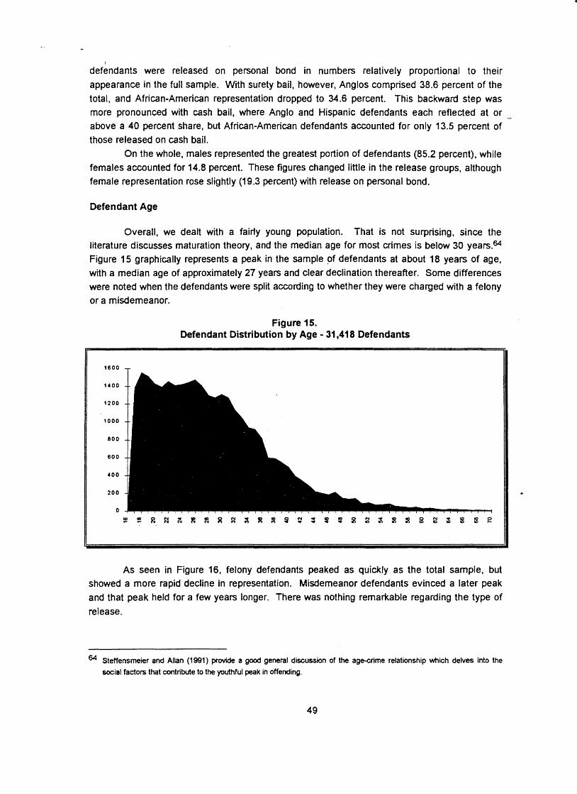
defkndants were released on personal bond in numbers relatively proportional to their appearance in the full sample. With surety bail, however, Anglos comprised 38.6 percent of the total, and African-American representation dropped to 34.6 percent. This backward step was more pronounced with cash bail, where Anglo and Hispanic defendants each reflected at or - above a 40 percent share, but African-American defendants accounted for only 13.5 percent of those released on cash bail.

On the whole, males represented the greatest portion of defendants (85.2 percent), while females accounted for 14.8 percent. These figures changed little in the release groups, although female representation rose slightly (1 9.3 percent) with release on personal bond.

Defendant Age

Overall, we dealt with a fairly young population. That is not surprising, since the literature discusses maturation theory, and the median age for most crimes is below 30 years? Figure 15 graphically represents a peak in the sample of defendants at about 18 years of age, with a median age of approximately 27 years and clear declination thereafter. Some differences were noted when the defendants were split according to whether they were charged with a felony or a misdemeanor.

Figure 15. Defendant Distribution by Age - 31,418 Defendants

As seen in Figure 16, felony defendants peaked as quickly as the total sample, but showed a more rapid decline in representation. Misdemeanor defendants evinced a later peak and that peak held for a few years longer. There was nothing remarkable regarding the type of release.

Steffensmeier and Allan (1991) provide a good general discussion of the age-crime relationship which delves into the axial factors that contribute to the youthful peak in offending.

Figure 16. Defendant Distribution by Age by Type of Offense - 31,418 Defendants

Fe bny

-.--..-..-..-. Msderneanor

Defendant Residence Situation

Defendant residence situation has for many years been thought to be important to the release decision and, ostensibly, to the likelihood of pretrial misconduct (e-g., Beeley, 1927). Whether one lives with immediate family or close relatives lies at the heart of the notion of "community ties."

Residence situations were split to a greater extent than was done previously at PTSA, in a way that would give insight into specific living arrangements. Of the entire sample, 78.7 percent of the responding defendants reportedly lived with family members; 23.9 percent lived with a spouse and/or children, and 54.8 percent with parents, siblings, grandparents, or other extended family members. An additional 18.9 percent were said to be living with friends at the time of arrest. This field had 7,440 missing values (23.7 percent of the total).

The above numbers held relatively true for defendants released on personal bond, but *

not so for surety and cash bail. The percentages for each with regard to defendants who lived with a spouse and or children rose to 33.6 percent and 41.3 percent of respondents, respectively. Both surety and cash bail descriptives indicated a level of missing values comparable to that of the entire sample.

With regard to the length of time at his or her current residence, the median time for the entire sample was 12 months. For all types of release, the median length of residence approached 24 months.

Economic Factors

Discussions of bail often touch upon class differences and financial ability; after all, in a system that relies upon monetary bail, one's financial ability to afford release can be extremely important.

I

Overall, 82.9 percent of defendants who responded when asked about employment indicated they were employed full-time. That figure rose for releasees, where full-time employment was reported by 85.3 percent of those released on personal bonds, 89.4 percent of those released on surety bail, and 92.1 percent of those released on cash bail. In the full - sample, this field had 14,659 missing values (46.7 percent). As we pointed out earlier, this field is among several which do not require a response to be entered and/or a response in another field on the same interview renders a response to this field unnecessary.

Looking at responses as a percentage of all interviews, 44.2 percent of the study sample reported full-time employment, compared with 55.8 percent for personal bond, 57.5 percent for surety bail, and 70.1 percent for cash bail. In each instance, fewer than 10 percent of any group reported part-time employment. In the released groups, missing value figures ranged from 23.9 percent for cash bail to 34.6 percent for personal bond.

Defendants in the study sample reported a median monthly income of $866.00 ($200.00 per week), 'and 90th percentile earnings were $1948.50.~~ Persons released on personal bond had a similar median income, but their income was $1732.00 per month at the upper end. Surety and cash bailed defendants reported median incomes of about $250.00 per week, but their incomes at the 90th percentile rose to $2,165.00 and $2,500.00 per month, respectively. Within the limits of the data, there is the suggestion of a relationship between income and ability to secure financial release, but this bears further examination.

A similar suggestion arises in looking at reported spousal income. Although the median spousal income per month for all groups was $0.00, 90th percentile income rose as one moved toward purely financial release. The upper spousal income for both the study sample and those released on personal bond was $1,299.00 per month, with an increase to $1,515.50 for those on surety bail, and another to $1,800.00 per month for persons on cash bail. Because the missing values comprised approximately 77 percent of each group, this will also remain a direction for further inquiry.

Financial resources again appeared in the guise of monthly rental or mortgage payments. The median figure for both the study sample and those released on personal bond was $100.00 per month, with upper end figures of $365.00 and $375.00 per month, respectively. The median payment for persons released on surety bail was $200.00 per month, topping out at $420.00 per month. Persons released on cash bail reported a median payment of $230.00 per month, with payments of $500.00 per month at the 90th percentile.

Defendant Alcohol and Drug Problems

Study defendants did not acknowledge any problems with alcohol or dnrgs in numbers that begin to approach the numbers of DUI arrests or arrests for possession of small amounts of crack cocaine. The highest figures appear in the full sample, where 3.3 percent of the total reported an alcohol problem and 3 percent reported a dnrg problem. Speculation suggests that

65 In most distributions, focusing on figures at either extreme tends to give a rather distorted view of reallty. The 90th percentile figure was chosen because it provides a better picture of earnings at the upper end of the distribution. For example, if in this instance we had chosen the most extreme income figure, we would tell you that at least one defendant reported earnings of $3,043,969.56 per month. Howwer, we know that a number of that magnitude likely resulted either from a data entry error at interview or an incorrect earning period indicator (perhaps using WK" instead of YR").

I

defendants feel an affirmative response to either question would reflect badly, and perhaps impact their chances for release on personal bond or their bond amount. In that case, officials may want to investigate presumptive indicators of drug use, instead of reliance on self-reports (see Goldkamp et al., 1990). -

Criminal history

Defendants in the study sample were not well acquainted with the justice system. Of the responses available, 61.5 percent of the defendants had no prior felony convictions and 46.5 percent had no prior misdemeanor convictions. If we expand that to permit one conviction, the figures rise to 80.2 percent and 68.4 percent, respectively. Of the defendants with prior convictions, 10.1 percent were on probation at the time of arrest and 19.5 percent were on parole. A verified failure to appear was found for 7.7 percent of the respondents, and the existence of unexecuted (open) warrants posed a problem for less than 6 percent of the defendants.

Pretrial release policies can easily be seen in the histories of the defendants who were released on personal bond. Available data indicate that 95.6 percent of these persons had no prior felony convictions and 94 percent had one misdemeanor conviction or less. At the time of interview, 1.8 percent were on probation at the time of arrest and 0.9 percent were on parole. A prior failure to appear was a factor for only 2 percent of the respondents, and the percentage of defendants with open warrants did not exceed 5 percent.

Persons who were released on surety bail resembled the whole of the study defendants in most respects. Seventy point two percent of the respondents had no prior felony convictions and 45.5 percent had no prior misdemeanor convictions. Expanding that to allow one prior conviction would push the figures to 86.6 percent and 69.4 percent, respectively. Among these defendants, 11.4 percent were on probation at the time of arrest, and 11.6 percent were on parole. A verified failure to appear was found for 8.2 percent of the respondents, and open warrants posed a problem for less than 5 percent of the defendants.

Finally, we look at the defendants who were released on cash bail. The data reflect that 90.9 percent had no prior felony convictions and 66.4 percent had no prior misdemeanor convictions. A combined total of 6 percent were on probation or parole at the time of arrest. Only 2.2 percent of the respondents had a verified prior failure to appear, and fewer than 1.5 percent of these persons had outstanding warrants.

Conclusion

A final task in this section is to relate the outcome of the various types of release according to what we have been able to glean from JlMS data on 8,166 defendants for whom data was near-complete. Not surprisingly, cash bailed defendants performed the best, with 4.8 percent failing to appear and 2.9 percent reoffending.

Curiously, personal bond releases and surety bail releases reached similar ends. The data indicate that 14.7 percent of the defendants released on personal bond through PTSA engaged in misconduct; 10.8 percent failed to appear and 3.9 percent engaged in criminal

I

activity while on bond? Surety bailed defendants fared only slightly better at 14.1 percent; 9.2 percent failed to appear and 4.9 percent committed new offenses. If it holds true that there is no substantial difference in outcome between personal bonds and surety bail, then officials may wish to embrace release through personal bonds. This method would at least hold the potential - for more accurate prediction combined with the ability to set conditions and monitor compliance.

66 The figure for PTSA releases does not include data on 21 defendants released on personal bond through their respective courts without agency supervisii. These 21 defendants included one case in which the defendant failed to appear, and

the inclusion of these case would cause a negligibk increase in the personal t m d misconduct rate to 14.6 percent.

Section Five lnstrument Development and Testing

The Findings

In applying the methods discussed in the previous section to the data, we first evaluated the existing (hereafter "former) instrument in the way that it was being used. This established a basis for assessing the relative merits of new models. Clearly, if a new instrument does not show improvement over what is currently in place, there is no need to undergo the expense and effort of changing current practices. The following discussion explains the findings and our procedures in evaluating the former instrument and in exploring alternative prediction models.

The Former Instrument

At the time this study was undertaken, the instrument in use by PTSA combined six items reflecting community ties and FTA history with the defendant's prior criminal record to produce a risk score. The items were based upon the Vera point scale developed in New York in the 1960s.

The defendant's response to each of the items on the instrument was scored according to the point scale shown in Figure 17. The point total ran from a high of 7 points to a low which was determined by the prior criminal history of the defendant. For this analysis, the low score was -22. Scores of 4 or higher were considered eligible for presentation to the judges as potential candidates for a personal bond. From this we inferred that defendants meeting that criterion were thought to be better risks thanthose who scored less than 4 points.

Figure 17. Fonner Bail Classification Items and Scoring

11 Resides in cwntv - --- - - - - --

Telephone in home Whom defendant lives with

" Length of residence Employment Prior FTA Prior convictions

+1 if defendant lies in Hams County. +1 if true. +1 if def. lives with parents, spouse andlor children + I if 1 year or more + l if fulVpart time employed, disabled, or homemaker +1 if defendant had no prior failures to appear -1 for each prior felony and misdemeanor, with the first misdemeanor waived,

I + I if no priors or 1 prior misdemeanor 11

The former instrument was scaled so that lower scores denoted higher risk. This can be seen in Figure 18, where the failure rates generally trend from high to low across defendant classes. The first category consisted of all negative scores; combining them was necessary since there were so few cases. Groups <O, 1, 2, and 3 were small, each representing from 3 to 6 percent of the population.

Figure 18. Distribution of Failures by the Former

Instrument Classification Score

I1 Score I Number of 1 Number of 1 Total I Failure Rate I Percent of I1 Successes Failures Population

< 0 1 37 29 1 66 0.175 2.44%

I I I

I Total I 755 ) 6,796 1 0.111 (

Figure 19. Failure Rates by Defendant Classification

on the Current Risk Assessment Instrument

Failure Rate 1 0.3 T R


Figure 19 graphically depicts the distribution of risk across defendant groups. With the exception of the first two categories, the graph shows a general downward trend as the classification scores increased. The second category (defendants scoring 0) appeared to be more related to categories 6 and 7 (scores of 4 or 5) than it was to categories 1 and 3 (scores of - 1 or 1). It is also apparent from the graph that there were several categories that had relatively few cases, which made the confidence interval wider. Only the lowest-risk group (scores of 7) fell clearly below the average failure rate for all groups (the base line). All other groups included the average as part of their respective confidence intervals. This suggests that the instrument did not differentiate cases on the basis of risk very well.

Figure 20 shows the mean cost rating (MCR) information (see Appendix B for a cursory explanation of MCR computation). With a rating of 0.1635, the model was confirmed to have

mikmal predictive capability; that is, the model improved prediction by about 16.3 percent of the total possible improvement over the base rate. Even this may be overstated, in that the classification efficiency rating method used here (MCR) is insensitive to order. If it is assumed that risk is associated linearly with a score (i.e., the lower the score, the greater the risk), the - instrument actually performed below indicated levels.

Figure 20. Classification Efficiency of the Former Model

Score Frequency * J

0.0942 0.3731 559 81 0.0925 0.1 073

0.1 495 0.5226 885 131 0.1 46!5 0.1 735 '

0.2237 0.7463 1,378 1 42 0.2281 0.1 881

0.2538 1.0000 1,602 1 23 0.2652 0.1 629

Base Rate 0.1 11 1 Mean Cost Rating 0.1635 If .

The primary problem with the former instrument was that there was no balance between factors that were more influential and those that were less so; all factors were weighted equally in arriving at a total score. However, one may have cause to question whether having 5 prior convictions makes a defendant half as risky as one with 10. One may defendant with one prior felony and a telephone poses the same risk as a telephone.

The Reweighted Instrument

likewise wonder if a first offender with no

The problems identified with the way in which the former instrument combined factors to arrive at a classification score could be addressed by weighting each factor according to its relative importance in predicting pretrial misconduct. By assigning more weight to having prior felonies than to having a telephone, the problem described in the previous section could be resolved. It may be that all else being equal, owning a telephone may be predictive of pretrial behavior, but what role does it play with all else is not equal? This is where logistic regression comes in. We evaluated the items in use to determine which of them were indeed predictive of pretrial misconduct, and derived weights to maximize our ability to classify defendants according to the risk they represent.

Correlation

The first step was to examine the bivariate relationships between the criterion and predictor variables. In this instance, a correlation matrix provides us with a look at how the variables interrelated. The correlations are presented in two stages which address two separate but related questions. The first stage examines the relationship between the predictor variables

I

and three ways of measuring failure. The second examines the predictor variables themselves.

interrelationships between the

73e Relationship Between Predictor and Criterion Variables

Figure 21 shows the correlations between the predictor items and failure to appear, rearrest, and the combination of these called misconduct. As we discussed earlier, correlation coefficients range from -1 to 0 to +I, indicating the strength and direction of a linear relationship between two variables. Coefficients showing a negative sign are inversely related to the failure rate; that is, as the value of the related variable increases, the likelihood of failure decreases. Likewise, those without a sign are positively related, so that the higher the predictor score the higher the likelihood of failure.

Two predictors represented combinations of other variables found in the matrix. PRIOR CONVICTIONS was composed of PRIOR FELONIES and PRIOR MISDEMEANORS, with the first misdemeanor conviction (if any) removed. TOTAL represented the point score derived from the listed factors as described in the previous section. .

The relationships with each of the predictor variables had the same sign for both FTA and REARREST. This means that changes in the predictor values affected the likelihood of FTA and REARREST in similar ways; there were no factors that increased FTA rates while reducing REARRESTS. That enabled us to combine the two outcomes into a single measure (MISCONDUCT) without added complications. This also served the agency's interests in reducing risk assessment to a single instrument. Based on this finding, we limited further analysis to MISCONDUCT as the criterion variable.

Figure 21. Correlations Between the Fonner Instrument Items and

Failure to Appear, Rearrest, and Misconduct

1 Scale ttm I FTA I REARREST 1 MISCONDUCT ]I

The matrix shows that there were imbalances in the instrument as it was then implemented, in that TOTAL had a lower correlation with misconduct than PRIOR FELONIES or EMPLOYMENT (PRIOR CONVICTIONS can be included in this group but is largely redundant with PRIOR FELONIES). What this told us was that either of these two predictors alone makes as good an indicator as, or a better indicator of, misconduct than all the items taken together in an unweighted score.

' Resides in County Telephone in Home

j Whom lives With

-.O040 1 -.0148 - . O m 1 -.0217

-.Ol11 -.0800'

- . O m ) -.0029 -.0242'

The Interrelationships Between Predictor Variables

While the correlation between the criterion and predictor variables was critical to determining the fitness of individual variables for predicting outcomes, it was also important to - explore the degree to which the predictor variables interrelated with each other. Too much similarity (high correlation) between these variables weakens their ability to make accurate and reliable predictions. Table 22 shows the interrelationships between predictor variables.

Many of the items were highly intercorrelated, scoring from .300 and higher. This suggests that much of the correlation between these factors and misconduct was coming from common sources and would not add together to greatly increase the power of the final prediction model.

Figure 22. Correlations Between Predictors Used in

the Fonner Risk Instrument

Of particular concern were the high correlations between items 1 through 6. Should these items be entered into a single regression model, they would conflict somewhat. This would cause the weaker predictor to drop out, being regarded as insignificant by the regression procedure. This does not mean that a predictor does not really predict; rather, it means that other predictors in the model are doing the same job a little better, and the dropped predictor is not needed. Consequently, it is not unusual for an analysis to lose variables that everyone thought (or knew) to be important.

Logistic Regression

The variables were entered stepwise into a logistic regression model. Two minor changes were made to the way in which these factors were applied. First, PRIOR FTA was scored if the defendant had a failure to appear on his or her record. Second, all misdemeanor convictions were calculated, and the first was not waived. Six of the eight factors were found to be significant. Whom lives with and lengfh of residence were found to be redundant and were dropped from the equation. The remaining factors were found (with 95 percent certainty) to contribute to predicting pretrial misconduct.

Figure 23. Logistic Regression Estimate and Transfomed Scores

for the Reweighted Classification lnstrument

The regression coefficients were transformed into integers by dividing them by .4084. As a general nde applied in this study, this constant was established as being two times the smallest coefficient. In this instance, PRIOR MISDEMEANORS would normally be applied, but this was deemed to produce excessively large weights. Therefore, the next smallest coefficient (PRIOR FTA) was applied, which was .2042. The regression coefficients were divided by the constant and rounded to their nearest integer value to produce the model weights.

Classification h

We applied the weights in Figure 23 to the data and generated a table disaggregated by classification score. Figure 24 shows the distribution of failures for each of the classes. Those classes that did not have sufficient numbers of cases to yield interpretable results were combined with other classes. Of the 6,796 cases classified, 89 fell above a score of 2. These were combined with the "2" class. Due to the open-ended treatment of prior offenses, there were 21 1 cases that distributed themselves from a score of -6 to -26. These were combined with the class shown as "-5 or less."

Figure 24. Distribution of Failures by the Reweighted Instrument Classification Score

I( Score 1 Number of I Nwnber of I Total 1 Failure Rate I Percent of 1

2

Figure 25 shows the failure rate, confidence intervals, and proportion of the population for each class. The graph emphasizes the similarity between the groups scoring -1, -2, and -3.

Successes 2,015

r 111

222

6,041

-4

-5 w less

Total

Failures 150

35

74

755

2,165

146

296

6,7%

0.069284

0.239726

0.250000

0.1 11095

Population 31.86

2.1 5

4.36

100.00

' A

I

In the long run, it is doubtful if there would have been any substantial difference in the failure rates of these three classes.

Figure 25. Failure Rates by Defendant Classification on the Reweighted Items of the Fonner

Risk Assessment lnstrument

0 0.1 0.2 0.3 0.4 0.5 0.6 0.7 0.8 0.9

Proportion d the Population

The reweighted scale also showed substantial improvement in its mean cost rating, as seen in Figure 26. The reweighted items increased the predictive power of the former model by 46.7 percent over the way in which it was previously implemented (from .I635 to .2398). This represented a substantial improvement in predictive power, yet the model was based upon only six of the original eight items.

Figure 26. Classification Efficiency of the Reweighted Items Used in the Former Instrument

Score ( Frequency

1,421

Total 3.21 0

Proportion 1 P(Cwn) 1 Freq Succ ( Freq Fail 1 P(Success)

2,735 475

Base Rate 0.1 11 1

I Mean Cod Rating 0.2398

In conclusion, these results indicated that the existing classification factors could be "fine tuned" to produce improved results over the way in which they were used. Unfortunately, even a

I

reweighting of the items would not save the agency the cost of reprinting interview forms or retraining staff. The changes required to adopt the reweighted instrument would not be substantially different from those necessary to adopt an entirely new model.

.. . . - New Instrument Development

lnstrument development refers to the process of evaluating available data to determine which combination will render the best prediction of pretrial misconduct. It is not simply a matter of finding those items that have substantial interrelatedness with misconduct; rather, the interrelatedness of the predictors must also be taken into account. Ideally, the final model will consist of predictors that are substantially related to the outcome (criterion) measure while not being highly interrelated with other predictors. Interrelatedness among the predictor variables indicates that they measure the same portion of the variation found in the criterion variable and perhaps fail to adequately cover other portions. This results in a model with a very narrow base which, like a seesaw, can dramatically change orientation with relatively minor influences. These are unstable models and are among the least desirable for instrument development.

The process of developing a stable and predictive model is not a simple one-step operation. Variables must be examined in a variety of combinations to determine which work together to bring about the dekired ends. This section discusses the process used in this study to devise a prediction instrument and then details the findings that led to the proposed instrument.

Testing the Specific Offense Categories

One of the central issues in defendant classification is the extent to which the offenses with which defendants are charged relates. to the likelihood of pretrial misconduct. It is well known that certain kinds of offenders commit crimes at greater rates than do other offenders. Likewise, certain offenses carry different penalties or stigmas that may prompt defendants to take flight. It therefore seems logical that the nature of the offense may be important to gauge the likelihood of pretrial misconduct.

To test the impact of offense on the likelihood of pretrial misconduct, the primary (most serious) offense for each pretrial releasee was coded into 16 categories. These are shown in Figure 27 along with their frequencies among released defendants. Again, we must emphasize

0

that this inquiry deals with those defendants who were actually released in some f o m or fashion during their pretrial period. It does not and should not be taken to reflect the distribution of offenses charged in Hams County.

These offense categories were added as special variables to the data set so that their impact could be individually studied. For each of the offense categories, a variable containing either a 0 or 1 was added to each defendant record. A zero indicated that the defendant was not charged with the designated offense as a primary charge, a one indicated that the designated charge was the primary offense. If defendants belonging to any of these offense categories were more or less likely to fail on pretrial release, our statistical analysis would show the offenses to be significantly related to misconduct.

Figure 27. Offense Categories and Their Frequencies

- - for Released Defendants :; ., '. ++ .

I - -

Traffc Offenses 9.91)

I1 Trespassing 1 174 1 2.60 I I Robbery 1 0.24 )1

Weapons Vdations - Assault

Other Property Other Personal

479 1 7.15 ' 298 I 4.45

Murder 7 0.10 Auto Theft 43 0.64

Missing Data 94

Categorizing Variables

In the evaluation of the former and reweighted former models, we saw the difficulties I that come from open-ended factors, such as PRIOR MISDEMEANORS. The wide range of

scores these items acquire cause the instrument to spread cases so thin as to produce dozens more categories than can be filled with enough cases to produce meaningful results. One way to avoid this is to find appropriate break points, where scores beyond a certain point are assigned a single score. The problem-in doing this is finding the prop& break point.

To aid in finding the appropriate break point, we computed the failure rate for individual - - - - - - - - - - - gmups o fmtegoka l va"ables. For continuous vahables, such as age, we attempted to break

the ages into segments that would limit the number of categories to* a manageable number, while allowing maximum freedom for the failure rate to vary between the groupings. The purpose of this effort was to group the data in ways that maximized the differentiation of the failure rate, while maintaining a logically consistent coding scheme. w

Figure 28 shows the categories and failure rates for age. In general, 2-year age cohorts were used, the exceptions being either extreme. The first category combined ages 16 through 18 years, while the last combined all persons of age 35 and over. The failure rates by age cohort showed that ages 16 through 20 yielded the highest pretrial failure rates (14.08 percent and 17.46 percent, respectively). The 21-22 year age cohort was marginal (12.40 percent), with a general drop to the high 9- and low 10 percents. The 25-26 year group showed a failure rate of 13.83 percent, which ran contrary to the general trend. Nevertheless, it appeared as if the break point occurred around age 20. Adopting this as a break point appeared to maximally differentiate high and low failure rates based upon age. It also bore intuitive appeal, as age 21 represents the traditional age of majority. If the defendant was below 21 years of age, YOUNG was coded I. If the defendant was 21 or older, YOUNG was coded 0.

Figure 28. Failure Rates for Defendants Classified by Age

When examining the failure rates for the classes of defendants based on their living arrangements (Figure 29), two groups stood out as having the lowest failure rates. Defendants living with a spouse and/or children, or the defendant living alone, both showed failure rates of some 7 percent in contrast to the 10 percent to 30 percent found in other groups. The responses of SeH or Spouse and Children were coded together as a new variable called NUCLEAR for nuclear family.

Figure 29. Failure Rates by Category of HRL

(Who does the defendant live with?)

Education is thought to be the great equalizer. Indeed, we found that most defendants had an almost equal failure rate across levels of education, as shown in Figure 30. The exceptions were the none to 0 years category and the two categories pertaining to college. The . two college categories were combined to make EDUCAT equal to 1. all other categories were coded 0.

Figure 30. Failure Rates by Category of Response to the

Defendant's Highest Level of Education

I1 Domestic from 1 to 6 years 1 .112500 II

- - - -

Category Missing

The number of prior felonies was a major category in the former model analysis.

-

Failure Rate

However, it posed a problem by creating an open-ended category, where a small number of

I+ None to 0 years

defendants could stretch the distribution beyond practical limits. The analysis of defendants with 0 through 10 prior felony convictions is shown in Figure 31. Keeping in mind that the numbers of cases fall off rapidly after about the fourth felony, we saw that there was something of a pattern taking shape. The failure rates for 0 and 1 felony (9.87 percent and 12.34 percent) were fairly similar, whereas the failure rates for 2, 3, and 4 felonies ran at roughly 24 percent. By dichotomizing the distribution with 0 and 1 convictions in the "low-risk" category and 2 or more convictions in the "high-risk" category, most of the predictive power of prior felonies could be captured in the variable we call PF, for prior felonies. This variable consisted of a value of zero for 0 or 1 prior felony, and a value of 1 for 2 or more felonies.

Figure 31. Failure Rate by Number of Prior Felonies

Following the same form for misdemeanors as for felonies, we saw that a similar picture emerged (Figure 32). Zero and one misdemeanors related to a failure rate of 10.25 percent and 9.84 percent, respectively. The greater number of misdemeanors showed higher rates of failure, but not in a substantial progression.

Figure 32. Failure Rate by Number of Prior Misdemeanors

Figure 33 shows that the failure rate among US. citizens was somewhat greater than among aliens. While this may run counter-intuitive, one must remember that this is a sample of released defendants. If there is substantial belief that an alien defendant may make a run for the border, there is little doubt that this person would be unlikely to attain release. This would influence the failure rates that would be shown here. his variable was recoded so that U.S. citizens were recorded as 1s. Aliens were recorded as Os.

Figure 33. Failure Rate by Citizenship Status

Another assumption concerning community ties is that a person with dependents will be more likely to fulfill his or her obligations. Once again, a pattern emerged where the persons with 0 or 1 child appeared to be more likely to fail than those with more children (Figure 34). Once again, the number of cases in each category should be seen as a determinant of the reliability of the results as each level.

Figure 34. Failure Rate by Number of Children

Residing in the Household

Number Failure Rate 0 .I26792 1 -1 181 29

We assumed that residents of Hams County or contiguous counties would be less likely to fail, seeing how a court appearance is made much simpler for them, and the risks of failing to appear seem much greater. Yet we found that the "ALL OTHER" category had the best failure rate of all (Figure 35). This may have been due to the decisionmaking processes associated

I

with release. Due to the greater distance from home to court, outsiders who may appear marginal may not be released whereas a local person may be considered-all else being equal. Those who resided in Hams or contiguous counties were given a 1 on this item, the ALL OTHER category was scored 0. -

Figure 35. Failure Rate by County of Residence

Contiguous I .I34694 All Other .067227 I

This concluded the categorizing phase of the analysis. These and the other variables in the data set, many of them already dichotomous, then were evaluated on the basis of their correlation with the criterion variable misconduct (MISC) and with other predictor variables in preparation for building an alternative model.

Means, Standard Deviations and Correlations

The search for a new model involved some 68 variables in all. Some represented modifications of others in the analysis. The variable PM, for example, represented the recoded p io r misdemeanors, as was discussed in the previous section. As such, the two variables could not be used in the same logistic regression model, but both were evaluated in the correlation analysis so that the loss of predictive power due to recoding could be evaluated.

A major consideration when selecting variables is that there are few missing values. In general, when a statistical procedure encounters a variable that is missing a value, the entire case is eliminated from the analysis. A large number of missing values can rapidly decimate a sample, particularly if a large number of variables are involved. For this reason, YRD (defendant-reported disabilw and GED (completion of high school equivalency program) dropped from the analysis. YRD had only 148 non-missing cases and GED had 4.146 cases missing.

Based upon an examination of the correlation matrix, the following variables were tested: VET (veteran status), HSG (high school graduate), HEA (reported health problem), ALC (reported alcohol problem), PWD (reported drug problem), AUTl (ownership of auto), PFTA @nor failures to appear), N l T (Hamk County address), N2T (telephone in residence), N3T ( who lives with, similar to HRL) , N4T (length of residence in Harris County), N ST (employment status), N6T (another measure of p io r failures to appear), PPRO (pmbation status), PPAR (parole status), AHCW (open local warrant), AFUG (other open warrant), and the 1 5 recoded offenses. From the previous section, the recoded PF @nor felony convictions), PM @nor misdemeanor convictions), NUCLEAR (whether defendant lives with spouse andlor children), YOUNG (under age 21), CONC (county of residence), EDUCAT (level of education), NOCL (number of children in residence), and USC (citizenship status) were added. In all, 40 variables were tested using logistic regression.

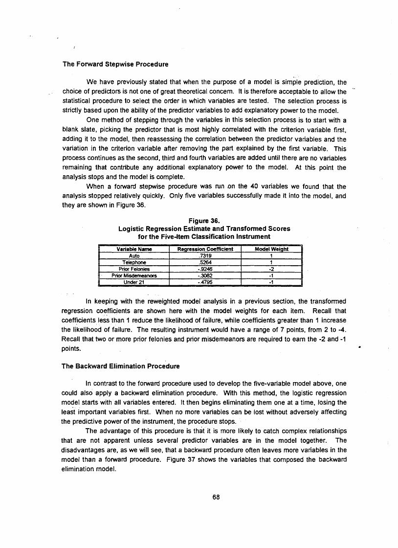
The Foward Stepwise Procedure

We have previously stated that when the purpose of a model is simple prediction, the -

. , choice of predictors is not one of great theoretical concern. It is therefore acceptable to allow the statistical procedure to select the order in which variables are tested. The selection process is strictly based upon the ability of the predictor variables to add explanatory power to the model.

One method of stepping through the variables in this selection process is to start with a blank slate, picking the predictor that is most highly correlated with the criterion variable first, adding it to the model, then reassessing the correlation between the predictor variables and the variation in the criterion variable after removing the part explained by the first variable. This process continues as the second, third and fourth variables are added until there are no variables remaining that contribute any additional explanatory power to the model. At this point the analysis stops and the model is complete.

When a forward stepwise procedure was mn .on the 40 variables we found that the analysis stopped relatively quickly. Only five variables successfully made it into the model, and they are shown in Figure 36.

Figure 36. Logistic Regression Estimate and Transformed Scores

for the Five-ltem Classification Instrument

In keeping with the reweighted model analysis in a previous section, the transformed regression coefficients are shown here with the model weights for each item. Recall that coefficients le& than 1 reduce the likelihood of failure, while coefficients greater than 1 increase the likelihood of failure. The resulting instrument would have a range of 7 points, from 2 to -4. Recall that two or more prior felonies and prior misdemeanors are required to earn the -2 and -1 points.

The Backward Elimination Procedure

In contrast to the forward procedure used to develop the five-variable model above, one could also apply a backward elimination procedure. With this method, the logistic regression model starts with all variables entered. It then begins eliminating them one at a time, losing the lea& important variables first. When no more variables can be lost without adversely affecting the predictive power of the instrument, the procedure stops.

The advantage of this procedure is that it is more likely to catch complex relationships that are not apparent unless several predictor variables are in the model together. The disadvantages are, as we will see, that a backward procedure often leaves more variables in the model than a forward procedure. Figure 37 shows the variables that composed the backward elimination model.


for the Nine-Item Classification lnstrument

I Variable Name Regression Model Weight Cafficient

Auto I S310 +I Prior Felonies -.W 3

There were nine items in this instrument, with scores potentially ranging from 4 to -1 1. The five items of the forward stepwise model can also be found in this model, but with the addition of employment, prior FTAs, nuclear family, and the offense of trespassing.

Curiously, 14 of the 15 offenses were dropped from the model. This suggests that while certain offenses are correlated with failure rates, these correlations may be better explained by other factors in the model. Auto theff may be linked with pretrial failure, for example, but then auto theft is typically a young man's crime. If YOUTH is a strong enough predictor, it could override the effects of auto theft and cause the offense category to be dropped from the model.

As a matter of practical consideration, this model raised the issue of whether keeping the offense of frespassing as a predictor was appropriate. While statistically significant, trespassing might be difficult to defend from a logical point of view, considering that it was the only offense category to survive the backward elimination process. Whether significant or justifiable, the underlying question was whether its exclusion would adversely impact the ability of the model to predict misconduct.


for the Eight-ttem Classification Instrument

After removing trespassing, the logistic regression results indicated that most of the coefficients of the remaining items were not changed substantially. Figure 38 shows the regression coefficients and the weights assigned to each of the eight items. The most substantial change was the increase of 0.1045 in the PRIOR FTAs coefficient (from -.3920 in the 9-Item model to -.4965 in the eight-item model), indicating the possibility that there were a disproportionate number of trespassers who had a record of prior failures to appear.

Variable Name Auto

Prior Felonies-

t Employed, school or homemaker

Under 21

Regression Coefficient .5168 -.9111 3383 - 3 0 7

Model Weight 1 1 -2 1 -1

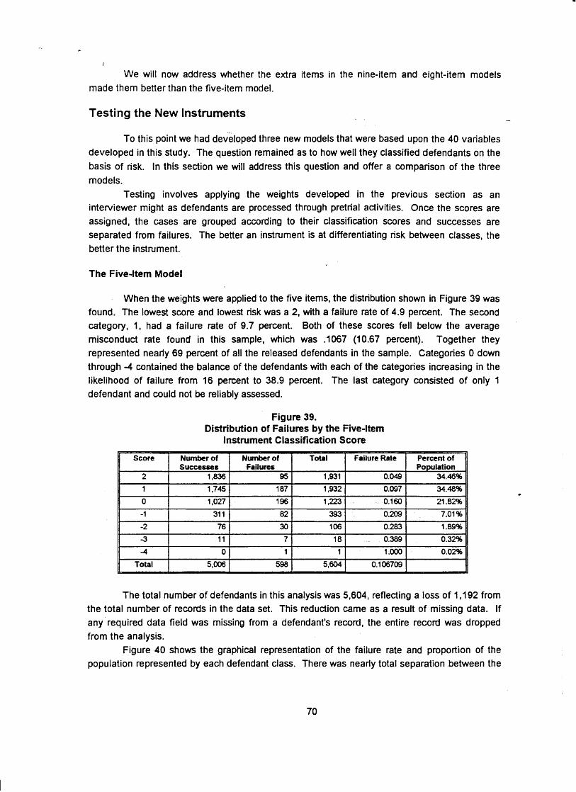
1

We will now address whether the extra items in the nine-item and eight-item models made them better than the five-item model.

Testing the New instruments -

To this point we had developed three new models that were based upon the 40 variables developed in this study. The question remained as to how well they classified defendants on the basis of risk. In this section we will address this question and offer a comparison of the three models.

Testing involves applying the weights developed in the previous section as an interviewer might as defendants are processed through pretrial activities. Once the scores are assigned, the cases are grouped according to their classification scores and successes are separated from failures. The better an instrument is at differentiating risk between classes, the better the instrument.

The Five-Item Model

- When the weights were applied to the five items, the distribution shown in Figure 39 was

found. The lowest score and lowest risk was a 2, with a failure rate of 4.9 percent. The second category, 1, had a failure rate of 9.7 percent. Both of these scores fell below the average misconduct rate found in this sample, which was ,1067 (10.67 percent). Together they represented nearly 69 percent of all the released defendants in the sample. Categories 0 down through -4 contained the balance of the defendants with each of the categories increasing in the likelihood of failure from 16 percent to 38.9 percent. The last category consisted of only 1 defendant and could not be reliably assessed.

Figure 39. Distribution of Failures by the Five-Item

Instrument Classification Score

The total number of defendants in this analysis was 5,604, reflecting a loss of 1 ,I 92 from the total number of records in the data set. This reduction came as a result of missing data. If any required data field was missing from a defendant's record, the entire record was dropped from the analysis.

Figure 40 shows the graphical representation of the failure rate and proportion of the population represented by each defendant class. There was nearly total separation between the

- I

upper confidence interval of a lower group and the lower confidence interval of the upper for the largest three groups. This assured that the rate developed for each of these groups was distinct from the others and in the long run should remain distinct as more cases are added to the pool. Only the two "high-risk" groups shown (scores of -1 and -2) seemed to overlap substantially. - This was due in part to their smaller group size. Figure 40 does not show the two smallest groups (scores of -3 and -4) because together they represented less than 1 percent of the total defendant population. This serves as a reminder that results coming from small group sizes cannot be counted on for accuracy in the long run.

Figure 40. Failure Rates by Defendant Classification

on the Proposed Five-ltern Instrument ppp ---

6 k r e Rate

0 0.1 0.2 0.3 0.4 0.5 0.6, 0.7 0.8 0.9


Figure 41. Classification Efficiency of the Items Used in the Five-Item Instrument

Mean Cost Rating

I

Computing the classification efficiency of the five-item model, we found that the model improved prediction by about 32 percent of the total possible improvement (0.3199); this represented a net of 95.6 percent improvement over the former model. Figure 41 details this analysis. -

In sum, the strength of this model was improved classification efficiency over the former and reweighted former instrument. It required fewer items than any other tested model and was composed of items that had a certain degree of intuitive appeal. The lack of certain items, such as PRIOR FTA may be disconcerting to some, but consider how few people PRIOR FTA actually covers, and consider further that to have a prior failure to appear one most likely has a prior felony or misdemeanor conviction. The strength of these latter two measures overpowers the less likely event of FTA.

The Nine-Item Model

The nine-item model divided the defendant population into 12 groups, ranging from 4 to -7. One noticeable feature of this model was that the percent of the population, shown in Figure 42, was more finely distributed than with the other models examined in this study. This is understandable in that the number of groups will be determined by the number of items in the scale. The more items, the more groups, and (in most cases) the better the distribution of cases within the groups.

Figure 42. Distribution of Failures by the Nine-ltern Instrument Classification Score

I) Score 1 Number of I Number of 1 Total I Failure Rate S u c c e ~ s Failures

4 641 20 661 0.030


15.98%

20.09%

18.1 8%

With the exception of the group scoring a -3, the failure rate showed a fairly consistent increase as scores decreased. The failure rates of the groups scoring less than -3 represented a small and unstable set of parameters; the instrument would be well served by aggregating them.

The total number of cases in this analysis was 4,136; this represented a loss of 2,660 cases due to missing values. This does not undermine the study or its purpose, as long as the problem is remedied before a new instrument is implemented. Further consultation with PTSA staff will be necessary to team the nature of this problem and how it may best be solved.

I

The failure rates for each of the groups in the nine-item instrument are shown in Figure 43. Seven "levels" were clearly defined by this model. Two groups contained the base rate within their limits; the other five fell clearly above or below the base rate. There appeared to be

a strong linear pattern to the pla$ment of the "steps," unlike the previous~models -. q where there - appeared to be a "hook" on the high risk end of the scale.

Figure 43. Failure - - - Rates by Defendant Classification

on the Proposed Nine-Item Instrument

Failure Rate

0 45

Proportion of thc Population

The mean cost rating of the instrument, shown in Figure 44, was somewhat disappointing in light of the larger number of variables. For all practical purposes, it was only slightly better than the five-item model, having a mean cost rating of .3387.

Figure 44. Classification Efficiency of the

Score

Total

Proposed Nine-Item Instrument

752 0.1 81 8 0.6393 672 80 0.1 832 0.17131

831 0.2009 0.6402 777. 54 0.21 18 0.1 156

661 0.1 598 1.0000 641 20 0.1747 0.0428

4,136 3,669 467 I, Base Rate 0.1 129 1 Mean Cod Rating 0.3387 I

In sum, the nine-item instrument was equal in efficiency to the five-item instrument, however, it offered more groups with a more graduated scaie of risk than did the other instruments.

The Eight Item Model

The eight-item model established 9 groups with scores ranging from 4 to -4. While containing fewer categories than the nine-item model, the failure rates per group showed a strong progression from a low of 3.1 percent to a high of 50 percent. Notably, the rates below a score of -2 were less stable due to the small number of cases.

Figure 45. Distribution of Failures by the Eight-Item Instrument Classification Score

Score 1 Number of I Numkr of I Total ( Failure Rate I Percent of 11 Successes Failures Population

4 742 24 766 0.031 332 1 1.27%

3 1.473 92 0.058786 23.03%

Total 6,041 755 6.796 1 0 . 1 1 l M

I

Figure 45 shows the distribution of failures according to defendants' scores on the eight- item instrument. Those scoring 4, 3 or 2 represented risks below the then-current level of Al l (1 failure in 9), while those falling from 1 to -4 represented above-average risks. About 58 percent of the entire released population fell in the three lowest-risk categories. Moreover, of the 755 - observed failures, 279 (36.95 percent) were by persons in the low-risk group. This suggests that nearly two-thirds of the total pretrial failure risk is represented by less than one-half of the entire released population.

Figure 46. Failure Rates by Defendant Classification on the Proposed Eight-Item Instrument

I . - , Figure 47. ~lassif ickon EPficiency of the Proposed Eight-Item Instrument

1 1 I

4 766 1 0.11271 . 1.0000

Total 6,796

Freq Succ Freq Fail

H B a a Rate 0.1111 II 11 Mean Cost Rating - . 0.3251 11

The failure rates for each of the groups are shown in Figure 46. In comparing this model to the 9-item model, we found that there were seven steps shown in both graphs. This was due to the small number of cases falling into the highest-risk categories. Those categories which represented less than 1 percent of the total sample are not shown on the graph. The confidence intervals appear to be narrower in the 8-item model when compared to the 9-item model

I

because there are fewer groups (9 groups compared to 12 for the 9-item model) over which the cases were spread. More cases result in greater predictive power, and therefore narrower confidence intervals.

The mean cost rating of the &item model, shown in Figure 47, was about the same as - that for the 9-item' model (.3251,: compared to .3387 for the 9-item model). This does not represent a meaningful difference with respect to the performance of these models in actual use over an extended period of time.

Interaction Effects Models , ? . 2 .

Before concluding this section, we feel it is important to note that a number of other analyses were performed that are not being brought into this discussion. One of those areas involved evaluation for interaction terms. An interaction t e n is a variable that is entered into the

"egression model that expresses a dependency of one variable on another. For example, assume young men are more likely to be rearrested than older men. But perhaps older women are more likely to be rearrested than' younger women. If one were to ask "Who is more likely to be rearrested. a younger or older person?" The answer would be "It depends whether you are referring to men or women."

While interaction terms pervade much of criminal justice studies, we found only minor (and largely nonsignificant) traces in the present work. The main effects models we have developed here are not subject to improvement by introducing the complications of interaction terms.

. Conclusions :.. - , . ,

.- -

In conclusion, we presented four models for bail classification. The former and reweighted former instruinknts -" were found to be less efficient than the five-, nine-, or eight-item models dtyeloped by this study. -. which .- - of the three neb modek would have been the best? As a general rule-simpler is bettei, providing the number of groups generated are adequate to meet the intended application. .The' five-item model identified nearly 69 percent . of -- those - - released on bond as being better-than-average risks. If it was thejntention of decisionmakers to target gbod candidates for personal bonds and other special release options. the five-item instrument may . have been all the model one needed. Another application is to determine whether additional conditions of release . L- may be warranted. If the high-risk end of the model is important-as might be appropriate to graduating the intensity of conditions as risk increases-the nine- or eight-item models offered some advantage, though the nine-item model retained an offense variable that

-wouldhave been hard to justify;--'- - - - -- -- -

All three models offered about the same level of predictive power. However, in the absence_ of a-well defined application, we felt that the five-item model would serve most adequately, offering both simplicity and the most power of the models tested.

Section Six Implementation

, ,,- ,

Introduction

To this point, this project has caused relatively little disruption to the customary routines of the Hams County justice system. lmplementation of a new instrument, however, required considerable communication and coordination of effort among the judiciary, PTSA, and JIMS. This part of the study perhaps carried the most anxiety for the PTSA administrators as well as the research team because it involved considerable expenditure of time and resources for computer programming and staff training, and communication and orientation of many court personnel: all of which involved overcoming organizational inertiaw in -tching from an instrument which had been in place for more than a decade. This section reviews the implementation process and discusses some of the reactions to implementation.

How and When

The final drafl report on instrument development was delivered in early October 1992. Copies of the Executive summary were distributed and PTSA administrators held individual meetings with the judges, but plans for a general meeting and a formal presentation did not materialize until late in theyear:' When such a meeting finally was held, other more pressing concerns left little time to discuss the bail classification scale, thus leaving no firm consensus regarding adoption'of the new eight-item point scale.

PTSA officials had originally planned for a two-*to three-month preparation and training period prior to the instrument's implementation on January 1, 1993, but those plans stalled. Although the ~ ~ e n c ~ knew what keps were to be taken, it could not begin preparations until the judges gave their approval for implementation. Judicial approval came in early December, and the final three weekspprior to implementation were filled with'effecting changes to the automated interview format to permit access to interviews entered unde7either the old or the new scale, and with humedly-scheduled training sessions for Agency staff who would be responsible for scoring applications and making court presentations. The meetings were geared toward acquainting the staff with the goals of the Project, the findings of the study, the expectations of Agency administra&rs regarding court presentations, and resolvin$the concern& expressed by the employees through question and answer sessions. .

,-

, -

Organizational insma is not a pejoatiw term. Although does refer to a resistance to change, inertia can as easily interfere with good and necessary change as it can protect an organizatiin from harm caused by needless change. In this case, the term refers only to the organitational reluctance to change what had been in place for, and became familiar over, a long period of time.

Reaction to the New Instrument

While the new point scale was quite similar to its predecessor, even containing some of the same items, it was interesting to note the kinds of questions that arose during implementation. Many of these questions were equally applicable under the previous classification instrument, but apparently escaped attention until introduced under the conditions of change.

Staff Questions

The questions from the PTSA staff began with the training sessions, and understandably so. In preparing for implementation, Agency officials asked the staff to change a focus that had been held for several years. The employees were asked to shift their focus away from whether a given defendant is eligible, and toward adoption of the view that all applications are eligible, but that each has a measure of risk attached to the release. The employees were asked to present applications without advocacy, but with suggestions that any additional risk presented by a given defendant might be mitigated by the attachment to the release of special conditions (e.g., electronic monitoring or drug screening) that were readily available through the agency.

Agency employees were perhaps the first to focus on the individual items in the scale. Many of their concerns lay in individualized scenarios of persons that portrayed the defendant as "good" or "honest," but in which the defendant might only score a "1" or a "2." To use a typical scenario: "What about a part-time student who is eighteen, lives at home with his or her parents, and has no car. . . they would score a '1 ,' even though he or she has not been in trouble before." The question-fair from the staffs point of view-had to be answered in two ways (the answers never seemed as direct as the questions). First, the staff had to try to accept that the items in

- - - - - - - - - -

the scale have no individualmeaninjtheyYonly-have meanmgirrasmuch as together with the other items they act as predictors of pretrial misconduct. It was at first difficult for them to accept that the individual items have no explanatory purpose. Second, the staff had to alter their view of personal bond usage. None of us-judges and pretrial services staff alike-are in a particularly good position to predict with great accuracy which defendants will perform well, and we cannot assume that conventional wisdom is the best arbiter of those decisions. True enough, the defendant described above does appear to be disadvantaged by his or her particular situation, but the counsel offered by the point scale indicates only that our experience with persons similarly situated with regard to certain factors reflects a given level of risk. Having defined a level of risk based upon the extensive prior experience of all the courts, the final decision is then lefi to the judge for an individualized decision. The judge's decision neither agrees or disagrees with the scale, because the scale does not recommend whether a personal bond should or should not be granted. The scale only offers information regarding the defendant's level of risk, and the judge's decision only takes counsel from the scale as one of several sources of information.

Another problem which arose concerning individual items lay in the way some interview questions were to be asked. Two of the more noteworthy instances were regarding questions about with whom the defendant lives and whether the defendant has an automobile. Although the staff had been routinely asking these questions for years without concern, they began to

I

demand greater definition about how the questions should be asked and what information they were trying to elicit. The fact that the questions now were to play a role in computing points perhaps drew much more attention than was warranted, particularly since the employees were never asked to change the way in which the questions were asked or the answers were recorded. - Indeed, for a fair testy'we wanted them to continue whatever they were already doing; we just wanted to switch out the scale items.

Perhaps part of the problems experienced in understanding the scale resulted from the way in which the prior scale was used. For reasons that remain unclear, the cut point for defendant eligibility was set at a score of "4," with the high score being "7." Because the scale had not been validated, there was no distinct meaning attached to particular scores other than the assigned number. The score of "4" apparently became reified as having some significance in divining those who should or should not be released. That impression carried over somewhat into the implementation of the new scale in which a "4" was the highest score one could achieve. We tried to explain-in what might be termed the "Ernie" argument-that the scores in the new scale meant nothirig in themselves, other than they allowed us to easily order applications according to risk (i.e., we know empirically that a person scoring a "2" presents a greater level of risk than does a person who scores a "3") .her than this singular purpose, a "4" could as well be called "Ernie" without significant loss of information. The scores are only labels; the truly important information lies in the actual level of risk which attaches to each score.

Mindful of the fact that few of the judges had reviewed more than the Executive Summary of the initial draft report on this study, the employees were asked to make presentations with regard . > - to levels of risk instead educate everyone involved-including prosecutors the staff in a workable, but difficult, position.

of point scores. In light of the limited time to and defense attorneys-such a request placed

Jail Staff

In' the course of the3 work, Agency staff have to interact with employees from other agencies, and' this is particularly tni$ with. regard to the sheriffs deputies assigned to the Probable Cause Hearing (PCH) r60m throughout the night and on the weekends. In the main, these deputies acknowledge the Agency's existence and that it has some role within the criminal

- jkt ice system, but their expressed thoughts generally indicate a lack of understanding of the Agency, its*skcif ic role'.and the point scale it uses. Their expressions are important for their

- insight into how the Agency's efforts are seen from the outside. ' .- The first such expression heard after scale implementation came from the PCH deputies

who, on the first night, watched in disbelief as the magistrate approved personal bonds for some defendants who before would not have been considered eligible. At first, they thought the judge was making poor release decisions, but their feelings soon focused on the scale which led to those decisiocs. Perhaps only from a point of detachment is it possible to understand that their disbelief resulted not from the risk actually presented by the defendants, but from their belief that defendants who have prior convictions; who are on probation or parole, who have a prior failure to appe&, or who score less than four points, represented poor risks. Other than what they had been told was acceptable or their own comfort with scores of four or greater, conversations did not reveal any other specific basis for their beliefs regarding risk.

I

One deputy, in particular, summed up many of the deputies' feelings with a bit of emotional rhetoric: "Would you still feel that the new scale works if the person who burglarized your house got released on a personal bond to go back into your neighborhood?" It was a curious question because the deputy expressed no apparent opposition to this hypothetical - defendant making bail. Instead, the deputy seemed incensed that the defendant would be considered for personal bond release, even though the practical effect would have been the same. He continued his argument, asking why the Agency "had to change things? The old scale was working just fine!" When it was pointed out that the "old scale" had never been validated and the deputy was asked how he knew the "old scale" was working, he replied, "Well, it seemed to be doing just fine."

Other deputies were heard to observe that Agency personnel were "working against everything [the deputies] stand for." Loosely, some law enforcement personnel feel that the Agency exists primarily to "get people out of jail," thus thwarting the enforcement efforts of the criminal justice system. But when one deputy was asked what might be an alternative to what he perceived as the Agency's "let 'em all out" attitude, the deputy replied, "lock 'em up!" When he was asked what should be done when the system runs out of jail space, the deputy replied that the system should "build more jails and hire more deputies." While they amuse, the deputies' words also highlight a clear lack of understanding-both of the PTSA and of the criminal justice system and its available resources.

Conclusion

Implementation stands as a critical, yet nearly uncontrollable process. For those seeking to implement change, there are a number of lessons to be learned from this experience. First, implementation can re-cast long-standing issues in a new light. The interview questions pretrial officers have asked for years suddenly take on greater significance and officers become concerned about capturing the "appropriate" responses. This exercise in self-awareness is a healthy process for employees and management alike to become sensitized as to how their routine activities may become ritualized into mindless repetition. Care in recording data properiy enhances the future potential for developing refined measures.

The second lesson is that in case-by-case application, the instrument will occasionally produce what appear to be a totally counter-intuitive predictions. Criticisms that seemingly "good risks" are sometimes defined as "poor risks" by the instrument illustrate the need for effective integration of relevant information when rendering judicial decisions. Can we assume that human judgment is more likely to be correct than the model? That is an empirical question that cannot be addressed here, however it is most likely that the "best" decisions will be based upon a combination of general experience (classification model), personal experience, legal knowledge and political savvy.

The third lesson concerns the reification of the customary classification scales. "Is this person a "4" or not?" is a question that may cross the minds of any number of Harris County justice personnel. By implementing the new instrument, the ground rules upon which prior decisions were being made must be changed. However, if an eligible release has been customarily labeled a "4" or higher, there is a tendency to believe that the essence of a "proper" release is carried in the label rather than the meaning underiying the label. Since the old

I

instrument was not validated, there were never any performance indicators that could be attached to the classification scores. Hence, the label carried the meaning.

The fourth lesson is that there is likely to exist in any implementation process a tautological belief in "instituted" methods. The old classification instrument worked well because - it had "intuitive appeal" in the minds of many. The releases under the old model were intuitively appealing because "that's how we've always done things." Overcoming this difficulty may be controlled through more extensive information dissemination, however, it is unlikely anything but time will overcome these beliefs.

Fifth, chiding PTSA staff for presenting "obviously" bad risks is tantamount to requiring them to make judicial decisions-or expecting the classification instrument to sit as judge. The basis of this project has been to limit the role of classification to that of presenting information so that duly elected officials may render the judgments that are lawfully delegated to them. Likewise, formal or informal constructs that cause the Agency to pre-select the applications that will be presented to the courts based on arbitrary criteria represent an abrogation of responsibility by pre-judging defendants on stereotypical constructs rather than the merits of each case.

Perhaps most insightful was the realization that nearfy everyone who is close to the process sees the same thing differently and that none appear to have a clear understanding of what the Project was trying to accomplish. The implementation phase attempted to broaden the range of eligible applicants and to provide failure rate information to inform the decision process, rather than dictate decisions as the old classification instrument did for more than a decade. But that broadened range appears at odds with conventional wisdom, and the information regarding failure rates does not appear to have been used to this point.

I

Section Seven Projecting Outcomes with the 1991 Data

- . -- -

Introduction - -- -.

- While the 1991 pretrial experience was not originallya part of the Project design, it is being included as a resul of our experiences with the 1990 data and external constraints that

- limited the time frame for completion of this project. The number of missing values caused the original 1990 data set to shrink considerably once interview and pretrial experience data were linked together for analysis. This gave rise to conaim that the six months remaining to complete

- the project (in 1993) might not yield sufficient numbers of complete cases from which unambiguous conclusions could be drawn. In reality, six months of experience data yields only a thre&month window for analysis-since cases must be allowed time to reach closhe. . his concem was especially acute as we disaggregatd . - the defendant population to test for disparate

- impact. . . .

- When the 1991 data became available during the course of this study, we decided that includi"g it would strengthen the analysis by assuring sufficient numbers of cases. Also, it offered the opportunity to project the potential impact of the instrument in application by allowing us to test its impact on defendants that were not used to create the instrument.

,-

Data Collection - -. - - - . -

-- - As with the 1990 data, data tapes were provided by JIMS consisting of all automated

-justice transactions recorded during 1991; including all related historical information on the defendants. These tapes were transferred - . - to a personal computer system, where selected record types (22 pretrial services records per interviewed defendant and 7 &seregids per offense) were extracted and linked, essentially'reconstru&ng small -portions' i f the J~MS database management system. Data pertaining to each recorded incident (one defendant, potentially multiple charges with a common date of offense) were linked and information necessary for this7analysis was organized into a single data file.

"~ i rs t , comparisons between the 1990 and 1991 defendant pool were made. These .

descnptives can be helpful in assessing the degree of similarity between the samples. . . . ..

Descriptives . . . . . , '

Perhaps most notably, the numbers of cases within, each release group were approximately double the size of their counterpart groups in the 1990 sample. By racelethnicity

- J

and gender, both the whole and the release groups reflected larger proportions of dnglo defendants and approximately the same proportions of males and females, compared to the 1990 sample. Again, we observed what has become a characteristically sharp decline with regard to the proportion of African-Americans released on cash bail and the higher proportions of females released on personal bond, compared to other release groups.

Figure 48. comparison Table of Descriptive Data from 1990 and 1991

Variable I 1990 I 1991 I Total I Cash 1 Sure I Pem I Total I Cash I Sure 1 Pers

Number of cases j 31,418 j 1 , i 4,260 j 2.230 j 37,701 i 2.309 i 9.176 i . 4.675 11 1 1 I I I

RacelEthnicity 1. " ' ' , i "" I. i 1 ' ' I ' t African-American 1 45.7% 1 13.5% 1 34.6% 1 40.9% 1 40.1% 1 12.3% 34.2% 1 36.1%

I

AWb 29.3% 39.8% 1 38.6% 29.1% 43.4% 59.0% . 51.8% 44.8%

Hispanic ,24.5% 44.0%] 26.2% 29.6% 15.7% 24.4% 13.3% 18.3% . ................ . . . . :.. .\.. ................... . . . . . . . . . :.: :., < ..,: : :<.. . . . . . . . .;.:.\... .......... :. . . Gender ....................................... <.7..:.:.:.:.:. . . . . . . . . . . . . . . . . . _. ............... ........................................................... ............ \ .....

. Female I 14.8% 1 12.7% 1 16.0%

1 I- I 1 I I I

Cnminal history I 1- t t ! I f No pnor felony 1 61.5% 1 90.9% 70.2% 1 95.6% 1 68.0% 1 90.3% 1 75.2% 1 95.8%

I

One pnor fel or less 80.2% 97.8% 86.6% 98.8% 84.7% 96.7% 90.0% 99.0%

No prior misdemeanor 46.5% 66.4% 45.5% 78.3% 50.0% 67.9% 51.1% 81.6%

One pnor misd or less 68.4% 85.4% 69.4% 94.0% 71.1% 86.2% 74.11% 95.0%

On probation 10.1% : 3.9% 11.4% 1.8% 10.8% 5.1% 11.0% 2.5%

Onparole, . . , 19.5% - 2.1% 11.6% 0.9% 13.8% 2.1% 8.0% . 0.8%

Pnor venfied FTA 7.7% 2.2% 8.2% 2.0% 7.0% 2.3% 5.8% 1.2%

These fiures reflect responses ~ & ~ ~ l t y okbined and do nct consider missing data. m

L

On some basic social factors, the median ages of the defendants remained relatively unchanged, and their residential situation reflected the same disparity in the proportion who - reportedly lived alone that was seen when we later compared the 1990 and 1993 descriptives. There was little change in the proportions of defendants employed by group, and the available data for the entire sample reflect a 12.5 percent rise in the median monthly income and a 9.59 percent rise in the median monthly renttrnortgage payments.

Comparing data regarding the defendants' criminal histories, there were few noticeable changes for the cash bail and personal bond release groups. Surety bailed defendants, however, seemed to be c h a r a c h e d by slightly more restrictive release considerations. For 1991, we noted an increase in the'proportion of surety-bailed defendants who did not have a prior felony and those who did not have a prior misdemeanor, and a decrease in the proportion of defendants who were on parole at the time of arrest.

I

Findings

Each defendant &as ;cored using the point scale developed on the 1990 data. The - . scores were then compared to outcoines to determine whether the predictive power found in the 1990 data would remain in the 1991 data. Figure 49 shows the familiar pattem of pretrial misconduct across classification levels.

Figure 49. Failure Rates by Defendant Classification Score

for the 1991 Defendant Population

Failure Rate

Proportion of the Released Population

The larger number of cases in this sample show greater degrees of consistency among the higher-risk groups than was found in the 1990 data. In general, however, there is a striking resemblance. The base rate cuts-through the interval for level 2, as it did in the 1991 data. Approximately 65 percent of the defendants fell at or below the base rate, compared to 58 percent in the 1990 data. The base rate, however, was considerably higher than observed in the 1990 data (14.2 percent compared to 11.1 percent). While the difference appears slight (only about 3 percent) the likelihood of this being due to random chance is highly remote with the large number of observations. A t-test of the differences in proportions yielded a difference in which chance is virtually ruled out (t = 1257.49, p < .0000).~

68 A value oft = 1.96 or greater is necessary to establish a signifcant (non random) difference.

Figure 50 shows the mean cost rating of the classification instrument on the 1991 data. About 26.9 percent of the total difference between success and failure is being explained by the classification instrument. In comparison to the mean cost rating of 32.5 percent on 1990 data, this represents about 82.8 ;&cent dr the original predictive power. Predictive loss can be - expected when the instrument is applied to a data set other than the one on which it was developed. To affirm that these observations are not likely to have been obtained by chance, an analysis of the explained variation is in order.

,, ~ i g u k 50. Mean Cost Rating for the' Classification Instrument on 1991 Data

Figures 51 and 52 display the significance test of classification efficiency. From this we see that the model is significantly differentiating groups of defendants from the base rate, providing evidence that suggests the model .adds meaningful information to the decision process.

Figure 51. Efficiency of the Classification Instrument on 1991 Data

Cases Cases I 304 0.018325) 0.467105 1 42 1 62 75.671 05 66.32895

Figure 52. ANOVA Test of Classification Efficiency

1

I Total I 2,015.6651 I 1 1

These tests indicate that the instrument significantly improves our ability to predict outcomes beyond the base rate. On the basis of this information, we expect that a predictive efficiency of 26.9 percent (as shown in Figure 50, above) is a fair estimate of the predictive power that will be retained by the instrument once it is placed into regular use.

Another way to assess the degrees of similarity between the calibration and validation samples is to overlay the observed rates by classification group for the validation sample on the range of scores predicted from the original calibration study. Figure 53 shows the relationships between the 1990 and 1991 data.

Figure 53. Overlay of the 1990 Misconduct Interval Estimates

and the Observed Rates for 1991

0.5 fil - Predicted Interval from 1 990 data - Obsenred Rate for 1991

0 0 1 02 0 3 0 4 0.5 0 6 0 7 0 8 -- 0.B


The .I991 data show a consistently higher misconduct rate than that found for 1990. everth he less; the relationship between the 1990 and 1991 scores is striking. The 1 991 scores fell on the upper predicted limit of the 1990 sample, with the exception of categories <-1 and 0, where the 1991 data fell within the predicted limits. This suggests that the relative positions of the categories remains fairly consistent one to the other, despite changes in failure rates. For

the decisionmaker, this means that targeting defendants scoring at or above some level appears to select the better risk defendants, consistent with the findings based on 1990 data.

To determine whether these observations are significant, the following test of proportions was performed. -

where. . .

f1 and f2 are the proportions of failures observed at time 1 and 2 D is the difference in the base rates between time 1 and 2 XI and X2 are the number of failures at time 1 and 2 nl and n2 are the total number of observations at time 1 and 2

We want to assess whether the change in failure rates between classification scores are similar in the 1990 and 1991 data. But we know that the 1990 and 1991 samples have different base rates. To control for this, the difference between base rates is deducted from each comparison. Figure 54 shows the results of this analysis.

Figure 54. Analysis of the Differences in Proportions Between the Failure Rates

Observed in 1990 and in 1991 by Classification Category

- -

16,589 6,796 I 0.14154 0.1 11095 Diff. in Base Rate 0.030445 = DlFF

e

The f, and f2 columns represent the failure rates for each of the categories. The "N" heads the column showing the number of observations in each category. Column A shows the difference between the 1991 and 1990 failure rates, deducting the difference in the base rates (shown at the bottom right of the table) from the difference, as shown in the numerator of the formula above. These figures represent the difference between 1990 and 1991 rates per category, controling for the overall change in the failure rate between those years. Column B

Category

<-I n

1991

f 1 0.4671 05

N

304

A

f 1-fZ-DIFF

0.060903

B

Sf142

0.047333

1990 C

t-value

1.286691 fZ 0.375758

N

165

I

marks the calculated standard error for each classification level. This is the denominator of the formula shown above. Column C is the calculated t value, derived from dividing the value in column A by the one in B. This value must exceed 1.96 to establish a statistically significant difference between the proportion of failures in 1990 and 1991. From the values, we can confirm - that no significant d ieence exists between the failure rates defined from the 1990 construction sample and the 1991 validation sample, once the difference between base rates has been removed.

This observation is important to proper use of the instrument. It indicates that the relative failure rates remain consistent, even if the actual failure rate is subject to change. A decisionmaker may .use the instrument to determine the classes of defendant that represent better risks from those that represent worse risks, but the actual rate of failure is not necessarily predicted. This is consistent with our orientation. Consider that failure rates are not strictly attributable to defendant characteristics, but to the system-defendant interaction. Even if defendant-specific characteristics remain consistently related to failure, policy changes could affect the number of "official" misconduct cases during a course of a year.

The apparent ability of the instrument to "float" on the base rate indicates that the relative ordering of the classification scores is not overly sensitive to the base rate. This means that the relationship between the defendants scoring in each of the categories should be fairly stable regardless of increases or declines in the base rate. This robust quality is highly desirable in a classification instrument.

Figure 55. Output from a Logistic Regression Analysis of Misconduct

by the Variables Used in the Classification Model

Adjusting the coefficients to be used as item scores is accomplished as follows. Each of the scores in the Exp(B) column are averaged, producing a central value of 1.1 892 (as shown in Figure 55). Scores that are greater than 1 are assigned a negative sign before being divided by the average, while those falling below 1 are inverted (divided into 1) before being divided by the average. Assigning a negative either to those scores above or below 1 is equally acceptable, but reversing the assignments reverses the meaning of a high or low score relative to the probability of failure. In this instance, the low numbers (negative scores) imply a greater failure rate.

Figure 56. Transformations of the Coefficients into Model Weights

11 Variable 1 Exp(B) 1 Calculated 1 Model 11 I 1 Weiqht

Auto 6751 1 1 -246 f weight 1 11

1 Prior Misd. I 1.6113 I -1.355 ( -1

. - - . -- .-

11 Prior FTA I 1.71% 1 -1.446 ( -I 1 1 Nuclear Family I .7181 1 1.171 1 1

Prior Felonies Employed Under 21 Telephone

The model weights derived from the 1991 data are precisely those that are presently being used. This indicates that not only have the items remained important in predicting the likelihood of failure, but also the importance of each .item-relative to the other items in the model-remained the same as well.

-1.791 0.951

-0.955 1.314

2.1 301 .8846

1.1 353 .63M

-2 1

-1 1

Section Eight Instrument Validation on Actual

Experience from 1993

Introduction

The second instrument validation phase was conducted using six months of experience data collected from the JlMS system for the period from January 1, 1993 through June 30, 1993. From this data, defendant interviews conducted between January 1 and March 31 were matched to available case data. As stated earlier, this interview period was chosen in order to obtain data for a quarterly period and because it would allow a minimum of 90 days for the cases to reach disposition. Generally, the data preparation proceeded as it did in the development stage and in the analysis of 1991 data. One substantial difference in the preparation of the 1993 data was that data preparation scripts-procedures carefully crafted during the development stage-were available to expedite data handling.

The Data

'- This section describes the data used in this evaluation. It provides a basis for comparing the defendant population mix of 1993 with that of the original development study conducted on 1990 data. _ . .

Data Quality - . .

The available data from the first quarter of 1993 produced 4,710 pretrial releases, compared to 6,796 cases for all of 1990. In other words, for the first three months of 1993 we were able to access 69.31 percent as many cases as for the full 12 months of 1990. If this pattern continues for the entire year, the 1993 data should yield over 2.5 times as many cases for analysis as did the 1990 data. This substantial increase in the proportion of usable cases may be credited to improvements in the quality of the automated data between 1990 and 1993. Foremost, PTSA conducted a greater number of automated interviews and entered more manual interviews into the computer system in 1993, as compared to 1990. From a research standpoint, however, while our added experience with JlMS may have improved our facility in collecting and organizing - - data, it does not explain away the increase as the majority of these operations were handled by computer programming scripts which were prepared during the model development phase to maintain greater consistency in data interpretation and preparation.

Descriptives

The following descriptive observations were gleaned from (a) data on all 10,283 arrestees for whom interviews were available; (b) data on 1 ,I 18 persons released on personal

I

bond; (c) data on 802 persons released on cash bail; and (d) data on 2,814 persons released on surety bail.

Defendant Race, Ethnicity, and Gender -

By 1993, racial categorization within the JlMS database had not changed; the categories remained as W (White), N (Nonwhite or Negro), 0 (Other) and M (Mexican). Because those persons categorized as "Other" comprised only one percent of the full sample, the descriptives in this section will focus on the remaining three groups.

In the full sample, African-American defendants accounted for 38.1 percent of the total, Hispanic defendants for 27.7 percent, and Anglos for 33.2 percent. In the released groups, defendants were released on personal bond in numbers relatively proportional to their appearance in the full sample. With surety bail, however, African-American representation declined as Anglo representation rose, and the differences were more pronounced for cash bail releases. -

Figure 57. Defendant RaceIEthnicity by Type of Release

--

African-American Hispanic Anglo Full Sample 38.1 % 27.7% 33.2%

Personal Bond 38.8% 27.8% 32.9%

On the whole, males represented 84.5 percent of the sample, while females accounted for 15.5 percent: These figure changed little in the release groups, although female representation rose slightly (to 22.2 percent) with release on personal bond.

Defendant Age

From the data available in the 1993 validation sample, we concluded that we still were dealing with young defendants. Based on the 10,224 cases in the validation sample with ages of less than 90 yea^,^ the median defendant age was 28 years with a modal value of 17 years. Figure 42 reflects the basic measures of central tendency by type of bond filed, and suggests that a defendant's ability to rely on financial means of release may well increase with age.

L - . - Figure. 58.

Central Tendency Measures o f Defendant Age by Type o f Release

69 A small number of entries in the AGE f ~ l d indicated defendant age in thousands of years. These were baieved to result from an entry or computational error, and they were filtered from these descriptives to negate their effect.

I

Defendant Residence Situation . , -

- c - ",, :"':: "

Of the entire sample. . .. . 688 krc&t,?f the responding defendants reportedly lived with - family member& 23.9 - - percent with a spouse andlor childien, and 44.9, percent with barents.

. siblings, grandparents, or other extended family members. .~efendat&-who 'reportedly lived .- alone apun ted f i r 13.7 -. percent, .- . and s an . additional 16.9 percent repiedthey were living with "friends" at the time of arrest. . . . -

The figures regarding pekonal- bond release indicate that a lesser proportion of defendants lived alone (9.8 percent) or with friends (12.9 prdnt) , while the proportion rose with regard to defe"dants who lived with a spouv andlor c6ldren (28.2 percent) or other family memben (48.7 pevnt). Surety and cash bail releases iended to show greater pkportions among def&dants,&o lived alone (13.5 percent and 17 percent, respectively) or with a spouse andlor children (29.6 percent and 36.7 p k n t respectively), and.- lesser~proportions among defendants who liv$ with other family members I # _ (41 _ 2 p i k n t &d 32.2 percent, respectively).

. . The validation sample . - . also - yielded data on whether defendants were apartment dwellers and whether they owned or rented their primary residence.. Data from the entire sample indicate t h a appmximately 42 percent of defendants lived in apartments, and 54.5 percent rented their primary residence., +I . . equal +. percentage (27.3 percent) reported residence ownership or that they neither owned nor paid rent for their resideice. As might be expected, reported residence

. ownership in the release groups ranged from 19.7 percent for defendants released on personal bonds to 24.8 per&nt for those wkd made cash bail.

.l Overall; 82.ndicated that thky were employed fullLtime. This figure was higher for persons who were released, indicating full-tha'employmeni for 83.3 percent of def&ndints.released on personal bonds, 86.8 per&niof those rele&ed on surety bail, and 89.6 perceh of those released on cash ', .,'. . J , - - .

' bail. As a percentage of all'available interviews, 49.8 percent of the validation sample reported full-time employment, compared with 53.1 percent for persbnal bond'releases. 58.6 percent for surety bail releases and 69.9 p6rcent for cash bail releases. Fewer than 10 percent'of any . release group reported part-time ernp~oyment.~~ - -.:. .

Defendant income was treated a bit differently in the validation sample. ~esolution of the previous difficulty with truncated data records meant access to all of the fields that reflect reported income and all of the reported expense fields, and therefore'the ability to arrive at a net figure.-,.Defendant-reported income figures, then, represent . > a the _ , sum of any reported defendant

. income, spousal income (if applicable), and reported income from any other sources. The debts include all expenses reported for items such as rent, utilities, insurance, credit obligations, and the like.

. - > . . . I

70 T h informatii is presented in this manner only for the sake of completeness. Throughout this study, the field indicating level of employment has been an "interpretii- fdd. 9 ich permitted responses only for full-tim or part-time employment. Thus, if the fieid were k R blank, one might well assume'whe" reading the application that the defendant was not employed.

I

The reported income figures were lower than expected; certainly, they were lower than the figures observed in the construction sample. Defendants in the full validation sample reported a median monthly income of zero dollars, and 90th percentile earnings of $357.60. This

I i . - * ' median figure held true for all release groups. Income at the 90th perce'ntile &s $500.00 for - personal bond releases, $498.98 forqsurety bail relkases, and $400.00 for &sh bail releases.

Reported defendanttdebt, as noted above, was a new area to be examined. Defendants in the full sample reported a Sedian monthly debt load of $325.00, compared with $360.00 for personal bond releases, $480.50 for surety bail releases, and $624.00 for cash bail releases. A similar pattem existed for-reported debt at the 90th percentile.

The computation of net income (income after debt) indicated that the median level of reported income minus reported debt for all release groups and the full validation sample was decidedly negative. The only figure to punch through to a positive level was found at the 90th percentile of defendints released on personal bonds. This outcome was not whollyunexpected, given the low levels of reported income and given that half of the defendants in the full sample reported less than full-time employmer~t, but the situation does beg inquiry. We can logically assume that the higher a defendant's income, the higher the debt load he or she could withstand, but the negative values remain troubling. Discussion 'over this point has spawned recommendations for automated tasks to be performed by JlMS whkn the PTSA data records move to the new Model 204 system. The agency will then be able tb take greater advantage of scripts within the programming that can flag questionable resbnses and ask the interviewer to

A confirm the entries. This approach will help to ensure accurate information for pretrial decisionmaking.

The matter of financial resources could again be observed in the monthly rental and mortgage payments. The median figure for both the validation sample and those released on personal bond was $100.00 per month, with 90th percentile figures of W25.00 and $450.00, respekively. The median levels for surety and cash bail were $175.00 and $230.00 per month, resp&ively, with upper-endUlevel& of $480.50 and $600.00 per month.

, Automobile ownership was indicated for 48.6 percent of the defendants in the validation sample. This overall figure was lower than those for defendants ;eleased .on personal bonds (58.2 percent), surety bail (65.2 percent), or cash bail (75.5 percent), which could again suggest an association between financial means and the type of release achieved.

Defendant Alcohol and Drug Problems

' ~epor ted drug and alcohol use barely exceeded three percent for either category. It still appears that the current method of inquiry may be ill-suited to accurate responses in a jurisdiction where as many as one-third of felony bookings are for drug-related charges, but Agency administrators already have begun' to address the way in which these inquiries are

- I

accomplished.

Criminal History

The 1993 data again reflected a defendant sample that was not well acquainted with the criminal justice system. Of the responses available, 70.3 percent of the defendants had no prior felony convictions and 50.5 percent had no prior *- misdemeanor convictions. Expanded . . to permit

I

one prior conviction, the figures rose to 86.3 percent and 72 percent, respectively. Of the defendants with prior convictions,-1 1.6 were on probation at the time of arrest and 10.2 percent

* C<,( -x+, - - were on parole. A ve"fied .- - $or failure to appear was found for 6.l.percent of the respondents.

L .- c nr --- .- 3. . . The j"dgesl personal bond. release ioiicies cquld again-& observed in the historiks:of -

j - .

defendants released on $ional -bonds. ~va i l ab l f data indiched that 94.3 percent of those defendants had no prior felony convictions (98.7 percent had one prior felony or less) and 80.9 percent had "o prior inisdemeanor convictions (92.7 percent had one prior misdemeanor or

' I

less). the time of arrest; 3.6 percent o f personal bond releasees were on probation and 1.1 - percent'were on parole. One point six percent had a prior verified failure to appear. -

~ersonsreleased on surety bail generallyA~esembled the defendants in the full validation sample, but may reflect a bitof con&watisii. seventi-eight +rcent of surety bail releas& had no prior felony convictioni (91 A $&nt had one prior feloiiy or less) and 52.6 percent had no prior misdemeanor convictions (74.9 percent had one prior misdemeanor or less). But while 11.1 percent were bn probabon at the time of drrest, the figures &ere lower for persons on parole (5.4 percent) and those with a prior verified failure to appear (4.8 peicent).

Data for defendants who were released on cash bail reflect that 92.9 percent 'had no prior felony convictions' (98.5'had one prior felony or less) and 69.4 percent had no prior misdemeanor convictions (87.6 percent had one prior misdemeanor conkictibn or less). Three point nine percent of cash bailed defendants were on probation-at the time of arrest, 1.3 percent were on parole, and 2.4 percent had a ~ r i o r failure to appear.

. , " - . Comparison to the 1990 Sample

Side-by-side comparison of the descriptive data'fibm 1990 and 1993, revealed sohe striking similarities (Figure 59). By raciallethnic distinction, the 1993 results provided mixed results, witb Anglo and Hispanic defendants comprising a slightly larger proportion of the total cases. Anglo- representation in the releas@ groups rose slightly, and Hispanic representation decreased. -. ~frican-American -. . representation evinced only minor changes, and again exhibited a sharp drop in the apparent of African-American defendads who were able to secure release on cash bail. . .

-- a

I

Figure 59. ~ o r n ~ a r i s o n . ~ ~ b l e of Descriptive Data from 1990 and 1993

. : . : ' . . _., .

- Defendant representation by gender was as before, with approximately 1 out of 6

defendants being female. Although the proportions in the release categories were relatively close, their arrangement suggests that perhaps the relationship between defendant gender and - ability to achieve financial release desewes further consideration. As well, the median ages of release category defendants suggests that similar study in that area may be warranted.

At this time, we cannot offer an explanation as to why so few defendants appeared to live alone in 1990, as compared to 1993. However, the remaining categories of living arrangements appeared to display a constant relationship with regard to the different types of release. Persons who lived with a spouse andlor children, or who lived with friends appear to be more able to achieve release by financial means; persons who lived with other family members appear less likely to be able to do so.

With respect to financial indicators, the relationships for each item held constant. The proportion of full-time employed defendants increased as did their grouping by reliance on

I

financial release, and the same was true of both reported monthly and reported monthly rent. 2 .

Criminal history indicators, as well, held constant in their prior relationships. For each . <

- category, defendants-released on personal bond evinced either fewer convictions or lower - ' proportions of persons bn-probation-or-parole. The next "cleanest" group was the cash bailees, followed distantly by defendants released on surety bail. This ordering suggests that persons --- .- who havea prior criminal history aridlor are currently under some type of community corrections supervision may be le& able financially to afford cash bail, but further study is indicated before

- . - . %

any definite conclusions are drawn.

Examining the Instrument's Performance

&. - The central question to be addressed in this section is whether the classification instrument provides a valid assessment of risk. This question must be answered in two ways. First, the instrument should produce different failure rates for each classification level (i.e., the rates should be differehiated from the base rate) and the rates should change monotonically (i.e., "stairstep" in an ordered fashion) across classification levels. Second, the failure rates should be somewhat donsistent over time. The first set ofhndit ions are required since the

.

purpose of classification is to group cases into homogeneous categories, and the existence of those distinct categories implies different levels of risk. It is further required that the risk levels for each successive category change monotonically, since typical usage involves setting a break point (e.g., consideration of cases with scores greater than 0). This necessitates that categories above the break point consistently represent less risk than those categories falling below the break point. The second condition stipulates-that the failure rates should be somewhat consistent over time. The choice of words reflects the realization that conditions change, owing .. ,. to the subjective nature of decisionmaking (please refer to Section Two for a discussion of subjectivity). As well, it reflects the realization that the random variation inherent to criminal justice activity -kill p iduce fluctuations in observed behavior. . - - - -

- -- . -

Differentiating Failure Rates from the Base Rate and Classification Levels . ~ - . -

Each interviewed defendant was assigned a classification score by PTSA personnel as a of normal agency activity. We traced those who achieved any form of pretrial release to

their .-A final case disposition using JIMS data. Any defendants who were rearrested for offenses committed while on pretrial release-or any for whom warrants were issued for failure 6 appear- were identified as failures; the others for whom no official action was recorded were considered

- successes. All released inmates were grouped according to their classification scores and the proportion of successes to failures were calculated. Figure 60 shows the rate and distribution of failures by classification score. .

.. - 1. -

&

The pattern is noted at the 90th percentile, which provides us with a reasonably accurate upperend figure, given the data used. To this point, we are not clear as to the ordering of median earnings by release group, which reflect an ordering opposite what we would expect to see.

Figure 60. Rate and Distribution of Failures by Classification Score

Only 58 (1.23 percent) of the 4,710 released defendants scored less than -1 on the instrument. These defendants were grouped into the -less than -1" category ( 4 ) . All categories show a monotonic decrease in their misconduct rate, ranging from 27.59 percent for classification levels less than -1, to 3.76 percent for level 4. The proportion of the released population represented by these levels grows from a minimum of 58 cases for scores less than -1, to a maximum of 1.203 cases with classification scores of 3. h hose groups posing the .

greatest level of risk tend to have the fewest cases. Combining cases with scores of 4, -1, 0 and 1 reveals that 53.10 percent (2661501) of the misconduct cases can be attributed to these 4 classes which represent 33.72 percent (1 ,588/4,7lO) of the released defendant population.

Figure 61. Mean Cost Rating of the Present Model

I I

Total 1 4.71 01 501

Base Rate

I

- Examining the mean cost rating for the instrument's performance indicates that it is I

,

explaining approximately 30 percent of the total variation found between defendants. Figure 61 I

shows these calculations. A graphical representation of these levels by risk is represented in Figure 62. The dark I

bars represent the upper and lower confidence levels for each defendant class. The interval between the bars identifies the range within which we estimate the classes' "true" failure rates will fall. The best point estimate for each rate falls midway between these bars, which is the failure rate displayed in tabular form in Figure 63. Keep in mind that the upper and lower limits

I

define the range of possible failure rates a given category could experience due to random events alone. Thus, the wider band widths accompany categories with fewer defendants and . , also widen as thefailure . rate - - for the broup approaches - - 50 .- $rce"t. - U-U-_ZT i As more obseyations are added .to these ktegories; the band width will narrow, representing the weight of greater -

- - - - - Figure 62.- -

-- -, , , . ,

Failure ~ a t e i and Propodion of Population by ~efendant'ciassification Scores

Failure - Rate

. . .. . r , - Proportion of the Population -

b >", - i The first condition mentioned on page 97-that the instrument should produce different

failure rates that change monotonically between levels-is therefore addressed by Figure 62. An . examination of Figure 62 confirms that there is a monotonic relationship between classification

. levels, and each category from <-1 to 4 represents a someyhat different failure rate. Categories <-I' to 1 show considerable"bveriap in the range of po&ible failure rates. Despite this, a significance test of the classification efficiency of the model reveals that the: model performs considerably better than simply assuming the base rate. Figures 63 and 64 contain the d~cu~at ions with which we confirm that the degree of deviation from the base rate that the instrument produces makes a significant 'cdntribution in 'bediding the outcome of pretrial release.

- b

Figure 63. Classification Efficiency Test Calculations

-

172 0.0365 1 8 0.2500 43

606 0.128662 . 0.1617 98

752 0.1 59660 0.1449 109

1,042 0.221 231 0.1 056 110

1,203 0.2554 1 4 0.07% 92

877 0.1 86200 0.0376 33 Total

.)

Successes Within Var Between SS

Figure 64. Significance Test for Classification Efficiency

While overall the failure rates of various groups are differentiated from the base rate, it appears that they are not substantially differentiated from each other. With a test of differences of proportions, we confirm that the differences between groups 4 and 3, 3 and 2, 2 and 1, and 0 and -1 are statistically significant at p > .O1. Differences between groups 1 and 0 and between groups -1 and 4 are not significant. While we would like to find clear distinctions between each of the groups, these findings do not fall outside the range of expected variation, as will be illustrated below.

0

Consistency Over Time

The second requirement of the instrument is that of consistency over time. Comparing the 1993 experience with the predictions made on the basis of 1990 data provides a sense of how the instrument may be expected to perform over time. Figure 65 shows the scores predicted on the basis of 1990 data and for actual experience during 1993 for both failure rates and percentage of the defendant population expected to be in each class.

The misconduct base rate differs by about one-half percent between the 1990 and 1993 experience. Comparing across classification scores, the two most notable changes occurred in the highest-risk categories. The misconduct rate for scores less than -1 dropped from 37.58 percent to 27.59 percent while the misconduct rate for category -1 increased from 18.66 percent to 25 percent between the predicted and actual experience. The total number of cases in these two groups are very small, representing less than 8 percent of the total sample in the 1990 data and less than 5 percent in the 1993 data.

I - Figure 65.

Comparison of Predicted and Actual Failures

While the misconduct rates appear similar in some categories and different in others, we

- _ by Classification Score , -

Classification

0 - 17.10% 13.6096 16.17% 12.87% -6.93% -0.73%

1 13.4096 20.75% 14.49% 15.97% 1 .09% -4.78%

cannot be certain whether these differences represent systematic differences or chance. This is

2

3

4

Base Rate

established by a test of proportions. Figure 66 shows the results of this test comparing the failure rates across each of the seven risk categories. The results shown in the column marked .

*

10.14%

5.88%

3.1 3%

"C" indicate that the failure rates in all categories are sufficiently similar to say that the observed differences are likely to be d i e to chance. In other words, there is no significant difference in the

- , 23.65%

23.03%

1 1 -27%

failure rates of any .category established in 1993 and the failure rates observed in the 1991 study.

11.11%

This strongly supports the validity of the model as being consistent over time.

' - 10.56%

7.65%

3.76%

Analysis of the Differences in Proportions Between the Failure Rates

10.64%

Observed in 1990 and in 1990 by Classification Category

4.47%

22.1 2%

25.54%

1 8.62%

I Base Rate ' ( 0.1064 Dm. in Base Rate * -Qoo4dI

0.42%

1.77%

0.63%

A value o f f 1.96 is needed to establish significance. 6 , .

-1 53%

2.51 %

7.35%

I

We note that the percent of the population falling into each of the categories forms a

Total 1 4.71 0 6,796

1

2

3

4

pattern of change. These changes between the 1990 and 1993 data sets are statistically

0.1 449

0.1 056

0.0765

0.0376

I

significant. With the exception of classification level 2, the f values for each level from 4 to 4,

752

1,042

1,203

877

0.134043

0.1 01 431

0.058786

0.031332

I

0.015566

0.012093

0.009552

0.009050

1,410

1,607

1,565 766

0.395563

-0.043930

1.362481

0.173302

0.006157

-0.000530

0.013014

0.001568

I

respectively, are: -2.64053, -6.49696, -1 1.6924, -2.1 6388, 0.6731 07, 5.3361 8, and 10.23608.72 The high-risk categories (less than 1) have experienced reductions in the proportion of releases in 1993, relative to 1990. By contrast, the "good-risk" categories (3 and 4) show substantial increases in their proportions. Whether this is due to the use of the classification instrument or - not, this example demonstrates how the instrument's classification criteria may be used to better understand changes experienced within the system.

Figure 67 graphically illustrates the comparability of the predictions from the 1990 data to 1993 results. The d a k bars represent the confidence intervals generated from the 1990 data; the gray bar represents the misconduct rates observed in the 1993 data. In all cases, the 1993 rates fall within the intervals derived from the 1990 data. This finding clearly illustrates that the classification instrument is performing within-predicted limits. It further illustrates that the risk levels will vary randomly and independently-each within their own range. Occasional findings of non-significance between two levels (such as categories 0 and 1) can be expected on those occasions when a lower-risk category varies above its average and the higher-risk category varies below its average.

Figure 67. Overlay of the 1990 Misconduct Rate Estimates

and the Observed Rates for 1993

- Predicted Range from 1990 data

"" t I Observed Rate for 1993

Figure 68 shows that the proportion of those released on any form of bond tends to become larger as the likelihood of pretrial misconduct becomes less (as indicated by the classification scores). Cash bonds are more prevalent among the lower-risk groups, categories 3 and 4, represent 61.44 percent of all cash bonds issued. Personal bonds (PR and PTR bond types ~ o m b i n e d ) ~ and surety bonds show similar patterns of issue across risk groups. The total

-

7 2 ~ value of i1.96 or mare is required to establish a significant relatiiship.

73 Wihin the JlMS system, 'PR' refers to those personal bonds which issued directly from the court without agency involvement, and "PTR' refers to those personal bonds which issued through PTSA.

I

number of bonds issued shows that surety bonds are used nearly 2.5 times more frequently than personal bonds, with cash bonds representing about one of every six bonds issued.

Figure 68. The Number and Percentage of Releases by Classification -

Score for Cash, Pretrial, and Surety Bonds

From the foregoing findings, we conclude that the model is performing well within its expected range. The mean cost rating of .302 is very close to the -325 rating obtained by this instrument on the 1990 data, suggesting that relatively little shrinkage in predictive power has occurred. There is considerable stability demonstrated in the levels of risk by classification level, which engenders confidence that the instrument will continue to perform as predicted.

Reconstructing the Instrument

While the foregoing analysis has strongly affirmed the performance of the pretrial instrument in actual use, one may still wonder if it remains the best model possible. On the basis of the 1991 data, we found that the model indeed remained strong. However, the classification instrument was not applied to either of these two defendant groups. It remains possible that by the act of implementation, some aspect of the decision environment changed such that the relative importance of certain items may be changed. The following exercise was

0

conducted to re-fit the eight items of the present model on the basis of the 1993 experience.

Const~cting the New Scores

As in the original analysis, the eight items were entered into a logistic regression model, with misconduct as the criterion variable. The analysis produced output that was then used to construct the item scores used in the classification instrument. Figure 69 shows the output of the logistic regression model.

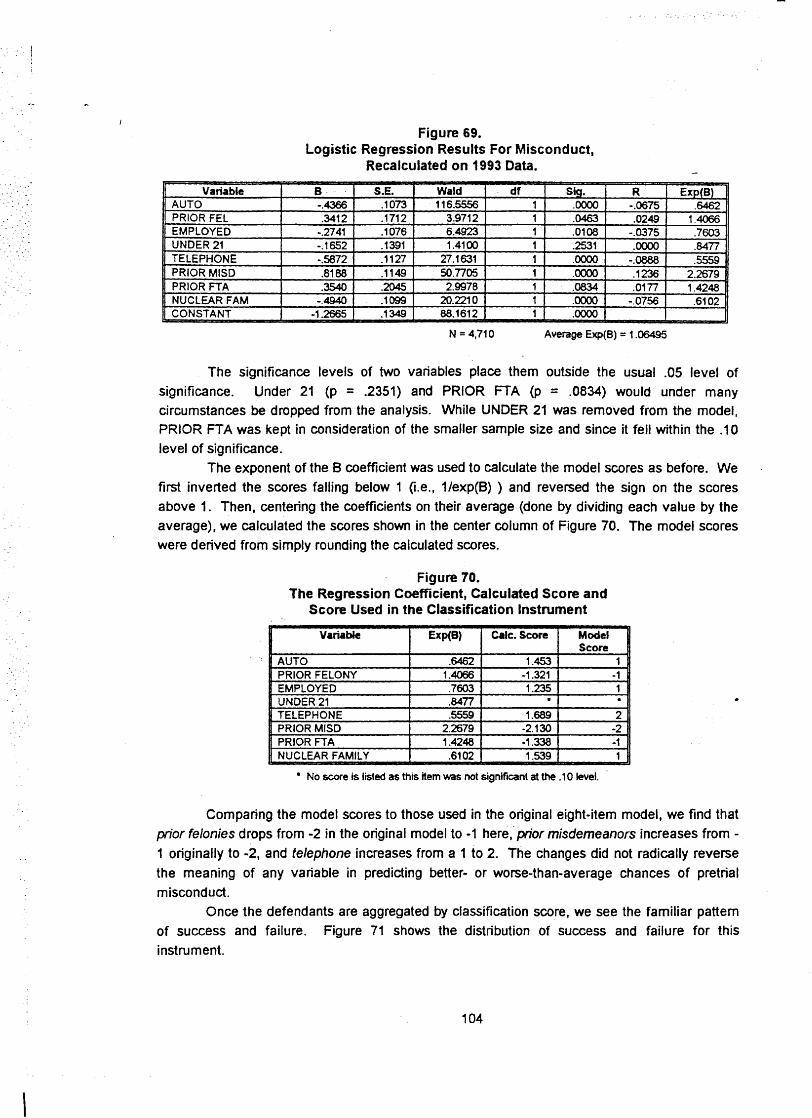
Figure 69. Logistic Regression Results For Misconduct,

Recalculated on 1993 Data.

The significance levels of two variables place them outside the usual .05 level of significance. Under 21 (p = .2351) and PRIOR FTA (p = .0834) would under many circumstances be dropped from the analysis. While UNDER 21 was removed from the model, PRIOR FTA was kept in consideration of the smaller sample size and since it fell within the .10 level of significance.

The exponent of the B coefficient was used to calculate the model scores as before. We first inverted the scores falling below 1 (i.e., l/exp(B) ) and reversed the sign on the scores above 1. Then, centering the coefficients on their average (done by dividing each value by the average), we calculated the scores shown in the center column of Figure 70. The model scores were derived from simply rounding the calculated scores.

Figure 70. The Regression Coefficient, Calculated Score and

Score Used in the Classification Instrument

1 Variabk I Exp(B) I Calc. Score 1 Model 1

H NUCLEAR FAMILY I .6102 1 1 539 1 1 l - - - - - - - -

No score is listed as this item was not significant at the .I 0 level.

Comparing the model scores to those used in the original eight-item model, we find that prior felonies drops from -2 in the original model to -1 here, pior misdemeanors increases from - 1 originally to -2, and telephone increases from a 1 to 2. The changes did not radically reverse the meaning of any variable in predicting better- or worse-than-average chances of pretrial misconduct.

Once the defendants are aggregated by classification score, we see the familiar pattern of success and failure. Figure 71 shows the distribution of success and failure for this instrument.

Distribution of Suc - - for t

I - Score 1 Success

Figure 71. :ess and Failure by Classification Score le Alternative lnstrument

Failure., I Total 1 %Fail I %Total (

While there appears to be a similarity to what has been found with the current instrument, a more careful examination of the results' of this reclassification must be made before conclusions may be reached.

The Results

Following the evaluation pattern, we see from Figure 72 that the mean cost rating for this alternative model indicates predictive power of 33.7 percent. Compared to the 30.2 percent of the original eight-item model, this represents a marginal improvement, at best. Allowing for shrinkage when applied to a sample other than the one on which it was constructed, it may be no better predictor than the current model.

Figure 72. Mean Cost Rating for the Alternative Instrument

Failure 1 Success ( P(Fail) 1 P(Succ) I C I U 1

Base Rate

Mean Cost Rating

Figures 73 and 74 show the significance test for improvement over the base rate. Clearly it is a significant improvement.

Figure 73. Classification Efficiency Analysis of the Alternative Model

1 I I I I I

! Total

Figure 74. ANOVA for the Alternative Model

II Source I Var I M I Std Error I F II

I Behveen

Within

The purpose of this analysis is in no way to suggest a change in the model. Rather, it is intended to demonstrate that some margin of improvement in predictive strength is likely (almost guaranteed) to be found if we attempt to optimize the model on each succeeding defendant cohort. The margin of return for so great an investment is likely to be low as that model is used on succeeding cohorts of defendants.

Nevertheless, there is likely to be a time when the decision environment spawns changes that require modification. It may be that existing elements need only be reweighted to account for the change; in other circumstances, whole items may be exchanged for new ones. It

0

is important to have the mechanism in place to recognize when significant change has occurred so that rapid evaluation and (potential) instrument reconstruction can take place in a timely

I Total

manner.

1 9.1 7876 430.229

449 .a78

Conclusions

Our stated goal in this project was to develop an instrument that characterized the collective experience of a jurisdiction-not one that dictates decisions. Taking this more passive alternative, we have left open the question of whether change is so endemic to the system that modeling the past provides no meaningful information for the future. We have found considerable stability in the characteristics that predict pretrial misconduct from the original study on 1990 data to the 1991 and 1993 validation studies.

4

4,716 4.794691 0.091 228

52.55751"

I

It seems very apparent that this classification instrument is a solid performer, providing consistent readings of the risk of one group of defendants relative to others. While the original study produced a model of reasonable but modest power, that power has not diminished over time. This retention of classification power has exceeded our expectations. -

We have further demonstrated that "fine tuning" the present model would not produce substantial improvement in predictive power (mean cost rating improvement of 3.5 percent). This demonstrates that the margin of return to be had may not-on an economic basis-justify the investment of time and resources required to change the instrument's implementation.

In sum, the instrument is operating as predicted. It provides a classification scheme that effectively disaggregates the defendant population into seven distinct groups, three falling on or below the misconduct base rate and four falling above. The inmates within these groups tend to behave collectively in a consistent and predictable manner. This significantly reduces the degree of uncertainty decisionmakers face when confronted with the question of personal bond release.

When properly applied as a decision support tool, this instrument could assist decisionmakers in reducing uncertainty concerning likely pretrial release outcomes. The instrument can remove about one-third of the total degree of uncertainty surrounding a pretrial release decision, thus enabling decisionmakers to become more focused upon the particulars of individual cases.

1

Section Nine The Impact of Classification

- . , ., - , - Minorities and Females . -

Introduction

With any policy decision there are both intended and unintended consequences. The line betkeen what is intended and unintended may become very fine when policy decisions are applied to the classification of defendants Pretrial classification intends to differentiate between groups of defendants with distinctly different failure rates, but there is no intention for these differentiations to cut along raciallethnic or gender distinctions. Whenever an instrument disproportionately distributes distinct groups of defendants (who ordinarily would have been grouped together) a k s s classification categories, questions concerning the legitimacy of the classification process may be raised. These challenges may be met only by empirically demonstrating that the categorization of defendants is independent of their racelethnicity and gender. This section presents our findings of the potential for disparate impact in the classification instrument.

The difference between information describing what the jurisdiction's experience has been and judgments defining what the jurisdiction's experience oughf to have been often is lost when assessing disparate impact. The difference between defining what oughf to be and the way things are, characterizes the difference between an application of objective and subjective classification methods. As we examine the impact of classification on minorities and females, we must keep the difference between subjective and objective classification in mind.

. .

Objective classification . .

. Objective classification is based upon the assumption that the instrument measures the 8 . .'

likelihood of failure that is independent of the decisions actually. made. In other words, the instrument purports to measure a quality inherent to the defendant in the absence of selection bias. The focus is therefore not on the actually observed proportion of defendants who fail from

* - one group or another; rather, it is on the proportion of defendants who would have failed if the

treatment of all indiyiduals were strictly identical. Objective classification is often used to develop normative inAruments that define how certain groups of defendants oughf to be treated.

. ~entencing~uidelines are an example of nonnative instrumentaion. . . A fundamental problem with this approach is that to neutralize the, effects of decisions

and produce conclusive results requires a controlled experiment with random assignment of cases to treatments. his is quite impossible in most areas of the criminal justice field, including pretrial release decisions. Quasi-experimental and non-experimental methods can apply elaborate statistical schemes to balance the effects of non-random assignment (Campbell and Stanley 1966)' but these do not yield results that unambiguously define underlying causal relationships and they may be challenged on the degree of objectivity that they actually achieve (Pedhazur, 1 982).

Subjective Classification

Criminal justice outcomes are the product of actions, reactions, the citizenry and of actors within the system; these outcomes are the network of decisions. Decisionmaking is a process of interpreting a

choices, and values of -

products of a complex set of conditions and

applying a system of values to choose a course of action from a set of alternatives, and past experience generally serves decisionmakers well in improving the quality of decisions made.

~ub jeb ive classification instruments summarize defendant and system interactions, reflecting the actual experience of the jurisdiction. We recognize these as subjective because decisionmaking exercises many subjective value judgments, making the outcome a subjective experience. If we build a classification instrument' on these experiences, it is a subjective classification instrument.

Applying a subjective instrument to a defendant population, then, does not dictate who should or should not be released. Rather, it indicates-on the basis of the past experiences of the jurisdiction-which persons are more or less likely to be declared a pretrial "failure." While supplying information that directly relates to the actual experience of a jurisdiction, it cannot determine whether these outcomes were the product of bias or equity since justice is based upon value systems and interpretations of events that extend beyond the scope of available data.

"Prohibited" Decision Criteria

A common practice is to ignore gender and racdethnicity as decision criteria in an attempt to promote equal treatment under the law. We agree that justice decisions should be based upon the merits of a case, and not- on the racdethnicity or gender of the defendant. However, we also would caution that ignoring prohibited criteria does not necessarily eliminate bias.

Many life experiences are strongly related to racdethnicity and gender, being a "single parent," for example, is highly associated with being "female" in our society. For the sake of illustration; let us ass"me that status as a "single parent" is a good indicator of low pretrial risk. We might be temptid to rationalize that added responsibilities, such as family ties, may be at the root (the cause of) pretrial success. But suppose low risk of failure is truly characteristic of *

females and not of single parents. Gender differences in this example are latent effects underlying the . "~ in~ le '~a ren t " . variable. v hat is, while %ingle parent" ma9 well be accepted as an appropriate criterion for decisionmaking, use of a person's gender as a criterion for pretrial decisions would draw criticism for applying a "prohibited" variable. The result is that single parent malesPmay be favored undesewedly in classification, while non-single-parent females are unfairly penalized. In this instance, including defendant gender as a variable in the classification analysis would have helped correctly identify the true source of variation and avert disparate treatment of defendants.

There are two lessons to be learned from this example. First, identification of persons by "prohibited" criteria does not have to constitute inappropriate discrimination if the information is to be used to understand decisionmaking and its outcomes and not to force decisions. Second, exclusion of these criteria does not eliminate the possibility of systematic bias through latent effects. Noting the irony, we would suggest that the justice system may be more

vulnerable to latent discrimination by purposefully excluding gender and race from decision analysis than if these were made part of the evaluation process (evaluation and decision processes being separate).

-

What Can be Learned from Disparate lmpact Studies? r .

We have stated that this classification study cannot unambiguously identify what should be done with a given group of defendants. Rather, the instrument identifies what the jurisdiction's past experience has been with defendant groups. It is therefore an encapsulation of past experience which decisionmakers may wish to consider in refining future decisions.

Condensing thousands of decisions into eight variables necessarily involves considerable aggregation. While aggregation achieves an unbiased overall measure when appropriate statistics are applied (as in the development of the present instrument), it may become biased when dividing the population into defendant groups not included in the original model. Because raceiethnicity and gender distinctions. were not included in the original data analysis, they may be subject to unintended bias in the way the instrument assigns risk.

Bias, in the context of this study, refers to the classification of certain types of persons in ways that place them at a disadvantage to other persons who repsent equal levels of risk. Bias could be said to exist if an instrument sysfematically classified females at higher risk levels than males if the observed rates of failure for females were equal to those of males. It would not reflect bias, however, if the instrument were to place more males in higher-risk groups than females if the failure rates for the males in those categories were similar to female rates in those categories. In sum,-an unbiased instrument provides equal classification for equal levels of risk.

We operationalize risk as the proportion of observed failures to the total released defendants. But this is not meant to imply that there is no bias in Rhe decisionmaking system itself. To ask whether appropriate release or revocation decisions were made calls for value judgments that must be resolved in a political arena where our system of collective values is negotiated. To ask whether the instrument accurately portrays the level of risk as experienced in Hanis County, however, is an empirical question that we can address here.

Examining the Classification Instrument for Disparate Impact

This examination consists of dividing the defendant population into raciallethnic groups, separating males and females, and then aggregating the misconduct rates for each group according to their classification scores. Applying tests of proportions between groups, such as male and female, for each level will yield an assessment of whether a significant difference exists.

The data from 1991 and 1993 were both tested, as each had strengths for this analysis. The 1991 data offer greater numbers of cases, thus providing greater statistical power. Statistical power measures the likelihood of correctly identifying relationships that truly exist. The 1993 data, while only covering the first quarter of the year, offer a measure of actual field performance.

Presenting results from both 1991 and 1993 also serves another purpose. The failure rates observed for any category in any given year is subject to random fluctuation. Whenever we present findings from a single sample, however, there is a tendency to view them as fixed

I

values, leaving readers with the assumption that this pattern will remain the same over time. By reviewing the results of two samples, the reader may better appreciate the degree to which observed rates may vary by category over time. The point we hope to make is that whether the results favor a desirable outcome or not, scientific principles require multiple and periodic tests - of instrument performance to assure that the findings reflect the "true" pe;formance characteristics of the instrument.

Comparing Females to Males

The first question we address is whether males and females are equitably classified by the instrument. The findings for both 1991 and 1993 are presented at each step to facilitate comparison.

From Figure 75, we can see that males generally had a slightly greater likelihood of failure than females (1 1.79 percent and 13.82 percent, respectively) in the 1991 sample. Females range from a low of 5.85 percent failure for classification level 4, to a high of 51.72 percent in category 4. Males range from 5.94 percent failure for classification level 4 to a high of 42.67 percent for the <-1 category. For both males and females, there is a monotonic increase in the failure rate from category 4 to 4.

Figure 75. Distribution of Female and Male Pretrial Release Outcomes by

Classification Level for the 1991 Sample

I Females I Males 11

The 1993 sample reflects considerably lower overall failure rates, 9.15 percent and 9.71 percent for females and males, respectively. The scores for females range from a low of 1.46 percent failure among those classified in category 4, to a high of 22.22 percent in category 4. Males show a 4.01 percent failure in category 4 with a high of 21.54 percent in category <-I. As in 1991, the change in failure rates follow a monotonic increase as classification scores decrease.

Figure 76. Distribution of Female and Male Pretrial Release Outcomes by

Classification Level for the 1993 Sample

In the 1993 sample, males appear to have greater failure rates than females in the lower-risk categories (0 to 4), whereas females seem to have greater failure rates than males in the high-risk categories (-1, 4 ) . To establish whether this observation is likely due to random differences or constitutes a systematic pattern, we turn to a test of proportions. Figure 77 shows the results of these tests for each classification level.

There are three classification scores in which males evince significantly higher scores than females (t-values shown in bold face). Two of these (0, and 1) are barely significant, both scoring a -2.09 when a i1.96 was required for a significant finding. This indicates that in 1991, the instrument would have grouped some femalbs and males with different rates of failure. For the 0 category, the difference would have been 4.65 percent, for the 1 category, 3.75 percent and for category 3, 3.98 percent. Other differences, such as for the c-1 group, appear larger than those identified, but this difference is weakened by the small number of cases, making these differences reasonably attributable to chance.

Figure 77. Comparison of Male and Female Pretrial Misconduct Rates and Numbers with Total Released by Classification Score

for the 1991 Sample

'A t-value of f 1.96 or greater is required for significance.

Class. Scwe

<-I

-1

0

In contrast to 1991 findings, the actual failure rates observed for the 1993 defendants shows no significant differences between male and female defendants. Figure 78 shows no t- value that is significant for any of the seven risk categories. Only classification scores 0 through

Female

51 -72%

27.1 4%

15.06%

Male

42.67%

26.32%

19.72%

Difference

9.06%

0.83%

-4.65%

Std. En.

0.1 00726

0.057148

0.022236

t-value'

0.89921 7

0.144725

-2.092280

I

3 contain enough female defendants to yield valid test results. Among these, the greatest difference (1.41 percent) was found between females and males in the 0 category.74 This difference could be erased with 2 additional female failures, and is clearly a difference that could be driven by chance, as the non-significant t-valueindicates. - -

Figure 78. Comparison of Male and Female Pretrial Misconduct Rates and Numbers with Total Released by Classification Score

for the 1993 Sample P

Std. En. 2-value*

'A t-value o f f 1.96 or greater k required for significance.

Figure 79 graphically illustrates the comparison of the 1991 failure rates for females and males for each classification score by the range predicted from the 1990 data. The confidence interval represents the range of values the failure rate may take on as a result of random fluctuation over time. Any score falling within its confidence interval is said to be similar; those falling outside the interval are said to be (significantly) different. Figure 80 shows that most of the 1993 observations fell within or above their expected ranges. This casts the 1991 data into a new light. Whereas in Section Seven we demonstrated that the 1990 and 1991 data sets overlay each other well once the base rates have been adjusted to compensate for the greater number of pretrial failures in 1991, the group failure rates for females and males suggest that the differences may be more due to an increase in male failures than female.

--

7 4 ~ h e bhriate approximation of a normal distribution requires a minimum of 10 observations in the smaller category, in this

case, pretrial failures.

Figure 79. Comparison of 1990 Confidence Intervals, Female and Male Failure Rates by

Classification Score for the 1991 Sample

Failure R.t.

0.5 - Confidence Interval

-8- Female

t I -f3 Male

0 0.1 0 2 0 3 0.4 0.5 0.6 0.7 0.8 0.0

Proportion d th. Population

The 1993 data, when arrayed against the 1990 confidence intervals, shows very good consistency with the confidence intervals. The female and male rates of failure fall within the confidence interval defined from the 1990 data.



0.45 t 1 - Confidence Interval

O,' t I + Female

-f3 Male

0 0.1 0.2 0.3 0.4 0.5 0.6 0.7 0.8 0.0

Prowrtion d the Po~ul6tion

The tests reported here seem to lead to conflicting conclusions. The test of proportions show significant differences for 1991, but not for 1993. The comparison to confidence intervals seems to suggest the variation is largely within expected limits established on 1990 data. Given



Failure R.t.

0.5 8 ' " Confidence Interval

-) Female

t I -R- Male

0 0.1 0 2 0 3 0.4 0.5 0 6 0.7 0.8 0.0

Proportion d the Population

The 1993 data, when arrayed against the 1990 confidence intervals, shows very good consistency with the confidence intervals. The female and male rates of failure fall within the confidence interval defined from the 1990 data.



0.45 t 1 confidence lntenral

0.4 t I -W- Female

-R- Male

The tests reported here seem to lead to conflicting conclusions. The test of proportions show significant differences for 1991, but not for 1993. The comparison to confidence intervals seems to suggest the variation is largely within expected limits established on 1990 data. Given

*

, the large number of cases that were compiled to produce the failure rates, these findings of significant differences between males and females in 1991 cannot be ignored, but also we must hold open the possibility that the failure rates are subject to fluctuation and may be showing more or less extreme variation. -

But 1991 is only a projection of potential impact; the 1993 data, though containing fewer cases, represents actual application. By examining the 1993 data separately, we begin to see the formation of a different picture. While insufficient data exists to draw conclusions about the significance of misconduct rate differences between all classification levels of male and female defendants, a test of proportions (following the formula shown on page 88) indicates that no significant differences have yet emerged. If the findings shown in Figure 80 hold for all of 1993, the model could be judged as giving very consistent treatment to both males and females.

Comparing Major RaciaVEthnic Groups

As we have stated previously, the Hams County justice system differentiates its population into four raciallethnic categories: African-American, Hispanic, Anglo, and Other. Of these, the first three groups represent the majority of the defendants. While defendants of the "Other" category are no less important than their counterparts in the other groups, their numbers within the sample are too small to generate reliable estimates within any classification category and we have therefore elected to compare the three primary raciallethnic groups. Figure 81 shows the distribution of Hispanic, African-American, and Angio defendants and their observed misconduct rate by classification score for 1991, and Figure 82 reflects similar distributions for

Figure 81. Comparison of c is panic, African-American, and Anglo Pretrial

Misconduct Cases and Number Released by Classification Score for the 1991 Sample

Class. Misc. Score Cases

c- 1 5

-1 7

0 46

1 53

- --

isp panic I Black

Total 1 Misc I Misc. I Total Misc Rate 50.00%

28.46%

20.25%

Cases Rate Cases Cases 19 26.32% 49 98

2 82

3 58

4 23

Total 274

Figure 82. Comparison of Hispanic, African-American, and Anglo Pretrial

Misconduct Cases and Number Released by Classification Score for the 1993 Sample -

S z y 1 Cases

Total I 130

Hispanic Black White

Total I Misc Misc. 1 Total I Misc Misc. I Total I Misc Cases Rate Cases Cases Rate Cases Cases Rate

10 20.00% 11 34 32.35% 3 14 21.439

The overall misconduct rates for 1991 were lowest for Hispanic defendants (1 1.21

percent) and highest for African-Americans (16.60 percent), for a difference of 4.33 percent. By contrast, the 1993 data show the difference between Hispanic and African-Americans to be 2.4 percent, based upon a 9.77 percent and 12.17 percent rate, respectively. To address the question of whether the instrument is misclassifying defendants belonging to any given raciallethnic group, we must apply a test of proportions to these data. Using Anglo defendants as the basis for comparison, Figures 83 and 84 compare Hispanic and African-American defendants to Anglo defendants by classification score.

Figure 83. Comparison of the Failure Rates of Hispanic and Anglo Defendants by

'

Classification Category, for the 1991 Sample

1 Class ( Hispanic Failure 1 Anglo Scores Rates Failure Rates

<-I 26.32% 40.98%

Figure 84. Comparison of the Failure Rates of Hispanic and Anglo Defendants by

Classification Category, for the 1993 Sample -

Figure 83 shows that only in category 1 do Hispanic and Anglo defendants vary significantly in rates of failure for 1991. The t-values for <-I and -1 are not shown because there were insufficient numbers of cases to validly test the differences in proportions. The 1993 data show no significant difference between Hispanic and Anglo defendants. ~ i ~ u r e 84 shows three blank t-value categories, indicating that there were three groups that had insufficient numbers for valid tests of proportions.

Comparing African-American with Anglo defendants (Figure 85), we find that only in category 3 is there a significant difference. There, we see that African-Americans experienced 2.69 percent more failures than Anglos belonging to the same risk category. Even though the differences in failure rates are larger in categories <-I and -1 (where Anglo failure rates are 5.55 percent higher), the small number of defendants that make up these categories weakens the difference within the statistical analysis to a degree that falls below 95 percent confidence that these are not due to chance. By contrast, in 1993 only categooy-1 _Showssignificant differences,

- - - - - - - - - - - - -

meaning that i t i s the ~ngloaefendants who have a higher failure rate than their African- American counterparts (Figure 86).

Figure 85. Comparison of the Failure Rates of African-American and Anglo Defendants by

Classification Category, for the 1991 Sample a

I .-. - .-. . * . r . - I . t . > . .".. . . . . , - . .. ,.,. ., , . : Figure 86. .,.

~ompar i id i i of the ~ & l u i e pate= of African+neric& &d Anglo Defendants by

- , . . v u I 6 . > - . ,.- ' 3 . r ~lassificatibn Category, for the 1993 sample

, - . .

Based upon the foregoing comparisons, differences between Hispanic and Anglo defendant classification and differences between African-American and- Anglo defendant classification would have no impact on release decisions if the scores of 2,3 and 4 were treated as a "low risk" group, scores of 0 and 1 were considered "medium risk" and scores of <-I and -1 were considered "high risk." - .

Figure 87.--- ' . Comparison of 1990 Confidence Intervals, Afkan-~merican,'~ispanic. and-Anglo Failure Rates by Classification Score for the 1991 sample

. . . r

. .-.. or is-

,< - .. . . . = . . . . . - .- . + African-American

.,.:> 2 :: , : ,, . : .,, ' . . . . --

q I ; ,C[~! .? , - . , : . . -.. .,. . .~ - % . - . . ' L.8 '

- , 9 ' Hispanic ' ; ,

. .

. . - . :. 0.05 -- . .

. . . . . . . . . . . . . . . . . . . . . , - . . . .. - .

0 0.1 0.2 03 0.4 05 : 0.6 . 0.7 ' 0.8 0.D . .

~ d t h e f o w ~

a , r Z

The relationships between the& threeq groups can be pla&d 'in perspective by comparing their obsbhed Gtes of failure with the'predicted rates of failure from 1990. ~igui;! 87 illustrates these &lationship;.- - With-the dark bars ;epresenting expected ranges of variation

' (confidence iniervals) based upon the 1990 data, the smaller squares mark the obsehed failure rates of the three groups within each of the classification levels. Ideally, the squares should fall inside th& krkdence interval for each level. With the 1991 data's high overall failure rate, there is a general "pwaid dispI'$&ment ofdbserved failures relative to the 1990 confidence intervals.

r . * - A \ I \ -

1

A visual scan suggests that if the confidence intervals from the 1990 data were adjusted upward to account for the change in the 1991 failure rate, the distribution of Hispanic, African-American, and Anglo defendants would approximately fit within the confidence intervals.

The 1993 data likewise shows close conformity with the 1990 confidence intervals, - suggesting a consistent treatment by racelethnicity. Figure 88 demonstrates this graphically.

-

Figure 88. Comparison of 1990 Confidence Intervals, African-American, Hispanic,

and Anglo Failure Rates by Classification Score for the 1993 Sample

0.45 1 1 I Confidence Interval

+ African-American

+ Hispanic

%- Anglo

As with the comparison between females and males earlier in this section, the patterns observed here are not written in stone. The failure rates by classification level and by defendant group will vary over time. While the 1993 data cannot be used for conclusive statistical analysis due to the paucity of cases at many classification levels, we can see different patterns forming than were observed above (see Figure 14). The 1993 data show considerable convergence in the misconduct rates of the three groups with generally diminishing differences between them across the classification levels. This is consistent with the findings for males and females and suggests that the instrument should function without excessive bias over time. -- .:.

Testing for Combinations, of Effects

Recent trends in the research literature suggest that racdethnicity and gender should not be examined independently. System responses to persons may differ, depending upon the combination of raciallethnic and gender combinations. Being African-American and male may elicit a different reaction than being either Anglo and male or African-American and female. These combinations, called interactions in statistical terms, may be tested to see if these ..- 1

combinations impact outcomes. A logistic regression model was c o n s t ~ ~ t e d to determine whether an interactive effect

between racelethnicity and gender could be found that, would add to our understanding of the L - - .

distribution of misconduct among the seven classification levels. Table 89 summarizes the best-

I

fitting model derived from that analysis for 1991. This table shows that for each step in classification score (called "Class" in the variables column), the failure rate is .7339 (73 percent) of the former category (shown in the "Exp(B)" column). African-Americans average about 16 percent higher rates of failure than Anglos, while Hispanics fail at about 85.75 percent the rate of - Anglos. Females fail at 81.05 percent of the male rate and there is no significant interaction by gender over classification levels.

Table 89. Summary of the Best Fitting Logistic Regression Model Using RaceiEthnicity and Gender for the 1991 Sample

I

Fern ' Class 4.0429 0.0478 0.8055

'Constant -1.2909 0.0489 703.6%

By contrast, the 1993 data show only a significant difference attributable to classification score. No racdethnic or gender variable or interaction was significant. This justifies the independent treatment of racdethnicity and gender.

Table 90. Summary of the Best Fitting Logistic Regression Model Using RaceEthnicity and Gender for the 1993 Sample

1 I I I I I I

Constant 1 -1 -46251 0.1 0071 21 0.94551 1 I 0.oo0ol 1 11 - - - - - - - -

e

his table (Figure 90) shows that the difference between females and males (B=.266, Sig = .0940) is not significant. This means that we cannot be sure, based upon- these observations, that women are failing at clearly lower rates than men with the same classification score. ~ i s ~ a n i c is also not significant, suggesting the difference in failure rates observed between Hispanic and Anglo defendants is not outside the range of random chance. The Af-Am variable shows significance, indicating that as a group they experience pretrial failure at significantly higher levels than Anglo defendants. Finally, the Fern Class interaction term shows significance, indicating that female failure rates differ significantly from those for males, but whether it is higher or lower depends upon the classification level. We found female defendants typically exhibited fewer failures in the low-risk groups, while they had higher rates of failure than males-in the high-risk groups.

As we examine these findings, it should be kept in mind that even with 116 percent difference in failures between African-American and Anglo defendants, the rates are attenuated

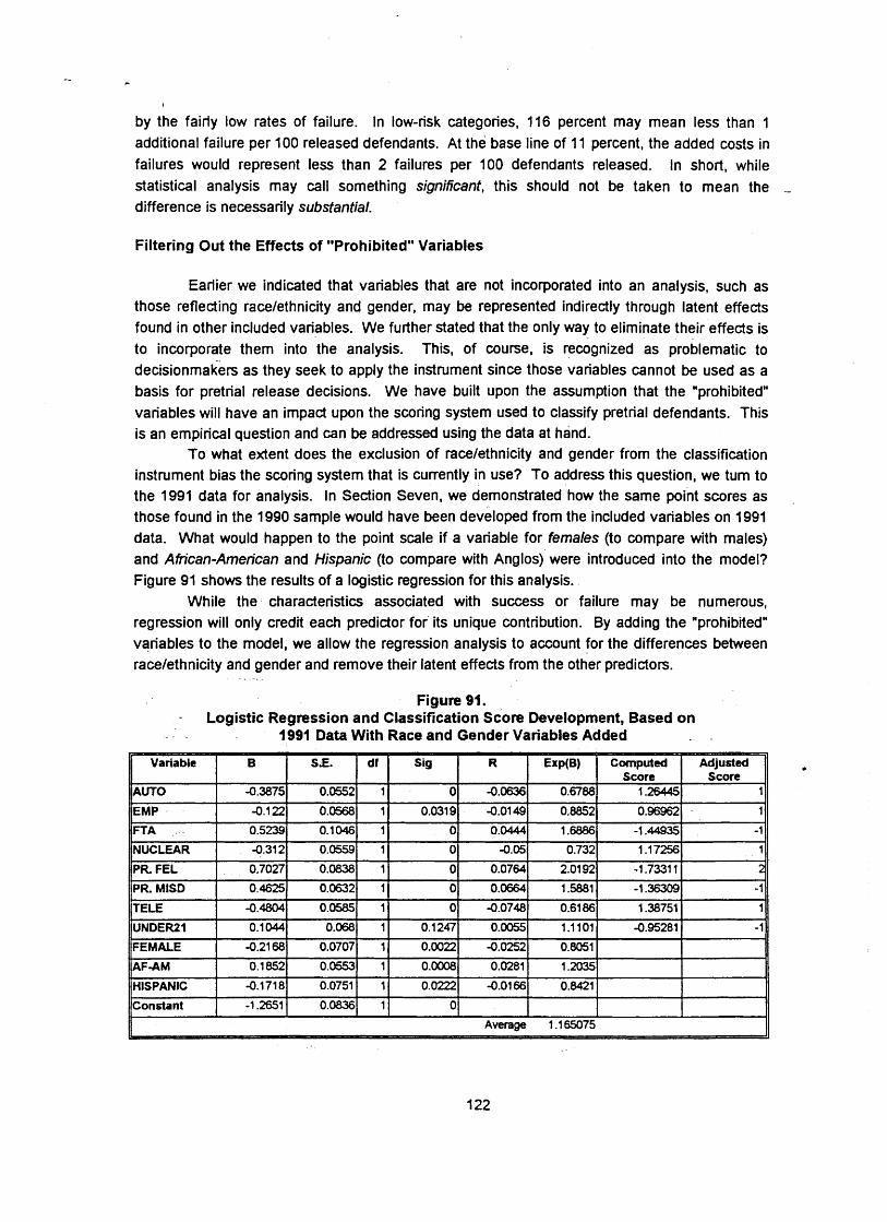
I

by the fairly low rates of failure. In low-risk categories, 116 percent may mean less than 1 additional failure per 100 released defendants. At the base line of 11 percent, the added costs in failures would represent less than 2 failures per 100 defendants released. In short, while statistical analysis may call something significant, this should not be taken to mean the -

difference is necessarily substantial.

Filtering Out the Effects of "Prohibited" Variables

Earlier we indicated that variables that are not incorporated into an analysis, such as those reflecting racelethnicity and gender, may be represented indirectly through latent effects found in other included variables. We further stated that the only way to eliminate their effects is to incorporate them into the analysis. This, of course, is recognized as problematic to decisionmakers as they seek to apply the instrument since those variables cannot be used as a basis for pretrial release decisions. We have built upon the assumption that the "prohibited" variables will have an impact upon the scoring system used to classify pretrial defendants. This is an empirical question and can be addressed using the data at hand.

To what extent does the exclusion of racelethnicity and gender from the classification instrument bias the scoring system that is currently in use? To address this question, we tum to the 1991 data for analysis. In Section Seven, we demonstrated how the same point scores as those found in the 1990 sample would have been developed from the included variables on 1991 data. What would happen to the point scale if a variable for females (to compare with males) and African-American and Hispanic (to compare with Anglos) were introduced into the model? Figure 91 shows the results of a logistic regression for this analysis.

While the characteristics associated with success or failure may be numerous, regression will only credit each predictor for its unique contribution. By adding the "prohibited" variables to the model, we allow the regression analysis to account for the differences between racelethnicity and gender and remove their latent effects from the other predictors.

Figure 91. - Logistic Regression and Classification Score Development, Based on

- - 1991 Data With Race and Gender Variables Added - -

I Variable I I I

EMP - 0 . 1 0.0568

FTA . 0.5239 0.1046

NUCLEAR -0.31 2 0.0559

P R FEL I 0.7027 0.0838

P R MlSD 0.46'25 0.0632

T E E -0.4804 0.0585

UNDER21 0.1 044 0.068

FEMALE -0.21 68 0.0707

AF-AM 0.1 852 0.0553

HISPANIC -0.1718 0.0751

Constant -1 . a 1 0.0836

df Sig R Exp(B) Computed Score

1 0 -0.0636 0.6788 1 26445

Adjusted Score

1

Average 1 .I65075 II

I

Figure 91 represents the variables that are presently being used in the Hanis County classification model, with three variables added. FEMALE represents the difference in failure rates between males and females; AF-AM (African-American) and HISPANIC represent the difference in failure rates in those two groups relative to Anglos. With the inclusion of the three - "prohibited" variables, UNDER21 falls below the significance level of .05. We have included it in the analysis, however, to compare the scores developed from the original data set and this one.

Now that we have statistically removed the effects of prohibited variables from the other predictors, we can create a point scale in which the point scores are free from their influence. If we exclude the prohibited variables from the point scale we can affirm that the scale has been "cleaned" of any direct influence due to racelethnicity or gender. This process produces a suboptimal model from a statistical point of view, but it represents one that is practical given procedural constraints.

The Computed Score column shows the scores resulting from the method of calibration used in previous sections. First, we take the average of the exponentiated coefficients (U(P(B) column), in this case excluding the effects of the "prohibited" variables, and divide each of the Exp(6) scores that are 1 or more and changing their sign from positive to negative. For those falling below 1, the scores are inverted (divided into 1) and then divided by the average . The results, shown in the Computed Score column, are then rounded to integer values. These are shown in the Adjusted Score column. Compared to the original point scale, they were found to be identical.

This means that the model in its present form is performing in as unbiased a form as if racelethnicity and gender had been statistically controlled. This suggests that either the observations showing significant differences for certain categories are an artifact of random variation, or the relative mdi ty of the instrument is not allowing more refined assessments of pretrial risk. In the opening section, we discussed what was necessary for a pretrial risk instrument, and simplicitywas a high priority. As long as people have to calculate a risk score in their head, there will be a need for an simplified method of classification. We may find, however, that "rounding the cornersa on our assessments of risk may actually desensitize the instrument from picking up nuances that may be present in the computed scores.

These findings support the performance of the present model, demonstrating that the differences in treatment between the groups would have been the same even if the special status of each group had been taken into account. On the weight of present information we feel this model is performing well. Time and repeated trials will be necessary to positively identify the presence or absence of bias.

Conclusions

If our sole interest were to "sell" the classification instrument to Hams County, we would have presented only the 1993 findings of disparate impact. Those findings would have painted a rosy picture of minimal disparity which, while perhaps convincing, would foster the assumption that the favorable outcomes would be consistently observed over time. It is important to understand that the findings will vary from one sample to another. The underlying pattern is sufficiently consistent that the instrument seems to work reliably over time, but the exact results will be subject to variation.

While the classification instrument has been shown to work with reasonable reliability across two validation samples, we find that there are some discrepancies in the way that some defendant groups are classified. These discrepancies, while statistically significant, do not represent excessive differences nor do those differences appear to persist over time. What has -

appeared to be significant differences in the projected impact analysis (1991 data) seems to be diminishing in actual experience with the 1993 data, showing considerably smaller differences between groups.

But even if differences persist, they may not actually result in different treatment. If the classification scores are grouped according to bmad risk levels (4,3, and 2 representing low risk, 1 and 0 representing medium risk, and -1 and <-I representing high risk), the differences between most groups disappear. Only differences that exist at a break point will bear any potential for differential treatment.

Bias represents the unequal treatment of equivalents. When defendant groups are not evenly distributed across all levels of a variable, any attempt to use that variable to classify defendants can result in bias if the uneven distribution'is not controlled. Most variables are disproportionately associated with racelethnicity or gender. Offense type, social, and economic variables all posses a degree of disproportionality with respect to the "prohibited" variables. This makes them vulnerable to statistical bias.

The type of bias more likely to be sought out is related to the fair treatment of defendants by the system. "Fairness" and other terms related to justice issues are moted in our values systems and philosophy. Much of what goes into values falls outside of the JlMS system and our ability to capture and analyze data. We can report the Harris County experience as succinctly as possible in the form of a classification instrument, relegating the concerns for justice to the political sphere where such issues can be more effectively addressed.

These constraints notwithstanding, we have demonstrated that this classification model is identical to one in which the impact of racelethnicity and gender has been controlled. This suggests that the present set of predictors are functioning without direct bias against racelethnicity or gender. Deviations in failure rates between groups at certain risk levels may be due to random variation, or due to the crudity of the additive points scale approach to classification. By reducing coefficients to integer values to aid score computation, we may be blunting the instrument's ability to make fine distinctions. If either of these possibilities are responsible for the observed differences, they should not remain the same over time; subsequent analyses should show new patterns (though not radically different) between defendant groups. We see this happening with the patterns formed in the 1993 data.

Disparate impact and its effects must not be taken lightly. But neither should there be an overreaction to a single set of findings. The failure rates of groups, however defined, tend to vary from one time to another within set limits. Any observed relationship between groups may not be consistently observed over time but as the limits of their variation becomes better understood a high degree of predictability develops. Further, 1991 reflects projected impact of the classification instrument, not observed. Actual 1993 experience do not appear to support our projected findings. More data on theactual use of the instrument will help clarify these issues.

These findings suggest continued observations are important. Whether the instrument is or is not performing to personal satisfaction, the need to reevaluate it periodically is equally important. Changes in the decision environment can lead to changes in the instrument's

I

performance which in turn may require modifications if the instrument is to continue to perform a useful role in bail classification.

Introduction

Section Ten Classification Information for Strategic Planning

1 1, I

+. - , - : ; . , .

, .

In the preceding sections we have shown how JlMS data may be used in classification research. We have also shown how the dla&ification instument may be used to better understand the underlying relationship between certain criteria and failure rates. Classification research, however, can produce a number of benefits besides creating and validating a classification instrument. The data may be used to develop an understanding of present circumstances and to seek altematives for more effective resoup management.

What are the costs and consequences of current practices? It is important to develop a base line for comparing altematives. One cannot know if a change will be beneficial unless the

I

anticipated results can be compared to present experience. -Often by simply presenting a model of current practice, decisionmakers can readily assess whether expected objectives and goals are being reached.

What is the expected impact of alternative policies on the present circumstaks? If a policy change is considered desirable, proponents must pursuade others of their point of view before a policy can be implemented. The difficulty of this task is to some degree related to the clarity with which the problem and proposed solution can be expressed. Providing data directly from the experience of the jurisdiction is a definite advantage in facilitating positive change. - - c his section explores two applications of the present research to policy issues to illustrate how it may be applied to any number of questions. - - he first example examines the impact . , of .. present practices on non-released defendants who later serve a community-based

.a -i

.sentence. The'second e iam~ le estimates thebbtential im~act of an iniiati"e to extend ~ersonal bonds to a lame number of defendants. -

The Disposition of Non Released Pretrial Defendants ' "*"- -

,\1 - An example of how classification research can assist in evaluating current practices can .

be found in examining the number and dispostions of non-released pretrial defendants. Persons detained because they cannot make bail consume jail bed resources until their case is disposed. Some suggest that holding a defendant in jail during the pretrial stage, then sentencing the defendant to probation or another community program is a waste of resources. If once convicted, the offender is deemed "safe" enough retum to the community, what rationale would justify the pretrial detention of that same individual?. : t-

i To be sure, there are legal constraints on sentencing in some cases in which "dangerous" offenders must be incarcerated on the basis of the crime of conviction. Many persons may represent an unknown risk to the community or a potential for nonappearance in court. Other cases may simply "fall through the cracks" in the system, where good risks are held because they are unable to make bond and for whatever reason are not offered a personal bond.

How many remain in jail until disposition of their case? Of the defendants in our 1991 sample, 13,049 defendants did not receive pretrial release.. Figure 92 shows the distribution of the non-released defendants by classification scores and type of disposition. Of those, 10,387

persons failing for each classification score including all classification scores of lesser risk (the failures presented below a given class score in the figure). These cases are divided by all those released (all cases presented below a given class score in the figure).- The resulting rate is the proportion failing, shown in the final column. By consulting this column, we see that those falling - in categories 1 through 4, if released, would maintain the approximate rate of failure observed in the released cases.

Figure 94. Expected Failure Rates for Alternative Release Policies

C1assifi;tion Lydui: Score

Expect Number I Cumulative Misconduct Misconduct

87.1 84 675.452

Cum. Proportion Misconduct

0.1 541

If the beds occupied by defendants scoring a 1 through 4 on the classification instrument .

were released shortly after pretrial interview, the net savings in jail space would be a function of the number released who otherwise would not have been released (the "No Bond" cases) and the number of days they spend in jail until their case is completed. Figure 95 shows the number of "Not Bonded" cases by classification score, their average time to disposition, and the number of bed-days saved. A bed-day is the number of beds occupied by defendants summed across the number of days they spend in jail; one physical bed, therefore, represents 365.25 bed-days when spread across the course of a year.

Figure 95. Expected Jail Bed Savings if all Classification Scores

from 1 to 4 Were Released

1 Classification I Not 1 Average Days 1 Bed Days I Annualized 1 Score

When the beddays saved represents the average number of days from pretrial interview to disposition, multiplied by the number of defendants not bonded, these bed days represent the savings attributable to the first quarter of 1993. Extrapolating to the full year, we might expect

Bonded 1,097

1 I

that 4 times that number would be saved over the course of the year. Since each physical bed

- 2

3

4

Total

I J

represents 365.25 bed days, we need to divide the number of (annualized) bed-days by 365.25,

to Disposition 15.61 35

10,406.990

4.1 88 .996

1,066.000

32,789.990

yielding the annualized savings in beds, shown in the right hand column. In total, 359 beds potentially could be freed by implementing this policy.

1 13.971 1

45.8754

1 1 -6742

359.0964

865

405

1 25

2,492

Saved 17.1 28.01 0

12.031 2

10.3432

8.5280

Savings 1 87.5757,

I

From the figure, one will note that the most substantial savings comes from those groups that represent the greater risks. By adding classification level 1, the number of freed beds more than doubled (adding 187 beds) at the cost of an additional 2 percent in the misconduct rate (representing 139 failures). This underscores a common finding in criminal justice: that the - altematives that yield the greatest benefit in one area usually come with the greatest costs in other areas. Balancing the savings in jail beds must be weighed against the cost of added misconduct.

No policy should dictate strict adherence to a classification instrument. While the present instrument has demonstrated accuracy in classifying risk, it should serve only as a starting point for the decisionmaking process. The instnrment is not intended to incorporate the details and the "intangibles" that weigh in the balance within a system of individualized justice. As such, decisions should reflect individual circumstances with respect to the broader system- wide experiences which are codified within the classification instrument.

Conclusions

The costs and complexity of justice in modem society requires that policy should be founded on sound reasoning and tangible "facts." An empirically-validated classification model can be useful not only in reducing uncertainty regarding outcomes for individual defendants, but also in assisting policy development by providing measures of risk on which present policy may be compared to altematives, or against which altemative policies be "bench tested" before undergoing the financial and political costs of implementation.

This chapter has demonstrated through two examples how current practices could be assessed or altemative policies be evaluated. Even though the two questions address different aspects, the classification instnrment proved to be a source of information for both. If pretrial release opportunities were offered to defendants classified as low risk by the instrument, cosiderably fewer community-sentenced defendants would remain in jail, the rate of failure on pretrial release would not change substantially, and 300 or more beds potentially could be vacated in the county jail.

We realize that many other considerations (i.e., political, fiscal, and legal) must be added to the formulation of policy. Analysis based upon the classification instrument provides a valuable source of information to support decisionmaking by reducing uncertainty; it cannot and should not dictate a solution.

Section Eleven Summary and Conclusions

Introduction

Since the dawn of prehistory, humans have used tools to raise their potential beyond the limits of the human frame. Today, the complex machinery of the information age has vastly broadened our potential to learn beyond the range of direct experience. We view events in our homes as they occur around the worid and we evaluate detailed data of routine activities that give us a perspective that transcends the limits of direct experience. Computer scientists are now developing methods of knowledge discovery that will not require direct human involvement.

This project is an example of how information can be used to extend our knowledge beyond the limits of individual experience. The bail classification instrument developed here represents the collective experience of the Harris County courts. The instrument codifies this information in as few items as possible, so that the benefit of this experience may be generalized to as many future cases as possible. By achieving considerable breadth of coverage, there is a loss of individual-level detail, thus the need to integrate classification information into a decision process involving other informational sources.

In the broadest terms, this project provides Hams County with a decision support framework for bail decisionmaking. We use the term "framework" in recognition that this study offers a change in the way we think of data and the uses to which they may be put. This framework: (1) enables decisionmakers to estimate the degree of risk involved in the release of a defendant, (2) enables policymakers to balance the competing concerns of public safety, public opinion, court mandates, cost effective administration of resources, and justice; and (3) establish and maintain an on-going, automated process to assure that a quality, low-cost decision support tool is maintained.

Findings

The primary purpose of the Hams County Bail Classification Profile Project was to evaluate the existing classification instrument and improve upon it, if possible. To that end, we presented four models for bail classification. We provided measures of the existing model's classification efficiency (mean cost rating = .1635), which showed that (1) the former model in its standard form did not differentiate well between most of the groups of pretrial defendants on their likelihood of pretrial miscondukt, (2) there was considerable disordinality in the failure rates of defendants at many failure levels (scores of 0 are better risks that scores of S), and (3) it could be substantially improved by removing two items and reweighting the rest of the items. The cost of implementing the reweighted model, such as reprinting forms, retraining staff, and changing automated information screens showed no inherent benefit over totally reworking the items. A search for better predictors was undertaken, which resulted in three potential models.

The five-item model was the smallest of the three models. Its strengths included maximum predictive power with a minimum number of items, and most of the items were already used by PTSA. The nine-item model, with more items contributing to the predicted score, generated more risk groups. That would have enabled finer distinctions between groups

I

and would have provided policymakers with more alternatives on how to divide the population. The nine-item model did not improve on the predictive power of the five-item model, despite being almost double in size. As well, the nine-item model included a single offense variable (trespassing) which appeared to be a statistical artifact. With the deletion of the offense -

variable, the model's items were reduced to eight, while its predictive power remained on a par with that of the five-item model.

Comparing Alternative Models

Which of the remaining models is the best? Perhaps the appropriate way to compare them is by their ability to increase the numbers of defendants eligible for release on personal bond without presenting a substantially higher level of risk to the community. We know from our earlier discussions that the average failure rate for the study defendants was approximately 11 .I percent, and we have seen the failure rates for individual groups within each model. But we must also consider the average rate of failure to be expected from two or more groups com bined-the pooled failure rate @fi)

The following figures provide us with several pieces of information, reading from left to right: (a) the group scores, in which higher numbers indicate better risks; (b) the proportion of the defendants belonging to each group; (c) the cumulative proportion (reading from the bottom up); (d) the failure rates for each group; (e) the group proportion multiplied by the group failure weight to remove any weighting effects; and (f) the pooled failure rate. This rate indicates the expected level of pretrial misconduct at each level of the three models. It is important to note that the pfr, as shown, has a degree of variation and the figures may be conservative.

In the reweighted model (Figure go), for example, we could expect a pfrof 9 percent with the release of defendants belonging to groups which scored a zero or higher. In actuality, we could approximate the known failure rate of .I 11 by selecting defendants scoring from a 2 to a -2 (1 1.2 percent pfr), and recommend 72.8 percent of the defendants as eligible. The reweighted model, however, refleds a lack of order in the group failure rates that was also seen in the fonner model. Although the pfr rises linearly throughout, the fluctuation in group rates below a score of -2 raises concern for the model's stability.

Figure 96. Pooled Failure Rates by Risk Score

Based on the Reweighted Model

)I Score ( Prop (Total) ( Prop (Cum) I Failure Rate Prop (T) Fail Rate 1 Pooled Fail Rate 11

I

The five-item model in Figure 97 evinces linearity in both the group failure rates and the pfr. The best approximation of the known failure rate in this model could be achieved by reviewing the applications of defendants scoring zero or greater. This step alone would render 68.6 percent of the defendants eligible for consideration, but the linearity of failure rates also - suggests the of incrementally increasing the proportion of defendants under consideration to better understand the effects of releasing additional defendants. For example, giving additional consideration for release with special conditions to those defendants who score a -1 or -2 would trigger the review of nearly 94 percent of all defendants without raising the pfr to 15 percent.

Figure 97. Pooled Failure Rates by Risk Score

Based on the Five-Item Model

Failure Rate Prop (T) ' Fail Rate

, 1.000 0.005

Pooled Fail Rate 11

Figure 98 shows the eight-item model, which also has ordered group failure rates. In this model, the best approximation of the known failure rate could be also be achieved by focusing on defendants scoring zero or greater, which would impact 73.5 percent of the defendants. As with the five-item model, the linearity of failure rates in the eight-item model suggests the possibility of incremental increases in release consideration and additional consideration for release with special conditions. Inclusion of defendants scoring a -1 or -2 would also permit the review of nearly 94 percent of all defendants without raising the pfrto 15 percent. But in contrast to the five-item model, the eight-item model-with more groupings-is a better discriminator of risk and may therefore offer policymakers greater latitude in applying special conditions of

m

release. As a general rule simpler is better, providing the number of groups generated are

adequate to meet the intended application. The five-item model identifies neatly 69 percent of those released on bond as being better than average risks. If pretrial classification is to be used to target good candidates for personal bonds, this may be all the model one needs. Another application of classification is to determine defendants for whom additional conditions of release may be warranted. If high risk categories are to be handled in this way, the eight-item model offers some advantages.

Figure 98. Pooled Failure Rates by Risk Score Based on the Eight-Item Model

implementation

Implementation was somewhat delayed, commencing in early December with a target date of January 1, 1993. A number of issues and concerns were raised, many which pre-existed the new instrument. In general, we can expect that acceptance of the instrument will come over time. One desirable goal for future implementation is to institute the method, rather than specific point scores. There is some concem that the present instrument may someday be as institutionalized and difficult to change as the old model.

Validation

Instrument validation was a two-step process. The first step involved testing the model's ability to predict pretrial failure on the 1991 defendant population. While these defendants were not actually subject to the developed instrument, comparing how well the instrument predicts outcomes on a population other than the one on which it was developed provides some insight into its likely performance in actual use.

The second step in the validation process was to examine data collected through actual use of the instrument during the first quarter of 1993. This represents an actual field test, so the results may be taken as actual experience, rather than a projection as with the 1991 validation sample. However, the number of defendants in the 1993 sample was considerably smaller, with only a quarter-year of data. The lesser number of defendants brings about less conclusive findings, especially among classification groups that represent small proportions of the defendant population (such as the <-1 group).

The 1991 Sample

The 1991 sample consisted of 37,701 defendants, of which 16,589 were released on cash, surety or personal bond. Substantially more valid cases were produced from these data than from 1990, showing a general improvement in the quality of data and, to a lesser extent, improvement in the automated processing methods for extracting the data from the JlMS system.

The defendant sample from 1991 generally resembled the defendants in the 1990 sample, suggesting that the distribution of defendants on social, demographic, economic, and offense variables did not show substantial change. The distribution of bail bonds did reveal two noticeable changes. Cash bail releases appear to be consistently low for African-American - defendants and more females appear to be getting personal bonds during 1991 as compared to 1990.

Another difference can be found in the pretrial misconduct rate, which was 14.2 percent for 1991-an increase of about 3 percent over the 1990 sample. This appears to have raised the expected failure rate for nearly all the classification categories, but the relationship between each of the individual categories remained substantially the same. This is demonstrated by the test of proportions between 1990 and 1991 failure rates, which found no significant difference between classification scores at any level, once the 3 percent difference between overall failure rates was taken into account. This suggests that the instrument remains an accurate measure of the relative risk by classification score, even if the failure rates change.

The MCR (mean cost rating) of the classification'instrument dropped from the 1990 level of .3251 for the 1990 sample to .2686 for the 1991 data. This means that the predictive power of the instrument dropped from about 33 percent to .27 percent-a loss of 5 percentage points. Shrinkage is expected since, as a rule, models do not fit subsequent data as well as the data on which they are built.

Finally, the model's eight factors were tested on 1991 data to see if the weights that were developed on 1990 data would remain the same with the sample change. The resulting weights were identical to those developed on the 1990 data. This means that not only has the model maintained substantial predictive power, the relative importance of each of the predictors remained unchanged. This is strong evidence in support of the model.

The 1993 Sample

The second validationtest was conducted using the first six months of experience data collected from the JlMS system beGeen January 1 through June 30,1993. The sampling frame consisted of defendants entering the system from January through March. This produced 10,283 cases, which resulted in 4,710 releases. This is nearly 70 percent of the full 1990 sample, and over the balance of the year it promises even more data than was developed from 1991 data. This is evidence of more extensive automation in pretrial interviews, improved data integrity and improved technique on the part of the classification scripts developed through this study.

The 1990 and 1993 samples bear striking resemblance in demographic and offense characteristics. They are also very similar in the proportion of pretrial failures. The 1990 sample had 11.1 percent failures while 10.6 percent failed in the 1993 sample. An analysis of the differences between failure rates by category between the 1990 and 1993 samples revealed no significant difference at any level. This is strong evidence in support of the instrument's validity.

The predictive power of the instrument was calculated as .302 using the mean cost rating, which is only .033 less than the rating calculated for 1990. This finding suggests that there was very little "shrinkage," or loss of predictive power from the original level established.

As with the 1991 data, the model was reconstructed using 1993 data to determine how stable the assigned weights remained over time. The resulting model differed only in that the under 21 predictor became non-significant. This means that the 1993 model does not require

I

this predictor to maintain accurate predictions. Subsequent analysis showed that modifying the instrument to reflect this change would only show an improvement of about 3.5 percent, which would likely be lost to "shrinkage" in future models. Therefore, these findings suggest that the model is operating very well in 1993 and there would be no practical gains to be made by -

changing the instrument.

Disparate Impact

The disparate impact analysis was conducted to ascertain the extent to which the instrument fairly assigned defendants of different racelethnicity and gender to risk categories. This analysis was premised upon the position that we cannot say what should have occurred. Our data and the limits of our ability is to focus upon what actually did occur. This distinction is important in that a pronouncement here is not to be mistaken for an assessment of the system or its functionaries on their level of bias; rather, the analysis focuses only upon measurable data.

Comparisons between racialiethnic and gender .groups, based on combined 1991 and 1993 data, showed generally non-significant differences between failure rates at the same risk level. That is, the failure rates for one group are generally similar, or within likely limits of being similar when allowing for random variation.

Gender

There is a general trend for females to represent lower risk than males of the same category for all categories from 0 to 4, with the differences becoming significant at level 0, 1, and 3 of the classification scores. Nevertheless, the range of male and female failure rates per classification level fell within confidence limits set on the 1990 data, suggesting the findings may be explained to some degree by random variation.

With 1991 showing higher failure rates than either 1990 or 1993, there is a chance that an anomaly in that year influenced the likelihood of misconduct. If this were to affect males more than females, the observed differences could be a temporary phenomenon. More post- implementation data is important in ascertaining whether long-term differences in risk assessment between genders will exist.

To examine disparate impact by raceiethnicity, the African-American and Hispanic defendants were compared to Anglos. These findings showed that generally the differences between the three groups are non-significant. Hispanic defendants falling in the -1 category experienced a significantly lower rate of failure than Anglo defendants. African-American defendants exceeded Anglo defendants in rate of failure in category 3, but that stood as the only significant difference.

Allowing the exceptions of two significant differences identified above, the following generalization may be made: Hispanic defendants scored consistently but not significantly lower than Anglos across the classification levels, while African-American defendants scored consistently but not significantly higher in all but one category (-I), where Anglo failures were greater.

Removing the Direct Effects of RacelEthnicity and Gender

To test whether the foregoing differences were due to bias or potentially due to random - fluctuation, the classification model was reweighted using logistic regression, and it included the "prohibited" variables of racelethnicity and gender. Special variables for Hispanic, African- American, and Female were added, making Anglo Males the comparison group. By adding these variables to the regression analysis, their direct effect on outcomes were statistically controlled (eliminated) from the other variables in the analysis, making them "unbiased" to racelethnicity and gender.

The analysis showed that no change would have occurred in the classification instrument if these "prohibited" variables had been included from the beginning. Thus we conclude that the instrument is "free" of the direct effects of bias concerning these groups.

Conclusions

We developed a bail classification instrument using 8 predictors of 40 that were developed from data available through the JIMS for the 1990 defendant population. We found the instrument to be substantially more predictive of outcome than the original instrument used in Harris County for more than decade.

Tests for disparate impact on defendants of different raciallethnic backgrounds or gender show some differences, but these fall within limits we might expect from random variation. Statistically removing the influences of racelethnicity and gender from the classification instrument made no change in the way the instrument predicted risk.

We may therefore conclude that the instrument is performing its intended function well and should be widely applied as a credible information source in making bail decisions.

Bibliography

Alberfi, et a/. v. Sheriff of Hamas County, et a/., 406 F.Supp. 649 (1 975). -

Ares, C., Rankin, A., and Stun, H. (1963). The Manhattan Bail Project: An interim report on the use of pre-trial parole. New York University Law Review, 39, 67-95.

Beeley, A. (1 927). The bail system in Chicago (1 966 reprint ed.). Chicago: University of Chicago Press.

Braybrooke, D. and Lindblom, C. (1963). A strategy of decision. New York: Free Press.

Campbell, D. and Stanley, J. (1 966). Experimental and quasi-experimental designs for research. Chicago: Rand McNally.

Clarke, S. (1988). Pretrial release: Concepts, issues, and strategies for improvement. Research in Corrections, 1 (3), 1 -40.

Clear, T. (1 988). Statistical prediction in corrections. Research in Corrections, 1 (I), 1-39.

Cole, G. (1 992). The American system of criminal justice (6th ed.). Pacific Grove, CA: Brooks/Cole.

Cron bach, L. (1 960). Essentials of psychological testing. New Y ork: Harper.

Dixon, W., & Massey, F. (1969). Introduction to statistical analysis (3rd ed.). New York: McGraw-Hill.

Duncan, O., Ohlin, L., Reiss, A., Jr., & Stanton, H. (1953). Formal devices for making selection decisions. American Journal of Sociology, 58(6), 573-584.

Etzioni, A. (1 967). Mixed scanning: A third approach to decision making. Public Administration Review, 27, 385-392.

Fergusson, D., Fifield, J., & Slater, S. (1977). Signal detectability theory and the evaluation of prediction tables. Journal of Research in Crime and Delinquency, 1 4, 237-246.

Fischer, D. (1 985). Prediction and incapacitation: Issues and answers. Des Moines, IA: . Statistical Analysis Center, Iowa Office for Planning and Programming.

Fisher, J. (1959). The twisted pear and the prediction of behavior. Journal of Consulting P S Y C ~ O ~ O ~ Y , 23, 400-405.

Goldkamp, J., Gottfredson,, M., & Weiland, D. (1990). Pretrial drug testing and defendant risk. Journal of Criminal Law and Criminology, 81 (3), 585-652.

Gottfredson, D., & Tonry, M. (Eds.). (1 987). Crime and justice: A review of research: Vol. I. Prediction and classification: Criminal justice decision making. Chicago: University of Chicago Press.

Gottfredson, S. (1 987). Prediction: An overview of selected methodological issues. In D. Gottfredson & M. Tonry (Eds.), Crime and justice: A review of research: Vol. I.

Prediction and classification: Criminal justice decision making (pp. 21 -5 1 ). Chicago: University of Chicago Press.

Gottfredson, S., & Gottfredson, D. (1 984, July). Accuracy of prediction models. Paper -

presented at the ~at ional Academy of Sciences' Study Center, Woods Hole, MA.

Gottfredson, S.; & ~otifredson, D. (1 979). Screening for risk: A comparison of methods. Washington, DC: National Institute of Corrections.

Gotfredson, S., & Gottfredson, D. (1980). Screening for risk: A comparison of methods. Criminal Justice and Criminal Behavior, 7 (3), 3 1 5-330.

Gottfredson, S., & Gottfredson, D. (1986). Accuracy of prediction models. In A. Blumstein, J. Co hen, J. Rot h, & C. Visher (Eds.), Criminal careers and "career criminals, " Volume 11. Washington, DC: National Academy Press.

Hag an, F. (1 989). Research methods in criminal justice and criminology (2nd ed .). New York: Macmillan.

Hays, W. (1 963). Statistics for psychologists. New York: Holt, Rinehart, & Winston.

Keating, J. (1991). Special Master's Repod to the Courf. Unpublished jail monitots report to Judge James DeAnda, U.S. District Court for the Southern District of Texas in Alberfi, et al. v. Sheriff of Haws County, et al., C.A. No. 72-H-1094, submitted December 13, 1991.

Keating, J. (1992). Monitor's Review of Objections to the December 73, 7997 Reporf. Unpublished jail monitots report to Judge James DeAnda, U.S. District Court for the Southern District of Texas in Alberfi, et al. v. Sheriff of H a ~ s County, et al., C.A. No. 72- H-1094, submitted March 6, 1992. -

Janis, I., & Mann, L. (1 977). ~ecision making: A psychological analysis of conflict, choice, and commitment. New York: Free Press.

Lindblom, C. (1 968). The policy-making process. Englewood Cliffs, NJ: Prentice-Hall.

Loeber, R., & Dishion, T. (1983). Early predicton of male delinquency: A review. Psychology Bulletin, 94, 68-69.

Mi ntzberg , H. (1 989). ~intzberg on management: Inside our strange world of organizations. *

New York: Free Press.

Mona ha n , J. (1 98 1) .' Redicting violent behavior: An assessment of clinical techniques. Beverly Hills, CA: Sage.

Ped ham r, E. (1 982). Multiple regression in behavioral research: Explanation and prediction (2nd ed.). Fort Worth, TX: Holt, Rinehart and Winston.

Pry, R. (1 977). An evaluation study of pre-trial release (Criminal Justice Monograph, Vol. 8, No. 2). Huntsville, TX: Sam Houston State University, lnstitute of Contempoary Corrections and the Behavioral Sciences (George J. Beto Criminal Justice Center).

Samaha, J. (1991). Criminal Justice (2nd ed.). St. Paul, MN: West.

Shah, S. (1978). Dangerousness: A paradigm for exploring some issues in law and psychology. American Psychologist, 33, 224-238.

Smith, W., Yonkers, S., & Juszkiewicz, J. (1990). National Pretrial Reporting Program: 1990 - site report, Hams, County, Texas. Washington, DC: Pretrial Services Resource Center.

Steffensmeier, D., & Allan, E. (1991). Gender, age, and crime. In J. Sheley (Ed.), Criminology: A contemporary handbook (pp. 67-93). Belmont, CA: Wadsworth.

Texas criminal procedure: Code and rules. (1 992). St. Paul, MN : West.

VonWinterfeldt, D. and Edwards, W. (1992). Decision analysis and behavioral research. New York: Cambridge University Press.

Williams, J. (1980). Public administration: The people's business. Boston: Little, Brown and Company.

Appendix A Variables Extracted from the JlMS Data for Analysis

~ i e / d Field Name

SPN CLS CAS INT TYP RAC SEX POBl AGE AGE2 USC DSP HRL MOC CONC NOCH NOCL EMP MOU SCH TRA NDS INCN YRD VET HSG GED GCO HEA ALC PWD INCX AUTl SAVE RENT PPRO PPAR PFTA AHCW AFUG PFEL PMlS NIT N2T N3T N4T N5T N6T TOT ACL NOF

Explanation

System person number Class sequence number Case number Defendant interview date Charge type: felony, misdemeanor, or both Defendant racelethnicity Defendant gender Defendant place of birth Defendant age at interview Defendant age by range Defendant citizenship Language spoken by defendant at interview Person(s) with whom defendant lives Length of residence at given address Defendant county of residence Number of own children, total Number of own children in residence Whether employed full-time or part-time Months of unemployment, if applicable Whether currently in school Whether currently in training Number of reported dependents Defendant income per month Whether defendant is disabled Whether defendant is a veteran Whether defendant graduated from HS Whether defendant received GED Highest grade level completed Whether defendant has health problem Whether defendant has alcohol problem Whether defendant has drug problem Spousal income per month Whether defendant owns/buying vehicle Amount of defendant savings Defendant monthly rentimortgage Whether currently on probation Whether currently on parole Whether has prior failures to appear Whether has open Hams Co. warrants Whether has open out-of-county warrants Number of prior felony convictions Number of prior misdemeanor convictions Has Hams County area address (YIN) Has telephone in residence (YIN) Lives with spouse, parent, child (YIN) Lived in area one year or more (YIN) Full-time employ, school, disabled (YIN) Prior failures to appear (YIN) Sum NIT-NGT, minus all but 1st misd conv Application classification NClC offense code, initial charge

TOF CATEG1 CST DST BTF NOF1 TOF1 CATEG2 OUR MlSC C100 C101 C102 ClO3 ClO4 C105 ClO6 C107 C108 C109 C110 C l l l C112 C113 C114 C115 PRIORS PF PM SUPER WARRANTS - - - - NUCLEAR YOUTH NNGA MIS1 MIS2 MIS3 FULWOB PARTJOB FULLST PARTST FULLTR PARTTR ENGLISH SPANISH EDUCAT

TClC offense code, initial charge Charge category, initial charge Case status Defendant status Bond type filed (personal, PTSA, surety, cash) NClC offense code, rearrest charge TClC offense code, rearrest charge Charge category, rearrest charge Time from release to terminal event Misconduct; 0 = none, 1 = FTA or rearrest Theft DWI Other Drug Burglary Obstructing Justice Prostitution Traffic Violations weapon-~iolations Assault Trespassing Robbery Other Property Offenses Other Person Offenses Murder Auto Theft Sum of prior felony 8 misdemeanor convictions Prior Felonies; 0 if c 2, 1 if 2 or more Prior Misdemeanors; 0 if c 2, 1 if 2 or more Supervision; 0 if none, 1 if on parole or prob. autstandin~wamniO if none, 1 othepise - - - - -

Nuclear Family; 1 for nuclear family, else 0 Youthful Defendant; 0 if > 20, 1 otherwise Sum of prior convictions Misconduct - no misconduct Misconduct - failure to appear Misconduct - rearrest Full-time employment Part-time employment Full-time student Part-time student Full-time training Part-time training English spoken at interview Spanish spoken at interview Level of education

Appendix B Calculating the Mean Cost Rating and Rated Accuracy

I

Mean Cost Rating

The formula for the mean cost rating is shown in Fischer (1985) as ...

where: i = each of the risk levels taken in succession from high risk to low k = the number of risk levels Ci = the cumulative relative frequency of successes at at the ith level Ui = the cumulative relative frequency of failures at the ith level

The Ci figures represent the cost of selecting the first to the ith category for retention as high risks. These represent the false positives. The Ui'figures represent the utility of selecting the first through the ith category for retention as high risks. These are the true positives.

Figure 99. Frequency Distribution of a Classification Model

1 F w Failure

Prop Success

Prop Cum Cum Failure Prop Prop

Success Failure

0.068 0.01 3 0.068

*

Figure 99 shows the performance characteristics of a classification model. The classification scores are followed by the frequency of cases, their proportion and cumulative proportion in each class. This is the typical presentation of a frequency distribution. The remaining columns do the same for the successes and failures, showing the frequency, proportion and cumulative proportion of each.

The cumulative proportion of successes and failures in the right-hand columns become the focus for MCR calculation. Each cell in the success column is multiplied by the cell diagonally above it in the failure column. Each cell in the failure column is multiplied by the cell diagonally above it in the success column. The sum of the failure x success is subtracted from the sum of success ' failure to produce the MCR.

Sum 3.288

MCR = 0.369

The MCR coefficient reflects the false and true positives that result from selecting each class as a potential cut point. It represents the instruments the overall improvement over chance (base rate). In the case of the example given above, the instrument improves prediction by about 37 percent over the base rate. According to Fischer (1985:10), this would reflect a substantial improvement that would exceed the capability of clinical prediction, and would be .

comparable to the majority of the classification instruments developed in criminal justice.

Rated Accuracy

Fischer (1985:48) shows the calculation of rated accuracy as P = P, +MCR(1-PJ

where PC is the "chance rated accuracy" (base line prediction), which is calculated as ...

and where

R is the base rate.

Applying numbers to illustrate how this is used, assume a base rate of .I11 and an MCR of .37. First, we calculate the chance rated accuracy.

PC = 2*.1112- 2*.111 + 1 = .0246 - 222 + 1 = .8026

Second, we enter the values into the rated accuracy formula P = .8026 + .37(1-.8026)

= .8026 + .0730 = .8756

I

The rated accuracy of the instrument is .8756, which is an improvement of .0730 over the chance rated accuracy, (base rate). This illustrates not only the calculation of the rated accuracy, but also its relationship with MCR. Together, these measures provide a succinct picture of how the classification instruments perform. -

Bail Classification Profile Project - Harris County, Texas · In simplest terms, the Project has...

Documents

Transcript of Bail Classification Profile Project - Harris County, Texas · In simplest terms, the Project has...