Backtracking Search Algorithms - University of Waterloovanbeek/Publications/survey06.pdf ·...

Handbook of Constraint Programming 85Edited by F. Rossi, P. van Beek and T. Walshc© 2006 Elsevier All rights reserved

Chapter 4

Backtracking Search Algorithms

Peter van Beek

There are three main algorithmic techniques for solving constraint satisfaction problems:backtracking search, local search, and dynamic programming. In this chapter, I sur-vey backtracking search algorithms. Algorithms based on dynamic programming [15]—sometimes referred to in the literature as variable elimination, synthesis, or inferencealgorithms—are the topic of Chapter 7. Local or stochastic search algorithms are the topicof Chapter 5.

An algorithm for solving a constraint satisfaction problem (CSP) can be either completeor incomplete. Complete, or systematic algorithms, come with a guarantee that a solutionwill be found if one exists, and can be used to show that a CSP does not have a solutionand to find a provably optimal solution. Backtracking search algorithms and dynamicprogramming algorithms are, in general, examples of complete algorithms. Incomplete, ornon-systematic algorithms, cannot be used to show a CSP does not have a solution or tofind a provably optimal solution. However, such algorithms are often effective at findinga solution if one exists and can be used to find an approximation to an optimal solution.Local or stochastic search algorithms are examples of incomplete algorithms.

Of the two classes of algorithms that are complete—backtracking search and dynamicprogramming—backtracking search algorithms are currently the most important in prac-tice. The drawbacks of dynamic programming approaches are that they often require anexponential amount of time and space, and they do unnecessary work by finding, or mak-ing it possible to easily generate, all solutions to a CSP. However, one rarely wishes to findall solutions to a CSP in practice. In contrast, backtracking search algorithms work on onlyone solution at a time and thus need only a polynomial amount of space.

Since the first formal statements of backtracking algorithms over 40 years ago [30, 57],many techniques for improving the efficiency of a backtracking search algorithm have beensuggested and evaluated. In this chapter, I survey some of the most important techniquesincluding branching strategies, constraint propagation, nogood recording, backjumping,heuristics for variable and value ordering, randomization and restart strategies, and alter-natives to depth-first search. The techniques are not always orthogonal and sometimescombining two or more techniques into one algorithm has a multiplicative effect (such as

86 4. Backtracking Search Algorithms

combining restarts with nogood recording) and sometimes it has a degradation effect (suchas increased constraint propagation versus backjumping). Given the many possible waysthat these techniques can be combined together into one algorithm, I also survey work oncomparing backtracking algorithms. The best combinations of these techniques result inrobust backtracking algorithms that can now routinely solve large, hard instances that areof practical importance.

4.1 Preliminaries

In this section, I first define the constraint satisfaction problem followed by a brief reviewof the needed background on backtracking search.

Definition 4.1 (CSP). A constraint satisfaction problem (CSP) consists of a set of variables,X = {x1, . . . , xn}; a set of values, D = {a1, . . . , ad}, where each variable xi ∈ X has anassociated finite domain dom(xi) ⊆ D of possible values; and a collection of constraints.

Each constraint C is a relation—a set of tuples—over some set of variables, denotedby vars(C). The size of the set vars(C) is called the arity of the constraint. A unaryconstraint is a constraint of arity one, a binary constraint is a constraint of arity two, anon-binary constraint is a constraint of arity greater than two, and a global constraint isa constraint that can be over arbitrary subsets of the variables. A constraint can be spec-ified intensionally by specifying a formula that tuples in the constraint must satisfy, orextensionally by explicitly listing the tuples in the constraint. A solution to a CSP is anassignment of a value to each variable that satisfies all the constraints. If no solution exists,the CSP is said to be inconsistent or unsatisfiable.

As a running example in this survey, I will use the 6-queens problem: how can we place6 queens on a 6 × 6 chess board so that no two queens attack each other. As one possibleCSP model, let there be a variable for each column of the board {x 1, . . . , x6}, each withdomain dom(xi) = {1, . . . , 6}. Assigning a value j to a variable xi means placing a queenin row j, column i. Between each pair of variables x i and xj , 1 ≤ i < j ≤ 6, there is aconstraint C(xi, xj), given by (xi �= xj) ∧ (|i − j| �= |xi − xj |). One possible solution isgiven by {x1 = 4, x2 = 1, x3 = 5, x4 = 2, x5 = 6, x6 = 3}.

The satisfiability problem (SAT) is a CSP where the domains of the variables are theBoolean values and the constraints are Boolean formulas. I will assume that the constraintsare in conjunctive normal form and are thus written as clauses. A literal is a Booleanvariable or its negation and a clause is a disjunction of literals. For example, the formula¬x1 ∨x2 ∨x3 is a clause. A clause with one literal is called a unit clause; a clause with noliterals is called the empty clause. The empty clause is unsatisfiable.

A backtracking search for a solution to a CSP can be seen as performing a depth-first traversal of a search tree. The search tree is generated as the search progresses andrepresents alternative choices that may have to be examined in order to find a solution.The method of extending a node in the search tree is often called a branching strategy, andseveral alternatives have been proposed and examined in the literature (see Section 4.2).A backtracking algorithm visits a node if, at some point in the algorithm’s execution, thenode is generated. Constraints are used to check whether a node may possibly lead to asolution of the CSP and to prune subtrees containing no solutions. A node in the searchtree is a deadend if it does not lead to a solution.

P. van Beek 87

The naive backtracking algorithm (BT) is the starting point for all of the more so-phisticated backtracking algorithms (see Table 4.1). In the BT search tree, the root nodeat level 0 is the empty set of assignments and a node at level j is a set of assignments{x1 = a1, . . . , xj = aj}. At each node in the search tree, an uninstantiated variable isselected and the branches out of this node consist of all possible ways of extending thenode by instantiating the variable with a value from its domain. The branches representthe different choices that can be made for that variable. In BT, only constraints with nouninstantiated variables are checked at a node. If a constraint check fails—a constraint isnot satisfied—the next domain value of the current variable is tried. If there are no moredomain values left, BT backtracks to the most recently instantiated variable. A solution isfound if all constraint checks succeed after the last variable has been instantiated.

Figure 4.1 shows a fragment of the backtrack tree generated by the naive backtrackingalgorithm (BT) for the 6-queens problem. The labels on the nodes are shorthands for theset of assignments at that node. For example, the node labeled 25 consists of the set ofassignments {x1 = 2, x2 = 5}. White dots denote nodes where all the constraints withno uninstantiated variables are satisfied (no pair of queens attacks each other). Black dotsdenote nodes where one or more constraint checks fail. (The reasons for the shading anddashed arrows are explained in Section 4.5.) For simplicity, I have assumed a static orderof instantiation in which variable xi is always chosen at level i in the search tree and valuesare assigned to variables in the order 1, . . . , 6.

4.2 Branching Strategies

In the naive backtracking algorithm (BT), a node p = {x 1 = a1, . . . , xj = aj} in thesearch tree is a set of assignments and p is extended by selecting a variable x and addinga branch to a new node p ∪ {x = a}, for each a ∈ dom(x). The assignment x = a issaid to be posted along a branch. As the search progresses deeper in the tree, additionalassignments are posted and upon backtracking the assignments are retracted. However,this is just one possible branching strategy, and several alternatives have been proposedand examined in the literature.

More generally, a node p = {b1, . . . , bj} in the search tree of a backtracking algo-rithm is a set of branching constraints, where bi, 1 ≤ i ≤ j, is the branching con-straint posted at level i in the search tree. A node p is extended by adding the branchesp∪{b1

j+1}, . . . , p∪{bkj+1}, for some branching constraints bij+1, 1 ≤ i ≤ k. The branchesare often ordered using a heuristic, with the left-most branch being the most promising.To ensure completeness, the constraints posted on all the branches from a node must bemutually exclusive and exhaustive.

Usually, branching strategies consist of posting unary constraints. In this case, a vari-able ordering heuristic is used to select the next variable to branch on and the ordering ofthe branches is determined by a value ordering heuristic (see Section 4.6). As a runningexample, let x be the variable to be branched on, let dom(x) = {1, . . . , 6}, and assume thatthe value ordering heuristic is lexicographic ordering. Three popular branching strategiesinvolving unary constraints are the following.

1. Enumeration. The variable x is instantiated in turn to each value in its domain. Abranch is generated for each value in the domain of the variable and the constraintx = 1 is posted along the first branch, x = 2 along the second branch, and so


2

3

4

5

6

25

253

2531 2536

25314 25364

Figure 4.1: A fragment of the BT backtrack tree for the 6-queens problem (from [79]).

on. The enumeration branching strategy is assumed in many textbook presentationsof backtracking and in much work on backtracking algorithms for solving CSPs.An alternative name for this branching strategy in the literature is d-way branching,where d is the size of the domain.

2. Binary choice points. The variable x is instantiated to some value in its domain.Assuming the value 1 is chosen in our example, two branches are generated and theconstraints x = 1 and x �= 1 are posted, respectively. This branching strategy is oftenused in constraint programming languages for solving CSPs (see, e.g., [72, 123]) andis used by Sabin and Freuder [116] in their backtracking algorithm which maintainsarc consistency during the search. An alternative name for this branching strategy inthe literature is 2-way branching.

3. Domain splitting. Here the variable is not necessarily instantiated, but rather thechoices for the variable are reduced in each subproblem. For ordered domains suchas in our example, this could consist of posting a constraint of the form x ≤ 3 onone branch and posting x > 3 on the other branch.

The three schemes are, of course, identical if the domains are binary (such as, for example,in SAT).

P. van Beek 89

Table 4.1: Some named backtracking algorithms. Hybrid algorithms which combine tech-niques are denoted by hyphenated names. For example, MAC-CBJ is an algorithm thatmaintains arc consistency and performs conflict-directed backjumping.

BT Naive backtracking: checks constraints with no uninstantiated vari-ables; chronologically backtracks.

MAC Maintains arc consistency on constraints with at least one uninstanti-ated variable; chronologically backtracks.

FC Forward checking algorithm: maintains arc consistency on constraintswith exactly one uninstantiated variable; chronologically backtracks.

DPLL Forward checking algorithm specialized to SAT problems: uses unitpropagation; chronologically backtracks.

MCk Maintains strong k-consistency; chronologically backtracks.

CBJ Conflict-directed backjumping; no constraint propagation.

BJ Limited backjumping; no constraint propagation.

DBT Dynamic backtracking: backjumping with 0-order relevance-boundednogood recording; no constraint propagation.

Branching strategies that consist of posting non-unary constraints have also been pro-posed, as have branching strategies that are specific to a class of problems. As an exampleof both, consider job shop scheduling where we must schedule a set of tasks t 1, . . . , tk ona set of resources. Let xi be a finite domain variable representing the starting time of t iand let di be the fixed duration of ti. A popular branching strategy is to order or serializethe tasks that share a resource. Consider two tasks t1 and t2 that share the same resource.The branching strategy is to post the constraint x1 + d1 ≤ x2 along one branch and to postthe constraint x2 + d2 ≤ x1 along the other branch (see, e.g., [23] and references therein).This continues until either a deadend is detected or all tasks have been ordered. Once alltasks are ordered, one can easily construct a solution to the problem; i.e., an assignment ofa value to each xi. It is interesting to note that, conceptually, the above branching strategyis equivalent to adding auxiliary variables to the CSP model which are then branched on.For the two tasks t1 and t2 that share the same resource, we would add the auxiliary vari-able O12 with dom(O12) = {0, 1} and the constraints O12 = 1 ⇐⇒ x1 + d1 ≤ x2 andO12 = 0 ⇐⇒ x2 + d2 ≤ x1. In general, if the underlying backtracking algorithm has afixed branching strategy, one can simulate a different branching strategy by adding auxil-iary variables. Thus, the choice of branching strategy and the design of the CSP model areinterdependent decisions.

There has been further work on branching strategies that has examined the relativepower of the strategies and proposed new strategies. Van Hentenryck [128, pp.90–92]examines tradeoffs between the enumeration and domain splitting strategies. Milano andvan Hoeve [97] show that branching strategies can be viewed as the combination of a valueordering heuristic and a domain splitting strategy. The value ordering is used to rank thedomain values and the domain splitting strategy is used to partition the domain into two or


more sets. Of course, the set with the most highly ranked values will be branched into first.The technique is shown to work well on optimization problems.

Smith and Sturdy [121] show that when using chronological backtracking with 2-waybranching to find all solutions, the value ordering can have an effect on the efficiencyof the backtracking search. This is a surprise, since it is known that value ordering hasno effect under these circumstances when using d-way branching. Hwang and Mitchell[71] show that backtracking with 2-way branching is exponentially more powerful thanbacktracking with d-way branching. It is clear that d-way branching can be simulated by2-way branching with no loss of efficiency. Hwang and Mitchell show that the conversedoes not hold. They give a class of problems where a d-way branching algorithm with anoptimal variable and value ordering takes exponentially more steps than a 2-way branchingalgorithm with a simple variable and value ordering. However, note that the result holdsonly if the CSP model is assumed to be fixed. It does not hold if we are permitted to addauxiliary variables to the CSP model.

4.3 Constraint Propagation

A fundamental insight in improving the performance of backtracking algorithms on CSPsis that local inconsistencies can lead to much thrashing or unproductive search [47, 89].A local inconsistency is an instantiation of some of the variables that satisfies the relevantconstraints but cannot be extended to one or more additional variables and so cannot bepart of any solution. (Local inconsistencies are nogoods; see Section 4.4.) If we are usinga backtracking search to find a solution, such an inconsistency can be the reason for manydeadends in the search and cause much futile search effort. This insight has led to:

(a) the definition of conditions that characterize the level of local consistency of a CSP(e.g., [39, 89, 102]),

(b) the development of constraint propagation algorithms—algorithms which enforcethese levels of local consistency by removing inconsistencies from a CSP (e.g., [89,102]), and

(c) effective backtracking algorithms for finding solutions to CSPs that maintain a levelof local consistency during the search (e.g., [31, 47, 48, 63, 93]).

A generic scheme to maintain a level of local consistency in a backtracking search isto perform constraint propagation at each node in the search tree. Constraint propagationalgorithms remove local inconsistencies by posting additional constraints that rule out orremove the inconsistencies. When used during search, constraints are posted at nodes asthe search progresses deeper in the tree. But upon backtracking over a node, the con-straints that were posted at that node must be retracted. When used at the root node of thesearch tree—before any instantiations or branching decisions have been made—constraintpropagation is sometimes referred to as a preprocessing stage.

Backtracking search integrated with constraint propagation has two important benefits.First, removing inconsistencies during search can dramatically prune the search tree byremoving many deadends and by simplify the remaining subproblem. In some cases, avariable will have an empty domain after constraint propagation; i.e., no value satisfies theunary constraints over that variable. In this case, backtracking can be initiated as there

P. van Beek 91

is no solution along this branch of the search tree. In other cases, the variables will havetheir domains reduced. If a domain is reduced to a single value, the value of the variableis forced and it does not need to be branched on in the future. Thus, it can be much easierto find a solution to a CSP after constraint propagation or to show that the CSP does nothave a solution. Second, some of the most important variable ordering heuristics make useof the information gathered by constraint propagation to make effective variable orderingdecisions (this is discussed further in Section 4.6). As a result of these benefits, it is nowstandard for a backtracking algorithm to incorporate some form of constraint propagation.

Definitions of local consistency can be categorized in at least two ways. First, the def-initions can be categorized into those that are constraint-based and those that are variable-based, depending on what are the primitive entities in the definition. Second, definitions oflocal consistency can be categorized by whether only unary constraints need to be postedduring constraint propagation, or whether posting constraints of higher arity is sometimesnecessary. In implementations of backtracking, the domains of the variables are repre-sented extensionally, and posting and retracting unary constraints can be done very effi-ciently by updating the representation of the domain. Posting and retracting constraints ofhigher arity is less well understood and more costly. If only unary constraints are necessary,constraint propagation is sometimes referred to as domain filtering or domain pruning.

The idea of incorporating some form of constraint propagation into a backtrackingalgorithm arose from several directions. Davis and Putnam [31] propose unit propaga-tion, a form of constraint propagation specialized to SAT. Golomb and Baumert [57] mayhave been the first to informally describe the idea of improving a general backtrackingalgorithm by incorporating some form of domain pruning during the search. Constraintpropagation techniques were used in Fikes’ REF-ARF [37] and Lauriere’s Alice [82], bothlanguages for stating and solving CSPs. Gaschnig [47] was the first to propose a back-tracking algorithm that enforces a precisely defined level of local consistency at each node.Gaschnig’s algorithm used d-way branching. Mackworth [89] generalizes Gaschnig’s pro-posal to backtracking algorithms that interleave case-analysis with constraint propagation(see also [89] for additional historical references).

Since this early work, a vast literature on constraint propagation and local consistencyhas arisen; more than I can reasonably discuss in the space available. Thus, I have cho-sen two representative examples: arc consistency and strong k-consistency. These localconsistencies illustrate the different categorizations given above. As well, arc consistencyis currently the most important local consistency in practice and has received the most at-tention so far, while strong k-consistency has played an important role on the theoreticalside of CSPs. For each of these examples, I present the definition of the local consistency,followed by a discussion of backtracking algorithms that maintain this level of local con-sistency during the search. I do not discuss any specific constraint propagation algorithms.Two separate chapters in this Handbook have been devoted to this topic (see Chapters 3& 6). Note that many presentations of constraint propagation algorithms are for the casewhere the algorithm will be used in the preprocessing stage. However, when used duringsearch to maintain a level of local consistency, usually only small changes occur betweensuccessive calls to the constraint propagation algorithm. As a result, much effort has alsogone into making such algorithms incremental and thus much more efficient when usedduring search.

When presenting backtracking algorithms integrated with constraint propagation, Ipresent the “pure” forms of the backtracking algorithms where a uniform level of local


consistency is maintained at each node in the search tree. This is simply for ease of presen-tation. In practice, the level of local consistency enforced and the algorithm for enforcingit is specific to each constraint and varies between constraints. An example is the widelyused all-different global constraint, where fast algorithms are designed for enforcing manydifferent levels of local consistency including arc consistency, range consistency, boundsconsistency, and simple value removal. The choice of which level of local consistency toenforce is then up to the modeler.

4.3.1 Backtracking and Maintaining Arc Consistency

Mackworth [89, 90] defines a level of local consistency called arc consistency 1. Given aconstraint C, the notation t ∈ C denotes a tuple t—an assignment of a value to each of thevariables in vars(C)—that satisfies the constraint C. The notation t[x] denotes the valueassigned to variable x by the tuple t.

Definition 4.2 (arc consistency). Given a constraint C, a value a ∈ dom(x) for a variablex ∈ vars(C) is said to have a support in C if there exists a tuple t ∈ C such that a = t[x]and t[y] ∈ dom(y), for every y ∈ vars(C). A constraint C is said to be arc consistent iffor each x ∈ vars(C), each value a ∈ dom(x) has a support in C.

A constraint can be made arc consistent by repeatedly removing unsupported val-ues from the domains of its variables. Note that this definition of local consistency isconstraint-based and enforcing arc consistency on a CSP means iterating over the con-straints until no more changes are made to the domains. Algorithms for enforcing arcconsistency have been extensively studied (see Chapters 3 & 6). An optimal algorithm foran arbitrary constraint has O(rdr) worst case time complexity, where r is the arity of theconstraint and d is the size of the domains of the variables [101]. Fortunately, it is almostalways possible to do much better for classes of constraints that occur in practice. For ex-ample, the all-different constraint can be made arc consistent in O(r 2d) time in the worstcase.

Gaschnig [47] suggests maintaining arc consistency during backtracking search andgives the first explicit algorithm containing this idea. Following Sabin and Freuder [116],I will denote such an algorithm as MAC2. The MAC algorithm maintains arc consistencyon constraints with at least one uninstantiated variable (see Table 4.1). At each node ofthe search tree, an algorithm for enforcing arc consistency is applied to the CSP. Sincearc consistency was enforced on the parent of a node, initially constraint propagation onlyneeds to be enforced on the constraint that was posted by the branching strategy. In turn,this may lead to other constraints becoming arc inconsistent and constraint propagationcontinues until no more changes are made to the domains. If, as a result of constraintpropagation, a domain becomes empty, the branch is a deadend and is rejected. If nodomain is empty, the branch is accepted and the search continues to the next level.

1Arc consistency is also called domain consistency, generalized arc consistency, and hyper arc consistencyin the literature. The latter two names are used when an author wishes to reserve the name arc consistency for thecase where the definition is restricted to binary constraints.

2Gaschnig’s DEEB (Domain Element Elimination with Backtracking) algorithm uses d-way branching.Sabin and Freuder’s [116] MAC (Maintaining Arc Consistency) algorithm uses 2-way branching. However, Iwill follow the practice of much of the literature and use the term MAC to denote an algorithm that maintains arcconsistency during the search, regardless of the branching strategy used.

P. van Beek 93

As an example of applying MAC, consider the backtracking tree for the 6-queens prob-lem shown in Figure 4.1. MAC visits only node 25, as it is discovered that this node is adeadend. The board in Figure 4.2a shows the result of constraint propagation. The shadednumbered squares correspond to the values removed from the domains of the variables byconstraint propagation. A value i is placed in a shaded square if the value was removedbecause of the assignment at level i in the tree. It can been seen that after constraint prop-agation, the domains of some of the variables are empty. Thus, the set of assignments{x1 = 2, x2 = 5} cannot be part of a solution to the CSP.

When maintaining arc consistency during search, any value that is pruned from thedomain of a variable does not participate in any solution to the CSP. However, not allvalues that remain in the domains necessarily are part of some solution. Hence, whilearc consistency propagation can reduce the search space, it does not remove all possibledeadends. Let us say that the domains of a CSP are minimal if each value in the domain of avariable is part of some solution to the CSP. Clearly, if constraint propagation would leaveonly the minimal domains at each node in the search tree, the search would be backtrack-free as any value that was chosen would lead to a solution. Unfortunately, finding theminimal domains is at least as hard as solving the CSP. After enforcing arc consistency onindividual constraints, each value in the domain of a variable is part of some solution tothe constraint considered in isolation. Finding the minimal domains would be equivalentto enforcing arc consistency on the conjunction of the constraints in a CSP, a process thatis worst-case exponential in n, the number of variables in the CSP. Thus, arc consistencycan be viewed as approximating the minimal domains.

In general, there is a tradeoff between the cost of the constraint propagation performedat each node in the search tree, and the quality of the approximation of the minimal do-mains. One way to improve the approximation, but with an increase in the cost of constraintpropagation, is to use a stronger level of local consistency such as a singleton consistency(see Chapter 3). One way to reduce the cost of constraint propagation, at the risk of apoorer approximation to the minimal domains and an increase in the overall search cost, isto restrict the application of arc consistency. One such algorithm is called forward check-ing. The forward checking algorithm (FC) maintains arc consistency on constraints withexactly one uninstantiated variable (see Table 4.1). On such constraints, arc consistencycan be enforced in O(d) time, where d is the size of the domain of the uninstantiated vari-able. Golomb and Baumert [57] may have been the first to informally describe forwardchecking (called preclusion in [57]). The first explicit algorithms are given by McGregor[93] and Haralick and Elliott [63]. Forward checking was originally proposed for binaryconstraints. The generalization to non-binary constraints used here is due to Van Henten-ryck [128].

As an example of applying FC, consider the backtracking tree shown in Figure 4.1.FC visits only nodes 25, 253, 2531, 25314 and 2536. The board in Figure 4.2b shows theresult of constraint propagation. The squares that are left empty as the search progressescorrespond to the nodes visited by FC.

Early experimental work in the field found that FC was much superior to MAC [63, 93].However, this superiority turned out to be partially an artifact of the easiness of the bench-marks. As well, many practical improvements have been made to arc consistency prop-agation algorithms over the intervening years, particularly with regard to incrementality.The result is that backtracking algorithms that maintain full arc consistency during thesearch are now considered much more important in practice. An exception is the widely


used DPLL algorithm [30, 31], a backtracking algorithm specialized to SAT problems inCNF form (see Table 4.1). The DPLL algorithm uses unit propagation, sometimes calledBoolean constraint propagation, as its constraint propagation mechanism. It can be shownthat unit propagation is equivalent to forward checking on a SAT problem. Further, itcan be shown that the amount of pruning performed by arc consistency on these problemsis equivalent to that of forward checking. Hence, forward checking is the right level ofconstraint propagation on SAT problems.

Forward checking is just one way to restrict arc consistency propagation; many vari-ations are possible. For example, one can maintain arc consistency on constraints withvarious numbers of uninstantiated variables. Bessiere et al. [16] consider the possibilities.One could also take into account the size of the domains of uninstantiated variables whenspecify which constraints should be propagated. As a third alternative, one could place adhoc restrictions on the constraint propagation algorithm itself and how it iterates throughthe constraints [63, 104, 117].

An alternative to restricting the application of arc consistency—either by restrictingwhich constraints are propagated or by restricting the propagation itself—is to restrict thedefinition of arc consistency. One important example is bounds consistency. Supposethat the domains of the variables are large and ordered and that the domains of the vari-ables are represented by intervals (the minimum and the maximum value in the domain).With bounds consistency, instead of asking that each value a ∈ dom(x) has a support inthe constraint, we only ask that the minimum value and the maximum value each have asupport in the constraint. Although in general weaker than arc consistency, bounds con-sistency has been shown to be useful for arithmetic constraints and global constraints as itcan sometimes be enforced more efficiently (see Chapters 3 & 6 for details). For exam-ple, the all-different constraint can be made bounds consistent in O(r) time in the worstcase, in contrast to O(r2d) for arc consistency, where r is the arity of the constraint andd is the size of the domains of the variables. Further, for some problems it can be shownthat the amount of pruning performed by arc consistency is equivalent to that of boundsconsistency, and thus the extra cost of arc consistency is not repaid.

x1 x2 x3 x4 x5 x6

1

2

3

4

5

6

Q

Q

1

1

1

2

1

2

1

1

2

2

1

2

2

1

2

2

1

2

2

2

1

2

1

2

2

2

2

x1 x2 x3 x4 x5 x6

1

2

3

4

5

6

Q

Q

Q

1

1

1

1

1

2

2

1

2

3

1

3

1

3

2

1

2

1

3

2

3

(a) (b)

Figure 4.2: Constraint propagation on the 6-queens problem; (a) maintaining arc consis-tency; (b) forward checking.

P. van Beek 95

4.3.2 Backtracking and Maintaining Strong k-Consistency

Freuder [39, 40] defines a level of local consistency called strong k-consistency. A set ofassignments is consistent if each constraint that has all of its variables instantiated by theset of assignments is satisfied.

Definition 4.3 (strong k-consistency). A CSP is k-consistent if, for any set of assignments{x1 = a1, . . . , xk−1 = ak−1} to k − 1 distinct variables that is consistent, and anyadditional variable xk, there exists a value ak ∈ dom(xk) such that the set of assignments{x1 = a1, . . . , xk−1 = ak−1, xk = ak} is consistent. A CSP is strongly k-consistent if itis j-consistent for all j ≤ k.

For the special case of binary CSPs, strong 2-consistency is the same as arc consistencyand strong 3-consistency is also known as path consistency. A CSP can be made stronglyk-consistent by repeatedly detecting and removing all those inconsistencies t = {x 1 =a1, . . . , xj−1 = aj−1} where 1 ≤ j < k and t is consistent but cannot be extended tosome jth variable xj . To remove an inconsistency or nogood t, a constraint is posted tothe CSP which rules out the tuple t. Enforcing strong k-consistency may dramaticallyincrease the number of constraints in a CSP, as the number of new constraints posted canbe exponential in k. Once a CSP has been made strongly k-consistent any value thatremains in the domain of a variable can be extended to a consistent set of assignmentsover k variables in a backtrack-free manner. However, unless k = n, there is no guaranteethat a value can be extended to a solution over all n variables. An optimal algorithmfor enforcing strong k-consistency on a CSP containing arbitrary constraints has O(n kdk)worst case time complexity, where n is the number of variables in the CSP and d is the sizeof the domains of the variables [29].

Let MCk be an algorithm that maintains strong k-consistency during the search (seeTable 4.1). For the purposes of specifying MCk, I will assume that the branching strategyis enumeration and that, therefore, each node in the search tree corresponds to a set ofassignments. During search, we want to maintain the property that any value that remainsin the domain of a variable can be extended to a consistent set of assignments over kvariables. To do this, we must account for the current set of assignments by, conceptually,modifying the constraints. Given a set of assignments t, only those tuples in a constraintthat agree with the assignments in t are selected and those tuples are then projected ontothe set of uninstantiated variables of the constraint to give the new constraint (see [25] fordetails). Under such an architecture, FC can be viewed as maintaining one-consistency,and, for binary CSPs, MAC can be viewed as maintaining strong two-consistency.

Can such an architecture be practical for k > 2? There is some evidence that theanswer is yes. Van Gelder and Tsuji [127] propose an algorithm that maintains the closureof resolution on binary clauses (clauses with two literals) and gives experimental evidencethat the algorithm can be much faster than DPLL on larger SAT instances. The algorithmcan be viewed as MC3 specialized to SAT. Bacchus [2] builds on this work and shows thatthe resulting SAT solver is robust and competitive with state-of-the-art DPLL solvers. Thisis remarkable given the amount of engineering that has gone into DPLL solvers. So far,however, there has been no convincing demonstration of a corresponding result for generalCSPs, although efforts have been made.


4.4 Nogood Recording

One of the most effective techniques known for improving the performance of backtrack-ing search on a CSP is to add implied constraints. A constraint is implied if the set ofsolutions to the CSP is the same with and without the constraint. Adding the “right” im-plied constraints to a CSP can mean that many deadends are removed from the search treeand other deadends are discovered after much less search effort.

Three main techniques for adding implied constraints have been investigated. Onetechnique is to add implied constraints by hand during the modeling phase (see Chapter11). A second technique is to automatically add implied constraints by applying a con-straint propagation algorithm (see Section 4.3). Both of the above techniques rule out localinconsistencies or deadends before they are encountered during the search. A third tech-nique, and the topic of this section, is to automatically add implied constraints after a localinconsistency or deadend is encountered in the search. The basis of this technique is theconcept of a nogood, due to Stallman and Sussman [124] 3.

Definition 4.4 (nogood). A nogood is a set of assignments and branching constraints thatis not consistent with any solution.

In other words, there does not exist a solution—an assignment of a value to each vari-able that satisfies all the constraints of the CSP—that also satisfies all the assignments andbranching constraints in the nogood. If we are using a backtracking search to find a so-lution, each deadend corresponds to a nogood. Thus nogoods are the cause of all futilesearch effort. Once a nogood for a deadend is discovered, it can be ruled out by addinga constraint. Of course, it is too late for this deadend—the backtracking algorithm hasalready refuted this node, perhaps at great cost—but the hope is that the constraint willprune the search space in the future. The technique, first informally described by Stallmanand Sussman [124], is often referred to as nogood or constraint recording.

As an example of a nogood, consider the 6-queens problem. The set of assignments{x1 = 2, x2 = 5, x3 = 3} is a nogood since it is not contained in any solution (see thebacktracking tree shown in Figure 4.1 where the node 253 is the root of a failed subtree).To rule out the nogood, the implied constraint ¬(x1 = 2 ∧ x2 = 5 ∧ x3 = 3) could berecorded, which is just x1 �= 2 ∨ x2 �= 5 ∨ x3 �= 3 in clause form.

The recorded constraints can be checked and propagated just like the original con-straints. In particular, since nogoods correspond to constraints which are clauses, forwardchecking is an appropriate form of constraint propagation. As well, nogoods can be usedfor backjumping (see Section 4.5). Nogood recording—or discovering and recording im-plied constraints during the search—can be viewed as an adaptation of the well-knowntechnique of adding caching (sometimes called memoization) to backtracking search. Theidea is to cache solutions to subproblems and reuse the solutions instead of recomputingthem.

The constraints that are added through nogood recording could, in theory, have beenruled out a priori using a constraint propagation algorithm. However, while constraintpropagation algorithms which add implied unary constraints are especially important, the

3Most previous work on nogood recording implicitly assumes that the backtracking algorithm is performingd-way branching (only adding branching constraints which are assignments) and drops the phrase “and branchingconstraints” from the definition. The generalized definition and descriptions used in this section are inspired bythe work of Rochart, Jussien, and Laburthe [113].

P. van Beek 97

algorithms which add higher arity constraints often add too many implied constraints thatare not useful and the computational cost is not repaid by a faster search.

4.4.1 Discovering Nogoods

Stallman and Sussman’s [124] original account of discovering nogoods is embedded ina rule-based programming language and is descriptive and informal. Bruynooghe [22]informally adapts the idea to backtracking search on CSPs. Dechter [33] provides the firstformal account of discovering and recording nogoods. Dechter [34] shows how to discovernogoods using the static structure of the CSP.

Prosser [108], Ginsberg [54], and Schiex and Verfaillie [118] all independently giveaccounts of how to discover nogoods dynamically during the search. The following def-inition captures the essence of these proposals. The definition is for the case where thebacktracking algorithm does not perform any constraint propagation. (The reason for theadjective “jumpback” is explained in Section 4.5.) Recall that associated with each nodein the search tree is the set of branching constraints posted along the path to the node. Ford-way branching, the branching constraints are of the form x = a, for some variable x andvalue a; for 2-way branching, the branching constraints are of the form x = a and x �= a;and for domain splitting, the branching constraints are of the form x ≤ a and x > a.

Definition 4.5 (jumpback nogood). Let p = {b1, . . . , bj} be a deadend node in the searchtree, where bi, 1 ≤ i ≤ j, is the branching constraint posted at level i in the search tree.The jumpback nogood for p, denoted J(p), is defined recursively as follows.

1. p is a leaf node. Let C be a constraint that is not consistent with p (one must exist);

J(p) = {bi | vars(bi) ∩ vars(C) �= ∅, 1 ≤ i ≤ j}.

2. p is not a leaf node. Let {b1j+1, . . . , b

kj+1} be all the possible extensions of p at-

tempted by the branching strategy, each of which has failed;

J(p) =k⋃i=1

(J(p ∪ {bij+1}) − {bij+1}).

As an example of applying the definition, consider the jumpback nogood for the node25314 shown in Figure 4.1. The set of branching constraints associated with this node isp = {x1 = 2, x2 = 5, x3 = 3, x4 = 1, x5 = 4}. The backtracking algorithm branches onx6, but all attempts to extend p fail. The jumpback nogood is given by,

J(p) = (J(p ∪ {x6 = 1}) − {x6 = 1}) ∪ · · · ∪ (J(p ∪ {x6 = 6}) − {x6 = 6}),= {x2 = 5} ∪ · · · ∪ {x3 = 3},= {x1 = 2, x2 = 5, x3 = 3, x5 = 4}.

Notice that the order in which the constraints are checked or propagated directly influenceswhich nogood is discovered. In applying the above definition, I have chosen to check theconstraints in increasing lexicographic order. For example, for the leaf node p∪{x 6 = 1},both C(x2, x6) and C(x4, x6) fail—i.e., both the queen at x2 and the queen at x4 attackthe queen at x6—and I have chosen C(x2, x6).


The discussion so far has focused on the simpler case where the backtracking algo-rithm does not perform any constraint propagation. Several authors have contributed toour understanding of how to discover nogoods when the backtracking algorithm does useconstraint propagation. Rosiers and Bruynooghe [114] give an informal description ofcombining forward checking and nogood recording. Schiex and Verfaillie [118] providethe first formal account of nogood recording within an algorithm that performs forwardchecking. Prosser’s FC-CBJ [108] and MAC-CBJ [109] can be viewed as discoveringjumpback nogoods (see Section 4.5.1). Jussien, Debruyne, and Boizumault [75] give analgorithm that combines nogood recording with arc consistency propagation on non-binaryconstraints. The following discussion captures the essence of these proposals. The key ideais to modify the constraint propagation algorithms so that, for each value that is removedfrom the domain of some variable, an eliminating explanation is recorded.

Definition 4.6 (eliminating explanation). Let p = {b1, . . . , bj} be a node in the searchtree and let a ∈ dom(x) be a value that is removed from the domain of a variable x byconstraint propagation at node p. An eliminating explanation for a, denoted expl(x �= a),is a subset (not necessarily proper) of p such that expl(x �= a) ∪ {x = a} is a nogood.

The intention behind the definition is that expl(x �= a) is sufficient to account for theremoval of a. As an example, consider the board in Figure 4.2a which shows the result ofarc consistency propagation. At the node p = {x1 = 2, x2 = 5}, the value 1 is removedfrom dom(x6). An eliminating explanation for this value is expl(x6 �= 1) = {x2 = 5},since {x2 = 5, x6 = 1} is a nogood. An eliminating explanation can be viewed as theleft-hand side of an implication which rules out the stated value. For example, the impliedconstraint to rule out the nogood {x2 = 5, x6 = 1} is ¬(x2 = 5 ∧ x6 = 1), which can berewritten as (x2 = 5) ⇒ (x6 �= 1). Similarly, expl(x6 �= 3) = {x1 = 2, x2 = 5} and thecorresponding implied constraint can be written as (x1 = 2 ∧ x2 = 5) ⇒ (x6 �= 3).

One possible method for constructing eliminating explanations for arc consistencypropagation is as follows. Initially at a node, a branching constraint b j is posted and arcconsistency is enforced on bj . For each value a removed from the domain of a variablex ∈ vars(bj), expl(x �= a) is set to {bj}. Next constraint propagation iterates through theconstraints re-establishing arc consistency. Consider a value a removed from the domainof a variable x during this phase of constraint propagation. We must record an explana-tion that accounts for the removal of a; i.e., the reason that a does not have a support insome constraint C. For each value b of a variable y ∈ vars(C) which could have beenused to form a support for a ∈ dom(x) in C but has been removed from its domain,add the eliminating explanation for y �= b to the eliminating explanation for x �= a; i.e.expl(x �= a) ← expl(x �= a) ∪ expl(y �= b). In the special case of arc consistency prop-agation called forward checking, it can be seen that the eliminating explanation is just thevariable assignments of the instantiated variables in C.

The jumpback nogood in the case where the backtracking algorithm performs con-straint propagation can now be defined as follows.

Definition 4.7 (jumpback nogood with constraint propagation). Let p = {b 1, . . . , bj} bea deadend node in the search tree. The jumpback nogood for p, denoted J(p), is definedrecursively as follows.

P. van Beek 99

1. p is a leaf node. Let x be a variable whose domain has become empty (one mustexist), where dom(x) is the original domain of x;

J(p) =⋃

a∈dom(x)

expl(x �= a).

2. p is not a leaf node. Same as Definition 4.5.

Note that the jumpback nogoods are not guaranteed to be the minimal nogood or the“best” nogood that could be discovered, even if the nogoods are locally minimal at leafnodes. For example, Bacchus [1] shows that the jumpback nogood for forward checkingmay not give the best backjump point and provides a method for improving the nogood.Katsirelos and Bacchus [77] show how to discover generalized nogoods during searchusing either FC-CBJ or MAC-CBJ. Standard nogoods are of the form {x1 = a1 ∧ · · · ∧xk = ak}; i.e., each element is of the form xi = ai. Generalized nogoods also allowconjuncts of the form xi �= ai. When standard nogoods are propagated, a variable canonly have a value pruned from its domain. For example, consider the standard nogoodclause x1 �= 2 ∨ x2 �= 5 ∨ x3 �= 3. If the backtracking algorithm at some point makes theassignments x1 = 2 and x2 = 5, the value 3 can be removed from the domain of variablex3. Only indirectly, in the case where all but one of the values have been pruned from thedomain of a variable, can propagating nogoods cause the value of a variable to be forced;i.e., cause an assignment of a value to a variable. With generalized nogoods, the value of avariable can also be forced directly which may lead to additional propagation.

Marques-Silva and Sakallah [92] show that in SAT, the effects of Boolean constraintpropagation (BCP or unit propagation) can be captured by an implication graph. An impli-cation graph is a directed acyclic graph where the vertices represent variable assignmentsand directed edges give the reasons for an assignment. A vertex is either positive (the vari-able is assigned true) or negative (the variable is assigned false). Decision variables andvariables which appear as unit clauses in the original formula have no incoming edges;other vertices that are assigned as a result of BCP have incoming edges from vertices thatcaused the assignment. A contradiction occurs if a variable occurs both positively and neg-atively. Zhang et al. [139] show that in this scheme, the different cuts in the implicationgraph which separate all the decision vertices from the contradiction correspond to the dif-ferent nogoods that can be learned from a contradiction. Zhang et al. show that some typesof cuts lead to much smaller and more powerful nogoods than others. As well, the nogoodsdo not have to include just branching constraints, but can also include assignments that areforced by BCP. Katsirelos and Bacchus [77] generalize the scheme to CSPs and presentthe results of experimentation with some of the different clause learning schemes.

So far, the discussion on discovering nogoods has focused on methods that are tightlyintegrated with the search process. Other methods for discovering nogoods have also beenproposed. For example, many CSPs contain symmetry and taking into account the sym-metry can improve the search for a solution. Freuder and Wallace [43] observe that asymmetry mapping applied to a nogood gives another nogood which may prune additionalparts of the search space. For example, the 6-queens problem is symmetric about the hori-zontal axis and applying this symmetry mapping to the nogood {x 1 = 2, x2 = 5, x3 = 3}gives the new nogood {x1 = 5, x2 = 2, x3 = 4}.

Junker [74] shows how nogood discovery can be treated as a separate module, indepen-dent of the search algorithm. Given a set of constraints that are known to be inconsistent,


Junker gives an algorithm for finding a small subset of the constraints that is sufficientto explain the inconsistency. The algorithm can make use of constraint propagation tech-niques, independently of those enforced in the backtracking algorithm, but does not re-quire modifications to the constraint propagation algorithms. As an example, consider thebacktracking tree shown in Figure 4.1. Suppose that the backtracking algorithm discoversthat node 253 is a deadend. The set of branching constraints associated with this node is{x1 = 2, x2 = 5, x3 = 3} and this set is therefore a nogood. Recording this nogoodwould not be useful. However, the subsets {x1 = 2, x2 = 5}, {x1 = 2, x3 = 3}, and{x2 = 5, x3 = 3} are also nogoods. All can be discovered using arc consistency prop-agation. Further, the subsets {x2 = 5} and {x3 = 3} are also nogoods. These are notdiscoverable using just arc consistency propagation, but are discoverable using a higherlevel of local consistency. Clearly, everything else being equal, smaller nogoods will leadto more pruning. On CSPs that are more difficult to solve, the extra work involved indiscovering these smaller nogoods may result in an overall reduction in search time.

While nogood recording is now standard in SAT solvers, it is currently not widely usedfor solving general CSPs. Perhaps the main reason is the presence of global constraints inmany CSP models and the fact that some form of arc consistency is often maintained onthese constraints. If global constraints are treated as a black box, standard methods for de-termining nogoods quickly lead to saturated nogoods where all or almost all the variablesare in the nogood. Saturated nogoods are of little use for either recording or for back-jumping. The solution is to more carefully construct eliminating explanations based onthe semantics of each global constraint. Katsirelos and Bacchus [77] present preliminarywork on learning small generalized nogoods from arc consistency propagation on globalconstraints. Rochart, Jussien, and Laburthe [113] show how to construct explanations fortwo important global constraints: the all-different and stretch constraints.

4.4.2 Nogood Database Management

An important problem that arises in nogood recording is the cost of updating and queryingthe database of nogoods. Stallman and Sussman [124] propose recording a nogood at eachdeadend in the search. However, if the database becomes too large and too expensive toquery, the search reduction that it entails may not be beneficial overall. One method forreducing the cost is to restrict the size of the database by including only those nogoods thatare most likely to be useful. Two schemes have been proposed: one restricts the nogoodsthat are recorded in the first place and the other restricts the nogoods that are kept overtime.

Dechter [33, 34] proposes ith-order size-bounded nogood recording. In this schemea nogood is recorded only if it contains at most i variables. Important special cases are0-order, where the nogoods are used to determine the backjump point (see Section 4.5)but are not recorded; and 1-order and 2-order, where the nogoods recorded are a subset ofthose that would be enforced by arc consistency and path consistency propagation, respec-tively. Early experiments on size-bounded nogood recording were limited to 0-, 1-, and2-order, since these could be accommodated without moving beyond binary constraints.Dechter [33, 34] shows that 2-order was the best choice and significantly improves BJon the Zebra problem. Schiex and Verfaillie [118] show that 2-order was the best choiceand significantly improves CBJ and FC-CBJ on the Zebra and random binary problems.Frost and Dechter [44] describe the first non-binary implementation of nogood recording

P. van Beek 101

and compare CBJ with and without unrestricted nogood recording and 2-, 3-, and 4-ordersize-bounded nogood recording. In experiments on random binary problems, they foundthat neither unrestricted nor size-bounded dominated, but adding either method of nogoodrecording led to significant improvements overall.

In contrast to restricting the nogoods that are recorded, Ginsberg [54] proposes torecord all nogoods but then delete nogoods that are deemed to be no longer relevant. As-sume a d-way branching strategy, where all branching constraints are an assignment of avalue to a variable, and recall that nogoods can be written in the form,

((x1 = a1) ∧ · · · ∧ (xk−1 = ak−1)) ⇒ (xk �= ak).

Ginsberg’s dynamic backtracking algorithm (DBT) always puts the variable that has mostrecently been assigned a value on the right-hand side of the implication and only keepsnogoods whose left-hand sides are currently true (see Table 4.1). A nogood is consid-ered irrelevant and deleted once the left-hand side of the implication contains more thanone variable-value pair that does not appear in the current set of assignments. When allbranching constraints are of the form x = a, for some variable x and value a, DBT can beimplemented using O(n2d) space, where n is the number of variables and d is the size ofthe domains. The data structure maintains a nogood for each variable and value pair andeach nogood is O(n) in length.

Bayardo and Miranker [10] generalize Ginsberg’s proposal to i th-order relevance-bounded nogood recording. In their scheme a nogood is deleted once it contains morethan i variable-value pairs that do not appear in the current set of assignments. Subse-quent experiments compared unrestricted, size-bounded, and relevance-bounded nogoodrecording. All came to the conclusion that unrestricted nogood recording was too expen-sive, but differed on whether size-bounded or relevance-bounded was better. Baker [7], inexperiments on random binary problems, concludes that CBJ with 2-order size-boundednogood recording is the best tradeoff. Bayardo and Schrag [11, 12], in experiments on avariety of real-world and random SAT instances, conclude that DPLL-CBJ with 4-orderrelevance-bounded nogood recording is best overall. Marques-Silva and Sakallah [92], inexperiments on real-world SAT instances, conclude that DPLL-CBJ with 20-order size-bounded nogood recording is the winner.

Beyond restricting the size of the database, additional techniques have been proposedfor reducing the cost of updating and querying the database. One of the most important ofthese is “watch” literals [103]. Given a set of assignments, the nogood database must tellthe backtracking search algorithm whether any nogood is contradicted and whether anyvalue can be pruned from the domain of a variable. Watch literals are a data structure forgreatly reducing the number of nogoods that must be examined to answer these queriesand reducing the cost of examining large nogoods.

With the discovery of the watch literals data structure, it was found that recordingvery large nogoods could lead to remarkable reductions in search time. Moskewicz etal. [103] show that 100- and 200-order relevance-bounded nogood recording with watchliterals, along with restarts and a variable ordering based on the recorded nogoods, wassignificantly faster than DPLL-CBJ alone on large real-world SAT instances. Katsirelosand Bacchus [77] show that unrestricted generalized nogood recording with watch literalswas significantly faster than MAC and MAC-CBJ alone on a variety of CSP instances fromplanning, crossword puzzles, and scheduling.


4.5 Non-Chronological Backtracking

Upon discovering a deadend, a backtracking algorithm must retract some previously postedbranching constraint. In the standard form of backtracking, called chronological backtrack-ing, only the most recently posted branching constraint is retracted. However, backtrackingchronologically may not address the reason for the deadend. In non-chronological back-tracking, the algorithm backtracks to and retracts the closest branching constraint whichbears some responsibility for the deadend. Following Gaschnig [48], I refer to this processas backjumping4.

Non-chronological backtracking algorithms can be described as a combination of (i) astrategy for discovering and using nogoods for backjumping, and (ii) a strategy for deletingnogoods from the nogood database.

4.5.1 Backjumping

Stallman and Sussman [124] were the first to informally propose a non-chronological back-tracking algorithm—called dependency-directed backtracking—that discovered and main-tained nogoods in order to backjump. Informal descriptions of backjumping are also givenby Bruynooghe [22] and Rosiers and Bruynooghe [114]. The first explicit backjumpingalgorithm was given by Gaschnig [48]. Gaschnig’s backjumping algorithm (BJ) [48] issimilar to BT, except that it backjumps from deadends. However, BJ only backjumps froma deadend node when all the branches out of the node are leaves; otherwise it chrono-logically backtracks. Dechter [34] proposes a graph-based backjumping algorithm whichcomputes the backjump points based on the static structure of the CSP. The idea is to jumpback to the most recent variable that shares a constraint with the deadend variable. Thealgorithm was the first to also jump back at internal deadends.

Prosser [108] proposes the conflict-directed backjumping algorithm (CBJ), a general-ization of Gaschnig’s BJ to also backjump from internal deadends. Equivalent algorithmswere independently proposed and formalized by Schiex and Verfaillie [118] and Ginsberg[54]. Each of these algorithms uses a variation of the jumpback nogood (Definition 4.5)to decide where to safely backjump to in the search tree from a deadend. Suppose thatthe backtracking algorithm has discovered a non-leaf deadend p = {b 1, . . . , bj} in thesearch tree. The algorithm must backtrack by retracting some branching constraint from p.Chronological backtracking would choose b j . Let J(p) ⊆ p be the jumpback nogood forp. Backjumping chooses the largest i, 1 ≤ i ≤ j, such that b i ∈ J(p). This is the back-jump point. The algorithm jumps back in the search tree and retracts b i, at the same timeretracting any branching constraints that were posted after b i and deleting any nogoods thatwere recorded after bi.

As examples of applying CBJ and BJ, consider the backtracking tree shown in Fig-ure 4.1. The light-shaded part of the tree contains nodes that are skipped by Conflict-Directed Backjumping (CBJ). The algorithm discovers a deadend after failing to extendnode 25314. As shown earlier, the jumpback nogood associated with this node is {x 1 =2, x2 = 5, x3 = 3, x5 = 4}. CBJ backtracks to and retracts the most recently postedbranching constraint, which is x5 = 4. No nodes are skipped at this point. The remaining

4Backjumping is also referred to as intelligent backtracking and dependency-directed backtracking in theliterature.

P. van Beek 103

two values for x5 also fail. The algorithm has now discovered that 2531 is a deadend nodeand, because a jumpback nogood has been determined for each branch, the jumpback no-good of 2531 is easily found to be {x1 = 2, x2 = 5, x3 = 3}. CBJ backjumps to retractx3 = 3 skipping the rest of the subtree. The backjump is represented by a dashed arrow.In contrast to CBJ, BJ only backjumps from deadends when all branches out of the dead-end are leaves. The dark-shaded part of the tree contains two nodes that are skipped byBackjumping (BJ). Again, the backjump is represented by a dashed arrow.

In the same way as for dynamic backtracking (DBT), when all branching constraintsare of the form x = a, for some variable x and value a, CBJ can be implemented usingO(n2d) space, where n is the number of variables and d is the size of the domains. Thedata structure maintains a nogood for each variable and value pair and each nogood isO(n) in length. However, since CBJ only uses the recorded nogoods for backjumping andconstraints corresponding to the nogoods are never checked or propagated, it is not neces-sary to actually store a nogood for each value. A simpler O(n 2) data structure, sometimescalled a conflict set, suffices. The conflict set stores, for each variable, the union of thenogoods for each value of the variable.

CBJ has also been combined with constraint propagation. The basic backjumpingmechanism is the same for all algorithms that perform non-chronological backtracking,no matter what level of constraint propagation is performed. The main difference lies inhow the jumpback nogood is constructed (see Section 4.4.1 and Definition 4.7). Prosser[108] proposes FC-CBJ, an algorithm that combines forward checking constraint propa-gation and conflict-directed backjumping. An equivalent algorithm as independently pro-posed and formalized by Schiex and Verfaillie [118]. An informal description of an al-gorithm that combines forward checking and backjumping is also given by Rosiers andBruynooghe [114]. Prosser [109] proposes MAC-CBJ, an algorithm that combines main-taining arc consistency and conflict-directed backjumping. As specified, the algorithm onlyhandles binary constraints. Chen [25] generalizes the algorithm to non-binary constraints.

Many experiments studies on conflict-directed backjumping have been reported in theliterature. Many of these are summarized in Section 4.10.1.

4.5.2 Partial Order Backtracking

In chronological backtracking and conflict-directed backjumping, it is assumed that thebranching constraints at a node p = {b1, . . . , bj} in the search tree are totally ordered. Thetotal ordering is the order in which the branching constraints were posted by the algorithm.Chronological backtracking then always retracts b j , the last branching constraint in theordering, and backjumping chooses the largest i, 1 ≤ i ≤ j, such that b i is in the jumpbacknogood.

Bruynooghe [22] notes that this is not a necessary assumption and proposes partialorder backtracking. In partial ordering backtracking the branching constraints are consid-ered initially unordered and a partial order is induced upon jumping back from deadends.Assume a d-way branching strategy, where all branching constraints are an assignment ofa value to a variable. When jumping back from a deadend, an assignment x = a mustbe chosen from the jumpback nogood and retracted. Bruynooghe notes that backjumpingmust respect the current partial order, and proposes choosing any assignment that is maxi-mal in the partial order. Upon making this choice and backjumping, the partial order mustnow be further restricted. Recall that a nogood {x1 = a1, . . . , xk = ak} can be written in


the form ((x1 = a1)∧· · ·∧ (xk−1 = ak−1)) ⇒ (xk �= ak). The assignment x = a chosento be retracted must now appear on the right-hand side of any nogoods in which it appears.Adding an implication restricts the partial order as the assignments on the left-hand sideof the implication must come before the assignment on the right-hand side. And if the re-tracted assignment x = a appears on the left-hand side in any implication, that implicationis deleted and the value on the right-hand side is restored to its domain. Deleting an im-plication relaxes the partial order. Rosiers and Bruynooghe [114] show, in experiments onhard (non-binary) word sum problems, that their partial order backtracking algorithm wasthe best choice over algorithms that did forward checking, backjumping, or a combinationof forward checking and backjumping. However, Baker [7] gives an example (the exampleis credited to Ginsberg) showing that, because in Bruynooghe’s scheme any assignmentthat is maximal in the partial order can be chosen, it is possible for the algorithm to cycleand never terminate.

Ginsberg proposes [54] the dynamic backtracking algorithm (DBT, see Table 4.1).DBT can be viewed as a formalization and correction of Bruynooghe’s scheme for partialorder backtracking. To guarantee termination, DBT always chooses from the jumpback no-good the most recently posted assignment and puts this assignment on the right-hand sideof the implication. Thus, DBT maintains a total order over the assignments in the jump-back nogood and a partial order over the assignments not in the jumpback nogood. As aresult, given the same jumpback nogood, the backjump point for DBT would be the sameas for CBJ. However, in contrast to CBJ which upon backjumping retracts any nogoodsthat were posted after the backjump point, DBT retains these nogoods (see Section 4.4.2for further discussion of the nogood retention strategy used in DBT). Ginsberg [54] shows,in experiments which used crossword puzzles as a test bed, that DBT can solve more prob-lems within a fixed time limit than a backjumping algorithm. However, Baker [7] showsthat relevance-bounded nogood recording, as used in DBT, can interact negatively with adynamic variable ordering heuristic. As a result, DBT can also degrade performance—byan exponential amount—over an algorithm that does not retain nogoods such as CBJ.

Dynamic backtracking (DBT) has also been combined with constraint propagation.Jussien, Debruyne, and Boizumault [75] show how to integrate DBT with forward check-ing and maintaining arc consistency, to give FC-DBT and MAC-DBT, respectively. Aswith adding constraint propagation to CBJ, the main difference lies in how the jumpbacknogood is constructed (see Section 4.4.1 and Definition 4.7). However, because of the re-tention of nogoods, there is an additional complexity when adding constraint propagationto DBT that is not present in CBJ. Consider a value in the domain of a variable that hasbeen removed but its eliminating explanation is now irrelevant. The value cannot just berestored, as there may exist another relevant explanation for the deleted value; i.e., theremay exist several ways of removing a value through constraint propagation.

Ginsberg and McAllester [56] propose an algorithm called partial order dynamic back-tracking (PBT). PBT offers more freedom than DBT in the selection of the assignmentfrom the jumpback nogood to put on the right-hand side of the implication, while stillgiving a guarantee of correctness and termination. In Ginsberg’s DBT and Bruynooghe’spartial order algorithm, deleting an implication relaxes the partial order. In PBT, the ideais to retain some of the partial ordering information from these deleted implications. Now,choosing any assignment that is maximal in the partial order is correct. Bliek [18] showsthat PBT is not a generalization of DBT and gives an algorithm that does generalize bothPBT and DBT. To date, no systematic evaluation of either PBT or Bliek’s generalization

P. van Beek 105

have been reported, and no integration with constraint propagation has been reported.

4.6 Heuristics for Backtracking Algorithms

When solving a CSP using backtracking search, a sequence of decisions must be madeas to which variable to branch on or instantiate next and which value to give to the vari-able. These decisions are referred to as the variable and the value ordering. It has beenshown that for many problems, the choice of variable and value ordering can be crucial toeffectively solving the problem (e.g., [5, 50, 55, 63]).

A variable or value ordering can be either static, where the ordering is fixed and de-termined prior to search, or dynamic, where the ordering is determined as the search pro-gresses. Dynamic variable orderings have received much attention in the literature. Theywere proposed as early as 1965 [57] and it is now well-understood how to incorporate adynamic ordering into an arbitrary tree-search algorithm [5].

Given a CSP and a backtracking search algorithm, a variable or value ordering is saidto be optimal if the ordering results in a search that visits the fewest number of nodesover all possible orderings when finding one solution or showing that there does not exista solution. (Note that I could as well have used some other abstract measure such as theamount of work done at each node, rather than nodes visited, but this would not changethe fundamental results.) Not surprisingly, finding optimal orderings is a computationallydifficult task. Liberatore [87] shows that simply deciding whether a variable is the firstvariable in an optimal variable ordering is at least as hard as deciding whether the CSPhas a solution. Finding an optimal value ordering is also clearly at least as hard since, ifa solution exists, an optimal value ordering could be used to efficiently find a solution.Little is known about how to find optimal orderings or how to construct polynomial-timeapproximation algorithms—algorithms which return an ordering which is guaranteed tobe near-optimal (but see [70, 85]). The field of constraint programming has so far mainlyfocused on heuristics which have no formal guarantees.

Heuristics can be either application-independent, where only generic features commonto all CSPs are used, or application-dependent. In this survey, I focus on application-independent heuristics. Such heuristics have been quite successful and can provide a goodstarting point when designing heuristics for a new application. The heuristics I presentleave unspecified which variable or value to choose in the case of ties and the result is im-plementation dependent. These heuristics can often be dramatically improved by addingadditional features for breaking ties. However, there is no one best variable or value order-ing heuristic and there will remain problems where these application-independent heuris-tics do not work well enough and a new heuristic must be designed.

Given that a new heuristic is to be designed, several alternatives present themselves.The heuristic can, of course, be hand-crafted either using application-independent features(see [36] for a summary of many features from which to construct heuristics) or usingapplication-dependent features. As one example of the latter, Smith and Cheng [122] showhow an effective heuristic can be designed for job shop scheduling given deep knowledgeof job shop scheduling, the CSP model, and the search algorithm. However, such a combi-nation of expertise can be scarce.

An alternative to hand-crafting a heuristic is to automatically adapt or learn a heuristic.Minton [98] presents a system which automatically specializes generic variable and value


ordering heuristics from a library to an application. Epstein et al. [36] present a systemwhich learns variable and value ordering heuristics from previous search experience onproblems from an application. The heuristics are combinations from a rich set of primitivefeatures. Bain, Thornton, and Sattar [6] show how to learn variable ordering heuristics foroptimization problems using evolutionary algorithms.

As a final alternative, if only relatively weak heuristics can be discovered for a problem,it has been shown that the technique of randomization and restarts can boost the perfor-mance of problem solving (see Section 4.7). Cicirello and Smith [27] discuss alternativemethods for adding randomization to heuristics and the effect on search efficiency. Hulubeiand O’Sullivan [70] study the relationship between the strength of the variable and valueordering heuristics and the need for restarts.

4.6.1 Variable Ordering Heuristics

Suppose that the backtracking search is attempting to extend a node p. The task of thevariable ordering heuristic is to choose the next variable x to be branched on.

Many variable ordering heuristics have been proposed and evaluated in the literature.These heuristics can, with some omissions, be classified into two categories: heuristics thatare based primarily on the domain sizes of the variables and heuristics that are based onthe structure of the CSP.

Variable ordering heuristics based on domain size

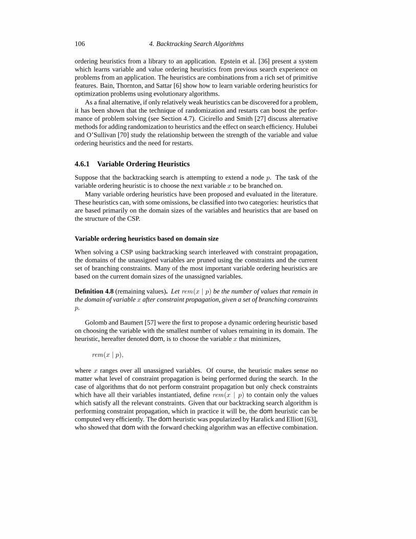
When solving a CSP using backtracking search interleaved with constraint propagation,the domains of the unassigned variables are pruned using the constraints and the currentset of branching constraints. Many of the most important variable ordering heuristics arebased on the current domain sizes of the unassigned variables.

Definition 4.8 (remaining values). Let rem(x | p) be the number of values that remain inthe domain of variable x after constraint propagation, given a set of branching constraintsp.

Golomb and Baumert [57] were the first to propose a dynamic ordering heuristic basedon choosing the variable with the smallest number of values remaining in its domain. Theheuristic, hereafter denoted dom, is to choose the variable x that minimizes,

rem(x | p),

where x ranges over all unassigned variables. Of course, the heuristic makes sense nomatter what level of constraint propagation is being performed during the search. In thecase of algorithms that do not perform constraint propagation but only check constraintswhich have all their variables instantiated, define rem(x | p) to contain only the valueswhich satisfy all the relevant constraints. Given that our backtracking search algorithm isperforming constraint propagation, which in practice it will be, the dom heuristic can becomputed very efficiently. The dom heuristic was popularized by Haralick and Elliott [63],who showed that dom with the forward checking algorithm was an effective combination.

P. van Beek 107

Much effort has gone into understanding this simple but effective heuristic. Intrigu-ingly, Golomb and Baumert [57], when first proposing dom, state that from an information-theoretic point of view, it can be shown that on average choosing the variable with thesmallest domain size is more efficient, but no further elaboration is provided. Haralick andElliott [63] show analytically that dom minimizes the depth of the search tree, assuminga simplistic probabilistic model of a CSP and assuming that we are searching for all so-lutions using a forward checking algorithm. Nudel [105], shows that dom is optimal (itminimizes the number of nodes in the search tree) again assuming forward checking butusing a slightly more refined probabilistic model. Gent et al. [52] propose a measure calledkappa whose intent is to capture “constrainedness” and what it means to choose the mostconstrained variable first. They show that dom (and dom+deg, see below) can be viewedas an approximation of this measure.

Hooker [66], in an influential paper, argues for the scientific testing of heuristics—asopposed to competitive testing—through the construction of empirical models designed tosupport or refute the intuition behind a heuristic. Hooker and Vinay [67] apply the method-ology to the study of the Jeroslow-Wang heuristic, a variable ordering heuristic for SAT.Surprisingly, they find that the standard intuition, that “a [heuristic] performs better whenit creates subproblems that are more likely to be satisfiable,” is refuted whereas a newlydeveloped intuition, that “a [heuristic] works better when it creates simpler subproblems,”is confirmed. Smith and Grant [120] apply the methodology to the study of dom. Haralickand Elliott [63] proposed an intuition behind the heuristic called the fail-first principle: “tosucceed, try first where you are most likely to fail”. Surprisingly, Smith and Grant find thatif one equates the fail-first principle with minimizing the depth of the search tree, as Har-alick and Elliott did, the principle is refuted. In follow on work, Beck et al. [14] find that ifone equates the fail-first principle with minimizing the number of nodes in the search tree,as Nadel did, the principle is confirmed. Wallace [132], using a factor analysis, finds twobasic factors behind the variation in search efficiency due to variable ordering heuristics:immediate failure and future failure.

In addition to the effort that has gone into understanding dom, much effort has goneinto improving it. Brelaz [20], in the context of graph coloring, proposes a now widelyused generalization of dom. Let the degree of an unassigned variable x be the numberof constraints which involve x and at least one other unassigned variable. The heuristic,hereafter denoted dom+deg, is to choose the variable with the smallest number of valuesremaining in its domain and to break any ties by choosing the variable with the highestdegree. Note that the degree information is dynamic and is updated as variables are instan-tiated. A static version, where the degree information is only computed prior to search, isalso used in practice.

Bessiere and Regin [17] propose another generalization of dom. The heuristic, here-after denoted dom/deg, is to divide the domain size of a variable by the degree of thevariable and to choose the variable which has the minimal value. The heuristic is shown towork well on random problems. Boussemart et al. [19] propose to divide by the weighteddegree, hereafter denoted dom/wdeg. A weight, initially set to one, is associated witheach constraint. Every time a constraint is responsible for a deadend, the associated weightis incremented. The weighted degree is the sum of the weights of the constraints whichinvolve x and at least one other unassigned variable. The dom/wdeg heuristic is shown towork well on a variety of problems. As an interesting aside, it has also been shown empir-ically that arc consistency propagation plus the dom/deg or the dom/wdeg heuristic can


reduce or remove the need for backjumping on some problems [17, 84].Gent et al. [50] propose choosing the variable x that minimizes,

rem(x | p)∏C

(1 − tC),

where C ranges over all constraints which involve x and at least one other unassigned vari-able and tC is the fraction of assignments which do not satisfy the constraint C. They alsopropose other heuristics which contain the product term in the above equation. A limitationof all these heuristics is the requirement of an updated estimate of tC for each constraintC as the search progresses. This is clearly costly, but also problematic for intensionallyrepresented constraints and non-binary constraints. As well, the product term implicitlyassumes that the probability a constraint fails is independent, an assumption that may nothold in practice.

Brown and Purdom [21] propose choosing the variable x that minimizes,

rem(x | p) + miny �=x

⎧⎨⎩∑

a∈rem(x|p)rem(y | p ∪ {x = a})

⎫⎬⎭ ,

where y ranges over all unassigned variables. The principle behind the heuristic is to pickthe variable x that is the root of the smallest 2-level subtree. Brown and Purdom show thatthe heuristic works better than dom on random SAT problems as the problems get larger.However, the heuristic has yet to be thoroughly evaluated on hard SAT problems or generalCSPs.

Geelen [49] proposes choosing the variable x that minimizes,∑a∈dom(x)

∏y

rem(y | p ∪ {x = a}),

where y ranges over all unassigned variables. The product term can be viewed as an upperbound on the number of solutions given a value a for x, and the principle behind theheuristic is said to be to choose the most “constrained” variable. Geelen shows that theheuristic works well on the n-queens problem when the level of constraint propagationused is forward checking. Refalo [111] proposes a similar heuristic and shows that it ismuch better than dom-based heuristics on multi-knapsack and magic square problems.Although the heuristic is costly to compute, Refalo’s work shows that it can be particularlyuseful in choosing the first, or first few variables, in the ordering. Interestingly, Wallace[132] reports that on random and quasigroup problems, the heuristic does not perform well.

Freeman [38], in the context of SAT, proposes choosing the variable x that minimizes,∑a∈dom(x)

∑y

rem(y | p ∪ {x = a}),

where y ranges over all unassigned variables. Since this is an expensive heuristic, Free-man proposes using it primarily when choosing the first few variables in the search. Theprinciple behind the heuristic is to maximize the amount of propagation and the number ofvariables which become instantiated if the variable is chosen, and thus simplify the remain-ing problem. Although costly to compute, Freeman shows that the heuristic works well on

P. van Beek 109

hard SAT problems when the level of constraint propagation used is unit propagation, theequivalent of forward checking. Malik et al. [91] show that a truncated version (using justthe first element in dom(x)) is very effective in instruction scheduling problems.

Structure-guided variable ordering heuristics

A CSP can be represented as a graph. Such graphical representations form the basis ofstructure-guided variable ordering heuristics. Real problems often do contain much struc-ture and on these problems the advantages of structure-guided heuristics include that struc-tural parameters can be used to bound the worst-case of a backtracking algorithm andstructural goods and nogoods can be recorded and used to prune large parts of the searchspace. Unfortunately, a current limitation of these heuristics is that they can break down inthe presence of global constraints, which are common in practice. A further disadvantageis that some structure-guided heuristics are either static or nearly static.

Freuder [40] may have been the first to propose a structure-guided variable orderingheuristic. Consider the constraint graph where there is a vertex for each variable in theCSP and there is an edge between two vertices x and y if there exists a constraint C suchthat both x ∈ vars(C) and y ∈ vars(C).

Definition 4.9 (width). Let the vertices in a constraint graph be ordered. The width of anordering is the maximum number of edges from any vertex v to vertices prior to v in theordering. The width of a constraint graph is the minimum width over all orderings of thatgraph.

Consider the static variable ordering corresponding to an ordering of the vertices in thegraph. Freuder [40] shows that the static variable ordering is backtrack-free if the levelof strong k-consistency is greater than the width of the ordering. Clearly, such a variableordering is within an O(d) factor of an optimal ordering, where d is the size of the domain.Freuder [40] also shows that there exists a backtrack-free static variable ordering if thelevel of strong consistency is greater than the width of the constraint graph. Freuder [41]generalizes these results to static variable orderings which guarantee that the number ofnodes visited in the search can be bounded a priori.

Dechter and Pearl [35] propose a variable ordering which first instantiates variableswhich cut cycles in the constraint graph. Once all cycles have been cut, the constraintgraph is a tree and can be solved quickly using arc consistency [40]. Sabin and Freuder[117] refine and test this proposal within an algorithm that maintains arc consistency. Theyshow that, on random binary problems, a variable ordering that cuts cycles can out performdom+deg.

Zabih [136] proposes choosing a static variable ordering with small bandwidth. Letthe n vertices in a constraint graph be ordered 1, . . . , n. The bandwidth of an ordering isthe maximum distance between any two vertices in the ordering that are connected by anedge. The bandwidth of a constraint graph is the minimum bandwidth over all orderingsof that graph. Intuitively, a small bandwidth ordering will ensure that variables that causedthe failure will be close by and thus reduce the need for backjumping. However, there iscurrently little empirical evidence that this is an effective heuristic.

A well-known technique in algorithm design on graphs is divide-and-conquer usinggraph separators.


Definition 4.10 (separator). A separator of a graph is a subset of the vertices or the edgeswhich, when removed, separates the graph into disjoint subgraphs.

A graph can be recursively decomposed by successively finding separators of the re-sulting disjoint subgraphs. Freuder and Quinn [42] propose a variable ordering heuristicbased on a such a recursive decomposition. The idea is that the separators (called cutsets in[42]) give groups of variables which, once instantiated, decompose the CSP. Freuder andQuinn also propose a special-purpose backtracking algorithm to correctly use the variableordering to get additive behavior rather than multiplicative behavior when solving the inde-pendent problems. Huang and Darwiche [69] show that the special-purpose backtrackingalgorithm is not needed; one can just use CBJ. Because the separators are found prior tosearch, the pre-established variable groupings never change during the execution of thebacktracking search. However, Huang and Darwiche note that within these groupings thevariable ordering can be dynamic and any one of the existing variable ordering heuristicscan used. Li and van Beek [86] present several improvements to this divide-and-conquerapproach. So far the divide-and-conquer approach has been shown to be effective on hardSAT problems [69, 86], but there has as yet been no systematic evaluation of the approachon general CSP problems.

As two final structure-guided heuristics, Moskewicz et al. [103], in their Chaff solverfor SAT, propose that the choice of variable should be biased towards variables that occurin recently recorded nogoods. Jegou and Terrioux [73] use a tree-decomposition of theconstraint graph to guide the variable ordering.

4.6.2 Value Ordering Heuristics

Suppose that the backtracking search is attempting to extend a node p and the variableordering heuristic has chosen variable x to be branched on next. The task of the valueordering heuristic is to choose the next value a for x. The principle being followed in thedesign of many value ordering heuristics is to choose next the value that is most likely tosucceed or be a part of a solution. Value ordering heuristics have been proposed whichare based on either estimating the number of solutions or estimating the probability of asolution, for each choice of value a for x. Clearly, if we knew either of these propertiesexactly, then a perfect value ordering would also be known—simply select a value thatleads to a solution and avoid a value that does not lead to a solution.

Dechter and Pearl [35] propose a static value ordering heuristic based on approximatingthe number of solutions to each subproblem. An approximation of the number of solutionsis found by forming a tree relaxation of the problem, where constraints are dropped untilthe constraint graph of the CSP can be represented as a tree. Counting all solutions to atree-structured CSP is polynomial and thus can be computed exactly. The values are thenordered by decreasing estimates of the solution counts. Followup work [76, 94, 131] hasfocused on generalizing the approach to dynamic value orderings and on improving theapproximation of the number of solutions (the tree relaxation can provide a poor estimateof the true solution count) by using recent ideas from Bayesian networks. A limitationof this body of work is that, while it compares the number of solutions, it does not takeinto account the size of the subtree that is being branched into or the difficultly or cost ofsearching the subtree.

P. van Beek 111

Ginsberg et al. [55], in experiments which used crossword puzzles as a test bed, proposethe following dynamic value ordering heuristic. To instantiate x, choose the value a ∈dom(x) that maximizes the product of the remaining domain sizes,

∏y

rem(y | p ∪ {x = a}),

where y ranges over all unassigned variables. Ginsberg et al. show that the heuristic workswell on crossword puzzles when the level of constraint propagation used is forward check-ing. Further empirical evidence for the usefulness of this heuristic was provided by Geelen[49]. Geelen notes that the product gives the number of possible completions of the nodep and these completions can be viewed in two ways. First, assuming that every comple-tion is equally likely to be a solution, choosing the value that maximizes the product alsomaximizes the probability that we are branching into a subproblem that contains a solution.Second, the completions can be viewed as an upper bound on the number of solutions to thesubproblem. Frost and Dechter [46] propose choosing the value that maximizes the sumof the remaining domain sizes. However, Geelen [49] notes that the product differentiatesmuch better than summation. In the literature, the product heuristic is sometimes called the“promise” heuristic and the summation heuristic is sometimes called the “min-conflicts”heuristic—as it was inspired by a local search heuristic of the same name proposed by

Minton et al. [99].

4.7 Randomization and Restart Strategies

It has been widely observed that backtracking algorithms can be brittle on some instances.Seemingly small changes to a variable or value ordering heuristic, such as a change inthe ordering of tie-breaking schemes, can lead to great differences in running time. Anexplanation for this phenomenon is that ordering heuristics make mistakes. Depending onthe number of mistakes and how early in the search the mistakes are made (and thereforehow costly they may be to correct), there can be a large variability in performance betweendifferent heuristics. A technique called randomization and restarts has been proposed fortaking advantage of this variability.

The technique of randomization and restarts within backtracking search algorithmsgoes back at least to the PhD work of Harvey [64]. Harvey found that periodically restart-ing a backtracking search with different variable orderings could eliminate the problemof “early mistakes”. This observation led Harvey to propose randomized backtrackingalgorithms where on each run of the backtracking algorithm the variable or the value or-derings are randomized. The backtracking algorithm terminates when either a solutionhas been found or the distance that the algorithm has backtracked from a deadend ex-ceeds some fixed cutoff. In the latter case, the backtracking algorithm is restarted and thesearch begins anew with different orderings. Harvey shows that this randomize and restarttechnique gives improved performance over a deterministic backtracking algorithm on jobshop scheduling problems. Gomes et al. [60, 61, 62] have done much to popularize and ad-vance the technique through demonstrations of its wide applicability, drawing connectionsto closely related work on Las Vegas algorithms, and contributions to our understanding ofwhen and why restarts help.


In the rest of this section, I first survey work on the technique itself and then surveywork that addresses the question of when do restarts help. For more on the topic of ran-domization and restart strategies see, for example, the survey by Gomes [58].

4.7.1 Algorithmic Techniques

The technique of randomization and restarts requires a method of adding randomizationto a deterministic backtracking algorithm and a restart strategy, a schedule or method fordeciding when to restart.

Randomization

Several possible methods of adding randomization to backtracking algorithms have beenproposed in the literature. Harvey [64] proposes randomizing the variable ordering. Gomeset al. [61, 62] propose randomizing the variable ordering heuristic either by randomized tiebreaking or by ranking the variables using an existing heuristic and then randomly choos-ing a variable from the set of variables that are within some small factor of the best variable.They show that restart strategies with randomized variable orderings lead to orders of mag-nitude improvement on a wide variety of problems including both SAT and CSP versionsof scheduling, planning, and quasigroup completion problems. Cicirello and Smith [27]discuss alternative methods for adding randomization to heuristics and the effect on searchefficiency. Other alternatives are to choose a variable with a probability that is propor-tional to the heuristic weight of the variable or to randomly pick from among a suite ofheuristics. One pitfall to be aware of is that the method of adding randomization to theheuristic must give enough different decisions near the top of the search tree. Harvey [64]proposes randomizing the value ordering so that each possible ordering is equally likely.As well, all the options listed above for randomizing variable orderings are also optionsfor value orderings. Zhang [138] argues that randomizing a heuristic can weaken it, anundesirable effect. Prestwich [106] and Zhang [138] propose a random backwards jump inthe search space upon backtracking. Although effective, this has the consequence that thebacktracking algorithm is no longer complete.

Restart strategies

A restart strategy S = (t1, t2, t3, ...) is an infinite sequence where each ti is either a pos-itive integer or infinity. The idea is that the randomized backtracking algorithm is run fort1 steps. If no solution is found within that cutoff, the algorithm is run for t 2 steps, and soon. A fixed cutoff strategy is a strategy where all the t i are equal. Various restart strategieshave been proposed.

Luby, Sinclair, and Zuckerman [88] (hereafter just Luby) examine restart strategies inthe more general setting of Las Vegas algorithms. A Las Vegas algorithm is a randomizedalgorithm that always gives the correct answer when it terminates, however the runningtime of the algorithm varies from one run to another and can be modeled as a randomvariable. Let f(t) be the probability that a backtracking algorithm A applied to instancex stops after taking exactly t steps. Let F (t) be the cumulative distribution function of f ;i.e., the probability that A stops after taking t or fewer steps. F (t) is sometimes referredto as the runtime distribution of algorithm A on instance x. The tail probability is the

P. van Beek 113

probability that A stops after taking more than t steps; i.e., 1 − F (t), which is sometimesreferred to as the survival function. Luby shows that, given full knowledge of the runtimedistribution, the optimal strategy is given by S t∗ = (t∗, t∗, t∗, . . .), for some fixed cutofft∗. Of course, the runtime distribution is not known in practice. For the case where thereis no knowledge of the runtime distribution, Luby shows that a universal strategy givenby Su = (1, 1, 2, 1, 1, 2, 4, 1, 1, 2, 1, 1, 2, 4, 8, 1, . . .) is within a log factor of the optimalstrategy St∗ and that this is the best performance that can be achieved up to a constantfactor by any universal strategy. Further, Luby proves that, no matter what the runtimedistribution of the original algorithm A, if we apply A using restart strategy S t∗ or Su, thetail probability of the restart strategy is small as it decays exponentially.

To use a restart strategy in practice, one must decide what counts as a primitive oper-ation or step in the computation. Several methods have been used in the literature. Har-vey [64] uses a fixed cutoff strategy which restarts the backtracking algorithm when thedistance that the algorithm has backtracked from a deadend exceeds some fixed cutoff.Richards [112] restarts at every deadend, but maintains completeness by first recording anogood so the deadend is not revisited. Gomes et al. [61] use a fixed cutoff strategy thatrestarts the backtracking algorithm when the number of backtracks exceeds some fixed cut-off. Kautz et al. [78, 115] use the number of nodes visited by the backtracking algorithm.For a fixed cutoff strategy, one must also decide what cutoff to use. So far it appears thatgood cutoffs are specific to an instance. Thus one must perform some sort of trial-and-errorsearch for a good cutoff value. However, van Moorsel and Wolter [130] observe that forsome runtime distributions a wide range of cutoffs perform well. They further observe thatit is often safer to make the cutoff too large rather than too small. For the universal strategy,one does not need to decide the cutoff. However, it has been reported that the universalstrategy is slow in practice as the sequence increases too slowly (e.g., [61, 78, 115]). Notethat this does not contradict the fact that the universal strategy is within a log factor ofoptimal, since this is an asymptotic result and ignores constant factors. However, it mayalso be noted that one can scale the universal strategy Su = (s, s, 2s, . . .), for some scalefactor s, and possibly improve performance while retaining the optimality guarantee.

Walsh [134] proposes a universal strategy Sg = (1, r, r2, . . .), where the restart valuesare geometrically increasing, and shows that values of r in the range 1 < r < 2 work wellon the problems examined. The strategy has the advantage that it increases more quicklythan the universal strategy but avoids the search for a cutoff necessary for a fixed cutoffstrategy. Although it appears to work well in practice, unfortunately the geometric strategycomes with no formal guarantees for its worst-case performance. It can be shown that theexpected runtime of the geometric strategy can be arbitrarily worse than that of the optimalstrategy.

Kautz et al. [78, 115] (hereafter just Kautz) observe that Luby makes two assumptionswhen proving the optimality of St∗ that may not hold in practice. The assumptions are (i)that successive runs of the randomized algorithm are statistically independent and identi-cally distributed, and (ii) that the only feasible observation or feature is the length of a run.As an example of where the first assumption may be false, consider the case where the cur-rent instance is drawn from one of two distributions but we do not know which. The failureto find a solution in previous runs can change our belief about the runtime distribution ofthe current instance. To show that the second assumption may be false, Kautz shows thata Bayesian model based on a rich set of features can with sufficient accuracy predict theruntime of the algorithm on the current instance. Kautz removes these assumptions and


proposes context-sensitive or dynamic restart strategies. In one set of experiments, Kautzshows that a dynamic strategy can do better than the static optimal strategy S t∗ . The strat-egy uses a Bayesian model to predict whether a current run of the algorithm will be either“long” or “short”, and restarts if the prediction is “long”.

Van Moorsel and Wolter [130] consider a case that often arises in practice where asolution is useful only if it is found within some deadline; i.e., we are given a deadlinec and we may run the restart strategy until a total of c steps of the algorithm have beenexecuted. Van Moorsel and Wolter consider restart strategies that maximize the probabilitythe deadline is met.

4.7.2 When Do Restarts Help?

The question of when and why the technique of randomization and restarts is useful hasbeen addressed from two angles: For what kinds of runtime distributions are restarts help-ful and what are the underlying causes for these runtime distributions.

Runtime distributions for which restarts are useful

In the case where restarts are helpful on satisfiable instances, Gomes et al. [61, 62] showthat probability distributions with heavy-tails can be a good fit to the runtime distribu-tions of backtracking algorithms with randomized heuristics. A heavy-tailed distributionis one where the tail probability or survival function (see above) decays polynomially;i.e., there is a significant probability that the backtracking algorithm will run for a longtime. For unsatisfiable instances, Gomes et al. [61] report that in their experiments onrandom quasigroup completion problems, heavy-tailed behavior was not found and thatrestarts were consequently not helpful on these problems. As an interesting aside, Bap-tista and Marques-Silva [8] show experimentally that—because of synergy between thetechniques—a backtracking algorithm that incorporates nogood recording can benefit fromrandomization and restarts when solving unsatisfiable instances.

Hoos [68] notes that restarts will not only be effective for heavy tails, but that its effec-tiveness depends solely on there existing some point where the cumulative runtime distri-bution is increasing slower than the exponential distribution. It is at this point, where thesearch is stagnating, that a restart would be helpful.

Van Moorsel and Wolter [129] provide necessary and sufficient conditions for restartsto be helpful. Their work can be seen as a formalization of Hoos’ insight and its exten-sion from one restart to multiple restarts. Let T be a random variable which models theruntime of a randomized backtracking algorithm on an instance and let E[T ] be the ex-pected value of T . Under the assumption that successive runs of the randomized algorithmare statistically independent and identically distributed, Van Moorsel and Wolter show thatany number of restarts using a fixed cutoff of t steps is better than just letting the algorithmrun to completion if and only if,

E[T ] < E[T − t | T > t]

holds; i.e., if and only if the expected runtime of the algorithm is less than the expectedremaining time to completion given that the algorithm has run for t steps. Van Moorsel andWolter also show that if a single restart improves the expected runtime, multiple restarts

P. van Beek 115

perform even better, and unbounded restarts performs best. For what kinds of distribu-tions does the above condition hold? Restarts will be most effective (the inequality willbe greatest) for heavy-tailed distributions, where the tail decays polynomially, but VanMoorsel and Wolter observe that the condition also hold for some distributions where thetail decays exponentially. For other exponentially decaying distributions, restarting willbe strictly worse than running the algorithm to completion. Zhan [137] shows that this isnot an isolated case and for many problems restarts can be harmful. For pure exponentialdistributions, the condition is an equality and restarts will be neither helpful or harmful.

Underlying causes for these runtime distributions

Various theories have been postulated for explaining why restarts are helpful; i.e., why doruntime distributions arise where restarts are helpful. It is superficially agreed that an ex-planation for this phenomenon is that ordering heuristics make mistakes which require thebacktracking algorithm to explore large subtrees with no solutions. However, the theoriesdiffer in what it means for an ordering heuristic to make a mistake.

Harvey [64] defines a mistake as follows.

Definition 4.11 (value mistake). A mistake is a node in the search tree that is a nogoodbut the parent of the node is not a nogood.

When a mistake is made, the search has branched into a subproblem that does nothave a solution. The result is that the node has to be refuted and doing this may requirea large subtree to be explored, especially if the mistake is made early in the tree. In thisdefinition, value ordering heuristics make mistakes, variable ordering heuristics do not.However, changing the variable ordering can mean either that a mistake is not made, sincethe value ordering is correct for the newly chosen variable, or that any mistake is less costlyto correct. Harvey constructs a probabilistic model to predict when a restart algorithm willperform better than its deterministic counterpart. With simplifying assumptions about theprobability of a mistake, it is shown that restarts are beneficial when the mistake probabilityis small. Clearly, the definition, and thus the probabilistic model on which it depends, onlyapplies if a CSP has a solution. Therefore, the theory does not explain when restarts wouldbe beneficial for unsatisfiable problems.

As evidence in support of this theory, Hulubei and O’Sullivan [70] consider the dis-tribution of refutation sizes to correct mistakes (the size of the subtrees that are rooted atmistakes). They show that when using a poor value ordering in experiments on quasigroupcompletion problems, heavy-tailed behavior was observed for every one of four differenthigh-quality variable ordering heuristics. However, the heavy-tailed behavior disappearedwhen the same experiments were performed but this time with a high-quality value order-ing heuristic in place of the random value ordering.

Williams, Gomes, and Selman [135] (hereafter just Williams) define a mistake as fol-lows.

Definition 4.12 (backdoor mistake). A mistake is a selection of a variable that is not in aminimal backdoor, when such a variable is available to be chosen.

A backdoor is a set of variables for which there exists value assignments such that thesimplified problem (such as after constraint propagation) can be solved in polynomial time.Backdoors capture the intuition that good variable and value ordering heuristics simplify


the problem as quickly as possible. When a mistake is made, the search has branched intoa subproblem that has not been as effectively simplified as it would have been had it chosena backdoor variable. The result is that the subproblem is more costly to search, especiallyif the mistake is made early in the tree. In this definition, variable ordering heuristicsmake mistakes, value ordering heuristics do not. Williams constructs a probabilisticmodel to predict when heavy-tailed behavior will occur but there will exist a restart strategythat will have polynomial expected running time. With simplifying assumptions about theprobability of a mistake, it is shown that both of these occur when the probability of amistake is sufficiently small and the size of the minimal backdoor is sufficiently small.The theory can also explain when restarts would be beneficial for unsatisfiable problems,through the notion of a strong backdoor. However, the theory does not entirely account forthe fact that a random value ordering together with a restart strategy can remove heavy-tail behavior. In this case the variable ordering remains fixed and so the probability of amistake also remains unchanged.

Finally, some work contributes to our understanding of why runtime distributions arisewhere restarts are helpful while remaining agnostic about the exact definition of a mistake.Consider the probability distribution of refutation sizes to correct mistakes. It has beenshown both empirically on random problems and through theoretical, probabilistic modelsthat heavy-tails arise in the case where this distribution decays exponentially as the sizeof the refutation grows [24, 59]. In other words, there is an exponentially decreasingprobability of making a costly (exponentially-sized) mistake.

4.8 Best-First Search

In the search tree that is traversed by a backtracking algorithm, the branches out of anode are assumed to be ordered by a value ordering heuristic, with the left-most branchbeing the most promising (or at least no less promising than any branch to the right). Thebacktracking algorithm then performs a depth-first traversal of the search tree, visitingthe branches out of a node in left-to-right order. When a CSP instance is unsatisfiableand the entire search tree must be traversed, depth-first search is the clear best choice.However, when it is known or it can safely be assumed that a CSP instance is satisfiable,alternative search strategies such as best-first search become viable. In this section, Isurvey discrepancy-based search strategies, which can be viewed as variations on best-firstsearch.

Harvey and Ginsberg [64, 65] were the first to propose a discrepancy-based searchstrategy, in an algorithm called limited discrepancy search. A discrepancy is the casewhere the search does not follow the value ordering heuristic and does not take the left-most branch out of a node. The idea behind limited discrepancy search is to iterativelysearch the tree by increasing number of discrepancies, preferring discrepancies that occurnear the root of the tree. This allows the search to recover from mistakes made early in thesearch (see Definition 4.11). In contrast, with backtracking (or depth-first) search, mistakesmade near the root of the tree can be costly to discover and undo. On the i th iteration, thelimited discrepancy algorithm visits all leaf nodes with up to i discrepancies in the pathfrom the root to the leaf. The algorithm terminates when a solution is found or the iterationis exhausted. Limited discrepancy search is called iteratively with i = 0, 1, . . . , k. Ifk ≥ n, where n is the depth of the search tree, the algorithm is complete; otherwise it is

P. van Beek 117

incomplete. Harvey and Ginsberg show both theoretically and experimentally that limiteddiscrepancy search can be better than depth-first search on satisfiable instances when agood value ordering heuristic is available.

Korf [80] proposes a modification to the limited discrepancy algorithm so that it visitsfewer duplicate nodes on subsequent iterations. On the i th iteration, Korf’s algorithm visitsall leaf nodes with exactly i discrepancies in the path from the root to the leaf. However, toachieve these savings, Korf’s algorithm prefers discrepancies deeper in the tree. Korf notesthat limited discrepancy search can be viewed as a variation on best-first search, where thecost of a node p is the number of discrepancies in the path from the root of the search treeto p. In best-first search, the node with the lowest cost is chosen as the next node to beextended. In Harvey and Ginsberg’s proposal, ties for lowest cost are broken by choosinga node that is closest to the root. In Korf’s proposal, ties are broken by choosing a nodethat is farthest from the root.

Walsh [133] (and independently Meseguer [95]), argues that value ordering heuris-tics tend to be less informed and more prone to make mistakes near the top of the searchtree. Walsh proposes depth-bounded discrepancy search, which biases search to discrep-ancies near the top of the tree, but visits fewer redundant nodes than limited discrepancysearch. On the ith iteration, the depth-bounded discrepancy search algorithm visits allleaf nodes where all discrepancies in the path from the root to the leaf occur at depth i orless. Meseguer [95] proposes interleaved depth-first search, which also biases search todiscrepancies near the top of the tree. The basic idea is to divide up the search time on thebranches out of a node using a variation of round-robin scheduling. Each branch—or moreproperly, each subtree rooted at a branch—is searched for a given time-slice using depth-first search. If no solution is found within the time slice, the search is suspended and thenext branch becomes active. Upon suspending search in the last branch, the first branchagain becomes active. This continues until either a solution is found or all the subtreeshave been exhaustively searched. The strategy can be applied recursively within subtrees.

Meseguer and Walsh [96] experimentally compare backtracking algorithms using tradi-tional depth-first search and the four discrepancy-based search strategies described above.On a test bed which consisted of random binary, quasigroup completion, and number par-titioning CSPs, it was found that discrepancy-based search strategies could be much bet-ter than depth-first search. As with randomization and restarts, discrepancy-based searchstrategies are a way to overcome value ordering mistakes made early in the search.

4.9 Optimization

In some important application areas of constraint programming such as scheduling, se-quencing and planning, CSPs arise which have, in addition to constraints which must besatisfied, an objective function f which must be optimized. Without loss of generality, Iassume in what follows that the goal is to find a solution which minimizes f and that f isa function over all the variables of the CSP. I also assume that a variable c has been addedto the CSP model and constrained to be equal to the objective function; i.e., c = f(X),where X is the set of variables in the CSP. I call this the objective constraint.

To solve optimization CSPs, the common approach is to find an optimal solution bysolving a sequence of CSPs; i.e., a sequence of satisfaction problems. Several variationshave been proposed and evaluated in the literature. Van Hentenryck [128] proposes what


can be viewed as a constraint-based version of branch-and-bound. Initially, a backtrackingsearch is used to find any solution p which satisfies the constraints. A constraint is thenadded to the CSP of the form c < f(S) which excludes solutions that are not better thanthis solution. A new solution is then found for the augmented CSP. This process is repeateduntil the resulting CSP is unsatisfiable, in which case the last solution found has beenproven optimal. Baptiste, Le Pape, and Nuijten [9] suggest iterating on the possible valuesof c by either (i) iterating from the smallest value in dom(c) to the largest until a solutionis found, (ii) iterating from largest to smallest until a solution is no longer found, or (iii)performing binary search. Each time, of course, we are solving a satisfaction problemusing a backtracking search algorithm. For these approaches to be effective, it is importantthat constraint propagation techniques be applied to the objective constraint. For example,see [9, Chapter 5] for propagation techniques for objective constraints for several objectivefunctions that arise in scheduling.

4.10 Comparing Backtracking Algorithms

As this survey has indicated, many improvements to backtracking have been proposed andthere are many ways that these techniques can be combined together into one algorithm. Inthis section, I survey work on comparing the performance of backtracking algorithms. Thework is categorized into empirical and theoretical approaches. Both approaches have well-known advantages and disadvantages. Empirical comparisons allow the comparison of anypair of backtracking algorithms, but any conclusion about which algorithm is better willalways be weak since it must be qualified by the phrase, “on the instances we examined”.Theoretical comparisons allow categorical statements about the relative performance ofsome pairs of backtracking algorithms, but the requirement that any conclusion be true forall instances means that statements cannot be made about every pair of algorithms and thestatements that can be made must sometimes be necessarily weak.

When comparing backtracking algorithms, several performance measures have beenused. For empirical comparisons, of course runtime can be used, although this requiresone to be sure that one is comparing the underlying algorithms and not implementationskill or choice of programming language. Three widely used performance measures thatare implementation independent are number of constraint checks, backtracks, and nodesvisited.

4.10.1 Empirical Comparisons

Early work in empirical comparisons of backtracking algorithms was hampered by a lackof realistic or hard test problems (e.g., [21, 48, 63, 93, 108, 114]). The experimental testbed often consisted of only toy problems—the ubiquitous n-queens problem first used in1965 [57] was still being used as a test bed more than 20 years later [125]—and simplerandom problems. As well, often only CSPs with binary constraints were experimentedupon. The focus on simple, binary CSPs was sometimes detrimental to the field and led topromising approaches being prematurely dismissed.

The situation improved with the discovery of hard random problems that arise at aphase transition and the investigation of alternative random models of CSPs (see [51] andreferences therein). Experiments could now be performed which compared the algorithms

P. van Beek 119

on the hardest problems and systematically explored the entire space of random problemsto see where one algorithm bettered another (e.g., [17, 45, 126]). Unfortunately, mostof the random models lack any structure or realism. The situation was further improvedby the realization that important applications of constraint programming are often bestmodeled using global constraints and other non-binary constraints, and the constructionand subsequent wide use of a constraint programming benchmark library [53].

In the remainder of this section, I review two representative streams of experiments:experiments that examine what level of constraint propagation a backtracking algorithmshould perform and experiments that examine the interaction between several techniquesfor improving a backtracking algorithm. Many other experiments—such as those per-formed by authors who have introduced a new technique and then show that the techniqueworks better on a selected set of test problems—are reported elsewhere in this survey.

Experiments on level of constraint propagation

Experiments have examined the question of what level of local consistency should be main-tained during the backtracking search. Consider the representative set of experiments sum-marized in Table 4.2. Gaschnig [47] originally proposed interleaving backtracking searchwith arc consistency. Early experiments which tested this proposal concluded that an algo-rithm that maintained arc consistency during the search was not competitive with forwardchecking [48, 63, 93].

This view was maintained for about fifteen years until it was challenged by Sabin andFreuder. Sabin and Freuder [116], using hard random problems, showed that MAC couldbe much better than forward checking. More recently, with an increasing emphasis on ap-plying constraint programming in practice, has come an understanding of the importance ofglobal constraints and other intensionally represented non-binary constraints for modelingreal problems. With such constraints, special purpose constraint propagation algorithmsare developed and the modeler has a choice of what level of constraint propagation toenforce. It is now generally accepted that the choice of level of constraint propagation de-pends on the application and different choices may be made for different constraints withinthe same CSP.

Table 4.2: Experiments on constraint propagation: MAC vs FC.

Faster? CommentMcGregor (1979) [93] FC 3 × fasterHaralick & Elliott (1980) [63] FC 3 × fasterSabin & Freuder (1994) [116] MAC much betterBacchus & van Run (1995) [5] FC 3–20 × fasterBessiere & Regin (1996) [17] MAC much betterLarrosa (2000) [81] both much better


Experiments on the interaction between improvements

Experiments have examined the interaction of the quality of the variable ordering heuris-tic, the level of local consistency maintained during the backtracking search, and the addi-tion of backjumping techniques such as conflict-directed backjumping (CBJ) and dynamicbacktracking (DBT). Unfortunately, these three techniques for improving a backtrackingalgorithm are not entirely orthogonal. Consider the representative set of experiments sum-marized in Table 4.3. These experiments show that, if the variable ordering is fixed andthe level of constraint propagation is forward checking, conflict-directed backjumping isan effective technique. However, it can also be observed in previous experimental workthat as the level of local consistency that is maintained in the backtracking search is in-creased and as the variable ordering heuristic is improved, the effects of CBJ are dimin-ished [5, 17, 107, 108]. For example, it can be observed in Prosser’s [108] experimentsthat, given a static variable ordering, increasing the level of local consistency maintainedfrom none to the level of forward checking, diminishes the effects of CBJ. Bacchus andvan Run [5] observe from their experiments that adding a dynamic variable ordering (animprovement over a static variable ordering) to a forward checking algorithm diminishesthe effects of CBJ. In their experiments the effects are so diminished as to be almost neg-ligible and they present an argument for why this might hold in general. Bessiere andRegin [17] observe from their experiments that simultaneously increasing the level of lo-cal consistency even further to arc consistency and further improving the dynamic variableordering heuristic diminishes the effects of CBJ so much that, in their implementation,the overhead of maintaining the data structures for backjumping actually slows down thealgorithm. They conjecture that when arc consistency is maintained and a good variableordering heuristic is used, “CBJ becomes useless”. All of the above experiments were onsmall puzzles—the Zebra problem and n-queens problem—and on random CSPs whichlacked any structure.

In contrast, in subsequent experiments on both random and real-world structured CSPs,backjumping was found to be a useful technique. Jussien, Debruyne, Boizumault [75]present empirical results that show that adding dynamic backtracking to an algorithm thatmaintains arc consistency can greatly improve performance. Chen and van Beek [26]present empirical results that show that, although the effects of CBJ may be diminished,adding CBJ to a backtracking algorithm that maintains arc consistency can still provideorders of magnitude speedups. Finally, CBJ is now a standard technique in the best back-tracking algorithms for solving structured SAT problems [83].

Table 4.3: Experiments on backjumping: FC vs FC-CBJ.

Faster? CommentRosiers and Bruynooghe (1987) [114] FC-CBJ never worseProsser (1993) [108] FC-CBJ three times betterFrost & Dechter (1994) [45] FC-CBJ somewhat betterBacchus & van Run (1995) [5] FC-CBJ slightlySmith & Grant (1995) [119] FC-CBJ sometimes much betterBayardo & Schrag (1996, 1997) [11, 12] FC-CBJ much better

P. van Beek 121

4.10.2 Theoretical Comparisons

Worst-case analysis and average-case analysis are two standard theoretical approaches tounderstanding and comparing algorithms. Unfortunately, neither approach has proven gen-erally successful for comparing backtracking algorithms. The worst-case bounds of back-tracking algorithms are always exponential and rarely predictive of performance, and theaverage-case analyses of backtracking algorithms have, by necessity, made simplifying andunrealistic assumptions about the distribution of problems (e.g., [63, 105, 110]).

Two alternative approaches that have proven more successful for comparing algorithmsare techniques based on proof complexity and a methodology for constructing partial or-ders based on characterizing properties of the nodes visited by an algorithm.

Proof complexity and backtracking algorithms

Backtracking algorithms can be compared using techniques from the proof complexity ofresolution refutation proofs. The results that can be proven are of the general form: Givenany CSP instance, algorithm A with an optimal variable and value ordering never visitsfewer and can visit exponentially more nodes when applied to the instance than algorithmB with an optimal variable and value ordering. The optimal orderings are relative to thealgorithms and thus A and B may use different orderings. I begin by briefly explainingresolution refutation proofs and proof complexity, followed by an explanation of someresults of applying proof complexity techniques to the study of backtracking algorithmsfor CSPs.

The resolution inference rule takes two premises in the form of clauses (A ∨ x) and(B ∨ ¬x) and gives the clause (A ∨ B) as a conclusion. The two premises are said tobe resolved and the variable x is said to be resolved away. Resolving the two clausesx and ¬x gives the empty clause. Given a set of input clauses F , a resolution proof orderivation of a clause C is a sequence of applications of the resolution inference rule suchthat C is the final conclusion and each premise in each application of the inference rule iseither a clause from F or a conclusion from a previous application of the inference rule. Aresolution proof that derives the empty clause is called a refutation proof, as it shows thatthe input set of clauses F is unsatisfiable.

A resolution proof of a clause C can be viewed as a directed acyclic graph (DAG).Each leaf node in the DAG is labeled with a clause from F , each internal node is labeledwith a derived clause that is justified by resolving the clauses of its two parents, and thereis a single node with no successors and the label of that node is C. Many restrictions onthe form of the proof DAG have been studied. For our purposes, one will suffice. A treeresolution proof is a resolution proof where the DAG of inferences forms a tree. The sizeof a proof is the number of nodes (clauses) in the proof DAG.

Proof complexity is the study of the size of the smallest proof a method can produce[28]. It is known that the smallest tree resolution refutation proof to show a set of clausesF is unsatisfiable can be exponentially larger than the smallest unrestricted resolution refu-tation proof and can never be smaller (see [13] and references therein). To see why treeproofs can be larger, note that if one wishes to use a derived clause elsewhere in the proofit must be re-derived. To see why tree proofs can never be smaller, note that every treeresolution proof is also an unrestricted resolution proof.


Why is resolution refutation proof complexity interesting for the study of backtrackingalgorithms? The search tree that results from applying a complete backtracking algorithmto an unsatisfiable CSP can be viewed as a resolution refutation proof. As an example ofthe correspondence, consider the backtracking tree that results from applying BT to theSAT problem which consists of the set of clauses {a ∨ b ∨ c, a ∨ ¬c, ¬b, ¬a ∨ c, b ∨ ¬c}.Each leaf node is labeled with the clause that caused the failure, interior nodes are labeledby working from the leaves to the root applying the resolution inference rule, and the rootwill be labeled with the empty clause. Thus, proof complexity addresses the question ofthe size of the smallest possible backtrack tree; i.e., the size of the backtrack tree if oneassumes optimal variable and value ordering heuristics.

The connection between backtracking algorithms for SAT and resolution has beenwidely observed and it is known that DPLL-based algorithms on unsatisfiable instancescorrespond to tree resolution refutation proofs. Baker [7] shows how to generalize this cor-respondence to the backtracking algorithm BT for general CSPs, when BT is using d-waybranching. Mitchell [100], using earlier work by de Kleer [32], shows how to generalizethis correspondence when BT is using 2-way branching.

Beame, Kautz, and Sabharwal [13] (hereafter Beame) use proof complexity techniquesto investigate backtracking algorithms with nogood recording. Let DPLL be a basic back-tracking algorithm for SAT, let DPLL+nr be DPLL with a nogood recording scheme (calledFirstNewCut) added, and let DPLL+nr+restarts be DPLL with nogood recording and in-finite restarts added. Beame shows that the smallest refutation proofs using DPLL can beexponentially longer than the smallest refutation proofs using DPLL+nr. In other words,DPLL with an optimal variable and value ordering never visits fewer and can visit expo-nentially more nodes than DPLL with nogood recording and an optimal variable and valueordering. Beame also shows that DPLL+nr+restarts is equivalent to unrestricted resolu-tion if the learned nogoods are retained between restarts. It is an open question whetherDPLL+nr is equivalent to unrestricted resolution or falls strictly between unrestricted res-olution and tree resolution proofs.

Hwang and Mitchell [71] use proof complexity techniques to investigate backtrack-ing algorithms with different branching strategies. Let BT-2-way be a basic backtrackingalgorithm for general CSPs using 2-way branching, and let BT-d-way be a backtrackingalgorithm using d-way branching. Hwang and Mitchell show that BT-d-way with an opti-mal variable and value ordering never visits fewer and can visit exponentially more nodesthan BT-2-way with an optimal variable and value ordering.

Although a powerful technique, a limitation of the proof complexity framework is thatit cannot be used to distinguish between some standard improvements to the basic chrono-logical backtracking algorithm. For example, consider the four combinations of addingor not adding unit propagation and conflict-directed backjumping to DPLL. When usingan optimal variable and value ordering each algorithm visits exactly the same number ofnodes. Similar results hold for adding conflict-directed backjumping, dynamic backtrack-ing, or forward checking to BT [7, 26, 100].

A partial order on backtracking algorithms

Backtracking algorithms can be compared by formulating necessary and sufficient condi-tions for a search tree node to be visited by each backtracking algorithm. These charac-terizations can then be used to construct a partial order (or hierarchy) on the algorithms

P. van Beek 123

according to two standard performance measures: the number of nodes visited and thenumber of constraint checks performed.

The results that can be proven are of the general form: Given any CSP instance andany variable and value ordering, algorithm A with the variable and value ordering nevervisits more nodes (and may visit fewer) when applied to the instance than algorithm B withthe same variable and value ordering. In other words, algorithm A dominates algorithm Bwhen the performance measure is nodes visited. A strong feature of this approach is thatthe results still hold (A still dominates B), even if the CSP model used by both algorithmsis the model that is best from algorithm B’s point of view and even if the variable and valueordering used by both algorithms are the orderings that are best (optimal) from algorithmB’s point of view.

Kondrak and van Beek [79] introduce the general methodology and give techniquesand definitions that can be used for characterizing backtracking algorithms. Using themethodology, they formulate necessary and sufficient conditions for several backtrackingalgorithms including BT, BJ, CBJ, FC, and FC-CBJ. As an example of a necessary condi-tion, it can be shown that if FC visits a node, then the parent of the node is 1-consistent (seeDefinition 4.3). As an example of a sufficient condition, it can be shown that if the parentof a node is 1-consistent, then BJ visits the node. The necessary and sufficient conditionscan then be used to order the two backtracking algorithms. For example, to show that FCdominates BJ in terms of nodes visited, we show that every node that is visited by FC isalso visited by BJ. The necessary condition for FC is used to deduce that the parent of thenode is 1-consistent. Since the parent of the node is 1-consistent, the sufficient conditionfor BJ can then be used to conclude that BJ visits the node.

Chen and van Beek [26] extend the partial ordering of backtracking algorithms to in-clude backtracking algorithms and their CBJ hybrids that maintain levels of local consis-tency beyond forward checking, including the algorithms that maintain arc consistency.To analyze the influence of the level of local consistency on the backjumping, Chen andvan Beek use the notion of backjump level. Informally, the level of a backjump is thedistance, measured in backjumps, from the backjump destination to the farthest deadend.By classifying the backjumps performed by a backjumping algorithm into different levels,CBJ is weakened into a series of backjumping algorithms which perform limited levels ofbackjumps. Let BJk be a backjumping algorithm which backjumps if the backjump levelj is less than or equal to k, but chronologically backtracks if j > k. BJn is equivalent toCBJ, which performs unlimited backjumps, and BJ1 is equivalent to Gaschnig’s [48] BJ,which only does first level backjumps. Recall that the maintaining strong k-consistencyalgorithm (MCk) enforces strong k-consistency at each node in the backtrack tree, whereMC1 is equivalent to FC and on binary CSPs MC2 is equivalent to MAC. MCk can be com-bined with backjumping, namely MCk-CBJ. Chen and van Beek show that an algorithmthat maintains strong k-consistency never visits more nodes than a backjumping algorithmthat is allowed to backjump at most k levels. Thus, as the level of local consistency thatis maintained in the backtracking search is increased, the less that backjumping will be animprovement.

Figure 4.3 shows a partial order or hierarchy in terms of the size of the backtrack treefor BJk, MCk, and MCk-CBJ. If there is a path from algorithm A to algorithm B in thefigure, A never visits more nodes than B. For example, for all variable orderings, MC k

never visits more nodes than BJj , for all j ≤ k.Bacchus and Grove [3] observe that the partial orderings with respect to nodes visited


can be extended to partial orderings with respect to constraint checks, or other measuresof the amount of work performed at each node. For example, on binary CSPs the MACalgorithm can perform O(n2d2) work at each node of the tree, where n is the number ofvariables and d is the size of the domain, whereas the FC algorithm can perform O(nd)work. Thus, one can conclude that on binary CSPs MAC can be at most O(nd) timesslower in the worst case (when the two algorithms visit the same nodes). The partialorderings with respect to nodes and constraint checks are consistent with and explain someof the empirical results reported in the literature (e.g., see the experiments reported inTables 4.2 & 4.3).

Besides the relationships that are shown explicitly, it is important to note the ones thatare implicit in the hierarchy. If there is not a path from algorithm A to algorithm B inthe hierarchy, A and B are incomparable. To show a pair of algorithms A and B areincomparable, one needs to find a CSP and a variable ordering on which A is better thanB, and one on which B is better than A. Examples have been given that cover all theincomparability results [4, 26, 79]. Some of the more surprising results include: CBJ andFC-CBJ are incomparable [79], CBJ and MCk are incomparable for any fixed k < n inthat each can be exponentially better than the other [4], and MAC-CBJ and FC-CBJ andmore generally MCk-CBJ and MCk+1-CBJ are incomparable for any fixed k < n in thateach can be exponentially better than the other [26].

P. van Beek 125

MCn BJn

(CBJ) MCn−CBJ

MCk+1 BJk+1 MCk+1−CBJ

MCk BJk MCk−CBJ

MC2

(MAC) BJ2

MC2−CBJ (MAC−CBJ)

MC1

(FC)

BJ1 (BJ)

MC1−CBJ (FC−CBJ)

BJ0 (BT)

Figure 4.3: A hierarchy for BJk , MCk, and MCk-CBJ in terms of the size of the backtracktree (adapted from [26, 79]). On binary CSPs, MC2 is equivalent to MAC and MC2-CBJis equivalent to MAC-CBJ.


Acknowledgements

I would like to thank Fahiem Bacchus, Xinguang Chen, Grzegorz Kondrak, Dennis Man-chak, and Jonathan Sillito for many interesting discussions and collaborations in the paston backtracking algorithms. I would also like to thank Christian Bessiere and George Kat-sirelos for helpful comments on an early draft of this survey. This work was supported inpart by the Natural Sciences and Engineering Research Council of Canada.

Bibliography

[1] F. Bacchus. Extending forward checking. In Proceedings of the Sixth InternationalConference on Principles and Practice of Constraint Programming, pages 35–51,Singapore, 2000.

[2] F. Bacchus. Enhancing Davis Putman with extended binary clause reasoning. InProceedings of the Eighteenth National Conference on Artificial Intelligence, pages613 – 619, Edmonton, 2002.

[3] F. Bacchus and A. Grove. On the forward checking algorithm. In Proceedings of theFirst International Conference on Principles and Practice of Constraint Program-ming, pages 292–309, Cassis, France, 1995.

[4] F. Bacchus and A. Grove. Looking forward in constraint satisfaction algorithms.Unpublished manuscript, 1999.

[5] F. Bacchus and P. van Run. Dynamic variable ordering in CSPs. In Proceedingsof the First International Conference on Principles and Practice of Constraint Pro-gramming, pages 258–275, Cassis, France, 1995.

[6] S. Bain, J. Thornton, and A. Sattar. Evolving variable-ordering heuristics for con-strained optimisation. In Proceedings of the Eleventh International Conference onPrinciples and Practice of Constraint Programming, pages 732–736, Sitges, Spain,2005.

[7] A. B. Baker. Intelligent Backtracking on Constraint Satisfaction Problems: Experi-mental and Theoretical Results. PhD thesis, University of Oregon, 1995.

[8] L. Baptista and J. Marques-Silva. Using randomization and learning to solve hardreal-world instances of satisfiability. In Proceedings of the Sixth International Con-ference on Principles and Practice of Constraint Programming, pages 489–494,Singapore, 2000.

[9] P. Baptiste, C. Le Pape, and W. Nuijten. Constraint-Based Scheduling: ApplyingConstraint Programming to Scheduling Problems. Kluwer, 2001.

[10] R. J. Bayardo Jr. and D. P. Miranker. A complexity analysis of space-boundedlearning algorithms for the constraint satisfaction problem. In Proceedings of theThirteenth National Conference on Artificial Intelligence, pages 298–304, Portland,Oregon, 1996.

[11] R. J. Bayardo Jr. and R. C. Schrag. Using CSP look-back techniques to solve excep-tionally hard SAT instances. In Proceedings of the Second International Conferenceon Principles and Practice of Constraint Programming, pages 46–60, Cambridge,Mass., 1996.

[12] R. J. Bayardo Jr. and R. C. Schrag. Using CSP look-back techniques to solve real-

P. van Beek 127

world SAT instances. In Proceedings of the Fourteenth National Conference onArtificial Intelligence, pages 203–208, Providence, Rhode Island, 1997.

[13] P. Beame, H. Kautz, and A. Sabharwal. Towards understanding and harnessing thepotential of clause learning. J. of Artificial Intelligence Research, 22:319–351, 2004.URL http://www.jair.org.

[14] J. C. Beck, P. Prosser, and R. J. Wallace. Trying again to fail first. In Recent Ad-vances in Constraints, Lecture Notes in Artificial Intelligence, Vol. 3419. Springer-Verlag, 2005.

[15] U. Bertele and F. Brioschi. Nonserial Dynamic Programming. Academic Press,1972.

[16] C. Bessiere, P. Meseguer, E. C. Freuder, and J. Larrosa. On forward checking fornon-binary constraint satisfaction. Artificial Intelligence, 141:205–224, 2002.

[17] C. Bessiere and J.-C. Regin. MAC and combined heuristics: Two reasons to for-sake FC (and CBJ?) on hard problems. In Proceedings of the Second InternationalConference on Principles and Practice of Constraint Programming, pages 61–75,Cambridge, Mass., 1996.

[18] C. Bliek. Generalizing partial order and dynamic backtracking. In Proceedings ofthe Fifteenth National Conference on Artificial Intelligence, pages 319–325, Madi-son, Wisconsin, 1998.

[19] F. Boussemart, F. Hemery, C. Lecoutre, and L. Sais. Boosting systematic search byweighting constraints. In Proceedings of the 16th European Conference on ArtificialIntelligence, pages 146–150, Valencia, Spain, 2004.

[20] D. Brelaz. New methods to color the vertices of a graph. Comm. ACM, 22:251–256,1979.

[21] C. A. Brown and P. W. Purdom Jr. An empirical comparison of backtracking algo-rithms. IEEE PAMI, 4:309–315, 1982.

[22] M. Bruynooghe. Solving combinatorial search problems by intelligent backtracking.Information Processing Letters, 12:36–39, 1981.

[23] Y. Caseau and F. Laburthe. Improved CLP scheduling with task intervals. In Pro-ceedings of the Eleventh International Conference on Logic Programming, pages369–383, Santa Margherita Ligure, Italy, 1994.

[24] H. Chen, C. Gomes, and B. Selman. Formal models of heavy-tailed behavior in com-binatorial search. In Proceedings of the Seventh International Conference on Prin-ciples and Practice of Constraint Programming, pages 408–421, Paphos, Cyprus,2001.

[25] X. Chen. A Theoretical Comparison of Selected CSP Solving and Modeling Tech-niques. PhD thesis, University of Alberta, 2000.

[26] X. Chen and P. van Beek. Conflict-directed backjumping revisited. J. of ArtificialIntelligence Research, 14:53–81, 2001. URL http://www.jair.org.

[27] V. A. Cicirello and S. F. Smith. Amplification of search performance through ran-domization of heuristics. In Proceedings of the Eighth International Conference onPrinciples and Practice of Constraint Programming, pages 124–138, Ithaca, NewYork, 2002.

[28] S. A. Cook and R. A. Reckhow. The relative efficiency of propositional proof sys-tems. J. Symbolic Logic, 44:36–50, 1979.

[29] M. C. Cooper. An optimal k-consistency algorithm. Artificial Intelligence, 41:89–95, 1989.


[30] M. Davis, G. Logemann, and D. Loveland. A machine program for theorem-proving. Comm. ACM, 5:394–397, 1962.

[31] M. Davis and H. Putnam. A computing procedure for quantification theory. J. ACM,7:201–215, 1960.

[32] J. de Kleer. A comparison of ATMS and CSP techniques. In Proceedings of theEleventh International Joint Conference on Artificial Intelligence, pages 290–296,Detroit, 1989.

[33] R. Dechter. Learning while searching in constraint satisfaction problems. In Pro-ceedings of the Fifth National Conference on Artificial Intelligence, pages 178–183,Philadelphia, 1986.

[34] R. Dechter. Enhancement schemes for constraint processing: Backjumping, learn-ing, and cutset decomposition. Artificial Intelligence, 41:273–312, 1990.

[35] R. Dechter and J. Pearl. Network-based heuristics for constraint satisfaction prob-lems. Artificial Intelligence, 34:1–38, 1988.

[36] S. L. Epstein, E. C. Freuder, R. J. Wallace, A. Morozov, and B. Samuels. The adap-tive constraint engine. In Proceedings of the Eighth International Conference onPrinciples and Practice of Constraint Programming, pages 525–540, Ithaca, NewYork, 2002.

[37] R. E. Fikes. REF-ARF: A system for solving problems stated as procedures. Artifi-cial Intelligence, 1:27–120, 1970.

[38] J. W. Freeman. Improvements to Propositional Satisfiability Search Algorithms.PhD thesis, University of Pennsylvania, 1995.

[39] E. C. Freuder. Synthesizing constraint expressions. Comm. ACM, 21:958–966,1978.

[40] E. C. Freuder. A sufficient condition for backtrack-free search. J. ACM, 29:24–32,1982.

[41] E. C. Freuder. A sufficient condition for backtrack-bounded search. J. ACM, 32:755–761, 1985.

[42] E. C. Freuder and M. J. Quinn. Taking advantage of stable sets of variables inconstraint satisfaction problems. In Proceedings of the Ninth International JointConference on Artificial Intelligence, pages 1076–1078, Los Angeles, 1985.

[43] E. C. Freuder and R. J. Wallace. Generalizing inconsistency learning for constraintsatisfaction. In Proceedings of the Fourteenth International Joint Conference onArtificial Intelligence, pages 563–571, Montreal, 1995.

[44] D. Frost and R. Dechter. Dead-end driven learning. In Proceedings of the TwelfthNational Conference on Artificial Intelligence, pages 294–300, Seattle, 1994.

[45] D. Frost and R. Dechter. In search of the best search: An empirical evaluation.In Proceedings of the Twelfth National Conference on Artificial Intelligence, pages301–306, Seattle, 1994.

[46] D. Frost and R. Dechter. Look-ahead value ordering for constraint satisfaction prob-lems. In Proceedings of the Fourteenth International Joint Conference on ArtificialIntelligence, pages 572–578, Montreal, 1995.

[47] J. Gaschnig. A constraint satisfaction method for inference making. In ProceedingsTwelfth Annual Allerton Conference on Circuit and System Theory, pages 866–874,Monticello, Illinois, 1974.

[48] J. Gaschnig. Experimental case studies of backtrack vs. Waltz-type vs. new algo-rithms for satisficing assignment problems. In Proceedings of the Second Canadian

P. van Beek 129

Conference on Artificial Intelligence, pages 268–277, Toronto, 1978.[49] P. A. Geelen. Dual viewpoint heuristics for binary constraint satisfaction problems.

In Proceedings of the 10th European Conference on Artificial Intelligence, pages31–35, Vienna, 1992.

[50] I. P. Gent, E. MacIntyre, P. Prosser, B. M. Smith, and T. Walsh. An empirical studyof dynamic variable ordering heuristics for the constraint satisfaction problem. InProceedings of the Second International Conference on Principles and Practice ofConstraint Programming, pages 179–193, Cambridge, Mass., 1996.

[51] I. P. Gent, E. MacIntyre, P. Prosser, B. M. Smith, and T. Walsh. Random constraintsatisfaction: Flaws and structure. Constraints, 6(4):345–372, 2001.

[52] I. P. Gent, E. MacIntyre, P. Prosser, and T. Walsh. The constrainedness of search. InProceedings of the Thirteenth National Conference on Artificial Intelligence, pages246–252, Portland, Oregon, 1996.

[53] I. P. Gent and T. Walsh. CSPlib: A benchmark library for constraints. In Proceed-ings of the Fifth International Conference on Principles and Practice of ConstraintProgramming, pages 480–481, Alexandria, Virginia, 1999.

[54] M. L. Ginsberg. Dynamic backtracking. J. of Artificial Intelligence Research, 1:25–46, 1993. URL http://www.jair.org.

[55] M. L. Ginsberg, M. Frank, M. P. Halpin, and M. C. Torrance. Search lessons learnedfrom crossword puzzles. In Proceedings of the Eighth National Conference on Ar-tificial Intelligence, pages 210–215, Boston, Mass., 1990.

[56] M. L. Ginsberg and D. A. McAllester. GSAT and dynamic backtracking. In Pro-ceedings of the Second Workshop on Principles and Practice of Constraint Pro-gramming, pages 243–265, Rosario, Orcas Island, Washington, 1994.

[57] S. Golomb and L. Baumert. Backtrack programming. J. ACM, 12:516–524, 1965.[58] C. Gomes. Randomized backtrack search. In M. Milano, editor, Constraint and

Integer Programming: Toward a Unified Methodology, pages 233–292. Kluwer,2004.

[59] C. Gomes, C. Fernandez, B. Selman, and C. Bessiere. Statistical regimes acrossconstrainedness regions. Constraints, 10:317–337, 2005.

[60] C. Gomes, B. Selman, and N. Crato. Heavy-tailed distributions in combinatorialsearch. In Proceedings of the Third International Conference on Principles andPractice of Constraint Programming, pages 121–135, Linz, Austria, 1997.

[61] C. Gomes, B. Selman, N. Crato, and H. Kautz. Heavy-tailed phenomena in satisfia-bility and constraint satisfaction problems. J. of Automated Reasoning, 24:67–100,2000.

[62] C. Gomes, B. Selman, and H. Kautz. Boosting combinatorial search through ran-domization. In Proceedings of the Fifteenth National Conference on Artificial Intel-ligence, Madison, Wisconsin, 1998.

[63] R. M. Haralick and G. L. Elliott. Increasing tree search efficiency for constraintsatisfaction problems. Artificial Intelligence, 14:263–313, 1980.

[64] W. D. Harvey. Nonsystematic backtracking search. PhD thesis, Stanford University,1995.

[65] W. D. Harvey and M. L. Ginsberg. Limited discrepancy search. In Proceedingsof the Fourteenth International Joint Conference on Artificial Intelligence, pages607–613, Montreal, 1995.

[66] J. N. Hooker. Testing heuristics: We have it all wrong. Journal of Heuristics, 1:


33–42, 1996.[67] J. N. Hooker and V. Vinay. Branching rules for satisfiability. Journal of Automated

Reasoning, 15:359–383, 1995.[68] H. H. Hoos. Heavy-tailed behaviour in randomised systematic search algorithms for

SAT. Technical Report TR-99-16, UBC, 1999.[69] J. Huang and A. Darwiche. A structure-based variable ordering heuristic for SAT.

In Proceedings of the Eighteenth International Joint Conference on Artificial Intel-ligence, pages 1167–1172, Acapulco, Mexico, 2003.

[70] T. Hulubei and B. O’Sullivan. Search heuristics and heavy-tailed behaviour. InProceedings of the Eleventh International Conference on Principles and Practice ofConstraint Programming, pages 328–342, Sitges, Spain, 2005.

[71] J. Hwang and D. G. Mitchell. 2-way vs. d-way branching for CSP. In Proceedingsof the Eleventh International Conference on Principles and Practice of ConstraintProgramming, pages 343–357, Sitges, Spain, 2005.

[72] ILOG S. A. ILOG Solver 4.2 user’s manual, 1998.[73] P. Jegou and C. Terrioux. Hybrid backtracking bounded by tree-decomposition of

constraint networks. Artificial Intelligence, 146:43–75, 2003.[74] U. Junker. QuickXplain: Preferred explanations and relaxations for over-

constrained problems. In Proceedings of the Nineteenth National Conference onArtificial Intelligence, pages 167–172, 2004.

[75] N. Jussien, R. Debruyne, and B. Boizumault. Maintaining arc-consistency withindynamic backtracking. In Proceedings of the Sixth International Conference onPrinciples and Practice of Constraint Programming, pages 249–261, Singapore,2000.

[76] K. Kask, R. Dechter, and V. Gogate. Counting-based look-ahead schemes for con-straint satisfaction. In Proceedings of the Tenth International Conference on Prin-ciples and Practice of Constraint Programming, pages 317–331, Toronto, 2004.

[77] G. Katsirelos and F. Bacchus. Generalized nogoods in CSPs. In Proceedings ofthe Twentieth National Conference on Artificial Intelligence, pages 390–396, Pitts-burgh, 2005.

[78] H. Kautz, E. Horvitz, Y. Ruan, C. Gomes, and B. Selman. Dynamic restart poli-cies. In Proceedings of the Eighteenth National Conference on Artificial Intelli-gence, pages 674–681, Edmonton, 2002.

[79] G. Kondrak and P. van Beek. A theoretical evaluation of selected backtrackingalgorithms. Artificial Intelligence, 89:365–387, 1997.

[80] R. E. Korf. Improved limited discrepancy search. In Proceedings of the ThirteenthNational Conference on Artificial Intelligence, pages 286–291, Portland, Oregon,1996.

[81] J. Larrosa. Boosting search with variable elimination. In Proceedings of the SixthInternational Conference on Principles and Practice of Constraint Programming,pages 291–305, Singapore, 2000.

[82] J.-L. Lauriere. A language and a program for stating and solving combinatorialproblems. Artificial Intelligence, 10:29–127, 1978.

[83] D. Le Berre and L. Simon. Fifty-five solvers in Vancouver: The SAT 2004 com-petition. In Proceedings of the Seventh International Conference on Theory andApplications of Satisfiability Testing (SAT2004), pages 321–344, Vancouver, 2004.Available as: Springer Lecture Notes in Computer Science 3542, 2005.

P. van Beek 131

[84] C. Lecoutre, F. Boussemart, and F. Hemery. Backjump-based techniques versusconflict-directed heuristics. In Proceedings of the Sixteenth IEEE International Con-ference on Tools with Artificial Intelligence, pages 549–557, Boca Raton, Florida,2004.

[85] C.-M. Li and S. Gerard. On the limit of branching rules for hard random unsatisfi-able 3-SAT. Discrete Applied Mathematics, 130:277–290, 2003.

[86] W. Li and P. van Beek. Guiding real-world SAT solving with dynamic hypergraphseparator decomposition. In Proceedings of the Sixteenth IEEE International Con-ference on Tools with Artificial Intelligence, pages 542–548, Boca Raton, Florida,2004.

[87] P. Liberatore. On the complexity of choosing the branching literal in DPLL. Artifi-cial Intelligence, 116:315–326, 2000.

[88] M. Luby, A. Sinclair, and D. Zuckerman. Optimal speedup of Las Vegas algorithms.In Proceedings of the Second Israel Symposium on the Theory of Computing andSystems, Jerusalem, 1993.

[89] A. K. Mackworth. Consistency in networks of relations. Artificial Intelligence, 8:99–118, 1977.

[90] A. K. Mackworth. On reading sketch maps. In Proceedings of the Fifth Inter-national Joint Conference on Artificial Intelligence, pages 598–606, Cambridge,Mass., 1977.

[91] A. M. Malik, J. McInnes, and P. van Beek. Optimal basic block instruction schedul-ing for multiple-issue processors using constraint programming. Technical ReportCS-2005-19, School of Computer Science, University of Waterloo, 2005.

[92] J. Marques-Silva and K. A. Sakallah. GRASP – a new search algorithm for satisfia-bility. In Proceedings of the International Conference on Computer-Aided Design,pages 220–227, San Jose, Calif., 1996.

[93] J. J. McGregor. Relational consistency algorithms and their application in findingsubgraph and graph isomorphisms. Inform. Sci., 19:229–250, 1979.

[94] A. Meisels, S. E. Shimony, and G. Solotorevsky. Bayes networks for estimating thenumber of solutions to a CSP. In Proceedings of the Fourteenth National Conferenceon Artificial Intelligence, pages 185–190, Providence, Rhode Island, 1997.

[95] P. Meseguer. Interleaved depth-first search. In Proceedings of the Fifteenth Interna-tional Joint Conference on Artificial Intelligence, pages 1382–1387, Nagoya, Japan,1997.

[96] P. Meseguer and T. Walsh. Interleaved and discrepancy based search. In Proceed-ings of the 13th European Conference on Artificial Intelligence, pages 239–243,Brighton, UK, 1998.

[97] M. Milano and W. J. van Hoeve. Reduced cost-based ranking for generating promis-ing subproblems. In Proceedings of the Eighth International Conference on Princi-ples and Practice of Constraint Programming, pages 1–16, Ithaca, New York, 2002.

[98] S. Minton. Automatically configuring constraint satisfaction programs: A casestudy. Constraints, 1:7–44, 1996.

[99] S. Minton, M. D. Johnston, A. B. Philips, and P. Laird. Minimizing conflicts: Aheuristic repair method for constraint satisfaction and scheduling problems. Artifi-cial Intelligence, 58:161–206, 1992.

[100] D. G. Mitchell. Resolution and constraint satisfaction. In Proceedings of the NinthInternational Conference on Principles and Practice of Constraint Programming,


pages 555–569, Kinsale, Ireland, 2003.[101] R. Mohr and G. Masini. Good old discrete relaxation. In Proceedings of the 8th Eu-

ropean Conference on Artificial Intelligence, pages 651–656, Munchen, Germany,1988.

[102] U. Montanari. Networks of constraints: Fundamental properties and applications topicture processing. Inform. Sci., 7:95–132, 1974.

[103] M. Moskewicz, C. Madigan, Y. Zhao, L. Zhang, and S. Malik. Chaff: Engineeringan efficient SAT solver. In Proceedings of 39th Design Automation Conference, LasVegas, 2001.

[104] B. A. Nadel. Constraint satisfaction algorithms. Computational Intelligence, 5:188–224, 1989.

[105] B. Nudel. Consistent-labeling problems and their algorithms: Expected-complexities and theory-based heuristics. Artificial Intelligence, 21:135–178, 1983.

[106] S. Prestwich. A hybrid search architecture applied to hard random 3-SAT and low-autocorrelation binary sequences. In Proceedings of the Sixth International Con-ference on Principles and Practice of Constraint Programming, pages 337–352,Singapore, 2000.

[107] P. Prosser. Domain filtering can degrade intelligent backtracking search. In Pro-ceedings of the Thirteenth International Joint Conference on Artificial Intelligence,pages 262–267, Chambery, France, 1993.

[108] P. Prosser. Hybrid algorithms for the constraint satisfaction problem. ComputationalIntelligence, 9:268–299, 1993.

[109] P. Prosser. MAC-CBJ: Maintaining arc consistency with conflict-directed back-jumping. Research Report 177, University of Strathclyde, 1995.

[110] P. W. Purdom Jr. Search rearrangement backtracking and polynomial average time.Artificial Intelligence, 21:117–133, 1983.

[111] P. Refalo. Impact-based search strategies for constraint programming. In Proceed-ings of the Tenth International Conference on Principles and Practice of ConstraintProgramming, pages 557–571, Toronto, 2004.

[112] E. T. Richards. Non-systematic Search and No-good Learning. PhD thesis, ImperialCollege, 1998.

[113] G. Rochart, N. Jussien, and F. Laburthe. Challenging explanations for globalconstraints. In CP03 Workshop on User-Interaction in Constraint Satisfaction(UICS’03), pages 31–43, Kinsale, Ireland, 2003.

[114] W. Rosiers and M. Bruynooghe. Empirical study of some constraint satisfactionalgorithms. In P. Jorrand and V. Sgurev, editors, Artificial Intelligence II, Methodol-ogy, Systems, Applications, Proc. AIMSA’86, pages 173–180. North Holland, 1987.

[115] Y. Ruan, E. Horvitz, and H. Kautz. Restart policies with dependence among runs: Adynamic programming approach. In Proceedings of the Eighth International Con-ference on Principles and Practice of Constraint Programming, pages 573–586,Ithaca, New York, 2002.

[116] D. Sabin and E. C. Freuder. Contradicting conventional wisdom in constraint satis-faction. In Proceedings of the 11th European Conference on Artificial Intelligence,pages 125–129, Amsterdam, 1994.

[117] D. Sabin and E. C. Freuder. Understanding and improving the MAC algorithm. InProceedings of the Third International Conference on Principles and Practice ofConstraint Programming, pages 167–181, Linz, Austria, 1997.

P. van Beek 133

[118] T. Schiex and G. Verfaillie. Nogood recording for static and dynamic constraintsatisfaction problems. International Journal on Artificial Intelligence Tools, 3:1–15, 1994.

[119] B. M. Smith and S. A. Grant. Sparse constraint graphs and exceptionally hard prob-lems. In Proceedings of the Fourteenth International Joint Conference on ArtificialIntelligence, pages 646–651, Montreal, 1995.

[120] B. M. Smith and S. A. Grant. Trying harder to fail first. In Proceedings of the13th European Conference on Artificial Intelligence, pages 249–253, Brighton, UK,1998.

[121] B. M. Smith and P. Sturdy. Value ordering for finding all solutions. In Proceedingsof the Nineteenth International Joint Conference on Artificial Intelligence, pages311–316, Edinburgh, 2005.

[122] S. F. Smith and C. Cheng. Slack-based heuristics for constraint satisfaction schedul-ing. In Proceedings of the Eleventh National Conference on Artificial Intelligence,pages 139–144, Washington, DC, 1993.

[123] G. Smolka. The OZ programming model. In Computer Science Today, LectureNotes in Computer Science 1000, pages 324–343, 1995.

[124] R. M. Stallman and G. J. Sussman. Forward reasoning and dependency-directedbacktracking in a system for computer-aided circuit analysis. Artificial Intelligence,9:135–196, 1977.

[125] H. S. Stone and J. M. Stone. Efficient search techniques—an empirical study of theN-queens problem. IBM J. Res. and Develop., 31:464–474, 1987.

[126] E. P. K. Tsang, J. E. Borrett, and A. C. M. Kwan. An attempt to map the performanceof a range of algorithm and heuristic combinations. In Proceedings of the AI andSimulated Behaviour Conference, pages 203–216, 1995.

[127] A. Van Gelder and Y. K. Tsuji. Satisfiability testing with more reasoning and lessguessing. In D. S. Johnson and M. Trick, editors, Cliques, Coloring, and Satis-fiability: Second DIMACS Implementation Challenge, pages 559–586. AmericanMathematical Society, 1996.

[128] P. Van Hentenryck. Constraint Satisfaction in Logic Programming. MIT Press,1989.

[129] A. P. A. van Moorsel and K. Wolter. Analysis and algorithms for restart. In Proceed-ings of the IEEE Quantitative Evaluation of Systems (QEST 2004), pages 195–204,Enschede, The Netherlands, 2004.

[130] A. P. A. van Moorsel and K. Wolter. Meeting deadlines through restart. In Proceed-ings of the 12th GI/ITG Conference on Measuring, Modelling and Evaluation ofComputer and Communication Systems, pages 155–160, Dresden, Germany, 2004.

[131] M. Vernooy and W. S. Havens. An evaluation of probabilistic value-ordering heuris-tics. In Proceedings of the Australian Conference on AI, pages 340–352, Sydney,1999.

[132] R. J. Wallace. Factor analytic studies of CSP heuristics. In Proceedings of theEleventh International Conference on Principles and Practice of Constraint Pro-gramming, pages 712–726, Sitges, Spain, 2005.

[133] T. Walsh. Depth-bounded discrepancy search. In Proceedings of the Fifteenth In-ternational Joint Conference on Artificial Intelligence, pages 1388–1393, Nagoya,Japan, 1997.

[134] T. Walsh. Search in a small world. In Proceedings of the Sixteenth International


Joint Conference on Artificial Intelligence, pages 1172–1177, Stockholm, 1999.[135] R. Williams, C. Gomes, and B. Selman. Backdoors to typical case complexity. In

Proceedings of the Eighteenth International Joint Conference on Artificial Intelli-gence, pages 1173–1178, Acapulco, Mexico, 2003.

[136] R. Zabih. Some applications of graph bandwidth to constraint satisfaction problems.In Proceedings of the Eighth National Conference on Artificial Intelligence, pages46–51, Boston, Mass., 1990.

[137] Y. Zhan. Randomisation and restarts, 2001. MSc thesis, University of York.[138] H. Zhang. A random jump strategy for combinatorial search. In Proceedings of

International Symposium on AI and Math, Fort Lauderdale, Florida, 2002.[139] L. Zhang, C. Madigan, M. Moskewicz, and S. Malik. Efficient conflict driven learn-

ing in a boolean satisfiability solver. In Proceedings of the International Conferenceon Computer-Aided Design, pages 279–285, San Jose, Calif., 2001.

Backtracking Search Algorithms - University of Waterloovanbeek/Publications/survey06.pdf ·...

Documents

Transcript of Backtracking Search Algorithms - University of Waterloovanbeek/Publications/survey06.pdf ·...