BackTesting Report · PDF fileBackTesting Report Baseline ... Disclaimer
Upload
adrian-simsCategory
view
219download
1
Backtesting Stochastic Mortality Models: An Ex-Post Evaluation of Multi-Period-
Ahead Density Forecasts
Kevin Dowd (CRIS, NUBS) Andrew J. G. Cairns (Heriot-Watt)
David Blake (Pensions Institute, Cass Business School)Guy D. Coughlan (JPMorgan)
David Epstein (JPMorgan)Marwa Khalaf-Allah (JPMorgan)
4th International Longevity Risk and Capital Market Solutions Conference
Amsterdam September 2008

2
Purposes of Paper
• To set out a framework to backtest the forecast performance of mortality models– Backtesting = evaluation of forecasts against
subsequently realised outcomes
• To apply this backtesting framework to a set of mortality models– How well do they actually perform?

3
Background
– This study is the fourth in a series involving a collaboration between Blake, Cairns and Dowd and the LifeMetrics team at JPMorgan
– Involves actuaries, economists and investment bankers
– Of course, it is very easy (and fun!) to attack the forecasting ‘abilities’ of actuaries (remember Equitable?) and investment bankers (remember subprime? etc), but we should remember…

4
Its not just actuaries and investment bankers who can’t forecast

5
Background
– Cairns et alia (2007) examines the empirical fits of 8 different mortality models applied to E&W and US male mortality data
– Compares model performance• Uses a range of qualitative criteria (e.g.,
biological reasonableness, etc)
• Uses a range of quantitative criteria (e.g., Bayes information criterion)

6
Models considered
– Model M1 = Lee-Carter, no cohort effect
– Model M2 = Renshaw-Haberman’s 2006 cohort effect generalisation of M1
– Model M3 = Currie’s age-period-cohort model
– Model M4 = P-splines model, Currie 2004
– Model M5 = CBD two-factor model, Cairns et al (2006), no cohort effect
– Models M6, M7 and M8: alternative cohort-effect generalisations of CBD

7
Second study, Cairns et al (2008)
– Examines ex ante plausibility of models’ density forecasts
– M4 (P-Splines not considered)
– Amongst other conclusions, finds that M8 (which did very well in first study) gives very implausible forecasts for US data
– Hence, decided to drop M8 as well
– Thus, a model might fit past data well but still give unreliable forecasts• Not enough just to look at past fits

8
Third study, Dowd et al (2008a)
– Examines the Goodness of Fits of models M1, M2B, M3B, M5, M6 and M7 more systematically• M2B is a special case of M2, which uses an ARIMA(1,1,0)
for cohort effect
• M3B is a special case of M3, which the same ARIMA(1,1,0) for cohort effect
– Basic idea to unravel the models’ testable implications and test them systematically
– Finds some problems with all models but M2B unstable

9
Motivation for present study
– A model might• Give a good fit to past data and
• Generate density forecasts that appear plausible ex ante
– And still produce poor forecasts
– Hence, it is essential to test performance of models against subsequently realised outcomes• This is what backtesting is about
– In the end, it is the forecast performance that really matters
– Would you want to drive a car that hadn’t been field-tested?
10
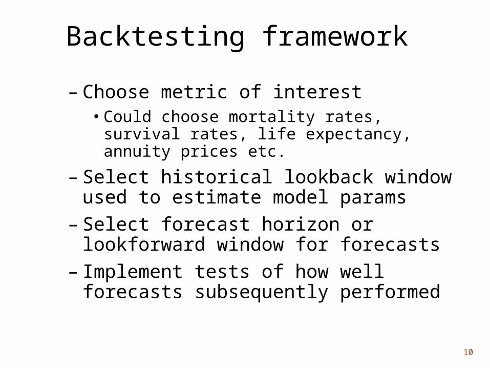
Backtesting framework
– Choose metric of interest• Could choose mortality rates, survival rates, life
expectancy, annuity prices etc.
– Select historical lookback window used to estimate model params
– Select forecast horizon or lookforward window for forecasts
– Implement tests of how well forecasts subsequently performed

11
Backtesting framework
– We choose focus mainly on mortality rate as metric
– We choose a fixed 10-year lookback window• This seems to be emerging as the standard amongst
practitioners
– We examine a range of backtests:• Over contracting horizons
• Over expanding horizons
• Over rolling fixed-length horizons
• Future mortality density tests
12
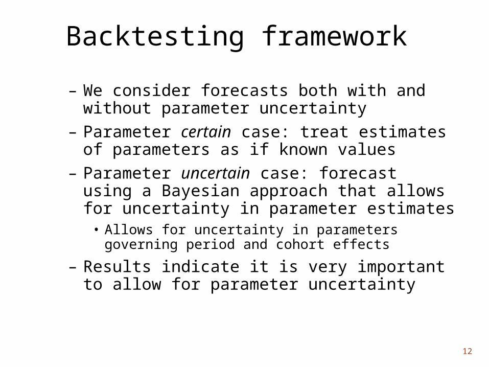
Backtesting framework
– We consider forecasts both with and without parameter uncertainty
– Parameter certain case: treat estimates of parameters as if known values
– Parameter uncertain case: forecast using a Bayesian approach that allows for uncertainty in parameter estimates• Allows for uncertainty in parameters governing period and
cohort effects
– Results indicate it is very important to allow for parameter uncertainty

13
Contracting horizon BT: age 65
1980 1985 1990 1995 2000 20050.01
0.02
0.03
0.04Males aged 65: Model M1
Mor
talit
y ra
te
1980 1985 1990 1995 2000 20050.01
0.02
0.03
0.04Males aged 65: Model M2B
Mor
talit
y ra
te
1980 1985 1990 1995 2000 20050.01
0.02
0.03
0.04Males aged 65: Model M3B
Mor
talit
y ra
te
1980 1985 1990 1995 2000 20050.01
0.02
0.03
0.04Males aged 65: Model M5
Mor
talit
y ra
te
1980 1985 1990 1995 2000 20050.01
0.02
0.03
0.04Males aged 65: Model M6
Stepping off year
Mor
talit
y ra
te
1980 1985 1990 1995 2000 20050.01
0.02
0.03
0.04Males aged 65: Model M7
Stepping off year
Mor
talit
y ra
te

14
Contracting horizon BT: age 75
1980 1985 1990 1995 2000 20050.02
0.04
0.06
0.08
Males aged 75: Model M1
Mo
rtal
ity
rate
1980 1985 1990 1995 2000 20050.02
0.04
0.06
0.08
Males aged 75: Model M2B
Mo
rtal
ity
rate
1980 1985 1990 1995 2000 20050.02
0.04
0.06
0.08
Males aged 75: Model M3B
Mo
rtal
ity
rate
1980 1985 1990 1995 2000 20050.02
0.04
0.06
0.08
Males aged 75: Model M5
Mo
rtal
ity
rate
1980 1985 1990 1995 2000 20050.02
0.04
0.06
0.08
Males aged 75: Model M6
Stepping off year
Mo
rtal
ity
rate
1980 1985 1990 1995 2000 20050.02
0.04
0.06
0.08
Males aged 75: Model M7
Stepping off year
Mo
rtal
ity
rate

15
Contracting horizon BT: age 85
1980 1985 1990 1995 2000 20050.05
0.1
0.15
0.2
0.25Males aged 85: Model M1
Mor
talit
y ra
te
1980 1985 1990 1995 2000 20050.05
0.1
0.15
0.2
0.25Males aged 85: Model M2B
Mor
talit
y ra
te
1980 1985 1990 1995 2000 20050.05
0.1
0.15
0.2
0.25Males aged 85: Model M3B
Mor
talit
y ra
te
1980 1985 1990 1995 2000 20050.05
0.1
0.15
0.2
0.25Males aged 85: Model M5
Mor
talit
y ra
te
1980 1985 1990 1995 2000 20050.05
0.1
0.15
0.2
0.25Males aged 85: Model M6
Stepping off year
Mor
talit
y ra
te
1980 1985 1990 1995 2000 20050.05
0.1
0.15
0.2
0.25Males aged 85: Model M7
Stepping off year
Mor
talit
y ra
te

16
Conclusions so far
• Big difference between PC and PU forecasts
• PU prediction intervals usually considerably wider than PC ones
• M2B sometimes unstable
• Now consider expanding horizon predictions …

17
Prediction-Intervals from 1980: age 65
1980 1985 1990 1995 2000 20050.01
0.02
0.03
0.04
0.05 PC: [xL, xM, xU, n] = [7, 25, 1, 27]
Males aged 65: Model M1
Mo
rtal
ity
rate
PU: [xL, xM, xU, n] = [0, 25, 1, 27]
1980 1985 1990 1995 2000 20050.01
0.02
0.03
0.04
0.05 PC: [xL, xM, xU, n] = [16, 27, 0, 27]
Males aged 65: Model M2B
Mo
rtal
ity
rate
PU: [xL, xM, xU, n] = [8, 27, 0, 27]
1980 1985 1990 1995 2000 20050.01
0.02
0.03
0.04
0.05 PC: [xL, xM, xU, n] = [12, 26, 1, 27]
Mo
rtal
ity
rate
Males aged 65: Model M3B
PU: [xL, xM, xU, n] = [0, 26, 1, 27]
1980 1985 1990 1995 2000 20050.01
0.02
0.03
0.04
0.05 PC: [xL, xM, xU, n] = [18, 27, 0, 27]
Males aged 65: Model M5
Mo
rtal
ity
rate
PU: [xL, xM, xU, n] = [1, 27, 0, 27]
1980 1985 1990 1995 2000 20050.01
0.02
0.03
0.04
0.05
0.06
PC: [xL, xM, xU, n] = [14, 25, 1, 27]
Males aged 65: Model M6
Year
Mo
rtal
ity
rate
PU: [xL, xM, xU, n] = [0, 25, 1, 27]
1980 1985 1990 1995 2000 20050.01
0.02
0.03
0.04
0.05
0.06
PC: [xL, xM, xU, n] = [7, 19, 1, 27]
Year
Mo
rtal
ity
rate
Males aged 65: Model M7
PU: [xL, xM, xU, n] = [0, 19, 1, 27]

18
Prediction-Intervals from 1980: age 75
1980 1985 1990 1995 2000 2005
0.04
0.06
0.08
0.1
PC: [xL, xM, xU, n] = [12, 27, 0, 27]
Males aged 75: Model M1
Mo
rtal
ity
rate
PU: [xL, xM, xU, n] = [1, 27, 0, 27]
1980 1985 1990 1995 2000 2005
0.04
0.06
0.08
0.1
PC: [xL, xM, xU, n] = [13, 27, 0, 27]
Males aged 75: Model M2B
Mo
rtal
ity
rate
PU: [xL, xM, xU, n] = [1, 27, 0, 27]
1980 1985 1990 1995 2000 2005
0.04
0.06
0.08
0.1
PC: [xL, xM, xU, n] = [8, 27, 0, 27]
Mo
rtal
ity
rate
Males aged 75: Model M3B
PU: [xL, xM, xU, n] = [1, 27, 0, 27]
1980 1985 1990 1995 2000 2005
0.04
0.06
0.08
0.1
PC: [xL, xM, xU, n] = [7, 25, 1, 27]
Males aged 75: Model M5
Mo
rtal
ity
rate
PU: [xL, xM, xU, n] = [0, 25, 1, 27]
1980 1985 1990 1995 2000 2005
0.04
0.06
0.08
0.1
PC: [xL, xM, xU, n] = [8, 27, 0, 27]
Males aged 75: Model M6
Year
Mo
rtal
ity
rate
PU: [xL, xM, xU, n] = [1, 27, 0, 27]
1980 1985 1990 1995 2000 2005
0.04
0.06
0.08
0.1
PC: [xL, xM, xU, n] = [9, 27, 0, 27]
Year
Mo
rtal
ity
rate
Males aged 75: Model M7
PU: [xL, xM, xU, n] = [1, 27, 0, 27]
19
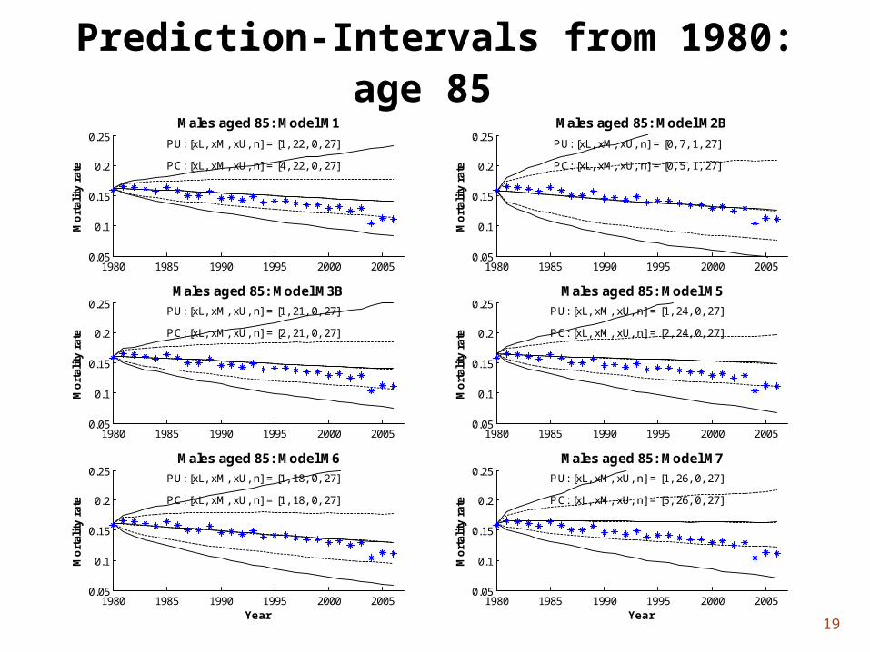
Prediction-Intervals from 1980: age 85
1980 1985 1990 1995 2000 20050.05
0.1
0.15
0.2
0.25
PC: [xL, xM, xU, n] = [4, 22, 0, 27]
Males aged 85: Model M1
Mo
rtal
ity
rate
PU: [xL, xM, xU, n] = [1, 22, 0, 27]
1980 1985 1990 1995 2000 20050.05
0.1
0.15
0.2
0.25
PC: [xL, xM, xU, n] = [0, 5, 1, 27]
Males aged 85: Model M2B
Mo
rtal
ity
rate
PU: [xL, xM, xU, n] = [0, 7, 1, 27]
1980 1985 1990 1995 2000 20050.05
0.1
0.15
0.2
0.25
PC: [xL, xM, xU, n] = [2, 21, 0, 27]
Mo
rtal
ity
rate
Males aged 85: Model M3B
PU: [xL, xM, xU, n] = [1, 21, 0, 27]
1980 1985 1990 1995 2000 20050.05
0.1
0.15
0.2
0.25
PC: [xL, xM, xU, n] = [2, 24, 0, 27]
Males aged 85: Model M5
Mo
rtal
ity
rate
PU: [xL, xM, xU, n] = [1, 24, 0, 27]
1980 1985 1990 1995 2000 20050.05
0.1
0.15
0.2
0.25
PC: [xL, xM, xU, n] = [1, 18, 0, 27]
Males aged 85: Model M6
Year
Mo
rtal
ity
rate
PU: [xL, xM, xU, n] = [1, 18, 0, 27]
1980 1985 1990 1995 2000 20050.05
0.1
0.15
0.2
0.25
PC: [xL, xM, xU, n] = [5, 26, 0, 27]
Year
Mo
rtal
ity
rate
Males aged 85: Model M7
PU: [xL, xM, xU, n] = [1, 26, 0, 27]

20
Expanding PI conclusions
• PC models have far too many lower exceedances
• PU models have exceedances that are much closer to expectations– Especially for M1, M7 and M3B
– Suggests that PU forecasts are more plausible than PC ones
• Negligible differences between PC and PU median predictions
• Very few upper exceedances

21
Expanding PI conclusions
• Too few upper exceedances, and two many median and lower exceedances
• some upward bias, especially for PC forecasts
• This upward bias is especially pronounced for PC forecasts
• Evidence of upward bias less clearcut for PU forecasts

22
Rolling Fixed Horizon Forecasts
• From now on, work with PU forecasts only
• Assume illustrative horizon = 15 years
• Now examine performance of each model in turn …

23
Model M1
1995 1996 1997 1998 1999 2000 2001 2002 2003 2004 2005 200610
-2
10-1
Year
Mo
rtal
ity
rate
Age 65: [xL, xM, xU, n] = [1, 12, 0, 12]
Age 75: [xL, xM, xU, n] = [0, 11, 0, 12]
Age 85: [xL, xM, xU, n] = [1, 10, 0, 12]
Age 65
Age 85
Age 75

24
Model M2B
1995 1996 1997 1998 1999 2000 2001 2002 2003 2004 2005 200610
-2
10-1
Year
Mo
rtal
ity
rate
Age 65: [xL, xM, xU, n] = [8, 12, 0, 12]
Age 75: [xL, xM, xU, n] = [0, 12, 0, 12]
Age 85: [xL, xM, xU, n] = [1, 5, 0, 12]
Age 85
Age 65
Age 75

25
Model M3B
1995 1996 1997 1998 1999 2000 2001 2002 2003 2004 2005 200610
-2
10-1
Year
Mo
rtal
ity
rate
Age 65: [xL, xM, xU, n] = [2, 12, 0, 12]
Age 75: [xL, xM, xU, n] = [0, 12, 0, 12]
Age 85: [xL, xM, xU, n] = [0, 8, 0, 12]
Age 75
Age 65
Age 85

26
Model M5
1995 1996 1997 1998 1999 2000 2001 2002 2003 2004 2005 200610
-2
10-1
Year
Mo
rtal
ity
rate
Age 65: [xL, xM, xU, n] = [9, 12, 0, 12]
Age 75: [xL, xM, xU, n] = [0, 12, 0, 12]
Age 85: [xL, xM, xU, n] = [0, 8, 0, 12]
Age 85
Age 75
Age 65
27
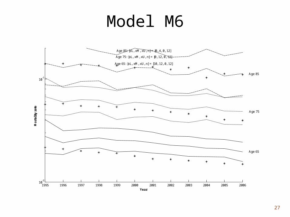
Model M6
1995 1996 1997 1998 1999 2000 2001 2002 2003 2004 2005 200610
-2
10-1
Year
Mo
rtal
ity
rate
Age 65: [xL, xM, xU, n] = [10, 12, 0, 12]
Age 75: [xL, xM, xU, n] = [0, 12, 0, 12]
Age 85: [xL, xM, xU, n] = [0, 4, 0, 12]
Age 85
Age 65
Age 75

28
Model M7
1995 1996 1997 1998 1999 2000 2001 2002 2003 2004 2005 200610
-2
10-1
Year
Mo
rtal
ity
rate
Age 65: [xL, xM, xU, n] = [4, 12, 0, 12]
Age 75: [xL, xM, xU, n] = [0, 12, 0, 12]
Age 85: [xL, xM, xU, n] = [0, 8, 0, 12]
Age 85
Age 75
Age 65

29
Tentative conclusions so far
• Rolling PI charts broadly consistent with earlier results
• Some evidence of upward bias but not consistent across models or always especially compelling
• M2B again shows instability

30
Mortality density tests
• Choose age (e.g., 65) and horizon (e.g., 15 years ahead)
• Use model to project pdf (or cdf) of mortality rate 15 years ahead
• Plot realised q on to pdf/cdf
• Obtain associated p-value (or PIT value)
• Reject if p is too far out in either tail

31
Example: P-Values of Realised Mortality: Males 65, 1980 Start, Horizon = 26 Years Ahead
0 0.005 0.01 0.015 0.02 0.025 0.03 0.035 0.040
0.5
1
CD
F u
nd
er n
ull
Realised q = 0.0149 : p-value = 0.159
Males aged 65: Model M1
0 0.005 0.01 0.015 0.02 0.025 0.03 0.035 0.040
0.5
1
CD
F u
nd
er n
ull
Realised q = 0.0149 : p-value = 0.021
Males aged 65: Model M2B
0 0.005 0.01 0.015 0.02 0.025 0.03 0.035 0.040
0.5
1
CD
F u
nd
er n
ull
Realised q = 0.0149 : p-value = 0.074
Males aged 65: Model M3B
0 0.005 0.01 0.015 0.02 0.025 0.03 0.035 0.040
0.5
1
CD
F u
nd
er n
ull
Realised q = 0.0149 : p-value = 0.049
Males aged 65: Model M5
0 0.005 0.01 0.015 0.02 0.025 0.03 0.035 0.040
0.5
1
Mortality rate
CD
F u
nd
er n
ull
Realised q = 0.0149 : p-value = 0.052
Males aged 65: Model M6
0 0.005 0.01 0.015 0.02 0.025 0.03 0.035 0.040
0.5
1
Mortality rate
CD
F u
nd
er n
ull
Realised q = 0.0149 : p-value = 0.165
Males aged 65: Model M7

32
Many ways to do this
• For h=25 years ahead: 1 way – 1980-2005 only
• For h=24 years ahead, 2 ways– 1980-2004, 1981-2005
• For h=23 years ahead, 3 ways
• ….
• For h=1 year ahead, 26 ways– 1980-1981, 1981-1982, …, 2004-2005

33
Lots of cases to consider
• The are 25+24+23+…+1=325 separate cases to consider, each equally ‘legitimate’
• Need some way to make use of all possibilities but consolidate results
• We do so by computing p-values for each case and then work with mean p-values from each test
• These are reported below for each age, for h=5, 10 and 15 years ahead:

34
Age 65
1985 1990 1995 2000 20050
0.5
1Males aged 65: Model M1
P-v
alu
e
Average = 0.290 for forecasts 5 years aheadAverage = 0.188 for forecasts 10 years aheadAverage = 0.143 for forecasts 15 years ahead
1985 1990 1995 2000 20050
0.5
1Males aged 65: Model M2B
P-v
alu
e
Average = 0.178 for forecasts 5 years aheadAverage = 0.086 for forecasts 10 years aheadAverage = 0.041 for forecasts 15 years ahead
1985 1990 1995 2000 20050
0.5
1Males aged 65: Model M3B
P-v
alu
e
Average = 0.259 for forecasts 5 years ahead
Average = 0.164 for forecasts 10 years aheadAverage = 0.109 for forecasts 15 years ahead
1985 1990 1995 2000 20050
0.5
1Males aged 65: Model M5
P-v
alu
e
Average = 0.107 for forecasts 5 years aheadAverage = 0.063 for forecasts 10 years aheadAverage = 0.042 for forecasts 15 years ahead
1985 1990 1995 2000 20050
0.5
1Males aged 65: Model M6
Starting year
P-v
alu
e
Average = 0.193 for forecasts 5 years aheadAverage = 0.082 for forecasts 10 years aheadAverage = 0.039for forecasts 15 years ahead
1985 1990 1995 2000 20050
0.5
1Males aged 65: Model M7
Starting year
P-v
alu
e
Average = 0.270 for forecasts 5 years aheadAverage = 0.178 for forecasts 10 years aheadAverage = 0.132 for forecasts 15 years ahead

35
Age 75
1985 1990 1995 2000 20050
0.5
1Males aged 75: Model M1
P-v
alu
e
Average = 0.297 for forecasts 5 years aheadAverage = 0.314 for forecasts 10 years aheadAverage = 0.267 for forecasts 15 years ahead
1985 1990 1995 2000 20050
0.5
1Males aged 75: Model M2B
P-v
alu
e
Average = 0.330 for forecasts 5 years aheadAverage = 0.326 for forecasts 10 years aheadAverage = 0.321 for forecasts 15 years ahead
1985 1990 1995 2000 20050
0.5
1Males aged 75: Model M3B
P-v
alu
e
Average = 0.314 for forecasts 5 years aheadAverage = 0.282 for forecasts 10 years aheadAverage = 0.228 for forecasts 15 years ahead
1985 1990 1995 2000 20050
0.5
1Males aged 75: Model M5
P-v
alu
e
Average = 0.308 for forecasts 5 years aheadAverage = 0.291 for forecasts 10 years aheadAverage = 0.228 for forecasts 15 years ahead
1985 1990 1995 2000 20050
0.5
1Males aged 75: Model M6
Starting year
P-v
alu
e
Average = 0.310 for forecasts 5 years aheadAverage = 0.284 for forecasts 10 years aheadAverage = 0.226 for forecasts 15 years ahead
1985 1990 1995 2000 20050
0.5
1Males aged 75: Model M7
Starting year
P-v
alu
e
Average = 0.312 for forecasts 5 years aheadAverage = 0.258 for forecasts 10 years aheadAverage = 0.228 for forecasts 15 years ahead

36
Age 85
1985 1990 1995 2000 20050
0.5
1Males aged 85: Model M1
P-v
alu
e
Average = 0.240 for forecasts 5 years aheadAverage = 0.326 for forecasts 10 years aheadAverage = 0.282 for forecasts 15 years ahead
1985 1990 1995 2000 20050
0.5
1Males aged 85: Model M2B
P-v
alu
e
Average = 0.335 for forecasts 5 years aheadAverage = 0.368 for forecasts 10 years aheadAverage = 0.331 for forecasts 15 years ahead
1985 1990 1995 2000 20050
0.5
1Males aged 85: Model M3B
P-v
alu
e
Average = 0.318 for forecasts 5 years aheadAverage = 0.386 for forecasts 10 years aheadAverage = 0.367 for forecasts 15 years ahead
1985 1990 1995 2000 20050
0.5
1Males aged 85: Model M5
P-v
alu
e
Average = 0.327 for forecasts 5 years aheadAverage = 0.377 for forecasts 10 years aheadAverage = 0.380 for forecasts 15 years ahead
1985 1990 1995 2000 20050
0.5
1Males aged 85: Model M6
Starting year
P-v
alu
e
Average = 0.327 for forecasts 5 years aheadAverage = 0.378 for forecasts 10 years ahead
Average = 0.386 for forecasts 15 years ahead
1985 1990 1995 2000 20050
0.5
1Males aged 85: Model M7
Starting year
P-v
alu
e
Average = 0.330 for forecasts 5 years aheadAverage = 0.370 for forecasts 10 years ahead
Average = 0.371 for forecasts 15 years ahead

37
Conclusions from these tests
• All models perform well
• No rejections at 1% SL
• Only 3 at 5% SL

38
Overall conclusions
• Study outlines a framework for backtesting forecasts of mortality models
• As regards individual models and this dataset:– M1, M3B, M5 and M7 perform well most of the time and there
is little between them
– M2B unstable
– Of the Lee-Carter family of models, hard to choose between M1 and M3B
– Of the CBD family, M7 seems to perform best; little to choose between M5 and M7
39
Two other points stand out
• In many but not all cases, and depending also on the model, there is evidence of an upward bias in forecasts– This is very pronounced for PC forecasts
– This bias is less pronounced for PU forecasts
• Except maybe for M2B, PU forecasts are more plausible than the PC forecasts
• Very important to take account of param uncertainty more or less regardless of the model one uses

40
References
• Cairns et al. (2007) “A quantitative comparison of stochastic mortality models using data from England & Wales and the United States.” Pensions Institute Discussion Paper PI-0701, March
• Cairns et al. (2008) “The plausibility of mortality density forecasts: An analysis of six stochastic mortality models.” Pensions Institute Discussion Paper PI-0801, April.
• Dowd et al. (2008a) “Evaluating the goodness of fit of stochastic mortality models.” Pensions Institute Discussion Paper PI-0802, September.
• Dowd et al. (2008b) “Backtesting stochastic mortality models: An ex-post evaluation of multi-year-ahead density forecasts.” Pensions Institute Discussion Paper PI-0803, September.
• These papers are also available at www.lifemetrics.com