Back to pink ?

MMM Moving Mic Measurement, part 1A method for spatial averaging of loudspeakers in-room measurements

This presentation of MMM, Moving Mic Measurement, begins with an explanation of why loudspeaker/room equalization is not valid when based on a measurement done at a single point and why spatial averaging of multiple points measurements is mandatory.In the second part, the Moving Mic Measurement is presented, which is as precise but much quicker than standard multiple points measurements.Caution notes : this study is only related to music at home, home theaters, mixing and screening rooms, music studios,... but not for PA, line-arrays,... MMM has one purpose : in-room measurements of final product for equalization purposes. It is not a tool for R&D of loudspeakers boxes, crossovers, positions, diffraction, time-alignement,….

www.abayx.com www.ohl.to Jean-Luc Ohl, v1.7, dec 2014

First, let's look at some measurements :hereunder are measurements at 9 positions separated by about 10cm in a cinema mixing room build with serious acoustic treatments (200m3, RT of 0.2s at 500Hz, MeyerSound EXP system measured before any EQ). It shows variations up to 16dB from 0.5 to 2kHz, a very sensible zone, (amplitude obtained from impulse response measured with log sinesweep).

Picture 1

Graph of differences between positions :

Picture 2

In this room, the spectral balance and timbral quality are similary perceived for all positions near central listening position*1 despite measurements showing large differences. This is a allways the case : in cinema mixing rooms, music studios,... measured differences between nearby positions are important even without any perceived difference. There is no correlation between measurements and listening quality. We think that the subjective quality should command the measuring method : one has to measure and correct what is really perceived, not more not less. This paper presents a method better related to perceived audio quality.

www.abayx.com www.ohl.to Jean-Luc Ohl, v1.7, dec 2014

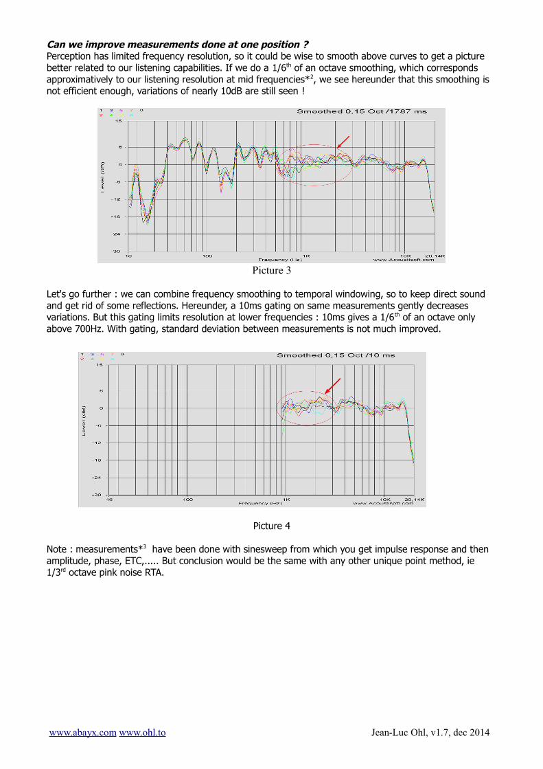
Can we improve measurements done at one position ?Perception has limited frequency resolution, so it could be wise to smooth above curves to get a picture better related to our listening capabilities. If we do a 1/6th of an octave smoothing, which corresponds approximatively to our listening resolution at mid frequencies*2, we see hereunder that this smoothing is not efficient enough, variations of nearly 10dB are still seen !

Picture 3

Let's go further : we can combine frequency smoothing to temporal windowing, so to keep direct sound and get rid of some reflections. Hereunder, a 10ms gating on same measurements gently decreases variations. But this gating limits resolution at lower frequencies : 10ms gives a 1/6th of an octave only above 700Hz. With gating, standard deviation between measurements is not much improved.

Picture 4

Note : measurements*3 have been done with sinesweep from which you get impulse response and then amplitude, phase, ETC,..... But conclusion would be the same with any other unique point method, ie 1/3rd octave pink noise RTA.

www.abayx.com www.ohl.to Jean-Luc Ohl, v1.7, dec 2014

And why not use a frequency dependent time window ? On the same measurements as above, let's try an adaptative window of 6 periods to avoid reflections as much as possible (HOLM permits to show only three simultaneous curves so some of the most different responses have been choosen).

In mid frequencies, the variance on amplitude is still important.Let's check another example of measurements done in a cube of 40cm at main listening position of a mixing stage (X curve equalized)

In both examples, we clearly see that we cannot rely on a frequency dependent window to EQ.

It seems that classical measurements at one position cannot be representative of perceived quality : those measurements are too dependant of exact measuring position or small changes of environnement (ie wind, temperature),... Signal processing (smoothing, gating fixed or variable) do not lessen variance. Measurement at one point being neither accurate nor reproductible, you simply cannot use it for precise equalization.Let's give the last word to Floyd Toole : « spatial-averaging of speaker measurements is criti-cal —single-point measurements are erroneous and meaningless »

www.abayx.com www.ohl.to Jean-Luc Ohl, v1.7, dec 2014

If a single point method cannot be efficient, are there other solutions ?If quality is the same for nearby listening places, let's check common factors. For measurements to be independant (this can be checked by crosscorrelation), they have to be done at random places far enough from each other, more than a half wavelength, and at different coordinates (in length, width and heigth) but within a directivity cone of about 15° from loudspeaker axis. Here is a set of 32 measurements : we see that above 300Hz, curves stay within +-6dB.

Picture 5We have to check if those measurements are repeatable and so independant of exact measuring position : we separate the whole set into two groups and start with the 16 odd measurements (n°1,3,5,...).

Picture 6

Now the 16 even measurements (n°2,4,6,...)

Picture 7

www.abayx.com www.ohl.to Jean-Luc Ohl, v1.7, dec 2014

Let's now have a look to amplitude averages.

Average of all 32 measurements

Picture 8

Average of the 16 odd measurements

Picture 9

Average of the 16 even measurements

Picture 10

Separating in two groups, we see that averages are all very near with less than 2dB differences above 200Hz. Even with this minimal smoothing, this is a good indicator for reproductibility.

www.abayx.com www.ohl.to Jean-Luc Ohl, v1.7, dec 2014

Can we explain above results with a few acoustics ?

In the diffuse field, far enough from sources, direct sound and wall reflections combine and create comb filtering effects that vary depending on the exact position and this is seen on above curves. Acousticians separate the audible frequency range in two zones :

Under the transition frequency Tf (also called Schroeder frequency), acoustic is more deterministic : it is modal zone with modes depending on room dimensions. Those modes are clearly seen on unsmoothed curves.

Above that range, acoustic is more chaotic, modes are too numerous and the acoustic field is modified by every surface. Acoustic pressure at one point is better seen as a statistical variable. Schroeder*4 and Geddes*5 have calculated with different methods the standard deviation on amplitude and have found similar results : the standard deviation is about +-5.57dB with 70% confidence. If we prefer to work with 95% confidence, the standard deviation of a Gaussian statistical curve is nearly two times more, so it gives a standard deviation of σ = 2*5.57/√(1+2.38*B*Tr)*16, with B bandwidth and Rt reverberation time.

Note : that transition frequency goes from about 40Hz for a cinema to 300Hz for a small room. We generally speak of a frequency but it would be more acurate to speak of a frequency range.At 1000Hz and for a 0.3s Rt, we get following deviations :

without smoothing : +-11.1dB1/48th octave smoothing : +-7.1dB1/20th octave smoothing : +-5.2dB1/6th octave smoothing : +-3.3dB1/3th octave smoothing : +-2.2dB

We seen above that for a unique point measurement, 1/6th octave smoothing and short gating improves variance but not enough for a precise correction. Measuring at different places far from loudspeakers, effects of random reflections will average. But the loudspeaker direct field, near walls (room gain) and diffraction effects are not random so won't disappear from averaging and will be accounted in the averaged curve. Another way to keep direct field and lower reflections, would be to use microphones with some directivity.

Our hearing model works on same principle : due to time integration of the inner ear, first reflections are merged with direct sound and influence timbre, later arrivals are perceived separately and do not change source timbre.

www.abayx.com www.ohl.to Jean-Luc Ohl, v1.7, dec 2014

How precise should be the measurement : audibility of spectral deviations

Speaking of frequency response, the estimation of audible deviation from an ideal curve*6*7, is about 2 dB on ERB scale*8 (near 1/6th octave at mid frequencies). So it should be necessary to EQ better than +-1dB at mid frequencies and for this, it is mandatory to measure with same or better resolution.For random reflections, standard deviation is related to square root of measurement number*9 N : σ = 11.14/(√(1+2.38*B*Tr)*√N)

at 1000Hz and a smoothing of 1/6th octave, we need 10 independant measurements (3.3/√10 =1dB) to stay within +-1dB. As independant measurements have to be separated of more than 1/4th of wavelength, this gives a measuring distance of 1m

at 100Hz, perception is less performant : acceptable deviation is higher and ERB bandwidth is about 0.35 octave, we need 9 independant measurements (6/√9=2dB) to stay within +-2dB. This gives a measuring distance of about 8m.

For multiple positions on a measured length L, σ = 11.14/√((1+0,238*B*Tr)*L*4*F/c)with B bandwith in Hz, Tr reverberation time in s, L measuring distance in m, F frequency in Hz, c sound celerity in m/s.

For same deviation at lower frequencies, longer measuring distances are needed, see picture 11.But remember that those curves are based on statistical acoustics so are only valid above half transition frequency*16.

Picture 11

We see that longer distances average better, but how much should we average lower frequencies in rooms where a main listening position is defined ? Ie if one tries to scan over too large a volume, some low frequency modes may be averaged out.

www.abayx.com www.ohl.to Jean-Luc Ohl, v1.7, dec 2014

20 40 80 160 315 630 1250 2500 5000 10000 200000,10

1,00

10,00

with 1/6th octave resolution

2010521

stan

dard

dev

iatio

n dB

Standard deviation / measuring distance (m)

distance (m)

20 40 80 160 315 630 1250 2500 5000 10000 200000,10

1,00

10,00

with ERB resolution

2010521

stan

dard

dev

iatio

n dB

Standard deviation / measuring distance (m)

distance (m)

MMM Moving Mic Measurement : another way for spatial averaging

Can we learn from field sound insulation testing ? Standards have been revised recently*11 : Technical reasons : National Building Regulations require repeatable and reproducible

measurements To allow quick measurements on noisy building sites, acoustic consultants were interested in using

manual scanning in an engineering method : to reduce the equipment and cabling that is needed for field measurements, to reduce measurement times,...

That's also what is asked for loudspeaker measurements !

So instead of multiple points measurements, we can also use MMM, a Moving Mic Measurement. We need a continuous signal, pink noise is the ideal candidate. MLS is not recommended and sinesweeps are not adapted. So with long time scanning, FFT analysis and rms averaging, the method combines temporal and spatial averaging. But note that the averaging has to be done on the whole scan duration, not a gliding average, with some constraints on calculation.

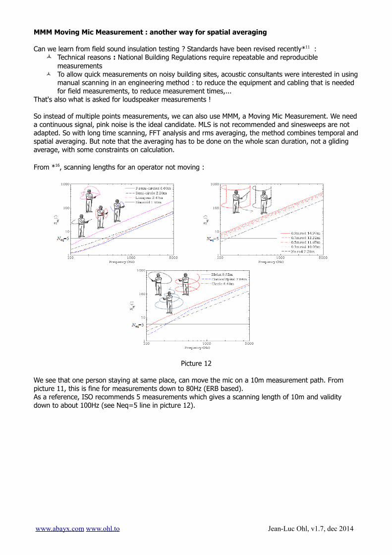
From *16, scanning lengths for an operator not moving :

Picture 12

We see that one person staying at same place, can move the mic on a 10m measurement path. From picture 11, this is fine for measurements down to 80Hz (ERB based).As a reference, ISO recommends 5 measurements which gives a scanning length of 10m and validity down to about 100Hz (see Neq=5 line in picture 12).

www.abayx.com www.ohl.to Jean-Luc Ohl, v1.7, dec 2014

Measuring distance, standard deviation and perception

I tried to check the relation between measuring distance, number of independant measuring points, resulting standard deviation and perception, to evaluate what is the needed scanning distance :

The relation between measuring distance and number of independant measuring points comes from Hopkins12.

The standard deviation is calculated from number of points based on equation σ = 11.14/(√(1+2.38*B*Tr)*√N), from Schroeder4 and Hopkins16

The approximate frequency dependant threshold of perception is an estimation based on Moore2, Clark (see picture) and Toole6 and some personnal ABX listening tests. This curve should correspond to the threshold of audibility of 1/6th octave bandwidth deviations on a signal, with pink noise generally being the most revealing signal.

Picture 13Clark, David, "High-Resolution Subjective Testing Using a Double-Blind Comparator", AES may 1982« Each curve indicates the smallest amount of amplitude difference at each frequency that has been

heard in ABX tests, when the bandwidth of the difference is about that of the curve's name »

Clark's picture only shows 1/3 oct bandwidth but I used same values in the graphic hereunder (!), this may be a bit conservative. This perception curve can be seen as a peak to mid value : the level difference between a peak and the flat curve.

Thanks to above calculations, we can now check which scanning length is needed : it seems that a scanning of 5m gives statistical deviations low enough to match « just noticeable perception ».

Picture 14

www.abayx.com www.ohl.to Jean-Luc Ohl, v1.7, dec 2014

Accurate measurements

Acoustic measurement for equalizing has to be validated from sound perception but has to be based on standard metrology criterias :

resolution uncertainty which depends on two criterias : precision asked for repeatable measurements and

accuracy needed to minimize systematic errors.

We have seen above that measuring at one position does not give repeatable measurements and has not good enough resolution.

MMM is quick and and efficient for equalization of a loudspeakers but because it is missing the time and phase information, it is not a tool to set up crossovers, time align speakers,...(for this, you need first an MLS or sinesweep measurement at one point).There are some constraints to get reliable measurements with MMM :

Calibration : the pink noise has to be checked for its frequency response and microphone should be calibrated for random incidence diffuse field.

Measurement must average on enough independant positions : so move microphone to cover a volume large enough : a 5m scanning distance is a good basis (ie 3 semi-circles). Another way is to cover a volume with dimensions of about 1/5th of corresponding room dimension, it has beeen tested to give reliable results down to Tf.

Measurements should avoid systematic errors, ie not all measurements at same height ! Do traverse movements, more than 10 degrees from any plane of the room*14

Do not move mic too close to boundaries (min 1m recommended) Do not move too fast (max 0.3m/s), there should be no risk of Doppler distortion*15 but more risk

of wind or operator noise. Also use non-microphonic cables. Mic shall not be pointed directly to loudspeaker : due to semi-diffuse field, microphone can be

pointed randomly during scanning or kept at 90° from source (grazing incidence), both techniques give near results with small mics (1/4" or less) but allways keep microphone in direct view of loudspeaker.

Averaging is to be done on mean-squared sound pressures and on a long enough time : no short average or moving average. An average on a whole sequence of 30s seems to give good resolution and reproductibility (ISO/WD 16283-1 recommends 60s for frequencies under 100Hz*11)

Measurement has to be better than our hearing resolution : use a 1/6th frequency octave smoothing or less.

Fullfilling those conditions, MMM will give excellent reproductibility. Good stability of results with time is expected, contrary to unique point measurement where response changes are often said to come from loudspeakers aging when in reality it is just because of poor measurements repeatability !The resulting MMM measured response shows 3 of the 4 main parameters caracterized by Olive

as beeing

the most relevant to perceived sound quality : Narrow Band Deviation in room NBD_PIR, Low frequency extension LFX , Smoothness in amplitude response in room SM_PIR. All those curves can be seen on MMM measurements. Narrow Band Deviation NBD_ON on axis is missing but isn't it related to Narrow Band Deviation in room ?

It is encouraging to find that stereo and multichannel systems, measured and corrected with MMM, show excellent timbre matching between loudspeakers, this can be checked by switching between channels while listening to pink noise, the most revealing signal for this test. This is a good indicator and correlation between MMM measurement method and auditive perception will be studied in a next paper.

To ease MMM measurements, ABAYX is using its own software. This software will also be available to other companies beginning of 2015.

www.abayx.com www.ohl.to Jean-Luc Ohl, v1.7, dec 2014

Notes and references*1 Here we strictly speak of timbral accuracy and not of localisation accuracy for which exact position can be important.*2 The ear resolution is about 0.15 octave at mid frequencies, as per cochlear model and ERB (Equivalent Rectangular Bandwidth) curves from Moore, B.C.J., An Introduction to the Psychology of Hearing.*3 Acoustisoft R+D by Doug Plumb : the very interesting manual of a recommended software. *4 Schroeder M.R., Statistical parameters of the frequency response curves of large rooms.*5 Geddes E., Audio transducers.*6 Toole F.O., Sound reproduction, loudspeakers and rooms.*7 Olive S., A Multiple Regression Model for Predicting Loudspeaker Preference Using Objective Measurements.*8 With gammatone filters, simulated by parallel filters with a Q of 7, just noticeable amplitude difference is about 2dB.*9 Geddes E., Blind H., The localized sound power method, AES journal vol.34, march 1986.*11 Standard ISO/FDIS 16283-1:2013 Acoustics - Field measurement of sound insulation in buildings and of building elements*12 Hopkins C., On the efficacy of spatial sampling using manual scanning paths to determine the spatial average sound pressure level in rooms. Journal of the Acoustical Society of America vol 129 issue 5, 2011. *13 Simmons C., Uncertainties of room average sound pressure levels measured in the field according to the draft standard ISO 16283-1*14ANC Schools Good Practice Guide 110711*15 Ajdler, T. et al, Room impulse responses measurement using a moving microphone, Presented at the 120th AES Convention 2006 May 20–23.*16 Hopkins C., Sound Insulation, BH 2007.*17 Critchley I., Dunbavin.P., An empirical study of the effects of occupied test rooms and a moving microphone when measuring Airborne Sound Insulation, IOA Spring Conference 2008.

www.abayx.com www.ohl.to Jean-Luc Ohl, v1.7, dec 2014

Annex 1 Comparison with another multiple points method

Dirac 15 positions averagedDifference at higher frequencies may be explained by mic calibration for Dirac : Earthworks mic is calibrated at 0° and used at 90° !

MMM around main listening position

Annex 2 Comparison with anechoic measurements

a2 Sean Olive (Harman) published measurements on Infinity Primus P3604 curves : on axis, direct sound, with first reflections, power response

a3 Comparison between Harman's results and P360 in a living room :above 150-200Hz, MMM curve is between « direct sound » and « first reflections »

3 different random movements of 30s each, in same zone : repeatability is very good.

www.abayx.com www.ohl.to Jean-Luc Ohl, v1.7, dec 2014

Annex 3Various measurements

a4 Comparison in same room between L and R with moving mic method. Despite asymetric positions of the speakers, MMM shows similar curves.

a5 Same comparison between L and R but measured at one point. The differences between channels are important, much more than with MMM averaging.

a6 Same comparison at only one position but with 1/3rd octave smoothing.The differences between channels are important and Eq based on those responses would be very different from one based on a4

www.abayx.com www.ohl.to Jean-Luc Ohl, v1.7, dec 2014

Annex4Is MMM a power response measurement ?

In a standard living room (5.4x4.5x2.8m) with no acoustic treatments, we have measured with MMM at 0.5, 1, 2 and 3m and plot the difference. At 3m, beyond critical distance, the attenuation at 15kHz is only about 3dB, very far from power response DI (about 10dB for those loudspeakers, see a3) and even less than first reflections DI (5dB).

a7 : b2030 difference plot between 0.5m and 1,2 and 3m.at 15kHz and 3m, attenuation is 2.8dB compared to 0.5m.

A8 : p360 difference plot between 0.5m and 1,2 and 3m.At 15kHz and 3m, attenuation is 3.1dB compared to 0.5m.

In those conditions, it is clear that MMM is not a power response measurement. Comparing to picture a2, it is quite near from a PIR or First Reflections measurement.

www.abayx.com www.ohl.to Jean-Luc Ohl, v1.7, dec 2014

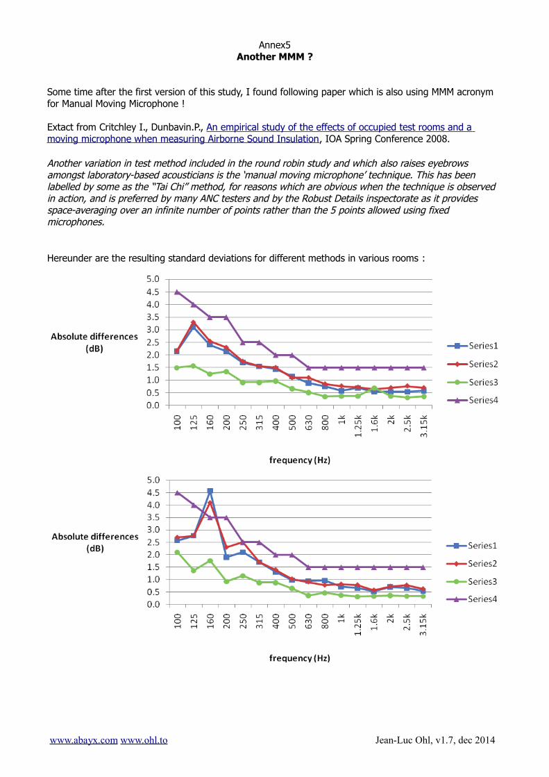
Annex5Another MMM ?

Some time after the first version of this study, I found following paper which is also using MMM acronym for Manual Moving Microphone !

Extact from Critchley I., Dunbavin.P., An empirical study of the effects of occupied test rooms and a moving microphone when measuring Airborne Sound Insulation, IOA Spring Conference 2008.

Another variation in test method included in the round robin study and which also raises eyebrows amongst laboratory-based acousticians is the ‘manual moving microphone’ technique. This has been labelled by some as the “Tai Chi” method, for reasons which are obvious when the technique is observed in action, and is preferred by many ANC testers and by the Robust Details inspectorate as it provides space-averaging over an infinite number of points rather than the 5 points allowed using fixed microphones.

Hereunder are the resulting standard deviations for different methods in various rooms :

www.abayx.com www.ohl.to Jean-Luc Ohl, v1.7, dec 2014

Series 1 -Static microphone, unoccupied roomsSeries 2 -Static microphone, Source room unoccupied when receiver room occupiedSeries 3 -Moving microphoneSeries 4 - ISO 140-2:1991

www.abayx.com www.ohl.to Jean-Luc Ohl, v1.7, dec 2014

So I reported above results from Critchley & Dunbavin study into my own plots, modified to 1/3rd octave resolution and 1s RT, it gives following curve, in red. This resulting standard deviation ASI curve (Airborne Sound Insulation) agrees well with a theoretical scan between 5 and 10m.

One conclusion of the Critchley & Dunbavin round-robin test is : 8. This investigation suggests that the manual moving mic technique (MMM) […] produces the most repeatable results in rooms of 30m3 or more when compared with any of the other test methods. Most notable is the improved accuracy and repeatability of this method at low frequency, where modal variations produce well-documented inaccuracies in the other, more traditional test methods.

www.abayx.com www.ohl.to Jean-Luc Ohl, v1.7, dec 2014

20 40 80 160 315 630 1250 2500 5000 10000 200001

10

100

1000

IOA airborne sound insulation fig 25, 26, 35 and 36, 1/3oct smoothing, Rt 1s

0.25dB0.5dB1dB2dB10m scan5m scan2m scanASI

standarddeviation dB

measurementsnr