Bachman d. a_geometric_approach_to_differential_forms__2012
173
-
Upload
david-quintero -
Category
Technology
-
view
324 -
download
6
description
Geometria diferencial
Transcript of Bachman d. a_geometric_approach_to_differential_forms__2012

David Bachman
A Geometric Approachto Differential Forms
Second Edition
ISBN 978-0-8176-8303-0 e-ISBN 978-0-8176-830 -DOI 10.1007/978-0-8176-830 -
Library of Congress Control Number:
Mathematics Subject Classification (2010
Springer New York Dordrecht Heidelberg London
4 74 7
): 53-01, 53A04, 53A05, 53A45, 53B21, 58A10, 58A12, 58A15
2011940222
David Bachman
Department of Mathematics1050 N. Mills AvenueClaremont, CA 91711
Pitzer College
© Springer Science+Business Media, LLC 2006, 2012
Printed on acid-free paper
All rights reserved. This work may not be translated or copied in whole or in part without the written permission of the publisher (Birkhäuser Boston, c/o Springer Science+Business Media, LLC, 233 Spring Street, New York, NY 10013, USA), except for brief excerpts in connection with reviews or scholarly analysis. Use in connection with any form of information storage and retrieval, electronic adaptation, computer software, or by similar or dissimilar methodology now known or hereafter developed is forbidden. The use in this publication of trade names, trademarks, service marks, and similar terms, even if they are not identified as such, is not to be taken as an expression of opinion as to whether or not they are subject to proprietary rights.
Birkhäuser Boston is part of Springer Science+Business Media (www.birkhauser.com)
Preface to the Second Edition
The original edition of this book was written to be accessible to sophomore-level undergraduates, who had only seen one year of a standard calculus se-quence. In particular, for most of the text, no prior exposure to multivariablecalculus, vector calculus, or linear algebra was assumed. After receiving lotsof reader feedback to the first edition, it became clear that the people readingthis book were more advanced. Hence, for the second edition, most of thematerial on basic topics such as partial derivatives and multiple integrals hasbeen removed, and more advanced applications of differential forms have beenadded.
The largest of the new additions is a chapter containing an introductionto differential geometry, based on the machinery of differential forms. At alltimes, we have made an effort to be consistent with the rest of the text here,so that the material is presented in R
3 for concreteness, but all definitionsare formulated to easily generalize to arbitrary dimensions. This is perhaps aunique approach to this material.
Other smaller additions worth noting include new sections on linkingnumber and the Hopf Invariant. These join the host of brief applicationsof differential forms which originally appeared in the first edition, includingMaxwell’s Equations, DeRham Cohomology, foliations, contact structures, andthe Godbillon–Vey Invariant. While the treatment given here of these topicsis far from exhaustive, we feel it is important to include these teasers to givethe reader some hint at the usefulness of differential forms.
Finally, other changes worth noting are a rearrangement of some of theoriginal sections for clarity, and the addition of several new problems andexamples.
Claremont, CA David BachmanJanuary, 2011
v

Preface to the First Edition1
The present work is not meant to contain any new material about differentialforms. There are many good books out there which give complete treatmentsof the subject. Rather, the goal here is to make the topic of differential formsaccessible to the sophomore-level undergraduate while still providing materialthat will be of interest to more advanced students.
There are three tracks through this text. The first is a course in Multivari-able Calculus, suitable for the third semester in a standard calculus sequence.The second track is a sophomore-level Vector Calculus class. The last track isfor advanced undergraduates, or even beginning graduate students. At manyinstitutions, a course in linear algebra is not a prerequisite for either multi-variable calculus or vector calculus. Consequently, this book has been writtenso that the earlier chapters do not require many concepts from linear algebra.What little is needed is covered in the first section.
The book begins with basic concepts from multivariable calculus such aspartial derivatives, gradients and multiple integrals. All of these topics areintroduced in an informal, pictorial way to quickly get students to the pointwhere they can do basic calculations and understand what they mean. Thesecond chapter focuses on parameterizations of curves, surfaces and three-dimensional regions. We spend considerable time here developing tools whichwill help students find parameterizations on their own, as this is a commonstumbling block.
Chapter 1 is purely motivational. It is included to help students understandwhy differential forms arise naturally when integrating over parameterizeddomains.
The heart of this text is Chapters 3 through 6. In these chapters, the entiremachinery of differential forms is developed from a geometric standpoint. Newideas are always introduced with a picture. Verbal descriptions of geometricactions are set out in boxes.
1 Chapter and Section references have been updated to conform to the presentedition.
vii
Chapter 6 focuses on the development of the generalized Stokes’ Theo-rem. This is really the centerpiece of the text. Everything that precedes it isthere for the sole purpose of its development. Everything that follows is anapplication. The equation is simple:∫
∂C
ω =
∫C
dω.
Yet it implies, for example, all integral theorems of classical vector analysis.Its simplicity is precisely why it is easier for students to understand andremember than these classical results.
Chapter 6 concludes with a discussion on how to recover all of vector cal-culus from the generalized Stokes’ Theorem. By the time students get throughthis they tend to be more proficient at vector integration than after traditionalclasses in vector calculus. Perhaps this will allay some of the concerns manywill have in adopting this textbook for traditional classes.
Chapter ∗∗2 contains further applications of differential forms. These in-clude Maxwell’s Equations and an introduction to the theory of foliationsand contact structures. This material should be accessible to anyone who hasworked through Chapter 6.
Chapter 7 is intended for advanced undergraduate and beginning graduatestudents. It focuses on generalizing the theory of differential forms to thesetting of abstract manifolds. The final section contains a brief introductionto DeRham Cohomology.
We now describe the three primary tracks through this text.
Track 1. Multivariable Calculus (Calculus III).3 For such a course, oneshould focus on the definitions of n-forms on R
m, where n and m are at most3. The following chapters/sections are suggested:
• Chapter 2, perhaps supplementing Section 2.2 with additional material onmax/min problems,
• Chapter ∗∗4,• Chapter 3, excluding Sections 3.4 and 3.5 due to time constraints,• Chapters 4–6,5
• Appendix A.6
Track 2. Vector Calculus. In this course, one should mention that for n-forms on R
m, the numbers n and m could be anything, although in practice
2 This material has been added to the end of Chapter 5 in the present edition.3 The present edition may not be quite as suitable for such a course as the firstedition was.
4 Material has been removed in the present edition.5 The material in Sections 5.6, 5.7 and 6.4 were not originally included in thesechapters.
6 This is now Section 4.8.
viii Preface
Preface to the First Edition
it is difficult to work examples when either is bigger than 4. The followingchapters/sections are suggested:
• Section ∗∗ (unless Linear Algebra is a prerequisite),7
• Chapter 1 (one lecture),• Chapter 2,• Chapters 3–6,• Sections 6.4 through 5.7, as time permits.
Track 3. Upper Division Course. Students should have had linear algebra,and perhaps even basic courses in group theory and topology.
• Chapter 1 (perhaps as a reading assignment),• Chapters 3–6 (relatively quickly),• Sections 6.4 through 5.7 and Chapter 7.
The original motivation for this book came from [GP10], the text I learneddifferential topology from as a graduate student. In that text, differential formsare defined in a highly algebraic manner, which left me craving somethingmore intuitiuve. In searching for a more geometric interpretation I came acrossChapter 7 of Arnold’s text on classical mechanics [Arn97], where there is awonderful introduction to differential forms given from a geometric viewpoint.In some sense, the present work is an expansion of the presentation given there.Hubbard and Hubbard’s text [HH99] was also a helpful reference during thepreparation of this manuscript.
The writing of this book began with a set of lecture notes from an intro-ductory course on differential forms, given at Portland State University, dur-ing the summer of 2000. The notes were then revised for subsequent courseson multivariable calculus and vector calculus at California Polytechnic StateUniversity, San Luis Obispo and Pitzer College.
I thank several people. First and foremost, I am grateful to all those stu-dents who survived the earlier versions of this book. I would also like to thankseveral of my colleagues for giving me helpful comments. Most notably, DonHartig, Matthew White and Jim Hoste had several comments after using ear-lier versions of this text for vector or multivariable calculus courses. JohnEtnyre and Danny Calegari gave me feedback regarding Section 5.6 and SaulSchleimer suggested Example 27. Other helpful suggestions were provided byRyan Derby–Talbot. Alvin Bachman suggested some of the formatting of thetext. Finally, the idea to write this text came from conversations with RobertGhrist while I was a graduate student at the University of Texas at Austin.
Claremont, CA David BachmanMarch, 2006
7 Material has been removed in the present edition.
ix

Contents
Preface to the Second Edition . . . . . . . . . . . . . . . . . . . . . . . . . . . . . . . . . v
Preface to the First Edition . . . . . . . . . . . . . . . . . . . . . . . . . . . . . . . . . . . vii
Guide to the Reader . . . . . . . . . . . . . . . . . . . . . . . . . . . . . . . . . . . . . . . . . . . xv
1 Introduction . . . . . . . . . . . . . . . . . . . . . . . . . . . . . . . . . . . . . . . . . . . . . . . 11.1 So what is a differential form? . . . . . . . . . . . . . . . . . . . . . . . . . . . . 11.2 Generalizing the integral . . . . . . . . . . . . . . . . . . . . . . . . . . . . . . . . . 21.3 What went wrong? . . . . . . . . . . . . . . . . . . . . . . . . . . . . . . . . . . . . . . 31.4 What about surfaces? . . . . . . . . . . . . . . . . . . . . . . . . . . . . . . . . . . . . 5
2 Prerequisites . . . . . . . . . . . . . . . . . . . . . . . . . . . . . . . . . . . . . . . . . . . . . . 72.1 Multivariable calculus . . . . . . . . . . . . . . . . . . . . . . . . . . . . . . . . . . . . 72.2 Gradients . . . . . . . . . . . . . . . . . . . . . . . . . . . . . . . . . . . . . . . . . . . . . . 102.3 Polar, cylindrical and spherical coordinates . . . . . . . . . . . . . . . . . 142.4 Parameterized curves . . . . . . . . . . . . . . . . . . . . . . . . . . . . . . . . . . . . 162.5 Parameterized surfaces in R
3 . . . . . . . . . . . . . . . . . . . . . . . . . . . . . . 192.6 Parameterized regions in R
2 and R3 . . . . . . . . . . . . . . . . . . . . . . . 21
3 Forms . . . . . . . . . . . . . . . . . . . . . . . . . . . . . . . . . . . . . . . . . . . . . . . . . . . . . 253.1 Coordinates for vectors . . . . . . . . . . . . . . . . . . . . . . . . . . . . . . . . . . . 253.2 1-Forms . . . . . . . . . . . . . . . . . . . . . . . . . . . . . . . . . . . . . . . . . . . . . . . . 273.3 Multiplying 1-forms . . . . . . . . . . . . . . . . . . . . . . . . . . . . . . . . . . . . . . 293.4 2-Forms on TpR
3 (optional) . . . . . . . . . . . . . . . . . . . . . . . . . . . . . . . 343.5 2-Forms and 3-forms on TpR
4 (optional) . . . . . . . . . . . . . . . . . . . . 363.6 n-Forms . . . . . . . . . . . . . . . . . . . . . . . . . . . . . . . . . . . . . . . . . . . . . . . . 373.7 Algebraic computation of products . . . . . . . . . . . . . . . . . . . . . . . . 40
xi
Contents
4 Differential Forms . . . . . . . . . . . . . . . . . . . . . . . . . . . . . . . . . . . . . . . . . 414.1 Families of forms . . . . . . . . . . . . . . . . . . . . . . . . . . . . . . . . . . . . . . . . 414.2 Integrating differential 2-forms . . . . . . . . . . . . . . . . . . . . . . . . . . . . 434.3 Orientations . . . . . . . . . . . . . . . . . . . . . . . . . . . . . . . . . . . . . . . . . . . . 504.4 Integrating 1-forms on R
m . . . . . . . . . . . . . . . . . . . . . . . . . . . . . . . . 534.5 Integrating n-forms on R
m . . . . . . . . . . . . . . . . . . . . . . . . . . . . . . . . 554.6 The change of variables formula . . . . . . . . . . . . . . . . . . . . . . . . . . . 57
4.6.1 1-Forms on R1 . . . . . . . . . . . . . . . . . . . . . . . . . . . . . . . . . . . . 57
4.6.2 2-Forms on R2 . . . . . . . . . . . . . . . . . . . . . . . . . . . . . . . . . . . . 58
4.6.3 3-Forms on R3 . . . . . . . . . . . . . . . . . . . . . . . . . . . . . . . . . . . . 62
4.7 Summary: How to integrate a differential form . . . . . . . . . . . . . . 644.7.1 The steps . . . . . . . . . . . . . . . . . . . . . . . . . . . . . . . . . . . . . . . . 644.7.2 Integrating 2-forms . . . . . . . . . . . . . . . . . . . . . . . . . . . . . . . . 654.7.3 A sample 2-form . . . . . . . . . . . . . . . . . . . . . . . . . . . . . . . . . . 66
4.8 Nonlinear forms (optional) . . . . . . . . . . . . . . . . . . . . . . . . . . . . . . . . 674.8.1 Surface area . . . . . . . . . . . . . . . . . . . . . . . . . . . . . . . . . . . . . . 674.8.2 Arc length . . . . . . . . . . . . . . . . . . . . . . . . . . . . . . . . . . . . . . . . 69
5 Differentiation of Differential Forms . . . . . . . . . . . . . . . . . . . . . . . 715.1 The derivative of a differential 1-form . . . . . . . . . . . . . . . . . . . . . . 715.2 Derivatives of n-forms . . . . . . . . . . . . . . . . . . . . . . . . . . . . . . . . . . . . 735.3 Interlude: 0-Forms . . . . . . . . . . . . . . . . . . . . . . . . . . . . . . . . . . . . . . . 745.4 Algebraic computation of derivatives . . . . . . . . . . . . . . . . . . . . . . . 755.5 Antiderivatives . . . . . . . . . . . . . . . . . . . . . . . . . . . . . . . . . . . . . . . . . . 775.6 Application: Foliations and contact structures . . . . . . . . . . . . . . . 775.7 How not to visualize a differential 1-form . . . . . . . . . . . . . . . . . . . 79
6 Stokes’ Theorem . . . . . . . . . . . . . . . . . . . . . . . . . . . . . . . . . . . . . . . . . . . 836.1 Cells and chains . . . . . . . . . . . . . . . . . . . . . . . . . . . . . . . . . . . . . . . . . 836.2 The generalized Stokes’ Theorem . . . . . . . . . . . . . . . . . . . . . . . . . . 866.3 Vector calculus and the many faces of the generalized Stokes’
Theorem . . . . . . . . . . . . . . . . . . . . . . . . . . . . . . . . . . . . . . . . . . . . . . . 926.4 Application: Maxwell’s Equations . . . . . . . . . . . . . . . . . . . . . . . . . . 98
7 Manifolds . . . . . . . . . . . . . . . . . . . . . . . . . . . . . . . . . . . . . . . . . . . . . . . . . . 1017.1 Pull-backs . . . . . . . . . . . . . . . . . . . . . . . . . . . . . . . . . . . . . . . . . . . . . . 1017.2 Forms on subsets of Rn . . . . . . . . . . . . . . . . . . . . . . . . . . . . . . . . . . 1037.3 Forms on parameterized subsets . . . . . . . . . . . . . . . . . . . . . . . . . . . 1047.4 Forms on quotients of Rn (optional) . . . . . . . . . . . . . . . . . . . . . . . 1057.5 Defining manifolds . . . . . . . . . . . . . . . . . . . . . . . . . . . . . . . . . . . . . . . 1087.6 Differential forms on manifolds . . . . . . . . . . . . . . . . . . . . . . . . . . . . 1087.7 Application: DeRham Cohomology . . . . . . . . . . . . . . . . . . . . . . . . 1107.8 Application: Constructing invariants . . . . . . . . . . . . . . . . . . . . . . . 112
7.8.1 Linking number . . . . . . . . . . . . . . . . . . . . . . . . . . . . . . . . . . . 1127.8.2 The Hopf Invariant . . . . . . . . . . . . . . . . . . . . . . . . . . . . . . . . 115
xii
7.8.3 The Godbillon–Vey Invariant . . . . . . . . . . . . . . . . . . . . . . . 116
8 Differential Geometry via Differential Forms . . . . . . . . . . . . . . . 1198.1 Covariant derivatives . . . . . . . . . . . . . . . . . . . . . . . . . . . . . . . . . . . . . 1198.2 Frame fields and Gaussian curvature . . . . . . . . . . . . . . . . . . . . . . . 1238.3 Parallel vector fields . . . . . . . . . . . . . . . . . . . . . . . . . . . . . . . . . . . . . 1288.4 The Gauss–Bonnet Theorem . . . . . . . . . . . . . . . . . . . . . . . . . . . . . . 132
References . . . . . . . . . . . . . . . . . . . . . . . . . . . . . . . . . . . . . . . . . . . . . . . . . . . . . 137
Books For Further Reading . . . . . . . . . . . . . . . . . . . . . . . . . . . . . . . . . . . . 139
Index . . . . . . . . . . . . . . . . . . . . . . . . . . . . . . . . . . . . . . . . . . . . . . . . . . . . . . . . . . 141
Contents
Solutions to Selected Exercises . . . . . . . . . . . . . . . . . . . . . . . . . . . . . . . . . 145
xiii

Guide to the Reader
It often seems like there are two types of students of mathematics: those whoprefer to learn by studying equations and following derivations, and those whoprefer pictures. If you are of the former type, this book is not for you. However,it is the opinion of the author that the topic of differential forms is inherentlygeometric and thus should be learned in a visual way. Of course, learningmathematics in this way has serious limitations: How can one visualize a 23-dimensional manifold? We take the approach that such ideas can usually bebuilt up by analogy to simpler cases. So the first task of the student shouldbe to really understand the simplest case, which CAN often be visualized.
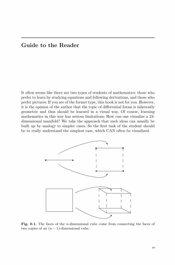
Fig. 0.1. The faces of the n-dimensional cube come from connecting the faces oftwo copies of an (n− 1)-dimensional cube.
xv
xvi Guide to the Reader
For example, suppose one wants to understand the combinatorics of then-dimensional cube. We can visualize a 1-D cube (i.e., an interval) and seejust from our mental picture that it has two boundary points. Next, we canvisualize a 2-D cube (a square) and see from our picture that this has fourintervals on its boundary. Furthermore, we see that we can construct this 2-Dcube by taking two parallel copies of our original 1-D cube and connectingthe endpoints. Since there are two endpoints, we get two new intervals, inaddition to the two we started with (see Figure 0.1). Now, to construct a 3-Dcube, we place two squares parallel to each other and connect up their edges.Each time we connect an edge of one square to an edge of the other, we geta new square on the boundary of the 3-D cube. Hence, since there were fouredges on the boundary of each square, we get four new squares, in addition tothe two we started with, making six in all. Now, if the student understandsthis, then it should not be hard to convince him/her that every time we goup a dimension, the number of lower-dimensional cubes on the boundary isthe same as in the previous dimension, plus two. Finally, from this we canconclude that there are 2n (n− 1)-dimensional cubes on the boundary of then-dimensional cube.
Note the strategy in the above example: We understand the “small” casesvisually and use them to generalize to the cases we cannot visualize. This willbe our approach in studying differential forms.
Perhaps this goes against some trends in mathematics in the last severalhundred years. After all, there were times when people took geometric intu-ition as proof and later found that their intuition was wrong. This gave riseto the formalists, who accepted nothing as proof that was not a sequenceof formally manipulated logical statements. We do not scoff at this point ofview. We make no claim that the above derivation for the number of (n− 1)-dimensional cubes on the boundary of an n-dimensional cube is actually aproof. It is only a convincing argument, that gives enough insight to actuallyproduce a proof. Formally, a proof would still need to be given. Unfortunately,all too often the classical math book begins the subject with the proof, whichhides all of the geometric intuition to which the above argument leads.
1
Introduction
1.1 So what is a differential form?
A differential form is simply this: an integrand. In other words, it is a thingwhich can be integrated over some (often complicated) domain. For exam-
ple, consider the following integral:1∫0
x2dx. This notation indicates that we
are integrating x2 over the interval [0, 1]. In this case, x2dx is a differentialform. If you have had no exposure to this subject, this may make you a littleuncomfortable. After all, in calculus we are taught that x2 is the integrand.The symbol “dx” is only there to delineate when the integrand has ended andwhat variable we are integrating with respect to. However, as an object initself, we are not taught any meaning for “dx.” Is it a function? Is it an op-erator on functions? Some professors call it an “infinitesimal” quantity. This
is very tempting. After all,1∫0
x2dx is defined to be the limit, as n → ∞, of
n∑i=1
x2i∆x, where xi are n evenly spaced points in the interval [0, 1] and
∆x = 1/n. When we take the limit, the symbol “∑
” becomes “∫,” and the
symbol “∆x” becomes “dx.” This implies that dx = lim∆x→0∆x, which isabsurd. lim∆x→0∆x = 0!! We are not trying to make the argument that thesymbol “dx” should be eliminated. It does have meaning. This is one of themany mysteries that this book will reveal.
One word of caution here: Not all integrands are differential forms. In fact,in Section 4.8 we will see how to calculate arc length and surface area. Thesecalculations involve integrands which are not differential forms. Differentialforms are simply natural objects to integrate and also the first that one shouldstudy. As we will see, this is much like beginning the study of all functions byunderstanding linear functions. The naive student may at first object to this,since linear functions are a very restrictive class. On the other hand, eventuallywe learn that any differentiable function (a much more general class) can be
DOI 10.1007/978-0-8176-830 - _1, © Springer Science+Business Media, LLC 20121,, D. Bachman A Geometric Approach to Differential Forms
4 7
2 1 Introduction
locally approximated by a linear function. Hence, in some sense, the linearfunctions are the most important ones. In the same way, one can make theargument that differential forms are the most important integrands.
1.2 Generalizing the integral
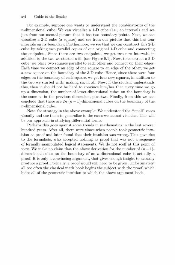
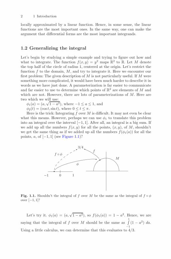
Let’s begin by studying a simple example and trying to figure out how andwhat to integrate. The function f(x, y) = y2 maps R
2 to R. Let M denotethe top half of the circle of radius 1, centered at the origin. Let’s restrict thefunction f to the domain, M , and try to integrate it. Here we encounter ourfirst problem: The given description ofM is not particularly useful. IfM weresomething more complicated, it would have been much harder to describe it inwords as we have just done. A parameterization is far easier to communicateand far easier to use to determine which points of R2 are elements of M andwhich are not. However, there are lots of parameterizations of M . Here aretwo which we will use:
φ1(a) = (a,√1− a2), where −1 ≤ a ≤ 1, and
φ2(t) = (cos t, sin t), where 0 ≤ t ≤ π.Here is the trick: Integrating f overM is difficult. It may not even be clear
what this means. However, perhaps we can use φ1 to translate this probleminto an integral over the interval [−1, 1]. After all, an integral is a big sum. Ifwe add up all the numbers f(x, y) for all the points, (x, y), of M , shouldn’twe get the same thing as if we added up all the numbers f(φ1(a)) for all thepoints, a, of [−1, 1] (see Figure 1.1)?
f
φ
f φ3/4
M
−1 10
Fig. 1.1. Shouldn’t the integral of f over M be the same as the integral of f φover [−1, 1]?
Let’s try it. φ1(a) = (a,√1− a2), so f(φ1(a)) = 1 − a2. Hence, we are
saying that the integral of f over M should be the same as1∫
−1
(1 − a2) da.
Using a little calculus, we can determine that this evaluates to 4/3.
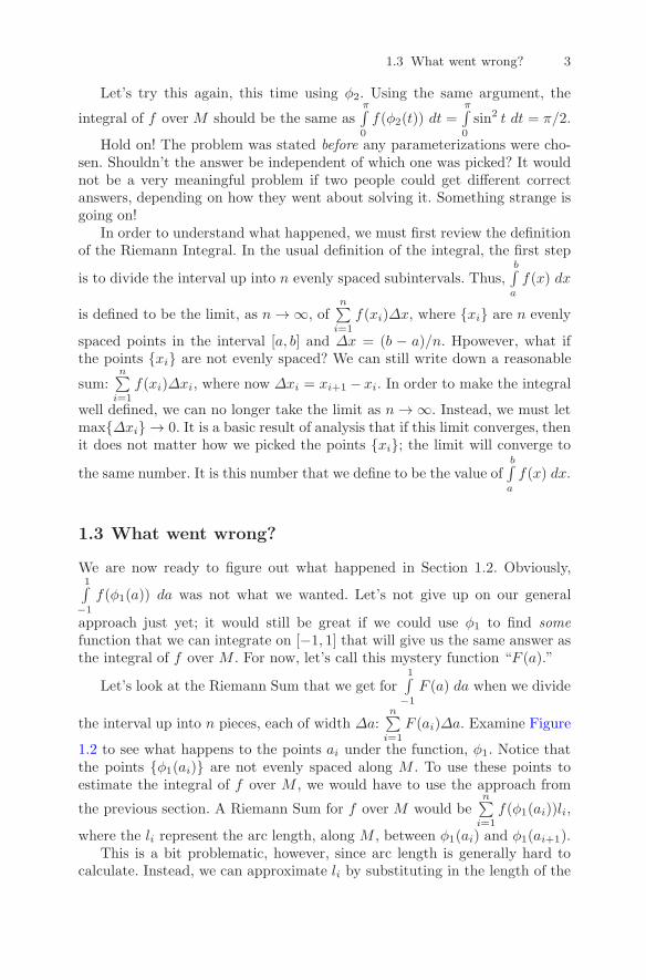
1.3 What went wrong? 3
Let’s try this again, this time using φ2. Using the same argument, the
integral of f over M should be the same asπ∫0
f(φ2(t)) dt =π∫0
sin2 t dt = π/2.
Hold on! The problem was stated before any parameterizations were cho-sen. Shouldn’t the answer be independent of which one was picked? It wouldnot be a very meaningful problem if two people could get different correctanswers, depending on how they went about solving it. Something strange isgoing on!
In order to understand what happened, we must first review the definitionof the Riemann Integral. In the usual definition of the integral, the first step
is to divide the interval up into n evenly spaced subintervals. Thus,b∫a
f(x) dx
is defined to be the limit, as n→ ∞, ofn∑i=1
f(xi)∆x, where xi are n evenly
spaced points in the interval [a, b] and ∆x = (b − a)/n. Hpowever, what ifthe points xi are not evenly spaced? We can still write down a reasonable
sum:n∑i=1
f(xi)∆xi, where now ∆xi = xi+1 − xi. In order to make the integral
well defined, we can no longer take the limit as n→ ∞. Instead, we must letmax∆xi → 0. It is a basic result of analysis that if this limit converges, thenit does not matter how we picked the points xi; the limit will converge to
the same number. It is this number that we define to be the value ofb∫a
f(x) dx.
1.3 What went wrong?
We are now ready to figure out what happened in Section 1.2. Obviously,1∫
−1
f(φ1(a)) da was not what we wanted. Let’s not give up on our general
approach just yet; it would still be great if we could use φ1 to find somefunction that we can integrate on [−1, 1] that will give us the same answer asthe integral of f over M . For now, let’s call this mystery function “F (a).”
Let’s look at the Riemann Sum that we get for1∫
−1
F (a) da when we divide
the interval up into n pieces, each of width ∆a:n∑i=1
F (ai)∆a. Examine Figure
1.2 to see what happens to the points ai under the function, φ1. Notice thatthe points φ1(ai) are not evenly spaced along M . To use these points toestimate the integral of f over M , we would have to use the approach from
the previous section. A Riemann Sum for f over M would ben∑i=1
f(φ1(ai))li,
where the li represent the arc length, along M , between φ1(ai) and φ1(ai+1).This is a bit problematic, however, since arc length is generally hard to
calculate. Instead, we can approximate li by substituting in the length of the
4 1 Introduction
f
φ
F (a2)
F
M
−1 1a2
f(φ(a2))
∆a
l1
l2 l3
l4L1
L2 L3
L4
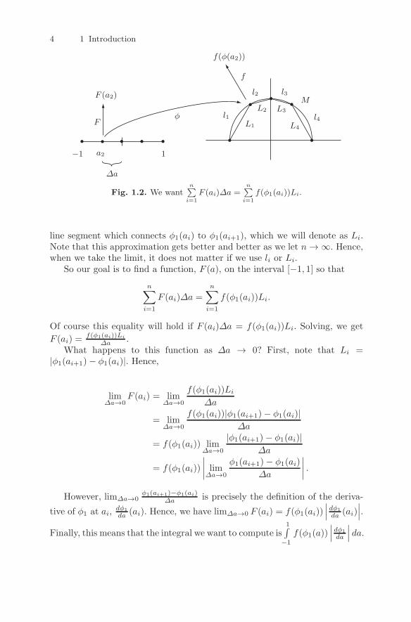
Fig. 1.2. We wantn∑
i=1
F (ai)∆a =n∑
i=1
f(φ1(ai))Li.
line segment which connects φ1(ai) to φ1(ai+1), which we will denote as Li.Note that this approximation gets better and better as we let n→ ∞. Hence,when we take the limit, it does not matter if we use li or Li.
So our goal is to find a function, F (a), on the interval [−1, 1] so that
n∑i=1
F (ai)∆a =
n∑i=1
f(φ1(ai))Li.
Of course this equality will hold if F (ai)∆a = f(φ1(ai))Li. Solving, we get
F (ai) =f(φ1(ai))Li
∆a .What happens to this function as ∆a → 0? First, note that Li =
|φ1(ai+1)− φ1(ai)|. Hence,
lim∆a→0
F (ai) = lim∆a→0
f(φ1(ai))Li∆a
= lim∆a→0
f(φ1(ai))|φ1(ai+1)− φ1(ai)|∆a
= f(φ1(ai)) lim∆a→0
|φ1(ai+1)− φ1(ai)|∆a
= f(φ1(ai))
∣∣∣∣ lim∆a→0
φ1(ai+1)− φ1(ai)
∆a
∣∣∣∣ .However, lim∆a→0
φ1(ai+1)−φ1(ai)∆a is precisely the definition of the deriva-
tive of φ1 at ai,dφ1
da (ai). Hence, we have lim∆a→0 F (ai) = f(φ1(ai))∣∣∣ dφ1
da (ai)∣∣∣.
Finally, this means that the integral we want to compute is1∫
−1
f(φ1(a))∣∣∣ dφ1
da
∣∣∣ da.
1.4 What about surfaces? 5
1.1. Check that1∫
−1
f(φ1(a))|dφ1
da | da =π∫0
f(φ2(t))|dφ2
dt | dt, using the function,
f , defined in Section 1.2.
Recall that dφ1
da is a vector, based at the point φ(a), tangent to M . If we
think of a as a time parameter, then the length of dφ1
da tells us how fast φ1(a)
is moving along M . How can we generalize the integral,1∫
−1
f(φ1(a))|dφ1
da | da?Note that the bars |·| denote a function that “eats” vectors and “spits out” realnumbers. So we can generalize the integral by looking at other such functions.
In other words, a more general integral would be1∫
−1
f(φ1(a))ω(dφ1
da ) da, where
f is a function of points and ω is a function of vectors.It is not the purpose of the present work to undertake a study of integrat-
ing with respect to all possible functions, ω. However, as with the study offunctions of real variables, a natural place to start is with linear functions.This is the study of differential forms. A differential form is precisely a linearfunction which eats vectors, spits out numbers and is used in integration. Thestrength of differential forms lies in the fact that their integrals do not dependon a choice of parameterization.
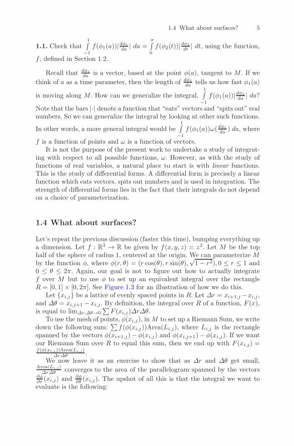
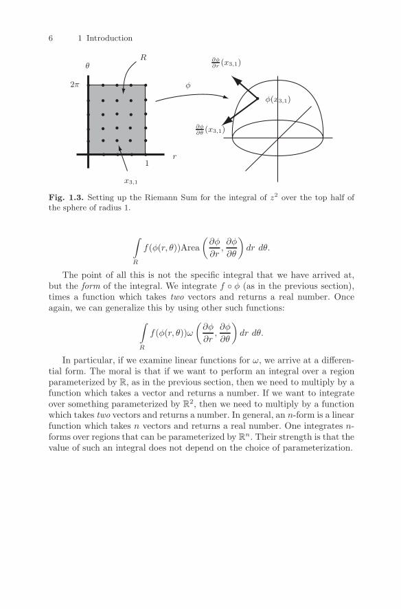
1.4 What about surfaces?
Let’s repeat the previous discussion (faster this time), bumping everything upa dimension. Let f : R3 → R be given by f(x, y, z) = z2. Let M be the tophalf of the sphere of radius 1, centered at the origin. We can parameterize Mby the function φ, where φ(r, θ) = (r cos(θ), r sin(θ),
√1− r2), 0 ≤ r ≤ 1 and
0 ≤ θ ≤ 2π. Again, our goal is not to figure out how to actually integratef over M but to use φ to set up an equivalent integral over the rectangleR = [0, 1]× [0, 2π]. See Figure 1.3 for an illustration of how we do this.
Let xi,j be a lattice of evenly spaced points in R. Let ∆r = xi+1,j−xi,j ,and ∆θ = xi,j+1 − xi,j . By definition, the integral over R of a function, F (x),is equal to lim∆r,∆θ→0
∑F (xi,j)∆r∆θ.
To use the mesh of points, φ(xi,j), inM to set up a Riemann Sum, we writedown the following sum:
∑f(φ(xi,j))Area(Li,j), where Li,j is the rectangle
spanned by the vectors φ(xi+1,j)− φ(xi,j) and φ(xi,j+1)− φ(xi,j). If we wantour Riemann Sum over R to equal this sum, then we end up with F (xi,j) =f(φ(xi,j))Area(Li,j)
∆r∆θ .We now leave it as an exercise to show that as ∆r and ∆θ get small,
Area(Li,j)∆r∆θ converges to the area of the parallelogram spanned by the vectors
∂φ∂r (xi,j) and ∂φ
∂θ (xi,j). The upshot of all this is that the integral we want toevaluate is the following:
6 1 Introduction
R
φ
r
θ
1
2π
x3,1
φ(x3,1)
∂φ∂r
(x3,1)
∂φ∂θ
(x3,1)
Fig. 1.3. Setting up the Riemann Sum for the integral of z2 over the top half ofthe sphere of radius 1.
∫R
f(φ(r, θ))Area
(∂φ
∂r,∂φ
∂θ
)dr dθ.
The point of all this is not the specific integral that we have arrived at,but the form of the integral. We integrate f φ (as in the previous section),times a function which takes two vectors and returns a real number. Onceagain, we can generalize this by using other such functions:∫
R
f(φ(r, θ))ω
(∂φ
∂r,∂φ
∂θ
)dr dθ.
In particular, if we examine linear functions for ω, we arrive at a differen-tial form. The moral is that if we want to perform an integral over a regionparameterized by R, as in the previous section, then we need to multiply by afunction which takes a vector and returns a number. If we want to integrateover something parameterized by R
2, then we need to multiply by a functionwhich takes two vectors and returns a number. In general, an n-form is a linearfunction which takes n vectors and returns a real number. One integrates n-forms over regions that can be parameterized by R
n. Their strength is that thevalue of such an integral does not depend on the choice of parameterization.
2
Prerequisites
2.1 Multivariable calculus
We denote by Rn the set of points with n real coordinates. In this text we will
often represent functions abstractly by saying how many numbers go into thefunction and how many come out. So, if we write f : Rn → R
m, we mean f isa function whose input is a point with n coordinates and whose output is apoint with m coordinates.
2.1. Sketch the graphs of the following functions f : R2 → R1:
1. z = 2x− 3y.2. z = x2 + y2.3. z = xy.4. z =
√x2 + y2.
5. z = 1√x2+y2
.
6. z =√x2 + y2 + 1.
7. z =√x2 + y2 − 1.
8. z = cos(x+ y).9. z = cos(xy).
10. z = cos(x2 + y2).
11. z = e−(x2+y2).
2.2. Find functions whose graphs are the following:
1. A plane through the origin at 45 to both the x- and y-axes.2. The top half of a sphere of radius 2.3. The top half of a torus centered around the z-axis (i.e., the tube of radius
1, say, centered around a circle of radius 2 in the xy-plane).4. The top half of the cylinder of radius 1 which is centered around the line
where the plane y = x meets the plane z = 0.
DOI 10.1007/978-0-8176-830 - _2, © Springer Science+Business Media, LLC 2012, D. Bachman
4 77,A Geometric Approach to Differential Forms
8 2 Prerequisites
You may find it helpful to check your answers to the above exercises witha computer graphing program.
The volume under the graph of a multivariable function is given by amultiple integral, as in the next example.
Example 1. To find the volume under the graph of f(x, y) = xy2 and abovethe rectangle R with vertices at (0, 0), (2, 0), (0, 3) and (2, 3) we compute
∫R
xy2 dx dy =
3∫0
2∫0
xy2 dx dy
=
3∫0
[1
2x2y2
∣∣∣∣2
x=0
]dy
=
3∫0
2y2 dy
= 18.
2.3. Let R be the rectangle in the xy-plane with vertices at (1, 0), (2, 0), (1, 3)and (2, 3). Integrate the following functions over R:
1. x2y2.2. 1.3. x2 + y2.
4.√x+ 2
3y.
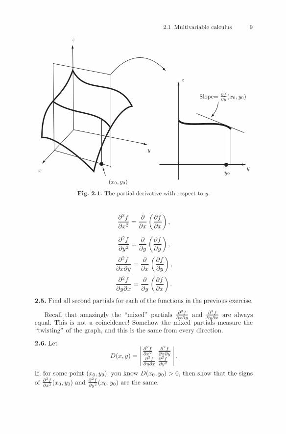
As in the one-variable case, derivates of multivariable functions give theslope of a tangent line. The relevant question here is “Which tangent line?”The answer to this is another question: “Which derivative?” For example,suppose we slice the graph of f : R2 → R
1 with the plane parallel to theyz-plane, through the point (x0, y0, 0). Then we get a curve which representssome function of y. We can then ask “What is the slope of the tangent lineto this curve when y = y0?” The answer to this question is precisely thedefinition of ∂f
∂y (x0, y0) (see Figure 2.1). Similarly, slicing the graph with a
plane parallel to the xz-plane gives rise to the definition of ∂f∂x (x0, y0).
2.4. Compute ∂f∂x and ∂f
∂y .
1. x2y3.2. sin(x2y3).3. x sin(xy).
When you take a partial derivative, you get another function of x and y.You can then do it again to find the second partials. These are denoted by
2.1 Multivariable calculus 9
y0x y
y
z
z
Slope= ∂f∂y
(x0, y0)
(x0, y0)
Fig. 2.1. The partial derivative with respect to y.
∂2f
∂x2=
∂
∂x
(∂f
∂x
),
∂2f
∂y2=
∂
∂y
(∂f
∂y
),
∂2f
∂x∂y=
∂
∂x
(∂f
∂y
),
∂2f
∂y∂x=
∂
∂y
(∂f
∂x
).
2.5. Find all second partials for each of the functions in the previous exercise.
Recall that amazingly the “mixed” partials ∂2f∂x∂y and ∂2f
∂y∂x are alwaysequal. This is not a coincidence! Somehow the mixed partials measure the“twisting” of the graph, and this is the same from every direction.
2.6. Let
D(x, y) =
∣∣∣∣∣∂2f∂x2
∂2f∂x∂y
∂2f∂y∂x
∂2f∂y2
∣∣∣∣∣ .If, for some point (x0, y0), you know D(x0, y0) > 0, then show that the signs
of ∂2f∂x2 (x0, y0) and
∂2f∂y2 (x0, y0) are the same.
10 2 Prerequisites
2.2 Gradients
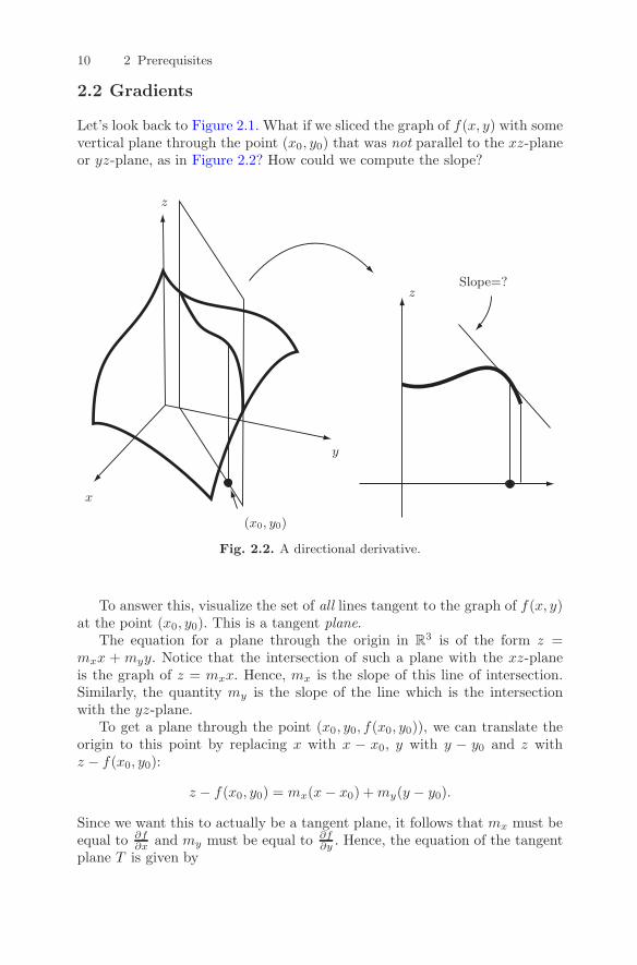
Let’s look back to Figure 2.1. What if we sliced the graph of f(x, y) with somevertical plane through the point (x0, y0) that was not parallel to the xz-planeor yz-plane, as in Figure 2.2? How could we compute the slope?
x
y
z
z
Slope=?
(x0, y0)
Fig. 2.2. A directional derivative.
To answer this, visualize the set of all lines tangent to the graph of f(x, y)at the point (x0, y0). This is a tangent plane.
The equation for a plane through the origin in R3 is of the form z =
mxx + myy. Notice that the intersection of such a plane with the xz-planeis the graph of z = mxx. Hence, mx is the slope of this line of intersection.Similarly, the quantity my is the slope of the line which is the intersectionwith the yz-plane.
To get a plane through the point (x0, y0, f(x0, y0)), we can translate theorigin to this point by replacing x with x − x0, y with y − y0 and z withz − f(x0, y0):
z − f(x0, y0) = mx(x− x0) +my(y − y0).
Since we want this to actually be a tangent plane, it follows that mx must beequal to ∂f
∂x and my must be equal to ∂f∂y . Hence, the equation of the tangent
plane T is given by
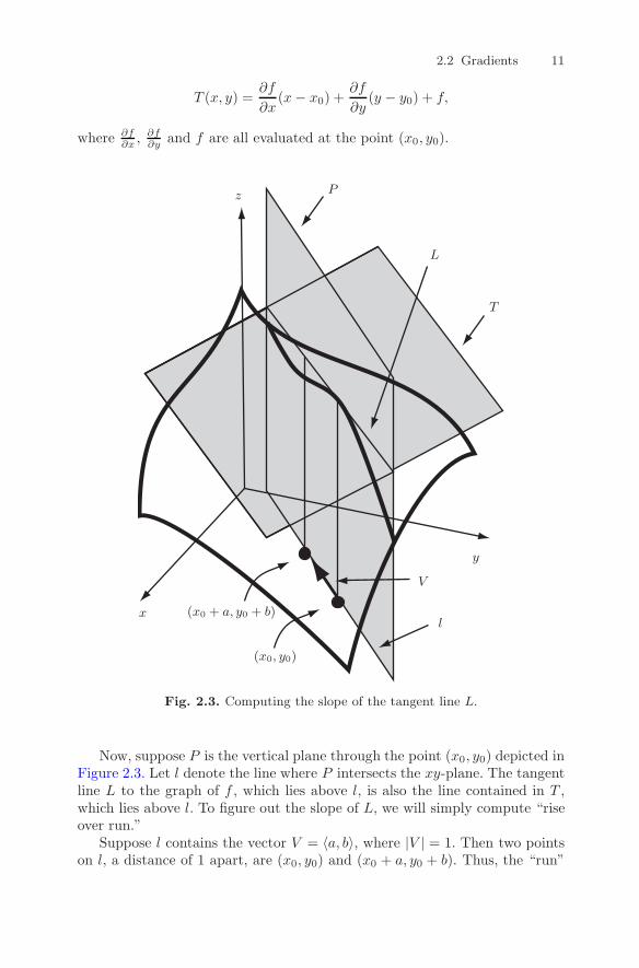
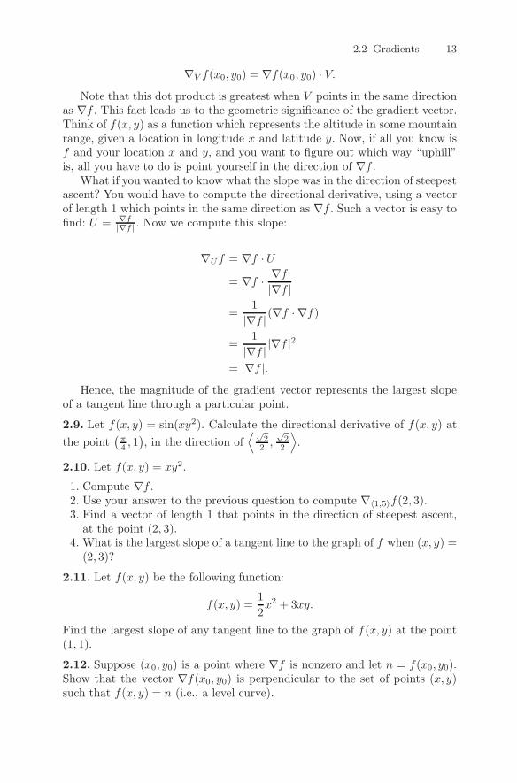
2.2 Gradients 11
T (x, y) =∂f
∂x(x− x0) +
∂f
∂y(y − y0) + f,
where ∂f∂x ,
∂f∂y and f are all evaluated at the point (x0, y0).
x
y
z
(x0, y0)
L
l
P
T
V
(x0 + a, y0 + b)
Fig. 2.3. Computing the slope of the tangent line L.
Now, suppose P is the vertical plane through the point (x0, y0) depicted inFigure 2.3. Let l denote the line where P intersects the xy-plane. The tangentline L to the graph of f , which lies above l, is also the line contained in T ,which lies above l. To figure out the slope of L, we will simply compute “riseover run.”
Suppose l contains the vector V = 〈a, b〉, where |V | = 1. Then two pointson l, a distance of 1 apart, are (x0, y0) and (x0 + a, y0 + b). Thus, the “run”
12 2 Prerequisites
will be equal to 1. The “rise” is the difference between T (x0, y0) and T (x0 +a, y0 + b), which we compute as follows:
T (x0 + a, y0 + b)− T (x0, y0)
=
[∂f
∂x(x0 + a− x0) +
∂f
∂y(y0 + b− y0) + f
]
−[∂f
∂x(x0 − x0) +
∂f
∂y(y0 − y0) + f
]
= a∂f
∂x+ b
∂f
∂y.
Since the slope of L is “rise” over “run” and the “run” equals 1, we concludethat the slope of L is a∂f
∂x + b∂f∂y , where∂f∂x and ∂f
∂y are evaluated at the point
(x0, y0).
2.7. Suppose f(x, y) = x2y3. Compute the slope of the line tangent to f(x, y),
at the point (2, 1), in the direction 〈√22 ,−
√22 〉.
The quantity a∂f∂x (x0, y0) + b∂f∂y (x0, y0) is defined to be the directional
derivative of f , at the point (x0, y0), in the direction V . We will adopt thenotation ∇V f(x0, y0) for this quantity.
Let f(x, y) = xy2. Let’s compute the directional derivative of f , at thepoint (2, 3), in the direction V = 〈1, 5〉. We compute
∇V f(2, 3) = 1∂f
∂x(2, 3) + 5
∂f
∂y(2, 3)
= 1 · 32 + 5 · 2 · 2 · 3= 69.
Is 69 the slope of the tangent line to some curve that we get when we intersectthe graph of xy2 with some plane? What this number represents is the rate ofchange of f , as we walk along the line l of Figure 2.3 with speed |V |. To findthe desired slope, we would have to walk with speed 1. Hence, the directionalderivative only represents a slope when |V | = 1.
2.8. Let f(x, y) = xy + x − 2y + 4. Find the slope of the tangent line to thegraph of f(x, y), in the direction of the vector 〈1, 2〉, at the point (0, 1).
To proceed further, we write the definition of ∇V f as a dot product:
∇〈a,b〉f(x0, y0) = a∂f
∂x+ b
∂f
∂y=
⟨∂f
∂x,∂f
∂y
⟩· 〈a, b〉.
The vector⟨∂f∂x ,
∂f∂y
⟩is called the gradient of f and is denoted ∇f . Using
this notation, we obtain the following formula:
2.2 Gradients 13
∇V f(x0, y0) = ∇f(x0, y0) · V.Note that this dot product is greatest when V points in the same direction
as ∇f . This fact leads us to the geometric significance of the gradient vector.Think of f(x, y) as a function which represents the altitude in some mountainrange, given a location in longitude x and latitude y. Now, if all you know isf and your location x and y, and you want to figure out which way “uphill”is, all you have to do is point yourself in the direction of ∇f .
What if you wanted to know what the slope was in the direction of steepestascent? You would have to compute the directional derivative, using a vectorof length 1 which points in the same direction as ∇f . Such a vector is easy tofind: U = ∇f
|∇f | . Now we compute this slope:
∇Uf = ∇f · U= ∇f · ∇f
|∇f |=
1
|∇f | (∇f · ∇f)
=1
|∇f | |∇f |2
= |∇f |.Hence, the magnitude of the gradient vector represents the largest slope
of a tangent line through a particular point.
2.9. Let f(x, y) = sin(xy2). Calculate the directional derivative of f(x, y) at
the point(π4 , 1
), in the direction of
⟨√22 ,
√22
⟩.
2.10. Let f(x, y) = xy2.
1. Compute ∇f .2. Use your answer to the previous question to compute ∇〈1,5〉f(2, 3).3. Find a vector of length 1 that points in the direction of steepest ascent,
at the point (2, 3).4. What is the largest slope of a tangent line to the graph of f when (x, y) =
(2, 3)?
2.11. Let f(x, y) be the following function:
f(x, y) =1
2x2 + 3xy.
Find the largest slope of any tangent line to the graph of f(x, y) at the point(1, 1).
2.12. Suppose (x0, y0) is a point where ∇f is nonzero and let n = f(x0, y0).Show that the vector ∇f(x0, y0) is perpendicular to the set of points (x, y)such that f(x, y) = n (i.e., a level curve).
14 2 Prerequisites
2.3 Polar, cylindrical and spherical coordinates
The two most common ways of specifying the location of a point in R2 are
rectangular and polar coordinates. Rectangular coordinates on R2 will always
be denoted in this text as (x, y) and polar coordinates by (r, θ). As is standard,r is the distance to the origin and θ is the angle a ray makes with the (pos-itive) x-axis. Some basic trigonometry gives the relationships between thesequantities:
x = r cos θ r =√x2 + y2,
y = r sin θ θ = tan−1(yx
).
In R3 we will mostly use three different coordinate systems: rectangular
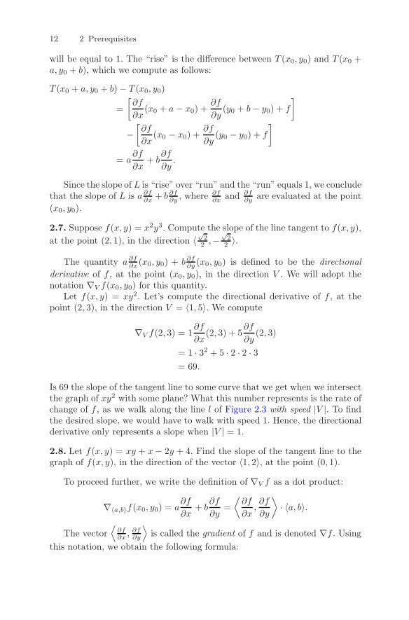
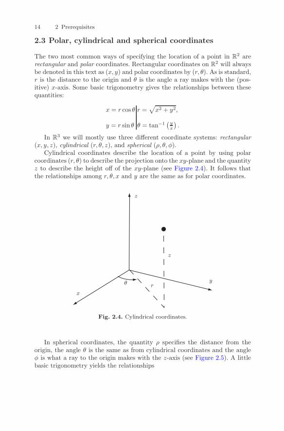
(x, y, z), cylindrical (r, θ, z), and spherical (ρ, θ, φ).Cylindrical coordinates describe the location of a point by using polar
coordinates (r, θ) to describe the projection onto the xy-plane and the quantityz to describe the height off of the xy-plane (see Figure 2.4). It follows thatthe relationships among r, θ, x and y are the same as for polar coordinates.
x
y
z
z
rθ
Fig. 2.4. Cylindrical coordinates.
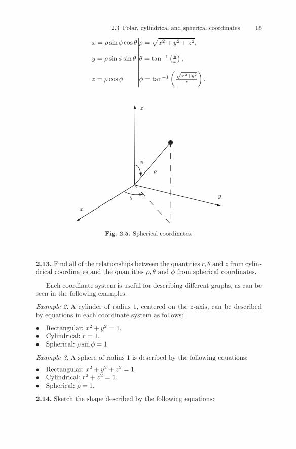
In spherical coordinates, the quantity ρ specifies the distance from theorigin, the angle θ is the same as from cylindrical coordinates and the angleφ is what a ray to the origin makes with the z-axis (see Figure 2.5). A littlebasic trigonometry yields the relationships
2.3 Polar, cylindrical and spherical coordinates 15
x = ρ sinφ cos θ ρ =√x2 + y2 + z2,
y = ρ sinφ sin θ θ = tan−1(yx
),
z = ρ cosφ φ = tan−1
(√x2+y2
z
).
x
y
z
ρ
θ
φ
Fig. 2.5. Spherical coordinates.
2.13. Find all of the relationships between the quantities r, θ and z from cylin-drical coordinates and the quantities ρ, θ and φ from spherical coordinates.
Each coordinate system is useful for describing different graphs, as can beseen in the following examples.
Example 2. A cylinder of radius 1, centered on the z-axis, can be describedby equations in each coordinate system as follows:
• Rectangular: x2 + y2 = 1.• Cylindrical: r = 1.• Spherical: ρ sinφ = 1.
Example 3. A sphere of radius 1 is described by the following equations:
• Rectangular: x2 + y2 + z2 = 1.• Cylindrical: r2 + z2 = 1.• Spherical: ρ = 1.
2.14. Sketch the shape described by the following equations:
16 2 Prerequisites
1. θ = π4 .
2. z = r2.3. ρ = φ.4. ρ = cosφ.5. r = cos θ.6. z =
√r2 − 1.
7. z =√r2 + 1.
8. r = θ.
2.15. Find rectangular, cylindrical and spherical equations that describe thefollowing shapes:
1. A right, circular cone centered on the z-axis, with vertex at the origin.2. The xz-plane.3. The xy-plane.4. A plane that is at an angle of π
4 with both the x- and y-axes.5. The surface found by revolving the graph of z = x3 (where x ≥ 0) around
the z-axis.
2.16. Let S be the surface which is the graph of z =√r2 + 1 (in cylindrical
coordinates).
1. Describe and/or sketch S.2. Write an equation for S in rectangular coordinates.
2.4 Parameterized curves
Given a curve C in Rn, a parameterization for C is a (one-to-one, onto, dif-
ferentiable) function of the form φ : R1 → Rn whose image is C.
Example 4. The function φ(t) = (cos t, sin t), where 0 ≤ t < 2π, is a param-eterization for the circle of radius 1. Another parameterization for the samecircle is ψ(t) = (cos 2t, sin 2t), where 0 ≤ t < π. The difference between thesetwo parameterizations is that as t increases, the image of ψ(t) moves twice asfast around the circle as the image of φ(t).
2.17. A function of the form φ(t) = (at+ c, bt+ d) is a parameterization of aline.
1. What is the slope of the line parameterized by φ?2. How does this line compare to the one parameterized by ψ(t) = (at, bt)?
2.18. Draw the curves given by the following parameterizations:
1. (t, t2), where 0 ≤ t ≤ 1.2. (t2, t3), where 0 ≤ t ≤ 1.3. (2 cos t, 3 sin t), where 0 ≤ t ≤ 2π.
2.4 Parameterized curves 17
4. (cos 2t, sin 3t), where 0 ≤ t ≤ 2π.5. (t cos t, t sin t), where 0 ≤ t ≤ 2π.
Given a curve, it can be very difficult to find a parameterization. Thereare many ways of approaching the problem, but nothing which always works.Here are a few hints:
1. If C is the graph of a function y = f(x), then φ(t) = (t, f(t)) is a param-eterization of C. Notice that the y-coordinate of every point in the imageof this parameterization is obtained from the x-coordinate by applyingthe function f .
2. If one has a polar equation for a curve like r = f(θ), then, since x =r cos θ and y = r sin θ, we get a parameterization of the form φ(θ) =(f(θ) cos θ, f(θ) sin θ).
Example 5. The top half of a circle of radius 1 is the graph of y =√1− x2.
Hence, a parameterization for this is (t,√1− t2), where −1 ≤ t ≤ 1. This
figure is also the graph of the polar equation r = 1, 0 ≤ θ ≤ π, hence theparameterization (cos t, sin t), where 0 ≤ t ≤ π.
2.19. Sketch and find parameterizations for the curves described by the fol-lowing:
1. The graph of the polar equation r = cos θ.2. The graph of y = sinx.3. The set of points such that x = sin y.
2.20. Find a parameterization for the line segment which connects the point(1, 1) to the point (2, 5).
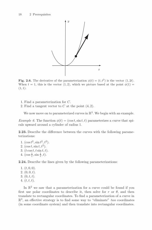
The derivative of a parameterization φ(t) = (f(t), g(t)) is defined to bethe vector
φ′(t) =dφ
dt=
d
dt(f(t), g(t)) = 〈f ′(t), g′(t)〉.
This vector has important geometric significance. The slope of a line con-taining this vector when t = t0 is the same as the slope of the line tangentto the curve at the point φ(t0). The magnitude (length) of this vector givesone a concept of the speed of the point φ(t) as t is increases through t0. Forconvenience, one often draws the vector φ′(t0) based at the point φ(t0) (seeFigure 2.6).
2.21. Let φ(t) = (cos t, sin t) (where 0 ≤ t ≤ π) and ψ(t) = (t,√1− t2) (where
−1 ≤ t ≤ 1) be parameterizations of the top half of the unit circle. Sketch the
vectors dφdt and dψ
dt at the points (√22 ,
√22 ), (0, 1) and (−
√22 ,
√22 ).
2.22. Let C be the set of points in R2 that satisfy the equation x = y2.
18 2 Prerequisites
x
y
Fig. 2.6. The derivative of the parameterization φ(t) = (t, t2) is the vector 〈1, 2t〉.When t = 1, this is the vector 〈1, 2〉, which we picture based at the point φ(1) =(1, 1).
1. Find a parameterization for C.2. Find a tangent vector to C at the point (4, 2).
We nowmove on to parameterized curves in R3. We begin with an example.
Example 6. The function φ(t) = (cos t, sin t, t) parameterizes a curve that spi-rals upward around a cylinder of radius 1.
2.23. Describe the difference between the curves with the following parame-terizations:
1. (cos t2, sin t2, t2).2. (cos t, sin t, t2).3. (t cos t, t sin t, t).4. (cos 1
t , sin1t , t).
2.24. Describe the lines given by the following parameterizations:
1. (t, 0, 0).2. (0, 0, t).3. (0, t, t).4. (t, t, t).
In R2 we saw that a parameterization for a curve could be found if you
first use polar coordinates to describe it, then solve for r or θ, and thentranslate to rectangular coordinates. To find a parameterization of a curve inR
3, an effective strategy is to find some way to “eliminate” two coordinates(in some coordinate system) and then translate into rectangular coordinates.
2.5 Parameterized surfaces in R3 19
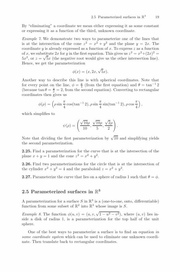
By “eliminating” a coordinate we mean either expressing it as some constantor expressing it as a function of the third, unknown coordinate.
Example 7. We demonstrate two ways to parameterize one of the lines thatis at the intersection of the cone z2 = x2 + y2 and the plane y = 2x. Thecoordinate y is already expressed as a function of x. To express z as a functionof x, we substitute 2x for y in the first equation. This gives us z2 = x2+(2x)2 =5x2, or z =
√5x (the negative root would give us the other intersection line).
Hence, we get the parameterization
φ(x) = (x, 2x,√5x).
Another way to describe this line is with spherical coordinates. Note thatfor every point on the line, φ = π
4 (from the first equation) and θ = tan−1 2(because tan θ = y
x = 2, from the second equation). Converting to rectangularcoordinates then gives us
φ(ρ) =(ρ sin
π
4cos(tan−1 2), ρ sin
π
4sin(tan−1 2), ρ cos
π
4
),
which simplifies to
ψ(ρ) =
(√10ρ
10,
√10ρ
5,
√2ρ
2
).
Note that dividing the first parameterization by√10 and simplifying yields
the second parameterization.
2.25. Find a parameterization for the curve that is at the intersection of theplane x+ y = 1 and the cone z2 = x2 + y2.
2.26. Find two parameterizations for the circle that is at the intersection ofthe cylinder x2 + y2 = 4 and the paraboloid z = x2 + y2.
2.27. Parameterize the curve that lies on a sphere of radius 1 such that θ = φ.
2.5 Parameterized surfaces in R3
A parameterization for a surface S in R3 is a (one-to-one, onto, differentiable)
function from some subset of R2 into R3 whose image is S.
Example 8. The function φ(u, v) = (u, v,√1− u2 − v2), where (u, v) lies in-
side a disk of radius 1, is a parameterization for the top half of the unitsphere.
One of the best ways to parameterize a surface is to find an equation insome coordinate system which can be used to eliminate one unknown coordi-nate. Then translate back to rectangular coordinates.
20 2 Prerequisites
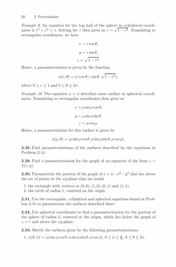
Example 9. An equation for the top half of the sphere in cylindrical coordi-nates is r2 + z2 = 1. Solving for z then gives us z =
√1− r2. Translating to
rectangular coordinates, we have
x = r cos θ,
y = r sin θ,
z =√
1− r2.
Hence, a parameterization is given by the function
φ(r, θ) = (r cos θ, r sin θ,√
1− r2),
where 0 ≤ r ≤ 1 and 0 ≤ θ ≤ 2π.
Example 10. The equation ρ = φ describes some surface in spherical coordi-nates. Translating to rectangular coordinates then gives us
x = ρ sin ρ cos θ,
y = ρ sin ρ sin θ,
z = ρ cos ρ.
Hence, a parameterization for this surface is given by
φ(ρ, θ) = (ρ sin ρ cos θ, ρ sin ρ sin θ, ρ cosρ).
2.28. Find parameterizations of the surfaces described by the equations inProblem 2.14.
2.29. Find a parameterization for the graph of an equation of the form z =f(x, y).
2.30. Parameterize the portion of the graph of z = 4−x2− y2 that lies abovethe set of points in the xy-plane that are inside
1. the rectangle with vertices at (0, 0), (1, 0), (0, 1) and (1, 1).2. the circle of radius 1, centered on the origin.
2.31. Use the rectangular, cylindrical and spherical equations found in Prob-lem 2.15 to parameterize the surfaces described there.
2.32. Use spherical coordinates to find a parameterization for the portion ofthe sphere of radius 2, centered at the origin, which lies below the graph ofz = r and above the xy-plane.
2.33. Sketch the surfaces given by the following parameterizations:
1. ψ(θ, φ) = (φ sin φ cos θ, φ sinφ sin θ, φ cosφ), 0 ≤ φ ≤ π2 , 0 ≤ θ ≤ 2π.
2.6 Parameterized regions in R2 and R
3 21
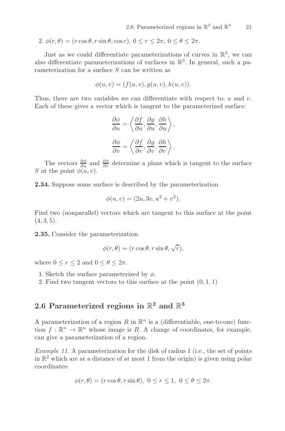
2. φ(r, θ) = (r cos θ, r sin θ, cos r), 0 ≤ r ≤ 2π, 0 ≤ θ ≤ 2π.
Just as we could differentiate parameterizations of curves in R2, we can
also differentiate parameterizations of surfaces in R3. In general, such a pa-
rameterization for a surface S can be written as
φ(u, v) = (f(u, v), g(u, v), h(u, v)).
Thus, there are two variables we can differentiate with respect to: u and v.Each of these gives a vector which is tangent to the parameterized surface:
∂φ
∂u=
⟨∂f
∂u,∂g
∂u,∂h
∂u
⟩,
∂φ
∂v=
⟨∂f
∂v,∂g
∂v,∂h
∂v
⟩.
The vectors ∂φ∂u and ∂φ
∂v determine a plane which is tangent to the surfaceS at the point φ(u, v).
2.34. Suppose some surface is described by the parameterization
φ(u, v) = (2u, 3v, u2 + v2).
Find two (nonparallel) vectors which are tangent to this surface at the point(4, 3, 5).
2.35. Consider the parameterization
φ(r, θ) = (r cos θ, r sin θ,√r),
where 0 ≤ r ≤ 2 and 0 ≤ θ ≤ 2π.
1. Sketch the surface parameterized by φ.2. Find two tangent vectors to this surface at the point (0, 1, 1)
2.6 Parameterized regions in R2 and R
3
A parameterization of a region R in Rn is a (differentiable, one-to-one) func-
tion f : Rn → Rn whose image is R. A change of coordinates, for example,
can give a parameterization of a region.
Example 11. A parameterization for the disk of radius 1 (i.e., the set of pointsin R
2 which are at a distance of at most 1 from the origin) is given using polarcoordinates:
φ(r, θ) = (r cos θ, r sin θ), 0 ≤ r ≤ 1, 0 ≤ θ ≤ 2π.
22 2 Prerequisites
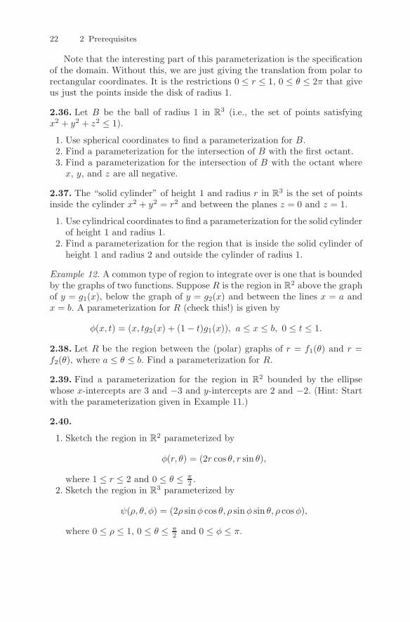
Note that the interesting part of this parameterization is the specificationof the domain. Without this, we are just giving the translation from polar torectangular coordinates. It is the restrictions 0 ≤ r ≤ 1, 0 ≤ θ ≤ 2π that giveus just the points inside the disk of radius 1.
2.36. Let B be the ball of radius 1 in R3 (i.e., the set of points satisfying
x2 + y2 + z2 ≤ 1).
1. Use spherical coordinates to find a parameterization for B.2. Find a parameterization for the intersection of B with the first octant.3. Find a parameterization for the intersection of B with the octant wherex, y, and z are all negative.
2.37. The “solid cylinder” of height 1 and radius r in R3 is the set of points
inside the cylinder x2 + y2 = r2 and between the planes z = 0 and z = 1.
1. Use cylindrical coordinates to find a parameterization for the solid cylinderof height 1 and radius 1.
2. Find a parameterization for the region that is inside the solid cylinder ofheight 1 and radius 2 and outside the cylinder of radius 1.
Example 12. A common type of region to integrate over is one that is boundedby the graphs of two functions. Suppose R is the region in R
2 above the graphof y = g1(x), below the graph of y = g2(x) and between the lines x = a andx = b. A parameterization for R (check this!) is given by
φ(x, t) = (x, tg2(x) + (1− t)g1(x)), a ≤ x ≤ b, 0 ≤ t ≤ 1.
2.38. Let R be the region between the (polar) graphs of r = f1(θ) and r =f2(θ), where a ≤ θ ≤ b. Find a parameterization for R.
2.39. Find a parameterization for the region in R2 bounded by the ellipse
whose x-intercepts are 3 and −3 and y-intercepts are 2 and −2. (Hint: Startwith the parameterization given in Example 11.)
2.40.
1. Sketch the region in R2 parameterized by
φ(r, θ) = (2r cos θ, r sin θ),
where 1 ≤ r ≤ 2 and 0 ≤ θ ≤ π2 .
2. Sketch the region in R3 parameterized by
ψ(ρ, θ, φ) = (2ρ sinφ cos θ, ρ sinφ sin θ, ρ cosφ),
where 0 ≤ ρ ≤ 1, 0 ≤ θ ≤ π2 and 0 ≤ φ ≤ π.
2.6 Parameterized regions in R2 and R
3 23
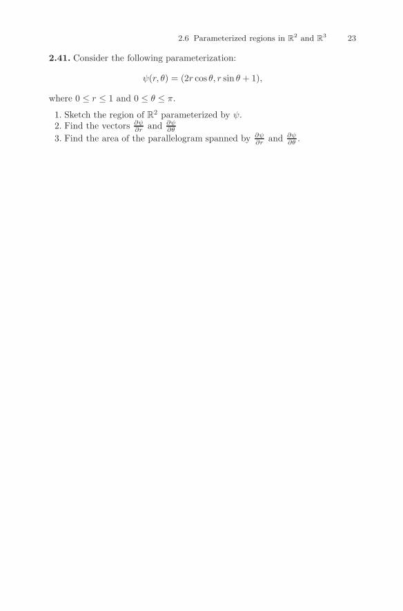
2.41. Consider the following parameterization:
ψ(r, θ) = (2r cos θ, r sin θ + 1),
where 0 ≤ r ≤ 1 and 0 ≤ θ ≤ π.
1. Sketch the region of R2 parameterized by ψ.2. Find the vectors ∂ψ
∂r and ∂ψ∂θ
3. Find the area of the parallelogram spanned by ∂ψ∂r and ∂ψ
∂θ .

3
Forms
3.1 Coordinates for vectors
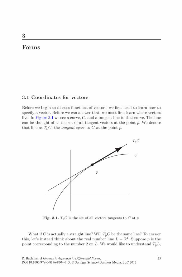
Before we begin to discuss functions of vectors, we first need to learn how tospecify a vector. Before we can answer that, we must first learn where vectorslive. In Figure 3.1 we see a curve, C, and a tangent line to that curve. The linecan be thought of as the set of all tangent vectors at the point p. We denotethat line as TpC, the tangent space to C at the point p.
TpC
p
C
Fig. 3.1. TpC is the set of all vectors tangents to C at p.
What if C is actually a straight line? Will TpC be the same line? To answerthis, let’s instead think about the real number line L = R
1. Suppose p is thepoint corresponding to the number 2 on L. We would like to understand TpL,
DOI 10.1007/978-0-8176-830 - _3, © Springer Science+Business Media, LLC 2012, D. Bachman
4 725,A Geometric Approach to Differential Forms
26 3 Forms
the set of all vectors tangent to L at the point p. For example, where wouldyou draw a vector of length 3? Would you put its base at the origin on L? Ofcourse not. You would put its base at the point p. This is really because theorigin for TpL is different than the origin for L. We are thus thinking aboutL and TpL as two different lines, placed right on top of each other.
The key to understanding the difference between L and TpL is their co-ordinate systems. Let’s pause here for a moment to look a little more closely.What are “coordinates” anyway? They are a way of assigning a number (or,more generally, a set of numbers) to a point in space. In other words, coordi-nates are functions which take points of a space and return (sets of) numbers.When we say that the x-coordinate of p in R
2 is 5, we really mean that wehave a function x : R2 → R, such that x(p) = 5.
Of course we need two numbers to specify a point in a plane, which meansthat we have two coordinate functions. Suppose we denote the plane by Pand x : P → R and y : P → R are our coordinate functions. Then, sayingthat the coordinates of a point, p, are (2, 3) is the same thing as saying thatx(p) = 2 and y(p) = 3. In other words, the coordinates of p are (x(p), y(p)).
So what do we use for coordinates in the tangent space? Well, first weneed a basis for the tangent space of P at p. In other words, we need topick two vectors which we can use to give the relative positions of all other
points. Note that if the coordinates of p are (x, y), then d(x+t,y)dt = 〈1, 0〉 and
d(x,y+t)dt = 〈0, 1〉. We have switched to the notation “〈·, ·〉” to indicate that
we are not talking about points of P anymore, but rather vectors in TpP . Wetake these two vectors to be a basis for TpP . In other words, any point of TpPcan be written as dx〈0, 1〉+ dy〈1, 0〉, where dx, dy ∈ R. Hence, “dx” and “dy”are coordinate functions for TpP . Saying that the coordinates of a vector V inTpP are 〈2, 3〉, for example, is the same thing as saying that dx(V ) = 2 anddy(V ) = 3. In general, we may refer to the coordinates of an arbitrary vectorin TpP as 〈dx, dy〉, just as we may refer to the coordinates of an arbitrarypoint in P as (x, y).
It will be helpful in the future to be able to distinguish between the vector〈2, 3〉 in TpP and the vector 〈2, 3〉 in TqP , where p = q. We will do this bywriting 〈2, 3〉p for the former and 〈2, 3〉q for the latter.
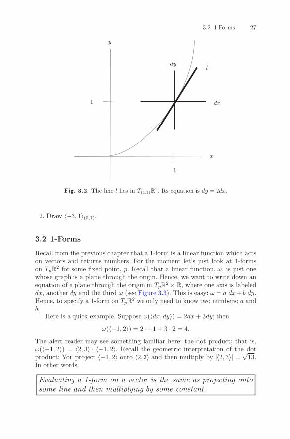
Let’s pause for a moment to address something that may have been both-ering you since your first term of calculus. Let’s look at the tangent line tothe graph of y = x2 at the point (1, 1). We are no longer thinking of thistangent line as lying in the same plane that the graph does. Rather, it liesin T(1,1)R
2. The horizontal axis for T(1,1)R2 is the “dx” axis and the vertical
axis is the “dy” axis (see Figure 3.2). Hence, we can write the equation of thetangent line as dy = 2dx. We can rewrite this as dy
dx = 2. Look familiar? This
is one explanation for why we use the notation dydx in calculus to denote the
derivative.
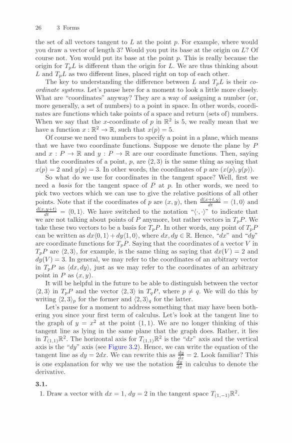
3.1.
1. Draw a vector with dx = 1, dy = 2 in the tangent space T(1,−1)R2.
3.2 1-Forms 27
x
y
l
dx
dy
1
1
Fig. 3.2. The line l lies in T(1,1)R2. Its equation is dy = 2dx.
2. Draw 〈−3, 1〉(0,1).
3.2 1-Forms
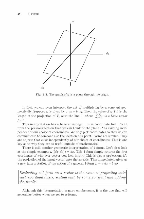
Recall from the previous chapter that a 1-form is a linear function which actson vectors and returns numbers. For the moment let’s just look at 1-formson TpR
2 for some fixed point, p. Recall that a linear function, ω, is just onewhose graph is a plane through the origin. Hence, we want to write down anequation of a plane through the origin in TpR
2 ×R, where one axis is labeleddx, another dy and the third ω (see Figure 3.3). This is easy: ω = a dx+ b dy.Hence, to specify a 1-form on TpR
2 we only need to know two numbers: a andb.
Here is a quick example. Suppose ω(〈dx, dy〉) = 2dx+ 3dy; then
ω(〈−1, 2〉) = 2 · −1 + 3 · 2 = 4.
The alert reader may see something familiar here: the dot product; that is,ω(〈−1, 2〉) = 〈2, 3〉 · 〈−1, 2〉. Recall the geometric interpretation of the dotproduct: You project 〈−1, 2〉 onto 〈2, 3〉 and then multiply by |〈2, 3〉| = √
13.In other words:
Evaluating a 1-form on a vector is the same as projecting ontosome line and then multiplying by some constant.
28 3 Forms
dx
dy
ω
Fig. 3.3. The graph of ω is a plane through the origin.
In fact, we can even interpret the act of multiplying by a constant geo-metrically. Suppose ω is given by a dx+ b dy. Then the value of ω(V1) is the
length of the projection of V1 onto the line, l, where 〈a,b〉|〈a,b〉|2 is a basis vector
for l.This interpretation has a huge advantage ... it is coordinate free. Recall
from the previous section that we can think of the plane P as existing inde-pendent of our choice of coordinates. We only pick coordinates so that we cancommunicate to someone else the location of a point. Forms are similar. Theyare objects that exist independently of our choice of coordinates. This is onekey as to why they are so useful outside of mathematics.
There is still another geometric interpretation of 1-forms. Let’s first lookat the simple example ω(〈dx, dy〉) = dx. This 1-form simply returns the firstcoordinate of whatever vector you feed into it. This is also a projection; it’sthe projection of the input vector onto the dx-axis. This immediately gives usa new interpretation of the action of a general 1-form ω = a dx+ b dy.
Evaluating a 1-form on a vector is the same as projecting ontoeach coordinate axis, scaling each by some constant and addingthe results.
Although this interpretation is more cumbersome, it is the one that willgeneralize better when we get to n-forms.
3.3 Multiplying 1-forms 29
Let’s move on now to 1-forms in n dimensions. If p ∈ Rn, then we can write
p in coordinates as (x1, x2, ..., xn). The coordinates for a vector in TpRn are
〈dx1, dx2, ..., dxn〉. A 1-form is a linear function, ω, whose graph (in TpRn×R)
is a plane through the origin. Hence, we can write it as ω = a1 dx1+a2 dx2+· · ·+an dxn. Again, this can be thought of as either projecting onto the vector〈a1, a2, ..., an〉 and then multiplying by |〈a1, a2, ..., an〉| or as projecting ontoeach coordinate axis, multiplying by ai, and then adding.
3.2. Let ω(〈dx, dy〉) = −dx+ 4dy.
1. Compute ω(〈1, 0〉), ω(〈0, 1〉) and ω(〈2, 3〉).2. What line does ω project vectors onto?
3.3. Find a 1-form which computes the length of the projection of a vectoronto the indicated line, multiplied by the indicated constant c.
1. The dx-axis, c = 3.2. The dy-axis, c = 1
2 .3. Find a 1-form that does both of the two preceding operations and adds
the result.4. The line dy = 3
4dx, c = 10.
3.4. If ω is a 1-form show the following:
1. ω(V1 + V2) = ω(V1) + ω(V2), for any vectors V1 and V2.2. ω(cV ) = cω(V ), for any vector V and constant c.
3.3 Multiplying 1-forms
In this section we would like to explore a method of multiplying 1-forms. Youmay think “What is the big deal? If ω and ν are 1-forms, can’t we just defineω · ν(V ) = ω(V ) · ν(V )?” Well, of course we can, but then ω · ν is not a linearfunction, so we have left the world of forms.
The trick is to define the product of ω and ν to be a 2-form. So as notto confuse this with the product just mentioned, we will use the symbol “∧”(pronounced “wedge”) to denote multiplication. So how can we possibly defineω∧ν to be a 2-form? We must define how it acts on a pair of vectors, (V1, V2).
Note first that there are four ways to combine all of the ingredients:
ω(V1), ν(V1), ω(V2), ν(V2).
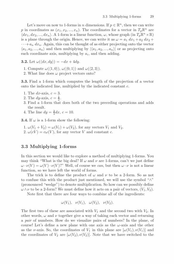
The first two of these are associated with V1 and the second two with V2. Inother words, ω and ν together give a way of taking each vector and returninga pair of numbers. How do we visualize pairs of numbers? In the plane, ofcourse! Let’s define a new plane with one axis as the ω-axis and the otheras the ν-axis. So, the coordinates of V1 in this plane are [ω(V1), ν(V1)] andthe coordinates of V2 are [ω(V2), ν(V2)]. Note that we have switched to the
30 3 Forms
notation “[·, ·]” to indicate that we are describing points in a new plane. Thismay seem a little confusing at first. Just keep in mind that when we writesomething like (1, 2), we are describing the location of a point in the xy-plane,whereas 〈1, 2〉 describes a vector in the dxdy-plane and [1, 2] is a vector in theων-plane.
Let’s not forget our goal now. We wanted to use ω and ν to take the pairof vectors (V1, V2) and return a number. So far, all we have done is to takethis pair of vectors and return another pair of vectors. Do we know of a wayto take these vectors and get a number? Actually, we know several, but themost useful one turns out to be the area of the parallelogram that the vectorsspan. This is precisely what we define to be the value of ω ∧ ν(V1, V2) (seeFigure 3.4).
xy
z
V1
V2
ω(V1)
ν(V1)
ω
ν
Fig. 3.4. The product of ω and ν.
Example 13. Let ω = 2dx − 3dy + dz and ν = dx + 2dy − dz be two 1-formson TpR
3 for some fixed p ∈ R3. Let’s evaluate ω ∧ ν on the pair of vectors
(〈1, 3, 1〉, 〈2,−1, 3〉). First, we compute the [ω, ν] coordinates of the vector〈1, 3, 1〉:
[ω(〈1, 3, 1〉), ν(〈1, 3, 1〉)] = [2 · 1− 3 · 3 + 1 · 1, 1 · 1 + 2 · 3− 1 · 1]= [−6, 6].
Similarly, we compute [ω(〈2,−1, 3〉), ν(〈2,−1, 3〉)] = [10,−3]. Finally, thearea of the parallelogram spanned by [−6, 6] and [10,−3] is
−6 610 −3
= 18− 60 = −42.
Should we have taken the absolute value? Not if we want to define a linearoperator. The result of ω ∧ ν is not just an area, it is a signed area; it can
3.3 Multiplying 1-forms 31
either be positive or negative. We will see a geometric interpretation of thissoon. For now, we define
ω ∧ ν(V1, V2) = ω(V1) ν(V1)ω(V2) ν(V2)
.
3.5. Let ω and ν be the following 1-forms:
ω(〈dx, dy〉) = 2dx− 3dy,
ν(〈dx, dy〉) = dx+ dy.
1. Let V1 = 〈−1, 2〉 and V2 = 〈1, 1〉. Compute ω(V1), ν(V1), ω(V2) and ν(V2).2. Use your answers to the previous question to compute ω ∧ ν(V1, V2).3. Find a constant c such that ω ∧ ν = c dx ∧ dy.
3.6. ω ∧ ν(V1, V2) = −ω ∧ ν(V2, V1) (ω ∧ ν is skew-symmetric).
3.7. ω∧ ν(V, V ) = 0. (This follows immediately from the previous exercise. Itshould also be clear from the geometric interpretation.)
3.8. ω ∧ ν(V1 + V2, V3) = ω ∧ ν(V1, V3) + ω ∧ ν(V2, V3) and ω ∧ ν(cV1, V2) =ω∧ν(V1, cV2) = c ω∧ν(V1, V2), where c is any real number (ω∧ν is bilinear).
3.9. ω ∧ ν(V1, V2) = −ν ∧ ω(V1, V2).It is interesting to compare Problems 3.6 and 3.9. Problem 3.6 says that
the 2-form, ω ∧ ν, is a skew-symmetric operator on pairs of vectors. Problem3.9 says that ∧ can be thought of as a skew-symmetric operator on 1-forms.
3.10. ω ∧ ω(V1, V2) = 0.
3.11. (ω + ν) ∧ ψ = ω ∧ ψ + ν ∧ ψ (∧ is distributive).
There is another way to interpret the action of ω ∧ ν which is much moregeometric. First, let ω = a dx + b dy be a 1-form on TpR
2. Then we let 〈ω〉be the vector 〈a, b〉.3.12. Let ω and ν be 1-forms on TpR
2. Show that ω ∧ ν(V1, V2) is the area ofthe parallelogram spanned by V1 and V2, times the area of the parallelogramspanned by 〈ω〉 and 〈ν〉.3.13. Use the previous problem to show that if ω and ν are 1-forms on R
2
such that ω ∧ ν = 0, then there is a constant c such that ω = cν.
32 3 Forms
There is also a more geometric way to think about ω ∧ ν if ω and ν are 1-forms on TpR
3, although it will take us some time to develop the idea. Supposeω = a dx + b dy + c dz. Then we will denote the vector 〈a, b, c〉 as 〈ω〉. Fromthe previous section, we know that if V is any vector, then ω(V ) = 〈ω〉 · Vand that this is just the projection of V onto the line containing 〈ω〉, times|〈ω〉|.
Now suppose ν is some other 1-form. Choose a scalar x so that 〈ν − xω〉is perpendicular to 〈ω〉. Let νω = ν − xω. Note that ω ∧ νω = ω ∧ (ν − xω) =ω ∧ ν − xω ∧ ω = ω ∧ ν. Hence, any geometric interpretation we find for theaction of ω ∧ νω is also a geometric interpretation of the action of ω ∧ ν.
Finally, we let ω = ω|〈ω〉| and νω = νω
|〈νω〉| . Note that these are 1-forms
such that 〈ω〉 and 〈νω〉 are perpendicular unit vectors. We will now present ageometric interpretation of the action of ω ∧ νω on a pair of vectors (V1, V2).
First, note that since 〈ω〉 is a unit vector, then ω(V1) is just the projectionof V1 onto the line containing 〈ω〉. Similarly, νω(V1) is given by projecting V1onto the line containing 〈νω〉. As 〈ω〉 and 〈νω〉 are perpendicular, we can thinkof the quantity
ω ∧ νω(V1, V2) = ω(V1) νω(V1)ω(V2) νω(V2)
as the area of parallelogram spanned by V1 and V2, projected onto the planecontaining the vectors 〈ω〉 and 〈νω〉. This is the same plane as the one whichcontains the vectors 〈ω〉 and 〈ν〉.
Now observe the following:
ω ∧ νω =ω
|〈ω〉| ∧νω
|〈νω〉| =1
|〈ω〉||〈νω〉|ω ∧ νω.
Hence,
ω ∧ ν = ω ∧ νω = |〈ω〉||〈νω〉|ω ∧ νω.Finally, note that since 〈ω〉 and 〈νω〉 are perpendicular, the quantity
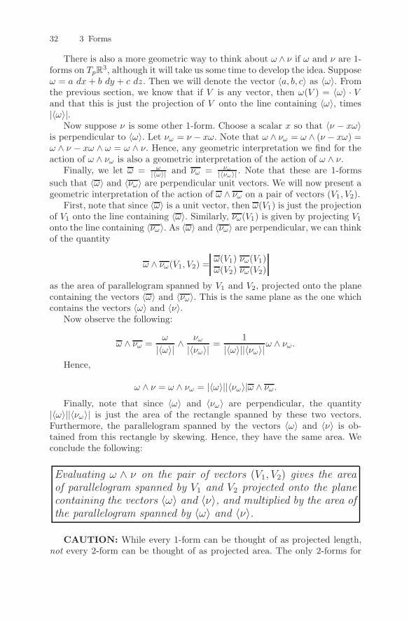
|〈ω〉||〈νω〉| is just the area of the rectangle spanned by these two vectors.Furthermore, the parallelogram spanned by the vectors 〈ω〉 and 〈ν〉 is ob-tained from this rectangle by skewing. Hence, they have the same area. Weconclude the following:
Evaluating ω ∧ ν on the pair of vectors (V1, V2) gives the areaof parallelogram spanned by V1 and V2 projected onto the planecontaining the vectors 〈ω〉 and 〈ν〉, and multiplied by the area ofthe parallelogram spanned by 〈ω〉 and 〈ν〉.
CAUTION: While every 1-form can be thought of as projected length,not every 2-form can be thought of as projected area. The only 2-forms for
3.3 Multiplying 1-forms 33
which this interpretation is valid are those that are the product of 1-forms.See Problem 3.18.
Let’s pause for a moment to look at a particularly simple 2-form on TpR3,
dx ∧ dy. Suppose V1 = 〈a1, a2, a3〉 and V2 = 〈b1, b2, b3〉. Then
dx ∧ dy(V1, V2) = a1 a2b1 b2
.
This is precisely the (signed) area of the parallelogram spanned by V1 and V2projected onto the dxdy-plane.
3.14. Show that for any 1-forms ω and ν on TR3, there are constants c1, c2,and c3 such that
ω ∧ ν = c1dx ∧ dy + c2dx ∧ dz + c3dy ∧ dz.The preceding comments and this last exercise give the following geometric
interpretation of the action of a 2-form on the pair of vectors (V1, V2):
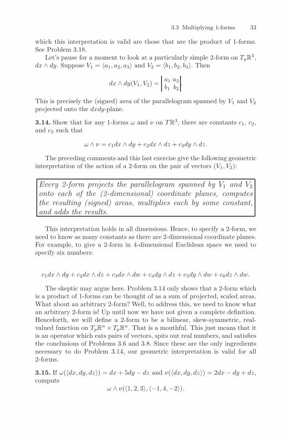
Every 2-form projects the parallelogram spanned by V1 and V2
onto each of the (2-dimensional) coordinate planes, computesthe resulting (signed) areas, multiplies each by some constant,and adds the results.
This interpretation holds in all dimensions. Hence, to specify a 2-form, weneed to know as many constants as there are 2-dimensional coordinate planes.For example, to give a 2-form in 4-dimensional Euclidean space we need tospecify six numbers:
c1dx ∧ dy + c2dx ∧ dz + c3dx ∧ dw + c4dy ∧ dz + c5dy ∧ dw + c6dz ∧ dw.The skeptic may argue here. Problem 3.14 only shows that a 2-form which
is a product of 1-forms can be thought of as a sum of projected, scaled areas.What about an arbitrary 2-form? Well, to address this, we need to know whatan arbitrary 2-form is! Up until now we have not given a complete definition.Henceforth, we will define a 2-form to be a bilinear, skew-symmetric, real-valued function on TpR
n×TpRn. That is a mouthful. This just means that it
is an operator which eats pairs of vectors, spits out real numbers, and satisfiesthe conclusions of Problems 3.6 and 3.8. Since these are the only ingredientsnecessary to do Problem 3.14, our geometric interpretation is valid for all2-forms.
3.15. If ω(〈dx, dy, dz〉) = dx+ 5dy − dz and ν(〈dx, dy, dz〉) = 2dx− dy + dz,compute
ω ∧ ν(〈1, 2, 3〉, 〈−1, 4,−2〉).
34 3 Forms
3.16. Let ω(〈dx, dy, dz〉) = dx+5dy−dz and ν(〈dx, dy, dz〉) = 2dx−dy+dz.Find constants c1, c2 and c3, such that
ω ∧ ν = c1dx ∧ dy + c2dy ∧ dz + c3dx ∧ dz.
3.17. Express each of the following as the product of two 1-forms:
1. 3dx ∧ dy + dy ∧ dx.2. dx ∧ dy + dx ∧ dz.3. 3dx ∧ dy + dy ∧ dx+ dx ∧ dz.4. dx ∧ dy + 3dz ∧ dy + 4dx ∧ dz.
3.4 2-Forms on TpR3 (optional)
This text is about differential n-forms on Rm. For most of it, we keep n,m ≤ 3
so that everything we do can be easily visualized. However, very little is specialabout these dimensions. Everything we do is presented so that it can easilygeneralize to higher dimensions. In this section and the next we break fromthis philosophy and present some special results when the dimensions involvedare 3 or 4.
3.18. Find a 2-form which is not the product of 1-forms.
In doing this exercise, you may guess that, in fact, all 2-forms on TpR3 can
be written as a product of 1-forms. Let’s see a proof of this fact that reliesheavily on the geometric interpretations we have developed.
Recall the correspondence introduced above between vectors and 1-forms.If α = a1dx+a2dy+a3dz, then we let 〈α〉 = 〈a1, a2, a3〉. If V is a vector, thenwe let 〈V 〉−1 be the corresponding 1-form.
We now prove two lemmas.
Lemma 1. If α and β are 1-forms on TpR3 and V is a vector in the plane
spanned by 〈α〉 and 〈β〉, then there is a vector, W , in this plane such thatα ∧ β = 〈V 〉−1 ∧ 〈W 〉−1.
Proof. The proof of the above lemma relies heavily on the fact that 2-formswhich are the product of 1-forms are very flexible. The 2-form α ∧ β takespairs of vectors, projects them onto the plane spanned by the vectors 〈α〉 and〈β〉, and computes the area of the resulting parallelogram times the area ofthe parallelogram spanned by 〈α〉 and 〈β〉. Note that for every nonzero scalarc, the area of the parallelogram spanned by 〈α〉 and 〈β〉 is the same as thearea of the parallelogram spanned by c〈α〉 and 1/c〈β〉. (This is the same thingas saying that α ∧ β = cα ∧ 1
cβ.) The important point here is that we canscale one of the 1-forms as much as we want at the expense of the other andget the same 2-form as a product.
3.4 2-Forms on TpR3 (optional) 35
Another thing we can do is apply a rotation to the pair of vectors 〈α〉and 〈β〉 in the plane which they determine. As the area of the parallelogramspanned by these two vectors is unchanged by rotation, their product stilldetermines the same 2-form. In particular, suppose V is any vector in theplane spanned by 〈α〉 and 〈β〉. Then we can rotate 〈α〉 and 〈β〉 to 〈α′〉 and〈β′〉 so that c〈α′〉 = V for some scalar c. We can then replace the pair (〈α〉, 〈β〉)with the pair (c〈α′〉, 1/c〈β′〉) = (V, 1/c〈β′〉). To complete the proof, let W =1/c〈β′〉.Lemma 2. If ω1 = α1∧β1 and ω2 = α2∧β2 are 2-forms on TpR
3, then thereexist 1-forms, α3 and β3, such that ω1 + ω2 = α3 ∧ β3.Proof. Let’s examine the sum α1 ∧ β1 + α2 ∧ β2. Our first case is that theplane spanned by the pair (〈α1〉, 〈β1〉) is the same as the plane spanned bythe pair (〈α2〉, 〈β2〉). In this case, it must be that α1 ∧ β1 = Cα2 ∧ β2 and,hence, α1 ∧ β1 + α2 ∧ β2 = (1 + C)α1 ∧ β1.
If these two planes are not the same, then they intersect in a line. Let Vbe a vector contained in this line. Then by the preceding lemma, there are1-forms γ and γ′ such that α1 ∧ β1 = 〈V 〉−1 ∧ γ and α2 ∧ β2 = 〈V 〉−1 ∧ γ′.Hence,
α1 ∧ β1 + α2 ∧ β2 = 〈V 〉−1 ∧ γ + 〈V 〉−1 ∧ γ′ = 〈V 〉−1 ∧ (γ + γ′).
Now note that any 2-form is the sum of products of 1-forms. Hence, thislast lemma implies that any 2-form on TpR
3 is a product of 1-forms. In otherwords:
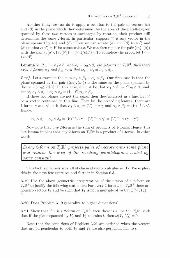
Every 2-form on TpR3 projects pairs of vectors onto some plane
and returns the area of the resulting parallelogram, scaled bysome constant.
This fact is precisely why all of classical vector calculus works. We explorethis in the next few exercises and further in Section 6.3.
3.19. Use the above geometric interpretation of the action of a 2-form onTpR
3 to justify the following statement: For every 2-form ω on TpR3 there are
nonzero vectors V1 and V2 such that V1 is not a multiple of V2 but ω(V1, V2) =0.
3.20. Does Problem 3.19 generalize to higher dimensions?
3.21. Show that if ω is a 2-form on TpR3, then there is a line l in TpR
3 suchthat if the plane spanned by V1 and V2 contains l, then ω(V1, V2) = 0.
Note that the conditions of Problem 3.21 are satisfied when the vectorsthat are perpendicular to both V1 and V2 are also perpendicular to l.
36 3 Forms
3.22. Show that if all you know about V1 and V2 is that they are vectorsin TpR
3 that span a parallelogram of area A, then the value of ω(V1, V2) ismaximized when V1 and V2 are perpendicular to the line l of Problem 3.21.
Note that the conditions of this exercise are satisfied when the vectorsperpendicular to V1 and V2 are parallel to l.
3.23. Let N be a vector perpendicular to V1 and V2 in TpR3 whose length is
precisely the area of the parallelogram spanned by these two vectors. Showthat there is a vector Vω in the line l of Problem 3.21 such that the value ofω(V1, V2) is precisely Vω ·N .
Remark. You may have learned that the vector N of the previous exerciseis precisely the cross product of V1 and V2. Hence, the previous problemimplies that if ω is a 2-form on TpR
3 then there is a vector Vω such thatω(V1, V2) = Vω · (V1 × V2).
3.24. Show that if ω = Fx dy ∧ dz − Fy dx ∧ dz + Fz dx ∧ dy, then Vω =〈Fx, Fy, Fz〉.
3.5 2-Forms and 3-forms on TpR4 (optional)
Many of the techniques of the previous section can be used to prove resultsabout 2- and 3-forms on TpR
4.
3.25. Show that any 3-form on TpR4 can be written as the product of three
1-forms. (Hint: Two 3-dimensional subspaces of TpR4 must meet in at least a
line.)
We now give away an answer to Problem 3.18. Let ω = dx∧ dy+ dz ∧ dw.Then an easy computation shows that ω ∧ ω = 2dx ∧ dy ∧ dz ∧ dw. However,if ω were equal to α ∧ β for some 1-forms α and β, then ω ∧ ω would be zero(why?). This argument shows that, in general, if ω is any 2-form such thatω ∧ ω = 0, then ω cannot be written as the product of 1-forms.
3.26. Let ω be a 2-form on TpR4. Show that ω can be written as the sum of
exactly two products; that is, ω = α ∧ β + δ ∧ γ. (Hint: Given three planes inTpR
4, there are at least two of them that intersect in more than a point.)
Above, we saw that if ω is a 2-form such that ω ∧ω = 0, then ω is not theproduct of 1-forms. We now use the previous exercise to show the converse.
Theorem 1. If ω is a 2-form on TpR4 such that ω ∧ ω = 0, then ω can be
written as the product of two 1-forms.
3.6 n-Forms 37
Our proof of this again relies heavily on the geometry of the situation. Bythe previous exercise, ω = α ∧ β + δ ∧ γ. A short computation then shows
ω ∧ ω = 2α ∧ β ∧ δ ∧ γ.If this 4-form is the zero 4-form, then it must be the case that the (4-
dimensional) volume of the parallelepiped spanned by 〈α〉, 〈β〉, 〈δ〉 and 〈γ〉is zero. This, in turn, implies that the plane spanned by 〈α〉 and 〈β〉 meetsthe plane spanned by 〈δ〉 and 〈γ〉 in at least a line (show this!). Call such anintersection line L.
As in the previous section, we can now rotate 〈α〉 and 〈β〉, in the planethey span, to vectors 〈α′〉 and 〈β′〉 such that 〈α′〉 lies in the line L. The 2-form α′ ∧ β′ must equal α ∧ β since they determine the same plane and spana parallelogram of the same area. Similarly, we rotate 〈δ〉 and 〈γ〉 to vectors〈δ′〉 and 〈γ′〉 such that 〈δ′〉 ⊂ L. It follows that δ ∧ γ = δ′ ∧ γ′.
Since 〈α′〉 and 〈δ′〉 lie on the same line, there is a constant c such thatcα′ = δ′. We now put all of this information together:
ω = α ∧ β + δ ∧ γ= α′ ∧ β′ + δ′ ∧ γ′
= (cα′) ∧(1
cβ′)+ δ′ ∧ γ′
= δ′ ∧(1
cβ′)+ δ′ ∧ γ′
= δ′ ∧(1
cβ′ + γ′
).
3.6 n-Forms
Let’s think a little more about our multiplication operator ∧. If it is reallygoing to be anything like multiplication, we should be able to take three 1-forms — ω, ν and ψ — and form the product ω ∧ ν ∧ ψ. How can we definethis? A first guess might be to say that ω ∧ ν ∧ ψ = ω ∧ (ν ∧ ψ), but ν ∧ ψ isa 2-form and we have not defined the product of a 2-form and a 1-form. Wetake a different approach and define ω ∧ ν ∧ ψ directly.
This is completely analogous to the previous section. ω, ν and ψ each acton a vector, V , to give three numbers. In other words, they can be thought ofas coordinate functions. We say the coordinates of V are [ω(V ), ν(V ), ψ(V )].Hence, if we have three vectors — V1, V2 and V3 — we can compute the[ω, ν, ψ] coordinates of each. This gives us three new vectors. The value ofω∧ν∧ψ(V1, V2, V3) is then defined to be the signed volume of the parallelepipedwhich they span.
There is no reason to stop at 3 dimensions. Suppose ω1, ω2, ..., ωn are 1-forms and V1, V2, ..., Vn are vectors. Then we define the value of
38 3 Forms
ω1 ∧ ω2 ∧ · · · ∧ ωn(V1, V2, ..., Vn)to be the signed (n-dimensional) volume of the parallelepiped spanned by thevectors [ω1(Vi), ω2(Vi), ..., ωn(Vi)]. Algebraically,
ω1 ∧ ω2 ∧ · · · ∧ ωn(V1, V2, ..., Vn) =ω1(V1) ω2(V1) · · · ωn(V1)ω1(V2) ω2(V2) · · · ωn(V2)
......
...ω1(Vn) ω2(Vn) · · · ωn(Vn)
3.27. Let γ be the 3-form 2dx ∧ dy ∧ dz. LetV1 = 〈1, 2, 1〉, V2 = 〈0, 1, 1〉, V3 = 〈−1,−2, 1〉.
Compute γ(V1, V2, V3).
3.28. Calculate α ∧ β ∧ γ(V1, V2, V3), whereα = dx+ 2dy + dz, β = dx− dz, γ = −dy + 3dz,
V1 = 〈1, 2, 3〉, V2 = 〈−1, 1, 1〉, V3 = 〈0, 1, 1〉.3.29. Note that, just as in Problem 3.12, if α, β and γ are 1-forms on TpR
3,then α∧β∧γ(V1, V2, V3) is the (signed) volume of the parallelepiped spannedby V1, V2 and V3 times the volume of the parallelepiped spanned by 〈α〉, 〈β〉and 〈γ〉. Suppose ω is a 2-form on TpR
3 and ν is a 1-form on TpR3. Show that
if ω∧ ν = 0, then there is a 1-form γ such that ω = ν ∧γ. (Hint: Combine thegiven geometric interpretation of a 3-form which is the product of 1-forms onTpR
3, with the results of Section 3.4.)
It follows from linear algebra that if we swap any two rows or columnsof this matrix, the sign of the result flips. Hence, if the n-tuple V′ =(Vi1 , Vi2 , ..., Vin) is obtained from V = (V1, V2, ..., Vn) by an even numberof exchanges, then the sign of ω1 ∧ ω2 ∧ · · · ∧ ωn(V′) will be the same as thesign of ω1∧ω2 ∧ · · ·∧ωn(V). If the number of exchanges is odd, then the signis opposite. We sum this up by saying that the n-form, ω1 ∧ ω2 ∧ · · · ∧ ωn isalternating.
The wedge product of 1-forms is also multilinear, in the following sense:
ω1 ∧ ω2 ∧ · · · ∧ ωn(V1, ..., Vi + V ′i , ..., Vn)
= ω1 ∧ ω2 ∧ · · · ∧ ωn(V1, ..., Vi, ..., Vn)+ω1 ∧ ω2 ∧ · · · ∧ ωn(V1, ..., V ′
i , ..., Vn)
and
ω1 ∧ ω2 ∧ · · · ∧ ωn(V1, ..., cVi, ..., Vn) = cω1 ∧ ω2 ∧ · · · ∧ ωn(V1, ..., Vi, ..., Vn)for all i and any real number c.
In general, we define an n-form to be any alternating, multilinear real-valued function which acts on n-tuples of vectors.
3.6 n-Forms 39
3.30. Prove the following geometric interpretation (Hint: All of the steps arecompletely analogous to those in Section 3.3.):
An m-form on TpRn can be thought of as a function which takes
the parallelepiped spanned by m vectors, projects it onto eachof the m-dimensional coordinate planes, computes the resultingareas, multiplies each by some constant, and adds the results.
3.31. How many numbers do you need to give to specify a 5-form on TpR10?
We turn now to the simple case of an n-form on TpRn. Notice that there
is only one n-dimensional coordinate plane in this space — namely the spaceitself. Such a form, evaluated on an n-tuple of vectors, must therefore give then-dimensional volume of the parallelepiped which it spans, multiplied by someconstant. For this reason, such a form is called a volume form (in 2-dimensions,an area form).
Example 14. Consider the forms, ω = dx + 2dy − dz, ν = 3dx − dy + dz andψ = −dx − 3dy + dz, on TpR
3. By the above argument, ω ∧ ν ∧ ψ must bea volume form. Which volume form is it? One way to tell is to compute itsvalue on a set of vectors which we know span a parallelepiped of volume one— namely 〈1, 0, 0〉, 〈0, 1, 0〉 and 〈0, 0, 1〉. This will tell us how much the formscales volume.
ω ∧ ν ∧ ψ(〈1, 0, 0〉, 〈0, 1, 0〉, 〈0, 0, 1〉) =1 3 −12 −1 −3
−1 1 1= 4.
So, ω ∧ ν ∧ ψ must be the same as the form 4dx ∧ dy ∧ dz.3.32. Let ω(〈dx, dy, dz〉) = dx+5dy−dz, ν(〈dx, dy, dz〉) = 2dx−dy+dz andγ(〈dx, dy, dz) = −dx+ dy + 2dz.
1. If V1 = 〈1, 0, 2〉, V2 = 〈1, 1, 2〉 and V3 = 〈0, 2, 3〉, compute ω ∧ ν ∧γ(V1, V2, V3).
2. Find a constant c such that ω ∧ ν ∧ γ = c dx ∧ dy ∧ dz.3. Let α = 3dx ∧ dy + 2dy ∧ dz − dx ∧ dz. Find a constant c such thatα ∧ γ = c dx ∧ dy ∧ dz.
3.33. Simplify
dx ∧ dy ∧ dz + dx ∧ dz ∧ dy + dy ∧ dz ∧ dx+ dy ∧ dx ∧ dy.3.34.
1. Expand and simplify
(dx + dy) ∧ (2dx+ dz) ∧ dz.
40 3 Forms
2. Plug the following vectors into the above 3-form:
V1 = 〈1, 1, 1〉, V2 = 〈1, 0, 1〉, V3 = 〈0, 1,−1〉3.35. Let ω be an n-form and ν an m-form.
1. Show thatω ∧ ν = (−1)nmν ∧ ω.
2. Use this to show that if n is odd, then ω ∧ ω = 0.
3.7 Algebraic computation of products
In this section, we break with the spirit of the text briefly. At this point,we have amassed enough algebraic identities that multiplying forms becomessimilar to multiplying polynomials. We quickly summarize these identities andwork a few examples.
Let ω be an n-form and ν be an m-form. Then we have the followingidentities:
ω ∧ ν = (−1)nmν ∧ ω,ω ∧ ω = 0 if n is odd,
ω ∧ (ν + ψ) = ω ∧ ν + ω ∧ ψ,(ν + ψ) ∧ ω = ν ∧ ω + ψ ∧ ω.
Example 15.
(x dx+ y dy) ∧ (y dx + x dy) =xy dx ∧ dx+ x2 dx ∧ dy + y2 dy ∧ dx+yx dy ∧ dy
= x2 dx ∧ dy + y2 dy ∧ dx= x2 dx ∧ dy − y2 dx ∧ dy= (x2 − y2) dx ∧ dy.
Example 16.
(x dx+ y dy) ∧ (xz dx ∧ dz + yz dy ∧ dz)=x2z dx ∧ dx ∧ dz + xyz dx ∧ dy ∧ dz+yxz dy ∧ dx ∧ dz +
y2z dy ∧ dy ∧ dz= xyz dx ∧ dy ∧ dz + yxz dy ∧ dx ∧ dz= xyz dx ∧ dy ∧ dz − xyz dx ∧ dy ∧ dz= 0.
3.36. Expand and simplify the following:
1. [(x− y) dx+ (x+ y) dy + z dz] ∧ [(x− y) dx+ (x+ y) dy].2. (2dx+ 3dy) ∧ (dx− dz) ∧ (dx + dy + dz).
4
Differential Forms
4.1 Families of forms
Let us now go back to the example in Chapter 1. In the last section of thatchapter, we showed that the integral of a function, f : R3 → R, over a surfaceparameterized by φ : R ⊂ R
2 → R3 is∫
R
f(φ(r, θ))Area
[∂φ
∂r(r, θ),
∂φ
∂θ(r, θ)
]dr dθ.
This gave one motivation for studying differential forms. We wanted togeneralize this integral by considering functions other than “Area(·, ·)” thateat pairs of vectors and return numbers. However, in this integral, the point atwhich such a pair of vectors is based changes. In other words, Area(·, ·) doesnot act on TpR
3 × TpR3 for a fixed p. We can make this point a little clearer
by reexamining the above integrand. Note that it is of the form f()Area(·, ·).For a fixed point, , of R3, this is an operator on TR
3 × TR3, much like a
2-form is.So far all we have done is to define 2-forms at fixed points of R3. To really
generalize the above integral, we must start to consider entire families of 2-forms, ωp : TpR
3 × TpR3 → R, where p ranges over all of R3. Of course, for
this to be useful, such a family must have some “niceness” properties. For onething, it should be continuous; that is, if p and q are close, then ωp and ωqshould be similar.
An even stronger property is that the family ωp is differentiable. To seewhat this means, recall that for a fixed p, a 2-form ωp can always be writtenas apdx ∧ dy+ bpdy ∧ dz + cpdx ∧ dz, where ap, bp and cp are constants. If welet our choice of p vary over all of R3, then so will these constants. In otherwords, ap, bp and cp are all functions from R
3 to R. To say that the family ωpis differentiable, we mean that each of these functions is differentiable. If ωpis differentiable, then we will refer to it as a differential form. When there canbe no confusion, we will suppress the subscript p.
DOI 10.1007/978-0-8176-830 - _4, © Springer Science+Business Media, LLC 2012, D. Bachman
4 741,A Geometric Approach to Differential Forms
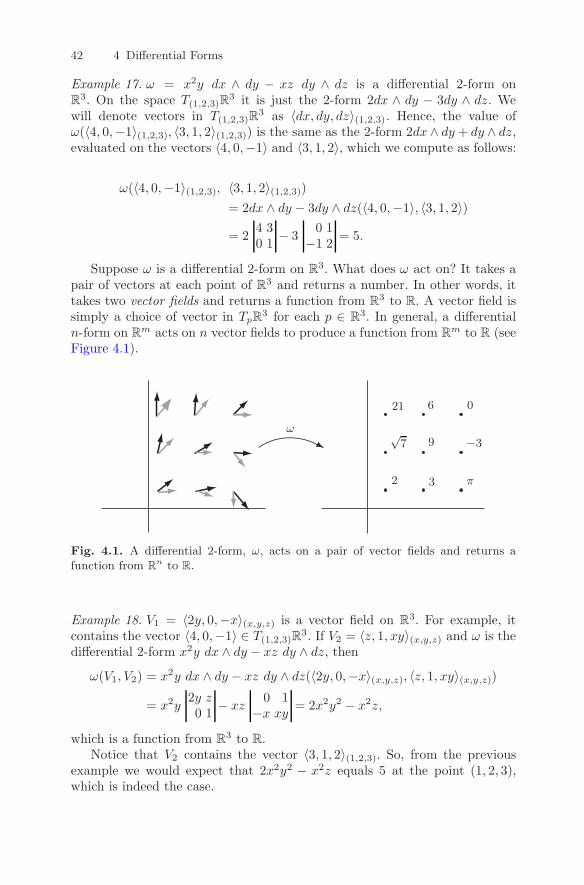
42 4 Differential Forms
Example 17. ω = x2y dx ∧ dy − xz dy ∧ dz is a differential 2-form onR
3. On the space T(1,2,3)R3 it is just the 2-form 2dx ∧ dy − 3dy ∧ dz. We
will denote vectors in T(1,2,3)R3 as 〈dx, dy, dz〉(1,2,3). Hence, the value of
ω(〈4, 0,−1〉(1,2,3), 〈3, 1, 2〉(1,2,3)) is the same as the 2-form 2dx ∧ dy+ dy ∧ dz,evaluated on the vectors 〈4, 0,−1〉 and 〈3, 1, 2〉, which we compute as follows:
ω(〈4, 0,−1〉(1,2,3), 〈3, 1, 2〉(1,2,3))= 2dx ∧ dy − 3dy ∧ dz(〈4, 0,−1〉, 〈3, 1, 2〉)= 2
4 30 1
− 30 1
−1 2= 5.
Suppose ω is a differential 2-form on R3. What does ω act on? It takes a
pair of vectors at each point of R3 and returns a number. In other words, ittakes two vector fields and returns a function from R
3 to R. A vector field issimply a choice of vector in TpR
3 for each p ∈ R3. In general, a differential
n-form on Rm acts on n vector fields to produce a function from R
m to R (seeFigure 4.1).
ω
2 3 π
√7 9 −3
21 6 0
Fig. 4.1. A differential 2-form, ω, acts on a pair of vector fields and returns afunction from R
n to R.
Example 18. V1 = 〈2y, 0,−x〉(x,y,z) is a vector field on R3. For example, it
contains the vector 〈4, 0,−1〉 ∈ T(1,2,3)R3. If V2 = 〈z, 1, xy〉(x,y,z) and ω is the
differential 2-form x2y dx ∧ dy − xz dy ∧ dz, thenω(V1, V2) = x2y dx ∧ dy − xz dy ∧ dz(〈2y, 0,−x〉(x,y,z), 〈z, 1, xy〉(x,y,z))
= x2y2y z0 1
− xz0 1
−x xy = 2x2y2 − x2z,
which is a function from R3 to R.
Notice that V2 contains the vector 〈3, 1, 2〉(1,2,3). So, from the previousexample we would expect that 2x2y2 − x2z equals 5 at the point (1, 2, 3),which is indeed the case.
4.2 Integrating differential 2-forms 43
4.1. Let ω be the differential 2-form on R3 given by
ω = xyz dx ∧ dy + x2z dy ∧ dz − y dx ∧ dz.
Let V1 and V2 be the following vector fields:
V1 = 〈y, z, x2〉(x,y,z), V2 = 〈xy, xz, y〉(x,y,z).
1. What vectors do V1 and V2 contain at the point (1, 2, 3)?2. Which 2-form is ω on T(1,2,3)R
3?3. Use your answers to the previous two questions to compute ω(V1, V2) at
the point (1, 2, 3).4. Compute ω(V1, V2) at the point (x, y, z). Then plug in x = 1, y = 2 andz = 3 to check your answer against the previous question.
4.2 Integrating differential 2-forms
Let’s now recall the steps involved with integration of functions on subsets ofR
2. Suppose R ⊂ R2 and f : R → R. The following steps define the integral
of f over R:
1. Choose a lattice of points in R, (xi, yj).2. For each i and j, define V 1
i,j = (xi+1, yj)− (xi, yj) and V2i,j = (xi, yj+1)−
(xi, yj) (see Figure 4.2). Notice that V 1i,j and V 2
i,j are both vectors in
T(xi,yj)R2.
3. For each i and j, compute f(xi, yj)Area(V1i,j , V
2i,j), where Area(V,W ) is
the function which returns the area of the parallelogram spanned by thevectors V and W .
4. Sum over all i and j.5. Take the limit as the maximal distance between adjacent lattice points
goes to zero. This is the number that we define to be the value of∫R
f dx dy.
Let’s focus on Step 3. Here we compute f(xi, yj)Area(V1i,j , V
2i,j). Notice
that this is exactly the value of the differential 2-form ω = f(x, y)dx ∧ dyevaluated on the vectors V 1
i,j and V2i,j at the point (xi, yj). Hence, in Step 4 we
can write this sum as∑i
∑j
f(xi, yj)Area(V1i,j , V
2i,j) =
∑i
∑j
ω(xi,yj)(V1i,j , V
2i,j).
It is reasonable, then, to adopt the shorthand “∫R
ω” to denote the limit in
Step 5. The upshot of all this is the following:
If ω = f(x, y)dx ∧ dy, then∫R
ω =∫R
f dx dy.
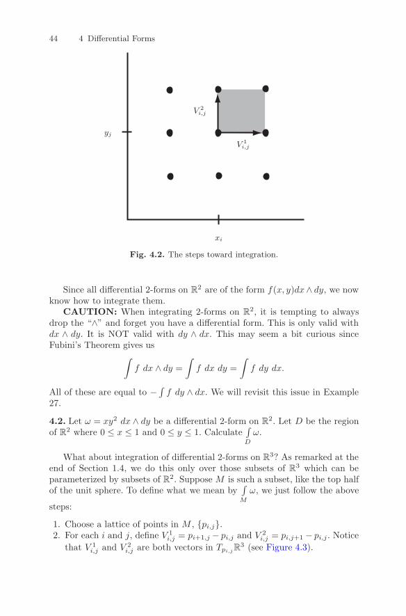
44 4 Differential Forms
xi
yj
V 1i,j
V 2i,j
Fig. 4.2. The steps toward integration.
Since all differential 2-forms on R2 are of the form f(x, y)dx∧ dy, we now
know how to integrate them.CAUTION: When integrating 2-forms on R
2, it is tempting to alwaysdrop the “∧” and forget you have a differential form. This is only valid withdx ∧ dy. It is NOT valid with dy ∧ dx. This may seem a bit curious sinceFubini’s Theorem gives us∫
f dx ∧ dy =
∫f dx dy =
∫f dy dx.
All of these are equal to − ∫f dy ∧ dx. We will revisit this issue in Example
27.
4.2. Let ω = xy2 dx ∧ dy be a differential 2-form on R2. Let D be the region
of R2 where 0 ≤ x ≤ 1 and 0 ≤ y ≤ 1. Calculate∫D
ω.
What about integration of differential 2-forms on R3? As remarked at the
end of Section 1.4, we do this only over those subsets of R3 which can beparameterized by subsets of R2. Suppose M is such a subset, like the top halfof the unit sphere. To define what we mean by
∫M
ω, we just follow the above
steps:
1. Choose a lattice of points in M , pi,j.2. For each i and j, define V 1
i,j = pi+1,j − pi,j and V2i,j = pi,j+1 − pi,j . Notice
that V 1i,j and V 2
i,j are both vectors in Tpi,jR3 (see Figure 4.3).
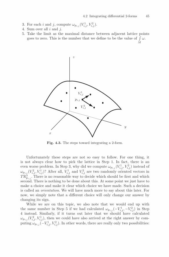
4.2 Integrating differential 2-forms 45
3. For each i and j, compute ωpi,j (V1i,j , V
2i,j).
4. Sum over all i and j.5. Take the limit as the maximal distance between adjacent lattice points
goes to zero. This is the number that we define to be the value of∫M
ω.
x
y
z
pi,j
V 1i,j
V 2i,j
Fig. 4.3. The steps toward integrating a 2-form.
Unfortunately these steps are not so easy to follow. For one thing, itis not always clear how to pick the lattice in Step 1. In fact, there is aneven worse problem. In Step 3, why did we compute ωpi,j (V
1i,j , V
2i,j) instead of
ωpi,j (V2i,j , V
1i,j)? After all, V 1
i,j and V 2i,j are two randomly oriented vectors in
TR3pi,j . There is no reasonable way to decide which should be first and which
second. There is nothing to be done about this. At some point we just have tomake a choice and make it clear which choice we have made. Such a decisionis called an orientation. We will have much more to say about this later. Fornow, we simply note that a different choice will only change our answer bychanging its sign.
While we are on this topic, we also note that we would end up withthe same number in Step 5 if we had calculated ωpi,j (−V 1
i,j ,−V 2i,j) in Step
4 instead. Similarly, if it turns out later that we should have calculatedωpi,j (V
2i,j , V
1i,j), then we could have also arrived at the right answer by com-
puting ωpi,j (−V 1i,j , V
2i,j). In other words, there are really only two possibilities:
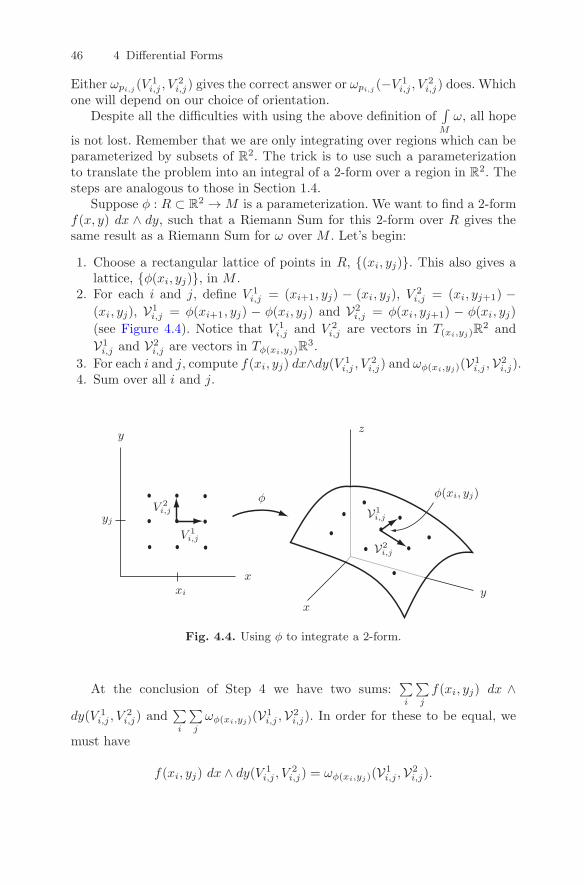
46 4 Differential Forms
Either ωpi,j (V1i,j , V
2i,j) gives the correct answer or ωpi,j (−V 1
i,j , V2i,j) does. Which
one will depend on our choice of orientation.Despite all the difficulties with using the above definition of
∫M
ω, all hope
is not lost. Remember that we are only integrating over regions which can beparameterized by subsets of R2. The trick is to use such a parameterizationto translate the problem into an integral of a 2-form over a region in R
2. Thesteps are analogous to those in Section 1.4.
Suppose φ : R ⊂ R2 →M is a parameterization. We want to find a 2-form
f(x, y) dx ∧ dy, such that a Riemann Sum for this 2-form over R gives thesame result as a Riemann Sum for ω over M . Let’s begin:
1. Choose a rectangular lattice of points in R, (xi, yj). This also gives alattice, φ(xi, yj), in M .
2. For each i and j, define V 1i,j = (xi+1, yj) − (xi, yj), V
2i,j = (xi, yj+1) −
(xi, yj), V1i,j = φ(xi+1, yj) − φ(xi, yj) and V2
i,j = φ(xi, yj+1) − φ(xi, yj)
(see Figure 4.4). Notice that V 1i,j and V 2
i,j are vectors in T(xi,yj)R2 and
V1i,j and V2
i,j are vectors in Tφ(xi,yj)R3.
3. For each i and j, compute f(xi, yj) dx∧dy(V 1i,j , V
2i,j) and ωφ(xi,yj)(V1
i,j ,V2i,j).
4. Sum over all i and j.
x
x
y
y
z
φ
xi
yj V1i,j
V2i,j
φ(xi, yj)
V 1i,j
V 2i,j
Fig. 4.4. Using φ to integrate a 2-form.
At the conclusion of Step 4 we have two sums:∑i
∑j
f(xi, yj) dx ∧dy(V 1
i,j , V2i,j) and
∑i
∑j
ωφ(xi,yj)(V1i,j ,V2
i,j). In order for these to be equal, we
must have
f(xi, yj) dx ∧ dy(V 1i,j , V
2i,j) = ωφ(xi,yj)(V1
i,j ,V2i,j).
4.2 Integrating differential 2-forms 47
So,
f(xi, yj) =ωφ(xi,yj)(V1
i,j ,V2i,j)
dx ∧ dy(V 1i,j , V
2i,j)
.
Since we are using a rectangular lattice in R, we know dx ∧ dy(V 1i,j , V
2i,j) =
Area(V 1i,j , V
2i,j) = |V 1
i,j | · |V 2i,j |. We now have
f(xi, yj) =ωφ(xi,yj)(V1
i,j ,V2i,j)
|V 1i,j | · |V 2
i,j |.
Using the bilinearity of ω, this reduces to
f(xi, yj) = ωφ(xi,yj)
(V1i,j
|V 1i,j |
,V2i,j
|V 2i,j |
).
As the distance between adjacent points of our partition tends toward zero,
V1i,j
|V 1i,j |
=φ(xi+1, yj)− φ(xi, yj)
|(xi+1, yj)− (xi, yj)| =φ(xi+1, yj)− φ(xi, yj)
|xi+1 − xi| → ∂φ
∂x(xi, yj).
Similarly,V2
i,j
|V 2i,j | converges to
∂φ∂y (xi, yj).
Let’s summarize what we have so far. We defined f(x, y) so that∑i
∑j
ωφ(xi,yj)(V1i,j ,V2
i,j)
=∑i
∑j
f(xi, yj) dx ∧ dy(V 1i,j , V
2i,j)
=∑i
∑j
ωφ(xi,yj)
(V1i,j
|V 1i,j |
,V2i,j
|V 2i,j |
)dx ∧ dy(V 1
i,j , V2i,j).
We have also shown that when we take the limit as the distance betweenadjacent partition points tends toward zero, this sum converges to the sum
∑i
∑j
ωφ(x,y)
(∂φ
∂x(x, y),
∂φ
∂y(x, y)
)dx ∧ dy(V 1
i,j , V2i,j).
Hence, it must be that
∫M
ω =
∫R
ωφ(x,y)
(∂φ
∂x(x, y),
∂φ
∂y(x, y)
)dx ∧ dy. (4.1)
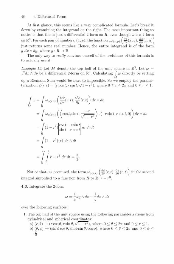
48 4 Differential Forms
At first glance, this seems like a very complicated formula. Let’s break itdown by examining the integrand on the right. The most important thing tonotice is that this is just a differential 2-form on R, even though ω is a 2-form
onR3. For each pair of numbers, (x, y), the function ωφ(x,y)
(∂φ∂x (x, y),
∂φ∂y (x, y)
)just returns some real number. Hence, the entire integrand is of the formg dx ∧ dy, where g : R→ R.
The only way to really convince oneself of the usefulness of this formula isto actually use it.
Example 19. Let M denote the top half of the unit sphere in R3. Let ω =
z2dx ∧ dy be a differential 2-form on R3. Calculating
∫M
ω directly by setting
up a Riemann Sum would be next to impossible. So we employ the parame-terization φ(r, t) = (r cos t, r sin t,
√1− r2), where 0 ≤ t ≤ 2π and 0 ≤ r ≤ 1.
∫M
ω =
∫R
ωφ(r,t)
(∂φ
∂r(r, t),
∂φ
∂t(r, t)
)dr ∧ dt
=
∫R
ωφ(r,t)
(⟨cos t, sin t,
−r√1− r2
⟩, 〈−r sin t, r cos t, 0〉
)dr ∧ dt
=
∫R
(1− r2)cos t −r sin tsin t r cos t
dr ∧ dt
=
∫R
(1− r2)(r) dr ∧ dt
=
2π∫0
1∫0
r − r3 dr dt =π
2.
Notice that, as promised, the term ωφ(r,t)
(∂φ∂r (r, t),
∂φ∂t (r, t)
)in the second
integral simplified to a function from R to R: r − r3.
4.3. Integrate the 2-form
ω =1
xdy ∧ dz − 1
ydx ∧ dz
over the following surfaces:
1. The top half of the unit sphere using the following parameterizations fromcylindrical and spherical coordinates:a) (r, θ) → (r cos θ, r sin θ,
√1− r2), where 0 ≤ θ ≤ 2π and 0 ≤ r ≤ 1.
b) (θ, φ) → (sinφ cos θ, sinφ sin θ, cosφ), where 0 ≤ θ ≤ 2π and 0 ≤ φ ≤π2 .
4.2 Integrating differential 2-forms 49
2. The surface parameterized by
φ(r, θ) = (r cos θ, r sin θ, cos r), 0 ≤ r ≤ π
2, 0 ≤ θ ≤ 2π.
3. The surface parameterized by
Ψ(θ, φ) = (cosφ cos θ, cosφ sin θ, sinφ), 0 ≤ θ ≤ 2π, −π4≤ φ ≤ π
4.
4.4. Let S be the surface in R3 parameterized by
Ψ(θ, z) = (cos θ, sin θ, z),
where 0 ≤ θ ≤ π and 0 ≤ z ≤ 1. Let ω = xyz dy ∧ dz. Calculate ∫S
ω.
4.5. Let ω be the differential 2-form on R3 given by
ω = xyz dx ∧ dy + x2z dy ∧ dz − y dx ∧ dz.1. Let P be the portion of the plane 3 = 2x + 3y − z in R
3 that lies abovethe square (x, y)|0 ≤ x ≤ 1, 0 ≤ y ≤ 1. Calculate ∫
P
ω.
2. Let M be the portion of the graph of z = x2 + y2 in R3 that lies above
the rectangle (x, y)|0 ≤ x ≤ 1, 0 ≤ y ≤ 2. Calculate ∫M
ω.
4.6. Let S be the surface given by the parameterization
φ(r, θ) = (r cos θ, r sin θ,√r2 + 1), 0 ≤ r ≤ 1, 0 ≤ θ ≤ π
2.
Let ω be the differential 2-form given by
ω = xz dx ∧ dz − yz dy ∧ dz.Compute
∫S
ω.
4.7. Let S be the surface in R3 parameterized by
Ψ(u, v) = (2u, v, u2 + v3), 0 ≤ u ≤ 1, 0 ≤ v ≤ 2.
Integrate the 2-form (x+ 2y) dx ∧ dz over S.
4.8. Let D be some region in the xy-plane. Let M denote the portion of thegraph of z = g(x, y) that lies above D.
1. Let ω = f(x, y) dx ∧ dy be a differential 2-form on R3. Show that∫
M
ω =
∫D
f(x, y) dx dy.
Notice the answer does not depend on the function g(x, y).
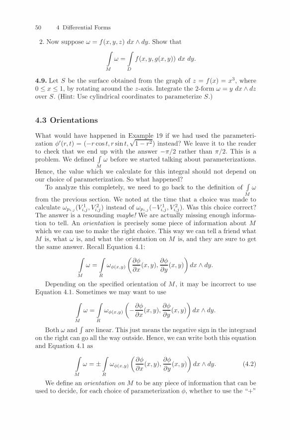
50 4 Differential Forms
2. Now suppose ω = f(x, y, z) dx ∧ dy. Show that∫M
ω =
∫D
f(x, y, g(x, y)) dx dy.
4.9. Let S be the surface obtained from the graph of z = f(x) = x3, where0 ≤ x ≤ 1, by rotating around the z-axis. Integrate the 2-form ω = y dx ∧ dzover S. (Hint: Use cylindrical coordinates to parameterize S.)
4.3 Orientations
What would have happened in Example 19 if we had used the parameteri-zation φ′(r, t) = (−r cos t, r sin t,√1− r2) instead? We leave it to the readerto check that we end up with the answer −π/2 rather than π/2. This is aproblem. We defined
∫M
ω before we started talking about parameterizations.
Hence, the value which we calculate for this integral should not depend onour choice of parameterization. So what happened?
To analyze this completely, we need to go back to the definition of∫M
ω
from the previous section. We noted at the time that a choice was made tocalculate ωpi,j (V
1i,j , V
2i,j) instead of ωpi,j (−V 1
i,j , V2i,j). Was this choice correct?
The answer is a resounding maybe! We are actually missing enough informa-tion to tell. An orientation is precisely some piece of information about Mwhich we can use to make the right choice. This way we can tell a friend whatM is, what ω is, and what the orientation on M is, and they are sure to getthe same answer. Recall Equation 4.1:∫
M
ω =
∫R
ωφ(x,y)
(∂φ
∂x(x, y),
∂φ
∂y(x, y)
)dx ∧ dy.
Depending on the specified orientation of M , it may be incorrect to useEquation 4.1. Sometimes we may want to use∫
M
ω =
∫R
ωφ(x,y)
(−∂φ∂x
(x, y),∂φ
∂y(x, y)
)dx ∧ dy.
Both ω and∫are linear. This just means the negative sign in the integrand
on the right can go all the way outside. Hence, we can write both this equationand Equation 4.1 as∫
M
ω = ±∫R
ωφ(x,y)
(∂φ
∂x(x, y),
∂φ
∂y(x, y)
)dx ∧ dy. (4.2)
We define an orientation on M to be any piece of information that can beused to decide, for each choice of parameterization φ, whether to use the “+”
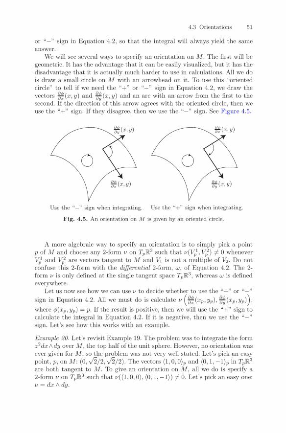
4.3 Orientations 51
or “−” sign in Equation 4.2, so that the integral will always yield the sameanswer.
We will see several ways to specify an orientation on M . The first will begeometric. It has the advantage that it can be easily visualized, but it has thedisadvantage that it is actually much harder to use in calculations. All we dois draw a small circle on M with an arrowhead on it. To use this “orientedcircle” to tell if we need the “+” or “−” sign in Equation 4.2, we draw thevectors ∂φ
∂x (x, y) and∂φ∂y (x, y) and an arc with an arrow from the first to the
second. If the direction of this arrow agrees with the oriented circle, then weuse the “+” sign. If they disagree, then we use the “−” sign. See Figure 4.5.
∂φ∂x
(x, y)
∂φ∂x
(x, y) ∂φ∂y
(x, y)
∂φ∂y
(x, y)
Use the “−” sign when integrating. Use the “+” sign when integrating.
Fig. 4.5. An orientation on M is given by an oriented circle.
A more algebraic way to specify an orientation is to simply pick a pointp of M and choose any 2-form ν on TpR
3 such that ν(V 1p , V
2p ) = 0 whenever
V 1p and V 2
p are vectors tangent to M and V1 is not a multiple of V2. Do notconfuse this 2-form with the differential 2-form, ω, of Equation 4.2. The 2-form ν is only defined at the single tangent space TpR
3, whereas ω is definedeverywhere.
Let us now see how we can use ν to decide whether to use the “+” or “−”
sign in Equation 4.2. All we must do is calculate ν(∂φ∂x (xp, yp),
∂φ∂y (xp, yp)
),
where φ(xp, yp) = p. If the result is positive, then we will use the “+” sign tocalculate the integral in Equation 4.2. If it is negative, then we use the “−”sign. Let’s see how this works with an example.
Example 20. Let’s revisit Example 19. The problem was to integrate the formz2dx∧dy overM , the top half of the unit sphere. However, no orientation wasever given for M , so the problem was not very well stated. Let’s pick an easypoint, p, on M : (0,
√2/2,
√2/2). The vectors 〈1, 0, 0〉p and 〈0, 1,−1〉p in TpR3
are both tangent to M . To give an orientation on M , all we do is specify a2-form ν on TpR
3 such that ν(〈1, 0, 0〉, 〈0, 1,−1〉) = 0. Let’s pick an easy one:ν = dx ∧ dy.
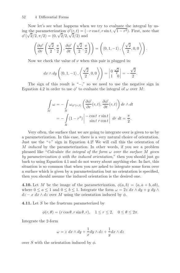
52 4 Differential Forms
Now let’s see what happens when we try to evaluate the integral by us-ing the parameterization φ′(r, t) = (−r cos t, r sin t,√1− r2). First, note thatφ′(
√2/2, π/2) = (0,
√2/2,
√2/2) and(
∂φ′
∂r
(√2
2,π
2
),∂φ′
∂t
(√2
2,π
2
))=
(〈0, 1,−1〉 ,
⟨√2
2, 0, 0
⟩).
Now we check the value of ν when this pair is plugged in:
dx ∧ dy(〈0, 1,−1〉 ,
⟨√2
2, 0, 0
⟩)=
∣∣∣∣0√22
1 0
∣∣∣∣ = −√2
2.
The sign of this result is “−,” so we need to use the negative sign inEquation 4.2 in order to use φ′ to evaluate the integral of ω over M :
∫M
ω = −∫R
ωφ′(r,t)
(∂φ′
∂r(r, t),
∂φ′
∂t(r, t)
)dr ∧ dt
= −∫R
(1− r2)
∣∣∣∣− cos t r sin tsin t r cos t
∣∣∣∣ dr dt = π
2.
Very often, the surface that we are going to integrate over is given to us bya parameterization. In this case, there is a very natural choice of orientation.Just use the “+” sign in Equation 4.2! We will call this the orientation ofM induced by the parameterization. In other words, if you see a problemphrased like “Calculate the integral of the form ω over the surface M givenby parameterization φ with the induced orientation,” then you should just goback to using Equation 4.1 and do not worry about anything else. In fact, thissituation is so common that when you are asked to integrate some form overa surface which is given by a parameterization but no orientation is specified,then you should assume the induced orientation is the desired one.
4.10. Let M be the image of the parameterization, φ(a, b) = (a, a + b, ab),where 0 ≤ a ≤ 1 and 0 ≤ b ≤ 1. Integrate the form ω = 2z dx ∧ dy + y dy ∧dz − x dx ∧ dz over M using the orientation induced by φ.
4.11. Let S be the frustrum parameterized by
φ(r, θ) = (r cos θ, r sin θ, r), 1 ≤ r ≤ 2, 0 ≤ θ ≤ 2π.
Integrate the 2-form
ω = z dx ∧ dy + 1
xdy ∧ dz + 1
ydx ∧ dz
over S with the orientation induced by φ.
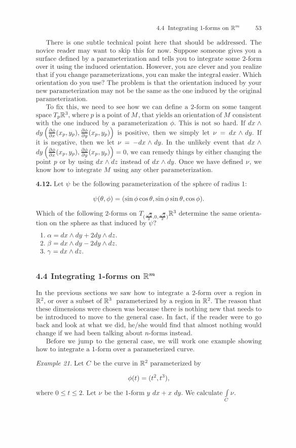
4.4 Integrating 1-forms on Rm 53
There is one subtle technical point here that should be addressed. Thenovice reader may want to skip this for now. Suppose someone gives you asurface defined by a parameterization and tells you to integrate some 2-formover it using the induced orientation. However, you are clever and you realizethat if you change parameterizations, you can make the integral easier. Whichorientation do you use? The problem is that the orientation induced by yournew parameterization may not be the same as the one induced by the originalparameterization.
To fix this, we need to see how we can define a 2-form on some tangentspace TpR
3, where p is a point ofM , that yields an orientation ofM consistentwith the one induced by a parameterization φ. This is not so hard. If dx ∧dy
(∂φ∂x (xp, yp),
∂φ∂y (xp, yp)
)is positive, then we simply let ν = dx ∧ dy. If
it is negative, then we let ν = −dx ∧ dy. In the unlikely event that dx ∧dy
(∂φ∂x (xp, yp),
∂φ∂y (xp, yp)
)= 0, we can remedy things by either changing the
point p or by using dx ∧ dz instead of dx ∧ dy. Once we have defined ν, weknow how to integrate M using any other parameterization.
4.12. Let ψ be the following parameterization of the sphere of radius 1:
ψ(θ, φ) = (sinφ cos θ, sinφ sin θ, cosφ).
Which of the following 2-forms on T(√
22 ,0,
√2
2 )R
3 determine the same orienta-
tion on the sphere as that induced by ψ?
1. α = dx ∧ dy + 2dy ∧ dz.2. β = dx ∧ dy − 2dy ∧ dz.3. γ = dx ∧ dz.
4.4 Integrating 1-forms on Rm
In the previous sections we saw how to integrate a 2-form over a region inR
2, or over a subset of R3 parameterized by a region in R2. The reason that
these dimensions were chosen was because there is nothing new that needs tobe introduced to move to the general case. In fact, if the reader were to goback and look at what we did, he/she would find that almost nothing wouldchange if we had been talking about n-forms instead.
Before we jump to the general case, we will work one example showinghow to integrate a 1-form over a parameterized curve.
Example 21. Let C be the curve in R2 parameterized by
φ(t) = (t2, t3),
where 0 ≤ t ≤ 2. Let ν be the 1-form y dx+ x dy. We calculate∫C
ν.
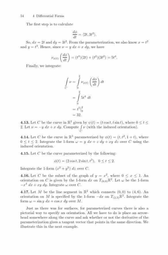
54 4 Differential Forms
The first step is to calculate
dφ
dt= 〈2t, 3t2〉.
So, dx = 2t and dy = 3t2. From the parameterization, we also know x = t2
and y = t3. Hence, since ν = y dx+ x dy, we have
νφ(t)
(dφ
dt
)= (t3)(2t) + (t2)(3t2) = 5t4.
Finally, we integrate:
∫C
ν =
2∫0
νφ(t)
(dφ
dt
)dt
=
2∫0
5t4 dt
= t5∣∣20
= 32.
4.13. Let C be the curve in R2 given by ψ(t) = (t cos t, t sin t), where 0 ≤ t ≤
2. Let ν = −y dx+ x dy. Compute∫C
ν (with the induced orientation).
4.14. Let C be the curve in R3 parameterized by φ(t) = (t, t2, 1 + t), where
0 ≤ t ≤ 2. Integrate the 1-form ω = y dx + z dy + xy dz over C using theinduced orientation.
4.15. Let C be the curve parameterized by the following:
φ(t) = (2 cos t, 2 sin t, t2), 0 ≤ t ≤ 2.
Integrate the 1-form (x2 + y2) dz over C.
4.16. Let C be the subset of the graph of y = x2, where 0 ≤ x ≤ 1. Anorientation on C is given by the 1-form dx on T(0,0)R
2. Let ω be the 1-form−x4 dx+ xy dy. Integrate ω over C.
4.17. Let M be the line segment in R2 which connects (0, 0) to (4, 6). An
orientation on M is specified by the 1-form −dx on T(2,3)R2. Integrate the
form ω = sin y dx+ cosx dy over M .
Just as there was for surfaces, for parameterized curves there is also apictorial way to specify an orientation. All we have to do is place an arrow-head somewhere along the curve and ask whether or not the derivative of theparameterization gives a tangent vector that points in the same direction. Weillustrate this in the next example.
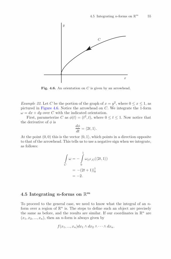
4.5 Integrating n-forms on Rm 55
x
y
C
Fig. 4.6. An orientation on C is given by an arrowhead.
Example 22. Let C be the portion of the graph of x = y2, where 0 ≤ x ≤ 1, aspictured in Figure 4.6. Notice the arrowhead on C. We integrate the 1-formω = dx+ dy over C with the indicated orientation.
First, parameterize C as φ(t) = (t2, t), where 0 ≤ t ≤ 1. Now notice thatthe derivative of φ is
dφ
dt= 〈2t, 1〉.
At the point (0, 0) this is the vector 〈0, 1〉, which points in a direction oppositeto that of the arrowhead. This tells us to use a negative sign when we integrate,as follows:
∫C
ω = −1∫
0
ω(t2,t)(〈2t, 1〉)
= −(2t+ 1)|10= −2.
4.5 Integrating n-forms on Rm
To proceed to the general case, we need to know what the integral of an n-form over a region of Rn is. The steps to define such an object are preciselythe same as before, and the results are similar. If our coordinates in R
n are(x1, x2, ..., xn), then an n-form is always given by
f(x1, ..., xn)dx1 ∧ dx2 ∧ · · · ∧ dxn.
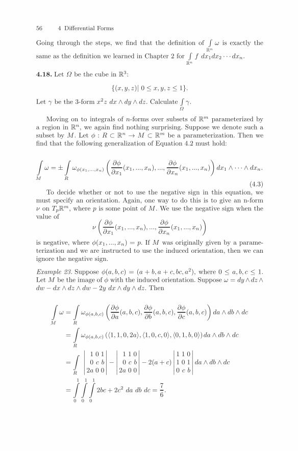
56 4 Differential Forms
Going through the steps, we find that the definition of∫Rn
ω is exactly the
same as the definition we learned in Chapter 2 for∫Rn
f dx1dx2 · · · dxn.
4.18. Let Ω be the cube in R3:
(x, y, z)| 0 ≤ x, y, z ≤ 1.Let γ be the 3-form x2z dx ∧ dy ∧ dz. Calculate ∫
Ω
γ.
Moving on to integrals of n-forms over subsets of Rm parameterized bya region in R
n, we again find nothing surprising. Suppose we denote such asubset by M . Let φ : R ⊂ R
n → M ⊂ Rm be a parameterization. Then we
find that the following generalization of Equation 4.2 must hold:
∫M
ω = ±∫R
ωφ(x1,...,xn)
(∂φ
∂x1(x1, ..., xn), ...,
∂φ
∂xn(x1, ..., xn)
)dx1 ∧ · · · ∧ dxn.
(4.3)To decide whether or not to use the negative sign in this equation, we
must specify an orientation. Again, one way to do this is to give an n-formν on TpR
m, where p is some point of M . We use the negative sign when thevalue of
ν
(∂φ
∂x1(x1, ..., xn), ...,
∂φ
∂xn(x1, ..., xn)
)is negative, where φ(x1, ..., xn) = p. If M was originally given by a parame-terization and we are instructed to use the induced orientation, then we canignore the negative sign.
Example 23. Suppose φ(a, b, c) = (a + b, a + c, bc, a2), where 0 ≤ a, b, c ≤ 1.LetM be the image of φ with the induced orientation. Suppose ω = dy∧dz∧dw − dx ∧ dz ∧ dw − 2y dx ∧ dy ∧ dz. Then
∫M
ω =
∫R
ωφ(a,b,c)
(∂φ
∂a(a, b, c),
∂φ
∂b(a, b, c),
∂φ
∂c(a, b, c)
)da ∧ db ∧ dc
=
∫R
ωφ(a,b,c) (〈1, 1, 0, 2a〉, 〈1, 0, c, 0〉, 〈0, 1, b, 0〉)da ∧ db ∧ dc
=
∫R
∣∣∣∣∣∣1 0 10 c b
2a 0 0
∣∣∣∣∣∣−∣∣∣∣∣∣
1 1 00 c b
2a 0 0
∣∣∣∣∣∣− 2(a+ c)
∣∣∣∣∣∣1 1 01 0 10 c b
∣∣∣∣∣∣ da ∧ db ∧ dc
=
1∫0
1∫0
1∫0
2bc+ 2c2 da db dc =7
6.
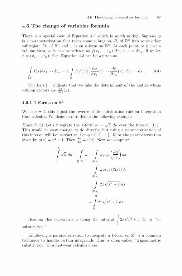
4.6 The change of variables formula 57
4.6 The change of variables formula
There is a special case of Equation 4.3 which is worth noting. Suppose φis a parameterization that takes some subregion, R, of Rn into some othersubregion, M , of Rn and ω is an n-form on R
n. At each point, ω is just avolume form, so it can be written as f(x1, ..., xn) dx1 ∧ · · · ∧ dxn. If we letx = (x1, ..., xn), then Equation 4.3 can be written as
∫M
f(x)dx1 · · · dxn = ±∫R
f(φ(x))
∣∣∣∣ ∂φ∂x1 (x) · · ·∂φ
∂xn(x)
∣∣∣∣ dx1 · · · dxn. (4.4)
The bars | · | indicate that we take the determinant of the matrix whosecolumn vectors are ∂φ
∂xi(x).
4.6.1 1-Forms on R1
When n = 1, this is just the reverse of the substitution rule for integrationfrom calculus. We demonstrate this in the following example.
Example 24. Let’s integrate the 1-form ω =√u du over the interval [1, 5].
This would be easy enough to do directly, but using a parameterization ofthis interval will be instructive. Let φ : [0, 2] → [1, 5] be the parameterizationgiven by φ(x) = x2 + 1. Then dφ
dx = 〈2x〉. Now we compute:
5∫1
√u du =
∫[1,5]
ω =
∫[0,2]
ωφ(x)
(dφ
dx
)dx
=
∫[0,2]
ωx2+1 (〈2x〉) dx
=
∫[0,2]
2x√x2 + 1 dx
=
2∫0
2x√x2 + 1 dx.
Reading this backwards is doing the integral2∫0
2x√x2 + 1 dx by “u-
substitution.”
Employing a parameterization to integrate a 1-form on R1 is a common
technique to handle certain integrands. This is often called “trigonometricsubstitution” in a first-year calculus class.
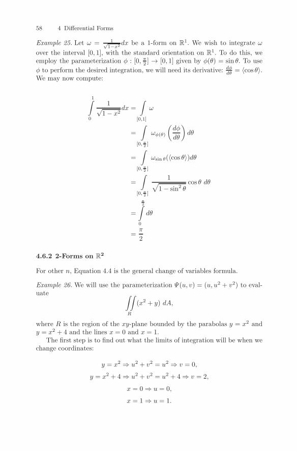
58 4 Differential Forms
Example 25. Let ω = 1√1−x2
dx be a 1-form on R1. We wish to integrate ω
over the interval [0, 1], with the standard orientation on R1. To do this, we
employ the parameterization φ : [0, π2 ] → [0, 1] given by φ(θ) = sin θ. To use
φ to perform the desired integration, we will need its derivative: dφdθ = 〈cos θ〉.We may now compute:
1∫0
1√1− x2
dx =
∫[0,1]
ω
=
∫[0,π2 ]
ωφ(θ)
(dφ
dθ
)dθ
=
∫[0,π2 ]
ωsin θ(〈cos θ〉)dθ
=
∫[0,π2 ]
1√1− sin2 θ
cos θ dθ
=
π2∫
0
dθ
=π
2
4.6.2 2-Forms on R2
For other n, Equation 4.4 is the general change of variables formula.
Example 26. We will use the parameterization Ψ(u, v) = (u, u2 + v2) to eval-uate ∫∫
R
(x2 + y) dA,
where R is the region of the xy-plane bounded by the parabolas y = x2 andy = x2 + 4 and the lines x = 0 and x = 1.
The first step is to find out what the limits of integration will be when wechange coordinates:
y = x2 ⇒ u2 + v2 = u2 ⇒ v = 0,
y = x2 + 4 ⇒ u2 + v2 = u2 + 4 ⇒ v = 2,
x = 0 ⇒ u = 0,
x = 1 ⇒ u = 1.
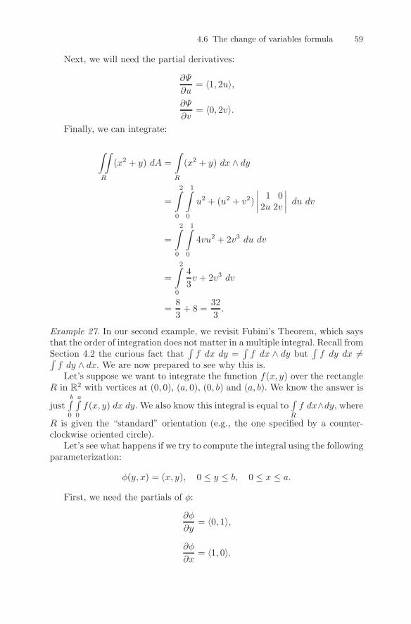
4.6 The change of variables formula 59
Next, we will need the partial derivatives:
∂Ψ
∂u= 〈1, 2u〉,
∂Ψ
∂v= 〈0, 2v〉.
Finally, we can integrate:
∫∫R
(x2 + y) dA =
∫R
(x2 + y) dx ∧ dy
=
2∫0
1∫0
u2 + (u2 + v2)
∣∣∣∣ 1 02u 2v
∣∣∣∣ du dv
=
2∫0
1∫0
4vu2 + 2v3 du dv
=
2∫0
4
3v + 2v3 dv
=8
3+ 8 =
32
3.
Example 27. In our second example, we revisit Fubini’s Theorem, which saysthat the order of integration does not matter in a multiple integral. Recall fromSection 4.2 the curious fact that
∫f dx dy =
∫f dx ∧ dy but
∫f dy dx =∫
f dy ∧ dx. We are now prepared to see why this is.Let’s suppose we want to integrate the function f(x, y) over the rectangle
R in R2 with vertices at (0, 0), (a, 0), (0, b) and (a, b). We know the answer is
justb∫0
a∫0
f(x, y) dx dy. We also know this integral is equal to∫R
f dx∧dy, whereR is given the “standard” orientation (e.g., the one specified by a counter-clockwise oriented circle).
Let’s see what happens if we try to compute the integral using the followingparameterization:
φ(y, x) = (x, y), 0 ≤ y ≤ b, 0 ≤ x ≤ a.
First, we need the partials of φ:
∂φ
∂y= 〈0, 1〉,
∂φ
∂x= 〈1, 0〉.
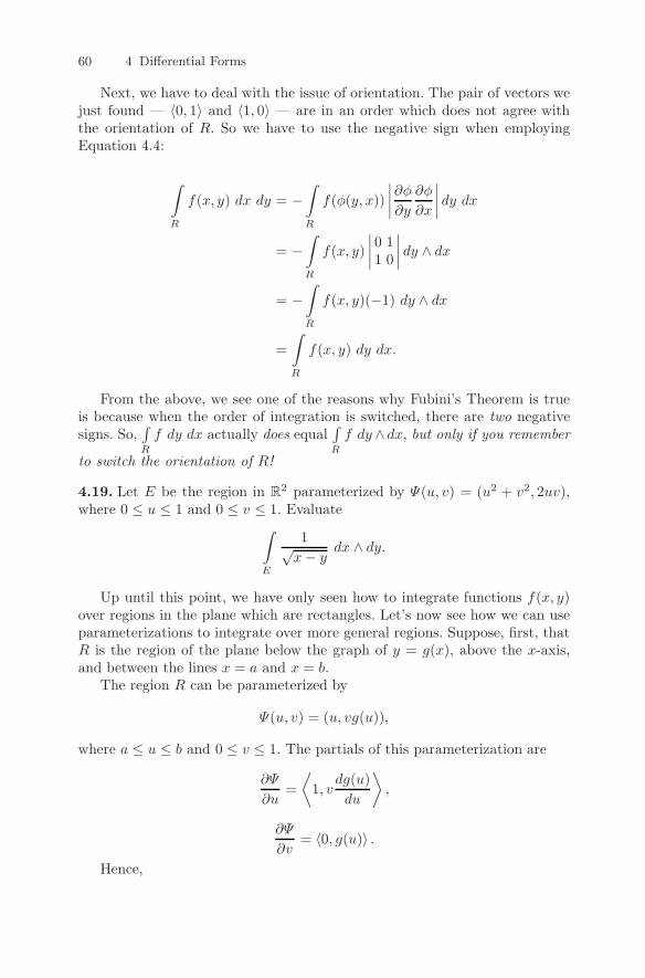
60 4 Differential Forms
Next, we have to deal with the issue of orientation. The pair of vectors wejust found — 〈0, 1〉 and 〈1, 0〉 — are in an order which does not agree withthe orientation of R. So we have to use the negative sign when employingEquation 4.4:
∫R
f(x, y) dx dy = −∫R
f(φ(y, x))
∣∣∣∣∂φ∂y ∂φ∂x∣∣∣∣ dy dx
= −∫R
f(x, y)
∣∣∣∣0 11 0
∣∣∣∣ dy ∧ dx= −
∫R
f(x, y)(−1) dy ∧ dx
=
∫R
f(x, y) dy dx.
From the above, we see one of the reasons why Fubini’s Theorem is trueis because when the order of integration is switched, there are two negativesigns. So,
∫R
f dy dx actually does equal∫R
f dy ∧dx, but only if you remember
to switch the orientation of R!
4.19. Let E be the region in R2 parameterized by Ψ(u, v) = (u2 + v2, 2uv),
where 0 ≤ u ≤ 1 and 0 ≤ v ≤ 1. Evaluate∫E
1√x− y
dx ∧ dy.
Up until this point, we have only seen how to integrate functions f(x, y)over regions in the plane which are rectangles. Let’s now see how we can useparameterizations to integrate over more general regions. Suppose, first, thatR is the region of the plane below the graph of y = g(x), above the x-axis,and between the lines x = a and x = b.
The region R can be parameterized by
Ψ(u, v) = (u, vg(u)),
where a ≤ u ≤ b and 0 ≤ v ≤ 1. The partials of this parameterization are
∂Ψ
∂u=
⟨1, v
dg(u)
du
⟩,
∂Ψ
∂v= 〈0, g(u)〉 .
Hence,
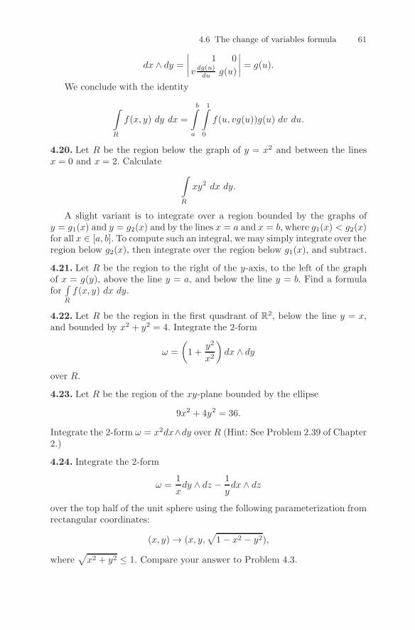
4.6 The change of variables formula 61
dx ∧ dy =
∣∣∣∣ 1 0
v dg(u)du g(u)
∣∣∣∣ = g(u).
We conclude with the identity
∫R
f(x, y) dy dx =
b∫a
1∫0
f(u, vg(u))g(u) dv du.
4.20. Let R be the region below the graph of y = x2 and between the linesx = 0 and x = 2. Calculate ∫
R
xy2 dx dy.
A slight variant is to integrate over a region bounded by the graphs ofy = g1(x) and y = g2(x) and by the lines x = a and x = b, where g1(x) < g2(x)for all x ∈ [a, b]. To compute such an integral, we may simply integrate over theregion below g2(x), then integrate over the region below g1(x), and subtract.
4.21. Let R be the region to the right of the y-axis, to the left of the graphof x = g(y), above the line y = a, and below the line y = b. Find a formulafor
∫R
f(x, y) dx dy.
4.22. Let R be the region in the first quadrant of R2, below the line y = x,and bounded by x2 + y2 = 4. Integrate the 2-form
ω =
(1 +
y2
x2
)dx ∧ dy
over R.
4.23. Let R be the region of the xy-plane bounded by the ellipse
9x2 + 4y2 = 36.
Integrate the 2-form ω = x2dx∧dy over R (Hint: See Problem 2.39 of Chapter2.)
4.24. Integrate the 2-form
ω =1
xdy ∧ dz − 1
ydx ∧ dz
over the top half of the unit sphere using the following parameterization fromrectangular coordinates:
(x, y) → (x, y,√
1− x2 − y2),
where√x2 + y2 ≤ 1. Compare your answer to Problem 4.3.
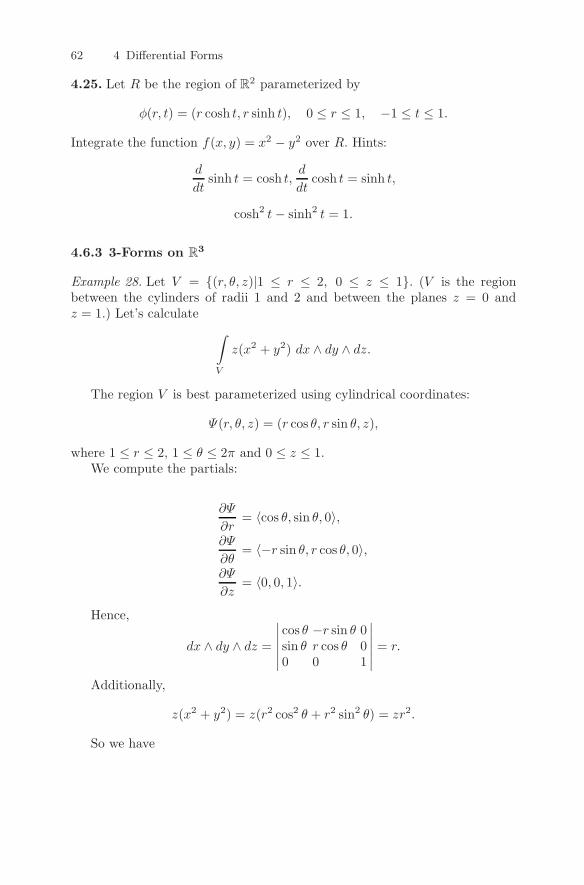
62 4 Differential Forms
4.25. Let R be the region of R2 parameterized by
φ(r, t) = (r cosh t, r sinh t), 0 ≤ r ≤ 1, −1 ≤ t ≤ 1.
Integrate the function f(x, y) = x2 − y2 over R. Hints:
d
dtsinh t = cosh t,
d
dtcosh t = sinh t,
cosh2 t− sinh2 t = 1.
4.6.3 3-Forms on R3
Example 28. Let V = (r, θ, z)|1 ≤ r ≤ 2, 0 ≤ z ≤ 1. (V is the regionbetween the cylinders of radii 1 and 2 and between the planes z = 0 andz = 1.) Let’s calculate ∫
V
z(x2 + y2) dx ∧ dy ∧ dz.
The region V is best parameterized using cylindrical coordinates:
Ψ(r, θ, z) = (r cos θ, r sin θ, z),
where 1 ≤ r ≤ 2, 1 ≤ θ ≤ 2π and 0 ≤ z ≤ 1.We compute the partials:
∂Ψ
∂r= 〈cos θ, sin θ, 0〉,
∂Ψ
∂θ= 〈−r sin θ, r cos θ, 0〉,
∂Ψ
∂z= 〈0, 0, 1〉.
Hence,
dx ∧ dy ∧ dz =∣∣∣∣∣∣cos θ −r sin θ 0sin θ r cos θ 00 0 1
∣∣∣∣∣∣ = r.
Additionally,
z(x2 + y2) = z(r2 cos2 θ + r2 sin2 θ) = zr2.
So we have
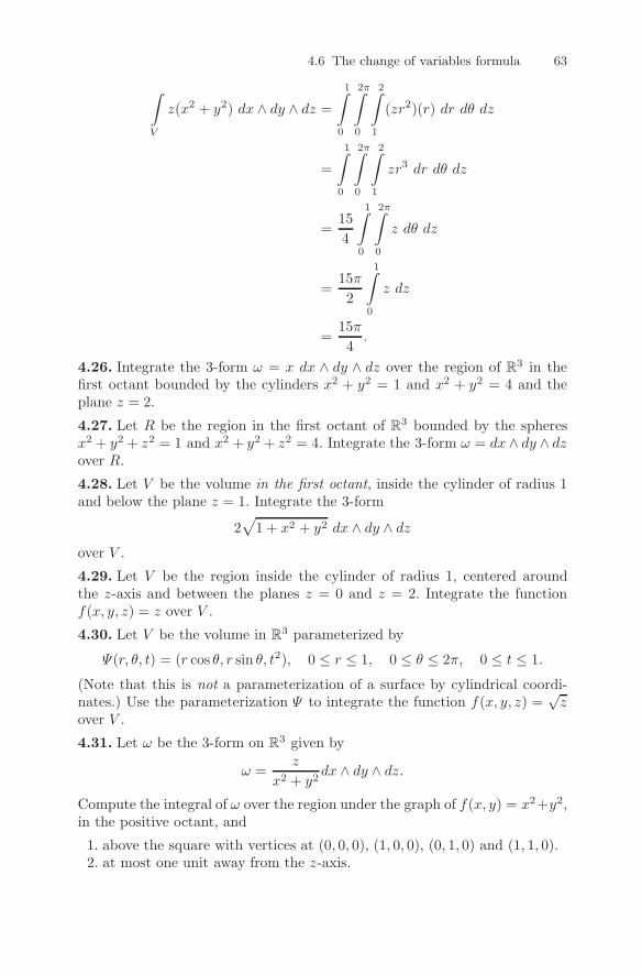
4.6 The change of variables formula 63
∫V
z(x2 + y2) dx ∧ dy ∧ dz =
1∫0
2π∫0
2∫1
(zr2)(r) dr dθ dz
=
1∫0
2π∫0
2∫1
zr3 dr dθ dz
=15
4
1∫0
2π∫0
z dθ dz
=15π
2
1∫0
z dz
=15π
4.
4.26. Integrate the 3-form ω = x dx ∧ dy ∧ dz over the region of R3 in thefirst octant bounded by the cylinders x2 + y2 = 1 and x2 + y2 = 4 and theplane z = 2.
4.27. Let R be the region in the first octant of R3 bounded by the spheresx2 + y2 + z2 = 1 and x2 + y2 + z2 = 4. Integrate the 3-form ω = dx ∧ dy ∧ dzover R.
4.28. Let V be the volume in the first octant, inside the cylinder of radius 1and below the plane z = 1. Integrate the 3-form
2√1 + x2 + y2 dx ∧ dy ∧ dz
over V .
4.29. Let V be the region inside the cylinder of radius 1, centered aroundthe z-axis and between the planes z = 0 and z = 2. Integrate the functionf(x, y, z) = z over V .
4.30. Let V be the volume in R3 parameterized by
Ψ(r, θ, t) = (r cos θ, r sin θ, t2), 0 ≤ r ≤ 1, 0 ≤ θ ≤ 2π, 0 ≤ t ≤ 1.
(Note that this is not a parameterization of a surface by cylindrical coordi-nates.) Use the parameterization Ψ to integrate the function f(x, y, z) =
√z
over V .
4.31. Let ω be the 3-form on R3 given by
ω =z
x2 + y2dx ∧ dy ∧ dz.
Compute the integral of ω over the region under the graph of f(x, y) = x2+y2,in the positive octant, and
1. above the square with vertices at (0, 0, 0), (1, 0, 0), (0, 1, 0) and (1, 1, 0).2. at most one unit away from the z-axis.
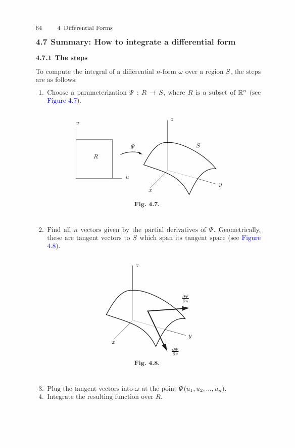
64 4 Differential Forms
4.7 Summary: How to integrate a differential form
4.7.1 The steps
To compute the integral of a differential n-form ω over a region S, the stepsare as follows:
1. Choose a parameterization Ψ : R → S, where R is a subset of Rn (seeFigure 4.7).
xy
z
Ψ
u
v
R
S
Fig. 4.7.
2. Find all n vectors given by the partial derivatives of Ψ . Geometrically,these are tangent vectors to S which span its tangent space (see Figure4.8).
xy
z
∂Ψ∂u
∂Ψ∂v
Fig. 4.8.
3. Plug the tangent vectors into ω at the point Ψ(u1, u2, ..., un).4. Integrate the resulting function over R.
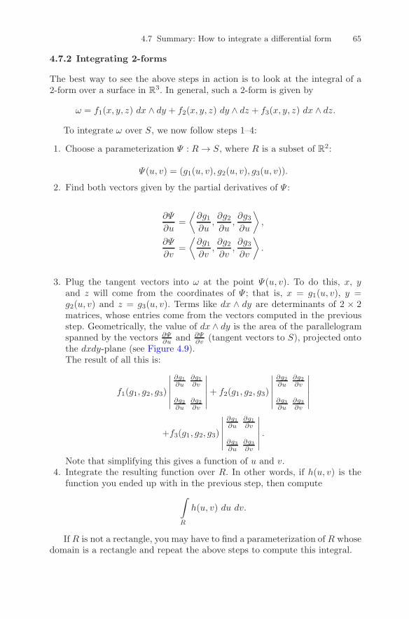
4.7 Summary: How to integrate a differential form 65
4.7.2 Integrating 2-forms
The best way to see the above steps in action is to look at the integral of a2-form over a surface in R
3. In general, such a 2-form is given by
ω = f1(x, y, z) dx ∧ dy + f2(x, y, z) dy ∧ dz + f3(x, y, z) dx ∧ dz.To integrate ω over S, we now follow steps 1–4:
1. Choose a parameterization Ψ : R → S, where R is a subset of R2:
Ψ(u, v) = (g1(u, v), g2(u, v), g3(u, v)).
2. Find both vectors given by the partial derivatives of Ψ :
∂Ψ
∂u=
⟨∂g1∂u
,∂g2∂u
,∂g3∂u
⟩,
∂Ψ
∂v=
⟨∂g1∂v
,∂g2∂v
,∂g3∂v
⟩.
3. Plug the tangent vectors into ω at the point Ψ(u, v). To do this, x, yand z will come from the coordinates of Ψ ; that is, x = g1(u, v), y =g2(u, v) and z = g3(u, v). Terms like dx ∧ dy are determinants of 2 × 2matrices, whose entries come from the vectors computed in the previousstep. Geometrically, the value of dx ∧ dy is the area of the parallelogramspanned by the vectors ∂Ψ
∂u and ∂Ψ∂v (tangent vectors to S), projected onto
the dxdy-plane (see Figure 4.9).The result of all this is:
f1(g1, g2, g3)
∣∣∣∣∣∣∂g1∂u
∂g1∂v
∂g2∂u
∂g2∂v
∣∣∣∣∣∣+ f2(g1, g2, g3)
∣∣∣∣∣∣∂g2∂u
∂g2∂v
∂g3∂u
∂g3∂v
∣∣∣∣∣∣+f3(g1, g2, g3)
∣∣∣∣∣∣∂g1∂u
∂g1∂v
∂g3∂u
∂g3∂v
∣∣∣∣∣∣ .Note that simplifying this gives a function of u and v.
4. Integrate the resulting function over R. In other words, if h(u, v) is thefunction you ended up with in the previous step, then compute∫
R
h(u, v) du dv.
If R is not a rectangle, you may have to find a parameterization of R whosedomain is a rectangle and repeat the above steps to compute this integral.
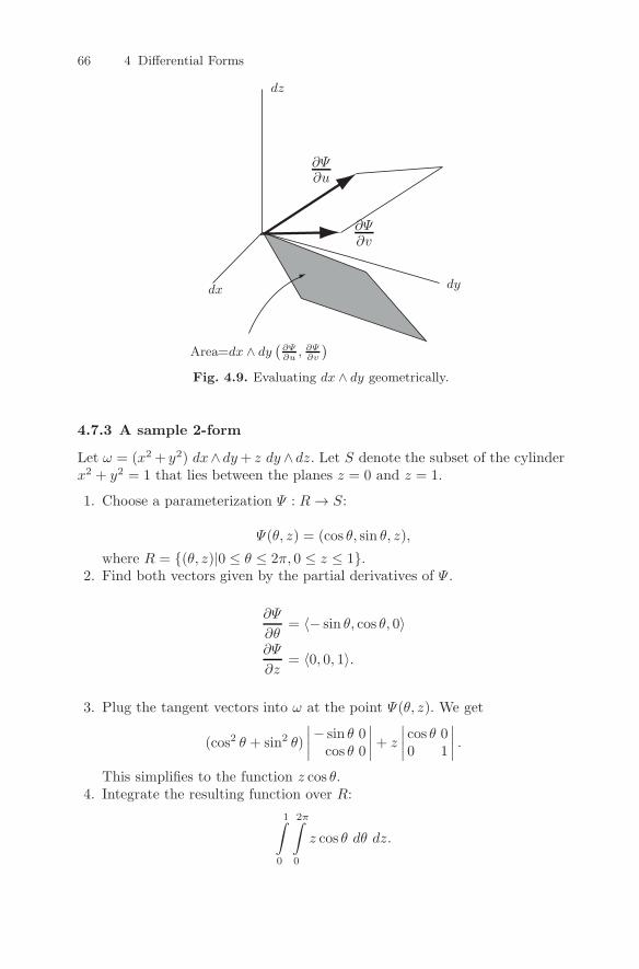
66 4 Differential Forms
dx dy
dz
∂Ψ∂u
∂Ψ∂v
Area=dx ∧ dy(∂Ψ∂u
, ∂Ψ∂v
)
Fig. 4.9. Evaluating dx ∧ dy geometrically.
4.7.3 A sample 2-form
Let ω = (x2 + y2) dx∧ dy+ z dy ∧ dz. Let S denote the subset of the cylinderx2 + y2 = 1 that lies between the planes z = 0 and z = 1.
1. Choose a parameterization Ψ : R → S:
Ψ(θ, z) = (cos θ, sin θ, z),
where R = (θ, z)|0 ≤ θ ≤ 2π, 0 ≤ z ≤ 1.2. Find both vectors given by the partial derivatives of Ψ .
∂Ψ
∂θ= 〈− sin θ, cos θ, 0〉
∂Ψ
∂z= 〈0, 0, 1〉.
3. Plug the tangent vectors into ω at the point Ψ(θ, z). We get
(cos2 θ + sin2 θ)
∣∣∣∣− sin θ 0cos θ 0
∣∣∣∣+ z
∣∣∣∣ cos θ 00 1
∣∣∣∣ .This simplifies to the function z cos θ.
4. Integrate the resulting function over R:
1∫0
2π∫0
z cos θ dθ dz.
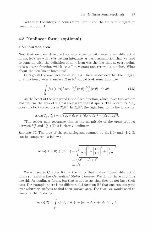
4.8 Nonlinear forms (optional) 67
Note that the integrand comes from Step 3 and the limits of integrationcome from Step 1.
4.8 Nonlinear forms (optional)
4.8.1 Surface area
Now that we have developed some proficiency with integrating differentialforms, let’s see what else we can integrate. A basic assumption that we usedto come up with the definition of an n-form was the fact that at every point,it is a linear function which “eats” n vectors and returns a number. Whatabout the non-linear functions?
Let’s go all the way back to Section 1.4. There we decided that the integralof a function f over a surface R in R
3 should look something like∫R
f(φ(r, θ))Area
[∂φ
∂r(r, θ),
∂φ
∂θ(r, θ)
]dr dθ. (4.5)
At the heart of the integrand is the Area function, which takes two vectorsand returns the area of the parallelogram that it spans. The 2-form dx ∧ dydoes this for two vectors in TpR
2. In TpR3, the right function is the following:
Area(V 1p , V
2p ) =
√(dy ∧ dz)2 + (dx ∧ dz)2 + (dx ∧ dy)2.
(The reader may recognize this as the magnitude of the cross productbetween V 1
p and V 2p .) This is clearly nonlinear!
Example 29. The area of the parallelogram spanned by 〈1, 1, 0〉 and 〈1, 2, 3〉can be computed as follows:
Area(〈1, 1, 0〉, 〈1, 2, 3〉) =√∣∣∣∣1 0
2 3
∣∣∣∣2
+
∣∣∣∣1 01 3
∣∣∣∣2
+
∣∣∣∣1 11 2
∣∣∣∣2
=√32 + 32 + 12
=√19.
We will see in Chapter 6 that the thing that makes (linear) differentialforms so useful is the Generalized Stokes Theorem. We do not have anythinglike this for nonlinear forms, but that is not to say that they do not have theiruses. For example, there is no differential 2-form on R
3 that one can integrateover arbitrary surfaces to find their surface area. For that, we would need tocompute the following:
Area(R) =
∫S
√(dy ∧ dz)2 + (dx ∧ dz)2 + (dx ∧ dy)2.
68 4 Differential Forms
For relatively simple surfaces, this integrand can be evaluated by hand.Integrals such as this play a particularly important role in certain appliedproblems. For example, if one were to dip a loop of bent wire into a soap film,the resulting surface would be the one of minimal area. Before one can evenbegin to figure out what surface this is for a given piece of wire, one must beable to know how to compute the area of an arbitrary surface, as above.
Example 30. We compute the surface area of a sphere of radius r in R3. A
parameterization is given by
Φ(θ, φ) = (r sinφ cos θ, r sinφ sin θ, r cosφ),
where 0 ≤ θ ≤ 2π and 0 ≤ φ ≤ π.Now we compute:
Area(∂Φ∂θ ,
∂Φ∂φ
)= Area (〈−r sinφ sin θ, r sinφ cos θ, 0〉, 〈r cosφ cos θ, r cosφ sin θ,−r sinφ〉)
=√
(−r2 sin2 φ cos θ)2 + (r2 sin2 φ sin θ)2 + (−r2 sinφ cosφ)2
= r2√sin4 φ+ sin2 φ cos2 φ
= r2 sinφ.
Thus, the desired area is given by
∫S
Area
(∂Φ
∂θ,∂Φ
∂φ
)dθ dφ
=
π∫0
2π∫0
r2 sinφ dθ dφ
= 4πr2.
4.32. Compute the surface area of a sphere of radius r in R3 using the pa-
rameterizationsΦ(ρ, θ) = (ρ cos θ, ρ sin θ,±
√r2 − ρ2)
for the top and bottom halves, where 0 ≤ ρ ≤ r and 0 ≤ θ ≤ 2π.
Let’s now go back to Equation 4.5. Classically, this is called a surfaceintegral. It might be a little clearer how to compute such an integral if wewrite it as follows:
∫R
f(x, y, z) dS =
∫R
f(x, y, z)√(dy ∧ dz)2 + (dx ∧ dz)2 + (dx ∧ dy)2.

4.8 Nonlinear forms (optional) 69
4.8.2 Arc length
Lengths are very similar to areas. In calculus you learn that if you have a curveC in the plane, for example, parameterized by the function φ(t) = (x(t), y(t)),where a ≤ t ≤ b, then its arc length is given by
Length(C) =
b∫a
√(dx
dt
)2
+
(dy
dt
)2
dt.
We can write this without making reference to the parameterization byemploying a nonlinear 1-form:
Length(C) =
∫C
√dx2 + dy2.
Finally, we can define what is classically called a line integral as follows:∮C
f(x, y) ds =
∫C
f(x, y)√dx2 + dy2.

5
Differentiation of Differential Forms
5.1 The derivative of a differential 1-form
The goal of this section is to figure out what we mean by the derivative of adifferential form. One way to think about a derivative is as a function whichmeasures the variation of some other function. Suppose ω is a 1-form on R
2.What do we mean by the “variation” of ω? One thing we can try is to plugin a vector field V . The result is a function from R
2 to R. We can then thinkabout how this function varies near a point p of R2. However, p can vary ina lot of ways, so we need to pick one. In Section 2.2, we learned how to takeanother vector, W , and use it to vary p. Hence, the derivative of ω, which wewill denote “dω,” is a function that acts on both V and W . In other words,it must be a 2-form!
Let’s recall how to vary a function f(x, y) in the direction of a vector Wat a point p. This was precisely the definition of the directional derivative:
∇W f(p) = ∇f(p) ·W,
where ∇f(p) is the gradient of f at p:
∇f(p) =⟨∂f
∂x(p),
∂f
∂y(p)
⟩.
Going back to the 1-form ω and the vector field V , we take the directionalderivative of the function ω(V ). Let’s do this now for a specific example.Suppose ω = y dx − x2dy, V = 〈1, 2〉, W = 〈2, 3〉 and p = (1, 1). Then ω(V )is the function y − 2x2. Now we compute:
∇Wω(V ) = ∇ω(V ) ·W = 〈−4x, 1〉 · 〈2, 3〉 = −8x+ 3.
At the point p = (1, 1) this is the number −5.What about the variation of ω(W ), in the direction of V , at the point p?
The function ω(W ) is 2y − 3x2. We now compute
DOI 10.1007/978-0-8176-830 - _5, © Springer Science+Business Media, LLC 2012, D. Bachman
4 771,A Geometric Approach to Differential Forms
72 5 Differentiation of Differential Forms
∇V ω(W ) = ∇ω(W ) · V = 〈−6x, 2〉 · 〈1, 2〉 = −6x+ 4.
At the point p = (1, 1), this is the number −2.This is a small problem. We want dω, the derivative of ω, to be a 2-form.
Hence, dω(V,W ) should equal −dω(W,V ). How can we use the variationsabove to define dω so this is true? Simple. We just define it to be the differencein these variations:
dω(V,W ) = ∇V ω(W )−∇Wω(V ). (5.1)
Hence, in the above example, dω(〈1, 2〉, 〈2, 3〉), at the point p = (1, 1), isthe number −2− (−5) = 3.
5.1. Suppose ω = xy2 dx + x3z dy − (y + z9) dz, V = 〈1, 2, 3〉 and W =〈−1, 0, 1〉.1. Compute ∇V ω(W ) and ∇Wω(V ), at the point (2, 3,−1).2. Use your answer to the previous question to compute dω(V,W ) at the
point (2, 3,−1).
There are other ways to determine what dω is rather than using Equation5.1. Recall that a 2-form acts on a pair of vectors by projecting them ontoeach coordinate plane, calculating the area they span, multiplying by someconstant, and adding. So the 2-form is completely determined by the con-stants that you multiply by after projecting. In order to figure out what theseconstants are, we are free to examine the action of the 2-form on any pair ofvectors. For example, suppose we have two vectors that lie in the xy-planeand span a parallelogram with area 1. If we run these through some 2-formand end up with the number 5, then we know that the multiplicative constantfor that 2-form, associated with the xy-plane is 5. This, in turn, tells us thatthe 2-form equals 5 dx ∧ dy + ν. To figure out what ν is, we can examine theaction of the 2-form on other pairs of vectors.
Let’s try this with a general differential 2-form on R3. Such a form always
looks like dω = a(x, y, z)dx∧dy+b(x, y, z)dy∧dz+c(x, y, z)dx∧dz. To figureout what a(x, y, z) is, for example, all we need to do is determine what dωdoes to the vectors 〈1, 0, 0〉(x,y,z) and 〈0, 1, 0〉(x,y,z). Let’s compute this usingEquation 5.1, assuming ω = f(x, y, z)dx+ g(x, y, z)dy + h(x, y, z)dz:
dω(〈1, 0, 0〉, 〈0, 1, 0〉) = ∇〈1,0,0〉ω(〈0, 1, 0〉)−∇〈0,1,0〉ω(〈1, 0, 0〉)
=
⟨∂g
∂x,∂g
∂y,∂g
∂z
⟩· 〈1, 0, 0〉 −
⟨∂f
∂x,∂f
∂y,∂f
∂z
⟩· 〈0, 1, 0〉
=∂g
∂x− ∂f
∂y.
Similarly, direct computation shows
5.2 Derivatives of n-forms 73
dω(〈0, 1, 0〉, 〈0, 0, 1〉) = ∂h
∂y− ∂g
∂z
and
dω(〈1, 0, 0〉, 〈0, 0, 1〉) = ∂h
∂x− ∂f
∂z.
Hence, we conclude that
dω =
(∂g
∂x− ∂f
∂y
)dx ∧ dy +
(∂h
∂y− ∂g
∂z
)dy ∧ dz +
(∂h
∂x− ∂f
∂z
)dx ∧ dz.
5.2. Suppose ω = f(x, y)dx + g(x, y)dy is a 1-form on R2. Show that dω =
( ∂g∂x − ∂f∂y )dx ∧ dy.
5.3. If ω = y dx−x2 dy, find dω. Verify that dω(〈1, 2〉, 〈2, 3〉) = 3 at the point(1, 1).
Technical Note: Equation 5.1 defines the value of dω as long as the vectorfields V and W are constant. If nonconstant vector fields are used, then theanswer provided by Equation 5.1 will involve partial derivatives of the com-ponents of V and W and, hence, will not be a differential form. Despite this,Equation 5.1 does lead to the correct formulas for dω, as in Exercise 5.2 above.Once such formulas are obtained, then any vector fields can be plugged in.
5.2 Derivatives of n-forms
Before jumping to the general case, let’s look at the derivative of a 2-form.A 2-form, ω, acts on a pair of vector fields, V and W , to return a function.To find some a variation of ω, we can examine how this function varies in thedirection of a third vector, U , at some point p. Hence, whatever dω turns outto be, it will be a function of the vectors U , V and W at each point p. So, wewould like to define it to be a 3-form.
Let’s start by looking at the variation of ω(V,W ) in the direction of U . Wewrite this as ∇Uω(V,W ). If we were to define this as the value of dω(U, V,W ),we would find that, in general, it would not be alternating; that is, usually∇Uω(V,W ) = −∇V ω(U,W ). To remedy this, we simply define dω to be thealternating sum of all the variations:
dω(U, V,W ) = ∇Uω(V,W )−∇V ω(U,W ) +∇Wω(U, V ).
We leave it to the reader to check that dω is alternating and multilinear(assuming U , V and W are constant vector fields).
It should not be hard for the reader to now jump to the general case.Suppose ω is an n-form and V 1, ..., V n+1 are n + 1 vector fields. Then wedefine
74 5 Differentiation of Differential Forms
dω(V 1, ..., V n+1) =
n+1∑i=1
(−1)i+1∇V i ω(V 1, ..., V i−1, V i+1, ..., V n+1).
In other words, dω, applied to n + 1 vectors, is the alternating sum of thevariations of ω applied to n of those vectors in the direction of the remainingone. Note that we can think of d as an operator which takes n-forms to (n+1)-forms.
5.4. Show that dω is alternating.
5.5. Show that d(ω + ν) = dω + dν and d(cω) = c dω, for any constant c.
5.6. Suppose ω = f(x, y, z) dx ∧ dy + g(x, y, z) dy ∧ dz + h(x, y, z) dx ∧ dz.Find dω. (Hint: Compute dω(〈1, 0, 0〉, 〈0, 1, 0〉, 〈0, 0, 1〉).) Compute d(x2y dx∧dy + y2z dy ∧ dz).
5.3 Interlude: 0-Forms
Let’s go back to Section 3.1, where we introduced coordinates for vectors. Atthat time, we noted that if C was the graph of the function y = f(x) and pwas a point of C, then the tangent line to C at p lies in TpR
2 and has theequation dy = m dx for some constant m. Of course, if p = (x0, y0), then mis just the derivative of f evaluated at x0.
Now, suppose we had looked at the graph of a function of 2-variables,z = f(x, y), instead. At some point p = (x0, y0, z0) on the graph, we could lookat the tangent plane, which lies in TpR
3. Its equation is dz = m1dx +m2dy.
Since z = f(x, y), m1 = ∂f∂x (x0, y0) and m2 = ∂f
∂y (x0, y0), we can rewrite thisas
df =∂f
∂xdx+
∂f
∂ydy.
Notice that the right-hand side of this equation is a differential 1-form. Thisis a bit strange; we applied the d operator to something and the result was a1-form. However, we know that when we apply the d operator to a differentialn-form, we get a differential (n + 1)-form. So, it must be that f(x, y) is adifferential 0-form on R
2!In retrospect, this should not be so surprising. After all, the input to a
differential n-form on Rm is a point and n vectors based at that point. So,
the input to a differential 0-form should be a point of Rm and no vectors. Inother words, a 0-form on R
m is just another word for a real-valued functionon R
m.Let’s extend some of the things we can do with forms to 0-forms. Suppose
f is a 0-form and ω is an n-form (where n may also be zero). What do wemean by f ∧ ω? Since the wedge product of an n-form and an m-form is an
5.4 Algebraic computation of derivatives 75
(n +m)-form, it must be that f ∧ ω is an n-form. It is hard to think of anyother way to define this as just the product fω.
What about integration? Remember that we integrate n-forms over subsetsof Rm that can be parameterized by a subset of Rn. So, 0-forms get integratedover things parameterized by R
0. In other words, we integrate a 0-form overa point. How do we do this? We do the simplest possible thing; define thevalue of a 0-form, f , integrated over the point p to be ±f(p). To specify anorientation, we just need to say whether or not to use the − sign. We do thisjust by writing “−p” instead of “p” when we want the integral of f over p tobe −f(p).
One word of caution here: Beware of orientations! If p ∈ Rn, then we use
the notation “−p” to denote p with the negative orientation. So if p = −3 ∈R
1, then −p is not the same as the point, 3. −p is just the point −3 with anegative orientation. So, if f(x) = x2, then
∫−pf = −f(p) = −9.
5.7. If f is the 0-form x2y3, p is the point (−1, 1), q is the point (1,−1), andr is the point (−1,−1), then compute the integral of f over the points −p,−q and −r, with the indicated orientations.
Let’s go back to our exploration of derivatives of n-forms. Suppose f(x, y) dxis a 1-form on R
2. Then we have already shown that d(f dx) = ∂f∂y dy ∧ dx.
We now compute:
df ∧ dx =
(∂f
∂xdx+
∂f
∂ydy
)∧ dx
=∂f
∂xdx ∧ dx +
∂f
∂ydy ∧ dx
=∂f
∂ydy ∧ dx
= d(f dx).
5.8. If f is a 0-form, show that d(f dx1 ∧ dx2 ∧ · · · ∧ dxn) = df ∧ dx1 ∧ dx2 ∧· · · ∧ dxn.5.9. Prove d(dω) = 0.
5.10. If ω is an n-form and µ is an m-form, then show that d(ω ∧ µ) =dω ∧ µ+ (−1)nω ∧ dµ.
5.4 Algebraic computation of derivatives
As in Section 3.7, we break with the spirit of the text to list the identities wehave acquired and work a few examples.
76 5 Differentiation of Differential Forms
Let ω be an n-form, µ an m-form, and f a 0-form. Then we have thefollowing identities:
d(dω) = 0,
d(ω + µ) = dω + dµ,
d(ω ∧ µ) = dω ∧ µ+ (−1)nω ∧ dµ,d(f dx1 ∧ dx2 ∧ · · · ∧ dxn) = df ∧ dx1 ∧ dx2 ∧ · · · ∧ dxn,
df =∂f
∂x1dx1 +
∂f
∂x2dx2 + · · ·+ ∂f
∂xndxn.
Example 31.d(xy dx− xy dy + xy2z3 dz
)= d(xy) ∧ dx− d(xy) ∧ dy + d(xy2z3) ∧ dz= (y dx+ x dy) ∧ dx− (y dx+ x dy) ∧ dy
+(y2z3 dx+ 2xyz3 dy + 3xy2z2 dz) ∧ dz=y dx ∧ dx+ x dy ∧ dx− y dx ∧ dy −x dy ∧ dy
+y2z3 dx ∧ dz + 2xyz3 dy ∧ dz +3xy2z2 dz ∧ dz
= x dy ∧ dx− y dx ∧ dy + y2z3 dx ∧ dz + 2xyz3 dy ∧ dz= −x dx ∧ dy − y dx ∧ dy + y2z3 dx ∧ dz + 2xyz3 dy ∧ dz= (−x− y) dx ∧ dy + y2z3 dx ∧ dz + 2xyz3 dy ∧ dz.
Example 32.d(x2(y + z2) dx ∧ dy + z(x3 + y) dy ∧ dz)
= d(x2(y + z2)) ∧ dx ∧ dy + d(z(x3 + y)) ∧ dy ∧ dz= 2x2z dz ∧ dx ∧ dy + 3x2z dx ∧ dy ∧ dz= 5x2z dx ∧ dy ∧ dz.
5.11. If f is the 0-form x2y3 and ω is the 1-form x2z dx + y3z2 dy (on R3),
then use the identity d(f dω) = df ∧ dω to compute d(f dω).
5.12. For each differential n-form ω, find dω.
1. x2 sin(y − z).2. sin y dx+ cosx dy.3. xy dx+ xz dy + xyz dz.4. xy2 dx+ x3z dy − (y + z9) dz.5. xz2 dx ∧ dy + xz2 dy ∧ dz.6. (x2 + y2)dy ∧ dz + (x2 − y2)dx ∧ dz.7. xy2 dy ∧ dz + x3z dx ∧ dz − (y + z9) dx ∧ dy.8. x2y3z4 dx ∧ dy ∧ dz.
5.13. Let f, g and h be functions from R3 to R. If
ω = f dy ∧ dz − g dx ∧ dz + h dx ∧ dy,then compute dω.
5.6 Application: Foliations and contact structures 77
5.5 Antiderivatives
Just as in single-variable calculus, it will be helpful to have some proficiencyin recognizing antiderivatives. Nothing substitutes for practice.
5.14. Find forms whose derivatives are
1. dx ∧ dy2. dx ∧ dy ∧ dz3. yz dx+ xz dy + xy dz4. y2z2 dx+ 2xyz2 dy + 2xy2z dz5. (y2 − 2xy) cos(xy2) dx ∧ dy.
5.15. Find two 1-forms whose derivatives are
y
xdx ∧ dy.
One should be of the form “ dx” and the other “ dy.”
5.16. Show that ω = xy2 dx is not the derivative of any 0-form. (Hint: Con-sider dω.)
5.6 Application: Foliations and contact structures
Everyone has seen tree rings and layers in sedimentary rock. These are exam-ples of foliations. Intuitively, a foliation is when some region of space has been“filled up” with lower-dimensional surfaces. A full treatment of foliations is atopic for a much larger textbook than this one. Here we will only be discussingfoliations of R3.
Let U be an open subset of R3. We say U has been foliated if there isa family φt : Rt → U of parameterizations (where for each t, the domainRt ⊂ R
2) such that every point of U is in the image of exactly one suchparameterization. In other words, the images of the parameterizations φt aresurfaces that fill up U , and no two overlap.
Suppose p is a point of U and U has been foliated as above. Then thereis a unique value of t such that p is a point in φt(Rt). The partial derivatives∂φt
∂x (p) and∂φt
∂y (p) are then two vectors that span a plane in TpR3. Let’s call
this plane Πp. In other words, if U is foliated, then at every point p of U , weget a plane Πp in TpR
3.The family Πp is an example of a plane field. In general, a plane field
is just a choice of a plane in each tangent space which varies smoothly frompoint to point in R
3. We say a plane field is integrable if it consists of thetangent planes to a foliation.
This should remind you a little of first-term calculus. If f : R1 → R1 is
a differentiable function, then at every point p on its graph, we get a line in
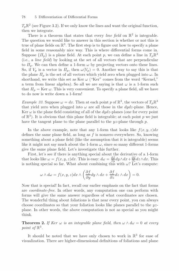
78 5 Differentiation of Differential Forms
TpR2 (see Figure 3.2). If we only know the lines and want the original function,
then we integrate.There is a theorem that states that every line field on R
2 is integrable.The question we would like to answer in this section is whether or not this istrue of plane fields on R
3. The first step is to figure out how to specify a planefield in some reasonably nice way. This is where differential forms come in.Suppose Πp is a plane field. At each point p, we can define a line in TpR
3
(i.e., a line field) by looking at the set of all vectors that are perpendicularto Πp. We can then define a 1-form ω by projecting vectors onto these lines.So, if Vp is a vector in Πp, then ω(Vp) = 0. Another way to say this is thatthe plane Πp is the set of all vectors which yield zero when plugged into ω. Inshorthand, we write this set as Ker ω (“Ker” comes from the word “Kernel,”a term from linear algebra). So all we are saying is that ω is a 1-form suchthat Πp = Ker ω. This is very convenient. To specify a plane field, all we haveto do now is write down a 1-form!
Example 33. Suppose ω = dx. Then at each point p of R3, the vectors of TpR3
that yield zero when plugged into ω are all those in the dydz-plane. Hence,Ker ω is the plane field consisting of all of the dydz-planes (one for every pointof R3). It is obvious that this plane field is integrable; at each point p we justhave the tangent plane to the plane parallel to the yz-plane through p.
In the above example, note that any 1-form that looks like f(x, y, z)dxdefines the same plane field, as long as f is nonzero everywhere. So, knowingsomething about a plane field (like the assumption that it is integrable) seemslike it might not say much about the 1-form ω, since so many different 1-formsgive the same plane field. Let’s investigate this further.
First, let’s see if there is anything special about the derivative of a 1-formthat looks like ω = f(x, y, z)dx. This is easy: dω = ∂f
∂y dy∧dx+ ∂f∂z dz∧dx. This
is nothing special so far. What about combining this with ω? Let’s compute:
ω ∧ dω = f(x, y, z)dx ∧(∂f
∂ydy ∧ dx+
∂f
∂zdz ∧ dx
)= 0.
Now that is special! In fact, recall our earlier emphasis on the fact that formsare coordinate-free. In other words, any computation one can perform withforms will give the same answer regardless of what coordinates are chosen.The wonderful thing about foliations is that near every point, you can alwayschoose coordinates so that your foliation looks like planes parallel to the yz-plane. In other words, the above computation is not as special as you mightthink.
Theorem 2. If Ker ω is an integrable plane field, then ω ∧ dω = 0 at everypoint of R3.
It should be noted that we have only chosen to work in R3 for ease of
visualization. There are higher-dimensional definitions of foliations and plane
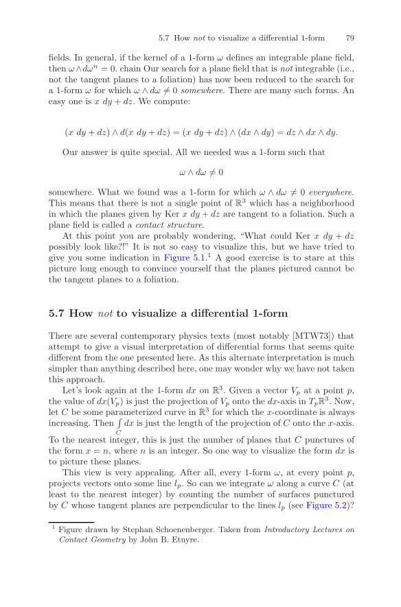
5.7 How not to visualize a differential 1-form 79
fields. In general, if the kernel of a 1-form ω defines an integrable plane field,then ω∧dωn = 0. chain Our search for a plane field that is not integrable (i.e.,not the tangent planes to a foliation) has now been reduced to the search fora 1-form ω for which ω ∧ dω = 0 somewhere. There are many such forms. Aneasy one is x dy + dz. We compute:
(x dy + dz) ∧ d(x dy + dz) = (x dy + dz) ∧ (dx ∧ dy) = dz ∧ dx ∧ dy.
Our answer is quite special. All we needed was a 1-form such that
ω ∧ dω = 0
somewhere. What we found was a 1-form for which ω ∧ dω = 0 everywhere.This means that there is not a single point of R3 which has a neighborhoodin which the planes given by Ker x dy + dz are tangent to a foliation. Such aplane field is called a contact structure.
At this point you are probably wondering, “What could Ker x dy + dzpossibly look like?!” It is not so easy to visualize this, but we have tried togive you some indication in Figure 5.1.1 A good exercise is to stare at thispicture long enough to convince yourself that the planes pictured cannot bethe tangent planes to a foliation.
5.7 How not to visualize a differential 1-form
There are several contemporary physics texts (most notably [MTW73]) thatattempt to give a visual interpretation of differential forms that seems quitedifferent from the one presented here. As this alternate interpretation is muchsimpler than anything described here, one may wonder why we have not takenthis approach.
Let’s look again at the 1-form dx on R3. Given a vector Vp at a point p,
the value of dx(Vp) is just the projection of Vp onto the dx-axis in TpR3. Now,
let C be some parameterized curve in R3 for which the x-coordinate is always
increasing. Then∫C
dx is just the length of the projection of C onto the x-axis.
To the nearest integer, this is just the number of planes that C punctures ofthe form x = n, where n is an integer. So one way to visualize the form dx isto picture these planes.
This view is very appealing. After all, every 1-form ω, at every point p,projects vectors onto some line lp. So can we integrate ω along a curve C (atleast to the nearest integer) by counting the number of surfaces puncturedby C whose tangent planes are perpendicular to the lines lp (see Figure 5.2)?
1 Figure drawn by Stephan Schoenenberger. Taken from Introductory Lectures onContact Geometry by John B. Etnyre.
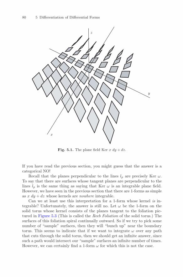
80 5 Differentiation of Differential Forms
x
y
z
Fig. 5.1. The plane field Ker x dy + dz.
If you have read the previous section, you might guess that the answer is acategorical NO!
Recall that the planes perpendicular to the lines lp are precisely Ker ω.To say that there are surfaces whose tangent planes are perpendicular to thelines lp is the same thing as saying that Ker ω is an integrable plane field.However, we have seen in the previous section that there are 1-forms as simpleas x dy + dz whose kernels are nowhere integrable.
Can we at least use this interpretation for a 1-form whose kernel is in-tegrable? Unfortunately, the answer is still no. Let ω be the 1-form on thesolid torus whose kernel consists of the planes tangent to the foliation pic-tured in Figure 5.3 (This is called the Reeb Foliation of the solid torus.) Thesurfaces of this foliation spiral continually outward. So if we try to pick somenumber of “sample” surfaces, then they will “bunch up” near the boundarytorus. This seems to indicate that if we want to integrate ω over any paththat cuts through the solid torus, then we should get an infinite answer, sincesuch a path would intersect our “sample” surfaces an infinite number of times.However, we can certainly find a 1-form ω for which this is not the case.
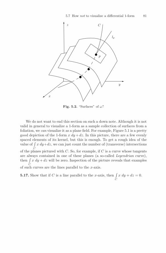
5.7 How not to visualize a differential 1-form 81
x
y
z
lp
C
p
Fig. 5.2. “Surfaces” of ω?
We do not want to end this section on such a down note. Although it is notvalid in general to visualize a 1-form as a sample collection of surfaces from afoliation, we can visualize it as a plane field. For example, Figure 5.1 is a prettygood depiction of the 1-form x dy+ dz. In this picture, there are a few evenlyspaced elements of its kernel, but this is enough. To get a rough idea of thevalue of
∫C
x dy+dz, we can just count the number of (transverse) intersections
of the planes pictured with C. So, for example, if C is a curve whose tangentsare always contained in one of these planes (a so-called Legendrian curve),then
∫C
x dy+ dz will be zero. Inspection of the picture reveals that examples
of such curves are the lines parallel to the x-axis.
5.17. Show that if C is a line parallel to the x-axis, then∫C
x dy + dz = 0.
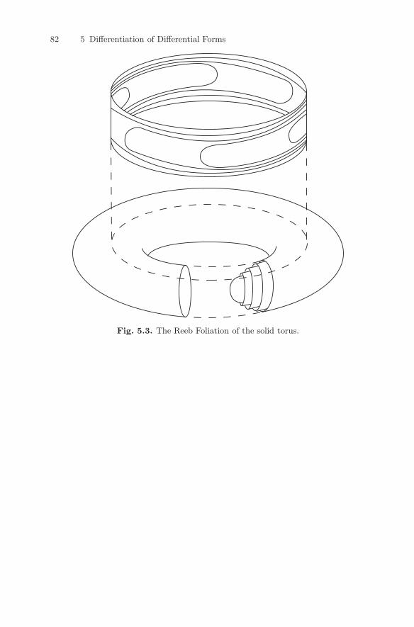
82 5 Differentiation of Differential Forms
Fig. 5.3. The Reeb Foliation of the solid torus.
6
Stokes’ Theorem
6.1 Cells and chains
Up until now, we have not been very specific as to the types of subsets of Rm
on which one integrates a differential n-form. All we have needed is a subsetthat can be parameterized by a region in R
n. To go further, we need to specifythe types of regions.
Definition 1. Let I = [0, 1]. An n-cell, σ, is the image of a differentiablemap, φ : In → R
m, with a specified orientation. We denote the same cell withopposite orientation as −σ. We define a 0-cell to be an oriented point of Rm.
Example 34. Suppose g1(x) and g2(x) are functions such that g1(x) < g2(x)for all x ∈ [a, b]. Let R denote the subset of R2 bounded by the graphs ofthe equations y = g1(x) and y = g2(x) and by the lines x = a and x = b. InExample 12, we showed that R is a 2-cell (assuming the induced orientation).
We would like to treat cells as algebraic objects which can be added andsubtracted. However, if σ is a cell, it may not at all be clear what “2σ”represents. One way to think about it is as two copies of σ, placed right ontop of each other.
Definition 2. An n-chain is a formal linear combination of n-cells.
As one would expect, we assume the following relations hold:
σ − σ = ∅,nσ +mσ = (n+m)σ,
σ + τ = τ + σ.
You may be able to guess what the integral of an n-form, ω, over an n-chainis. Suppose C =
∑niσi. Then we define
DOI 10.1007/978-0-8176-830 - _6, © Springer Science+Business Media, LLC 2012, D. Bachman
4 783,A Geometric Approach to Differential Forms
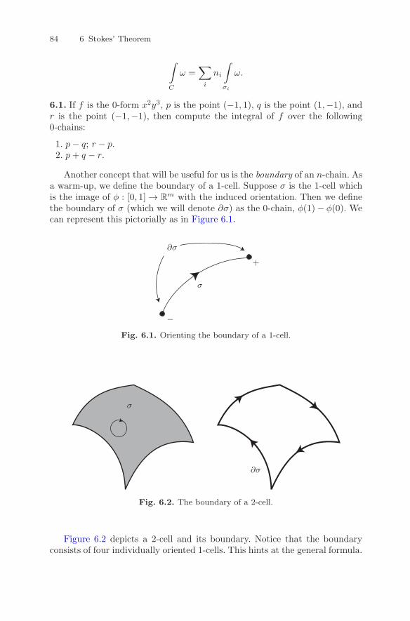
84 6 Stokes’ Theorem
∫C
ω =∑i
ni
∫σi
ω.
6.1. If f is the 0-form x2y3, p is the point (−1, 1), q is the point (1,−1), andr is the point (−1,−1), then compute the integral of f over the following0-chains:
1. p− q; r − p.2. p+ q − r.
Another concept that will be useful for us is the boundary of an n-chain. Asa warm-up, we define the boundary of a 1-cell. Suppose σ is the 1-cell whichis the image of φ : [0, 1] → R
m with the induced orientation. Then we definethe boundary of σ (which we will denote ∂σ) as the 0-chain, φ(1)− φ(0). Wecan represent this pictorially as in Figure 6.1.
σ
∂σ
+
−Fig. 6.1. Orienting the boundary of a 1-cell.
σ
∂σ
Fig. 6.2. The boundary of a 2-cell.
Figure 6.2 depicts a 2-cell and its boundary. Notice that the boundaryconsists of four individually oriented 1-cells. This hints at the general formula.
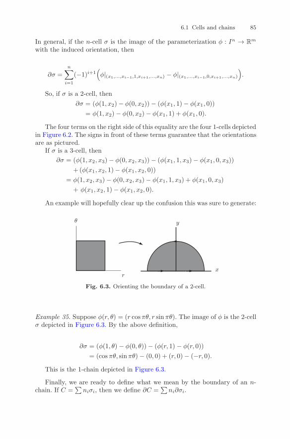
6.1 Cells and chains 85
In general, if the n-cell σ is the image of the parameterization φ : In → Rm
with the induced orientation, then
∂σ =
n∑i=1
(−1)i+1(φ|(x1,...,xi−1,1,xi+1,...,xn) − φ|(x1,...,xi−1,0,xi+1,...,xn)
).
So, if σ is a 2-cell, then
∂σ = (φ(1, x2)− φ(0, x2))− (φ(x1, 1)− φ(x1, 0))
= φ(1, x2)− φ(0, x2)− φ(x1, 1) + φ(x1, 0).
The four terms on the right side of this equality are the four 1-cells depictedin Figure 6.2. The signs in front of these terms guarantee that the orientationsare as pictured.
If σ is a 3-cell, then
∂σ = (φ(1, x2, x3)− φ(0, x2, x3))− (φ(x1, 1, x3)− φ(x1, 0, x3))
+ (φ(x1, x2, 1)− φ(x1, x2, 0))
= φ(1, x2, x3)− φ(0, x2, x3)− φ(x1, 1, x3) + φ(x1, 0, x3)
+ φ(x1, x2, 1)− φ(x1, x2, 0).
An example will hopefully clear up the confusion this was sure to generate:
x
y
r
θ
Fig. 6.3. Orienting the boundary of a 2-cell.
Example 35. Suppose φ(r, θ) = (r cosπθ, r sinπθ). The image of φ is the 2-cellσ depicted in Figure 6.3. By the above definition,
∂σ = (φ(1, θ) − φ(0, θ))− (φ(r, 1) − φ(r, 0))
= (cos πθ, sinπθ)− (0, 0) + (r, 0)− (−r, 0).This is the 1-chain depicted in Figure 6.3.
Finally, we are ready to define what we mean by the boundary of an n-chain. If C =
∑niσi, then we define ∂C =
∑ni∂σi.
86 6 Stokes’ Theorem
Example 36. Suppose
φ1(r, θ) = (r cos 2πθ, r sin 2πθ,√
1− r2),
φ2(r, θ) = (−r cos 2πθ, r sin 2πθ,−√1− r2),
σ1 = Im(φ1), and σ2 = Im(φ2). Then σ1+σ2 is a sphere in R3. One can check
that ∂(σ1 + σ2) = ∅.6.2. If σ is an n-cell, show that ∂∂σ = ∅. (At least show this if σ is a 2-celland a 3-cell. The 2-cell case can be deduced pictorially from Figures 6.1 and6.2.)
6.3. If σ is given by the parameterization
φ(r, θ) = (r cos θ, r sin θ)
for 0 ≤ r ≤ 1 and 0 ≤ θ ≤ π4 , then what is ∂σ?
6.4. If σ is given by the parameterization
φ(r, θ) = (r cos θ, r sin θ, r)
for 0 ≤ r ≤ 1 and 0 ≤ θ ≤ 2π, then what is ∂σ?
6.2 The generalized Stokes’ Theorem
In calculus, we learn that when you take a function, differentiate it, and thenintegrate the result, something special happens. In this section, we explorewhat happens when we take a form, differentiate it, and then integrate theresulting form over some chain. The general argument is quite complicated, sowe start by looking at forms of a particular type integrated over very specialregions.
Suppose ω = a dx2∧dx3 is a 2-form on R3, where a : R3 → R. Let R be the
unit cube I3 ⊂ R3. We would like to explore what happens when we integrate
dω over R. Note first that Problem 5.8 implies that dω = ∂a∂x1
dx1 ∧ dx2 ∧ dx3.Recall the steps used to define
∫R
dω:
1. Choose a lattice of points in R, pi,j,k. Since R is a cube, we can choosethis lattice to be rectangular.
2. Define V 1i,j,k = pi+1,j,k − pi,j,k. Similarly, define V 2
i,j,k and V 3i,j,k.
3. Compute dωpi,j,k(V1i,j,k, V
2i,j,k, V
2i,j,k).
4. Sum over all i, j and k.5. Take the limit as the maximal distance between adjacent lattice points
goes to zero.
6.2 The generalized Stokes’ Theorem 87
Let’s focus on Step 3 for a moment. Let t be the distance between pi+1,j,k
and pi,j,k, and assume t is small. Then ∂a∂x1
(pi,j,k) is approximately equal toa(pi+1,j,k)−a(pi,j,k)
t . This approximation gets better and better when we lett→ 0 in Step 5.
The vectors V 1i,j,k through V 3
i,j,k form a little cube. If we say the vector
V 1i,j,k is “vertical”, and the other two are horizontal, then the “height” of this
cube is t and the area of its base is dx2 ∧ dx3(V 2i,j,k, V
3i,j,k), which makes its
volume t dx2 ∧ dx3(V 2i,j,k, V
3i,j,k). Putting all this together, we find that
dωpi,j,k(V1i,j,k, V
2i,j,k, V
2i,j,k) =
∂a
∂x1dx1 ∧ dx2 ∧ dx3(V 1
i,j,k, V2i,j,k, V
2i,j,k)
≈ a(pi+1,j,k)− a(pi,j,k)
tt dx2 ∧ dx3(V 2
i,j,k, V3i,j,k)
= ω(V 2i+1,j,k, V
3i+1,j,k)− ω(V 2
i,j,k, V3i,j,k).
Let’s move on to Step 4. Here we sum over all i, j and k. Suppose forthe moment that i ranges between 1 and N . First, we fix j and k and sumover all i. The result is ω(V 2
N,j,k, V3N,j,k) − ω(V 2
1,j,k, V31,j,k). Now notice that∑
j,k
ω(V 2N,j,k, V
3N,j,k) is a Riemann Sum for the integral of ω over the “top” of
R and∑j,k
ω(V 21,j,k, V
31,j,k) is a Riemann Sum for ω over the “bottom” of R.
Finally, note that ω, evaluated on any pair of vectors which lie in the sides ofthe cube, gives zero. Hence, the integral of ω over a side of R is zero. Puttingall this together, we conclude ∫
R
dω =
∫∂R
ω. (6.1)
6.5. Prove that Equation 6.1 holds if ω = b dx1 ∧ dx3 or if ω = c dx1 ∧ dx2.Caution: Beware of signs and orientations.
6.6. Use the previous problem to conclude that if ω = a dx2 ∧ dx3 + b dx1 ∧dx3 + c dx1 ∧ dx2 is an arbitrary 2-form on R
3, then Equation 6.1 holds.
6.7. If ω is an arbitrary (n − 1)-form on Rn and R is the unit cube in R
n,then show that Equation 6.1 still holds.
In general, if C =∑niσi is an n-chain, then
∫∂C
ω =∫C
dω.
This equation is called the generalized Stokes’ Theorem. It is unquestion-ably the most crucial result of this text. In fact, everything we have done up
88 6 Stokes’ Theorem
to this point has been geared toward developing this equation and everythingthat follows will be applications of this equation. Technically, we have onlyestablished this theorem when integrating over cubes and their boundaries.We postpone the general proof to Section 7.1.
Example 37. Let ω = x dy be a 1-form on R2. Let σ be the 2-cell which is the
image of the parameterization φ(r, θ) = (r cos θ, r sin θ), where 0 ≤ r ≤ R and0 ≤ θ ≤ 2π. By the generalized Stokes’ Theorem,∫
∂σ
ω =
∫σ
dω =
∫σ
dx ∧ dy =
∫σ
dx dy = Area(σ) = πR2.
6.8. Verify directly that∫∂σ
ω = πR2.
Example 38. Let ω = x dy + y dx be a 1-form on R2 and let σ be any 2-cell.
Then∫∂σ
ω =∫σ
dω = 0.
6.9. Pick any 1-chain in R2, which bounds a 2-cell, and integrate the form
x dy + y dx over this curve.
6.10. Let ω be a differential (n− 1)-form and σ a (n+1)-cell. Use the gener-alized Stokes’ Theorem in two different ways to show
∫∂σ
dω = 0.
Example 39. Let C be the curve in R2 parameterized by φ(t) = (t2, t3), where
−1 ≤ t ≤ 1. Let f be the 0-form x2y. We use the generalized Stokes’ Theoremto calculate
∫C
df .
The curve C goes from the point (1,-1), when t = −1, to the point (1,1),when t = 1. Hence, ∂C is the 0-chain (1, 1) − (1,−1). Now we use Stokes’Theorem: ∫
C
df =
∫∂C
f =
∫(1,1)−(1,−1)
x2y = 1− (−1) = 2.
6.11. Calculate∫C
df directly.
6.12.
1. Let C be any curve in R2 which goes from the point (1, 0) to the point
(2, 2). Calculate ∫C
2xy3 dx+ 3x2y2 dy.
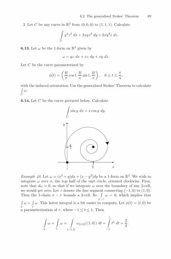
6.2 The generalized Stokes’ Theorem 89
2. Let C be any curve in R3 from (0, 0, 0) to (1, 1, 1). Calculate∫
C
y2z2 dx+ 2xyz2 dy + 2xy2z dz.
6.13. Let ω be the 1-form on R3 given by
ω = yz dx+ xz dy + xy dz.
Let C be the curve parameterized by
φ(t) =
(4t
πcos t,
4t
πsin t,
4t
π
), 0 ≤ t ≤ π
4,
with the induced orientation. Use the generalized Stokes’ Theorem to calculate∫C
ω.
6.14. Let C be the curve pictured below. Calculate∫C
sin y dx+ x cos y dy.
π2
2 x
y
Example 40. Let ω = (x2 + y)dx+ (x− y2)dy be a 1-form on R2. We wish to
integrate ω over σ, the top half of the unit circle, oriented clockwise. First,note that dω = 0, so that if we integrate ω over the boundary of any 2-cell,we would get zero. Let τ denote the line segment connecting (−1, 0) to (1, 0).Then the 1-chain σ − τ bounds a 2-cell. So
∫σ−τ
ω = 0, which implies that∫σ
ω =∫τ
ω. This latter integral is a bit easier to compute. Let φ(t) = (t, 0) be
a parameterization of τ , where −1 ≤ t ≤ 1. Then
∫σ
ω =
∫τ
ω =
∫[−1,1]
ω(t,0)(〈1, 0〉) dt =1∫
−1
t2 dt =2
3.
90 6 Stokes’ Theorem
6.15. Let ω = −y2 dx+x2 dy. Let σ be the 2-cell in R2 parameterized by the
following:φ(u, v) = (2u− v, u+ v), 1 ≤ u ≤ 2, 0 ≤ v ≤ 1.
Calculate∫∂σ
ω.
6.16. Let ω = dx− ln x dy. Let σ be the 2-cell parameterized by the following:
φ(u, v) = (uv2, u3v), 1 ≤ u ≤ 2, 1 ≤ v ≤ 2.
Calculate:∫∂σ
ω.
6.17. Let σ be the 2-cell given by the following parameterization:
φ(r, θ) = (r cos θ, r sin θ), 0 ≤ r ≤ 1, 0 ≤ θ ≤ π.
Suppose ω = x2 dx+ ey dy.
1. Calculate∫σ
dω directly.
2. Let C1 be the horizontal segment connecting (−1, 0) to (0, 0) and let C2
be the horizontal segment connecting (0, 0) to (1, 0). Calculate∫C1
ω and∫C2
ω directly.
3. Use your previous answers to determine the integral of ω over the top halfof the unit circle (oriented counterclockwise).
6.18. Let ω = (x+ y3) dx+ 3xy2 dy be a differential 1-form on R2. Let Q be
the rectangle (x, y)|0 ≤ x ≤ 3, 0 ≤ y ≤ 2.1. Compute dω.2. Use the generalized Stokes’ Theorem to compute
∫∂Q
ω.
3. Compute∫∂Q
ω directly, by integrating ω over each each edge of the bound-
ary of the rectangle and then adding in the appropriate manner.4. How does
∫R−T−L
ω compare to∫B
ω?
5. Let S be any curve in the upper half-plane (i.e., the set (x, y)|y ≥ 0)that goes from the point (3, 0) to the point (0, 0). What is
∫S
ω? Why?
6. Let S be any curve that goes from the point (3, 0) to the point (0, 0).What is
∫S
ω? Why?
6.19. Calculate ∫C
x3 dx+
(1
3x3 + xy2
)dy,
where C is the circle of radius 2, centered about the origin.
6.2 The generalized Stokes’ Theorem 91
6.20. Suppose ω = x dx + x dy is a 1-form on R2. Let C be the ellipse
x2
4 + y2
9 = 1. Determine the value of∫C
ω by integrating some 2-form over the
region bounded by the ellipse.
6.21. Let ω = −y2 dx+x2 dy. Let σ be the 2-cell in R2 parameterized by the
following:φ(r, θ) = (r cosh θ, r sinh θ),
where 0 ≤ r ≤ 1 and −1 ≤ θ ≤ 1. Calculate∫∂σ
ω.
(Recall: cosh θ =
eθ + e−θ
2, sinh θ =
eθ − e−θ
2.
)
6.22. Suppose ω is a 1-form on R2 such that dω = 0. Let C1 and C2 be the
1-cells given by the following parameterizations:
C1 : φ(t) = (t, 0), 2π ≤ t ≤ 6π
C2 : ψ(t) = (t cos t, t sin t), 2π ≤ t ≤ 6π.
Show that∫C1
ω =∫C2
ω. (Caution: Beware of orientations!)
6.23. Let S be the can-shaped surface in R3 whose side is the cylinder of
radius 1 (centered on the z-axis), and whose top and bottom are in the planesz = 1 and z = 0, respectively. Let
ω = z2 dx ∧ dyUse the generalized Stokes’ Theorem to calculate
∫S
ω (assume the standard
orientation on S).
6.24. Let V be the region between the cylinders of radii 1 and 2 (centered onthe z-axis), in the positive octant, and below the plane z = 2. Let ω be thedifferential 2-form
ω = −y3 dx ∧ dz + x3 dy ∧ dz.Calculate
∫∂V
ω.
6.25. Let ω be the following 2-form on R3:
ω = (x2 + y2)dy ∧ dz + (x2 − y2)dx ∧ dz.Let V be the region of R3 bounded by the graph of y =
√1− x2, the planes
z = 0 and z = 2, and the xz-plane (see Figure 6.4).
1. Parameterize V using cylindrical coordinates.2. Determine dω.
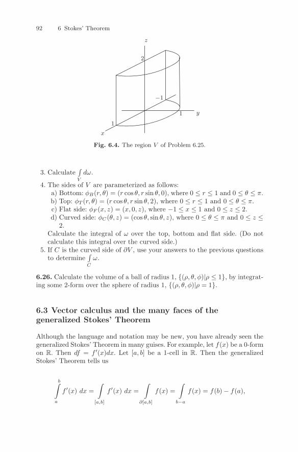
92 6 Stokes’ Theorem
x
y
z
1
1
2
−1
Fig. 6.4. The region V of Problem 6.25.
3. Calculate∫V
dω.
4. The sides of V are parameterized as follows:a) Bottom: φB(r, θ) = (r cos θ, r sin θ, 0), where 0 ≤ r ≤ 1 and 0 ≤ θ ≤ π.b) Top: φT (r, θ) = (r cos θ, r sin θ, 2), where 0 ≤ r ≤ 1 and 0 ≤ θ ≤ π.c) Flat side: φF (x, z) = (x, 0, z), where −1 ≤ x ≤ 1 and 0 ≤ z ≤ 2.d) Curved side: φC(θ, z) = (cos θ, sin θ, z), where 0 ≤ θ ≤ π and 0 ≤ z ≤
2.Calculate the integral of ω over the top, bottom and flat side. (Do notcalculate this integral over the curved side.)
5. If C is the curved side of ∂V , use your answers to the previous questionsto determine
∫C
ω.
6.26. Calculate the volume of a ball of radius 1, (ρ, θ, φ)|ρ ≤ 1, by integrat-ing some 2-form over the sphere of radius 1, (ρ, θ, φ)|ρ = 1.
6.3 Vector calculus and the many faces of thegeneralized Stokes’ Theorem
Although the language and notation may be new, you have already seen thegeneralized Stokes’ Theorem in many guises. For example, let f(x) be a 0-formon R. Then df = f ′(x)dx. Let [a, b] be a 1-cell in R. Then the generalizedStokes’ Theorem tells us
b∫a
f ′(x) dx =
∫[a,b]
f ′(x) dx =
∫∂[a,b]
f(x) =
∫b−a
f(x) = f(b)− f(a),
6.3 Vector calculus and the many faces of the generalized Stokes’ Theorem 93
which is, of course, the “Fundamental Theorem of Calculus.” If we let R besome 2-chain in R
2, then the generalized Stokes’ Theorem implies
∫∂R
P dx+Q dy =
∫R
d(P dx+Q dy) =
∫R
(∂Q
∂x− ∂P
∂y
)dx dy.
This is what we call “Green’s Theorem” in calculus. To proceed further, werestrict ourselves to R
3. In this dimension, there is a nice correspondencebetween vector fields and both 1- and 2-forms:
F = 〈Fx, Fy, Fz〉 ↔ ω1F = Fxdx+ Fydy + Fzdz
↔ ω2F = Fxdy ∧ dz − Fydx ∧ dz + Fzdx ∧ dy.
On R3 there is also a useful correspondence between 0-forms (functions) and
3-forms:f(x, y, z) ↔ ω3
f = f dx ∧ dy ∧ dz.We can use these correspondences to define various operations involving
functions and vector fields. For example, suppose f : R3 → R is a 0-form.Then df is the 1-form ∂f
∂xdx + ∂f∂y dy + ∂f
∂z dz. The vector field associated to
this 1-form is then 〈∂f∂x , ∂f∂y , ∂f∂z 〉. In calculus we call this vector field grad f ,or ∇f . In other words, ∇f is the vector field associated with the 1-form, df .This can be summarized by the equation
df = ω1∇f .
It will be useful to think of this as a diagram as well:
fgrad−−−−→ ∇f∥∥∥
f −−−−→d
df
Example 41. Suppose f = x2y3z. Then df = 2xy3z dx+3x2y2z dy+ x3y3 dz.The associated vector field, grad f , is then ∇f = 〈2xy3z, 3x2y2z, x3y3〉.
Similarly, if we start with a vector field F, form the associated 1-form ω1F,
differentiate it, and look at the corresponding vector field, then the result iscalled curl F, or ∇×F. So, ∇×F is the vector field associated with the 2-formdω1
F. This can be summarized by the equation
dω1F = ω2
∇×F.
This can also be illustrated by the following diagram:
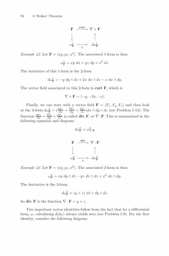
94 6 Stokes’ Theorem
Fcurl−−−−→ ∇× F
ω1F −−−−→
ddω1
F
Example 42. Let F = 〈xy, yz, x2〉. The associated 1-form is then
ω1F = xy dx + yz dy + x2 dz.
The derivative of this 1-form is the 2-form
dω1F = −y dy ∧ dz + 2x dx ∧ dz − x dx ∧ dy.
The vector field associated to this 2-form is curl F, which is
∇× F = 〈−y,−2x,−x〉.
Finally, we can start with a vector field F = 〈Fx, Fy, Fz〉 and then look
at the 3-form dω2F = (∂Fx
∂x +∂Fy
∂y + ∂Fz
∂z )dx ∧ dy ∧ dz (see Problem 5.13). The
function ∂Fx
∂x +∂Fy
∂y + ∂Fz
∂z is called div F, or ∇ ·F. This is summarized in thefollowing equation and diagram:
dω2F = ω3
∇·F
Fdiv−−−−→ ∇ · F
ω2F −−−−→
ddω2
F
Example 43. Let F = 〈xy, yz, x2〉. The associated 2-form is then
ω2F = xy dy ∧ dz − yz dx ∧ dz + x2 dx ∧ dy.
The derivative is the 3-form
dω2F = (y + z) dx ∧ dy ∧ dz.
So div F is the function ∇ · F = y + z.
Two important vector identities follow from the fact that for a differentialform, ω, calculating d(dω) always yields zero (see Problem 5.9). For the firstidentity, consider the following diagram:
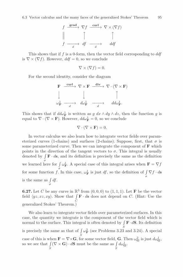
6.3 Vector calculus and the many faces of the generalized Stokes’ Theorem 95
fgrad−−−−→ ∇f curl−−−−→ ∇× (∇f)∥∥∥
f −−−−→d
df −−−−→d
ddf
This shows that if f is a 0-form, then the vector field corresponding to ddfis ∇× (∇f). However, ddf = 0, so we conclude
∇× (∇f) = 0.
For the second identity, consider the diagram
Fcurl−−−−→ ∇× F
div−−−−→ ∇ · (∇× F) ω1F −−−−→
ddω1
F −−−−→d
ddω1F.
This shows that if ddω1F is written as g dx ∧ dy ∧ dz, then the function g is
equal to ∇ · (∇× F). However, ddω1F = 0, so we conclude
∇ · (∇× F) = 0.
In vector calculus we also learn how to integrate vector fields over param-eterized curves (1-chains) and surfaces (2-chains). Suppose, first, that σ issome parameterized curve. Then we can integrate the component of F whichpoints in the direction of the tangent vectors to σ. This integral is usuallydenoted by
∫σ
F · ds, and its definition is precisely the same as the definition
we learned here for∫σ
ω1F. A special case of this integral arises when F = ∇f
for some function f . In this case, ω1F is just df , so the definition of
∫σ
∇f · dsis the same as
∫σ
df .
6.27. Let C be any curve in R3 from (0, 0, 0) to (1, 1, 1). Let F be the vector
field 〈yz, xz, xy〉. Show that∫C
F · ds does not depend on C. (Hint: Use the
generalized Stokes’ Theorem.)
We also learn to integrate vector fields over parameterized surfaces. In thiscase, the quantity we integrate is the component of the vector field which isnormal to the surface. This integral is often denoted by
∫S
F ·dS. Its definitionis precisely the same as that of
∫S
ω2F (see Problems 3.23 and 3.24). A special
case of this is when F = ∇×G, for some vector field, G. Then ω2G is just dω1
G,so we see that
∫S
(∇×G) · dS must be the same as∫S
dω1G.
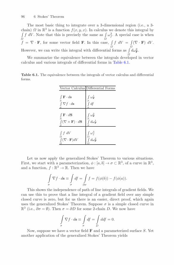
96 6 Stokes’ Theorem
The most basic thing to integrate over a 3-dimensional region (i.e., a 3-chain) Ω in R
3 is a function f(x, y, x). In calculus we denote this integral by∫Ω
f dV . Note that this is precisely the same as∫Ω
ω3f . A special case is when
f = ∇ · F, for some vector field F. In this case,∫Ω
f dV =∫Ω
(∇ · F) dV .
However, we can write this integral with differential forms as∫Ω
dω2F.
We summarize the equivalence between the integrals developed in vectorcalculus and various integrals of differential forms in Table 6.1.
Table 6.1. The equivalence between the integrals of vector calculus and differentialforms.
Vector Calculus Differential Forms
∫
σ
F · ds ∫
σ
ω1F
∫
σ
∇f · ds ∫
σ
df
∫
S
F · dS ∫
S
ω2F
∫
S
(∇× F) · dS ∫
S
dω1F
∫
Ω
f dV∫
Ω
ω3f
∫
Ω
(∇ · F)dV∫
Ω
dω2F
Let us now apply the generalized Stokes’ Theorem to various situations.First, we start with a parameterization, φ : [a, b] → σ ⊂ R
3, of a curve in R3,
and a function, f : R3 → R. Then we have∫σ
∇f · ds ≡∫σ
df =
∫∂σ
f = f(φ(b))− f(φ(a)).
This shows the independence of path of line integrals of gradient fields. Wecan use this to prove that a line integral of a gradient field over any simpleclosed curve is zero, but for us there is an easier, direct proof, which againuses the generalized Stokes’ Theorem. Suppose σ is a simple closed curve inR
3 (i.e., ∂σ = ∅). Then σ = ∂D for some 2-chain D. We now have∫σ
∇f · ds ≡∫σ
df =
∫D
ddf = 0.
Now, suppose we have a vector field F and a parameterized surface S. Yetanother application of the generalized Stokes’ Theorem yields
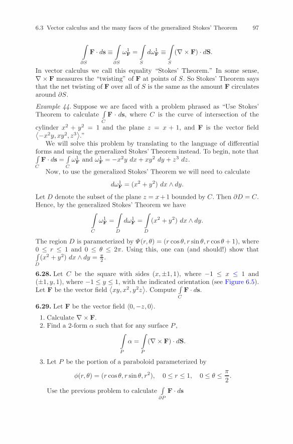
6.3 Vector calculus and the many faces of the generalized Stokes’ Theorem 97
∫∂S
F · ds ≡∫∂S
ω1F =
∫S
dω1F ≡
∫S
(∇× F) · dS.
In vector calculus we call this equality “Stokes’ Theorem.” In some sense,∇× F measures the “twisting” of F at points of S. So Stokes’ Theorem saysthat the net twisting of F over all of S is the same as the amount F circulatesaround ∂S.
Example 44. Suppose we are faced with a problem phrased as “Use Stokes’Theorem to calculate
∫C
F · ds, where C is the curve of intersection of the
cylinder x2 + y2 = 1 and the plane z = x + 1, and F is the vector field⟨−x2y, xy2, z3⟩.”We will solve this problem by translating to the language of differential
forms and using the generalized Stokes’ Theorem instead. To begin, note that∫C
F · ds = ∫C
ω1F and ω1
F = −x2y dx+ xy2 dy + z3 dz.
Now, to use the generalized Stokes’ Theorem we will need to calculate
dω1F = (x2 + y2) dx ∧ dy.
Let D denote the subset of the plane z = x+1 bounded by C. Then ∂D = C.Hence, by the generalized Stokes’ Theorem we have∫
C
ω1F =
∫D
dω1F =
∫D
(x2 + y2) dx ∧ dy.
The region D is parameterized by Ψ(r, θ) = (r cos θ, r sin θ, r cos θ+ 1), where0 ≤ r ≤ 1 and 0 ≤ θ ≤ 2π. Using this, one can (and should!) show that∫D
(x2 + y2) dx ∧ dy = π2 .
6.28. Let C be the square with sides (x,±1, 1), where −1 ≤ x ≤ 1 and(±1, y, 1), where −1 ≤ y ≤ 1, with the indicated orientation (see Figure 6.5).Let F be the vector field
⟨xy, x2, y2z
⟩. Compute
∫C
F · ds.
6.29. Let F be the vector field 〈0,−z, 0〉.1. Calculate ∇× F.2. Find a 2-form α such that for any surface P ,∫
P
α =
∫P
(∇× F) · dS.
3. Let P be the portion of a paraboloid parameterized by
φ(r, θ) = (r cos θ, r sin θ, r2), 0 ≤ r ≤ 1, 0 ≤ θ ≤ π
2.
Use the previous problem to calculate∫∂P
F · ds
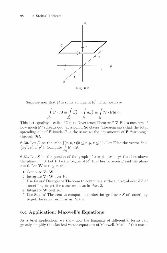
98 6 Stokes’ Theorem
x
y
z
C
Fig. 6.5.
Suppose now that Ω is some volume in R3. Then we have∫
∂Ω
F · dS ≡∫∂Ω
ω2F =
∫Ω
dω2F ≡
∫Ω
(∇ · F)dV.
This last equality is called “Gauss’ Divergence Theorem.”∇·F is a measure ofhow much F “spreads out” at a point. So Gauss’ Theorem says that the totalspreading out of F inside Ω is the same as the net amount of F “escaping”through ∂Ω.
6.30. Let Ω be the cube (x, y, z)|0 ≤ x, y, z ≤ 1. Let F be the vector field⟨xy2, y3, x2y2
⟩. Compute
∫∂Ω
F · dS.
6.31. Let S be the portion of the graph of z = 4 − x2 − y2 that lies abovethe plane z = 0. Let V be the region of R3 that lies between S and the planez = 0. Let W = 〈−y, x, z2〉.1. Compute ∇ ·W.2. Integrate ∇ ·W over V .3. Use Gauss’ Divergence Theorem to compute a surface integral over ∂V of
something to get the same result as in Part 2.4. Integrate W over ∂S.5. Use Stokes’ Theorem to compute a surface integral over S of something
to get the same result as in Part 4.
6.4 Application: Maxwell’s Equations
As a brief application, we show how the language of differential forms cangreatly simplify the classical vector equations of Maxwell. Much of this mate-
1
1
1
-1
-1
6.4 Application: Maxwell’s Equations 99
rial is taken from [MTW73], where the interested student can find many moreapplications of differential forms to physics.
Maxwell’s Equations describe the relationship between electric and mag-netic fields. Classically, both electricity and magnetism are described as a3-dimensional vector field which varies with time:
E = 〈Ex, Ey, Ez〉,B = 〈Bx, By, Bz〉,
where Ex, Ez , Ez, Bx, By and Bz are all functions of x, y, z and t.Maxwell’s Equations are then
∇ ·B = 0,
∂B
∂t+∇×E = 0,
∇ · E = 4πρ,
∂E
∂t−∇×B = −4πJ.
The quantity ρ is called the charge density and the vector J = 〈Jx, Jy, Jz〉 iscalled the current density.
We can make all of this look much simpler by making the following def-initions. First, we define a 2-form called the Faraday, which simultaneouslydescribes both the electric and magnetic fields:
F = Ex dx ∧ dt+ Ey dy ∧ dt+ Ez dz ∧ dt+Bx dy ∧ dz + By dz ∧ dx+Bz dx ∧ dy.
Next, we define the “dual” 2-form, called the Maxwell:
∗F = Ex dy ∧ dz + Ey dz ∧ dx+ Ez dx ∧ dy+Bx dt ∧ dx+By dt ∧ dy +Bz dt ∧ dz.
We also define the 4-current J and its “dual” ∗J:
J = 〈ρ, Jx, Jy, Jz〉,∗J = ρ dx ∧ dy ∧ dz,
−Jx dt ∧ dy ∧ dz,−Jy dt ∧ dz ∧ dx,−Jz dt ∧ dx ∧ dy.
Maxwell’s four vector equations now reduce to
dF = 0,
d∗F = 4π∗J
100 6 Stokes’ Theorem
6.32. Show that the equation dF = 0 implies the first two of Maxwell’s Equa-tions.
6.33. Show that the equation d∗F = 4π∗J implies the second two of Maxwell’sEquations.
The differential form version of Maxwell’s Equation has a huge advantageover the vector formulation: It is coordinate-free! A 2-form such as F is anoperator that “eats” pairs of vectors and “spits out” numbers. The way it actsis completely geometric; that is, it can be defined without any reference tothe coordinate system (t, x, y, z). This is especially poignant when one realizesthat Maxwell’s Equations are laws of nature that should not depend on a man-made construction such as coordinates.
7
Manifolds
7.1 Pull-backs
Before moving on to defining forms in more general contexts, we need tointroduce one more concept. Let’s reexamine Equation 4.3:
∫M
ω = ±∫R
ωφ(x1,...,xn)
(∂φ
∂x1(x1, ..., xn), ...,
∂φ
∂xn(x1, ..., xn)
)dx1 ∧ · · · ∧ dxn.
The form in the integrand on the right was defined so as to integrate togive the same answer as the form on the left. This is what we would like togeneralize. Suppose φ : Rn → R
m is a parameterization and ω is a k-form onRm. We define the pull-back of ω under φ to be the form on R
n which givesthe same integral over any k-cell, σ, as ω does when integrated over φ(σ).Following convention, we denote the pull-back of ω under φ as “φ∗ω.”
So how do we decide how φ∗ω acts on a k-tuple of vectors in TpRn? The
trick is to use φ to translate the vectors to a k-tuple in Tφ(p)Rm and then plug
them into ω. The matrix Dφ, whose columns are the partial derivatives of φ,is an n×m matrix. This matrix acts on vectors in TpR
n and returns vectorsin Tφ(p)R
m. So, we define (see Figure 7.1)
φ∗ω(V 1p , ..., V
kp ) = ω(Dφ(V 1
p ), ..., Dφ(Vkp )).
Example 45. Suppose ω = y dx+ z dy+ x dz is a 1-form on R3 and φ(a, b) =
(a + b, a − b, ab) is a map from R2 to R
3. Then φ∗ω will be a 1-form on R2.
To determine which one, we can examine how it acts on the vectors 〈1, 0〉(a,b)and 〈0, 1〉(a,b).
DOI 10.1007/978-0-8176-830 - _7, © Springer Science+Business Media, LLC 2012, D. Bachman
4 7101,A Geometric Approach to Differential Forms
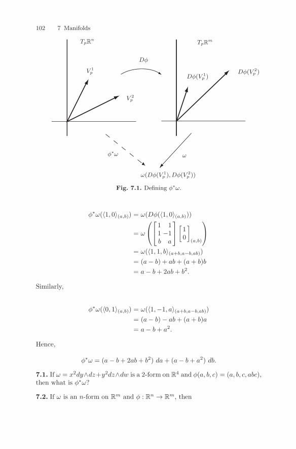
102 7 Manifolds
TpRn
TpRm
Dφ
ω
V 1p
V 2p
Dφ(V 1p )
Dφ(V 2p )
φ∗ω
ω(Dφ(V 1p ), Dφ(V 2
p ))
Fig. 7.1. Defining φ∗ω.
φ∗ω(〈1, 0〉(a,b)) = ω(Dφ(〈1, 0〉(a,b)))
= ω
1 11 −1b a
[
10
](a,b)
= ω(〈1, 1, b〉(a+b,a−b,ab))= (a− b) + ab+ (a+ b)b
= a− b+ 2ab+ b2.
Similarly,
φ∗ω(〈0, 1〉(a,b)) = ω(〈1,−1, a〉(a+b,a−b,ab))= (a− b)− ab+ (a+ b)a
= a− b+ a2.
Hence,
φ∗ω = (a− b+ 2ab+ b2) da+ (a− b+ a2) db.
7.1. If ω = x2dy∧dz+y2dz∧dw is a 2-form on R4 and φ(a, b, c) = (a, b, c, abc),
then what is φ∗ω?
7.2. If ω is an n-form on Rm and φ : Rn → R
m, then
7.2 Forms on subsets of Rn 103
φ∗ω = ωφ(x1,...,xn)
(∂φ
∂x1(x1, ..., xn), ...,
∂φ
∂xn(x1, ..., xn)
)dx1 ∧ · · · ∧ dxn.
In light of the preceding exercise, Equation 4.3 can be rewritten as∫M
ω =
∫R
φ∗ω.
7.3. If σ is a k-cell in Rn, φ : Rn → R
m, and ω is a k-form on Rm, then∫
σ
φ∗ω =
∫φ(σ)
ω.
7.4. If φ : Rn → Rm and ω is a k-form on R
m, then d(φ∗ω) = φ∗(dω).
These exercises prepare us for the proof of the generalized Stokes’ Theorem(recall that in Chapter 6 we only proved this theorem when integrating overcubes and their boundaries). Suppose σ is an n-cell in R
m, φ : In ⊂ Rn → R
m
is a parameterization of σ, and ω is an (n − 1)-form on Rm. Then we can
combine Problems 7.3, 7.4 and 6.7 to give us
∫∂σ
ω =
∫φ(∂In)
ω =
∫∂In
φ∗ω =
∫In
d(φ∗ω) =∫In
φ∗(dω) =∫
φ(In)
dω =
∫σ
dω.
7.2 Forms on subsets of Rn
The goal of this chapter is to slowly work up to defining forms in a moregeneral setting than just on R
n. One reason for this is because the generalizedStokes’ Theorem actually tells us that forms on R
n are not very interesting.For example, let’s examine how a 1-form ω on R
2, for which dω = 0 (i.e., ω isclosed), integrates over any 1-chain C such that ∂C = ∅ (i.e. C is closed). It isa basic result of topology that any such 1-chain bounds a 2-chain D. Hence,∫C
ω =∫D
dω = 0!
Fortunately, there is no reason to restrict ourselves to differential formswhich are defined on all of Rn. Instead, we can simply consider forms whichare defined on subsets, U , of Rn. For technical reasons, we will always assumesuch subsets are open. This is a technical condition which means that for eachp ∈ U , there is an ε such that
q ∈ Rn|d(p, q) < ε ⊂ U.
In this case, TUp = TRnp . Since a differential n-form is nothing more than achoice of an n-form on TRnp , for each p (with some condition about differen-tiability) it makes sense to talk about a differential form on U .
104 7 Manifolds
Example 46.
ω0 = − y
x2 + y2dx +
x
x2 + y2dy
is a differential 1-form on R2 − (0, 0).
7.5. Show that dω0 = 0.
7.6. Let C be the unit circle, oriented counterclockwise. Show that∫C
ω0 = 2π.
(Hint: Let ω′ = −y dx+ x dy. Note that on C, ω0 = ω′.)
If C is any closed 1-chain in R2− (0, 0), then the quantity 1
2π
∫C
ω0 is called
the winding number of C, since it computes the number of times C windsaround the origin.
7.7. Let x+ denote the positive x-axis in R2 − (0, 0) and let C be any closed
1-chain. Suppose Vp is a basis vector of TCp which agrees with the orientationof C at p. A positive (respectively, negative) intersection of C with x+ is onewhere Vp has a component which points “up” (respectively, “down”). Assumeall intersections of C with x+ are either positive or negative. Let P denotethe number of positive ones and N the number of negative ones. Show that12π
∫C
ω0 = P −N . (Hint: Use the generalized Stokes’ Theorem.)
We will explore the idea of winding number further in the next section.
7.3 Forms on parameterized subsets
Recall that at each point, a differential from is simply an alternating, mul-tilinear map on a tangent plane. So all we need to define a differentialform on a more general space is a well-defined tangent space. One case inwhich this happens is when we have a parameterized subset of R
m. Letφ : U ⊂ R
n → M ⊂ Rm be a (one-to-one) parameterization of M . Then
recall that TMp is defined to be the span of the partial derivatives of φ atφ−1(p) and is a n-dimensional Euclidean space, regardless of the point p.Hence, we say the dimension of M is n.
A differential k-form on M is simply an alternating, multilinear, real-valued function on TMp, for each p ∈ M , which varies differentiably with p.In other words, a differential k-form on M is a whole family of k-forms, eachone acting on TMp for different points p. It is not so easy to say preciselywhat we mean when we say the form varies in a differentiable way with p.Fortunately, we have already introduced the tools necessary to do this. Let’ssay that ω is a family of k-forms, defined on TMp, for each p ∈M . Then φ∗ωis a family of k-forms, defined on TRnφ−1(p) for each p ∈M . We say that ω isa differentiable k-form on M if φ∗ω is a differentiable family on U .
7.4 Forms on quotients of Rn (optional) 105
This definition illustrates an important technique which is often used whendealing with differential forms on manifolds. Rather than working in M di-rectly, we use the map φ∗ to translate problems about forms on M into prob-lems about forms on U . These are nice because we already know how to workwith forms which are defined on open subsets of Rn. We will have much moreto say about this later.
Example 47. The infinitely long cylinder L of radius 1, centered along the z-
axis, is given by the parameterization, φ(a, b) =(
a√a2+b2
, b√a2+b2
, ln√a2 + b2
),
whose domain is R2− (0, 0). We can use φ∗ to solve any problem about formson L by translating it back to a problem about forms on U .
7.8. Consider the 1-form τ ′ = −y dx + x dy on R3. In particular, this form
acts on vectors in TLp, where L is the cylinder of the previous example andp is any point in L. Let τ be the restriction of τ ′ to vectors in TLp. So, τ is a1-form on L. Compute φ∗τ . What does this tell you that τ measures?
If ω is a k-form on M , then what do we mean by dω? Whatever thedefinition, we clearly want dφ∗ω = φ∗dω. So why do we not use this to definedω? After all, we know what dφ∗ω is, since φ∗ω is a form on R
n. Recall thatDφp is a map from TRnp to TRmp . However, if we restrict the range to TMp,then Dφp is one-to-one, so it makes sense to refer to Dφ−1
p . We now define
dω(V 1p , ..., V
k+1p ) = dφ∗ω(Dφ−1
p (V 1p ), ..., Dφ
−1p (V k+1
p )).
7.9. If τ ′ and τ are the 1-forms on R3 and L, respectively, defined in the
previous problem, compute dτ ′ and dτ .
7.4 Forms on quotients of Rn (optional)
This section requires some knowledge of topology and algebra. It is not essen-tial for the flow of the text.
While we are on the subject of differential forms on subsets of Rn, thereis a very common construction of a topological space for which it is veryeasy to define what we mean by a differential form. Let’s look again at thecylinder L of the previous section. One way to construct L is to start withthe plane R
2 and “roll it up.” More technically, we can consider the mapµ(θ, z) = (cos θ, sin θ, z). In general, this is a many-to-one map, so it is nota parameterization in the strict sense. To remedy this, one might try andrestrict the domain of µ to (θ, z) ∈ R
2|0 ≤ θ < 2π; however, this set is notopen.
Note that for each point (θ, z) ∈ R2, Dµ is a one-to-one map from TR2
(θ,z)
to TLµ(θ,z). This is all we need in order for µ∗τ to make sense, where τ is theform on L defined in the previous section.
106 7 Manifolds
7.10. Show that µ∗τ = dθ.
In this case, we say that µ is a covering map, R2 is a cover of L, and dθ isthe lift of τ to R
2.
7.11. Suppose ω0 is the 1-form on R2 which we used to define the winding
number (see Section 7.2). Let µ(r, θ) = (r cos θ, r sin θ). Let U = (r, θ)|r > 0.Then µ : U → R2 − (0, 0) is a covering map. Hence, there is a one-to-onecorrespondence between a quotient of U and R
2 − (0, 0). Compute the lift ofω0 to U .
Let’s go back to the cylinder L. Another way to look at things is to ask:How can we recover L from the θz-plane? The answer is to view L as a quotientspace. Let’s put an equivalence relation R on the points of R
2: (θ1, z1) ∼(θ2, z2) if and only if z1 = z2 and θ1 − θ2 = 2nπ, for some n ∈ Z. We willdenote the quotient of R2 under this relation as R2/R. µ now induces a one-to-one map µ from R
2/R onto L. Hence, these two spaces are homeomorphic.
Let’s suppose now that we have a form on U , an open subset of Rn, andwe would like to know when it descends to a form on a quotient of U . Clearly,if we begin with the lift of a form, then it will descend. Let’s try and see why.In general, if µ : U ⊂ R
n → M ⊂ Rm is a many-to-one map, differentiable
at each point of U , then the sets µ−1(p) partition U . Hence, we can formthe quotient space U/µ−1 under this partition. For each x ∈ µ−1(p), Dµx is aone-to-one map from TUx to TMp and, hence, Dµ
−1x is welldefined. If x and y
are both in µ−1(p), then Dµ−1y Dµx is a one-to-one map from TUx to TUy.
We will denote this map as Dµxy. We say a k-form ω on Rn descends to a
k-form on U/µ−1 if and only if ω(V 1x , ..., V
kx ) = ω(Dµxy(V
1x ), ..., Dµxy(V
1x )),
for all x, y ∈ U such that µ(x) = µ(y).
7.12. If τ is a differential k-form onM , then µ∗τ (the lift of τ) is a differentialk-form on U which descends to a differential k-form on U/µ−1.
Now, suppose that we have a k-form ω on U which descends to a k-formon U/µ−1, where µ : U ⊂ R
n →M ⊂ Rm is a covering map. How can we get a
k-form on M? As we have already remarked, µ : U/µ−1 → M is a one-to-onemap. Hence, we can use it to push forward the form ω. In other words, we candefine a k-form on M as follows: Given k vectors in TMp, we first choose apoint x ∈ µ−1(p). We then define
µ∗ω(V 1p , ..., V
kp ) = ω(Dµ−1
x (V 1p ), ..., Dµ
−1x (V kp )).
It follows from the fact that ω descends to a form on U/µ−1 that it doesnot matter which point x we choose in µ−1(p). Note that although µ is notone-to-one, Dµx is, so Dµ−1
x makes sense.If we begin with a form on U , there is a slightly more general construction
of a form on a quotient of U , which does not require the use of a covering
7.4 Forms on quotients of Rn (optional) 107
map. Let Γ be a group of transformations of U . We say Γ acts discretely iffor each p ∈ U , there exists an ε > 0 such that Nε(p) does not contain γ(p),for any nonidentity element γ ∈ Γ . If Γ acts discretely, then we can form thequotient of U by Γ , denoted U/Γ , as follows: p ∼ q if there exists γ ∈ Γ suchthat γ(p) = q. (The fact that Γ acts discretely is what guarantees a “nice”topology on U/Γ .)
Now, suppose ω is a k-form on U . We say ω descends to a k-form ω onU/Γ if and only if ω(V 1
p , ..., Vkp ) = ω(Dγ(V 1
p ), ..., Dγ(Vkp )), for all γ ∈ Γ .
Now that we have decided what a form on a quotient of U is, we still haveto define n-chains and what we mean by integration of n-forms over n-chains.We say an n-chain C ⊂ U descends to an n-chain C ⊂ U/Γ if γ(C) = C, forall γ ∈ Γ . The n-chains of U/Γ are simply those which are descendants ofn-chains in U .
Integration is a little more subtle. For this we need the concept of a funda-mental domain for Γ . This is nothing more than a closed subset of U , whoseinterior does not contain two equivalent points. Furthermore, for each equiva-lence class, there is at least one representative in a fundamental domain. Hereis one way to construct a fundamental domain: First, choose a point p ∈ U .Now, let D = q ∈ U |d(p, q) ≤ d(γ(p), q), for all γ ∈ Γ.
Now, let C be an n-chain on U which descends to an n-chain C on U/Γand let ω be an n-form that descends to an n-form ω. Let D be a fundamentaldomain for Γ in U . Then we define∫
C
ω ≡∫
C∩D
ω.
Technical Note: In general, this definition is invariant of which pointwas chosen in the construction of the fundamental domain D. However, aVERY unlucky choice will result in C ∩D ⊂ ∂D, which could give a differentanswer for the above integral. Fortunately, it can be shown that the set of such“unlucky” points has measure zero; that is, if we were to choose the point atrandom, then the odds of picking an “unlucky” point are 0%. Very unluckyindeed!
Example 48. Suppose Γ is the group of transformations of the plane generatedby (x, y) → (x+1, y) and (x, y) → (x, y+1). The space R2/Γ is often denotedT 2 and referred to as a torus. Topologists often visualize the torus as thesurface of a donut. A fundamental domain for Γ is the unit square in R
2. The1-form dx on R
2 descends to a 1-form on T 2. Integration of this form over aclosed 1-chain C ⊂ T 2 counts the number of times C wraps around the “hole”of the donut.
108 7 Manifolds
7.5 Defining manifolds
As we have already remarked, a differential n-form on Rm is just an n-form
on TpRm, for each point p ∈ R
m, along with some condition about how theform varies in a differentiable way as p varies. All we need to define a formon a space other than R
m is some notion of a tangent space at every point.We call such a space a manifold. In addition, we insist that at each point of amanifold, the tangent space has the same dimension, n, which we then say isthe dimension of the manifold.
How do we guarantee that a given subset of Rm is a manifold? Recall
that we defined the tangent space to be the span of some partial derivativesof a parameterization. However, insisting that the whole manifold is capableof being parameterized is very restrictive. Instead, we only insist that everypoint of a manifold lies in a subset that can be parameterized. Hence, if Mis an n-manifold in R
m, then there is a set of open subsets, Ui ⊂ Rn, and
a set of differentiable maps, φi : Ui → M, such that φi(Ui) is a cover ofM (i.e., for each point p ∈ M there is an i, and a point q ∈ Ui, such thatφi(q) = p).
Example 49. S1, the unit circle in R2, is a 1-manifold. Let Ui = (−1, 1) fori = 1, 2, 3, 4, φ1(t) = (t,
√1− t2), φ2(t) = (t,−√
1− t2), φ3(t) = (√1− t2, t)
and φ4(t) = (−√1− t2, t). Then φi(Ui) is certainly a cover of S1 with the
desired properties.
7.13. Show that S2, the unit sphere in R3, is a 2-manifold.
7.6 Differential forms on manifolds
Basically, the definition of a differential n-form on an m-manifold is the sameas the definition of an n-form on a subset of Rm which was given by a singleparameterization. First and foremost, it is just an n-form on TpM , for eachp ∈M .
Let’s say M is an m-manifold. Then we know there is a set of open setsUi ⊂ R
m and a set of differentiable maps φi : Ui →M such that φi(Ui)covers M . Now, let’s say that ω is a family of n-forms, defined on TpM foreach p ∈M . Then we say that the family ω is a differentiable n-form on M ifφ∗i ω is a differentiable n-form on Ui, for each i.
Example 50. In the previous section, we saw how S1, the unit circle in R2, is
a 1-manifold. If (x, y) is a point of S1, then TS1(x,y) is given by the equation
dy = −xy dx in TR2
(x,y) as long as y = 0. If y = 0, then TS1(x,y) is given by
dx = 0. We define a 1-form on S1, ω = −y dx+x dy. (Actually, ω is a 1-formon all of R2. To get a 1-form on just S1, we restrict the domain of ω to thetangent lines to S1.) To check that this is really a differential form, we mustcompute all pull-backs:
7.6 Differential forms on manifolds 109
φ∗1ω =−1√1− t2
dt, φ∗2ω =1√
1− t2dt,
φ∗3ω =1√
1− t2dt, φ∗4ω =
−1√1− t2
dt.
Since all of these are differentiable on Ui = (−1, 1), we can say that ω is adifferential form on S1.
We now move on to integration of n-chains on manifolds. The definitionof an n-chain is no different than before; it is just a formal linear combinationof n-cells in M . Let’s suppose that C is an n-chain in M and ω is an n-form.Then how do we define
∫C
ω? If C lies entirely in φi(Ui), for some i, then we
could define the value of this integral to be the value of∫
φ−1i (C)
φ∗i ω. However,
it may be that part of C lies in both φi(Ui) and φj(Uj). If we define∫C
ω to
be the sum of the two integrals we get when we pull-back ω under φi and φj ,then we end up “double counting” the integral of ω on C ∩ φi(Ui) ∩ φj(Uj).Somehow, as we move from φi(Ui) into φj(Uj), we want the effect of the pull-back of ω under φi to “fade out” and the effect of the pull-back under φj to“fade in.” This is accomplished by a partition of unity.
The technical definition of a partition of unity subordinate to the coverφi(Ui) is a set of differentiable functions fi :M → [0, 1] such that fi(p) = 0if p /∈ φi(Ui) and
∑i
fi(p) = 1 for all p ∈M . We refer the reader to any book
on differential topology for a proof of the existence of partitions of unity.We are now ready to give the full definition of the integral of an n-form
on an n-chain in an m-manifold:∫C
ω ≡∑i
∫φ−1i (C)
φ∗i (fiω).
We illustrate this with a simple example.
Example 51. Let M be the manifold which is the interval (1, 10) ⊂ R. LetUi = (i, i+ 2) for i = 1, ..., 8. Let φi : Ui → M be the identity map. Let fibe a partition of unity, subordinate to the cover, φi(Ui). Let ω be a 1-formon M . Finally, let C be the 1-chain which consists of the single 1-cell [2, 8].Then we have
∫C
ω ≡8∑i=1
∫φ−1i (C)
φ∗i (fiω) =8∑i=1
∫C
fiω =
∫C
8∑i=1
(fiω) =
∫C
(8∑i=1
fi
)ω =
∫C
ω,
as one would expect!
110 7 Manifolds
Example 52. Let S1, Ui, φi and ω be defined as in Examples 49 and 50. Apartition of unity subordinate to the cover φi(Ui) is as follows:
f1(x, y) =
y2, y ≥ 00, y < 0
, f2(x, y) =
0, y > 0y2, y ≤ 0
,
f3(x, y) =
x2, x ≥ 00, x < 0
, f4(x, y) =
0, x > 0x2, x ≤ 0
.
(Check this!) Let µ : [0, π] → S1 be defined by µ(θ) = (cos θ, sin θ). Then theimage of µ is a 1-cell, σ, in S1. Let’s integrate ω over σ:
∫σ
ω ≡4∑i=1
∫φ−1i (σ)
φ∗i (fiω)
=
∫−(−1,1)
−√1− t2 dt+ 0 +
∫[0,1)
√1− t2 dt+
∫−[0,1)
−√1− t2 dt
=
1∫−1
√1− t2 dt+ 2
1∫0
√1− t2 dt
= π.
CAUTION: Beware of orientations!
7.7 Application: DeRham Cohomology
One of the predominant uses of differential forms is to give global informationabout manifolds. Consider the space R2− (0, 0), as in Example 46. Near everypoint of this space we can find an open set which is identical to an open setaround a point of R2. This means that all of the local information in R
2−(0, 0)is the same as the local information in R
2. The fact that the origin is missingis a global property.
For the purposes of detecting global properties, certain forms are interest-ing and certain forms are completely uninteresting. We will spend some timediscussing both. The interesting forms are the ones whose derivative is zero.Such forms are said to be closed. An example of a closed 1-form was ω0, fromExample 46. For now, let’s just focus on closed 1-forms so that you can keepthis example in mind.
Let’s look at what happens when we integrate a closed 1-form ω0 over a1-chain C such that ∂C = 0 (i.e., C is a closed 1-chain). If C bounds a diskD, then Stokes’ Theorem states
7.7 Application: DeRham Cohomology 111∫C
ω0 =
∫D
dω0 =
∫D
0 = 0.
In a sufficiently small region of every manifold, every closed 1-chain bounds adisk. So integrating closed 1-forms on “small” 1-chains gives us no information.In other words, closed 1-forms give no local information.
Suppose now that we have a closed 1-form ω0 and a closed 1-chain C suchthat
∫C
ω0 = 0. Then we know C does not bound a disk. The fact that there
exists such a 1-chain is global information. This is why we say that the closedforms are the ones that are interesting, from the point of view of detectingonly global information.
Now, let’s suppose that we have a 1-form ω1 that is the derivative of a0-form f (i.e., ω1 = df). We say such a form is exact. Again, let C be a closed1-chain. Let’s pick two points – p and q – on C. Then C = C1 + C2, whereC1 goes from p to q and C2 goes from q back to p. Now, let’s do a quickcomputation:
∫C
ω1 =
∫C1+C2
ω1
=
∫C1
ω1 +
∫C2
ω1
=
∫C1
df +
∫C2
df
=
∫p−q
f +
∫q−p
f
= 0.
So integrating an exact form over a closed 1-chain always gives zero. Thisis why we say the exact forms are completely uninteresting. Unfortunately, inProblem 5.9 we learned that every exact form is also closed. This is a problem,since this would say that all of the completely uninteresting forms are alsointeresting! To remedy, this we define an equivalence relation.
We pause here for a moment to explain what this means. An equivalencerelation is just a way of taking one set and creating a new set by declaringcertain objects in the original set to be “the same.” This is the idea behindtelling time. To construct the clock numbers, start with the integers and de-clare two to be “the same” if they differ by a multiple of 12. So, 10 + 3 = 13,but 13 is the same as 1 — so if it’s now 10 o’clock, then in three hours it willone o’clock.
We play the same trick for differential forms. We will restrict ourselvesto the closed forms, but we will consider two of them to be “the same” if
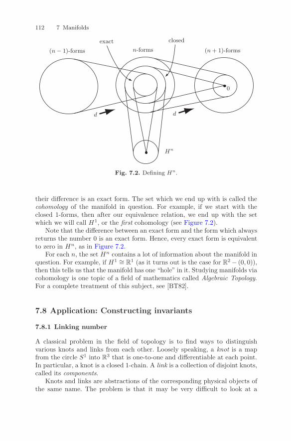
112 7 Manifolds
Hn
dd
(n− 1)-forms n-forms (n+ 1)-forms
closedexact
0
Fig. 7.2. Defining Hn.
their difference is an exact form. The set which we end up with is called thecohomology of the manifold in question. For example, if we start with theclosed 1-forms, then after our equivalence relation, we end up with the setwhich we will call H1, or the first cohomology (see Figure 7.2).
Note that the difference between an exact form and the form which alwaysreturns the number 0 is an exact form. Hence, every exact form is equivalentto zero in Hn, as in Figure 7.2.
For each n, the set Hn contains a lot of information about the manifold inquestion. For example, if H1 ∼= R
1 (as it turns out is the case for R2 − (0, 0)),then this tells us that the manifold has one “hole” in it. Studying manifolds viacohomology is one topic of a field of mathematics called Algebraic Topology.For a complete treatment of this subject, see [BT82].
7.8 Application: Constructing invariants
7.8.1 Linking number
A classical problem in the field of topology is to find ways to distinguishvarious knots and links from each other. Loosely speaking, a knot is a mapfrom the circle S1 into R
3 that is one-to-one and differentiable at each point.In particular, a knot is a closed 1-chain. A link is a collection of disjoint knots,called its components.
Knots and links are abstractions of the corresponding physical objects ofthe same name. The problem is that it may be very difficult to look at a
7.8 Application: Constructing invariants 113
physical link and tell if the individual components can be separated withoutcutting one of the links. In this section we will see that integrating a differentialform in an appropriate way over a link can yield a measure of just how “linked”its components are.
To begin, recall the 1-form ω0 from Section 7.2 whose integral yields thewinding number
ω0 = − y
x2 + y2dx+
x
x2 + y2dy.
7.14. Let A(x, y) = tan−1 yx . Thinking of A as a 0-form, show that dA = ω0.
7.15. The function A(x, y) from the previous problem gives the angle θ of thepoint (x, y) in polar coordinates; that is, θ = A(x, y). Another way to viewthis is to think of A as a function from R
2− (0, 0) to S1, the circle.1 The formdθ is the one on S1 that gives the length of any tangent vector to it. Such aform is called a length form. Show that dA = A∗dθ.
Combining the previous two problems gives the result A∗dθ = ω0; thatis, the winding number is computed by integrating the pull-back of the lengthform on S1. This interpretation is precisely what we generalize to define thelinking number of a two-component link.
Now, suppose α : S1 → R2 − (0, 0) is a parameterization of a loop (i.e.,
closed 1-chain). One way to think about integrating ω0 over the image of α isto pull-back the 1-form ω0 by the map α∗ and integrate the resulting 1-formover the domain of α. Since ω0 = A∗dθ, this is equivalent to integrating theform (A α)∗dθ over the domain of α. Here A α is the map from S1 to S1
given by the composition of A and α. So for each point t in the domain of α,A α(t) gives the angle θ of the point α(t) in R
2. Finally, we conclude thatthe winding number of α is given by
1
2π
∫α
ω0 =1
2π
∫α
A∗dθ =1
2π
∫S1
(A α)∗dθ.
To make the transition to parameterized curves in three dimensions, firstnote that the form ω0 can itself be thought of as a 1-form on the complementof the z-axis in R
3. As such, its integral over a knot (i.e., a closed, connected1-chain) tells us how much the knot winds around, or “links,” the z-axis.Just as the winding number in the plane can be computed by counting theintersections with the positive x-axis in the appropriate way (see Problem 7.7),the winding number around the z-axis in R
3 can be computed by countingthe intersections with the half of the xz-plane where x > 0.
The linking number of a two-component link is precisely the analogousmeasure that you get when you treat one of the components as the z-axisand the other as the 1-chain over which we integrate. Given any knot K in
1 Here we are thinking of the circle S1 as the interval [0, 2π], where 0 has beenidentified with 2π
114 7 Manifolds
R3, there is a function A : R3 − K → S1. (The existence of such a function
is, unfortunately, beyond the scope of this book.) If we think of A as a 0-form, then we can differentiate it to get a 1-form on R
3 −K. This 1-form isprecisely what we can integrate over a second knot to measure how many timesit “links” with K. Interestingly, there is also a point p ∈ S1 such that A−1(p)is a surface whose boundary is K. Just as before, the linking number can alsobe computed just by appropriately counting the number of intersections withthis surface.
There is a second way to view the linking number that may be of morehistorical importance than practical. Suppose α : S1 → R
3 and β : S1 → R3
are parameterizations of the two components of some link. So, for each valueof s and t, α(s) is a point on the first component and β(t) is a point on thesecond. The vector α(s)−β(t) then connects one of these points to the other.We can turn this into a unit vector in R
3 by dividing it by its magnitude.This defines a map
φ(s, t) =α(s) − β(t)
|α(s) − β(t)| .
Note that the domain of φ consists of pairs of points – s and t – from twodifferent circles. This is more commonly denoted S1 × S1, or even T 2. Therange of φ is a set of unit vectors in R
3. We can thus think of it as points onthe unit sphere, commonly denoted S2. Thus, φ is a map from T 2 to S2. Thisis completely analogous to the function A α that we encountered earlier inthe section.
Let µ denote the area form on S2; that is, µ is the 2-form that gives thearea of the parallelogram spanned by the pair tangent vectors to S2 that youplug into it. This is analogous to the 1-form dθ which computed the length oftangent vectors to the circle S1.
The linking number of α and β is given by
1
4π
∫T 2
φ∗µ.
In other words, the linking number is computed by integrating the pull-back ofthe area form on S2.
7.16. Show that∫T 2
φ∗µ =
∫∫ ∣∣∣∣∂φ∂s × ∂φ
∂t
∣∣∣∣ ds dt=
∫∫ (dα
ds× dβ
dt
)· α(s) − β(t)
|α(s)− β(t)|3 ds dt
Historical note: The linking number was first defined by Gauss when hewas studying the orbits of celestial bodies. Note that the orbits of two suchobjects forms a link in space. Later it was shown that linking number can be
7.8 Application: Constructing invariants 115
used to compute the current that is induced in one loop of wire when a givencurrent flows through another.
7.8.2 The Hopf Invariant
The mathematician Heinz Hopf was interested in studying functions from S3,the unit sphere in R
4, to S2, the unit sphere in R3. In particular, he was
looking for a quantity that did not change under small alterations of sucha map. Such a quantity is called a homotopy invariant. Finding maps withdifferent homotopy invariants then says they are fundamentally different; youcan’t get from one to another by small alterations.
Hopf’s invariant illustrates many of the tools we have developed thus far.It is not difficult for us to construct, as long as we are willing to assume oneunsurprising result from algebraic topology: The first and second cohomologyof S3 is trivial. One might expect this, as cohomology is designed to detectnontrivial topology.
Let f : S3 → S2 be a (continuous, differentiable) function. Let ω be any2-form on S2 such that
∫S2
ω = 1. Then f∗ω, the pull-back of ω under f , is a
2-form on S3.Since ω is a 2-form on a 2-manifold, its derivative dω must be zero. By
Exercise 7.4, it follows that d(f∗ω) = 0; that is, f∗ω is a closed 2-form on S3.However, since the second cohomology of S3 is trivial, it must be the case thatf∗ω is also exact; that is, there must be a 1-form ν on S3 such that dν = f∗ω.
Now, we consider the 3-form ν∧(f∗ω) = ν∧dν. The choice of antiderivativeν of f∗ω was not unique, so the 3-form ν∧dν is in no way canonical. However,presently we will use the generalized Stokes’ Theorem to show the amazingfact that the integral ∫
S3
ν ∧ dν
defines an integer that is independent of our choice of ν. It is this quantitythat is precisely the definition of the Hopf Invariant of f .
Suppose ν1 and ν2 are two antiderivatives of f∗ω. Then∫S3
ν1 ∧ dν1 −∫S3
ν2 ∧ dν2 =
∫S3
(ν1 − ν2) ∧ (f∗ω).
Note that d(ν1 − ν2) = dν1 − dν2 = f∗ω − f∗ω = 0. Hence, ν1 − ν2 is aclosed 1-form on S3. As the first cohomology of S3 is trivial, it must also beexact; that is, there is a 0-form g on S3 such that dg = ν1 − ν2. Hence, theabove integral becomes
116 7 Manifolds ∫S3
(ν1 − ν2) ∧ (f∗ω) =∫S3
dg ∧ (f∗ω)
=
∫S3
d(gf∗ω)
=
∫∂S3
gf∗ω
= 0.
There is a beautiful relationship between the Hopf Invariant and linkingnumber. For two points x and y of S2, the sets f−1(x) and f−1(y) will beknots in S3. Amazingly, another way to compute the Hopf Invariant of f isto compute the linking number between these two knots!!
7.8.3 The Godbillon–Vey Invariant
In Section 5.6 we saw how we can use differential forms to tell if a plane fieldis integrable. Recall that a plane field is defined by the kernel of a 1-form ω.This plane field is integrable precisely when ω∧dω = 0. However, one may stillwonder if there is more we can say about ω, assuming its kernel is integrable.Let’s look a little closer at the form ω∧dω. Since ω is a 1-form, dω is a 2-form,and, hence, ω ∧ dω is a 3-form.
A 3-form on TpR3 measures the volume of the parallelepiped spanned by
three vectors, multiplied by a constant. For example, if ψ = α ∧ β ∧ γ is a3-form, then the constant it scales volume by is given by the volume of theparallelepiped spanned by the vectors 〈α〉, 〈β〉 and 〈γ〉 (where “〈α〉” refers tothe vector dual to the 1-form α introduced in Section 3.3). If it turns out thatψ is the zero 3-form, then the vector 〈α〉 must be in the plane spanned by thevectors 〈β〉 and 〈γ〉.
On R3, the results of Section 3.3 tell us that a 2-form such as dω can
always be written as α ∧ β for some 1-forms α and β. If ω is a 1-form withintegrable kernel, then we have already seen that ω ∧ dω = ω ∧ α ∧ β = 0.However, this tells us that 〈ω〉 must be in the plane spanned by the vectors〈α〉 and 〈β〉. Now we can invoke Lemma 1 of Chapter 3, which implies thatwe can rewrite dω as ω ∧ ν for some 1-form ν. (See also Problem 3.29.)
If we start with a foliation on a manifold M and choose a 1-form ω whosekernel consists of planes tangent to the foliation, then the 1-form ν that wehave just found is in no way canonical. We made a lot of choices to get toν, and different choices will end up with different 1-forms. Now, here is theamazing fact: Just as for the Hopf Invariant, the integral∫
M
ν ∧ dν
7.8 Application: Constructing invariants 117
does not depend on any of our choices! It is completely determined by theoriginal foliation. This quantity is referred to as the Godbillon–Vey Invariantof the foliation. It is a topic of current research to identify exactly whatinformation this number tells us about the foliation.
Note the similarity between the integrals that define the Godbillon–VeyInvariant and the Hopf Invariant. As one would expect, there is a fascinatingrelationship between them. Unfortunately, making this relationship explicit isbeyond the scope of this book.

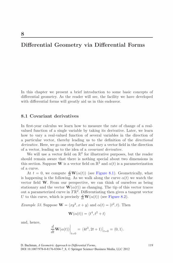
8
Differential Geometry via Differential Forms
In this chapter we present a brief introduction to some basic concepts ofdifferential geometry. As the reader will see, the facility we have developedwith differential forms will greatly aid us in this endeavor.
8.1 Covariant derivatives
In first-year calculus we learn how to measure the rate of change of a real-valued function of a single variable by taking its derivative. Later, we learnhow to vary a real-valued function of several variables in the direction ofa particular vector, thereby leading us to the definition of the directionalderivative. Here, we go one step further and vary a vector field in the directionof a vector, leading us to the idea of a covariant derivative.
We will use a vector field on R2 for illustrative purposes, but the reader
should remain aware that there is nothing special about two dimensions inthis section. Suppose W is a vector field on R
2 and α(t) is a parameterizationof a curve.
At t = 0, we compute ddtW(α(t)) (see Figure 8.1). Geometrically, what
is happening is the following. As we walk along the curve α(t) we watch thevector field W. From our perspective, we can think of ourselves as beingstationary and the vector W(α(t)) as changing. The tip of this vector tracesout a parameterized curve in TR2. Differentiating then gives a tangent vectorU to this curve, which is precisely d
dtW(α(t)) (see Figure 8.2).
Example 53. Suppose W = 〈xy2, x+ y〉 and α(t) = (t2, t). Then
W(α(t)) = 〈t4, t2 + t〉
and, hence,d
dtW(α(t))
∣∣∣∣t=0
= 〈4t3, 2t+ 1〉∣∣t=0
= 〈0, 1〉.
DOI 10.1007/978-0-8176-830 - _8, © Springer Science+Business Media, LLC 2012, D. Bachman
4 7119,A Geometric Approach to Differential Forms
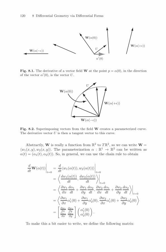
120 8 Differential Geometry via Differential Forms
W(α(−ε))
W(α(0))
W(α(+ε))U
α′(0)
Fig. 8.1. The derivative of a vector field W at the point p = α(0), in the directionof the vector α′(0), is the vector U .
W(α(−ε))
W(α(0))
W(α(+ε))
U
Fig. 8.2. Superimposing vectors from the field W creates a parameterized curve.The derivative vector U is then a tangent vector to this curve.
Abstractly, W is really a function from R2 to TR2, so we can write W =
〈w1(x, y), w2(x, y)〉. The parameterization α : R1 → R
2 can be written asα(t) = (α1(t), α2(t)). So, in general, we can use the chain rule to obtain
d
dtW(α(t))
∣∣∣∣t=0
=d
dt〈w1(α(t)), w2(α(t))〉
∣∣∣∣t=0
=
⟨dw1(α(t))
dt,dw2(α(t))
dt
⟩∣∣∣∣t=0
=
⟨∂w1
∂x
dα1
dt+∂w1
∂y
dα2
dt,∂w2
∂x
dα1
dt+∂w2
∂y
dα2
dt
⟩∣∣∣∣t=0
=
⟨∂w1
∂xα′1(0) +
∂w1
∂yα′2(0),
∂w2
∂xα′1(0) +
∂w2
∂yα′2(0)
⟩
=
[∂w1
∂x∂w1
∂y∂w2
∂x∂w2
∂y
](α′1(0)α′2(0)
).
To make this a bit easier to write, we define the following matrix:
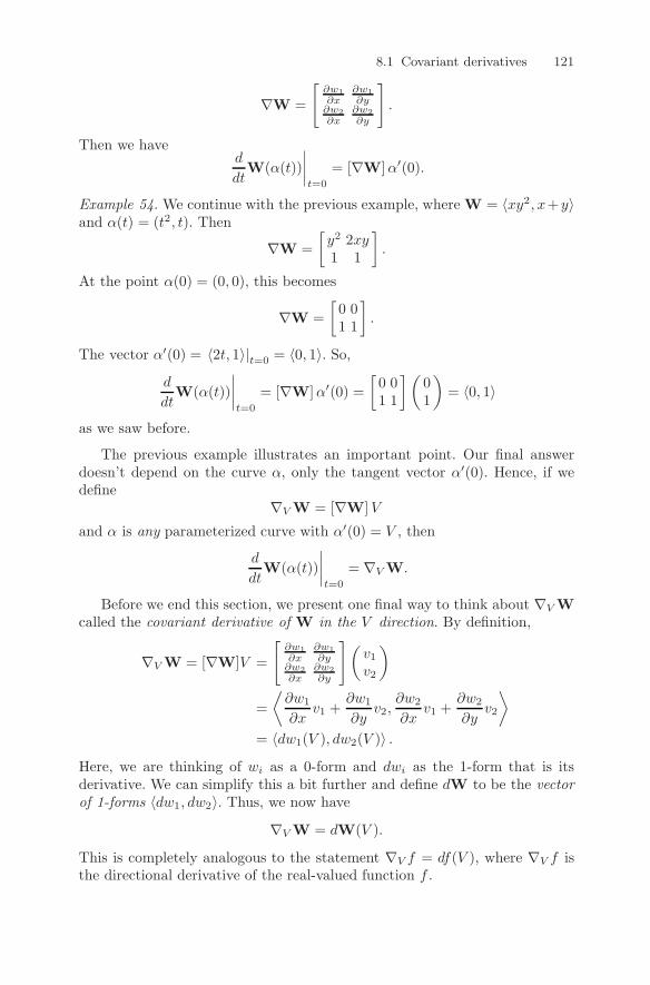
8.1 Covariant derivatives 121
∇W =
[∂w1
∂x∂w1
∂y∂w2
∂x∂w2
∂y
].
Then we haved
dtW(α(t))
∣∣∣∣t=0
= [∇W]α′(0).
Example 54. We continue with the previous example, where W = 〈xy2, x+y〉and α(t) = (t2, t). Then
∇W =
[y2 2xy1 1
].
At the point α(0) = (0, 0), this becomes
∇W =
[0 01 1
].
The vector α′(0) = 〈2t, 1〉|t=0 = 〈0, 1〉. So,d
dtW(α(t))
∣∣∣∣t=0
= [∇W]α′(0) =[0 01 1
](01
)= 〈0, 1〉
as we saw before.
The previous example illustrates an important point. Our final answerdoesn’t depend on the curve α, only the tangent vector α′(0). Hence, if wedefine
∇VW = [∇W]V
and α is any parameterized curve with α′(0) = V , then
d
dtW(α(t))
∣∣∣∣t=0
= ∇VW.
Before we end this section, we present one final way to think about ∇VWcalled the covariant derivative of W in the V direction. By definition,
∇VW = [∇W]V =
[∂w1
∂x∂w1
∂y∂w2
∂x∂w2
∂y
](v1v2
)
=
⟨∂w1
∂xv1 +
∂w1
∂yv2,
∂w2
∂xv1 +
∂w2
∂yv2
⟩= 〈dw1(V ), dw2(V )〉 .
Here, we are thinking of wi as a 0-form and dwi as the 1-form that is itsderivative. We can simplify this a bit further and define dW to be the vectorof 1-forms 〈dw1, dw2〉. Thus, we now have
∇VW = dW(V ).
This is completely analogous to the statement ∇V f = df(V ), where ∇V f isthe directional derivative of the real-valued function f .
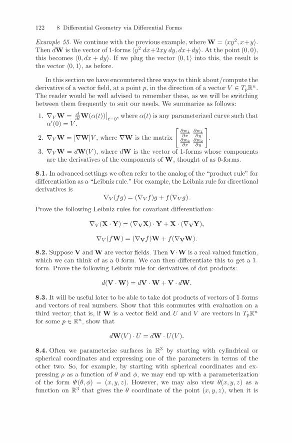
122 8 Differential Geometry via Differential Forms
Example 55. We continue with the previous example, where W = 〈xy2, x+y〉.Then dW is the vector of 1-forms 〈y2 dx+2xy dy, dx+dy〉. At the point (0, 0),this becomes 〈0, dx + dy〉. If we plug the vector 〈0, 1〉 into this, the result isthe vector 〈0, 1〉, as before.
In this section we have encountered three ways to think about/compute thederivative of a vector field, at a point p, in the direction of a vector V ∈ TpR
n.The reader would be well advised to remember these, as we will be switchingbetween them frequently to suit our needs. We summarize as follows:
1. ∇VW = ddtW(α(t))
∣∣t=0
, where α(t) is any parameterized curve such thatα′(0) = V .
2. ∇VW = [∇W]V , where ∇W is the matrix
[∂w1
∂x∂w1
∂y∂w2
∂x∂w2
∂y
].
3. ∇VW = dW(V ), where dW is the vector of 1-forms whose componentsare the derivatives of the components of W, thought of as 0-forms.
8.1. In advanced settings we often refer to the analog of the “product rule” fordifferentiation as a “Leibniz rule.” For example, the Leibniz rule for directionalderivatives is
∇V (fg) = (∇V f)g + f(∇V g).
Prove the following Leibniz rules for covariant differentiation:
∇V (X ·Y) = (∇VX) ·Y +X · (∇VY),
∇V (fW) = (∇Vf)W+ f(∇VW).
8.2. Suppose V and W are vector fields. ThenV ·W is a real-valued function,which we can think of as a 0-form. We can then differentiate this to get a 1-form. Prove the following Leibniz rule for derivatives of dot products:
d(V ·W) = dV ·W+V · dW.
8.3. It will be useful later to be able to take dot products of vectors of 1-formsand vectors of real numbers. Show that this commutes with evaluation on athird vector; that is, if W is a vector field and U and V are vectors in TpR
n
for some p ∈ Rn, show that
dW(V ) · U = dW · U(V ).
8.4. Often we parameterize surfaces in R3 by starting with cylindrical or
spherical coordinates and expressing one of the parameters in terms of theother two. So, for example, by starting with spherical coordinates and ex-pressing ρ as a function of θ and φ, we may end up with a parameterizationof the form Ψ(θ, φ) = (x, y, z). However, we may also view θ(x, y, z) as afunction on R
3 that gives the θ coordinate of the point (x, y, z), when it is
8.2 Frame fields and Gaussian curvature 123
expressed in spherical coordinates. Hence, it is often the case that we haveparameterizations of the form Ψ(θ, φ) such that
θ(Ψ(θ, φ)) = θ and φ(Ψ(θ, φ)) = φ.
When we think of θ(x, y, z) as a 0-form on R3, we can differentiate to get
a 1-form dθ. Show that
dθ
(∂Ψ
∂θ
)= dφ
(∂Ψ
∂φ
)= 1 and dθ
(∂Ψ
∂φ
)= dφ
(∂Ψ
∂θ
)= 0.
8.2 Frame fields and Gaussian curvature
Our approach to the subject of differential geometry loosely follows Cartan’smethod of moving frames. Roughly speaking, this involves a choice of a partic-ularly nice basis for the tangent space at each point of a surface S in R
n, calleda frame field. Geometric properties of S can then be derived from the way theframe field varies from one point to the next. This is where the language ofdifferential forms comes in handy.
Definition 3. Let S be a surface in R3. A frame field on S is a choice of
vector fields E1,E2 such that at each point p of S, E1(p) and E2(p) forman orthonormal basis for TpS.
The orthonormality condition is equivalent to
E1 · E2 = 0, E1 · E1 = E2 · E2 = 1.
Geometric properties of S follow from the way E1 and E2 vary from onepoint of S to the next. To this end, we now examine the covariant derivativesof E1 and E2. Let V be a tangent vector to S at some point. We can thentake the directional derivative of both sides of the equation
E1 · E1 = 1
to obtain∇V (E1 ·E1) = ∇V 1.
Using the appropriate Leibniz rule this becomes
(∇V E1) · E1 +E1 · (∇V E1) = 0.
and thus, (∇V E1) · E1 = 0. We conclude that ∇VE1 is a vector that isperpendicular to E1 and is thus in the plane spanned by E2 and the normalvector N to S.
Now, suppose S is a plane. Then a normal vector N to S is constant(i.e., it does not depend on a choice of p ∈ S). Since E1 is tangent to S, we
124 8 Differential Geometry via Differential Forms
have E1 ·N = 0. Again, taking the directional derivative of both sides of thisequation and applying the appropriate Leibniz rule gives us
(∇V E1) ·N +E1 · (∇VN) = 0.
However, since N is constant, ∇VN = 0. We conclude (∇V E1) ·N = 0, and,thus, when S is a plane, ∇V E1 is also perpendicular to N . We already knew∇V E1 was perpendicular to E1, so we may now conclude that ∇V E1 pointsin the same direction as E2.
Now, suppose for some surface S that the vector ∇V E1 does not point inthe same direction as E2 at a point p ∈ S. Then, near p, it must be the casethat S does not look like a plane (i.e., it has some curvature). This motivates usto look toward the projection of ∇V E1 onto E2 as a measure of the curvature(or lack thereof) of S. This projection is a linear function of the vector V andis thus a 1-form. We define
Ω(V ) = (∇V E1) ·E2.
Since (∇V E1) · E2 = dE1(V ) · E2 = dE1 · E2(V ), it is sometimes moreconvenient to write
Ω = dE1 ·E2.
We now define a numerical measure of the curvature of S at each point,which does not depend on a choice of tangent vector at that point.
Definition 4. The Gaussian curvature at each point of S is defined to be thenumber
K = −dΩ(E1,E2).
The amazing thing about the Gaussian curvature is that it is independentof the choice of frame field. It is a number that is completely determined bythe shape of S. We prove this now.
Theorem 3. At each point of S, the Gaussian curvature is independent ofthe choice of frame field.
Proof. Suppose E1 = 〈E11 , E
21 , E
31〉 and E2 = 〈E1
2 , E22 , E
32 〉. Then note that
dΩ = d(dE1 · E2)
= d(〈dE11 , dE
21 , dE
31〉 · 〈E1
2 , E22 , E
32〉)
= d(dE11E
12 + dE2
1E22 + dE3
1E32 )
= dE11 ∧ dE1
2 + dE21 ∧ dE2
2 + dE31 ∧ dE3
2 .
We can rewrite this more compactly using summation notation:
dΩ =
3∑i=1
dEi1 ∧ dEi2.
8.2 Frame fields and Gaussian curvature 125
Now, suppose F1,F2 is some other frame field on S. Let φ : S → R1
be the angle between E1 and F1. As any orthonormal basis can be obtainedfrom any other by rotation, it must be the case that
F1 = cosφE1 + sinφE2,
F2 = − sinφE1 + cosφE2.
Let Ω′ = dF1 · F2. Then the Gaussian curvature computed by using theframe field F1,F2 is given by evaluation of the 2-form dΩ′ on these twovectors. We now calculate
dΩ′ =3∑i=1
dF i1 ∧ dF i2
=
3∑i=1
d(cosφEi1 + sinφEi2) ∧ d(− sinφEi1 + cosφEi2)
=
3∑i=1
(− sinφEi1dφ+ cosφdEi1 + cosφEi2dφ+ sinφdEi2)
∧(− cosφEi1dφ− sinφdEi1 − sinφEi2dφ+ cosφdEi2)
=
3∑i=1
Ei1dφ ∧ dEi1 + Ei2dφ ∧ dEi2 + dEi1 ∧ dEi2
= dφ ∧(
3∑i=1
Ei1dEi1
)+ dφ ∧
(3∑i=1
Ei2dEi2
)+
3∑i=1
dEi1 ∧ dEi2
= dφ ∧ (E1 · dE1) + dφ ∧ (E2 · dE2) + dΩ.
Now, note that differentiating the equation E1 · E1 = 1 tells us thatE1 · dE1 = 0. Identical reasoning leads us to conclude E2 · dE2 = 0, and thuswe have dΩ′ = dΩ. Finally, note that since these 2-forms are the same, thenevaluating either one on any pair of vectors that span a parallelogram of areaone in a fixed plane will always produce the same number. Thus,
K ′ = dΩ′(F1,F2) = dΩ(E1,E2) = K,
as desired.
Example 56. We compute the Gaussian curvature of a sphere S of radius R.We begin by defining a frame field on it. As usual, a parameterization for Sis given by
Ψ(θ, φ) = (R sinφ cos θ,R sinφ sin θ,R cosφ).
The partial derivatives of this give tangent vectors to S:
126 8 Differential Geometry via Differential Forms
∂Ψ
∂θ= 〈−R sinφ sin θ,R sinφ cos θ, 0〉,
∂Ψ
∂φ= 〈R cosφ cos θ,R cosφ sin θ,−R sinφ〉.
Since the dot product of these two vectors is zero, they are orthogonal. Toget a frame field then, we must simply divide each vector by its magnitude toget unit vectors:
E1 =1
R sinφ
∂Ψ
∂θ= 〈− sin θ, cos θ, 0〉,
E2 =1
R
∂Ψ
∂φ= 〈cosφ cos θ, cosφ sin θ,− sinφ〉.
Now, we find the 1-form Ω. Since
dE1 = 〈− cos θ dθ,− sin θ dθ, 0〉,we have
Ω = dE1 · E2 = − cosφ cos2 θ dθ − cosφ sin2 θ dθ = − cosφ dθ.
Thus,−dΩ = − sinφ dφ ∧ dθ.
To compute K = −dΩ(E1,E2), we will need to know the following:
dθ(E1) = dθ
(1
R sinφ
∂Ψ
∂θ
)=
1
R sinφdθ
(∂Ψ
∂θ
)=
1
R sinφ,
dφ(E1) = dφ
(1
R sinφ
∂Ψ
∂θ
)=
1
R sinφdφ
(∂Ψ
∂θ
)= 0,
dθ(E2) = dθ
(1
R
∂Ψ
∂φ
)=
1
Rdθ
(∂Ψ
∂φ
)= 0,
dφ(E2) = dφ
(1
R
∂Ψ
∂φ
)=
1
Rdφ
(∂Ψ
∂φ
)=
1
R.
We are now prepared to compute the Gaussian curvature:
K = −dΩ(E1,E2)
= − sinφ dφ ∧ dθ(E1,E2)
= − sinφ
∣∣∣∣dφ(E1) dθ(E1)dφ(E2) dθ(E2)
∣∣∣∣= − sinφ
∣∣∣∣ 0 1R sinφ
1R 0
∣∣∣∣= sinφ
1
R2 sinφ
=1
R2.
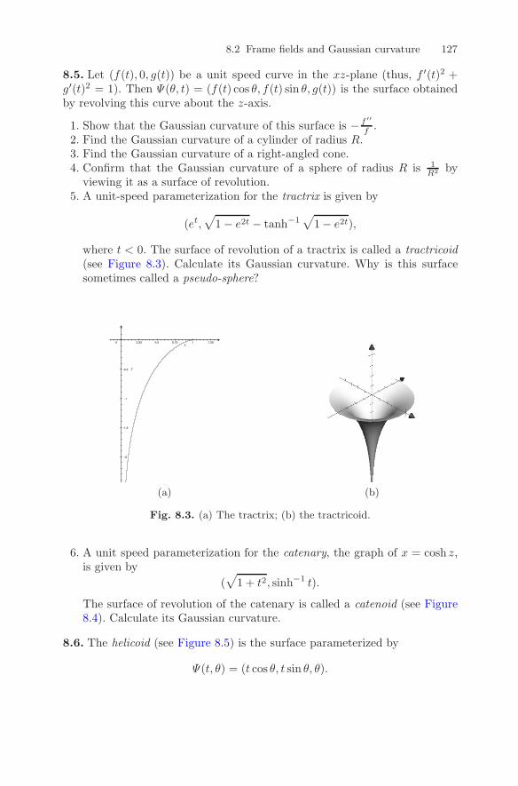
8.2 Frame fields and Gaussian curvature 127
8.5. Let (f(t), 0, g(t)) be a unit speed curve in the xz-plane (thus, f ′(t)2 +g′(t)2 = 1). Then Ψ(θ, t) = (f(t) cos θ, f(t) sin θ, g(t)) is the surface obtainedby revolving this curve about the z-axis.
1. Show that the Gaussian curvature of this surface is − f ′′
f .2. Find the Gaussian curvature of a cylinder of radius R.3. Find the Gaussian curvature of a right-angled cone.4. Confirm that the Gaussian curvature of a sphere of radius R is 1
R2 byviewing it as a surface of revolution.
5. A unit-speed parameterization for the tractrix is given by
(et,√1− e2t − tanh−1
√1− e2t),
where t < 0. The surface of revolution of a tractrix is called a tractricoid(see Figure 8.3). Calculate its Gaussian curvature. Why is this surfacesometimes called a pseudo-sphere?
0 0.25 0.5 0.75 1 1.25
-2
-1.5
-1
-0.5
(a) (b)
Fig. 8.3. (a) The tractrix; (b) the tractricoid.
6. A unit speed parameterization for the catenary, the graph of x = cosh z,is given by
(√
1 + t2, sinh−1 t).
The surface of revolution of the catenary is called a catenoid (see Figure8.4). Calculate its Gaussian curvature.
8.6. The helicoid (see Figure 8.5) is the surface parameterized by
Ψ(t, θ) = (t cos θ, t sin θ, θ).
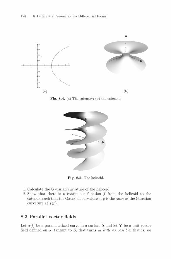
128 8 Differential Geometry via Differential Forms
-1 -0.5 0 0.5 1 1.5 2 2.5 3 3.5
-1 6
-1.2
-0.8
-0.4
0.4
0.8
1.2
1.6
(a) (b)
Fig. 8.4. (a) The catenary; (b) the catenoid.
Fig. 8.5. The helicoid.
1. Calculate the Gaussian curvature of the helicoid.2. Show that there is a continuous function f from the helicoid to the
catenoid such that the Gaussian curvature at p is the same as the Gaussiancurvature at f(p).
8.3 Parallel vector fields
Let α(t) be a parameterized curve in a surface S and let Y be a unit vectorfield defined on α, tangent to S, that turns as little as possible; that is, we
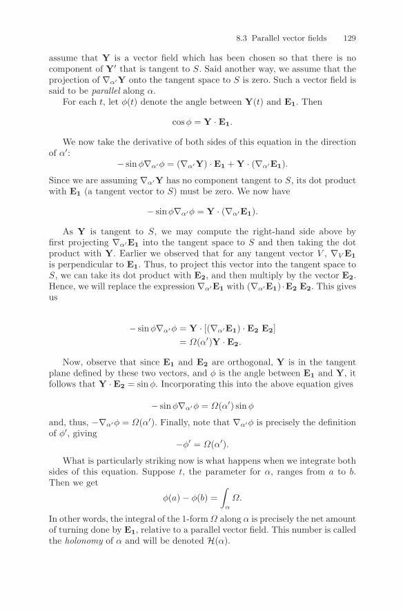
8.3 Parallel vector fields 129
assume that Y is a vector field which has been chosen so that there is nocomponent of Y′ that is tangent to S. Said another way, we assume that theprojection of ∇α′Y onto the tangent space to S is zero. Such a vector field issaid to be parallel along α.
For each t, let φ(t) denote the angle between Y(t) and E1. Then
cosφ = Y · E1.
We now take the derivative of both sides of this equation in the directionof α′:
− sinφ∇α′φ = (∇α′Y) ·E1 +Y · (∇α′E1).
Since we are assuming ∇α′Y has no component tangent to S, its dot productwith E1 (a tangent vector to S) must be zero. We now have
− sinφ∇α′φ = Y · (∇α′E1).
As Y is tangent to S, we may compute the right-hand side above byfirst projecting ∇α′E1 into the tangent space to S and then taking the dotproduct with Y. Earlier we observed that for any tangent vector V , ∇V E1
is perpendicular to E1. Thus, to project this vector into the tangent space toS, we can take its dot product with E2, and then multiply by the vector E2.Hence, we will replace the expression ∇α′E1 with (∇α′E1) ·E2 E2. This givesus
− sinφ∇α′φ = Y · [(∇α′E1) · E2 E2]
= Ω(α′)Y ·E2.
Now, observe that since E1 and E2 are orthogonal, Y is in the tangentplane defined by these two vectors, and φ is the angle between E1 and Y, itfollows that Y ·E2 = sinφ. Incorporating this into the above equation gives
− sinφ∇α′φ = Ω(α′) sinφ
and, thus, −∇α′φ = Ω(α′). Finally, note that ∇α′φ is precisely the definitionof φ′, giving
−φ′ = Ω(α′).
What is particularly striking now is what happens when we integrate bothsides of this equation. Suppose t, the parameter for α, ranges from a to b.Then we get
φ(a)− φ(b) =
∫α
Ω.
In other words, the integral of the 1-formΩ along α is precisely the net amountof turning done by E1, relative to a parallel vector field. This number is calledthe holonomy of α and will be denoted H(α).
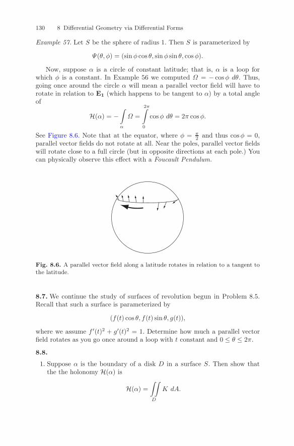
130 8 Differential Geometry via Differential Forms
Example 57. Let S be the sphere of radius 1. Then S is parameterized by
Ψ(θ, φ) = (sinφ cos θ, sinφ sin θ, cosφ).
Now, suppose α is a circle of constant latitude; that is, α is a loop forwhich φ is a constant. In Example 56 we computed Ω = − cosφ dθ. Thus,going once around the circle α will mean a parallel vector field will have torotate in relation to E1 (which happens to be tangent to α) by a total angleof
H(α) = −∫α
Ω =
2π∫0
cosφ dθ = 2π cosφ.
See Figure 8.6. Note that at the equator, where φ = π2 and thus cosφ = 0,
parallel vector fields do not rotate at all. Near the poles, parallel vector fieldswill rotate close to a full circle (but in opposite directions at each pole.) Youcan physically observe this effect with a Foucault Pendulum.
Fig. 8.6. A parallel vector field along a latitude rotates in relation to a tangent tothe latitude.
8.7. We continue the study of surfaces of revolution begun in Problem 8.5.Recall that such a surface is parameterized by
(f(t) cos θ, f(t) sin θ, g(t)),
where we assume f ′(t)2 + g′(t)2 = 1. Determine how much a parallel vectorfield rotates as you go once around a loop with t constant and 0 ≤ θ ≤ 2π.
8.8.
1. Suppose α is the boundary of a disk D in a surface S. Then show thatthe the holonomy H(α) is
H(α) =
∫∫D
K dA.
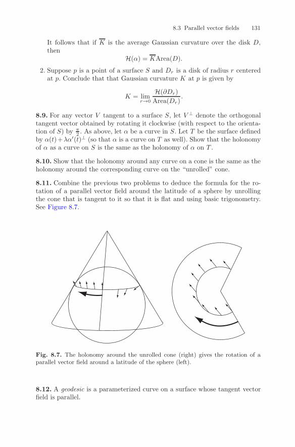
8.3 Parallel vector fields 131
It follows that if K is the average Gaussian curvature over the disk D,then
H(α) = KArea(D).
2. Suppose p is a point of a surface S and Dr is a disk of radius r centeredat p. Conclude that that Gaussian curvature K at p is given by
K = limr→0
H(∂Dr)
Area(Dr).
8.9. For any vector V tangent to a surface S, let V ⊥ denote the orthogonaltangent vector obtained by rotating it clockwise (with respect to the orienta-tion of S) by π
2 . As above, let α be a curve in S. Let T be the surface definedby α(t)+λα′(t)⊥ (so that α is a curve on T as well). Show that the holonomyof α as a curve on S is the same as the holonomy of α on T .
8.10. Show that the holonomy around any curve on a cone is the same as theholonomy around the corresponding curve on the “unrolled” cone.
8.11. Combine the previous two problems to deduce the formula for the ro-tation of a parallel vector field around the latitude of a sphere by unrollingthe cone that is tangent to it so that it is flat and using basic trigonometry.See Figure 8.7.
Fig. 8.7. The holonomy around the unrolled cone (right) gives the rotation of aparallel vector field around a latitude of the sphere (left).
8.12. A geodesic is a parameterized curve on a surface whose tangent vectorfield is parallel.
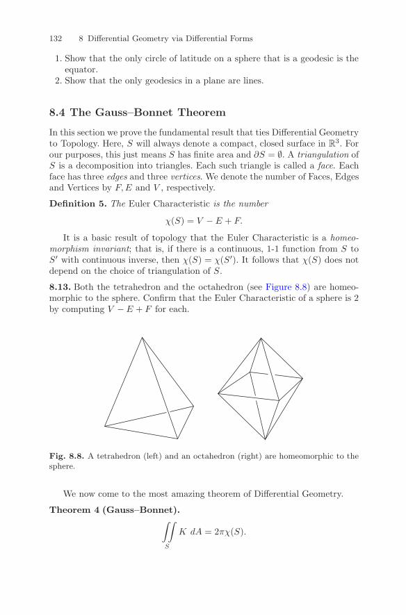
132 8 Differential Geometry via Differential Forms
1. Show that the only circle of latitude on a sphere that is a geodesic is theequator.
2. Show that the only geodesics in a plane are lines.
8.4 The Gauss–Bonnet Theorem
In this section we prove the fundamental result that ties Differential Geometryto Topology. Here, S will always denote a compact, closed surface in R
3. Forour purposes, this just means S has finite area and ∂S = ∅. A triangulation ofS is a decomposition into triangles. Each such triangle is called a face. Eachface has three edges and three vertices. We denote the number of Faces, Edgesand Vertices by F,E and V , respectively.
Definition 5. The Euler Characteristic is the number
χ(S) = V − E + F.
It is a basic result of topology that the Euler Characteristic is a homeo-morphism invariant; that is, if there is a continuous, 1-1 function from S toS′ with continuous inverse, then χ(S) = χ(S′). It follows that χ(S) does notdepend on the choice of triangulation of S.
8.13. Both the tetrahedron and the octahedron (see Figure 8.8) are homeo-morphic to the sphere. Confirm that the Euler Characteristic of a sphere is 2by computing V − E + F for each.
Fig. 8.8. A tetrahedron (left) and an octahedron (right) are homeomorphic to thesphere.
We now come to the most amazing theorem of Differential Geometry.
Theorem 4 (Gauss–Bonnet).∫∫S
K dA = 2πχ(S).
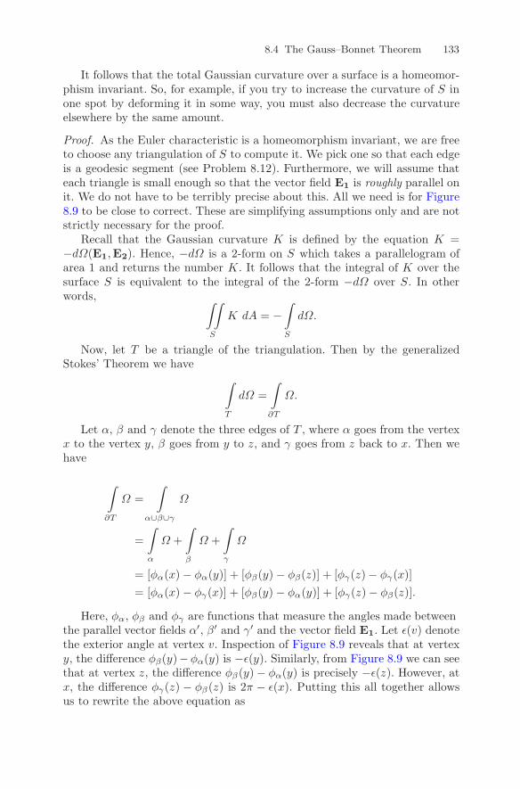
8.4 The Gauss–Bonnet Theorem 133
It follows that the total Gaussian curvature over a surface is a homeomor-phism invariant. So, for example, if you try to increase the curvature of S inone spot by deforming it in some way, you must also decrease the curvatureelsewhere by the same amount.
Proof. As the Euler characteristic is a homeomorphism invariant, we are freeto choose any triangulation of S to compute it. We pick one so that each edgeis a geodesic segment (see Problem 8.12). Furthermore, we will assume thateach triangle is small enough so that the vector field E1 is roughly parallel onit. We do not have to be terribly precise about this. All we need is for Figure8.9 to be close to correct. These are simplifying assumptions only and are notstrictly necessary for the proof.
Recall that the Gaussian curvature K is defined by the equation K =−dΩ(E1,E2). Hence, −dΩ is a 2-form on S which takes a parallelogram ofarea 1 and returns the number K. It follows that the integral of K over thesurface S is equivalent to the integral of the 2-form −dΩ over S. In otherwords, ∫∫
S
K dA = −∫S
dΩ.
Now, let T be a triangle of the triangulation. Then by the generalizedStokes’ Theorem we have ∫
T
dΩ =
∫∂T
Ω.
Let α, β and γ denote the three edges of T , where α goes from the vertexx to the vertex y, β goes from y to z, and γ goes from z back to x. Then wehave
∫∂T
Ω =
∫α∪β∪γ
Ω
=
∫α
Ω +
∫β
Ω +
∫γ
Ω
= [φα(x)− φα(y)] + [φβ(y)− φβ(z)] + [φγ(z)− φγ(x)]
= [φα(x)− φγ(x)] + [φβ(y)− φα(y)] + [φγ(z)− φβ(z)].
Here, φα, φβ and φγ are functions that measure the angles made betweenthe parallel vector fields α′, β′ and γ′ and the vector field E1. Let ε(v) denotethe exterior angle at vertex v. Inspection of Figure 8.9 reveals that at vertexy, the difference φβ(y)−φα(y) is −ε(y). Similarly, from Figure 8.9 we can seethat at vertex z, the difference φβ(y)− φα(y) is precisely −ε(z). However, atx, the difference φγ(z) − φβ(z) is 2π − ε(x). Putting this all together allowsus to rewrite the above equation as
134 8 Differential Geometry via Differential Forms
E1E1
E1
x
y
z
α
β
γ
+
+
+
−
−
−
α′
γ′
β′
α′
γ′
φγ(z)− φβ(z)
φβ(y)− φα(y)
φβ(y)− φα(y)
β′
Fig. 8.9. At vertex y, the difference between the angle made by β′ and E1 andthe angle made by α′ and E1 is the negative of the exterior angle ε(y). Similarly, atvertex z, the difference is −ε(z). However, at x, the difference is 2π − ε(x).
∫∂T
Ω = 2π − ε(x) − ε(y)− ε(z).
It will be more convenient to express this in terms of the interior angles.Let ι(v) denote the interior angle at v. Then ε(v) = π − ι(v). Thus, we nowhave ∫
∂T
Ω = −π + ι(x) + ι(y) + ι(z).
Now, we add over all triangles. Around each vertex we end up addingall of the interior angles and therefore get 2π. Hence, when we sum over alltriangles, the sum of all interior angles is just 2πV . We also add −π for eachtriangle, so this sum is −πF . Putting everything together thus gives us
8.4 The Gauss–Bonnet Theorem 135∫∫S
K dA = −∫S
dΩ
= −F∑i=1
∫Ti
dΩ
= −F∑i=1
∫∂Ti
Ω
= πF − 2πV.
Now, notice that every triangle has three edges, but these edges are countedtwice when we sum over all triangles. Hence, E = 3
2F , or 2E = 3F . This allowsus to rewrite the above as
∫∫S
K dA = πF − 2πV
= −2πF + 3πF − 2πV
= −2πF + 2πE − 2πV
= −2πχ(S).
8.14. Show by direct computation that the integral of the Gaussian curvatureover a sphere of radius R is −4π.
8.15. Derive the formula for the area of a sphere of radius R from the Gauss–Bonnet Theorem and the fact that the Euler Characteristic of a sphere is2.
8.16. A geodesic triangle is a triangle in a surface whose sides are geodesics.Find formulas for the area of geodesic triangles on a sphere of radius 1 anda pseudo-sphere (whose Gaussian curvature is −1) in terms of their interiorangles. Why can’t you find such a formula for geodesic triangles in a plane?What can you conclude about the sum of the angles of a geodesic triangle,compared to π, on a sphere, plane and psuedo-sphere?
8.17. Let α(t) be a unit-speed parameterization of a simple, closed curve inR
3, where a ≤ t ≤ b. Let T = α′, N be a unit vector pointing in the directionof α′′, and B = T ×N . Let S be the surface parameterized by
Ψ(t, θ) = α(t) + cos θN(t) + sin θB(t),
where a ≤ t ≤ b and 0 ≤ θ ≤ 2π.
1. Describe S.2. Show that at the point Ψ(t, θ), the vectors E1 = T (t) and E2 = ∂Ψ
∂θ areorthogonal unit tangent vectors to S and thus form a frame field.
136 8 Differential Geometry via Differential Forms
3. Compute the Gaussian curvature of S.4. Compute the holonomy of a loop on S where a ≤ t ≤ b and θ is fixed.5. Compute the total Gaussian curvature of S by integration.6. What can you conclude about the Euler Characteristic of S?
References
[Arn97] V. I. Arnol′d. Mathematical Methods of Classical Mechanics, volume 60 ofGraduate Texts in Mathematics. Springer-Verlag, New York, 1997. Trans-lated from the 1974 Russian original by K. Vogtmann and A. Weinstein,Corrected reprint of the second (1989) edition.
[BT82] Raoul Bott and Loring W. Tu. Differential Forms in Algebraic Topology,volume 82 of Graduate Texts in Mathematics. Springer-Verlag, New York,1982.
[GP10] Victor Guillemin and Alan Pollack. Differential Topology. AMS ChelseaPublishing, Providence, RI, 2010. Reprint of the 1974 original.
[HH99] John Hamal Hubbard and Barbara Burke Hubbard. Vector Calculus,Linear Algebra, and Differential Forms. Prentice Hall Inc., Upper SaddleRiver, NJ, 1999. A unified approach.
[MTW73] Charles W. Misner, Kip S. Thorne, and John Archibald Wheeler. Grav-itation. W. H. Freeman and Co., San Francisco, Calif., 1973.
DOI 10.1007/978-0-8176-830 - , © Springer Science+Business Media, LLC 2012, D. Bachman
4 7137,A Geometric Approach to Differential Forms

Books For Further Reading
[1] R. W. R. Darling. Differential Forms and Connections. Cambridge UniversityPress, Cambridge, 1994.
[2] Manfredo P. do Carmo. Differential Forms and Applications. Universitext.Springer-Verlag, Berlin, 1994. Translated from the 1971 Portuguese original.
[3] Harley Flanders. Differential Forms with Applications to the Physical Sciences.Dover Books on Advanced Mathematics. Dover Publications Inc., New York,second edition, 1989.
[4] Barrett O’Neill. Elementary Differential Geometry. Elsevier/Academic Press,Amsterdam, second edition, 2006.
[5] Michael Spivak. Calculus on Manifolds. A Modern Approach to Classical Theo-rems of Advanced Calculus. W. A. Benjamin, Inc., New York-Amsterdam, 1965.
139

Index
4-current, 99
alternating, 38, 73, 74, 104antiderivative, 77, 115arc length, 1, 3, 69area form, 39, 114
bilinear, 31, 33, 47boundary, 84–86
Cartan’s method of moving frames, seemethod of moving frames
catenary, 127, 128catenoid, 127, 128cell, 83
boundary of, 84, 85chain, 83change of variables formula, 57, 58charge density, 99closed
chain, 103, 104, 107, 110–113curve, 96, 135form, 103, 110, 111, 115subset, 107surface, 132
cohomology, 112, 115contact structure, 77coordinate-free, 78, 100covariant derivative, 119, 121–123cover, 106, 108covering map, 106cross product, 36, 67curl, 93, 94current density, 99
cylindrical coordinates, 14
DeRham Cohomology, 110derivative
notation, 26of a differential form, 71of a multivariable function, see
directional derivativeof a parameterization, 17, 18, 21, 54,
55, 108of a single-variable function, 4, 119of a vector field, see covariant
derivativedescend, 106, 107determinant, 57, 65differential form, 1, 41differential geometry, 119, 123, 132dimension, 104, 108directional derivative, 10, 12–13, 71,
119, 121–124discrete action, 107div, 94dot product, 12, 27, 122, 126, 129
equivalence relation, 106, 111, 112Euler Characteristic, 132, 133, 135, 136exact form, 111, 112, 115
Faraday, 99foliation, 77, 80, 81, 116Foucault Pendulum, 130frame field, 123, 135frustrum, 52Fubini’s Theorem, 44, 59
141
142 Index
fundamental domain, 107Fundamental Theorem of Calculus, 93
Gauss’ Divergence Theorem, 98Gauss, Carl Friedrich, 114Gauss–Bonnet Theorem, 132Gaussian curvature, 123, 131, 133, 135,
136geodesic, 131, 133
triangle, 135Godbillon–Vey Invariant, 116grad, 93gradient, 10, 71
field, 96vector, 13
Green’s Theorem, 93group, 107
helicoid, 127, 128holonomy, 129–131, 136homeomorphism, 106, 132
invariant, 132, 133homotopy invariant, 115Hopf Invariant, 115, 116, 117Hopf, Heinz, 115
kernel, 78–81, 116knot, 112, 113, 116
latitude, 13, 130–132lattice, 5, 43–47, 86Legendrian curve, 81Leibniz rule, 122–124length form, 113level curve, 13lift, 106line field, 78line integral, 69, 96linear algebra, 38, 78linear function, 1, 5, 67link, 112–114linking number, 112, 116longitude, 13
manifold, 101, 112Maxwell, 99Maxwell’s Equations, 98measure zero, 107method of moving frames, 123
multilinear, 38, 73, 104multivariable calculus, 7
neighborhood, 79
octahedron, 132open set, 77, 103, 105, 106, 108, 110orientation, 45, 50
induced, 52of a cell, 83of a point, 83
orthonormal basis, 123, 125
parallel vector field, 128, 133parallelepiped, 37–39, 116parameterized
cell, 90, 91curve, 16, 21, 53–55, 69, 79, 89, 95,
113, 119–122, 128, 131line, 16manifold, 108region, 6, 21, 53, 56, 60, 62, 63, 75,
83, 88, 97, 104surface, 19, 41, 44, 46, 49, 52, 53,
95–97, 127, 130, 135partition of unity, 109–110plane field, 77–81, 116pseudo-sphere, 127, 135pull-back, 101, 108, 109, 113–115
Reeb Foliation, 80, 82Riemann Sum, 3, 5, 6, 46, 48, 87
scalar, 32, 34, 35second partial, 8signed area, 30, 33skew-symmetric, 31, 33spherical coordinates, 14Stokes’ Theorem, 86
classical, 97generalized, 87, 103, 133
substitution rule, 57surface
area, 1, 67, 67, 68integral, 68, 98of revolution, 127, 130
tangentcone, 131line, 8, 10–13, 17, 25, 26, 74, 108
Index 143
plane, 10–11, 21, 74, 77–80, 104, 116,129
space, 25–26, 53, 77, 108, 123, 129
vector, 5, 18, 21, 25, 51, 54, 64–66,95, 113, 114, 119–121, 123–125,131
vector field, 128, 129, 131, 135
tetrahedron, 132
topology, 103, 105, 107, 112, 132
algebraic, 112, 115
differential, 109
torus, 7, 80, 82, 107
tractricoid, 127
tractrix, 127transformation, 107triangulation, 132, 133trigonometric substitution, 57
u-substitution, 57
vector calculus, 35, 92vector field, 42, 71, 73, 93–99, 119, 120,
122, 128–131, 133volume form, 39, 57
wedge product, 29–31, 37, 38, 74winding number, 104, 106, 113

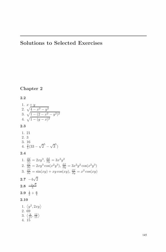
Solutions to Selected Exercises
Chapter 2
2.2
1. x+ y2.
√4− x2 − y2
3.√1− (2− x2 − y2)2
4.√1− (y − x)2
2.3
1. 212. 33. 164. 2
5 (33−√25 −√
35)
2.4
1. ∂f∂x = 2xy3, ∂f∂y = 3x2y2
2. ∂f∂x = 2xy3 cos(x2y3), ∂f∂y = 3x2y2 cos(x2y3)
3. ∂f∂x = sin(xy) + xy cos(xy), ∂f∂y = x2 cos(xy)
2.7 −4√2
2.8 −2√5
5
2.9 12 + π
4
2.10
1.⟨y2, 2xy
⟩2. 693.
⟨915 ,
1215
⟩4. 15
145
146
2.11 5
2.13r = ρ sinφ ρ =
√r2 + z2
θ = θ θ = θz = ρ cosφ φ = tan−1
(rz
)2.15
1. z =√x2 + y2, z = r, φ = π
42. y = 0, θ = 0, θ = 03. z = 0, z = 0, φ = π
24. z = x+ y, z = r(sin θ + cos θ), cotφ = sin θ + cos θ
5. z = (x2 + y2)32 , z = r
32 , z = (ρ sinφ)
32
2.16
1. S is the top half of a “two-sheeted hyperboloid.” You can see it as thesurface obtained from the graph of z =
√x2 + 1 (in the xz-plane) by
rotating it around the z-axis.2. z =
√x2 + y2 + 1
2.17
1. ba
2. They are parallel. The one parameterized by φ can be obtained from theother by shifting c units to the right and d units up.
2.19
1. (cos2 θ, cos θ sin θ)2. (x, sin x)
2.20 φ(t) = (t, 4t− 3), 1 ≤ t ≤ 2 (There are many other answers.)
2.22
1. (t2, t)2. 〈4, 1〉2.24
1. The x-axis2. The z-axis3. The line y = z and x = 04. The line x = y = z
2.25 φ(t) = (t, 1− t,√1− 2t+ 2t2)
2.26
1. φ(θ) = (2 cos θ, 2 sin θ, 4), 0 ≤ θ ≤ 2π2. ψ(t) = (t,±√
4− t2, 4), −2 ≤ t ≤ 2
Solutions to Selected Exercises
147
2.27 Ψ(θ) = (sin θ cos θ, sin2 θ, cos θ)
2.28
1. φ(u, z) = (u, u, z)2. φ(r, θ) = (r cos θ, r sin θ, r2)3. ψ(θ, φ) = (φ sin φ cos θ, φ sinφ sin θ, φ cosφ)4. ψ(θ, φ) = (cosφ sin φ cos θ, cosφ sinφ sin θ, cosφ cosφ)5. φ(θ, z) = (cos2 θ, sin θ cos θ, z)6. φ(r, θ) = (r cos θ, r sin θ,
√r2 − 1)
7. φ(r, θ) = (r cos θ, r sin θ,√r2 + 1)
8. φ(θ, z) = (θ cos θ, θ sin θ, z)
2.29 φ(x, y) = (x, y, f(x, y))
2.30
1. Ψ(x, y) = (x, y, 4 − x2 − y2), 0 ≤ x ≤ 1, 0 ≤ y ≤ 12. Ψ(r, θ) = (r cos θ, r sin θ, 4− r2), 0 ≤ r ≤ 1, 0 ≤ θ ≤ 2π
2.32 ψ(θ, φ) = (2 sinφ cos θ, 2 sinφ sin θ, 2 cosφ), 0 ≤ θ ≤ 2π, π4 ≤ φ ≤ π2
2.34 〈2, 0, 4〉, 〈0, 3, 2〉2.36
1. ψ(ρ, θ, φ) = (ρ sinφ cos θ, ρ sinφ sin θ, ρ cosφ), 0 ≤ ρ ≤ 1, 0 ≤ θ ≤ 2π,0 ≤ φ ≤ π
2. ψ(ρ, θ, φ) = (ρ sinφ cos θ, ρ sinφ sin θ, ρ cosφ), 0 ≤ ρ ≤ 1, 0 ≤ θ ≤ π2 ,
0 ≤ φ ≤ π2
3. ψ(ρ, θ, φ) = (ρ sinφ cos θ, ρ sinφ sin θ, ρ cosφ), 0 ≤ ρ ≤ 1, π ≤ θ ≤ 3π2 ,
π2 ≤ φ ≤ π
2.37
1. φ(r, θ, z) = (r cos θ, r sin θ, z), 0 ≤ r ≤ 1, 0 ≤ θ ≤ 2π, 0 ≤ z ≤ 12. φ(r, θ, z) = (r cos θ, r sin θ, z), 1 ≤ r ≤ 2, 0 ≤ θ ≤ 2π, 0 ≤ z ≤ 2
2.38
φ(t, θ) = ([tf2(θ) + (1 − t)f1(θ)] cos θ, [tf2(θ) + (1− t)f1(θ)] sin θ),
0 ≤ t ≤ 1, a ≤ θ ≤ b
2.39 φ(r, θ) = (3r cos θ, 2r sin θ), 0 ≤ r ≤ 1, 0 ≤ θ ≤ 2π
Chapter 3
3.2
1. −1, 4, 10
Solutions to Selected Exercises
148
2. dy = −4dx
3.3
1. 3dx2. 1
2dy3. 3dx+ 1
2dy4. 8dx+ 6dy
3.5
1. ω(V1) = −8, ν(V1) = 1, ω(V2) = −1 and ν(V2) = 2.2. −153. 5
3.15 −127
3.16 c1 = −11, c2 = 4 and c3 = 3
3.17
1. 2dx ∧ dy2. dx ∧ (dy + dz)3. dx ∧ (2dy + dz)4. (dx + 3dz) ∧ (dy + 4dz)
3.27 4
3.28 8
3.31 252
3.32
1. −872. −293. 5
3.33 dx ∧ dy ∧ dz3.34
1. −2dx ∧ dy ∧ dz2. −2
3.36
1. z(x− y)dz ∧ dx+ z(x+ y)dz ∧ dy2. −4dx ∧ dy ∧ dz
Solutions to Selected Exercises
149
Chapter 4
4.1
1. 〈2, 3, 1〉,〈2, 3, 2〉2. 6dx ∧ dy + 3dy ∧ dz − 2dx ∧ dz3. 54. x2yz2 − x5z2 − y3 + x3y2
4.2 16
4.3
1. a) 4πb) −4π (Don’t worry that the sign is not the same as in the previous part.
Right now you really don’t have enough information yet to properlytell what the right sign should be.)
2. 4π3. 4
√2π
4.4 13
4.5
1. − 1712
2. − 296
4.6 18
4.7 64
4.9 3π5
4.10 16
4.11 14π3
4.12
1. Opposite orientation2. Same orientation3. Does not determine an orientation
4.13 83
4.14 16
4.15 16
4.16 15
4.17 23 cos 6− 3
2 sin 4− 23
4.18 16
4.19 4
Solutions to Selected Exercises
150
4.20 323
4.22 2
4.23 6π
4.25 12
4.26 143
4.27 −7π6
4.28 π3
(23/2 − 1
)4.29 2π
4.30 2π3
4.31
1. 13
2. π4
Chapter 5
5.1
1. ∇V ω(W ) = −62, ∇Wω(V ) = 42. −66
5.3 dω = (−2x− 1)dx ∧ dy5.6 d(x2y dx ∧ dy + y2z dy ∧ dz) = 0
5.7 −1, 1, 1
5.11 (3x4y2 − 4xy6z)dx ∧ dy ∧ dz5.12
1. 2x sin(y − z)dx+ x2 cos(y − z)dy − x2 cos(y − z)dz2. (− sinx− cos y)dx ∧ dy3. (z − x)dx ∧ dy + yz dx ∧ dz + x(z − 1)dy ∧ dz4. (3x2z − 2xy)dx ∧ dy − (x3 + 1)dy ∧ dz5. (2xz + z2)dx ∧ dy ∧ dz6. (2x+ 2y)dx ∧ dy ∧ dz7. (y2 − 9z8)dx ∧ dy ∧ dz8. 0
5.13(∂f∂x + ∂g
∂y + ∂h∂z
)dx ∧ dy ∧ dz
5.14
1. x dy
Solutions to Selected Exercises
151
2. x dy ∧ dz3. xyz4. xy2z2
5. sin(xy2)dx+ sin(xy2)dy
Chapter 6
6.1
1. 2, −22. 1
6.4 A circle of radius 1, centered on the z-axis, and one unit above thexy-plane. The orientation is in the direction of increasing θ.
6.12
1. 322. 1
6.13 12
6.14 2
6.15 27
6.16 353
6.17
1. 02.
∫C1
ω =∫C2
ω = 13
3. − 23
6.18
1. 02. 03. If L,R, T and B represent the 1-cells that are the left, right, top and
bottom of Q, respectively, then∫∂Q
ω =
∫(R−L)−(T−B)
ω =
∫R
ω−∫L
ω−∫T
ω+
∫B
ω = 24−0−281
2+4
1
2= 0
4. Opposite5. 4 1
26. 4 1
2
Solutions to Selected Exercises
152
6.19 8π
6.20 6π
6.21 23
(e− 1
e
)6.23 π
6.24 45π4
6.28 0
6.29
1. 〈1, 0, 0〉2. α = dy ∧ dz3. − 2
3
6.30 43
Chapter 7
7.1 −b3c da ∧ dc+ (a2 − ab2c)db ∧ dc7.8 φ∗τ = − b
a2+b2 da+a
a2+b2 db. This is the form on R2− (0, 0) that gives the
winding number around the origin, so τ measures how many times a curvewraps around the cylinder L.
7.9 dτ ′ = 2 dx ∧ dy and dτ = 0
Chapter 8
8.4 A geometric argument is easiest (and most insightful) here. The 1-form dθprojects vectors onto the vector∇θ, which points in the direction of increasingθ. The vector ∂Ψ
∂θ is found by starting at a point on the surface and moving inthe direction of increasing θ. This is precisely the same as the vector∇θ at thatpoint, so the projection is 1. Similarly, the 1-form dφ projects vectors onto∇φ.However, since ∇θ and ∇φ are orthogonal, we have dφ
(∂Ψ∂θ
)= dφ(∇θ) = 0.
8.5
1. A frame field is given by
E1 =1
f
∂Ψ
∂θ= 〈− sin θ, cos θ, 0〉,
E2 =∂Ψ
∂t= 〈f ′(t) cos θ, f ′(t) sin θ, g′(t)〉.
Thus,
Solutions to Selected Exercises
153
Ω = dE1 · E2
= 〈− cos θdθ,− sin θdθ, 0〉 · 〈f ′(t) cos θ, f ′(t) sin θ, g′(t)〉= −f ′(t)dθ.
Thus,−dΩ = f ′′(t)dt ∧ dθ.
The Gaussian curvature is thus
K = −dΩ(E1,E2)
= f ′′dt ∧ dθ(E1,E2)
= f ′′∣∣∣∣dt(E1) dθ(E1)dt(E2) dθ(E2)
∣∣∣∣= f ′′
∣∣∣∣0 1f
1 0
∣∣∣∣= −f
′′
f.
2. A cylinder of radius R is parameterized by (R cos θ,R sin θ, t), so f(t) = R
and g(t) = t. Hence, K = − f ′′
f = 0R = 0.
3. A right-angled cone is parameterized by (√22 t cos θ,
√22 t sin θ,
√22 t), so
f(t) = g(t) =√22 t. Hence, K = − f ′′
f = 0√2
2 t= 0.
4. For a sphere of radius R, f(t) = R cos tR and g(t) = R sin t
R . So K =
− f ′′f = −− 1
R cos tR
R cos tR
= 1R2 .
5. If f(t) = et, then K = − f ′′
f = − et
et = −1.
6. If f(t) =√1 + t2, then K = − f ′′
f = − (t2+1)−32√
1+t2= − 1
1+t2 .
8.6
1. A frame field is given by
E1 =∂Ψ
∂t= 〈cos θ, sin θ, 0〉,
E2 =1√t2 + 1
∂Ψ
∂θ=
1√t2 + 1
〈−t sin θ, t cos θ, 1〉.
Thus,
Ω = dE1 · E2
= 〈− sin θdθ, cos θdθ, 0〉 · 1√t2 + 1
〈−t sin θ, t cos θ, 1〉
=t√
t2 + 1dθ.
Solutions to Selected Exercises
154
Thus,−dΩ = −(t2 + 1)−
32 dt ∧ dθ.
The Gaussian curvature is thus
K = −dΩ(E1,E2)
= −(t2 + 1)−32 dt ∧ dθ(E1,E2)
= −(t2 + 1)−32
∣∣∣∣dt(E1) dθ(E1)dt(E2) dθ(E2)
∣∣∣∣= −(t2 + 1)−
32
∣∣∣∣1 00 1√
t2+1
∣∣∣∣= − 1
t2 + 1.
2. Let Ψ be the given parameterization of the helicoid. As Ψ is one-to-one,it has an inverse, Ψ−1. Now, let Φ denote the parameterization
(√
1 + t2 cos θ,√
1 + t2 sin θ, sinh−1 t)
of the catenoid. Then ΦΨ−1 is the desired (many-to-one) function from thehelicoid to the catenoid, sending points at which the Gaussian curvatureis − 1
t2+1 to points with the same curvature.
8.7 According to the solution to Problem 8.5 given above, Ω = −f ′(t)dθ.Thus, the holonomy is given by
H(α) =
∫α
Ω =
2π∫0
−f ′(t)dθ = −2πf ′(t).
8.8 By the generalized Stokes’ Theorem,
H(α) =
∫α
Ω =
∫∂D
Ω =
∫D
dΩ =
∫∫D
K dA.
8.9 Choose a frame field on both S and T so that at each point of α, E1 =α′(t) and E2 = α′(t)⊥. Then, on either surface,
H(α) =
∫α
Ω =
∫Ω(α′(t)) dt.
By definition, Ω(α′) = (∇α′E1) · E2. Since E1 and E2 are the same on bothsurfaces at points of α, Ω(α′) must be the same and, thus, H(α) is the same.
8.10 Thinking of the cone as a surface of revolution of a unit-speed curve,we get a parameterization given by Ψ(t, θ) = (at cos θ, at sin θ, bt), where√a2 + b2 = 1 and 0 ≤ θ ≤ 2π. A parameterization of the unrolled cone
Solutions to Selected Exercises
155
in the plane is given by Φ(t, θ) = (t cos aθ, t sin aθ), where 0 ≤ θ ≤ 2π. Wecompute the 1-form Ω for the cone first. A frame field is given by
E1 =∂Ψ
∂t= 〈a cos θ, a sin θ, b〉
E2 =1
at
∂Ψ
∂θ= 〈− sin θ, cos θ, 0〉
Then
Ω = dE1 · E2 = 〈−a sin θdθ, a cos θdθ, 0〉 · 〈− sin θ, cos θ, 0〉 = atdθ.
Now, the unrolled cone: A frame field is given by
F1 =∂Φ
∂t= 〈cos aθ, sin aθ〉,
F2 =1
at
∂Φ
∂θ= 〈− sin aθ, cos aθ〉.
So, in this case,
Ω = dF1 · F2 = 〈−a sinaθdθ, a cos aθdθ〉 · 〈− sin aθ, cos aθ〉 = atdθ.
As these 1-forms are the same, so must be the holonomy on each surface.
8.16 Let α, β and γ denote the interior angles. On a sphere, A = α+β+γ−π,and hence the sum of the interior angles must always be bigger than π. On apseudo-sphere, A = π− (α+β+ γ) and thus the angle sum must be less thanπ.
8.17
1. S is a tube of radius 1 around α.2. As α is unit speed, α′ · α′ = 1. Differentiating this equation gives usα′ · α′′ = 0 and thus α′ is orthogonal to α′′, and thus, also orthogonal toN . E2 = ∂Ψ
∂θ = − sin θN(t) + cos θB(t). Since T is orthognonal to both Nand B, the result follows.
3. dE1 = T ′(t)dt = α′′(t)dt = κN(t)dt, where κ(t) = |α′′(t)|. Thus,
Ω = dE1 ·E2 = κN(t)dt · (− sin θN(t) + cos θB(t)) = −κ sin θdt,
and, hence,−dΩ = κ cos θdθ ∧ dt.
Finally,
K = −dΩ(E1,E2) = κ cos θ
∣∣∣∣0 11 0
∣∣∣∣ = −κ cos θ.
Solutions to Selected Exercises
156
4. H(α) =∫α
Ω =b∫a
−κ sin θdt = − sin θb∫a
κdt. The quantityb∫a
κdt is called
the total curvature of α. (When α is a plane curve, it can be shown thatits total curvature is precisely 2π.)
5.∫∫S
K dA =b∫a
2π∫0
−κ cos θ dθ dt = 0
6. χ(S) = 0
Solutions to Selected Exercises


![[Lyle F. Bachman, Adrian S. Palmer] Language Testi](https://static.fdocuments.us/doc/165x107/55cf8fd7550346703ba063bc/lyle-f-bachman-adrian-s-palmer-language-testi.jpg)