Bachelor Thesis INVESTIGATION OF HSDPA SCHEDULERS

Bachelor ThesisINVESTIGATION OF HSDPA

SCHEDULERS

Supervisor: Prof. Dr.-Ing. Markus Rupp

Assistant: Dipl.-Ing. Martin Wrulich

by

Borja Fananas Mata

Institute of Communications and Radio-Frequency Engineering

November 2007 - October 2008

Acknowledgements

First, I have to thank Markus Rupp and all the staff of the institute for theirwarm welcome. During the six months that I was in Vienna I felt as muchcomfortable as I could imagine.

I would also like to express my deep gratitude to Martin Wrulich for hisconstant guidance, advice and patience in the development of this bachelorthesis. But I would like to thank especially his support, not only with thework, during all my experience abroad.

I am infinitely thankful to my parents Miguel Angel and Rosa, who havegiven me their love and support during all my life. I would also like to ex-press my gratitude to my sister Paula, who tried to talk with me everyday,my brother Oscar and Barbara, who visit me in Vienna, and my grandpar-ents Luis and Milagros, who have always given me their unconditional love.

I want to thank all the friends I met in Vienna (especially Alberto, Cristinaand Corinna), who did that this experience was unforgettable. I am gratefulto my friends from Spain for his support and interest for me, especially Maxi,Victor, Carlos, Irene, Blanca and Nacho.

Finally, the most special mention is dedicated to Elsa, who shared with methis special experience and has been by my side since the beginning of mycareer. Her support, care and love have been very important during all theseyears.

i

Abstract

In this bachelor thesis, different HSDPA schedulers located in the MAC-hsof the Node-B, shall be investigated. For this purpose, the existing SISOHSDPA simulator, developed for Mobilkom Austria AG has to be extendedfrom a snapshot based simulator to a time-based simulator. In principle, aJakes fading generator together with the necessary changes in the simulatorstructure to handle fading traces over time had to be developed. With thisfunctionality, different scheduler metrics and their perfomance in terms ofthe sum cell throughput shall be investigated within the HSDPA simulator.

ii

Contents

1 Introduction 11.1 Introduction . . . . . . . . . . . . . . . . . . . . . . . . . . . . 1

1.1.1 Why MATLAB? . . . . . . . . . . . . . . . . . . . . . 21.2 Objectives . . . . . . . . . . . . . . . . . . . . . . . . . . . . . 21.3 Structure of the Thesis . . . . . . . . . . . . . . . . . . . . . . 4

2 HSDPA Basics 52.1 Introduction . . . . . . . . . . . . . . . . . . . . . . . . . . . . 52.2 HSDPA Standardization in 3GPP . . . . . . . . . . . . . . . . 72.3 HSDPA Concept . . . . . . . . . . . . . . . . . . . . . . . . . 82.4 HSDPA Arquitecture . . . . . . . . . . . . . . . . . . . . . . . 102.5 HSDPA Technologies . . . . . . . . . . . . . . . . . . . . . . . 12

2.5.1 New HSDPA Physical and Transport Channels . . . . . 122.5.2 Adaptive Modulation and Coding (AMC) . . . . . . . 142.5.3 Link Adaptation . . . . . . . . . . . . . . . . . . . . . 152.5.4 Fast Hybrid Automatic Repeat Request (H-ARQ) . . . 162.5.5 Fast and Fair Scheduling at Node-B . . . . . . . . . . . 172.5.6 Short Transmission Time Interval (TTI) . . . . . . . . 18

3 HSDPA Scheduling 193.1 Introduction . . . . . . . . . . . . . . . . . . . . . . . . . . . . 193.2 Parameters . . . . . . . . . . . . . . . . . . . . . . . . . . . . 20

3.2.1 Resource allocation . . . . . . . . . . . . . . . . . . . . 203.2.2 UE Channel Quality Measurements . . . . . . . . . . . 213.2.3 QoS Parameters . . . . . . . . . . . . . . . . . . . . . . 213.2.4 Miscellaneous . . . . . . . . . . . . . . . . . . . . . . . 21

3.3 Scheduling Algorithms . . . . . . . . . . . . . . . . . . . . . . 223.3.1 Maximum C/I . . . . . . . . . . . . . . . . . . . . . . . 223.3.2 Round Robin . . . . . . . . . . . . . . . . . . . . . . . 223.3.3 Proportional Fair Throughput . . . . . . . . . . . . . . 23

iii

4 HSDPA Simulator 254.1 Initial HSDPA Simulator . . . . . . . . . . . . . . . . . . . . . 25

4.1.1 Set Options . . . . . . . . . . . . . . . . . . . . . . . . 264.1.2 Precalculations . . . . . . . . . . . . . . . . . . . . . . 294.1.3 Simulation Loop . . . . . . . . . . . . . . . . . . . . . 314.1.4 Results . . . . . . . . . . . . . . . . . . . . . . . . . . . 38

4.2 New HSDPA Simulator: Continuos Time Simulation . . . . . . 384.2.1 Time Mode Simulator . . . . . . . . . . . . . . . . . . 394.2.2 Multipath Fading . . . . . . . . . . . . . . . . . . . . . 434.2.3 Shadow Fading . . . . . . . . . . . . . . . . . . . . . . 484.2.4 Users Movement . . . . . . . . . . . . . . . . . . . . . 514.2.5 New SNR to CQI Mapping . . . . . . . . . . . . . . . . 544.2.6 Schedulers . . . . . . . . . . . . . . . . . . . . . . . . . 54

5 Investigation of HSDPA Schedulers 595.1 Classical (1 user) . . . . . . . . . . . . . . . . . . . . . . . . . 59

5.1.1 Test 1 . . . . . . . . . . . . . . . . . . . . . . . . . . . 595.2 Multiuser (2-4 users) . . . . . . . . . . . . . . . . . . . . . . . 62

5.2.1 Test 2 . . . . . . . . . . . . . . . . . . . . . . . . . . . 625.2.2 Test 3 . . . . . . . . . . . . . . . . . . . . . . . . . . . 635.2.3 Test 4 . . . . . . . . . . . . . . . . . . . . . . . . . . . 645.2.4 Test 5 . . . . . . . . . . . . . . . . . . . . . . . . . . . 655.2.5 Test 6 . . . . . . . . . . . . . . . . . . . . . . . . . . . 665.2.6 Test 7 . . . . . . . . . . . . . . . . . . . . . . . . . . . 66

6 Conclusions 696.1 New Simulator Functionality . . . . . . . . . . . . . . . . . . 696.2 Schedulers Investigation . . . . . . . . . . . . . . . . . . . . . 716.3 Future Enhancements . . . . . . . . . . . . . . . . . . . . . . . 72

iv

List of Figures

1.1 Basic scheme with the thesis’ objectives . . . . . . . . . . . . . 3

2.1 Current HSDPA networks and HSDPA data rates, [6] . . . . . 62.2 HSDPA standardization and data rate evolution in WCDMA

and HSDPA, [7]. . . . . . . . . . . . . . . . . . . . . . . . . . 72.3 Fundamental features included and excluded in HS-DSCH of

HSDPA. . . . . . . . . . . . . . . . . . . . . . . . . . . . . . . 82.4 HSDPA RRM (Radio Resource Management) arquitecture in

Release 6 from [7]. . . . . . . . . . . . . . . . . . . . . . . . . 102.5 Radio Interface Protocol Arquitecture of the HS-DSCH, [10]. . 112.6 HS-DSCH code and time shared. . . . . . . . . . . . . . . . . 132.7 Modulation schemes and rate throughputs. . . . . . . . . . . . 152.8 Scheduling scheme. . . . . . . . . . . . . . . . . . . . . . . . . 18

4.1 Three main parts in the simulator process. . . . . . . . . . . . 264.2 Main elements in a mobile radio communication and their re-

spective groups of variables. . . . . . . . . . . . . . . . . . . . 274.3 Layout with 7 base stations. . . . . . . . . . . . . . . . . . . . 304.4 Example of the users’ grid generation in the serving cell. . . . 304.5 Network with 19 base stations and 3 sectors model. . . . . . . 324.6 SINR to CQI mapping. . . . . . . . . . . . . . . . . . . . . . . 354.7 Overview of the HSDPA calculation . . . . . . . . . . . . . . . 374.8 Average data rates with RNC power control of the HS-DSCH. 394.9 Flow Diagram of the new time mode. . . . . . . . . . . . . . . 414.10 New SINR calculation. . . . . . . . . . . . . . . . . . . . . . . 414.11 New HSDPA throughput evaluation scheme . . . . . . . . . . 424.12 Scheme with the multipath causes . . . . . . . . . . . . . . . . 434.13 Scheme of the shadow fading . . . . . . . . . . . . . . . . . . . 504.14 User rebounding inside the cell . . . . . . . . . . . . . . . . . 534.15 User out, new user in . . . . . . . . . . . . . . . . . . . . . . . 534.16 Example with the power and codes split when serving multiple

users . . . . . . . . . . . . . . . . . . . . . . . . . . . . . . . . 55

v

4.17 Example of the maximum C/I scheduler decisions. . . . . . . . 564.18 Round Robin e.g. for 10 active users. . . . . . . . . . . . . . . 57

5.1 Average data rate over time: 1 scheduled users. . . . . . . . . 605.2 User position in test 1. . . . . . . . . . . . . . . . . . . . . . . 615.3 Individual data rate: Scheduled users = 1. . . . . . . . . . . . 615.4 Average data rate over time: 2 scheduled users. . . . . . . . . 625.5 Total transmitted data over HSDPA power: 2 scheduled users. 635.6 User position in test 4. . . . . . . . . . . . . . . . . . . . . . . 645.7 Individual data rate: 3 scheduled users. . . . . . . . . . . . . . 655.8 Average data rate over distance: 3 scheduled users. . . . . . . 665.9 Average data rate over time: 4 scheduled users. . . . . . . . . 675.10 Total transmitted data over HSDPA power: 4 scheduled users. 68

vi

Abbreviations

16QAM - 16-Quadrature Amplitude Modulation3G - Third Generation3GPP - Third Generation Partnership ProjectAMC - Adaptive Modulation and CodingARP - Allocation and Retention PriorityARQ - Automatic Repeat RequestAWGN - Additive White Gaussian NoiseBLER - Block Error RateBS - Base StationBTS - Base Transceiver StationCDMA - Code Division Multiple AccessCmCH-PI - Common Transport Channel Priority IndicatorCPICH - Common Pilot ChannelCQI - Channel Quality IndicatorCSI - Channel State InformationDCCH - Dedicated Control ChannelDTCH - Dedicated Traffic ChannelEsNo - Signal-to-Noise RatioFCS - Fast Cell SelectionFCSS - Fast Cell Site SelectionFP - Frame ProtocolGGSN - Gateway GPRS Support NodeGSM - Global System for Mobile CommunicationsHARQ - Hybrid Automatic Repeat RequestHSDPA - High-Speed Downlink Packet AccessHS-DPCCH - Dedicated High-Speed Physical Control ChannelHS-DSCH - High-Speed Dedicated Shared ChannelHSPA - High-Speed Packet AccessHS-PDSCH - High-Speed Physical Downlink Shared ChannelHS-SSCH - High-Speed Shared Control ChannelsHSUPA - High-Speed Uplink Packet Access

vii

IR - Incremental RedundancyITU - International Telecommunication UnionMax C/I - Maximum Carrier to InterferenceMCS - Modulation and Coding SchemeMIMO - Multiple Input Multiple OutputMS - Mobile StationPDP - Power Delay ProfilePDU - Protocol Data UnitPF - Proportional FairQoS - Quality of ServiceQPSK - Quadrature Phase-Shift KeyingRLC - Radio Link ControlRNC - Radio Network ControlRR - Round RobinRRM - Radio Resource ManagementSAW - Stop And WaitSF - Spreading FactorSGSN - Serving GPRS Support NodeSINR - Signal to Noise and Interference RatioSISO - Single Input Single OutputSNR - Signal to Noise RatioSPI - Scheduling Priority IndicatorTCP - Transmission Control ProtocolTBS - Transport Block SizeTTI - Transmit Time IntervalUE - User EquipmentUMTS - Universal Mobile Telecommunications SystemUTRAN - UMTS Terrestrial Radios Access NetworkWCDMA - Wideband Code Division Multiple AccessWSS - Widesense Stationary

viii

Chapter 1

Introduction

1.1 Introduction

Since some years ago data services had an enormous rate of growth and theybecame the main source of traffic load in 3G mobile cellular networks. Toprovide these data services in 3G systems, high spectral efficiency solutionsare required to increase the capacity of the radio access network and to sup-port for high data rates. For this purpose, 3GPP introduced a new featurein the Release 5 specifications called High-Speed Downlink Packet Access(HSDPA). The three main targets of the HSDPA concept are to increase thepeak data rates, improve the quality of service, and enhance the spectralefficiency for downlink packet traffic.

The HSDPA concept appeared as a compendium of diverse features to im-prove the user and the system performance. The most important featuresare: an Adaptive Modulation and Coding (AMC) scheme, a fast physicallayer Hybrid ARQ mechanism (HARQ), and a reduction of the TransmissionTime Interval (TTI) to 2 ms. In addition, the Packet Scheduler functionalityis now located in the Node-B, which allows the network to react to instan-taneous variations of the users’ channel quality.

Considering the importance of HSDPA, in a collaboration of the institute ofCommunications and Radio-Frequency Engineering and Mobilkom AustriaAG, a SISO HSDPA system-level simulator was developed. The simulator isbased on MATLAB and allows for the simulation of a mixed traffic network,i.e. UMTS and HSDPA.

Mobile radio channel simulators are commonly used in the laboratory be-

1

cause they allow system tests and evaluations which are less expensive andmore reproducible than field trials, [1].

1.1.1 Why MATLAB?

MATLAB is a widely used tool in the engineering community. It is an in-terpreted language for numerical computation and it allows one to performnumerical calculations, and visualize the results without the need for compli-cated and time consuming programming. MATLAB allows its users to accu-rately solve problems, produce graphics easily and produce code effeciently.The original concept of a small and handy tool has evolved to become anengineering workhorse. It is now accepted that MATLAB and its numeroustoolboxes can replace or enhance the usage of traditional simulation tools foradvanced engineering applications.

1.2 Objectives

At the beggining, the main goal of the simulator was to evaluate the through-put performance of HSDPA in a mixed traffic network. Once the first resultswere achieved, it was possible to think about ways to improve the simulator,to get a more realistic system. One of the most interesting ideas was toinvestigate one of the main characteristics of HSDPA: the Packet Schedulerfunctionality, located in the Node-B.

The initial version of the simulator was based on so-called ”snapshot” sim-ulations, not allowing for continuous traces over time. Without these, theschedulers investigation was not possible. So we had to separate the work intwo different parts:

- Change the functionality of the simulator: the first part of the deve-lopment was to convert the initial SISO HSDPA simulator into a time-basedsimulator. Jakes fading generator, a new shadow fading generator and thenecessary changes in the simulator structure to handle the simulations overtime were implemented in order to get this new functionality working.

- Investigation of HSDPA schedulers: with the time-based simulationup and running, we could start to implement the different scheduler algo-rithms that we consider the most common and important ones: maximum

2

C/I scheduler, round robin scheduler and proportional fair scheduler. Fur-thermore, we investigated these schedulers when they only serve one user (inthe classical way) or when they serve more than one user (in the multiuserway: with 2, 3 or 4 served users. Also called ”multicode” scheduling). Wetest their performance in terms of fairness and sum cell throughput. Propos-als on packet scheduling in wireless enviroments have been proposed in [2],[3], [4] or [5].

Figure 1.1: Basic scheme with the thesis’ objectives

In Figure 1.1 we can see a basic scheme of the objectives that this workwants to achieve. Both parts of the work were implemented aiming for themost efficient way of programming, in order to control as much as possiblethe potential problems that MATLAB could have with limited memory spaceand/or with the simulation speed.

3

1.3 Structure of the Thesis

This subsection provides an outline of this thesis. It has been subdivided infive different chapters:

• Chapter 1: Introduction. A short introduction of the work en-vironment, the objectives and the structure of the bachelor thesis ispresented.

• Chapter 2: HSDPA Basics. This chapter covers the High-SpeedDownlink Packet Access (HSDPA) principles and the HSDPA key tech-nologies.

• Chapter 3: HSDPA Scheduling. The HSDPA Packet Schedulerfunctionality, one of the most important HSDPA technologies is ex-plained, which is the main subject of this thesis. It describes the theoryof the scheduler algorithms investigated in this work.

• Chapter 4: HSDPA Simulator. In this chapter we state everythingrelevant to our work about the SISO HSDPA simulator: the initialversion, the changes implemented to get the time mode functionalityand the new time mode performance.

• Chapter 5: Investigation of HSDPA Schedulers. This chaptershows the different results and tests done in this work.

• Chapter 6: Conclusions. Some conclusions about the new simulatorand the HSDPA schedulers investigation are presented.

4

Chapter 2

HSDPA Basics

2.1 Introduction

HSDPA is the short name for High-Speed Downlink Packet Access, it is theevolution of the third generation (3G) technologies (actually, HSDPA is alsocalled 3.5G), and is considered the previous step before the fourth genera-tion (4G), the future High-Speed Mobile Network. HSDPA and High-SpeedUplink Packet Access (HSUPA) are the components of the family called High-Speed Packet Access (HSPA). HSPA is part of the WCDMA 3G network andis an upgrade of the network infrastructure, [6].

The target of HSDPA is to increase the peak data rates (current HSDPAdeployments support downlink speeds of 1.8, 3.6, 7.2 and 14.4 Mbps), im-prove the quality of service, and enhance the spectral efficiency for downlinkasymmetrical and bursty packet data services compared to UMTS. Also,HSDPA was designed to co-exist with R’99 in the same frequency band of 5MHz. It has to be noted that the downlink speed is the total available speedwithin one sector, which consequently is distributed between all active users.

HSDPA is able to satisfy the most demanding Multimedia applications suchas email attachments, PowerPoint presentations or web pages. HSDPA 3.6Mbps network can download a typical music file of around 3MB in 8.3 sec-onds and a 5 MB video clip in 13.9 seconds. Speeds achieved by HSDPA top14.4 Mbps but most network operators at the moment provide speeds up to3.6 Mbps, with the rollout of 7.2 Mbps quickly growing. Figure 2.1 showsthe current deployment of HSPA networks in the world and the HSDPA datarates su-pported. In Austria four HSDPA operators are in service, with Mo-bilkom Austria, Hutchison 3 Austria and ONE Austria serving HSDPA data

5

rates of 7.2 Mbps, and only Mobilkom Austria serving HSUPA (with a datarate of 1.4 Mbps). Currently only Telstra (in Australia) is serving HSDPAdata rates of 14.4 Mbps.

Figure 2.1: Current HSDPA networks and HSDPA data rates, [6]

One important thing to note is that compared to UMTS, the spectral ef-ficiency is significantly increased, and this leads to more users being able touse high data rates on a single carrier. The fundamental techniques used inHSDPA to achieve this are Adaptive Modulation and Coding (AMC), exten-sive multi-code operation and a fast and spectrally efficient retransmissionstrategy. In addition, a fast scheduler coordinates resource assigment of theHS-DSCH (High-Speed Downlink Shared Channel) among the users on a TTIbasis (a short TTI of 2 ms can be used). A deeper analysis of the HSDPAkey technologies will be developed in Section 2.5.

6

2.2 HSDPA Standardization in 3GPP

HSDPA was standardized as part of 3GPP Release 5 with the first speci-fication version in March 2002 and the first commercial HSDPA networkswere available at the end of 2005. Many enhancements of HSDPA have beenintroduced in the following Releases (6, 7 and 8). Figure 2.2 illustrates themain dates and the evolution of the downlink peak data rates in WCDMAand HSDPA.

Figure 2.2: HSDPA standardization and data rate evolution in WCDMA andHSDPA, [7].

3GPP creates the technical content of the specifications, but it is the or-ganizational partners that actually publish the work. In addition to the or-ganizational partners, there are also so-called market representation partners,such as the UMTS Forum, part of 3GPP. The work in 3GPP is based aroundwork items, though small changes can be introduced directly as ”change re-quests” against specification. With bigger items a feasibility study is doneusually before rushing in to making actual changes to the specifications, [7].

A feasibility study for HSDPA was started in March 2000 in line with 3GPPprinciples, having at least four supporting companies. The companies su-pporting the start of work on HSDPA were Motorola and Nokia from thevendor side and BT/Cellnet, T-Mobile and NTT DoCoMo from the oper-

7

ator side. During the course of work, obviously much larger numbers ofcompanies contributed technically to the progress. This feasibility studywas finalized for the TSG RAN plenary for March 2001 and in the HSDPAstudy item there were issues studied to improve the downlink packet datatransmission over Release 99 specifications. Topics such as physical layerretransmissions and BTS-based scheduling were studied as well as adaptivecoding and modulation. The study also included some investigations formulti-antenna transmission and reception technology, titled MIMO (Multi-ple Input Multiple Output), as well as on Fast Cell Selection (FCS), [7].

2.3 HSDPA Concept

In the new transport channel (HS-DSCH), two of the main features of theWCDMA technology have been excluded: closed loop power control and vari-able spreading factor. On the other hand, some features have been includedin the HS-DSCH, like AMC or the shorter TTI. The figure 2.3 shows the fun-damental features to be included and excluded in the HS-DSCH of HSDPA.

Figure 2.3: Fundamental features included and excluded in HS-DSCH ofHSDPA.

8

The fast power control used in WCDMA stabilizes the received signal quality,measured by the EsNo (which is some form of signal-to-noise ratio), increas-ing the transmission power during the fades of the received signal level. Thiscauses peaks in the transmission power and a power rise, reducing the totalnetwork capacity. In addition, the operation of power control imposes tokeep certain headroom in the total Node-B transmission power, in order toaccommodate its variations. The exclusion of power control avoids the powerrise and the cell transmission power headroom. However, HSDPA requiresother link adaptation mechanisms to adapt the transmitted signal parame-ters to the continuously varying channel conditions.

With the Adaptive Modulation and Coding (AMC) mechanism, the mod-ulation and the coding rate are adapted to the instantaneous channel qualityinstead of adjusting the power. Another mechanism used for the link adapta-tion is the transmission of multiple Walsh codes (which are used to uniquelydefine individual communication channels, [8]).

Without the power control, the channel quality variations during a TTI arereduced by shortening its time duration to 2 ms (in WCDMA the minimum is10 ms). A fast Hybrid ARQ technique is included, which rapidly retransmitsthe missing transport blocks and also combines the soft information from theoriginal transmission with any subsequent retransmission before the decod-ing process. The network may include additional redundant information thatis incrementally transmitted in subsequent retransmissions (i.e. IncrementalRedundancy).

To be able to obtain recent channel quality information, the MAC functio-nality in charge of the HS-DSCH channel is moved from the Radio NetworkControl (RNC) to the Node-B. Obtaining this recent information permitsthe link adaptation and the Packet Scheduling entities to track the user’s in-stantaneous radio conditions. The fast channel quality information allows thePacket Scheduler to serve the users only when their conditions are favourable.This fast Packet Scheduling and the time-shared nature of the HS-DSCH en-able a form of multiuser selection diversity with important benefits for thecell throughput. The move of the scheduler to the Node-B is a major archi-tecture modification compared to the Release 99 architecture.

9

2.4 HSDPA Arquitecture

HSPA is deployed on top of the WCDMA network either on the same carrieror, for a high-capacity and high bit rate solution, using another carrier. Inboth cases, HSPA and WCDMA can share all the network elements in thecore network and in the radio network including base stations, Radio Net-work Controller (RNC), Serving GPRS Support Node (SGSN) and GatewayGPRS Support Node (GGSN). WCDMA and HSPA are also sharing the basestation sites, antennas and antenna lines. Because of the shared infrastruc-ture between WCDMA and HSPA, the cost of upgrading from WCDMA toHSPA is very low compared with building a new standalone data network,[7]. The figure 2.4 shows the Radio Resource Management (RRM) architec-ture of HSDPA.

Figure 2.4: HSDPA RRM (Radio Resource Management) arquitecture inRelease 6 from [7].

In HSDPA the HS-DSCH is directly terminated at the Node-B, which isdifferent compared to all the transport channels belonging to the Release 99architecture, which are terminated at the RNC. The MAC layer controls theresources of this channel (also called MAC-hs), and is located in the Node-B (like we can see in the figure 2.5). This location of the MAC-hs in theNode-B enables to execute the HARQ protocol on the physical layer, whichpermits faster retransmissions. The new location of the MAC-hs also allows

10

the acquisition of recent channel quality reports that enable the tracking ofthe instantaneous signal quality for low speed mobiles. In Release 99 thefaster retransmissions and channel quality reports were not possible becausethe MAC-hs was located at the RNC.

Figure 2.5: Radio Interface Protocol Arquitecture of the HS-DSCH, [10].

The functions of the MAC-hs layer are as follows: handle the HARQ func-tionality of every HSDPA user, distribute the HS-DSCH resources betweenall the MAC-d flows according to their priority (i.e. Packet Scheduling), andselect the appropriate transport format for every TTI (i.e. link adaptation).The radio interface layers above the MAC are not modified from the Release99 architecture because HSDPA is intended for the transport of logical cha-nnels. The MAC-hs also stores user data to be transmitted across the airinterface, which imposes some constraints on the minimum buffering capabi-lities of the Node B. The move of the data queues to the Node-B creates theneed of a flow control mechanism (HS-DSCH Frame Protocol) that aims atkeeping the buffers full. The HS-DSCH FP handles the data transport fromthe serving RNC to the controlling RNC (if the Iur interface is involved) andbetween the controlling RNC and the Node-B, [9].

Finally, it is important to mention that the HS-DSCH does not supportsoft handover due to the complexity of synchronizing the transmission fromvarious cells. The HS-DSCH may optionally provide full or partial coveragein the cell.

11

2.5 HSDPA Technologies

This section will give a general overview of the technologies integrated in theHSDPA concept. Each technology by itself provides a significant performanceenhancement in the network, but it is their complementary characteristicsthat convert HSDPA in one important step in the evolution of WCDMA.The following list includes the technical aspects behind the HSDPA concept:

• New HSDPA Physical and Transport Channels.

• Adaptive Modulation and Coding (AMC).

• Link Adaptation.

• Fast Hybrid Automatic Repeat Request (H-ARQ).

• Fair and Fast Scheduling at Node-B.

• Short Transmission Time Interval (TTI).

2.5.1 New HSDPA Physical and Transport Channels

To support HSDPA the following new transport channels have been defined:

- HS-DSCH or High-Speed Downlink Shared channel: The High-Speed Downlink Shared Channel is a downlink transport channel shared byone or two UEs. The HS-DSCH is associated with one downlink DPCH, andone or two Shared Control Channels (HS-SCCH). The HS-DSCH is trans-mitted over the entire cell or over only part of the cell using for examplebeamforming antennas.

To support HSDPA new Physical Channels have been defined:

- HS-PDSCH or High Speed Physical Downlink Shared Channel:This is a downlink channel which is both time and code multiplexed. Thechannelization codes have a fixed spreading factor, SF = 16. Multi-codetransmissions are allowed that translate to UE multiple channelization codesbeing assigned in the same TTI, depending on the UE capability and channelcondition. The same scrambling sequence within one cell is applied to all the

12

channelization codes that form the single HS-DSCH. If there are multipleUE’s then they may be assigned channelisation codes in the same TTI (mul-tiplexing of multiple UE’s in the code domain). When it is both time andcode shared, two to four users can share the code resources with the sameTTI, as we can see in the figure 2.6. The signalization on the HS-SCCHrestricts Multi-user scheduling to be ≤ 4.

Figure 2.6: HS-DSCH code and time shared.

- HS-DPCCH or dedicated HS-Physical Control Channel: This isan uplink channel that carries the acknowledgements of the packet receivedon HS-PDSCH and also the CQI (Channel Quality Indication). The HS-DPCCH uses a fixed spreading factor of 256 and has a 2-ms/3-slot structure.The CQI estimation has to be transmitted by the UE every 2 ms frame. Thisinformation is very important as it ensures reliability and impacts power ca-pacity. The first slot is used for the HARQ information. The two remainingslots are for CQI use. The power control from non-serving HSDPA cells mayreduce the received HS-DPCCH power level in the soft handover region asthe terminal has to reduce the uplink transmission power level if any of thecells in the active set sends a power-down command, [7].

With this enhancement, layer 2 (MAC layer) can map logical channels (DCCHand DTCH) onto the transport channel (HS-DSCH). Then, layer 1 in turnmaps the transport channel (HS-DSCH) onto one or more physical channels

13

(HS-PDSCH).

The physical layer creates HS-SCCH and HS-DPCCH to control and as-sist HS-DSCH transmission.

2.5.2 Adaptive Modulation and Coding (AMC)

In present WCDMA networks fast power control is used for radio link adap-tation. This power control is done per slot in WCDMA. Basically, link adap-tation is required because in cellular communication systems the SINR of thereceived signal at the UE varies over time by as much as 30-40 dB due tofast fading and geographic location in a particular cell. In order to overcomethis fading effect and improve the system capacity and peak data rates, thetransmitted signal to a particular UE is modfied in accordance with the sig-nal variations through a process called link adaptation.

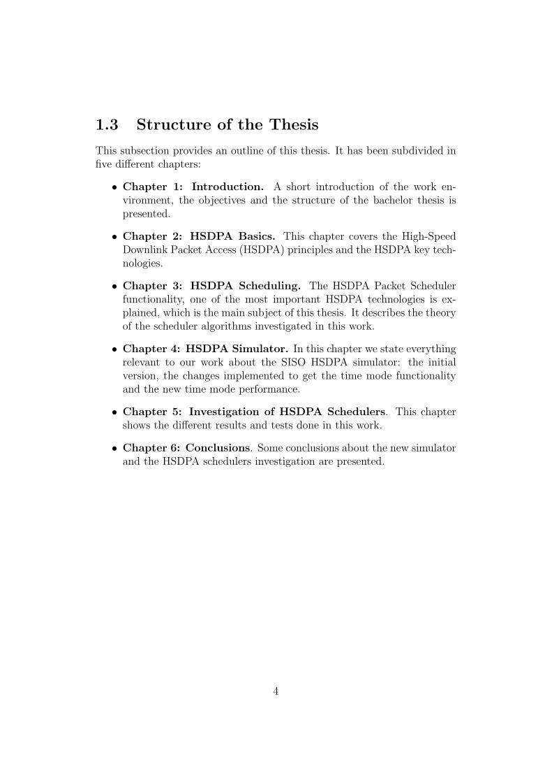
In HSDPA the transmission power is kept constant over the TTI (lengthof the frame is referred to as Transmit Time Interval) and uses AdaptiveModulation and Coding (AMC) as an alternative method to power controlin order to improve the spectral efficiency. HSDPA uses higher order modu-lation schemes like 16-Quadrature Amplitude Modulation (16QAM) besidesQPSK. The modulation to be used is adapted according to the radio channelconditions. QPSK can support 2 bits/symbol where as 16QAM can sup-port 4 bits/symbol, and hence twice the peak rate capability as comparedto QPSK, utilizing the channel bandwidth more efficiently. Different coderates used are 1/4, 1/2, 5/8, 3/4. The Node-B receives the Channel Qualityindicator (CQI) report and power measurements on the associated channels.Based on these information it determines the transmission data rate. In HS-DPA, users close to the Node-B are generally assigned higher modulationwith higher code rates (i.e. 16QAM and 3/4 code rate), and both decreasesas the distance between UE and Node-B increases. Figure 2.7 shows theend-user data-rate, not considering the overheads (i.e. CRC check, protocolheads).

14

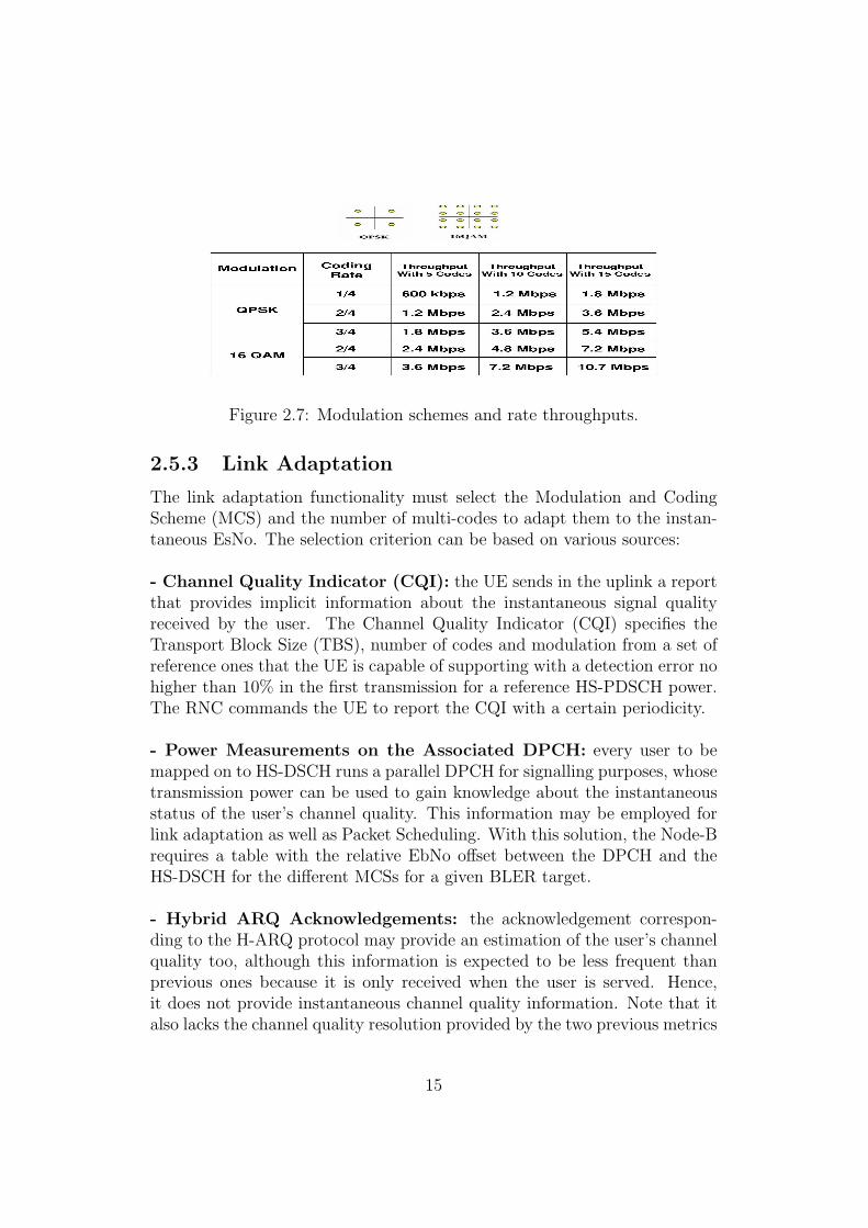
Figure 2.7: Modulation schemes and rate throughputs.

2.5.3 Link Adaptation

The link adaptation functionality must select the Modulation and CodingScheme (MCS) and the number of multi-codes to adapt them to the instan-taneous EsNo. The selection criterion can be based on various sources:

- Channel Quality Indicator (CQI): the UE sends in the uplink a reportthat provides implicit information about the instantaneous signal qualityreceived by the user. The Channel Quality Indicator (CQI) specifies theTransport Block Size (TBS), number of codes and modulation from a set ofreference ones that the UE is capable of supporting with a detection error nohigher than 10% in the first transmission for a reference HS-PDSCH power.The RNC commands the UE to report the CQI with a certain periodicity.

- Power Measurements on the Associated DPCH: every user to bemapped on to HS-DSCH runs a parallel DPCH for signalling purposes, whosetransmission power can be used to gain knowledge about the instantaneousstatus of the user’s channel quality. This information may be employed forlink adaptation as well as Packet Scheduling. With this solution, the Node-Brequires a table with the relative EbNo offset between the DPCH and theHS-DSCH for the different MCSs for a given BLER target.

- Hybrid ARQ Acknowledgements: the acknowledgement correspon-ding to the H-ARQ protocol may provide an estimation of the user’s channelquality too, although this information is expected to be less frequent thanprevious ones because it is only received when the user is served. Hence,it does not provide instantaneous channel quality information. Note that italso lacks the channel quality resolution provided by the two previous metrics

15

since a single information bit is reported.

- Buffer Size: the amount of data in the MAC-hs buffer could also beapplied in combination with previous information to select the transmissionparameters.

For an optimum implementation of the link adaptation functionality, proba-bly a combination of all the previous information sources would be need. Ifonly one of them is to be selected, the CQI report possibly appears as themost attractive solution due to its simplicity for the network, its accuracyand its frequent report, [11].

2.5.4 Fast Hybrid Automatic Repeat Request (H-ARQ)

In HSDPA a physical layer retransmission functionality is added that im-proves the HSDPA performance and gives robustness against link adapta-tion errors. Now that the HARQ functionality is located in the MAC-hsentity of the Node B, the transport block retransmission process is signifi-cantly faster than RLC layer retransmissions because the RNC or the Iubare not involved. This benefit is directly reflected on a lower UTRAN trans-fer delay, which has obvious improvements at end-to-end level (i.e. for TCP).

The retransmission protocol selected in HSDPA is the Stop And Wait (SAW)due to the simplicity of this form of ARQ. In SAW, the transmitter persists onthe transmission of the current transport block until it has been successfullyreceived before initiating the transmission of the next one. Since the continu-ous transmission to a certain UE should be possible, N SAW-ARQ processesmay be set for the UE in parallel, so that different processes transmit inseparate TTIs. The maximum number of processes for a single UE is 8. TheSAW protocol is based on an asynchronous downlink and synchronous uplink.

The Hybrid ARQ technique is totally different from the classical WCDMAretransmissions, because with HARQ the UE decoder combines the soft in-formation of multiple transmissions of a transport block at bit level. Notethat with this technique, the mobile terminal must store the soft informationof unsuccessfully decoded transmissions, so it requires some memory space.There exist different Hybrid ARQ strategies:

- Chase Combining: First proposed in [12]. It involves the retransmissionof the same data packet which was received with errors. Once the retrans-mission is received, the receiver combines the soft values of the original signal

16

and the retransmitted signal weighted by the SNR prior to decode the datapacket.

The advantages are: each transmission and retransmission can be decodedindividually (self-decodable), time diversity gain, and maybe path diversitygain. On the other hand, the disadvantage is that the retransmission of theentire packet is a wastage of bandwidth.

- Incremental Redundancy (IR): Incremental Redundancy is used toget an increased performance out of the available bandwidth. Here the re-transmitted block consists only of the correction data of the original data andcarries no actual information (Redundancy). The additional redundancy in-formation is sent incrementally when the first, second,. . . retransmissions arereceived with errors.

The advantage is that IR allows for a better decodability by decreasing theeffective coderate after combining the redundancy information. The disad-vantage is that the systematic bits are only sent in the first transmission andnot in the retransmission which makes the retransmissions non-self decod-able. So, if the first transmission is lost due to large fading effects there isno chance of recovering from this situation.

- Partial Incremental Redundancy: The partial IR is the combinationof chase combining and IR. The disadvantage with IR is removed here byadding the systematic bits along with the incremental redundant bits in theretransmissions. This makes both original and retransmitted signals selfde-codable.

2.5.5 Fast and Fair Scheduling at Node-B

Typically in WCDMA networks the packet scheduling is done at the RNC,but in HSDPA the packet scheduler is shifted to the Node-B, [10]. Thismakes the packet scheduling decisions almost instantaneous. In addition tothis, the TTI length is shortened to 2 ms. Figure 2.8 shows the schedulingscheme.

A first approach for fair scheduling can be the Round Robin method whereevery user is served in a sequential manner, so that all the users get thesame average allocation time. Another popular fair packet scheduling is pro-portional fair packet scheduling. A deeper analisys of the different HSDPAschedulers will be presented in Chapter 3.

17

Figure 2.8: Scheduling scheme.

2.5.6 Short Transmission Time Interval (TTI)

The length of the frame is referred to as Transmission Time Interval (TTI).The HS-DSCH which is added in the HSDPA standard uses a TTI length of2 ms compared to 10 ms TTI length in Release’99. This is done to reducethe round trip time, increases the granularity in the scheduling process andfor a better tracking of the time varying radio channel.

18

Chapter 3

HSDPA Scheduling

This bachelor thesis analyses the performance of the most common schedul-ing algorithms with different degrees of fairness among users. This chap-ter is organised as follows: Section 3.1 presents an introduction to HSDPAPacket Scheduling. In Section 3.2 we describe the different input informa-tion avalaible for the scheduler. Finally, Section 3.3 presents the schedulingalgorithms investigated in this bachelor thesis.

3.1 Introduction

As we have commented before, the Packet Scheduling functionality playsa key role in HSDPA. The features included in HSDPA and the new loca-tion of the scheduler in the Node-B open new possibilities for the designof this functionality for the evolution of WCDMA. The main goal of thePacket Scheduler is to maximize the network throughput while satisfying theQuality of Service (QoS) requirements of the users. In order to improve thecell throughput, the HSDPA scheduling algorithm can take advantage of theinstantaneous channel variations and temporarily raise the priority of thefavourable users. Since the users’ channel quality varies asynchronously, thetime-shared nature of HS-DSCH introduces a form of selection diversity withimportant benefits for the spectral efficiency, [11].

In UMTS, the bearers do not set any absolute quality guarantees (such cannever be given in a wireless transmission) in terms of data rate for interac-tive and background traffic classes. However the interactive users still expectthe message within a certain time, which could not be satisfied if any of

19

those users were denied access to the network resources. Because of that,the introduction of minimum service guarantees for users is a relevant fac-tor, and it is taken into consideration in the performance evaluation of thedifferent HSDPA schedulers. The service guarantees interact with the notionof fairness and the level of satisfaction among users. Very unfair schedulingmechanisms can lead to the starvation of the least favourable users in highlyloaded networks, and as described in [13], the starvation of users could havenegative effects on the performance of higher layer protocols, like TCP. Theseconcepts and their effect on the HSDPA performance are thus important forour investigation.

3.2 Parameters

The scheduler has diverse input information available, and we can classifythem in four different groups: resource allocation, UE feedback measure-ments, QoS related parameters and miscellaneous, [11].

3.2.1 Resource allocation

- HS-PDSCH and HS-SCCH Total Power: it indicates the maximumpower to be used for both HS-PDSCH and HS-SCCH channels. This amountof power is reserved by the RNC to HSDPA. Optionally, the Node-B mightalso add the unused amount of power (up to the maximum base station trans-mission power). Note that the HS-SCCH represents an overhead power (i.e.it is designated for signalling purposes), which could be non negligible whensignalling users with poor radio propagation conditions.

- HS-PDSCH codes: it specifies the number of spreading codes reservedby the RNC to be used for HS-PDSCH transmission.

- Maximum Number of HS-SCCHs: it identifies the maximum num-ber of HS-SCCH channels to be used in HSDPA. Note that having morethan one HS-SCCH enables the Packet Scheduler to code multiplex multipleusers in the same TTI, and thus increases the scheduling flexibility, thoughit also increases the overhead.

20

3.2.2 UE Channel Quality Measurements

the UE channel quality measurements aim at gaining knowledge about theuser’s supportable data rate on a TTI basis. All the methods employed forlink adaptation are equally valid for Packet Scheduling purposes (i.e. CQIreports, power measurements on the associated DPCH, or the Hybrid ARQacknowledgements).

3.2.3 QoS Parameters

Scheduling Priority Indicator (SPI): this parameter is set by the RNCwhen the flows are to be established or modified. It is used by the PacketScheduler to prioritise flows relative to other flows, [14].

Common Transport Channel Priority Indicator (CmCH-PI): thisindicator allows differentiating the relative priority of the MAC-d PDUs be-longing to the same flow, [15].

Discard Timer: is to be employed by the Node-B Packet Scheduler tolimit the maximum Node B queuing delay to be experienced any MAC-dPDU.

Guaranteed Bit Rate: it indicates the guaranteed number of bits persecond that the Node-B should deliver over the air interface provided thatthere is data to deliver, [14].

3.2.4 Miscellaneous

User’s Amount of Data Buffered in the Node-B: This information canbe of significant relevance for Packet Scheduling to exploit the multi-user di-versity and improve the user’s QoS.

UE Capabilities: They may be limiting factors like the maximum numberof HS-PDSCH codes to be supported by the terminal, the minimum periodbetween consecutive UE receptions, or the maximum number of soft channelbits the terminal is capable to store.

HARQ Manager: This entity signals the Packet Scheduler when a cer-

21

tain Hybrid ARQ retransmission is required.

3.3 Scheduling Algorithms

The operation task of the Packet Scheduler is to select the user to be servedin every TTI. Given the users in the cell we can define the desired operationof the Packet Scheduler as to maximize the cell throughput while satisfyingthe QoS attributes.

The Packet Scheduler distributes the radio resources among the users inthe cell. The scheduling algorithms that reach the highest system through-put tend to cause the starvation of the least favourable users (low G Factorusers), [16]. This behaviour interacts with the fairness in the allocation of thecell resources, which ultimately determine the degree of satisfaction amongthe users in the cell. For this reason, in each scheduler evaluation we considerboth parameters: fairness and sum cell throughput.

3.3.1 Maximum C/I

Scheduling strategies based on a C/I policy favour users with the best ra-dio channel conditions in the resource allocation process. This schedulingalgorithm serves in every TTI the user with largest instantaneous support-able data rate. This serving principle has obvious benefits in terms of cellthroughput, although it is at the cost of lacking throughput fairness becauseusers under worse average radio conditions are allocated lower amount ofradio resources. Nonetheless, since the fast fading dynamics have a largerrange than the average radio propagation conditions, users with poor averageradio conditions can still access the channel.

3.3.2 Round Robin

In this scheme, the users are served in a cyclic order. This algorithm allocatesequal resources to all users, regardless of their current channel conditions.This method outstands due to its simplicity, and ensures a fair resource dis-tribution among the users in the cell.

22

3.3.3 Proportional Fair Throughput

The goal of this kind of scheduling is to give all users the same averagethroughput, regardless of their radio channel quality. Note that this fairnessdefinition aims at the so-called max-min fairness. In [17] it is defined as”A set of user throughputs {i}, i=1,..,N is said to be max-min fair if it isfeasible (a set of user throughputs is said to be feasible if the sum of all theusers throughputs is lower or equal to the link capacity) and the through-put of each user λi can not be increased without maintaining feasibility anddecreasing λj for some other user j for which λj < λi ”. This implies thatusers under more favourable radio conditions get the same throughput asusers under less favourable conditions (i.e. users at the cell edge). This kindof scheduling can be seen as a form of inverse C/I scheduling, since userswith a low C/I must be allocated larger amount of resources in order to getthe same throughput. This scheduling method gives a fair user throughputdistribution at the cost of a lower cell throughput [18].

Scheduling Method Serve Order Radio Resources FairnessServing according Unfair Distribution

Maximum C/I to highest of radio resourceschannel quality in favour of high Ginstantaneous factor users

ProportionalRound Robin Round robin throughput fairness &

in cyclic order same amount of averageradio resources

Served according ProportionalProportional Fair to highest relative throughput fairness &

instantaneous same amount of averagechannel quality radio resources under

certain assumptions

Table 3.1: Summary of analysed scheduling methods

It is important to note that the notion of fairness does not give any informa-tion of the total amount of resources a user can obtain, but on the relativedistribution of resources among the users. This implies that, under the samedegree of fairness in the resource distribution (i.e. fair resources, like Round

23

Robin), the user may obtain different amount of absolute resources as thenumber of users in the system varies with the average load. However, theend user is only concerned about his absolute performance, and not abouthis relative performance compared to the rest of the users.

24

Chapter 4

HSDPA Simulator

This chapter contains all the information about the HSDPA simulator, whichwas used to develop this work. After the initial simulator has been explained,we will explain some changes that were necessary in order to get the func-tionality that allows us to include the packet scheduling functions in thesimulator. The chapter is organised as follows: Section 4.1 will explain theinitial HSDPA simulator created by M.Wrulich et al, [19]. Section 4.2 de-scribes how the new time-based simulator works, explaining all the small andbig changes done to achieve the neccessary new functionality.

4.1 Initial HSDPA Simulator

As we have commented before, in a collaboration of the institute of Com-munications and Radio-Frequency Engineering and Mobilkom Austria AG, aSISO HSDPA system-level simulator was developed. The simulator is devel-oped in MATLAB and allows for the simulation of a mixed traffic network,i.e. UMTS and HSDPA.

The first goal of this simulator was to measure the HSDPA performancein a mixed traffic network, because as we explained in the Chapter 2, one ofthe advantages of HSDPA is that it can be deplayed in an existing UMTSnetwork. The operation of HSDPA within an existing WCDMA network ispossible sharing the power amplifier and spreading codes.

In order to evaluate the network performance, the initial work investigatesthe average user throughput in a mixed carrier scenario (Release 4 DCH and

25

HSDPA) and deduce the optimum Node-B power split under different condi-tions by means of snapshot based network simulations. These results couldbe used by network operators for the cell operation planning, [19].

Now the initial SISO HSDPA simulator is going to be explained. As wecan see in the figure 4.1 we can divide the process in three different parts:set options, precalculations and simulation loop.

Figure 4.1: Three main parts in the simulator process.

4.1.1 Set Options

The first function called in the simulator is the one which load all the ne-cessary variables in the program, but before this step it is important to knowexactly what we want to simulate. Once we have decided what kind of net-work we are interested in, and what kind of results we want to observe, weassign the according settings.

The settings are divided in four groups: network, channel, user equipmentand simulator. With this intuitive division is easy to find and fix the valuesthat we want to use in the simulation. Figure 4.2 shows a graphical schemewith these groups and their subdivisions.

Network Settings

This part includes all the elements belonged to the network:

26

Figure 4.2: Main elements in a mobile radio communication and their re-spective groups of variables.

• R’99: this group contains the variables of the Release ’99 part, like thebandwith (5 MHz), the chiprate or the UMTS load in percent (respectthe total of the network).

• Node-B: in this part the distance between the Node-Bs is fixed, also itis assigned the power distribution of the Node-B and the power level ofeach Node-B: the maximum power, the CPICH power and the commonpower.

• Power distribution: determines the power distribution among theneighboring Node-Bs, thus specifying the intercell-interference struc-ture.

• HSDPA: in this part the number of users of the HSDPA simulation,the spreading factor of HSDPA transmissions (fixed at 16), the numberof codes, the absolute HSDPA power and the TTI value (usually 2 ms)are specified.

• MAC-hs: has not been used in the initial simulator, but it is the placefor the scheduling variables.

27

• Network structure: the number of base stations (7 or 19), the num-ber of sectors for each base station (1 or 3) and the model used for theantenna gain pattern can be chosen here.

• Other: here is the place for some variables like the grid density, whichdetermines the number of grid points for user positioning within thecell, or the G factor of the network.

Channel Settings

The channel settings are composed by the three fadings that influence thesignals in the communications between the base station and the users, andthe Power Delay Profile (PDP).

• Deterministic fading: once the model (COST231, Berger, fixed, ex-ponent, tr25848 or none) is selected, the neccesary variables to applyafter the functions are assigned.

• Shadow fading: in this initial version of the simulator it is only pos-sible to choose between the lognormal model or the lognormal movingmodel, loading their variables.

• Fast fading: here it is possible to select a simulation model for theRayleigh fading or choose not to include the fast fading.

• Power Delay Profile: the chiprate, the oversampling factor and themodel (pedestrian A or B, vehicular A or B) are specified.

User Equipment Settings

The groups included here define the general characteristics of the user equip-ments and some user specific things like the speed or the antenna type.

• General: includes the category class and the noise power seen by thereceiver.

• Movement: it will be used in the improved version developed in thisthesis.

• Receiver: selection of the receiver type and the number of fingers (incase of a Rake receiver).

• Traffic: will be used in further developements of the simulator.

28

Simulator Settings

The elements define in this part do not belong to the communication scheme,but determine some specific functions of the simulator.

• Simulation type: all the options are based on the snapshot scenario,but each type introduces a small variation in the simulation, i.e. ’ex-haustive snapshot’.

• Link performance model: the options are: ’COST290’, where asimple link performance model based on COST 290 is used, or ’none’,when no BLER (Block Error Rate) model is used (BLER = 0).

• R’99 datarate model: a simple data rate model described in [19].

• Power distribution: settings for the step-size of the power loop inthe simulator.

• Display/save results: backup options.

4.1.2 Precalculations

Once all the variables are loaded and we know the kind of simulation weare interested in, it is time to prepare the network before the simulationloop starts. The elements created in this step are: Node-B positions, userpositions, PDP for links in serving site, and the path losses for all the users.

Node-B positions

The Node-Bs position generation is implemented as an hexagonal networklayout, with the serving Node-B in the centre of the network, and then oneor two rings of concentrical Node-Bs around it (one ring if the total of BSs is7, and two rings if there are 19 BSs) this is the cell layout type 2 accordingto [20]. One example of the option with 7 Node-Bs is shown in Figure 4.3.

Users positions

The user position generation consists on two steps. First a grid of pointsinside the cell (the first sector of the serving node) is created, like Figure 4.4.After this process the users position is drawn randomly, with as many usersas we have decided in the settings that we want to simulate in the HSDPAtraffic simulation.

29

Figure 4.3: Layout with 7 base stations.

Figure 4.4: Example of the users’ grid generation in the serving cell.

Power Delay Profile (PDP)

In this part, the PDP for links in serving site, which is the same for all theusers, are generated. The PDP is different for each ITU model [21].

Users pathloss

This function generates the pathlosses from all Node-Bs in the simulated net-work structure to the given users. The radio propagation model used in thesimulator considers basically three different parts: deterministic pathloss d,shadow fading s, and small-scale fading with multiple paths and no correla-

30

Ped A Ped B Veh A Veh BDelay tap 1 (ns) 0 0 0 0

Coeff. tap 1 0.9923 0.6369 0.6964 0.3226

Delay tap 2 (ns) 110 200 310 300Coeff. tap 2 0.1034 0.5742 0.6207 0.5737

Delay tap 3 (ns) 190 800 710 8900Coeff. tap 3 0.0683 0.3623 0.2471 0.0301

Delay tap 4 (ns) - 1200 1090 12900Coeff. tap 4 - 0.2536 0.2202 0.0574



Table 4.1: PDPs of the different models.

tion in time, since this initial simulator is snapshot based with no correlationsin between, [19]. So the coefficient channel between the base station and theuser equipment can be written as:

h(τ) = d · s ·L∑t=1

√pl · fl · δ(τ − τl) (4.1)

where fl represents L independent Rayleigh fading proceesses at fixed timeslots, δ denotes the Dirac function and pl, τl are the relative power and delayof the multipath components.

The deterministic pathloss depends on the distance between the BS and theUE, which is modelled according to the COST231 model [22], and also de-pends on the antenna gain pattern if a sectorized model is used. The shadowfading is modelled by a lognormal random variable with zero mean and σs =8 dB, with no correlation in time.

4.1.3 Simulation Loop

Finally the system is prepared to start the simulation of multiple independentsnapshots, getting the results after the average of these individual calcula-

31

tions. The first two parts have the simulator with all the network created andall the values loaded, Figure 4.6 illustrates the BS and the user distribution,using 19 Node-Bs and a 3 sectors model. It is important to note that all thesimulations are done in the first sector (with the main radiation in 90o) ofthe serving Node-B, and is furthermore called the ”target sector”.

Figure 4.5: Network with 19 base stations and 3 sectors model.

Before starting the detailed explanation of the way of modeling the HS-DPA and R’99 traffic, it is necessary to talk about the power split betweenboth transmission types, and also to discuss the two different possibilities ofallocating the power of HSDPA in the base station downlink power budget.

Power split

The total available transmit power in each cell is shared between HSDPAand DCH users. The expression of the total intracell transmission power is:

Pintra = PDCH + PHS−DSCH + Pother (4.2)

32

where Pother incorporates the power from other needed channels, like thecommon pilot channel (CPICH) or the common channel. In the simulator,the total power, the R’99 load in percent respect this total power and thedifferent powers included in the Pother are set in the first part, and accord-ingly the HSDPA power range is determined.

About the possibilities of allocating the power of HSDPA, there are twooptions of which both are implemented in the simulator:

• The RNC can dynamically allocate HSDPA power by sending Node-Bapplication part (NBAP) messages to the base station, which effectivelykeeps the HSDPA power at a fixed level, whereas the DCH power variesaccording to the fast closed loop power control.

• The second option is when no NBAP messages are sent and the basestation is allowed to allocate all unused power for HSDPA, which betterutilises the power amplifier, [19].

HSDPA System Level Modelling

In principle, a network simulation could be performed by means of an blown-up link-level simulation (incorporating the full physical layer, e.g. channelcoding, inter leaving, etc.), but this would result in an unfeasible computa-tional complexity. So, it was neccessary to derice a simplified system leveldescription to model the individual links, avoiding the complexity but havingstill an accurate representation of the HSDPA performance, [19].

The first step is to evaluate the channel quality as observed by the receiver,this part is called link-measurement model, where it was assumed that astandard single antenna Rake receiver is used because it is the most com-mon in the SISO HSDPA terminals. The metric used for this evaluation isthe signal-to-noise-and-interference ratio (SINR), it is calculated after Rake-combining and despreading for each user u in the cell, according to

SINRu =

NF∑i=1

SF · PHS−DSCHγ

· |hi|2

Pintra,residual + Pinter + Pnoise(4.3)

33

where SF is the spreading factor, PHS−DSCH is the power used for the HS-DSCH, γ represents the number of assigned spreading codes, Pintra,residual isthe residual intracell interference in the downlink, Pinter is the transmittedinterfering power from the neighbouring base stations, and Pnoise is the noisepower as seen at the receiver. The residual intracell interference is given by[23], Pintra,residual = Pintra ·

∑Ll=1 |hl|2, where L denotes the total number of

taps of the current realisation, denoted by hl, and Pintra is the total powertransmitted in the serving cell, [19].

In the simulator, the transmission power of the HS-DSCH is divided equallybetween all used HS-PDSCH. In Equation (4.3) structure of the Rake re-ceiver is implicitly shown, where in the numerator the useful power is addedup, which is cancelled out from the interference power in the denominator.This is consecutively done for all the NF available fingers. In addition, itwas assumed that perfect channel state information (CSI) is available at thereceiver so that the receiver weights and the location of the fingers can bechosen perfectly. Considering that, only the squared absolute values of thechannel coefficients (for each tap), |hi|2 appear in the equation.

Once the SINR is determined, the simulator calls the function to computethe quantized CQI value for a given SINR, using the expression described in[24]:

CQI = SINR[dB] + 3.5. (4.4)

Each CQI value represents a specific combination of the number of codes,modulation type and transport block size; and is used by the link adaptationalgorithm at Node-B. The range of values of the CQI index is 0 to 30, whereeach value indicates the maximum TBS that can be correctly received with90% probability (as mentioned before).

After the channel quality is evaluated, the second part consists on describingthe bit-error/decoding performance, also called link-performance model. Ananalytical approach based on link-level simulations was selected, as in [24].In the simulator a link performance modelling for the transport formats ofeach mobile category class is utilized, given by the range of possible CQIvalues. The tables for each category, used to determine the Transport BlockSize (TBS), the number of codes as a function of the CQI, and specifying

34

Figure 4.6: SINR to CQI mapping.

the number of spreading codes, are implemented from [25]. One example ofthese tables is shown in Table 4.1, valid for the UE categories 1 to 6, whichhas been used during the HSDPA schedulers investigation.

The Block Error Ratio (BLER) is calculated according to an analyticalmodel, as specified in [24]. The BLER, under AWGN conditions and utilizinga standard Rake receiver together with turbo coding, can analitically be wellapproximated by Equation (4.5), as in [26]. The BLER is considered directlyin the evaluation of the throughput.

BLER = [102SINR−1.03CQI+5.26√

3−log10(CQI) + 1]−10.7 (4.5)

The TBS denotes the maximum amount of data that can be transmittedvia the network in one TTI of 2 ms to the UE without exceeding a BLERof 0.1 in average. Accordingly the HSDPA user data rate is calculated as inthe Equation (4.6), which is consecutively averaged over fading realizations,and finally averaged over all the individual snapshot simulations to get the

35

CQI value Transport Block Size Nr of HS-PDSCH Modulation0 N/A QPSK1 137 1 QPSK2 173 1 QPSK3 233 1 QPSK4 317 1 QPSK5 377 1 QPSK6 461 1 QPSK7 650 2 QPSK8 792 2 QPSK9 931 2 QPSK10 1262 3 QPSK11 1483 3 QPSK12 1742 3 QPSK13 2279 4 QPSK14 2583 4 QPSK15 3319 5 QPSK16 3565 5 16QAM17 4189 5 16QAM18 4664 5 16QAM19 5287 5 16QAM20 5887 5 16QAM21 6554 5 16QAM22 7168 5 16QAM23 7168 5 16QAM24 7168 5 16QAM25 7168 5 16QAM26 7168 5 16QAM27 7168 5 16QAM28 7168 5 16QAM29 7168 5 16QAM30 7168 5 16QAM

Table 4.2: CQI mapping table for UE categories 1 to 6, from [25].

HSDPA data rate.

Ru = TBS · 1

2ms· (1−BLER). (4.6)

36

The simulator applies the case that the user always get the full availablepower, and there is enough data to transmit (full buffer assumption). It isimportant to note that in the snapshot based simulation approach, no HARQretransmissions are modelled.

Finally, an overview of the described HSDPA calculations are illustratedin Figure 4.8, where we can observe the SINR evaluation as the first step.After that, the CQI is mapped as function of the SINR, and using both, theBlock Error Rate (BLER) and the Transport Block Size (TBS) we are ableto estimate the HSDPA data rate.

Figure 4.7: Overview of the HSDPA calculation

R’99

As we have commented before, the main objective of the initial investigationwas the prediction of the achievable HSDPA user data rates in dependence ofa given Release 4 DCH load in the cell. So, the Release 4 traffic is mo-delledonly coarse, the simulator just needs to roughly estimate the total DCH cellthroughput in order to be able to predict the overall cell throughput, [19].

37

The R’99 data rate evaluation use a link quality equation for DCH down-link connections proposed by [27], and also assumes the same kind of servicefor all DCH users in the cell. With these assumptions, an analytical modelcould be derived to predict the average R’99 cell throughput as function ofthe power distribution, [19].

4.1.4 Results

In order to have a better idea about the first objectives of the HSDPAsi-mulator, we shortly present one of the main optimizations evaluated byM.Wrulich using the initial version of the simulator, which has been ex-plained in this section. It is an investigation to identify the optimum powersetting to maximize the total cell throughput, in the case of the RNC con-trolling the HS-DSCH power.

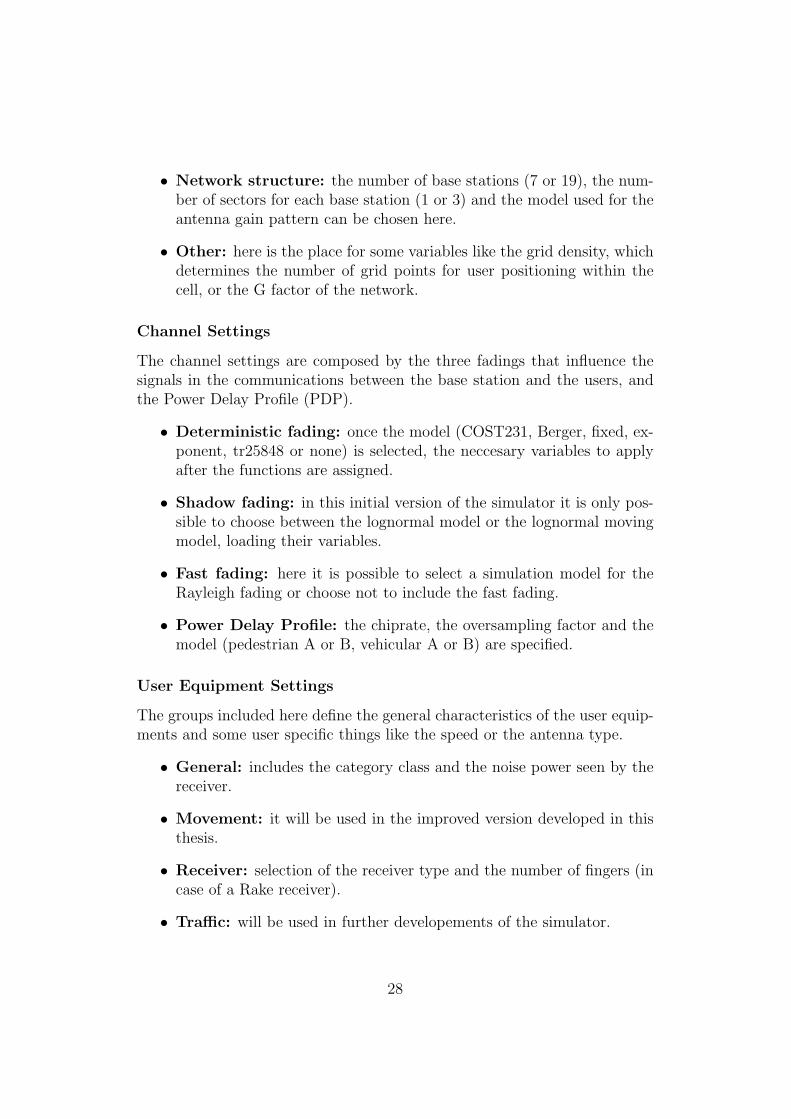
With the simulator the evolution of the total cell data rate, the HSDPAuser data rate and R’99 cell data rate, in dependence of the power assignedto the HS-DSCH can be analysed. The result of the simulation is shown inFigure (4.9), with a Release 4 load of 20%, and a Node-B distance of 0.5km, Pedestrian A model, 10 codes used for HS-DSCH and the users utilizedequipments of capability class 6. In the figure we can see the maximum to-tal cell data rate when the power assigned to HS-DSCH is 4.605 W, and themaximum HSDPA user data rate in PHS−DSCH = 6.029 W. The HSDPA userdata rate does not grow unlimited because an increase in power also increasesthe intercell interference. On the other hand, the R’99 cell data rate dropsdown since the start, because of the monotounuesly increasing interferenceseen by these transmissions.

4.2 New HSDPA Simulator: Continuos Time

Simulation

In this section the simulator used for the scheduler investigation is described.Firstly, an overview to the new mode and the changes in the code structurewill be presented. Then, we will begin the individual and detailed explanationof the main parts changed in the simulator, starting with the multipath andshadow fading, including the simulation model we use and the MATLABfunctions implemented (as a small part of code example). After that we will

38

Figure 4.8: Average data rates with RNC power control of the HS-DSCH.

discuss the users movement, because in a simulation over time, we have amore realistic network simulation with the users moving inside the cell. Inaddition, we will show the new SNR to CQI mapping used in the new versionof the simulator. Subsection 4.2.6 explains the implementation of the threeHSDPA schedulers evaluated in this work.

4.2.1 Time Mode Simulator

The simulator transformation forced us to make continuos modifications inthe code structure. The first thing that we have to comment is that becauseof the multiple changes, the code was divided into two groups separated byfunctionality. When the options are set, there are some common parame-ters and also some specific parameters for each mode, which are loaded independence of the selected mode. The time based simulator has also newvariables, like the ones which determine the users movement (i.e. angle) orthe ones about the schedulers (i.e. type, number of users scheduled). Alsoit is relevant to note that in the time mode the concept of number of sim-ulation runs has dissapeared in favour of the concept of simulating over time.

39

In the precalculation part, the Node-Bs and users position generation isbasically like in the initial version, and also the creation of the PDPs islike before. However important changes were necessary in the user pathlossgeneration. Now that the users are moving inside the cell, we cannot pre-calculate the deterministic pathloss because for every slot the user positionwill be different, and consequently the deterministic pathloss (macrocospicpathloss) suffered by the users will be different for each time slot too.

So, in the precalculations of the time-based simulator, we are only able togenerate the non-deterministic pathloss that consists of the multipath andshadow fading. In spite of a big number of uncorrelated values to simulate themultipath and shadow fading (the number depended on the nr. of simulationruns), it was neccessary to find a good model to generate the correlated fad-ing over time of both fadings. For each user as many multipath and shadowtraces as sectors exists are generated (i.e. with 19 BSs and 3 sectors model,each user has 57 different traces). In Subsections 4.2.2 and 4.2.3, both areexplained in greater detail.

Let us now discuss the main simulation loop. First, it is fundamental tonote that now the loop is over time, and the total time simulated is set usingthe number of time slots (i.e. 30.000 slots = 10.000 TTI = 20 seconds). Atthe beginning of the loop, the first thing calculated is the new users position(after one slot has passed) and then it is checked if all the users are stillinside the cell (the users movement is widely described in Subsection 4.2.4).After that, we are ready to calculate the deterministic pathloss for each user(based on the distance and angle between the user and the transmitting sec-tors) and the total pathloss, by evaluating the macro-scale (deterministic)pathloss, the shadow fading and the multipath fading.

After these user dedicated evaluations, the simulator starts to calculatebasically the same metrics as in the original simulator. However, some im-portant changes were necessary to let the simulator handle the time-domain.

As we have commented before the loop is over time slots, but transmis-sions occur every TTI (1 TTI = 3 slots). Thus, we calculate the users SINRin every slot and after three time slots have passed (see Figure 4.11), webegin with the HSDPA dedicated evaluation. The first thing calculated isthe average SINR over the last three slots. Once we know this SINR, thenext step is to map the CQI as function of the SINR, but with a differentequation respect to the initial version (the new functionality is explained inSubsection 4.2.5). It has to be noted that, because of the delay of the feed-back information, the simulation works with the CQI obtained some TTIs

40

Figure 4.9: Flow Diagram of the new time mode.

before. The delay of the feedback information is set in the options of thesimulator.

Figure 4.10: New SINR calculation.

In the HSDPA calculation, we simulate the network in each TTI consid-ering the current SINR (averaged over the last 3 slots) and a previous CQI.After the SINR information is known, the scheduling function is introducedin the simulation. Depending on the selected scheduler a different algorithmis used. Using the scheduler algorithms the served users in the current TTI

41

are choosen. The three different tested schedulers are described with detailin Subsection 4.2.6 .

Now that the scheduled users are known, the remaining steps of the HS-DPA throughput evaluation can be executed. For each served user, first theTBS and the necessary number of spreading codes are obtained, followingthe tables specified by 3GPP. These tables are specified according to the UEcategory. Second, the BLER is estimated as in the initial version of the simu-lator (see Equation (4.5)), based on the CQI and the SINR of the user. Usingboth parameters (TBS and BLER) the amount of data transmitted to eachserved user is calculated. The BLER is used as a probability to determineif the transmission has been decoded correctly or not. In the positive case,the data transmitted to the user is equal to the TBS, in the opposite casehowever, the amount of transmitted data equals zero.

Figure 4.11: New HSDPA throughput evaluation scheme

So, for each user, we sum up all the transmitted data, and when the simula-tion has finished, the respective HSDPA user data rates are known. All theresults concerning the time-based simulator will be shown in Chapter 5. Letus now go into more detail and discuss the parts of the simulator mentionedabove.

42

4.2.2 Multipath Fading

Let us now provide a complete description of the multipath fading. We willstart with a short definition, and explain the mathematical model and thesimulation model afterwards. Finally we show the MATLAB implementedfunction and one example trace.

Definition

Multipath propagation is a phenomenon that affects all wireless systems.Multipath fa-ding is created when radio waves, arrive at a receiving antennafrom different paths, of course, the superposition of the incoming waves canbe constructive or non-constructive. Multipath fading occurs irrespective ofradio signal strength and is particularly common in urban areas where radiowaves do not have a line of sight path between the transmitter and the re-ceiver. Causes of multipath include atmospheric ducting, ionospheric reflec-tion and refraction, and reflection from terrestrial objects, such as mountainsand buildings. The figure 4.13 illustrates a simple scheme of the multipathcauses.

Figure 4.12: Scheme with the multipath causes

Multipath fading may be minimized by diversity techniques, e.g. space andfrequency diversity. In space diversity, two or more receiving antennas arespaced some distance apart. Fading does likely not occur simultaneously atboth antennas. Therefore, enough output is almost always available from oneof the antennas to provide a useful signal. In frequency diversity, two trans-mitters and two receivers are used, each pair tuned to a different frequency,

43

with the same information being transmitted simultaneously over both fre-quencies. One of the two receivers will almost always produce a useful signal.

Multipath fading can be statistically described by a Rayleigh fading [28].In digital radio communications multipath can cause errors due to ISI andthus affect the quality of communications. Techniques to combat this aree.g. OFDM, Rake receivers or equalizers.

Simulation Model for Rayleigh Fading Channels

About the last three decades, the well-known mathematical reference modeldue to Clarke [29] and its simplified simulation model due to Jakes [30] havebeen widely used for Rayleigh fading channels. But in the multiple uncor-related fading waveforms generation for frequency-selective fading channelsand multiple-input multiple-output (MIMO) channels, the Jakes’ simulatorhas problems, because it is a deterministic model. Therefore, different mod-ifications of Jakes’ simulator have been reported in the literature (i.e. [31],[32], [33]).

In this work, we present the statistical simulation for Rayleigh fading chan-nels proposed in [1], whereas we implemented this model with a variationintroduced by Zemen in [34]. This simulator can be directly used to gen-erate multiple uncorrelated fading waveforms for frequency selective fadingchannels, MIMO channels, and diversity combining scenarios. The variationintroduced by Zemen is for time-variant channels with Jakes’ spectrum es-pecially for low speeds.

In the simulator proposed in [35] random phase shifts are introduced toremove the stationarity problem. But with this improvement other troublesappeared, because higher-order statistics may not match the desired ones,as proven in [36]. In addition, even if the number of sinusoids approachesinfinity the results are not matching, [30]. In [1] a new sum-of-sinusoids sta-tistical simulation was proposed, which solves the problem of the high-orderstatistics, and also achieves good approximations even when the numberof sinusoids is as small as eight and the number of random trials is only50. For us, this model is useful because it can be directly used to gener-ate multiple uncorrelated fading waveforms, which are needed to simulaterealistic frequency-selective fading channels, MIMO channels, and diversity-combining scenarios.

Based on the Jakes’ simulator family, but considering the modified model

44

proposed by Pop and Beaulieu in [35], the improvement of the simulationmodel explained is based on reintroducing the randomness for all three ran-dom variables Cn, αn, and φn. It consideres the following simulation proto-type function to introduce the randomness in these variables:

g(t) = E0

N∑n=1

Cnexp{j(wdtcos(αn) + φn)} (4.7)

where

Cn =exp(jψn)√

N, n = 1, 2, ..., N (4.8)

αn =2πn− π + θ

N, n = 1, 2, ..., N (4.9)

φn = −φN2

+ n= φ, n = 1, 2, ..., N/2 (4.10)

with N/2 being an integer, and ψn,θ, and φ being mutually independent ran-dom variables uniformly distributed on [-π,π). The reintroduced randomnessin these variables enables to establish a new statistical and widesense sta-tionary (WSS) simulation model for Rayleigh fading channels. By choosingψN/2+n = ψn, gives the possibility to rearrange Equation (4.7) as:

g(t) =E0√N{N/2∑n=1

ejψn [ej(wdtcos(αn)+φ + e−j(wdtcos(αn)+φ]}. (4.11)

The first expression in the sum represents waves with radian Doppler fre-quencies that progress from the range of [wdcos(2π/N),wd] to the rangeof [-wdcos(2π/N),-wd], while the radian Doppler frequencies in the secondterm of the sums shift from the range of [-wdcos(2π/N),-wd] to the rangeof [wdcos(2π/N),wd]. Therefore, the Doppler frequencies in these terms areoverlapping. To represents the fading signals whose Doppler frequencies donot overlap, it is possible to simplify g(t) as:

g(t) =E0√N{M∑n=1

√2ejψn [ej(wnt+φ + e−j(wnt+φ]} (4.12)

45

where M = N/4, and wn = wdcos(αn). The factor√

2 is included to makethe total power remain unchanged. Based on Equation (4.12), the normal-ized low-pass fading proccess of a new statistical sum-of-sinusoids simulationmodel is defined by:

X(t) = Xc(t) + jXs(t) (4.13)

Xc(t) =2√M

M∑n=1

cos(ψn). cos(wdtcosαn + φ) (4.14)

Xs(t) =2√M

M∑n=1

sin(ψn). cos(wdtcosαn + φ) (4.15)

with

αn =2πn− π + φ

4M, n = 1, 2, . . . ,M (4.16)

where θ, φ, and ψn are statistically independent and uniformly distributedover[-π,π) for all n.

With this model the second-order correlation statistics match the desiredones exactly, even if the number of sinusoids is small; fourth-order statisticsasymptoticall match the correct ones as the number of sinusoids approachesinfinity. And as we have indicated before, with this simulation model it isdirectly possible to generate multiple uncorrelated fading waveforms.

Simulation Model

Finally we implemented in the HSDPA simulator the same simulation modelfor time-variant channels with Jakes’ Spectrum as proposed in [34]. Thismodel is based on the model from [1] with a correction for low velocitiesbased on [37]. This model ensures a Rayleigh distribution of h[m] for allvelocities v and even at v = 0 m/s.

The detailed simulation model for h[m] is given by:

h[m] =1√2

(hc[m] + jhs[m]), (4.17)

46

hc[m] =2√A

A∑i=1

cos(ψi) · cos(2πvDm cosαi + φi), (4.18)

hs[m] =2√A

A∑i=1

sin(ψi) · cos(2πvDm cosαi + φi), (4.19)

with

αi =2πi− π + φ

4Afor i ∈ {1, . . . , A}, (4.20)

where θ, θi, and ψi are independent and uniformly distributed over [-π,π)for all i . For our investigations, we usually fix the number of interferingpaths to A = 50.

MATLAB code

function [fading time] = xf jakes(nr slots,nr paths,V,TTI,F)

% function to generate Rayleigh fading with Jakes model% input: nr slots ... nr. of realizations% nr paths ... nr. of interfering paths% V ... velocitie of the UE% TTI ... Transmission Timing Interval% F ... frequency (in MHz)% output: fading time ... vector fading realizations

%% Functionality

% slot time (TTI/3)t slot=TTI*1e-3/3;% Doppler Frequency (V*F/Co)Vd=(V/3.6)/3e8*F*1e6;m=1:nr slots;k=2*pi*Vd*t slot;

47

% independent and uniformly over [-pi,pi)phi=2*pi*rand(nr paths,1)-pi;psi=2*pi*rand(nr paths,1)-pi;alpha=((2*pi*[1:nr paths])-pi+phi(1,1))/(4*nr paths);

h c=zeros(1,nr slots);h s=zeros(1,nr slots);

for i=1:nr paths

aux=cos(k*m*cos(alpha(i))+phi(i));h c=h c+cos(psi(i))*aux;h s=h s+sin(psi(i))*aux;

end

fading time=sqrt(2/nr paths)*(h c + j*h s)’;

end

The figure below shows an example of the MATLAB function that we createdto simulate the Rayleigh fading with the follow settings: nr. slots = 3000,nr. paths = 50, Vel = 3km/h, TTI = 2ms and Freq = 2000MHz.

4.2.3 Shadow Fading

Definition and simulation models

Shadowing is the reduction in signal strength occuring as a result of the UEsmoving in and out of the shadows of large obstacles such as buildings. Wepresent the two different kind of models used in our simulator to generatethe shadow fading: an uncorrelated model (used for snapshot simulations)and a correlated model (used for time-based simulations).

Uncorrelated Model In this case the shadow fading effect is usuallymodeled by a log-normal random variable, with the mean m usually given by0 dB, and the standard deviation σ depending on the propagation environ-ment (i.e. 8 dB for urban areas). This random variable is Gauss distributed

48

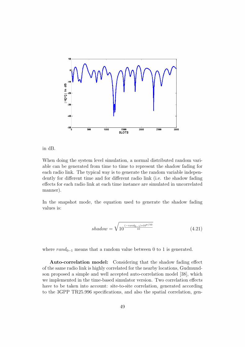
in dB.

When doing the system level simulation, a normal distributed random vari-able can be generated from time to time to represent the shadow fading foreach radio link. The typical way is to generate the random variable indepen-dently for different time and for different radio link (i.e. the shadow fadingeffects for each radio link at each time instance are simulated in uncorrelatedmanner).

In the snapshot mode, the equation used to generate the shadow fadingvalues is:

shadow =

√10

(−rand0−1)∗10σ/10

10 (4.21)

where rand0−1 means that a random value between 0 to 1 is generated.

Auto-correlation model: Considering that the shadow fading effectof the same radio link is highly correlated for the nearby locations, Gudmund-son proposed a simple and well accepted auto-correlation model [38], whichwe implemented in the time-based simulator version. Two correlation effectshave to be taken into account: site-to-site correlation, generated accordingto the 3GPP TR25.996 specifications, and also the spatial correlation, gen-

49

erated according to Gudmundson.

Gudmundson recommends an auto-correlation of

Figure 4.13: Scheme of the shadow fading

Rs(k) = S2a|k| (4.22)

a = εvTs/DD (4.23)

for the shadow faing, where a is the correlation coefficient, σ is the stan-dard deviation, εD is the correlation between two locations separated bydistance D, v is the mobile velocitie and Ts is the sampling interval.

MATLAB code

function [shadowfading] = xf shadowfading gudmundson(shadow,intersite constant)

% function to generate spatially (eq. temporally for constant speed) shadow% fading according to the model proposed by Gudmundson% (”correlation model for shadow fading in mobile radio systems”)% input: shadow ... structure of shadow settings% output: shadowfading ... trace of correlated shadow fading coefficients% (in dB)

50

% two correlation effects have to be taken into account% - site-to-site correlation (generated according to 3GPP TR25.996)% - spatial correlation (generated according to Gudmundson)

% white Gaussian random process, var=1tmp gauss = randn(shadow.nr samples,1);

% autocorrelation of desired fadingfilter coeff = shadow.corr coeff(shadow.vkmh/3.6*shadow.t samp/. . .shadow.corr distance);

% gauss with desired autocorrelationtmp s = filter(1,[1,-filter coeff],tmp gauss);% normalizetmp s = tmp s*sqrt(1-filter coeff2);% scale by given shadow fading variancetmp s = shadow.std*tmp s;

% correlated shadow fading (linear scale)shadowfading = exp((sqrt(1-shadow.site2site corr)*tmp s + . . .sqrt(shadow.site2site corr)*intersite constant)/10);

end

The figure below shows an example of the MATLAB function that we cre-ated to simulate the shadow fading, following the Gudmundson model. Thisexample generated by defining these values: nr. slots = 3000, correlationcoefficient a = 0.3, correlation distance εD= 55 m, v = 3km/h, TTI = 2msand σ = 8 dB.

4.2.4 Users Movement

Now that the users are simulated continuously in time, it was neccessaryto implement the movement of the users within the cell. Accordingly, themacro-scale pathloss and the antenna gain change with the position of theuser. Furthermore, the statistics of the shadow fading and the multipathfading depend on the user speed.

To model the users movement we decided to create two new variables as-

51

signed to the users: angle (randomly between 0-360 degrees) and speed.With these variables and the position of the user, we are able to calculatethe user position in the next time slot. Our simulation bases on the assump-tion that the number of simulated users in the cell stays constant, thus wehad to catch the case when a user moved out of the cell. The possible optionswere the following:

• Users rebouncing inside the cell. When the user reaches the limitof the cell, it rebounces to another direction inside the cell. Is easyto see that selecting this option the cell always have the same numberof users. An example of this way of implementation, using four users,would be like in Figure 4.14.

• User out, new user in. When the user leaves the cell, a new useris generated inside the cell, with the position being drawn from a uni-form distribution within the cell. The new user has their own angle ofmovement and starts their own simulation. Of course with this optionwe achieve again the same number of users in the cell during the wholesimulation.

In this work, we decided in favour of the second option. So each time slotwe check if the user has left the cell or not, and in case he did, we generatea new user in the place of the previous one, assigning an initial position anda new angle of movement. An example of the resulting users movement isdepicted in Figure 4.15.

52

Figure 4.14: User rebounding inside the cell

Figure 4.15: User out, new user in

The initial users position assigment is like in the first version of the sim-ulator (uniformly and randomly over the first sector of the serving node).But in the time-based simulator, a low number of HSDPA users are set (i.e.15). In the snapshot based simulator a high number of HSDPA users wereused (i.e. 500) trying to cover a big part of the cell in order to avoid thepossible bad results of the random users position and get an accurate esti-

53

mation of the cell throughput.

On the other hand, in the time mode simulations we use only around 15users, because of two main reasons: now that the users are moving insidethe cell, the positions change and we are well protected against the possiblenegative random effects having a realistic situation where we don’t need tocover the cell with hundreds of users, and secondly, we have to control thepotential MATLAB problems with memory and a more complex code.

4.2.5 New SNR to CQI Mapping

As we have already said, the Channel Quality Indicator is the indicator forHSDPA downlink channel quality. UE reports CQI and HARQ-ACK feed-back information to Node-B through uplink channel HS-DPCCH. The rangeof CQI values is 0-30, and each step corresponds appoximately to a 1 dB stepin HS-DSCH SINR. By means of the CQI, the maximum TBS that can bereceived correctly with at least 90% probability is indicated.

In the new simulation mode we opted for the Equation (4.24), which is alsoused in many of our consulted papers and articles, like in [26] or [39].

CQI =

0 if SNR ≤ -16,

bSNR1.02

+ 16.62c if -16 ≤ SNR ≤ 14,

30 if 14 ≤ SNR

(4.24)

now this is the formula used to compute the CQI from the measured valueof SNR.

4.2.6 Schedulers

Here we will describe how to simulate each scheduler (including the parame-ters it needs and the specific keys of the implementation). Let us begin withthe explaining how the HSDPA power and the codes are shared between theserved users.

In the snapshot mode, it is supossed that the total HSDPA power and themaximum number of codes are available to each user. This distribution ispossible because we evaluate the HSDPA network calculating first the indi-vidual user throughput and then the average over all the users. But now, due

54

to the possibility of multi-code scheduling it is necessary to split the powerand the number of codes equally among the users. Then, once the numberof served users is selected, the power and codes are divided by this number.Here we can see a simple example:

PHSDPA = 12 WNr. of codes = 15

Nr. of served users = 3

Puser = 4 W with 5 codes per user.

Obviously, if one user is scheduled, it will have all the power and all thecodes available. Before we took the decision of an equal distribution amongthe users, many of the 3GGP related specifications and papers were widelystudied, trying to verify that we don’t break the requirements. In futureenhancements of the simulator, it would be interesting to investigate othercombinations in the power and the nr. of codes distributions, in order toimprove the network performance in terms of throughput or QoS.

Figure 4.16: Example with the power and codes split when serving multipleusers

Maximum C/I

As we explained in Chapter 3, the scheduling strategies based on a C/I policyfavours users with the best radio channel conditions in the resource allocation

55

process. The maximum C/I serves in every TTI the user with largest instan-taneous supportable data rate (in the simulator, the CQI is the paremeterused to determine the transport block size). This serving principle has obvi-ous benefits in terms of cell throughput, although it is at the cost of lackingthroughput fairness.

The implementation of this scheduler was simple, it consists of elaborat-ing the priority table of the users, utilizing the reported CQI values. Thetable is arranged from the higher to the lower CQI, so the first n users inthis table are the ones selected to be served.

Figure 4.17 shows an example with the user position, the CQI that the usershave in this moment, and also the users to be served (after the delay) de-pending on the number of scheduled users.

Figure 4.17: Example of the maximum C/I scheduler decisions.

Round Robin

In this algorithm the users are served in a cyclic order. The round robinscheduler allocates equal resources to all users, regardless of their currentchannel conditions. This method outstands due to its simplicity, and ensuresa fair resource distribution among the users in the cell.

56

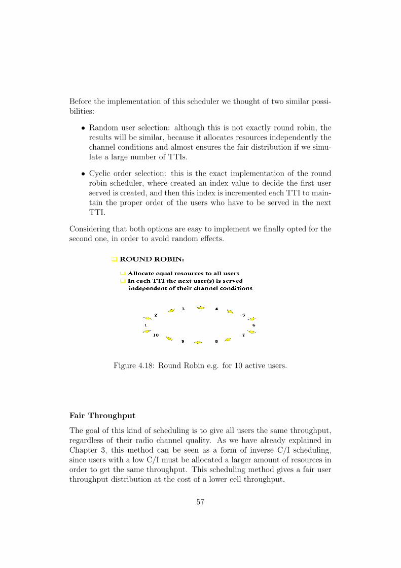
Before the implementation of this scheduler we thought of two similar possi-bilities:

• Random user selection: although this is not exactly round robin, theresults will be similar, because it allocates resources independently thechannel conditions and almost ensures the fair distribution if we simu-late a large number of TTIs.

• Cyclic order selection: this is the exact implementation of the roundrobin scheduler, where created an index value to decide the first userserved is created, and then this index is incremented each TTI to main-tain the proper order of the users who have to be served in the nextTTI.

Considering that both options are easy to implement we finally opted for thesecond one, in order to avoid random effects.

Figure 4.18: Round Robin e.g. for 10 active users.

Fair Throughput

The goal of this kind of scheduling is to give all users the same throughput,regardless of their radio channel quality. As we have already explained inChapter 3, this method can be seen as a form of inverse C/I scheduling,since users with a low C/I must be allocated a larger amount of resources inorder to get the same throughput. This scheduling method gives a fair userthroughput distribution at the cost of a lower cell throughput.

57

The concept of proportional fairness was introduced in [40] in the setupof a shared resources allocation problem in a generalised network, and thisconcept can also be adapted to HSDPA based wireless networks. There aremany authors who propose fair schedulers, but each one introducing someparticular variations to simulate it. We analysed some papers, like [39], [41],[42], [43], [44] and [45]. Finally we decided to implement in our simulatorthe proportional fair scheduling algorithm proposed in [39].

In [39] is indicated that a set of throughputs ri is proportionally fair if itis feasible (i.e. ri > 0 and

∑ni=1 ri < C ) and for any other feasible vector r∗i ,

the sum of the poroportional changes is 0 or negative, i.e.

n∑i=1

r∗i − riri

≤ 0. (4.25)

The proportional fair algorithm, as originally proposed in [46], selects user jby:

j = arg max1≤i≤nri(k)

rei(k). (4.26)

The average throughput is obtained by the following exponential weightedmoving average of the instantaneous data rate ri:

rei(k) =

{(1− α)rei(k) + αri(k) if i served in slot k,

(1− α)rei(k) otherwise,(4.27)

where 0 < α < 1 is a weighting factor, whose value may be chosen e.g.as 0.001, [46]. It has to be noted that by α→ 0, Equation (4.26) will provideequal air time to all mobile users. In such cases, the denominator in (4.26)is computed by a simple arithmetic mean of the throughput, i.e. in [47]:

n∑i=1

ri(k)

n. (4.28)

Finally the PF scheduler was created based on the Equations (4.26 & 4.27).Once the priority table (which is elaborated using Equation (4.26)) has beengenerated, the rest of the calculations can start .

58

Chapter 5

Investigation of HSDPASchedulers

In this chapter the results obtained during this work are presented. Sections5.1 and 5.2 presents the different tests of the three investigated scheduleralgorithms, in the classical or multiuser way respectively, evaluating theirperformance in terms of sum cell throughput and fairness. In addition, somenetwork parameters are investigated in different situations.

Depending on the test target of each simulation we include different types offigures. We try to show clearly the scheduler performance and the simulatorresults.

5.1 Classical (1 user)

Here the scheduler algorithms when only one user is served in a determinedTTI are tested. Then, with this configuration, the served user in each slothas available all the HSDPA power and the codes. This way of serving iscalled classical because it is like in Release ’99, when only one user can beserved by DCH.

5.1.1 Test 1

In the first simulation we want to present a general overview of the threescheduler algorithms performance. This test simulates the same networkscenario to all the schedulers. We fixed the number of codes in 12, the HS-

59

DPA power in 8 W and the number of HSDPA users in 10. The simulationtime is 18 seconds, that means 9.000 TTIs so we assigned number of slots =27.000. Figure 5.1 represents the average throughput rate over the time.

Figure 5.1: Average data rate over time: 1 scheduled users.

It shows the results of the three schedulers, and we can observe after thesimulation reaches the second 2, the average throughput is stable. We cansee that the maximum C/I is the algorithm which achieves the best through-put, with the Round Robin having the worst results. The Proportional Fairscheduler has an intermediate data rate.

In Figure 5.2 the users position is illustrated, the red cross means the initialusers position and the black cross shows the user posisiton after 18 seconds ofmovement inside the cell. Also we can see the individual data rate obtainedby each user in Figure 5.3. Observing both graphics we can analyse the userthroughput as function of the position and the scheduler algorithm.

60

Figure 5.2: User position in test 1.

Figure 5.3: Individual data rate: Scheduled users = 1.

Evaluating both figures, we can check that Proportional Fair scheduling has a

61

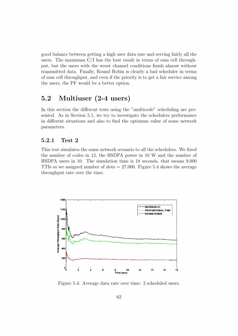
good balance between getting a high user data rate and serving fairly all theusers. The maximum C/I has the best result in terms of sum cell through-put, but the users with the worst channel conditions finish almost withouttransmitted data. Finally, Round Robin is clearly a bad scheduler in termsof sum cell throughput, and even if the priority is to get a fair service amongthe users, the PF would be a better option.

5.2 Multiuser (2-4 users)

In this section the different tests using the ”multicode” scheduling are pre-sented. As in Section 5.1, we try to investigate the schedulers performancein different situations and also to find the optimum value of some networkparameters.

5.2.1 Test 2

This test simulates the same network scenario to all the schedulers. We fixedthe number of codes in 12, the HSDPA power in 10 W and the number ofHSDPA users in 10. The simulation time is 18 seconds, that means 9.000TTIs so we assigned number of slots = 27.000. Figure 5.4 shows the averagethroughput rate over the time.


62

It shows the results of the three schedulers, and we can see that themaximum C/I is the algorithm which achieves the best throughput, but notso far away from the Proportional Fair. The RR has again the worst results.We can see that the average data rate is similar comparing it with the classicalway, because we increase the HSDPA power. If we would had simulated withthe same power, the average data rate would be lower.

5.2.2 Test 3

In this simulation we want to estimate the optimum value of the HSDPApower to maximize the total throughput rate. This test simulates only theMaximum C/I scheduling with 2 scheduled users. We fixed the number ofcodes in 12, the number of HSDPA users in 10 and the simulation time is6 seconds (that means 3.000 TTIs). The HSDPA power starts in 1 W andfinishes in 18 W. For this test the total power is 30 W. Figure 5.5 illustratesthe total data transmitted by each HSDPA power.

Figure 5.5: Total transmitted data over HSDPA power: 2 scheduled users.

Observing the Figure 5.5 we can determine that 12 W is the optimum HS-DPA power when 2 users are served. We could expect this result because

63

in the Figure 4.8 is shown that the optimum power in the HSDPA trafficwith only one served user is 6 W. Now in the multiuser scheduling, with 2served users, the result is logical. The test 8 shows the same simulation with4 served users.

5.2.3 Test 4

This test simulation is done under a manual user position assigment. Weonly simulate the maximum C/I scheduler because we try to demonstratethat very unfair scheduling mechanisms can lead to the starvation of theleast favourable users. We fixed the number of codes in 12, the HSDPApower in 14 W, the number of users is 10 and the simulation time is 10 sec-onds. The simulation is done with 3 scheduled users. Figure 5.6 illustratesthe users position, with 3 users in a good position and consequently withhigh probability of good channel conditions, and the rest of the users closeto the sector limit.

Figure 5.6: User position in test 4.

Figure 5.7 shows the individual data rate of the 10 users. We can see abig difference between the values obtained by the 3 users close to the base

64

station and the rest of the users.

Figure 5.7: Individual data rate: 3 scheduled users.

Thanks to this test we have checked that, using the maximum C/I scheduler,the users with the least favourable conditions can be highly ignored in thescheduling and the level of satisfaction among users could be poor.

5.2.4 Test 5

In this test the three schedulers are simulated with 3 scheduled users. Wefixed the HSDPA power in 14 W, the number of codes in 12, the number ofusers in 10 and the simulation time is 8 seconds. We simulate the HSDPAtraffic for 6 different Node-B distances, starting in 0.5 Km until 1.5 Km. Fig-ure 5.8 represents the average data rate as function of the Node-B distance.

The throughput rate decrease regularly when the Node-B distance is in-creased. As we can observe, the better results are obtained when the basestations are close, having not so good results when the distance is biggerthan 1 km. On the other hand, we can check again the schedulers perfor-mance: Round Robin has very bad results in terms of sum cell throughput,Maximum C/I and Proportional Fair have good results (MAX C/I slightly

65

Figure 5.8: Average data rate over distance: 3 scheduled users.

better), so considering the PF algorithm uses to be more fair, it should bethe selected option by the mobile operator.

5.2.5 Test 6

This test simulates the same network scenario to all the schedulers. We fixedthe number of codes in 12, the HSDPA power in 14 W and the number ofHSDPA users in 10. The simulation time is 18 seconds, that means 9.000TTIs so we assigned number of slots = 27.000. Figure 5.9 represents theaverage throughput rate over the time.

It shows the results of the three schedulers, and we can observe that, surpris-ingly, the highest average data rate occurs using PF algorithm. The possiblereason could be a higher BLER in the Maximum C/I, getting a worse rateeven thought the served users have the highest CQIs.

5.2.6 Test 7

In this simulation we want to estimate the optimum value of the HSDPApower to maximize the total throughput rate. This test simulates only theMaximum C/I scheduling with 4 scheduled users. We fixed the number of

66


codes in 12, the number of HSDPA users in 10 and the simulation time is6 seconds (that means 3.000 TTIs). The HSDPA power starts in 0 W andfinishes in 28 W. For this test the total power is 40 W (it is important tonote that most power amplifiers that are used today just support 20W, butwe change it in order to be able to find correctly the best HSDPA power).Figure 5.10 illustrates the total data transmitted by each HSDPA power.

Observing the Figure 5.10 we can see that 25 W is the optimum HSDPApower when 4 users are served. Again this result is logical compared withthe obtained values in the cases when 1 user (6 W) and 2 users (12 W) areserved. But we have to note that the total throughput in the interval [22-28W] is similar, so we cannot determine an absolute optimum value. In thiscase, it would be better to talk about an optimum HSDPA power interval.

67

Figure 5.10: Total transmitted data over HSDPA power: 4 scheduled users.

68

Chapter 6

Conclusions

This work has investigated the Packet Scheduling function in HSDPA, whichis a Third Generation (3G) mobile telephony communications protocol andthe evolution of UMTS/WCDMA. The goal of 3G systems is to provide usersnot only with the traditional circuit switched services, but also with newmultimedia services with high quality images and video for person-to-personcommunication, and with access to services and information in private andpublic networks.

The Packet Scheduling functionality plays a key role in HSDPA. The fea-tures included in HSDPA and the new location of the scheduler in the Node-B open new possibilities for the design of this functionality for the evolutionof WCDMA.

In this concluding chapter a summary of this bachelor thesis is given asfollows: Section 6.1 presents a short summary of the HSDPA simulator, try-ing to compile and clarify the exposed ideas about the simulator, especiallythe new functionality implemented to develop this bachelor thesis. In Sec-tion 6.2 a summary of the schedulers investigation and the simulator resultsis presented. Finally, Section 6.3 concludes this bachelor thesis describingsome possible uses of the simulator in future enhancements.

6.1 New Simulator Functionality

The MATLAB simulator developed by the Institute of Communications andRadio-Frequency of the Vienna University of Technology has been utilised to

69

develop this bachelor thesis. It consists in the simulation of a network withtwo mixed traffics: R’99 and HSDPA.

The initial purpose of this program was to evaluate the performance of thismixed network, testing the network with different combinations of the pa-rameters. Thus, this simulator could be also used to investigate the value ofthe parameters which maximize the overall throughput or the throughput ofone specific protocol (R’99 or HSDPA). As we have already explained, theinitial version utilizes a snapshot based simulation. The snapshot mode con-sists of (once the users and the network layout are created) realizing multiplesimulations of the network, changing the shadow and multipath fading as-signed to the users uncorrelated and randomly. So, after all the independentresults of each realisation are obtained, the mean over the realisations andthe users was calculated to finally obtain the global results.

Considering the static situation with the users in fixed positions and uncor-related fadings, it is not possible to simulate scheduling functions, based onserving at the users considering their radio conditions in previous moments,among other informations (i.e. in proportional fair, where it is necessary toknow the user average throughput).

As we have commented in Chapter 4, a new functionality was implementedin a existing HSDPA simulator to add the scheduling part in the simulations.We worked on the same basis, although some adjusts were done to achievethat besides snapshot based simulation also the enhanced time-based func-tionality could exist in the same program. The main modifications to get thenew functionality were done in the pathloss and shadow generation, in a waythat the simulation models utilised give back correlated in time values. Alsowe created new functions to simulate the users movement in the cell. Andthe most important part was the implementation of the schedulers whichwere investigated (Maximum C/I, Proportional Fair and Round Robin).

With the time-based functionality the simulator is more complete and give usa wide range of possible simulations. As we have seen in Chapter 5, we cansimulate more realistic situations besides the new possibility of investigatingthe schedulers.

70

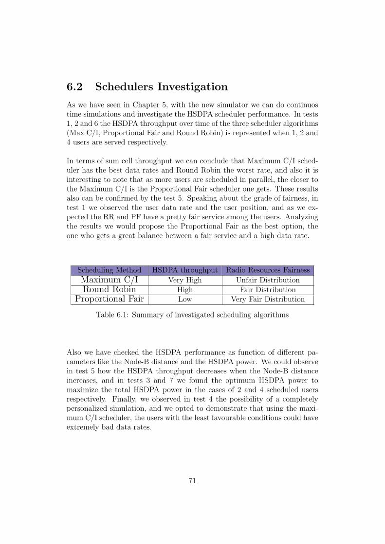
6.2 Schedulers Investigation

As we have seen in Chapter 5, with the new simulator we can do continuostime simulations and investigate the HSDPA scheduler performance. In tests1, 2 and 6 the HSDPA throughput over time of the three scheduler algorithms(Max C/I, Proportional Fair and Round Robin) is represented when 1, 2 and4 users are served respectively.

In terms of sum cell throughput we can conclude that Maximum C/I sched-uler has the best data rates and Round Robin the worst rate, and also it isinteresting to note that as more users are scheduled in parallel, the closer tothe Maximum C/I is the Proportional Fair scheduler one gets. These resultsalso can be confirmed by the test 5. Speaking about the grade of fairness, intest 1 we observed the user data rate and the user position, and as we ex-pected the RR and PF have a pretty fair service among the users. Analyzingthe results we would propose the Proportional Fair as the best option, theone who gets a great balance between a fair service and a high data rate.

Scheduling Method HSDPA throughput Radio Resources Fairness

Maximum C/I Very High Unfair DistributionRound Robin High Fair Distribution

Proportional Fair Low Very Fair Distribution

Table 6.1: Summary of investigated scheduling algorithms

Also we have checked the HSDPA performance as function of different pa-rameters like the Node-B distance and the HSDPA power. We could observein test 5 how the HSDPA throughput decreases when the Node-B distanceincreases, and in tests 3 and 7 we found the optimum HSDPA power tomaximize the total HSDPA power in the cases of 2 and 4 scheduled usersrespectively. Finally, we observed in test 4 the possibility of a completelypersonalized simulation, and we opted to demonstrate that using the maxi-mum C/I scheduler, the users with the least favourable conditions could haveextremely bad data rates.

71

6.3 Future Enhancements

In this bachelor thesis only some possibilities of the new simulator have beenexplored. During the development of this work was conducted to introducereal data network in the simulation. Accordingly, combining both parts thesimulator will be even more realistic. On the other hand, it would be inter-esting to add to the simulator some HSDPA technologies that still are notincorporated like the H-ARQ.

In addition, I would like to present a short introduction to HSPA Evolved,also known as HSPA+. I would propose that a possible enhancement of thesimulator could be to adapt it to evaluate the performance of the new tech-nologies introduced by HSPA+.

HSPA+ is the next step and is more focused on delivering data servicesenabling speeds of up to 25 Mbps in the downlink and 11 Mbps in the up-link, [6]. It uses MIMO technologies and higher order modulation. It alsointroduces an optional all-IP architecture for the network where base stationsare directly connected to the internet. Several trials are underway and thefirst commercial launches have been announced for late 2008. On 10 June,2008 Australia’s Next G was the first network to enable some features ofHSPA+, [48].

System level investigations on this topic have already started, [49], [50], [51],[52] and [53], but for sure many more interesting results will follow.

72

Bibliography

[1] Yahong Rosa Zheng and Chengshan Xiao. ”Simulation models with cor-rect statistical properties for Rayleigh fading channels”. IEEE Transac-tions on Communications, Vol. 51, No. 6, June 2003.

[2] C.Fragouli, V. Sivaraman, and M. Srivastava. ”Controlled multimediawireless link sharing via enhanced class-based queueing with channel-state dependent packet”. IN-FOCOM98, vol. 2. March 1998.

[3] Li Wang, Yu-Kwong Kwok, Wing-Cheong Lau, and Vincent K. N. Lau.”Channel Capacity Fair Queueing in Wireless Networks: Issues and aNew Algorithm”. ICC 2002. April 2002.

[4] M. Andrews, K. Kumaran, K. Ramanan, A. Stolyar, P. Whiting, and R.Vijayakumar. ”Providing quality of service over a shared wireless link”.IEEE Communications Magazine. Feb. 2001.

[5] S. Lu and V. Bharghavan. ”Fair scheduling in wireless packet networks”.IEEE Trans. Networking. 1999.

[6] HSPA Mobile Broadband Today (http://www.gsmworld.com)

[7] Harri Holma and Antti Toskala. HSDPA/HSUPA for UMTS: High SpeedRadio Access for Mobile Communications. John Wiley & Sons. June2006.

[8] Walsh Code from Wikipedia (http://en.wikipedia.org/wiki/Walshcode)

[9] 3GPP. Technical Specification Group Radio Access Network. MAC Pro-tocol Specification. (3GPP TS 25.321 version 5.1.0).

[10] 3GPP. Technical Specification Group Radio Access Network. High-Speed Downlink Packet Access (HSDPA); Overall Description. (3GPPTS 25.308 version 5.4.0).

73

[11] Pablo Amiegeiras Gutierrez. ”Packet Scheduling And Quality of Servicein HSDPA”. Ph. D. Thesis. October 2003.

[12] Chase D. ”Code Combining: A Maximum Likelihood Decoding Ap-proach for Combining an Arbitrary Number of Noise Packets”. Commu-nications, IEEE Trans. Vol. 33. May 1985.

[13] Stevens R. ”TCP/IP Illustrated”. Volume 1. The Protocols. AddisonWesley, 1994.

[14] 3GPP. Technical Specification Group Radio Access Network. UTRANIub Interface NBAP signalling. (3GPP TR 25.433 version 5.5.0).

[15] 3GPP. Technical Specification Group Radio Access Network. UTRANIub Interface User Plane Protocols for Common Transport Channel DataStreams. (3GPP TS 25.435 version 5.4.0).

[16] Elliott R.C. et al. ”Scheduling Algorithms for the CDMA2000 PacketData Evolution”. Vehicular Technology Conference. 2002.

[17] D. Bertsekas, Gallager R. Data Networks. Second Edition. Prentice Hall.1992.

[18] Kolding T. et al. ”Performance Aspects of WCDMA Systems with HighSpeed Downlink Packet Access (HSDPA)”. Vehicular Technology Con-ference, 2002. VTC 2002 Fall. Volume 1. pp. 477-481.

[19] Martin Wrulich, Werner Weiler and Markus Rupp. ”HSDPA Perfor-mance in a Mixed Traffic Network”. Proc. 2008 IEEE 67th VehicularTechnology Conference. Singapore. May 2008.

[20] 3GPP. Technical Specification Group Radio Access Network. Multiple-Input Multiple Output Antenna Processing for HSDPA. (3GPP TR25.876 version ).

[21] Recommendation ITU-R P.1407. ”Multipath propagation and parame-terization of its characteristics”. 1999.

[22] Members of COST 231. ”Digital mobile radio towards future generationsystems - COST 231 final report”. COST, Tech. Reo., 1999.

[23] A.Seeger, M.Sikora, and A.Klein. ”Variable Orthogonality factor: a sim-ple interface between link and system level simulation for high speeddownlink packet access”. Proc. of the IEEE Vehicular Technology Con-ference 2003. Oct. 2003.

74

[24] F.Brouwer, I. de Bruin, J.Silva, N.Souto, F.Cercas, and A.Correia. ”Us-age of link-level performance indicators for HSDPA network-level sim-ulations in E-UMTS”. Proc. of the Eight Internationsl Symposium onSpread Spectrum Techniques and Applications. Sept. 2004.

[25] 3GPP. Technical Specification Group Radio Access Network. Physicallayer procedures (FDD)(Release 7). (3GPP TS 25.214 version 7.6.0).

[26] R.Litjens. ”HSDPA flow level performance and the impact of terminalmobility”. Proc. of the Wireless Communications and Networking Con-ference. Mar.2005.

[27] K.Sipila, K.-C. Honkasalo, J. Laiho-Steffens, ad A.Wacker. ”Estimationof capacity and required transmission power of WCDMA downlink basedon a downlink pole equation”. Proc. of the IEEE Vehicular TechnologyConference 2000. May 2000.

[28] John G. Proakis. Digital Communications, 3rd edition, Singapore:McGraw-Hill Book Co. 1995.

[29] R. H. Clarke. ”A Statistical Theory of Mobile-Radio Reception”. Bellsyst. Tech. J. Jul-Aug 1968.

[30] William C. Jakes. Microwave Mobile Communications. New York: JohnWiley & Sons Inc. Feb.1975.

[31] P.Dent, G. E. Bottomley, and T.Croft. ”Jakes fading model revisited”.Electron. Lett. June 1993.

[32] M.Patzold, U. Killat, F. Laue, and Y. Li. ”On the Statistical Proportiesof Deterministic Simulation Models for Mobile Fading Channels”. IEEETrans. Veh. Technol. Feb.1998.

[33] Y. X. Li and X. Hunag. ”The Simulation of Independent RayleighFaders”. IEEE Trans. Commun. Sept. 2002.

[34] Thomas Zemen and Christopher Mecklenbrauker. ”Time-variant chan-nel estimation using discrete prolate spheroidal sequences”. IEEE Trans-actions on signal processing, Vol. 53, No.9, September 2005.

[35] M. F. Pop and N. C. Beaulieu. ”Limitations of sum-of-simusoids fadingchannel simulators”. IEEE Trans. Commun. April 2001.

75

[36] C. Xiao, Y. R. Zheng, and N. C. Beaulie. ”Second-order statistical pro-porties of the WSS Jakes’ fading channel simulator”. IEEE Trans. Com-mun. June 2002.

[37] Thomas Zemen and Christopher Mecklenbrauker. ”Doppler diversity inMC-CDMA using the Slepian basis expansion model”. Proc. 12th EUR.Signal Process. Conf,. Vienna, Austria, Sep. 2004.

[38] Gudmundson, M. ”Correlation Model for Shadow Fading in Mobile Ra-dio Systems”. Electronics Letters, Vol. 27, No.23, November 1991.

[39] Aun Haider and Richard Harris. ”A Novel Proportional Fair SchedulingAlgorithm for HSDPA in UMTS Networks”. The 2nd International Con-ference on Wireless Broadband and Ultra Wideband Communications(AusWireless 2007).

[40] F.Kelly. ”Charging and Rate Control of Elastic Traffic”. Eu-ropean Transactions on Telecommunications. 8:33-37, 1997.http://www.statslab.cam.ac.uk/ frank/elastic.html.

[41] M.Assaad and D.Zeghlache. ”Scheduling Study in HSDPA System”.IEEE 16th International Sysmposium on Personal, Indoor and MobileRadio Communications. 2005.

[42] Lin Yang, Ming Kang, and Mohamed-Slim Alouini. ”On the Capacity-Fairness Tradeoff in Multiuser Diversity Systems”. IEEE Transactionson Vehicular Technology. Vol.56. Nr. 4. July 2007.

[43] Kinda Khawam. ”The Modified Proportional Fair Scheduler”. 17th An-nual IEEE International Sysmposium on Personal, Indoor and MobileRadio Communications. 2006.

[44] Hua Fu and Dong In Kim. ”Analysis of Throughput and Fairness withDownlink Scheduling in WCDMA Networks”. IEEE Transactions onWireless Communications. Vol.5. Nr. 8. August 2006.

[45] Soo-Yong Jeon. ”An Enhanced Channel-Quality Indication (CQI) Re-porting Scheme for HSDPA Systems”. IEEE Communications Letters.Vol. 9. No. 5. May 2005.

[46] A.Jalali, R.Padovani, and R.Pankaj. ”Data throughput of CDMA-HDRa High Efficiency-High Data Rate Personal Communication WirelessSystem”. Proc. of IEEE VTC 2000, 3:1854-1858, 2000.

76

[47] D.Yang, D.Shen, W.Shao, and V.Li. ”Towards Opportunistic FairScheduling in Wireless Networks”. Proc. of IEEE ICC, 5217-5221. June2006.

[48] Ericsson world-first in delivering innovative 3G technology to Tel-stra (http://www.ericsson.com/ericsson/press/releases/20080610-1226569.shtml)

[49] M. Wrulich, C. Mehlfuhrer and M. Rupp. ”Interference Aware MMSEEqualization for MIMO TxAA”. Proc. of IEEE 3rd International Sym-posium on Communications, Control and Signal Processing (ISCCSP).1585-1589. 2008.

[50] C. Mehlfuhrer, M. Wrulich and M. Rupp. ”Intra-cell Interference AwareEqualization for TxAA HSDPA”. Proc. of IEEE 3rd International Sym-posium on Wireless Pervasive Computing. 406-409. 2008

[51] C. Mehlfuhrer, S. Caban, M. Wrulich and M. Rupp. ”Joint ThroughputOptimized CQI and Precoding Weight Calculation for MIMO HSDPA”.Conference Record of the Fourtysecond Asilomar on Signals, Systemsand Computers. Oct. 2008.

[52] M. Wrulich and M. Rupp. ”Efficient Link Measurement Model for Sys-tem Level Simulations of Alamouti Encoded MIMO HSDPA Transmis-sions”. International (ITG) Workshop on Smart Antennas (WSA). Feb.2008.

[53] M. Wrulich, S. Eder, I. Viering and M. Rupp. ”Efficient Link-to-SystemLevel Model for MIMO HSDPA”. Proc. of the 4th IEEE BroadbandWireless Access Workshop. 2008.

77

Bachelor Thesis INVESTIGATION OF HSDPA SCHEDULERS

Documents

Transcript of Bachelor Thesis INVESTIGATION OF HSDPA SCHEDULERS