Bachelor thesis - cyber.felk.cvut.cz
47
CZECH TECHNICAL UNIVERSITY IN PRAGUE Faculty of Electrical Engineering Bachelor thesis Jan Langr Odor source localization using swarm of unmanned helicopters Department of Cybernetics Thesis supervisor: Ing. Martin Saska, Dr. rer. nat.
Transcript of Bachelor thesis - cyber.felk.cvut.cz

CZECH TECHNICAL UNIVERSITY IN PRAGUE
Faculty of Electrical Engineering
Bachelor thesis
Jan Langr
Odor source localization using swarm of unmannedhelicopters
Department of Cybernetics
Thesis supervisor: Ing. Martin Saska, Dr. rer. nat.


Acknowledgement
I would like to thank Dr. Martin Saska for his help and useful tips throughout this work.

Abstrakt
Cılem teto prace je modifikovat zakladnı PSO algoritmus pro ucel nale-zenı zdroje koure pomocı roje bezpilotnıch helikopter. Jelikoz PSO al-goritmus vyzaduje, aby clenove roje znali svou pozici v prostoru, musıbyt vybrano a vyuzito nekolik moznostı absolutnı lokalizace. V zajmuzabranenı kolizım clenu roje musı take byt pouzit prostredek relativnılokalizace robotu. Nejprve bude implementovana zakladnı verze PSO al-goritmu s jednoduchou hodnoticı funkcı bez uvazenı jakychkoliv ome-zenı. Po naladenı parametru algoritmu bude aplikovan na nalezenı zdrojekoure a dale testovan. Pote budou implementovany modifikace algoritmuzohlednujıcı omezenı realnych robotu (kvadrukopter) a algoritmus budeopet testovan s jednoduchou hodnoticı funkcı. Ve vysledku budou veskeremodifikace spojene do jednoho algoritmu, ktery bude zamereny na loka-lizaci zdroje koure a zaroven bude zohlednovat omezenı dana realnymiroboty.

Abstract
The goal of this thesis is to modify the Particle Swarm Optimizationalgorithm to allow its use with small UAVs and utilize it for the taskof locating the source of a smoke. Since the PSO algorithm requires theswarm individuals to know their immediate position, several means ofabsolute localization of the robots have to be devised and used. In orderto avoid collisions, a means of relative robot localization must be used.First, a simple version of the PSO algorithm using particles with noconstraints will be used in combination with a simple fitness function.After tuning the algorithm’s parameters, it will be used to find a sourceof a smoke and further tested. Then, the PSO algorithm modified usingthe real quadrotor constraints will be tested with the same basic fitnessfunction. Eventually, the combination of these two apporaches will yieldan algorithm applicable on real quadrotors and the task of locating asmoke source.

CONTENTS
Contents
1 Introduction 1
2 Related work 2
3 Simulation environment 3
3.1 Fitness function . . . . . . . . . . . . . . . . . . . . . . . . . . . . . . . . . 3
3.2 Used symbols . . . . . . . . . . . . . . . . . . . . . . . . . . . . . . . . . . 4
4 Quadrotor helicopter model and regulator 5
4.1 Dynamic model . . . . . . . . . . . . . . . . . . . . . . . . . . . . . . . . . 6
4.2 Regulator . . . . . . . . . . . . . . . . . . . . . . . . . . . . . . . . . . . . 7
5 Means of localization 10
5.1 Absolute localization . . . . . . . . . . . . . . . . . . . . . . . . . . . . . . 10
5.2 Relative localization . . . . . . . . . . . . . . . . . . . . . . . . . . . . . . 11
6 Odor model 13
6.1 Smoke particle . . . . . . . . . . . . . . . . . . . . . . . . . . . . . . . . . . 13
6.2 Smoke density grid . . . . . . . . . . . . . . . . . . . . . . . . . . . . . . . 13
6.3 Smoke particle dynamics . . . . . . . . . . . . . . . . . . . . . . . . . . . . 14
7 PSO algorithm implementations 17
7.1 Basic PSO algorithm . . . . . . . . . . . . . . . . . . . . . . . . . . . . . . 18
7.1.1 Simulation setup . . . . . . . . . . . . . . . . . . . . . . . . . . . . 18
7.1.2 Fitness function . . . . . . . . . . . . . . . . . . . . . . . . . . . . . 18
7.1.3 Simulation results . . . . . . . . . . . . . . . . . . . . . . . . . . . . 19
7.2 Basic PSO algorithm for smoke source localization . . . . . . . . . . . . . . 21
7.2.1 Simulation setup . . . . . . . . . . . . . . . . . . . . . . . . . . . . 21
7.2.2 Fitness function . . . . . . . . . . . . . . . . . . . . . . . . . . . . . 21
7.2.3 PSO algorithm modifications . . . . . . . . . . . . . . . . . . . . . 21
7.2.4 Smoke source location prediction . . . . . . . . . . . . . . . . . . . 22
7.2.5 Simulation results . . . . . . . . . . . . . . . . . . . . . . . . . . . . 23
7.3 PSO algorithm with collision avoidance . . . . . . . . . . . . . . . . . . . . 25
i

CONTENTS
7.3.1 Simulation setup . . . . . . . . . . . . . . . . . . . . . . . . . . . . 25
7.3.2 Fitness function . . . . . . . . . . . . . . . . . . . . . . . . . . . . . 25
7.3.3 PSO algorithm modifications . . . . . . . . . . . . . . . . . . . . . 25
7.3.4 Simulation results . . . . . . . . . . . . . . . . . . . . . . . . . . . . 28
7.4 Final PSO algorithm for smoke source localization . . . . . . . . . . . . . . 30
7.4.1 Simulation setup . . . . . . . . . . . . . . . . . . . . . . . . . . . . 30
7.4.2 Simulation results . . . . . . . . . . . . . . . . . . . . . . . . . . . . 30
8 Conclusion 32
9 Appendix 34
9.1 CD Contents . . . . . . . . . . . . . . . . . . . . . . . . . . . . . . . . . . 34
ii

LIST OF FIGURES
List of figures
1 View of the simulation environment with 2 quadrotors . . . . . . . . . . . 3
2 Used simulation symbols . . . . . . . . . . . . . . . . . . . . . . . . . . . . 4
3 Quadrotor with a foam protection frame [1] . . . . . . . . . . . . . . . . . 5
4 Quadrotor model with used reference frames [2] . . . . . . . . . . . . . . . 6
5 The camera setup with its field of view and a pattern [3] . . . . . . . . . . 11
6 The camera and blob properties used to determine the blob’s visibility . . 12
7 2D analogy of the implemented smoke concentration mechanism . . . . . . 14
8 Simulation environment with one smoke source . . . . . . . . . . . . . . . . 16
9 Basic PSO algorithm with a simple fitness function . . . . . . . . . . . . . 20
10 PSO algorithm modified for locating a smoke source . . . . . . . . . . . . . 24
11 PSO algorithm with a simple fitness function using robot relative localization 29
12 Final PSO algorithm for smoke source localization with collision avoidance 31
iii

LIST OF TABLES
List of tables
1 Parameter values of the basic PSO algorithm . . . . . . . . . . . . . . . . . 18
2 Parameter values of the basic smoke source searching PSO algorithm . . . 23
3 Parameter values of the PSO algorithm with collision avoidance . . . . . . 28
4 Parameter values of the final PSO implementation . . . . . . . . . . . . . . 30
5 CD contents . . . . . . . . . . . . . . . . . . . . . . . . . . . . . . . . . . . 34
iv

LIST OF ALGORITHMS
List of algorithms
1 Algorithm of a single smoke step . . . . . . . . . . . . . . . . . . . . . . . . 15
2 Algorithm for calculating non-colliding new positions of robots . . . . . . . 27
v

1 Introduction
One of the aims of mobile robotics and artificial intelligence is to substitute a humanbeing in performing certain tasks. This may be especially useful if the performed taskpresents a health risk. For instance, locating and neutralizing a gas leakage that could atany moment cause an explosion or lead to suffocation or intoxication of people. The aimof this work is to study whether the use of flying automated robots behaving according tothe rules of a modified PSO algorithm can be used to perform this precise task.
In this work, several separate steps will be followed in order to achieve the given goal. Atfirst, a simple version of the PSO algorithm with an easy-to-visualize fitness function willbe implemented. This will help in fine-tuning the algorithm’s parameters. After assuringthe algorithm’s convergence, a dynamic model of smoke will be implemented along witha fitness function that will allow a successful location of the source of the smoke. Thebasic PSO algorithm will then be applied in a confined space containing the smoke andits source. At this point, the algorithm may already need some modifications due to thespecific nature of the measured fitness function.
Next, all constraints and limitations of a quadrotor UAV will be considered. This inclu-des its non-zero dimensions, wind funnels created by rotors, and, mainly, the implicitinability to know its immediate position. For position tracking, several types of sensorswill be implemented into the simulation. For relative localization of swarm members, acamera system that is currently being developed by the Department of Cybernetics will beused. For absolute vertical localization of the robots, barometric, ultrasonic or laser (or acombination of these) altimeters could prove effective, and for localization in the horizon-tal plane, a camera together with an algorithm computing the optical flow of the camera’spicture will be used.
Eventually, the basic PSO algorithm will be modified to take into account the mentionedlimitations. After functionality of this version of the algorithm reaches a sufficient level,it will be used to successfully locate the source of a smoke. The performance of the finalalgorithm will then be evaluated based on observation and compared to the performanceof the basic version of the algorithm.
1/34

2 Related work
Paper [4] deals with the task of locating a plume source under water with an AUV(autonomous underwater vehicle). Two approaches at locating the source of a plume arepresented. The first approach causes the vehicle to trace the plume to its source. The secondapproach uses an algorithm to estimate the location of the source based on measured con-centration of the plume and water flow at different spots. It is stated that for environmentswith a low Reynolds number (ratio of inertial forces to viscous forces in a fluid) wherelaminar flow is prevalent, a gradient-type searching algorithm can be employed. However,for environments with a large amount of turbulences where the direction of fluid flow doesnot give correct information about the source of the plume, a gradient following approachis not suited. Since a plume with prevalent laminar flow will be considered in this work, thePSO algorithm seems to be a reasonable choice, because it is a type of gradient-followingalgorithm.
2/34

3 Simulation environment
Throughout this entire work, the operation area for the robot swarm will stay the same.It is a cuboid 16 meters wide, 16 meters deep and 9 meters high. The area contains noobstacles. In each plot showing the progress of an algorithm, one view from the top andtwo views from the side of the operation area are be shown. The robots’ movement is notlimited to this area, but the new positions calculated in each iteration of the PSO algorithmare be located within the boundaries of this cuboid. This is to assure all-time visibility ofthe swarm members in the plot, but allow occasional crossing of the boundaries due to therobots’ inertia. An example of a plot of the operation area is in figure 1.
Figure 1: View of the simulation environment with 2 quadrotors
3.1 Fitness function
One of the main parts of the PSO algorithm is a fitness function, whose values serveas the input of the algorithm. Its value is a function of spatial coordinates (mainly) andtime. The operation area is divided into a grid of cubical cells of small size. Each of thesecells can contain a value calculated from the cell’s x, y and z coordinates (and optionallytime) using the fitness function’s formula. The reason why a discrete cell grid instead of acontinuous space is chosen to store the values is explained in chapter 6.2.
3/34

3.2 Used symbols
3.2 Used symbols
The following symbols are used in the visual representation of the simulation progress:
Figure 2: Used simulation symbols
4/34

4 Quadrotor helicopter model and regulator
Since smoke generally spreads both horizontally and vertically, the use of ground robotsis not possible. A possible exception would be smoke released in an operation area of verylow height, where the wind velocity and concentration of the gas at position [x, y, 0] wouldbe roughly equal to the values measured at position [x, y, zmax]. The robot type used toachieve the goal of this work has to be able to travel not only on the ground surface of theoperation area, but also in the vertical direction.
The quadrotor helicopter is a type of aerial vehicle frequently used for robotic purposes.An example of a quadrotor can be seen in figure 3. The presence of four rotors, instead of alarge one used in standard helicopters, allows the use of much smaller and cheaper propellersless prone to being damaged. In combination with a foam guarding frame surrounding therotors, the quadrotor is a durable aerial vehicle well suited for robotic experiments whereaccidents are expected. Also, its symmetry allows for equipment installation on all four sidesequally (for example cameras, special markers for recognition by other cameras, sensorsetc.).
Figure 3: Quadrotor with a foam protection frame [1]
5/34

4.1 Dynamic model
4.1 Dynamic model
To simulate realistic movement of the quadrotor, the dynamic model and regulatorpresented in [2] will be used. First, two reference frames are introduced to describe the state
of the quadrotor, as seen in figure 4. The coordinate system ~i1,~i2,~i3 is an inertial reference
frame connected to the operation area of the robot. The coordinate system ~b1, ~b2, ~b3is connected to the body of the quadrotor with its origin in the center of mass of thequadrotor. The vectors ~b1 and ~b2 lie in the plane defined by the four centers of propellers,the ~b3 vector is perpendicular to this plane. In later chapters, the ~b1 vector is used toindicate the ’front’ of the robot.
Figure 4: Quadrotor model with used reference frames [2]
Let us define the following variables [2]:
m ∈ R the total mass of the quadrotorJ ∈ R3×3 the inertia matrix with respect to the body-fixed frameR ∈ SO(3) the rotation matrix from the body-fixed frame to the inertial frame~Ω ∈ R3 the angular velocity in the body-fixed frame~x ∈ R3 the location of the quadrotor’s center of mass in the inertial frame~v ∈ R3 the velocity of the quadrotor’s center of mass in the inertial framed ∈ R the distance from the center of mass to the center of each rotor
fi ∈ R the thrust generated by the i-th propeller along the −~b3 axis
τi ∈ R the torque generated by the i-th propeller about the −~b3 axisf ∈ R the total thrust (Σ4
i=1fi)M ∈ R the total moment in the body-fixed frame
6/34

4.2 Regulator
4.2 Regulator
The following equations describe the quadrotor’s motion:
~x = ~v (1)
m~v = mg~e3 − fR~e3 (2)
R = RΩ (3)
JΩ + Ω× JΩ = M (4)
First, the position and velocity tracking errors are calculated:
~ex = ~x− ~xd (5)
~ev = ~v− ~vd (6)
(7)
where the subscript d denotes the desired value of a variable. The desired direction ofthe ~b3 vector is calculated:
~b3d = − −kx~ex − kv~ev −mg~e3
|−kx~ex − kv~ev −mg~e3|(8)
Using the ~b1d vector, which is also the regulator’s input, ~b2d and Rd are calculated:
~b2d =(~b3d × ~b1d)∣∣∣~b3d × ~b1d
∣∣∣ (9)
Rd =[~b2d × ~b3d, ~b2d, ~b3d
](10)
Then, the rotation matrix and angular velocity matrix errors are calculated:
~eR =1
2(RT
dR−RTRd)∨ (11)
~eΩ = ~Ω−RTRd~Ωd (12)
7/34

4.2 Regulator
Finally, the total force and moments are calculated:
f = −(−kx~ex − kv~ev −mg~e3)R~e3 (13)
M = −kR~eR − kΩ~eΩ + ~Ω× J~Ω− J(~ΩRTRd~Ωd −RTRd
~Ωd) (14)
To limit the maximum thrust of the propellers, the following equation is used:fM1
M2
M3
=
1 1 1 10 −d 0 dd 0 −d 0−cτf cτf −cτf cτf
·
f1
f2
f3
f4
(15)
Values f1 through f4 are expressed from the equation, attenuated according to themaximum thrust of each propeller, and plugged back into the equation to obtain the finalforce and moments. The new velocity, position and rotation of the quadrotor are thencalculated. Since the regulator calculates the trajectory’s discrete steps, step time ∆t isdefined:
~vnew =∆t
m(mg~e3 − fR~e3) + ~v (16)
~xnew = ~vnew + ~x (17)
~Ωnew = J−1(M − ~Ω× J~Ω) (18)
Rnew = RRω (19)
where
Rω = 1 + (1− cos(a))(ω2x − 1) ωz sin(a) + (1− cos(a))ωxωy ωy sin(a) + (1− cos(a))ωxωz
−ωz sin(a) + (1− cos(a))ωxωy 1 + (1− cos(a))(ω2y − 1) −ωx sin(a) + (1− cos(a))ωyωz
−ωy sin(a) + (1− cos(a))ωxωz ωx sin(a) + (1− cos(a))ωyωz 1 + (1− cos(a))(ω2z − 1)
ωx = Ω(1)
ωy = Ω(2)
ωz = Ω(3)
a = ∆t · |Ω|
8/34

4.2 Regulator
The used constants have the following values:
parameter value unitsm 4.34 kgkx 6.32 –kv 7.6 –kR 19.81 –kΩ 2.54 –g -9.81 m · s−2
∆t 0.005 s
J =
0.082 0 00 0.0845 00 0 0.1377
9/34

5 Means of localization
In order for the swarm to navigate correctly through the operation environment, a meansof absolute and relative localization of the swarm members must be present. This is forthree reasons:
• In order to calculate the trajectories of the swarm members, the PSO algorithm needsto know their absolute position (position in the operation environment’s referenceframe) and the position of their measured personal best value of the fitness function.
• The members need to be able to tell the location of the located target in the operationarea’s reference frame.
• The robots must have the ability to detect imminent collisions with the environmentand themselves, and avoid such collisions.
5.1 Absolute localization
Not only need the robots know their position in the environment, they also need tohave information about their complete state. That includes the rotation of the body-fixedreference frame in the inertial reference frame. Several types of sensors may serve as sourcesof information about the state of the quadrotor:
• An optical flow sensor pointed towards the ground could serve as a sensor ofdisplacement in the horizontal plane of the inertial reference frame. To compensatefor the quadrotor’s pitch and roll, the sensor could be mounted on a (motorized) ballpivot.
• In addition to the optical flow sensor, accelerometers could be mounted to measurethe robot’s movement.
• To calculate the direction of the ~b1 vector, a gyroscope (or multiple gyroscopes)could be mounted on the quadrotor. An alternative to this would be an accelerometerattached in a place far from the robot’s center of mass. That way, the accelerationof a point on the circumference of the robot would be measured, which would, afterdouble integration, yield the robot’s rotation about the axis given by ~b3.
• To measure the altitude of the robot, a barometric altimeter (inaccurate) in com-bination with an ultrasonic or laser altimeter could be used.
The task of acquiring reliable means of the quadrotor’s absolute localization is a complexone. The sensors mentioned earlier for horizontal position measuring produce additiveerrors, which would after a period of time lead to a difference between the actual robot’s
10/34
5.2 Relative localization
position and the position calculated by the robot itself. The measured altitude of the robotwould be altered by any object on the ground of the operation area, which would leadto rapid altitude changes of the robot (in effort to maintain a desired altitude above ameasured point). All the errors above mentioned could be reduced using relative cameralocalization of the robots and fusion of data from multiple cameras.
For the sake of the goal this work aims to achieve, let us assume that the robots knowtheir absolute position and rotation with precision. Also, the operation area will not containany obstacles or walls, and the ground will be flat.
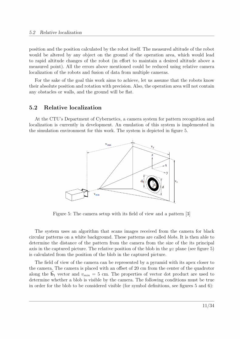
5.2 Relative localization
At the CTU’s Department of Cybernetics, a camera system for pattern recognition andlocalization is currently in development. An emulation of this system is implemented inthe simulation environment for this work. The system is depicted in figure 5.
Figure 5: The camera setup with its field of view and a pattern [3]
The system uses an algorithm that scans images received from the camera for blackcircular patterns on a white background. These patterns are called blobs. It is then able todetermine the distance of the pattern from the camera from the size of the its principalaxis in the captured picture. The relative position of the blob in the yz plane (see figure 5)is calculated from the position of the blob in the captured picture.
The field of view of the camera can be represented by a pyramid with its apex closer tothe camera. The camera is placed with an offset of 20 cm from the center of the quadrotoralong the ~b1 vector and vmin = 5 cm. The properties of vector dot product are used todetermine whether a blob is visible by the camera. The following conditions must be truein order for the blob to be considered visible (for symbol definitions, see figures 5 and 6):
11/34

5.2 Relative localization
~d · ~b1
|~d||~b1|> 0 (20)∣∣∣|~d| cos(α)
∣∣∣ <= vmax − vmin (21)∣∣∣|~d| cos(β)∣∣∣ <=
∣∣∣|~d| cos(α)∣∣∣ wmaxvmax − vmin
(22)∣∣∣|~d| cos(γ)∣∣∣ <=
∣∣∣|~d| cos(α)∣∣∣ hmaxvmax − vmin
(23)
~nblob · ~b1
|~nblob||~b1|< cos(π − blobAnglemax) (24)
where blobAnglemax is the maximum angle in degrees allowed betwen the ~nblob vectorand the yz plane’s normal vector (pointing towards the camera).
Equation 20 guarantees that the blob is in front of the camera and ’below’ the pyramid’sapex. Equation 21 limits the blob’s distance from the camera. Equations 22 and 23 gua-rantee the blob is within the pyramid’s boundaries in the yz plane. And finally, equation24 only makes the blob visible if the angle between its normal vector and the yz plane’snormal vector is less than blobAnglemax.
Figure 6: The camera and blob properties used to determine the blob’s visibility
If all the above conditions are satisfied, the blob is considered visible for the quadrotorowning the camera, and its exact position is know by this quadrotor. The system allowsfor either the detection of a single blob or multiple blobs. Also, if the blobs are equippedwith an additional unique marking symbol, the camera system is able to distinguish them.Some of these possibilities are exploited in chapter 7.
12/34

6 Odor model
For the specific application of the PSO algorithm this work deals with, the localization ofan odor source, a sufficiently accurate dynamic model of smoke has to be implemented. Thatincludes the movement of emitted particles, the effect of wind acting upon the particlesand possibly changes from laminar to turbulent air flow. Since the algorithm aims to locatea point or a small area in the operation space where the value of the cost function has itsmaximum (or minimum), a smoke source of small dimensions has to be used. Therefore,after the algorithm is finished, it will not be applicable on large scale smoke sources suchas wildfires, but on locating smaller smoke sources (gas leakage through a hole in a pipe).In this version of the simulation, the smoke source has zero dimensions, which means theparticles are all emitted from the same point in the operation space.
6.1 Smoke particle
An individual smoke particle has the following parameters:
• [x, y, z] - position coordinates in the operation space
• [vx, vy, vz] - velocities along the respective axes of the operation space coordinatesystem
• [vxinit, vyinit
, vzinit] - initial velocities at the moment of emission
• lifetime - the time passed since the particle’s emission (more precisely the number ofposition changes the particle has undergone)
All the particles share the same value of a parameter called maximum lifetime, whichsays how many position changes each particle can go through before it is recycled. This isexplained in chapter 6.3.
6.2 Smoke density grid
Since gas concentration sensors are used by the robots to ’measure’ the smoke in differentparts of the area, a means of determining the smoke density at a given point in space hasto be devised. Because the smoke consists of a massive amount of particles (thousands totens of thousands), the method must not be computationally complex. One way would beto calculate the distance of each particle from the sensor and compare it to a thresholdvalue. The number of particles with distance smaller than this threshold value would thenbe considered as the smoke density at that point. This would, however, cause a significantload to the computer and decrease the framerate of the simulation.
13/34

6.3 Smoke particle dynamics
As mentioned in chapter 3.1, a grid of discrete cubical cells filling the operation area isused to store the values of the cost function. The density at the location of the smoke sensorwill simply be represented by the number of particles enclosed in the same cell where thesensor is located. As each particle leaves a cell, the cell’s value will decrease by one. As itenters a new cell, the new cell’s value will increase by one. A visual example is in figure 7.
Figure 7: 2D analogy of the implemented smoke concentration mechanism
6.3 Smoke particle dynamics
The last step is to create a set of rules for the particles to obey in order to sufficientlyresemble real smoke. Smoke in an air-filled area consists of small solid particles beingcarried away by molecules of air, or simply by molecules of a gas other than air.
Once emitted, these molecules are accelerated by moving molecules of air around them(wind). If a wind of constant velocity is considered, the smoke particles are acted upon bya constant force, which causes constant velocity increments in each discrete time step. Ineach time step, the particle is accelerated until it matches the velocity of the wind at itslocation. Additionally, a small random vector is added to the particle’s calculated velocityvector to break the smoke’s uniformity.
The simulation can only deal with a limited number of particles. To avoid the need ofconstantly creating new particles and dismissing old ones, particles are recycled. In theinitial stage, new particles are emitted into the area. Once the maximum allowed numberof particles is reached, no new particles are released, and the oldest ones are relocatedback at the location of the smoke source with their initial velocity. If particles are releasedfrom the source in waves, the maximum number of steps a particle can undergo is given bymaxParticles/particleWave, where particleWave is the number of particles emitted ineach time step. This effectively yields a continuous smoke. Algorithm 1 shows the policy of
14/34

6.3 Smoke particle dynamics
smoke particle movement. A visualisation of the smoke in the operation area can be seenin figure 8.
For a smoke source located at [sx, sy, sz] :if existingParticles < maxParticles then
for i = 0; i ≤ particleWave docreate new particle;densityGrid [xs, ys, zs] + +;existingParticles+ +;
foreach existing particle p doif undergoneSteps >= maxAllowedSteps then
densityGrid [px, py, pz]−−;px ← sx;py ← sy;pz ← sz;densityGrid [sx, sy, sz] + +;
elseif vx 6= windx then
increase or decrease vx by vincrement;
if vy 6= windy thenincrease or decrease vy by vincrement;
if vz 6= windz thenincrease or decrease vz by vincrement;
vx ← vx + rand(0, 1) · randomIncrement− rand(0, 1) · randomIncrement;vy ← vy + rand(0, 1) · randomIncrement− rand(0, 1) · randomIncrement;vz ← vz + rand(0, 1) · randomIncrement− rand(0, 1) · randomIncrement;densityGrid [px, py, pz]−−;px ← px + vx;py ← py + vy;pz ← pz + vz;densityGrid [px, py, pz] + +;undergoneSteps+ +;
Algorithm 1: Algorithm of a single smoke step
15/34

6.3 Smoke particle dynamics
Figure 8: Simulation environment with one smoke source
16/34

7 PSO algorithm implementations
In this chapter, the PSO algorithm is modified using the localization means described inchapter 5 and the dimensionless swarm particles are replaced by the quadrotor. Instead oflinear movement, the swarm members follow the rules of the quadrotor’s dynamic model.In this work, the operation space only contains one global maximum of the fitness function.No obstacles except the boundaries of the operation space are considered.
The PSO algorithm aims at locating a global maximum of a function in an area usinga group of particles called a swarm. In each iteration, a new position is calculated foreach particle based on the values measured by the particle itself and all the other swarmmembers. The new position of a particle is calculated using the following formulas:
~vi+1 = w · ~vi + c1 · r1 · (~p− ~xi) + c2 · r2 · (~g − ~xi) (25)
~xi+1 = ~xi + ~vi+1 (26)
where:
~vi+1 ∈ R3 the position change to occur in iteration i+1~vi ∈ R3 the position change that occured in iteration i~xi+1 ∈ R3 the particle’s position in iteration i+1~xi ∈ R3 the particle’s position in iteration i~p ∈ R3 the position of the best fitness function value measured
by this particle (personal best)~g ∈ R3 the position of the best fitness function value measured
by all particles (global best)w ∈ R the ’inertia weight’ coefficientc1 ∈ R the ’personal best’ coefficientc2 ∈ R the ’global best’ coefficientr1 ∈ R a random number in the interval < 0; 1 >r2 ∈ R a random number in the interval < 0; 1 >
The presence of the (~g − ~x) vector prevents the particles from oscillating around theposition of a local minimum (the particle’s personal best) and eventually stopping there.This doesn’t apply if the position of the particle’s personal best is equal to the position ofthe global best, but that is always the case of only one swarm member.
17/34

7.1 Basic PSO algorithm
7.1 Basic PSO algorithm
7.1.1 Simulation setup
The first in a series of steps to achieve the final goal is to create a basic PSO simulationand tune its parameters for optimal performace. In this version, the simulation setup isfollowing:
• Robots considered as dimensionless and incapable of collisions
• Robots know their absolute position
• Movement using the quadrotor dynamic model and regulator
• Simple time-invariant fitness function
• Basic version of PSO algorithm
• Continuous fitness function sensor reading every 0.3 seconds (not only at positionscalculated by the algorithm)
Since it is presumed that only one global maximum exists, the parameters of the algo-rithm are tuned accordingly. The values the experiments and tuning started at are c1 = 2and c2 = 2 as recommended in [5]. After several experiments, the selected values are:
parameter value unitsw 0.9 –c1 1.2 –c2 2 –
Table 1: Parameter values of the basic PSO algorithm
This forces the robots to prefer the direction of travel given by the location of the globalbest. Also, the ~v0 vector is set non-zero to avoid stagnation at start.
7.1.2 Fitness function
The fitness function designed for this simulation is computed in each cell of the densitygrid using the following formula:
103
(1 +√
(x−gx5000
)2 + (y−gy5000
)2 + ( z−gz5000
)
18/34

7.1 Basic PSO algorithm
where [gx, gy, gz] is the desired location of the global maximum. If the locations of allpersonal bests and the global best are a certain threshold distance away from the truelocation of the global maximum (1 m), the run is considered successful. In the visualrepresentation of the simulation, each view of the operation area has a background coloredaccording to the values of the fitness function in a cross section of the operation area parallelto the view direction. On the axis perpendicular to the view plane, the cross section hasthe same coordinate as the global maximum.
7.1.3 Simulation results
The location of the global maximum is set to [12, 11, 2] [m]. The starting area of thequadrotors is in the opposite corner of the operation area. The progress of a single run ofthe algorithm can be seen in figure 9. The quadrotors have successfully located the globalmaximum after 7 iterations.
19/34

7.1 Basic PSO algorithm
Figure 9: Basic PSO algorithm with a simple fitness function
20/34

7.2 Basic PSO algorithm for smoke source localization
7.2 Basic PSO algorithm for smoke source localization
7.2.1 Simulation setup
In this simulation, a smoke source is added into the operation area. The simulation hasthese parameters:
• Robots considered as dimensionless and incapable of collisions
• Movement using the quadrotor dynamic model and regulator
• Fitness function based on smoke particles concentration
• PSO algorithm modified for the specific application of locating a smoke source
• Continuous fitness function sensor reading every 0.3 seconds (not only at positionscalculated by the algorithm)
7.2.2 Fitness function
The fitness function from the previous chapter is replaced by the concentration of par-ticles at a specific point in the area. Precisely, it is the number of particles enclosed in asingle density grid cell. Since the maximum number of particles is limited to 8000, measure-ments far from the actual source almost always show zero, even though there are particlesin close vicinity of the sensor. This is fixed by enlarging the scope of the sensor. The sensorthen measures the concentration in all adjacent cells within the area of its scope and addsit up. The scope is given by:
< x− range;x+ range > × < y − range; y + range > × < z − range; z + range >
The used value for range is 5 [grid cell].
7.2.3 PSO algorithm modifications
Because the nature of the fitness function is known beforehand, the algorithm can bemodified to help find the global maximum more efficiently. Two modifications are introdu-ced:
Blind searching Since areas not containing any smoke particles have a zero fitness valuefunction (the starting area of the swarm, for instance), the algorithm couldn’t evolvewithout an initial blind search. For each swarm member, a random new positionwithin 3 meters of the robot’s current position is calculated in each iteration untila non-zero concentration is found. The algorithm then switches to PSO mode andstarts locating the smoke source.
21/34

7.2 Basic PSO algorithm for smoke source localization
Forced personal best relocation Once the the algorithm switches to PSO mode, therestill may be swarm members with a zero value of personal best. To avoid their re-turns to the positions of their personal best (which is of no value to the algorithm’sprogress), the location of their personal best is forcibly changed to a position within4 meters of the global best (the value is left zero). This allows all the members toexplore a more prospective area of the operation environment.
7.2.4 Smoke source location prediction
Numerous expertiments using the 2 modifications mentioned above were performed, butsuccessful goal location was not always achieved due to the specific nature of the fitnessfunction. To help compensate for the fact that not the complete operation area is filledwith non-zero fitness function values, the position of the global maximum can be predictedand used for faster convergence of the algorithm.
The algorithm stores the last n values of global best (instead of one). It then calculatesa vector pointing from the location of the best global best towards the estimated smokesource location:
~sestimate = ~g1 + k1~g1 − ~gn| ~g1 − ~gn|
(27)
where subscript 1 denotes the newest global best with the highest value.
If a preceding knowledge of the nature of the gas or smoke is assumed, the source locationprediction can be made more accurate. For instance, if the leaking gas has a density lowerthan air, it will travel vertically upwards. If the robots aren’t right above the ground anddetect the gas, there is a high chance the smoke source is located in a lower region. Usingthis assumption, equation 27 can be modified:
sx = gx + k1g1x − gnx| ~g1 − ~gn|
(28)
sy = gy + k1g1y − gny| ~g1 − ~gn|
(29)
sz = gz − k2 (30)
This will always place the predicted location of the smoke source lower than the globalbest, forcing the swarm to search lower parts of the operation area. The last modificationis an introduction of an upper boundary for new position calculations by the PSO algori-thm. Once a global best has been found, the maximum z-coordinate any newly calculatedquadrotor position can have is the global best’s z-position.
The PSO algorithm is modified to contain the predicted location of the smoke source:
~vi+1 = w · ~vi + c1 · r1 · (~p− ~xi) + c2 · r2 · (~g − ~xi) + c3 · r3 · (~sestimate − ~xi) (31)
Variables c3 and r3 have the same properties as c1, c2, r1 and r2.
22/34

7.2 Basic PSO algorithm for smoke source localization
The values of all the parameters for this simulation were experimentally set as follows:
parameter value unitsw 0.4 –c1 0.4 –c2 0.55 –c3 1 –k1 4 mk2 3.2 m
Table 2: Parameter values of the basic smoke source searching PSO algorithm
7.2.5 Simulation results
The smoke source is placed at [14, 12, 0.4] [m]. The direction of the wind is set such thatthe smoke travels towards the corner at [0, 0, 9] [m]. The robots’ starting position is thesame as in the previous chapter. The progress of the modified algorithm can be seen infigure 10. The quadrotors have located the smoke source after about 18 iterations, with anoticeable stagnation in the middle of the progress.
23/34

7.2 Basic PSO algorithm for smoke source localization
Figure 10: PSO algorithm modified for locating a smoke source
24/34

7.3 PSO algorithm with collision avoidance
7.3 PSO algorithm with collision avoidance
7.3.1 Simulation setup
In this simulation, the dimensions and other factors linked to real robots are consideredand implemented into the algorithm:
• Robot dimensions taken into account
• Movement using the quadrotor dynamic model and regulator
• Simple time-invariant fitness function
• PSO algorithm modified to avoid collisions of swarm members
• Continuous fitness function sensor reading every 0.3 seconds (not only at positionscalculated by the algorithm)
7.3.2 Fitness function
The fitness function introduced in chapter 7.1 is used.
7.3.3 PSO algorithm modifications
As mentioned in chapter 5.1, it is assumed that the robots know their absolute positionwith respect to the inertial reference frame of the operation area. To locate other swarmmembers and avoid collisions, the robots use the camera system described in chapter 5.2.Also, the position error calculated by the regulator is limited by a threshold value to avoidrapid movement of the quadrotors. Three new modifications are implemented:
Non-colliding position calculation This modification covers two problems. The firstproblem is that the wind funnels created by the quadrotor’s propellers would desta-bilize any other quadrotor flying below it. Therefore, the new positions calculated bythe PSO algorithm must not be located above each other. Secondly, the new positi-ons must be a certain distance from each other, otherwise the quadrotors could notoccupy them without colliding.
The first problem reduces the task of calculating new positions to two dimensions,because the space occupied by a quadrotor is approximated by a vertically placedcylinder with height same as the height of the operation area. Algorithm 2 describesthe way non-colliding new positions are achieved in each iteration.
25/34

7.3 PSO algorithm with collision avoidance
Relative height differece limitation To allow the robots to see other members of theswarm when facing them, a maximum allowed difference of their z-coordinates mustbe introduced due to the limitations of the camera’s field of view. Therefore, eachnew calculated position of a robot must be within a certain range along the z-axisfrom all the other robots.
Collision avoidance In addition to the two previous modifications, the policy for themovement of swarm members is changed. At any time, only one robot is allowed totravel, while the other remain stationary. An algorithm constantly checks whetherthe robots have either traveled to their requested location or are blocked by otherrobots. If all robots are blocked or at their requested position, a new iteration of thePSO algorithm is started. This may cause the position change calculated by the PSOalgorithm and the actual position change of a robot to differ. Before calculating anew iteration, the ~vi value of each robot is replaced be the actual value.
26/34

7.3 PSO algorithm with collision avoidance
P ← ∅; // set of points occupied by newly calculated robot positions
// Only the x and y coordinates of vectors are considered, z = 0.
foreach quadrotor q docalculate new position ~r using basic PSO;cycleCount← 0;collisionCount← 1;while collisionCount > 0 do
collisionCount← 0;foreach occupied position p ∈ P do
if∣∣~rpos − ~ppos∣∣ = 0 then
~rpos ← ~rpos +minDist~qpos−~rpos|~qpos−~rpos| ;
collisionCount+ +;
elseif∣∣~rpos − ~ppos∣∣ < minDist then
~rpos ← ~ppos +minDist~rpos−~ppos
|~rpos−~ppos| ;
collisionCount+ +;
if collisionCount > 0 thenif rx <lower x boundary then
rx ← rx + 2(px − rx);else
if rx >upper x boundary thenrx ← rx − 2(px − rx);
if ry <lower y boundary thenry ← ry + 2(py − ry);
elseif ry >upper y boundary then
ry ← ry − 2(py − ry);
cycleCount+ +;// Infinite loop avoidance
if cycleCount > 30 thenpush ~rpos in the direction away from the occupied point last used incalculations for a distance of 3 ·minDist;cycleCount← 0;
P ← P ∪~rposAlgorithm 2: Algorithm for calculating non-colliding new positions of robots
27/34

7.3 PSO algorithm with collision avoidance
The constants of the algorithm were tuned as follows:
parameter value unitsw 0.2 –c1 1.4 –c2 1.6 –
minDist 140 cmvmax 5 mwmax 5 mhmax 5 m
Table 3: Parameter values of the PSO algorithm with collision avoidance
7.3.4 Simulation results
This version of the algorithm converges significantly slower (in terms of time, not numberof iterations) due to the inability of the robots to travel simultaneously. By tuning thealgorithm’s parameters, it can be sped up, but the quadrotors are then more prone tocolliding. A progression of this algorithm is seen in figure 11. The top view of the area inthis figure includes the pyramidal field of view of the robots’ cameras.
28/34

7.3 PSO algorithm with collision avoidance
Figure 11: PSO algorithm with a simple fitness function using robot relative localization
29/34

7.4 Final PSO algorithm for smoke source localization
7.4 Final PSO algorithm for smoke source localization
This is the final step in the effort to implement a modified PSO algorithm for use withreal quadrotor UAVs and the task of locating an odor source. All the previous algorithmversions are combined.
7.4.1 Simulation setup
This simulation has the following parameters:
• Robot dimensions taken into account
• Movement using the quadrotor dynamic model and regulator
• Fitness function based on smoke particles concentration
• PSO algorithm modified to avoid collisions of swarm members
• PSO algorithm modified for the specific application of locating a smoke source
• Continuous fitness function sensor reading every 0.3 seconds (not only at positionscalculated by the algorithm)
The constants of the algorithm were tuned as follows:
parameter value unitsw 0.2 –c1 1.4 –c2 1.6 –c3 3 –
minDist 140 cmvmax 5 mwmax 5 mhmax 5 m
Table 4: Parameter values of the final PSO implementation
7.4.2 Simulation results
The progress of this simulation followed expectations. Due to the fact that only onequadrotor is allowed to travel while the other remain rested, the time duration of the algo-rithm’s progress is significantly higher than the duration of the basic algorithm’s progress.The number of iterations needed to achieve the goal remains roughly the same. The ex-tended duration of the progress is also caused by the height limitation of newly calculatedpositions. It takes the swarm a long time to descend to the height of the smoke source. Aview of the progress of the final algorithm is in figure 12.
30/34

7.4 Final PSO algorithm for smoke source localization
Figure 12: Final PSO algorithm for smoke source localization with collision avoidance
31/34

8 Conclusion
The aim of this work was to find out whether the basic version of the PSO algorithmcan be modified for use with real autonomous robots and still be effective. After thiswas accomplished, the specific task of locating a source of an odor was selected for thealgorithm’s use. All the achieved results are hoped to be further improved and used in reallife applications.
The basic version of the algorithm ignoring physical properties of robots convergesquickly when the algorithm parameters are correctly tuned. When used for smoke sourcelocalization without any special modifications, the progress of the algorithm rarely ends insuccess due to the specific and changing nature of the fitness function. After the algorithmwas modified using a mechanism for the prediction of the location of the global maximum,its efficiency rapidly increased, almost every time ending in a succesful localization of thesource.
For use with quadrotor UAVs, the algorithm had to be modified to disallow swarmmembers to collide with each other. The presented approach led to a significant increase intime duration of the algorithm’s progress while maintaining a similar number of iterationsneeded to reach the goal as in the basic PSO version.
The resulting algorithm developed in this work is functional and sufficient for its task,but may be improved using more sophisticated methods of collision avoidance and trajec-tory planning. Additionally, several factors that may improve the usability of this algorithmwere not considered in this work. That includes the significant effect the propellers of thequadrotor have on the surrounding air, changes of smoke density due to turbulences etc.
32/34

BIBLIOGRAPHY
Bibliography
[1] www.ifixit.com. 2013.
[2] Taeyoung Lee, Melvin Leok, and N. Harris McClamroch. Geometric Tracking Controlof a Quadrotor UAV on SE(3). 2010.
[3] Jan Faigl, Tomas Krajnık, Jan Chudoba, and Martin Saska. Low-Cost EmbeddedSystem for Relative Localization in Robotic Swarms. 2012.
[4] Shuo Pang and Jay A. Farrell. Chemical Plume Source Localization. 2006.
[5] James Kennedy and Russell Eberhart. Particle Swarm Optimization. 1995.
33/34

9 Appendix
9.1 CD Contents
Directory name Descriptionbp bachelor thesis in pdf format.project NetBeans project of the entire simulationexperiments pictures of the algorithms’ progress
Table 5: CD contents