Bachelor of Engineering Thesis - UQ eSpace414904/CHOROS_Krysia... · THE UNIVERSITY OF QUEENSLAND...
82
THE UNIVERSITY OF QUEENSLAND Bachelor of Engineering Thesis Maximising Dispatchability of Combined Solar Power Plants Student Name: Krysia CHOROS Course Code: MECH4500 Supervisor: Dr Michael Kearney Submission Date: 3 November 2016 A thesis submitted in partial fulfilment of the requirements of the Bachelor of Engineering Degree in Mechanical Engineering UQ Engineering Faculty of Engineering, Architecture and Information Technology
Transcript of Bachelor of Engineering Thesis - UQ eSpace414904/CHOROS_Krysia... · THE UNIVERSITY OF QUEENSLAND...

THE UNIVERSITY OF QUEENSLAND
Bachelor of Engineering Thesis
Maximising Dispatchability of Combined Solar Power Plants
Student Name: Krysia CHOROS
Course Code: MECH4500
Supervisor: Dr Michael Kearney
Submission Date: 3 November 2016
A thesis submitted in partial fulfilment of the requirements of the
Bachelor of Engineering Degree in Mechanical Engineering
UQ Engineering
Faculty of Engineering, Architecture and Information Technology


Abstract
A challenge of solar energy production is the intermittency of solar availability. Photo-
voltaic (PV) arrays can be supplemented with battery storage to maintain steady output
even during solar transient events. Concentrating solar power plants (CSP) solve this
problem with thermal energy storage (TES), allowing production to be inexpensively
shifted away from periods of solar availability. Hybrid PV-CSP plants combine the ben-
efits of both methods, with the PV plant being used to produce electricity when the
solar resource is available, and the CSP plant with large TES being used to provide the
remaining power to track loads. However, during cloud transients, the power output of
PV arrays dramatically changes, much faster than the dynamics of a CSP plant. This
paper looks at the use of short term (up to 10 minutes) predictions of solar availability
to anticipate these events and enable the plant to better track its required load.
In order to do this, models of both the CSP and PV components of the hybrid plant
are developed with suitable time dynamics. A model predictive control method is used to
control the power output of the CSP plant and simulate the performance of the combined
plant for 1-1.5 hour periods of variable solar availability. Three different methods of solar
availability prediction are used: no predictions, perfect knowledge, and predictions of
direct normal irradiance (DNI) from Pidgeon (2014).
For the periods simulated, the use of perfect predictions reduced the RMSE of plant
power output with respect to a reference power output by 35-50%. By comparison, the
causal predictions from Pidgeon (2014) only gave a 5-10% improvement. Both of these
methods also reduced the size of battery storage required to supply extra power to meet
the required load, which can contribute to lowering the costs of such a hybrid plant. This
shows that better predictions of solar availability forecasts can improve the load tracking
ability of a PV-CSP plant. This work also gives some insight into improvements that
can be made to solar availability predictions to improve the performance for this kind of
application.

Contents
List of Figures 3
List of Tables 5
1 Introduction 6
2 Background and relevant literature 8
2.1 Hybrid plants . . . . . . . . . . . . . . . . . . . . . . . . . . . . . . . . . . 8
2.2 Solar availability forecasting and applications . . . . . . . . . . . . . . . . 9
2.3 CSP models . . . . . . . . . . . . . . . . . . . . . . . . . . . . . . . . . . . 11
2.4 Photovoltaic models . . . . . . . . . . . . . . . . . . . . . . . . . . . . . . 13
2.5 Battery models . . . . . . . . . . . . . . . . . . . . . . . . . . . . . . . . . 13
3 Simulation models 14
3.1 Heliostat field . . . . . . . . . . . . . . . . . . . . . . . . . . . . . . . . . . 14
3.2 Receiver heat transfer and thermal energy storage . . . . . . . . . . . . . . 17
3.3 Power block . . . . . . . . . . . . . . . . . . . . . . . . . . . . . . . . . . . 19
3.3.1 Heat exchangers . . . . . . . . . . . . . . . . . . . . . . . . . . . . . 20
3.3.2 Turbine . . . . . . . . . . . . . . . . . . . . . . . . . . . . . . . . . 22
3.3.3 Pump . . . . . . . . . . . . . . . . . . . . . . . . . . . . . . . . . . 23
3.3.4 Simulating the power cycle . . . . . . . . . . . . . . . . . . . . . . . 24
3.4 Photovoltaic modules . . . . . . . . . . . . . . . . . . . . . . . . . . . . . . 24
3.5 Battery model . . . . . . . . . . . . . . . . . . . . . . . . . . . . . . . . . . 29
4 Control methodology and results 33
4.1 Methodology . . . . . . . . . . . . . . . . . . . . . . . . . . . . . . . . . . 33
1

4.1.1 Model predictive control background . . . . . . . . . . . . . . . . . 33
4.1.2 Power cycle control . . . . . . . . . . . . . . . . . . . . . . . . . . . 34
4.1.3 Forecasts . . . . . . . . . . . . . . . . . . . . . . . . . . . . . . . . . 36
4.2 Results of simulation . . . . . . . . . . . . . . . . . . . . . . . . . . . . . . 37
4.3 Discussion . . . . . . . . . . . . . . . . . . . . . . . . . . . . . . . . . . . . 40
5 Conclusion 46
References 48
A Heat transfer for photovoltaic cell 52
B DELSOL code 55
C MATLAB code 58
C.1 Heliostat field and receiver . . . . . . . . . . . . . . . . . . . . . . . . . . . 58
C.2 Power cycle . . . . . . . . . . . . . . . . . . . . . . . . . . . . . . . . . . . 61
C.3 Photovoltaic model . . . . . . . . . . . . . . . . . . . . . . . . . . . . . . . 68
C.4 Battery model . . . . . . . . . . . . . . . . . . . . . . . . . . . . . . . . . . 70
C.5 MPC implementation . . . . . . . . . . . . . . . . . . . . . . . . . . . . . . 71
2

List of Figures
3.1 Schematic of hybrid plant showing liquid sodium flow as blue arrows and
electrical power flow as black arrows. . . . . . . . . . . . . . . . . . . . . . 15
3.2 Heliostat layout generated by DELSOL optimization run. . . . . . . . . . . 16
3.3 Schematic of power block showing liquid sodium flow as orange lines,
steam/water flow as black lines, and cooling water flow as blue lines. . . . 19
3.4 Power cycle response to step change in sodium flow rate from 11kg/s to
13kg/s at time t = 0. (a) Power output; (b) working fluid and cooling fluid
flow rates; (c) steam/water temperatures; (d) sodium temperatures. . . . . 25
3.5 Characteristic current-voltage curve of a photovoltaic module. . . . . . . . 25
3.6 Photovoltaic panel simulation. . . . . . . . . . . . . . . . . . . . . . . . . . 30
3.7 Chen and Rincon-Mora (2006) battery circuit model showing battery life-
time circuit modelling state of charge, and voltage-current characteristics
circuit. Reprinted from Fares and Webber (2015). . . . . . . . . . . . . . . 30
4.1 Example of power output from PV array and resulting desired power output
from CSP. . . . . . . . . . . . . . . . . . . . . . . . . . . . . . . . . . . . . 35
4.2 DNI forecasts from Pidgeon (2014). (a) and (b) show 5 and 10 minute
forecasts respectively for 8/11/14, and (c) and (d) show 5 and 10 minute
ahead forecasts for 29/11/14. . . . . . . . . . . . . . . . . . . . . . . . . . 38
4.3 Example of 15 minute horizon predictions from sequential measurements.
This figure also shows forecasts using persistence and prescience. . . . . . . 39
3

4.4 Simulation results for 8/11/14. (a) Shows the GHI measurement over the
time period, (b) shows the corresponding PV output, (c) and (e) show the
CSP power output and reference curves for the 5 and 10 minute forecast
horizons respectively, and (d) and (f) show the battery power output for
each period, reflecting the error between the reference output and actual
output of the CSP cycle. . . . . . . . . . . . . . . . . . . . . . . . . . . . . 41
4.5 Simulation results for 29/11/14. (a) Shows the GHI measurement over the
time period, (b) shows the corresponding PV output, (c) and (e) show the
CSP power output and reference curves for the 5 and 10 minute forecast
horizons respectively, and (d) and (f) show the battery power output for
each period, reflecting the error between the reference output and actual
output of the CSP cycle. . . . . . . . . . . . . . . . . . . . . . . . . . . . . 42
4.6 Battery state of charge for 8/11/14 simulations. . . . . . . . . . . . . . . . 43
4.7 Battery state of charge for 29/11/14 simulations. . . . . . . . . . . . . . . 44
4

List of Tables
3.1 Parameters for the heliostat field and central receiver model. . . . . . . . . 15
3.2 Parameters used for heat exchanger modelling (van Putten and Colonna,
2007). . . . . . . . . . . . . . . . . . . . . . . . . . . . . . . . . . . . . . . 26
3.3 Parameters used for turbomachinery modelling (van Putten and Colonna,
2007). . . . . . . . . . . . . . . . . . . . . . . . . . . . . . . . . . . . . . . 27
3.4 Parameters for photovoltaic cell model (Zhou et al., 2007). . . . . . . . . . 28
3.5 Photovoltaic cell reference values (BP Solar, 2003). . . . . . . . . . . . . . 29
4.1 Summary of results, 8/11/14. . . . . . . . . . . . . . . . . . . . . . . . . . 40
4.2 Summary of results, 29/11/14. . . . . . . . . . . . . . . . . . . . . . . . . . 40
4.3 Battery sizes, 8/11/14. . . . . . . . . . . . . . . . . . . . . . . . . . . . . . 43
4.4 Battery sizes, 29/11/14. . . . . . . . . . . . . . . . . . . . . . . . . . . . . 43
A.1 Specific heat capacity of a photovoltaic module (Jones and Underwood,
2001). . . . . . . . . . . . . . . . . . . . . . . . . . . . . . . . . . . . . . . 53
5

Chapter 1
Introduction
Renewable sources of energy are important in low-carbon energy economies. However,
large scale penetration of variable renewable energy sources such as wind and solar pho-
tovoltaic power present problems since peak power production and peak demand often do
not coincide (Vick and Moss, 2013). Some form of energy storage is therefore required, but
battery storage is expensive. For this reason, concentrating solar thermal power (CSP)
plants are of interest. CSP uses mirrors to focus sunlight on a central receiver, where a
heat transfer fluid is heated to high temperatures. This fluid is used to heat the boiler of
a power cycle, generating electricity. The fluid can also be stored in large tanks (thermal
energy storage, TES), which are charged when sunlight is available, and discharged to
operate the power cycle. TES is a cheaper and more efficient option for storing energy
(Petrollese and Cocco, 2016), allowing electricity generation to be decoupled from solar
availability.
Both wind farms and PV plants are suitable for hybridisation with CSP plants. Hybrid
plants are more desirable than CSP only or variable renewable energy only plants. They
are able to track a load better over a day (Vick and Moss, 2013). The levelised cost of
energy (LCOE) of a hybrid plant is generally less than that of a CSP plant, due to high
capital costs associated with CSP (Petrollese and Cocco, 2016). However, as the duration
of load required increases, hybrid plants also overtake PV only plants, since the cost of
more battery storage to provide load when the sun is not available overtakes the larger
capital cost of CSP (Petrollese and Cocco, 2016).
This paper considers a purely solar-based hybrid PV-CSP plant. The plant consists
6

of a PV array with battery storage, and a CSP plant with TES. The generation strategy
for the hybrid plant is to generate electricity from the PV array when the solar resource
is available, and use the CSP system to meet load tracking requirements. The battery is
used to fill in the gap when the CSP does not produce enough power, or to absorb excess
power. For this generation approach, a controller is required to enable the CSP plant to
track the required power output. Model predictive control (MPC) is chosen for its ability
to incorporate input constraints and predictions of solar availability.
Forecasts of solar availability are relevant to solar power plants, as the sun is a variable
source of energy. Vasallo and Bravo (2016) found that short term forecasts (of 10 minute
intervals) of direct normal irradiance (DNI) help a CSP plant track a load schedule. Short
term forecasts can be used in place of a zero order hold in MPC (Saade et al., 2014) to
predict how the required load of the CSP will change with solar availability. This thesis
uses prior work (Pidgeon, 2014) which developed an algorithm for up to 15 minute ahead
forecasts of DNI using a total sky imager.
The aims of this thesis are to investigate the value of minute resolution, up to 15
minute ahead, DNI forecasting in the operation of a hybrid CSP-PV plant. This is done
by using DNI forecasting and GHI measurements to predict the output of PV arrays in
the plant. These predictions are used in an MPC controller of the CSP power cycle to
track load. The aim is to show that the use of predictions gives better performance in
load tracking than no predictions, as indicated by overall error in the supplied load and
also by the size of the battery system required to supply the extra power when there is a
mismatch between load and supply.
The thesis is organised as follows. In Chapter 2, a survey of relevant literature is
provided. Chapter 3 describes the models of the plant that are used. Chapter 4 is the
main contribution of this thesis, presenting the control simulations and results of the use
of short-term solar availability forecasting. Chapter 5 concludes the thesis.
7

Chapter 2
Background and relevant literature
2.1 Hybrid plants
Hybridising variable renewable energy (VRE) plants such as wind and PV with CSP
energy has been recommended to increase the penetration of renewable energy sources in
the grid (Denholm and Hand, 2011). The levelised cost of energy (LCOE) of hybrid VRE-
CSP plants have been evaluated in a number of studies. Parrado et al. (2016) forecast
the LCOE of a hybrid PV-CSP plant located in the Atacama desert. Looking at two
alternative scenarios of global penetration of solar power, they forecast the LCOE from
the present to 2050. In both the high penetration and conservative scenarios, the hybrid
plant outperformed one of either CSP alone or PV alone. The paper also comments that
a PV + CSP hybrid plant with 15 hour TES is able to provide 24 hour power generation,
and is hence able to support the power requirements of the mining industry in Chile.
Petrollese and Cocco (2016) evaluated the LCOE for PV-CSP hybrid plants providing
a constant power output for a fixed duration every day. They established that the capital
cost of the CSP plant is the most significant factor leading to its high LCOE. For a
PV plant, the battery storage accounts for much of the cost, and in particular increases
significantly as storage requirements increase. As a result, a PV only plant with a battery
bank has the lowest LCOE for durations of less than 8 h. However, for energy production
for longer than 16 h, the PV-CSP plant is most cost effective. In particular, the increased
capital cost of the CSP plant is outweighed by the drop in battery size requirement with
the introduction of the CSP with TES. In all cases, the hybrid plant had a lower LCOE
8

than the CSP only plant.
Performance evaluations from Vick and Moss (2013) show that, for the same combined
capacity, a wind farm (WF) combined with a CSP plant with 6 hour TES is better able to
match utility demand curves than WF alone or CSP with 6 hour TES alone. In particular,
the extra supply of wind energy meant that the same of TES storage did not run out as
quickly, so the evening power requirement was still able to be met. Chen et al. (2015) also
showed that adding CSP reduced the uncertainty of the power output of wind farm only
plants. Both of these results are important, as they show that adding CSP can be used to
improve the dispatchability of VRE plants, particularly in providing power to suit peak
demand, or be better able to predict when power will be generated.
2.2 Solar availability forecasting and applications
DNI forecasts see application in CSP only power output scheduling. Law et al. (2014)
reviewed various methods of forecasting DNI for different forecast horizons and use in
CSP plants, as well as applications for optimal plant scheduling. Accuracy, methods, and
applications all vary for the different time horizons. Persistence is the best model for 5-10
minute forecasts, but only under clear sky conditions. Ground based cloud motion vectors
are best for 5-10 minute forecasts in conditions with clouds. Satellite images of cloud cover
are best for a 1 hour forecast horizon, and numerical weather prediction (NWP) is most
suitable for 1-3 day ahead predictions.
Since solar power is intermittent, DNI forecasts aid plant scheduling by helping esti-
mate how much solar power will be available over the forecast period. Although it depends
on the energy market and specific country, solar thermal plants are typically required to
submit dispatch offers a day ahead of production, and there may be penalties for failing
to meet the scheduled electricity production. Several studies have looked at the benefit
of DNI forecasts in the Spanish electricity market to maximise profit and minimise penal-
ties. In this market, power production offers must be submitted by 10am the previous
day, requiring a 38 hour forecast period with hourly predictions.
Kraas et al. (2013) compared two different two-day ahead DNI forecast models which
were used to set the electricity schedule. Electricity production based on actual DNI was
9

modelled, and penalty rates compared for the different models. Wittmann et al. (2008)
also used two-day ahead, hourly resolution forecasts, to generate dispatch offers for the
Spanish electricity market. Electricity production was scheduled during periods of high
electricity prices, thus optimising plant profits. Vasallo and Bravo (2016) used both long-
term (2-day ahead) and short-term (hour ahead) forecasts. Long-term forecasts were used
to set a schedule for power generation. The actual electricity generation of the day was
simulated, and MPC was used with intra-hour DNI forecasts to try to match the schedule,
thus minimising penalties due to deviations. Law et al. (2016) have also quantified the
monetary benefit of accurate 48-hour horizon DNI predictions. They were able to assign
a monetary value to each 1W/m2 improvement in the root mean squared error of DNI
prediction over this horizon.
Long term DNI forecasts have also been used in the control of plant operation, without
specific reference to the electricity market. Powell et al. (2013) have used hourly DNI pre-
dictions over a 24 hour time period to simulate plant performance for days with different
weather conditions - sunny, partly cloudy, and cloudy. Here, the DNI forecast is used
in a controller which changes the desired outlet temperature of the absorber pipe. By
dropping the outlet temperature when there is low DNI, the flow rate through the pipe
does not have to be slowed as dramatically, which increases losses. This control approach
minimises losses and significantly increases electricity generation on a cloudy day.
These studies have shown that the use of long-term (2-day) DNI forecasts is well
developed. By comparison, there is little use of short-term forecast, particularly around
the 5-15 minute range. The approach taken by Vasallo and Bravo (2016) uses different
forecast horizons, long-term and short-term. However, their short-term model is only an
hourly model which is interpolated to give the data for timesteps in between. Highlighting
the potential value of 5-15 minute forecast horizons, Law et al. (2014) noted that the
Australian energy market has dispatch intervals of 5 minutes. Dispatch offers can be
revised until the beginning of each five minute period, for which the 5-15 minute forecast
horizon may be used to accurately predict the electricity that can be generated.
Generally, short term DNI forecasts have probably not been studied because of the
use of TES to decouple solar availability and production. Saade et al. (2014) have im-
10

plemented a 1-minute ahead DNI forecast in a simulation of a solar thermal reactor with
no thermal energy storage. They modelled MPC control of the reactor with and without
DNI predictions. The purpose of including predictions was to reject disturbances due to
intermittency of solar power and maintain reaction rates. A similar approach will be taken
in this study, comparing zero order hold behaviour with forecasts in an MPC controller.
2.3 CSP models
Most of these studies of CSP systems, and many of the plant models, focus on parabolic
trough collector (PTC) systems. This is due to the prevalence of PTC - 96.3% of op-
erational solar thermal power in 2011 was produced by parabolic trough plants (Garcıa
et al., 2011). PTC systems are similar to central receiver systems in terms of storage and
power generation. However, the collector and concentrator of each differ. A PTC system
is made up of long parabolic mirrors with one-axis solar tracking which focus sunlight
on a long pipe which is filled with the transfer fluid. The central receiver system, by
comparison, has many individually operated heliostats but only one collector.
Several control and simulation models for PTC systems are available in the literature,
as are a few for central receiver systems. For example, Vasallo and Bravo (2016) adapted
their model from Garcıa et al. (2011). Garcıa et al. presented a simulation model for
a PTC plant with TES, and validated it by comparing with real performance data of a
plant. Vasallo and Bravo (2016) added MPC control with forecasting. Powell et al. (2013)
used their own previously developed control model from Powell and Edgar (2012). This
presented a PTC system with TES with a feedforward plus PID control scheme.
The main difference with a central tower system is the heliostat field and receiver,
which must be modelled to estimate the power arriving at the receiver. Garcia et al.
(2008) reviewed a variety of codes specifically for calculating the flux on a receiver from
a heliostat field. These codes simulate a full heliostat field, modelling the path of solar
radiation through the field to the receiver in order to estimate the concentration of power
at the receiver. The two main methods are ray tracing and convolution, with convolution
being more computationally efficient (Garcia et al., 2008). Another approach, used by
Faille et al. (2014) is to model the heliostat field as a simple linear relationship that relates
11

DNI to the total power at the receiver. This relationship is determined empirically from
measurements made of a real heliostat field and receiver.
Heat transfer at the receiver of a CSP plant is modelled to determine how much of the
incident power is absorbed by the heat transfer fluid. Of interest is the tubular receiver
(Ho and Iverson, 2014), which is a receiver made up of panels of small tubes, typically used
for liquid heat transfer fluid. Heat transfer is typically calculated using energy balance
equations, accounting for convective heat transfer between tube and fluid, as well as losses
predominantly due to radiation and convection (Luo et al., 2016), (Jianfeng et al., 2010).
The main challenge is estimating losses, particularly convective losses. For modelling a
PTC receiver system, Garcıa et al. (2011) used empirical relations developed for different
tube materials. Kim et al. (2015) developed a relationship for central receiver systems
to estimate convective losses as a function of radiation losses, based on geometry and
wind speed. Some flux calculating codes also perform simple estimates of radiative and
convective losses (Kistler, 1986).
Two main types of thermal energy storage are used in CSP plants: thermocline and
two tank. Two tank storage has separate tanks for cold and hot fluid each, simplifying
modelling as fluid temperature in the tanks is uniform (Powell and Edgar, 2012). By
contrast, thermocline storage consists of a single tank with hot fluid at the top and cold
fluid at the bottom, with a gradient separating the two (Angelini et al., 2014). This form
of TES is less expensive for the same volume of storage, but also less efficient (Luo et al.,
2016). As two tank storage is easier to simulate, it is used here. Methods of simulation
include heat transfer energy balance equations (Powell and Edgar, 2012), or simple models
that treat hot and cold temperatures as fixed but track power in and out (Garcıa et al.,
2011).
Many models of CSP systems focus on annual energy production (Petrollese and
Cocco, 2016), or simulations of performance in the order of hourly intervals (Vasallo
and Bravo, 2016). As a result, simple power block models are used which do not give
transient dynamics. For example, Garcıa et al. (2011) used a model which gives thermal
efficiency of the cycle as a function of heat in, determined from manufacturer specifica-
tions of a power block. While this is suitable for modelling on this time scale, finer time
12

scale dynamics are required for a model to use with 5-10 minute forecasts. Luo et al.
(2016) modelled elements of the power block (boiler dynamics, and turbine and generator
dynamics) but did not give a complete power cycle. However, van Putten and Colonna
(2007) developed a dynamic model of a 600kWe Rankine cycle powered by combustion
gases, which can be adapted for use with a CSP plant model.
2.4 Photovoltaic models
Simple models of the power output of photovoltaic arrays are well established. Petrollese
and Cocco (2016) used a model that relates incident radiation to power output by cal-
culating the solar cell efficiency at its current operating temperature. Zhou et al. (2007)
proposed a simple model based on the I-V curve of a photovoltaic cell, which also uses
the incident radiance and cell temperature to determine the power output. This model
uses simple parameters that can be experimentally determined for a given solar cell, even
with limited specifications from manufacturers.
2.5 Battery models
Battery modelling is also well established. Chen and Rincon-Mora (2006) provided an
overview of battery models. Much like photovoltaic models, the specific parameters of
battery models depend on the type of cell being modelled, and can be determined em-
pirically. Battery models for use with this application should at minimum track state of
charge (SOC) (Petrollese and Cocco, 2016) with power output or input. This enables the
model to track the discharge and charge rates of the battery storage. The model devel-
oped by Chen and Rincon-Mora (2006) also accounts for the battery voltage and current
characteristic dynamics as SOC changes.
13

Chapter 3
Simulation models
The model presented here provides a simulation of a hybrid PV and CSP plant, described
in the schematic in Figure 3.1. This does not model an existing plant, but measurements
of solar availability and temperature from the University of Queensland’s solar facilities
at Gatton, Queensland are used. This plant consists of a nominal 300kWe PV array with
battery storage, and a nominal 600kWe CSP plant with thermal energy storage (TES).
The CSP plant is a central receiver system, which consists of a heliostat field that focuses
sunlight on a central tower receiver, a two-tank TES system, and a steam Rankine cycle
power block.
The aim of the model is to provide reasonable simulations of the power output of the
photovoltaic array, CSP system, and battery system, with appropriate time dynamics.
This chapter describes the CSP model, PV model, and the battery model.
3.1 Heliostat field
The purpose of the heliostat field simulation is to provide a model that takes a measure
of DNI and calculates the solar flux incident on the central receiver. This model should
take into account parameters such as time of day and geographical location. The code
DELSOL (Kistler, 1986) is used for this purpose, as it is able to generate a heliostat
field based on simple parameters, and calculate the flux on a receiver. DELSOL has fast
computational time and is accurate at generating total flux on the receivere (Garcia et al.,
2008). It has the added benefit that it will generate a heliostat field, which is required
14

Figure 3.1: Schematic of hybrid plant showing liquid sodium flow as blue arrows andelectrical power flow as black arrows.
Table 3.1: Parameters for the heliostat field and central receiver model.
Field parameters
Minimum radius 3 mMaximum radius 75 m
Mirror size 1 × 2 m2
Maximum field angle 98
Number of heliostats 786Field area 4800 m2
Tower and receiver parameters
Tower height 25 mReceiver size 2 × 2 m2
here.
An initial optimisation run of DELSOL is used to generate the heliostat field. The
parameters used are given in Table 3.1. DELSOL generates a radial field by default.
This field is north-facing (the heliostats do not surround the tower) since there is a single
flat panel receiver. DELSOL only models plants in the Northern Hemisphere, so this
is equivalent to a south-facing field in the Southern Hemisphere at the same latitude.
The generated field gives a nominal 1MWth flux on the receiver. Given the low thermal
efficiencies of power cycles, particularly for small capacities, four of these fields are used
to heat the sodium for the power cycle.
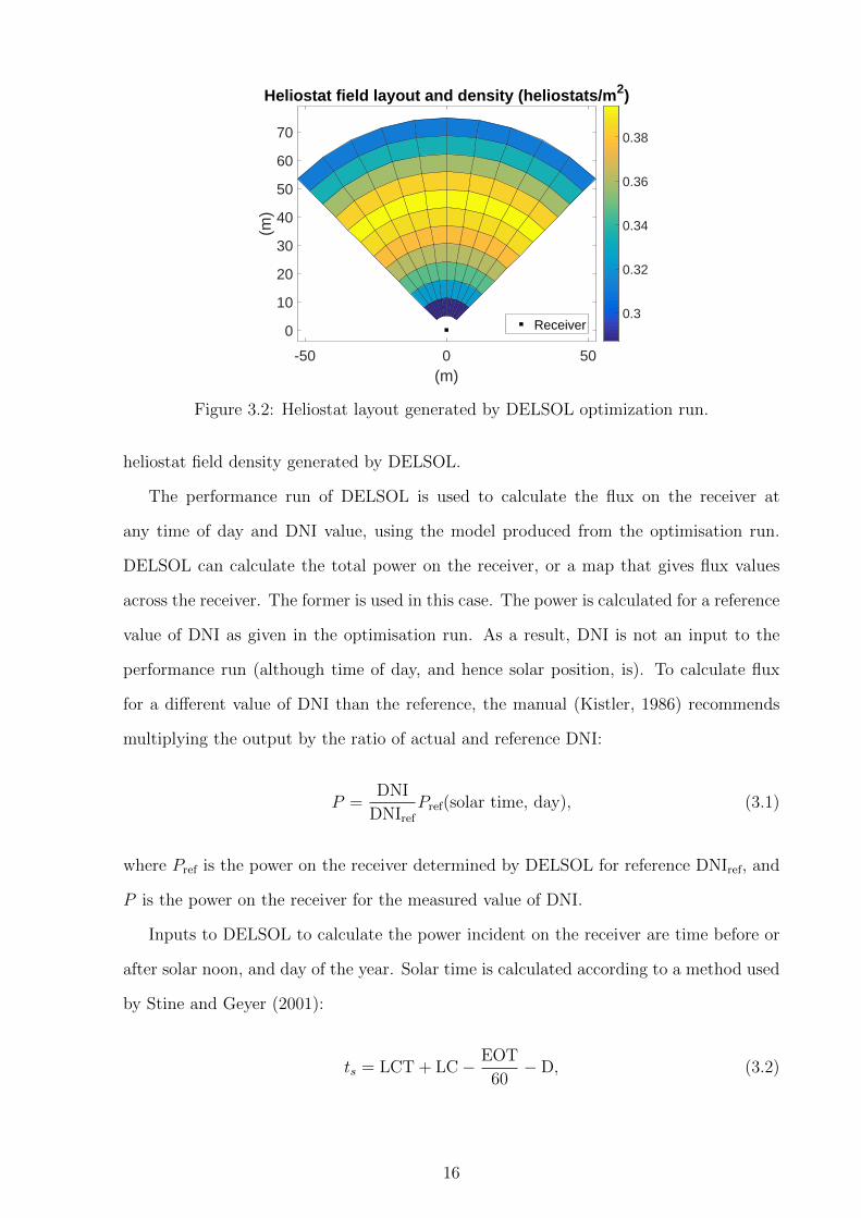
DELSOL does not place individual heliostats, but instead divides the field into zones
and generates heliostat density for each zone. See Figure 3.2 for a schematic showing the
15
-50 0 50(m)
0
10
20
30
40
50
60
70
(m)
Heliostat field layout and density (heliostats/m2)
0.3
0.32
0.34
0.36
0.38
Receiver
Figure 3.2: Heliostat layout generated by DELSOL optimization run.
heliostat field density generated by DELSOL.
The performance run of DELSOL is used to calculate the flux on the receiver at
any time of day and DNI value, using the model produced from the optimisation run.
DELSOL can calculate the total power on the receiver, or a map that gives flux values
across the receiver. The former is used in this case. The power is calculated for a reference
value of DNI as given in the optimisation run. As a result, DNI is not an input to the
performance run (although time of day, and hence solar position, is). To calculate flux
for a different value of DNI than the reference, the manual (Kistler, 1986) recommends
multiplying the output by the ratio of actual and reference DNI:
P =DNI
DNIref
Pref(solar time, day), (3.1)
where Pref is the power on the receiver determined by DELSOL for reference DNIref, and
P is the power on the receiver for the measured value of DNI.
Inputs to DELSOL to calculate the power incident on the receiver are time before or
after solar noon, and day of the year. Solar time is calculated according to a method used
by Stine and Geyer (2001):
ts = LCT + LC− EOT
60−D, (3.2)
16

where ts is the solar time and LCT is the local time in decimal 24 hour format. LC is a
longitude correction (in hours):
LC =λ− λTZM
15, (3.3)
where λ = 152.276 is the local longitude and λTZM = 150 is the longitude of the meridian
for the timezone. EOT is the equation of time (Lamm, 1981), calculated in minutes as:
EOT = 605∑i=0
(Ai cos
(360dleap365.26
)+Bi sin
(360dleap365.26
)), (3.4)
where dleap is the count of the day in the leap year cycle (starting with 1 on January 1 of
a leap year, and 1461 on December 31 of the fourth year); and the coefficients Ai and Bi
are given by the following lists:
A = 10−4 × 2.0870, 92.869,−522.58,−13.077,−21.867,−1.5100, (3.5)
B = 10−4 × 0,−1222.9,−1569.8,−51.602,−29.823,−2.3463. (3.6)
The day of the year is calculated by counting the days of the year and adding 172
days to convert to the equivalent day in the Northern Hemisphere.
Input files for DELSOL are given in Appendix B.
3.2 Receiver heat transfer and thermal energy stor-
age
The aim of the receiver model is to estimate the energy absorbed by the heat transfer
fluid, and thus the amount of fluid entering TES. This gives an estimate of the available
sodium in storage, ensuring the CSP plant has sufficient sodium to generate power. Since
the power block dynamics are decoupled from the receiver dynamics, the dynamics of this
model are ignored for simplicity.
The receiver is a tubular receiver design. Such receivers are made up of panels of small
tubes that run from the bottom to the top of the receiver, connected at either end by
a header pipe. Fluid flows in the same direction in each tube in the same panel. These
17

tubes act like fins, increasing heat transfer from pipe to HTF by increasing surface area
(Ho and Iverson, 2014). This receiver will be modelled as a single flat panel.
Sodium is assumed to enter the receiver at 270C and leave the receiver at 560C,
which are operating temperatures for the 1.1MWth Gemalong solar project (Vast Solar,
2016). In practise, a controller would be used to vary the flow rate of liquid sodium to
maintain the output temperature as DNI and flux on the receiver varies (Luo et al., 2016).
For this model, such a controller and receiver dynamics are ignored, but rather the flow
rate is calculated using a steady state model relating total power absorbed by the receiver
to the flow rate, assuming constant inlet and outlet temperatures:
fsod =Pabsorbed
cp∆T, (3.7)
where fsod is the flow rate of liquid sodium in kg/s, Pabsorbed is the power absorbed by the
fluid in the receiver in kW, cp is the specific heat capacity of liquid sodium in kJ/kg/K,
and ∆T = 560− 270 is the temperature difference in K.
The power absorbed by the heat transfer fluid in the receiver is determined by cal-
culating losses from the incident power. These losses are also calculated by DELSOL,
which accounts for both loss due to reflection at the receiver and losses due to radiation
and convection. The processes used to determine these are described by Kistler (1986).
Hence, the power absorbed by the heat transfer fluid in the receiver is given by:
Pabsorbed = Ptotal − Preflected − Prad/conv, (3.8)
where Ptotal is the gross power from concentrated sunlight at the receiver, Preflected accounts
for power lost due to reflection, and Prad/conv accounts for power lost due to radiation and
convection.
The TES system is a two-tank system, which has a hot fluid storage tank and a cold
fluid storage tank. The cold fluid storage tank is not modelled, as only the amount of
fluid in the hot storage tank is relevant to modelling the power output. It is assumed that
there is enough fluid in the cold tank to enable the plant to continue operating.
The hot tank is modelled as a constant temperature reservoir of liquid sodium. Losses
18

Figure 3.3: Schematic of power block showing liquid sodium flow as orange lines,steam/water flow as black lines, and cooling water flow as blue lines.
between the receiver and tank are ignored, so the liquid sodium is assumed to be at 560C.
Hence, power available in the TES can be quantified by the amount of liquid sodium in
the tank. This is determined by integrating the net flow of sodium into the tank:
msod =
∫ t1
t0
fin − foutdt, (3.9)
where fin is the flow rate in, determined as above, and fout is the mass flow rate out,
determined by the requirements of the power cycle.
3.3 Power block
The purpose of the power cycle model is to model the power production of the CSP plant.
The model must provide realistic dynamics of the power cycle as heat input is varied but
be simple enough to run quickly. The power cycle of the plant is a Rankine cycle, using
water/steam as the working fluid. The heat transfer fluid of the plant, liquid sodium, is
used as the heat input to the cycle, through a set of heat exchangers that heat the water
to steam. An infinite reservoir of cold water is assumed to feed the condenser, which cools
the steam to liquid. See Figure 3.3 for a schematic of the power block.
The model is adapted from van Putten and Colonna (2007), who developed a tran-
19

sient model of a 600kW Rankine cycle powered by combustion gasses. Some simplifying
assumptions are made here, so that it behaves more like a quasi-steady model. In par-
ticular, pressure drop through the heat exchangers due to friction losses are ignored, as
is mass accumulation in general. Hence, the flow rate of steam and feedwater are always
equal, although the rate is able to vary as the ratio of high to low pressure varies. The low
pressure is considered fixed and does not vary over time, but the high pressure varies. As
a result, there are only two inputs to the model, the flow rate of liquid sodium which pro-
vides heat in, and the flow rate of the cooling water which provides heat out. The sodium
flow rate is used as the control input in the control simulations described in Chapter 4.
The cooling water flow rate is varied to maintain a set point of enthalpy at the exit of the
condenser. Heat accumulation in the turbine and pump are also ignored.
Steam and water thermodynamic properties are calculated using the IF97 model in
FluidProp (Asimptote, 2016). Sodium thermodynamic properties are determined using
relations from Boerema et al. (2012).
3.3.1 Heat exchangers
The power cycle has a total of four shell and tube heat exchangers. Three are used for
heating the fluid: a preheater which brings water close to the saturation point; a boiler
where phase change occurs; and a superheater which adds further heat to bring the steam
above the saturation point. For these three, sodium is the heat source. The fourth heat
exchanger is the condenser, where phase change occurs to convert the vapour output of
the turbine to saturated liquid input to the pump. Each heat exchanger is modelled as
a set of coupled differential equations governing the change in state of both hot and cold
fluids, and the change in wall temperature separating the fluids. The van Putten and
Colonna (2007) model uses density and internal energy as the states for their differential
equations:
dρLdt
=1
V(fE − fL), (3.10)
duLdt
=1
ρV
(fEhE − fLhL + Q− uV dρL
dt
), (3.11)
20

where ρ represents density, V represents volume, f represents mass flow rate, u represents
internal energy, Q represents heat transfer flow rate, and subscripts E and L represent
properties corresponding to entering and leaving fluid respectively.
Since flow rate is constant through the heat exchangers, change in density is ignored.
Hence, the equations for each heat exchanger are:
duCdt
=1
ρCVC
(fC (hCE − hCL) + QC
), (3.12)
duHdt
=1
ρHVH
(fH (hHE − hHL) + QH
), (3.13)
dTwdt
=−(QH + QC)
mwCp,w, (3.14)
where subscript C refers to cold fluid and subscript H refers to hot fluid, mw is the mass
of the wall, and Cp,w is the specific heat capacity of the wall.
Heat transfer Q is given by:
Q = UA∆T, (3.15)
where U is the heat transfer coefficient, A is the surface area of the heat exchanger,
and ∆T is the temperature difference. Heat transfer coefficient for each heat exchanger
stage depends on whether the fluid is in the shell or the tube of the shell and tube heat
exchanger, and whether there is phase change, as well as whether it is from vapour to
liquid or liquid to vapour. These are given as (Colonna and van Putten, 2007):
U =
KCf0.6 for a single phase fluid in the shell,
KCf0.8 for a single phase fluid in the tube,
KT exp(
P43.45
)for boiling fluid,
KCT0.9sat for condensing fluid,
(3.16)
where KC represents a turbulent convection factor, KT represents Thom’s factor for nu-
cleate boiling, and Tsat represents the saturation temperature of water/steam.
21

3.3.2 Turbine
The turbine is modelled by a set of algebraic equations. The pressure ratio of the flow in
and out of the turbine is governed by Stodola’s ellipse (van Putten and Colonna, 2007):
f =
√√√√KfPEρE
(1−
(PLPE
)2), (3.17)
where Kf is an empirical flow factor, and P represents pressure. When entry and exit
conditions are known, this equation governs the flow rate of steam through the turbine.
The power output from the turbine is given by:
W = f(hE − hL), (3.18)
Enthalpy at the turbine outlet is a function of the isentropic efficiency:
hL = hE − (hE − his)ηis, (3.19)
where his is the enthalpy at the turbine outlet assuming an isentropic process, and ηis is
given by (van Putten and Colonna, 2007):
ηis = 4Ke0vBvF
(cosα− vB
vF
), (3.20)
where Ke0 is an efficiency parameter for the turbine, α is the angle of approach of the
blade relative to steam flow, and vBvF
is the ratio of rotor velocity to absolute flow velocity,
given by:
vBvF
=Kv0n√hE − his
, (3.21)
where Kv0 is a proportionality parameter for the turbine, and n is the rotational speed
of the turbine in rotations per second. Rotational speed n is assumed to be constant, as
the generator is connected to the grid. Generator losses are ignored.
22

3.3.3 Pump
The pump equations are used to determine the power input required to compress the fluid
from low to high pressure, and to determine the outlet conditions of the pump. Power
consumed by the pump is given by the equation (van Putten and Colonna, 2007):
Wpump =∆Pf
ηρ, (3.22)
where ∆P is the difference between high and low pressures, f is the flow rate of water
through the pump, η is the pump efficiency, and ρ is the average density through the
pump, approximated by:
ρ =ρE + ρL
2. (3.23)
The pump efficiency is given by (van Putten and Colonna, 2007):
η = ηD
1−
(1− V
VD
n
nD
)2 , (3.24)
where subscript D refers to design parameters, V is the volume flow rate through pump,
and n is the pump speed in rps. Pump speed and volume flow rate are related by the
following equation, which is solved to find the pump speed n (van Putten and Colonna,
2007):
V =− bngDD−√
b2n2
g2D2D
+ 4aHgD4
D− 4acn2
g2D2D
2agD4
D
, (3.25)
where DD represents pump impeller diameter, H = ∆P/ρg represents pump head for
current conditions, g is gravitational acceleration, and a, b, and c are coefficients found
by solving the following set of linear equations (van Putten and Colonna, 2007):
gHD
n2DD
2D
= a
(VD
nDD3D
)2
+ b
(VD
nDD3D
)+ c, (3.26)
0 = a
(V0
nDD3D
)2
+ b
(V0
nDD3D
)+ c, (3.27)
gH0
n2DD
2D
= c, (3.28)
23

where H0 represents pump head at zero flow and V0 represents volume flow at zero head.
3.3.4 Simulating the power cycle
The whole power cycle model consists of differential-algebraic equations. The heat ex-
changers are modelled by differential equations, and the turbomachinery are modelled
by algebraic equations. The heat exchanger states are solved by numerically integrating
using Matlab’s ode23s solver for stiff ODE systems. At the beginning of each step of the
solver, the algebraic equations are evaluated to give inlet conditions for the preheater and
condenser.
The parameters used with the models are taken from ? and shown in Tables 3.2 and
3.3. Figure 3.4 shows a simulation of the power cycle for a step change in liquid sodium
input from 11 kg/s to 13 kg/s.
3.4 Photovoltaic modules
The purpose of the photovoltaic (PV) array model is to model the power output of the PV
array during the day under varying solar irradiance and ambient conditions. The model
should take into account solar availability and all necessary ambient conditions (such as
wind speed and temperature) and provide power output of the array.
PV modules are sensitive to both direct and diffuse irradiance, so the global horizontal
irradiance (GHI) is used as a measure of irradiance on a PV module. The surfaces of the
solar panels which make up the PV array are assumed to be not inclined, so the direct
measurement of GHI can be used without modification or further calculations.
Zhou et al. (2007) provide a simple model of photovoltaic modules that can be used
for any module and determined from manufacturer specifications and some simple tests.
The model gives a way to determine maximum power available from the PV module and
is dependent on irradiance on the surface of the module, and cell temperature.
PV modules are characterised by an I-V curve which specifies the current for a given
operating voltage, as shown in Figure 3.5. The extreme values are short circuit current
corresponding to zero voltage, and open circuit voltage corresponding to zero current.
Maximum power is obtained at the knee of the curve, where I ·V is at a maximum (this is
24

0 5 10 15Time (min)
600
650
700
750
Pow
er (
kW)
Power cycle power output
0 5 10 15Time (min)
27
28
29
30
Pre
ssur
e (b
ar)
High pressure
(a)
0 5 10 15Time (min)
1.5
1.55
1.6
1.65
Flo
w r
ate
(kg/
s)
Steam/water flow rate
0 5 10 15Time (min)
18.5
19
19.5
20
20.5
Flo
w r
ate
(kg/
s)
Cooling water flow rate
(b)
0 5 10 15Time (min)
200
300
400
Tem
pera
ture
(o C
) Water/steam temperatures (high)
economiserboilersuperheater
0 5 10 15Time (min)
80
100
120
Tem
pera
ture
(o C
) Water/steam temperatures (low)
turbinecondenserpump
(c)
0 5 10 15Time (min)
250
300
350
400
450
500
550
Tem
pera
ture
(o C
)
Sodium temperatures (low)
economiserboilersuperheater
(d)
Figure 3.4: Power cycle response to step change in sodium flow rate from 11kg/s to13kg/s at time t = 0. (a) Power output; (b) working fluid and cooling fluid flow rates;(c) steam/water temperatures; (d) sodium temperatures.
Figure 3.5: Characteristic current-voltage curve of a photovoltaic module.
25

Table 3.2: Parameters used for heat exchanger modelling (van Putten and Colonna, 2007).
Preheater
Number of tubes 608Outer diameter of tubes 0.02 m
Length of tubes 3 mThickness of tubes 2.6E-03
Heat capacity of metal, Cp,w 0.5 kJ/kg KDensity of metal, ρw 7500 kg/m3
Volume of shell 1.7 m3
Turbulent convection factor, hot side, Kc,H 1.2E-02Turbulent convection factor, cold side, Kc,C 0.914
Boiler
Number of tubes 82Outer diameter of tubes 0.0635 m
Length of tubes 4.6 mThickness of tubes 5E-03
Heat capacity of metal, Cp,w 0.5 kJ/kg KDensity of metal, ρw 7500 kg/m3
Volume of shell 3.6 m3
Turbulent convection factor, hot side, Kc,H 3.57E-02Thom’s factor for nucleate boiling, KT 5.31
Superheater
Number of tubes 181Outer diameter of tubes 0.038 m
Length of tubes 3 mThickness of tubes 3.2E-03
Heat capacity of metal, Cp,w 0.5 kJ/kg KDensity of metal, ρw 7500 kg/m3
Volume of shell 1.93 m3
Turbulent convection factor, hot side, Kc,H 6.35E-03Turbulent convection factor, cold side, Kc,C 0.777
Condenser
Number of tubes 514Outer diameter of tubes 0.02 m
Length of tubes 4.88 mThickness of tubes 1.6E-03
Heat capacity of metal, Cp,w 0.5 kJ/kg KDensity of metal, ρw 7500 kg/m3
Volume of shell 2.16 m3
Condensing coefficient factor, hot side, Kc,H 0.087Turbulent coefficient factor, cold side, Kc,C 0.126
26

Table 3.3: Parameters used for turbomachinery modelling (van Putten and Colonna,2007).
Feedwater pump
Pump design head, HD 288.26 m
Pump design volume flow, VD 1.5724E-03 m3/sPump design efficiency, ηD 0.65
Pump design rotational speed, nD 58.33 rpsPump design impeller diameter, DD 100E-03 m
Pump volume flow at zero head, V0 2E-03 m3/sPump head at zero flow, H0 600 m
Turbine
Flow coefficient, Kf 9.01E-02 m2
Velocity parameter, Kv0 0.54 mEfficiency parameter, Ke0 0.7
Approach angle, α 0.3Turbine speed, 23 rps
shown as a yellow rectangle in Figure 3.5). The difference between this and the theoretical
maximum obtained from the open circuit voltage and the short circuit current (the red
rectangle in Figure 3.5) is known as the fill factor. Hence, maximum power available from
the module can be calculated from the fill factor, open circuit voltage and short circuit
current:
Pmax = FF · Isc · Voc, (3.29)
where Pmax is the maximum deliverable power, FF is the fill factor, Isc is the short circuit
current, and Voc is the open circuit voltage. A Maximum Power Point Tracking (MPPT)
controller is used to ensure the module is always operating at its maximum power output.
Short circuit voltage is primarily affected by changes in irradiance, so is governed by
the following equation (Zhou et al., 2007):
Isc = Isc0
(G
G0
)α, (3.30)
where Isc0 (A) is some reference short circuit current at irradiance G0 (W/m2), G is the
present solar irradiance (W/m2), and α accounts for non-linear effects.
Open circuit voltage depends on both irradiance and cell temperature (Zhou et al.,
27

Table 3.4: Parameters for photovoltaic cell model (Zhou et al., 2007).
α β γ n Rs(Ω)
1.21 0.058 1.15 1.17 0.012
2007):
Voc =Voc0
1 + β ln(G0
G
) (T0
T
)γ, (3.31)
where Voc0 is a reference open circuit voltage for irradiance value G0 and reference tem-
perature T0 (K), T is current cell temperature (K), β is a parameter related to the PV
module, and γ accounts for non-linear effects.
Fill factor is given by (Zhou et al., 2007):
FF = FF0
(1− Rs
Voc/Isc
), (3.32)
where Rs is series resistance of the module, and FF0 is given by:
FF0 =voc − ln (voc + 0.72)
1 + voc, (3.33)
and voc is given by:
VocnKT/q
, (3.34)
where 1 ≤ n ≤ 2 is an ideality factor for the PV module, K = 1.38 × 10⁻²³ J/K is the
Stefan-Boltzmann constant, T (K) is the module temperature, and q = 1.6 × 10⁻¹⁹ C is
the magnitude of charge of an electron.
Zhou et al. (2007) outlined procedures to determine the PV module parameters for
this model. They determined the parameters for a monocrystalline module, which are
used in this report also, and given in Table 3.4.
The PV module short circuit current, and open circuit voltage reference values are
taken from BP Solar (2003) and given in Table 3.5. These are given for a nominal 80W
module.
The cell temperature is determined using a transient model developed by Jones and
Underwood (2001). This model accounts for radiative heat transferqlw, heat transfer from
solar irradiance qsw, heat transfer due to convection qconv and heat transfer from power
28

Table 3.5: Photovoltaic cell reference values (BP Solar, 2003).
Voc0 [V] Isc0 [A] G0 [W/m2] T0 [C]
22.1 5.0 1000 25
out Pout:
CmoduledT
dt= qlw + qsw + qconv − Pout. (3.35)
Details of the calculation of the heat transfer model are given in Appendix A.
This model is a steady state model which does not take into account PV module
dynamics. However, the response time of PV modules is in the order of milliseconds
(cai Dai et al., 1991), whereas the time-scale for the CSP plant model is in the order of
minutes, hence the dynamics of PV can be ignored.
The total power output of a PV array depends on the number of modules connected
in series and in parallel. Connecting modules in series scales up voltage, and connecting
modules in parallel scales up current. Hence, it is ideal to connect both in series and in
parallel to maximise the power from the same number of modules. Assuming that each
module has the same performance characteristics, total power of the array is given by:
PA = Np ·Ns · PM , (3.36)
where PA represents the total power of the array, PM represents individual module power,
and Np and Ns represent number of modules connected in parallel and series respectively.
Each individual panel gives a nominal 80W output. For a power output of 300kW, a total
of 3750 panels are used in a 50 × 75 panel array. In practise, the array may be made up
of a smaller number of panels with higher nominal power output.
Simulated energy production for an overcast day is given in Figure 3.6.
3.5 Battery model
The purpose of the battery model is to show battery dynamics as state of charge (SOC)
and load vary. The battery model should keep track of available power in the battery, as
well as the dynamics of its response to varying load.
29

Figure 3.6: Photovoltaic panel simulation.
The model developed by Chen and Rincon-Mora (2006) is used. This model is devel-
oped for a 850mAh lithium ion cell. To give a suitable battery bank for the photovoltaic
application, many cells will be lumped into one model. As with photovoltaic modules, it
is assumed that connecting batteries in series will multiply the voltage of the individual
batteries, and connecting the batteries in parallel will multiply the current.
The electrical circuit model is given in Figure 3.7. The battery lifetime circuit models
the state of charge of the battery, represented by VSOC, a value between 0 and 1 which
Figure 3.7: Chen and Rincon-Mora (2006) battery circuit model showing battery lifetimecircuit modelling state of charge, and voltage-current characteristics circuit. Reprintedfrom Fares and Webber (2015).
30

represents charge remaining in the battery. This model accounts for both charge and
discharge. Applying a positive current depletes the battery, and applying a negative
current charges the battery. The voltage-current characteristics circuit models the battery
voltage for varying current and state of charge. All parameters are variable with state of
charge.
The equations of the dynamics are given by (Fares and Webber, 2015):
VSOC = − Ibatt
Ccapacity
, (3.37)
Vtransient,S =Ibatt
Ctransient,S
− Vtransient,S
Rtransient,SCtransient,S
, (3.38)
Vtransient,L =Ibatt
Ctransient,L
− Vtransient,L
Rtransient,LCtransient,L
, (3.39)
and battery output voltage is given by:
Vbatt = VOC − IbattRseries − Vtransient,S − Vtransient,L. (3.40)
Components are all functions of the SOC, as given by Chen and Rincon-Mora (2006):
Ccapacity = 3060, (3.41)
VOC = −1.031e−35VSOC + 3.685 + 0.2156VSOC − 0.1178V 2SOC + 0.3201VSOC, (3.42)
Rseries = 0.1562e−24.37VSOC + 0.07446, (3.43)
Rtransient,S = 0.308e−29.14VSOC + 0.04669, (3.44)
Ctransient,S = −752.9e−13.51VSOC + 703.6, (3.45)
Rtransient,L = 6.603e−155.2VSOC + 0.04984, (3.46)
Ctransient,L = −6056e−27.12VSOC + 4475. (3.47)
All capacitance values are given in F, voltage in V, and resistance in Ω.
To model power output, current will be varied to meet a required load, such that the
power output remains constant (or at the desired value) even as SOC and thus battery
voltage varies:
Ibatt =Pdesired
Vbatt
. (3.48)
31

Battery performance is shown in the simulations Chapter 4.
32

Chapter 4
Control methodology and results
This chapter presents the methodology used for the control simulations, the contribution
of this work. This includes a brief overview of model predictive control and the forecast
methods used to generate the DNI predictions used here. Results are presented and
discussed.
4.1 Methodology
4.1.1 Model predictive control background
Model predictive control (MPC) is chosen as the control strategy for the power cycle as
it is able to take advantage of forecasts, and enables constraints on the inputs. MPC in
general is used to find the optimal control input to meet some criteria, or minimise some
cost function. The philosophy of MPC is to develop a schedule of inputs to minimise
the cost function over some time horizon, then implement the first step of the control
schedule, and repeat for the next timestep. Further detailed information about MPC can
be found in Wang (2009), but an overview of key features is given here.
MPC is used to determine an optimal control trajectory over a fixed time horizon, and
here is implemented in discrete time. The time window moves; at the beginning of each
timestep, the MPC problem is solved for the time window starting at that point. This
time window describes how far into the future the plant performance must be predicted.
MPC requires a suitable model of the plant under control. This plant gives a prediction
33

of its dynamic behaviour as a function of the measurements available at the start of the
time window and a proposed control schedule. A cost function is used to judge how
well the control schedule meets the objective. This cost function may also be subject
to constraints on the inputs or plant states. The optimal control schedule is found by
minimising this function.
At each timestep, once the MPC problem has been solved to find the optimal tra-
jectory, only the first step is implemented. The MPC process is then repeated for the
updated plant measurements available at the next timestep.
4.1.2 Power cycle control
The plant under control is the power block of the CSP plant. The control objective of this
simulation is to track a reference load in order to maintain a constant power output from
the combined plant. The reference power output for the CSP power block is determined
from the difference between the total hybrid plant desired output, and the power provided
by the photovoltaic array:
PCSP = Pdesired − PPV, (4.1)
An example of the hybrid, PV, and resulting desired CSP power curves curves is given in
Figure 4.1. Due to the presence of sudden drops in solar availability, there are large step
changes in the CSP output reference. Given the dynamics of the power cycle simulation
shown in Figure 3.4, it is unrealistic to achieve this with the CSP power cycle alone.
Hence, the battery system will be used to supply or absorb extra power to cover the
difference. Nevertheless, it is desirable to minimise the error of the power cycle load
tracking, so that the size of the batteries can also be minimised.
The cost function used to evaluate the control objective finds the difference between
CSP power output and the required output at the end of each timestep in the time horizon:
J(t) =n∑i=1
(Pdesired(t+ i∆t)− PCSP(t+ i∆t))2 , (4.2)
where n is the number of timesteps in the forecast horizon, Pdesired(t + i∆t) represents
the prediction of required power output at the ith timestep in the forecast horizon, and
34

10:30:00 11:00:00 11:30:00 12:00:00
Time (s)
0
100
200
300
400
500
600
700
800
900
Pow
er (
kW)
Combined and separate power outputs
TotalPV supplyCSP desired
Figure 4.1: Example of power output from PV array and resulting desired power outputfrom CSP.
PCSP(t+ i∆t) is the prediction of the power output of the CSP plant at the ith timestep
based on the simplified plant model. The desired load is a predicted value as solar irra-
diance and therefore PV power output is not known in advance. The forecasts of solar
availability are used to determine the desired load.
The power cycle model is linearised about the operating point at each MPC step to
provide a simplified model of the dynamics. The linearisation is based on a Taylor series
expansion of the state equations:
ˆx =∂f
∂x
∣∣∣∣x=xo,u=uo
· (x− xo) +∂f
∂u
∣∣∣∣x=xo,u=uo
(u− uo) + f(xo, uo) + h.o.t., (4.3)
where ∂f∂x
∣∣x=xo,u=uo
represents the Jacobian matrix of f(x, u) evaluated at the operating
point x = xo, u = uo, and h.o.t. represents higher order terms, which are ignored. The
linearisation is calculated numerically using a forward difference. The linearised state
equation is used to numerically integrate the output over the simulation step using the
Euler method (Hamming, 2012):
xk+1 = xk + δtˆx. (4.4)
35

The timestep used for the MPC is sufficiently large to cause numerical instability, so
this integration is performed several times over a smaller timestep δt (although ˆx is not
recalculated every time).
Constraints are placed on the sodium flow rate and step size. The flow rate is bounded
between 1 and 30 kg/s. The input is also bounded not to change more than 3 kg/s in any
timestep. This represents a constraint that the sodium cannot change instantaneously by
a large amount.
Power output required during the forecast period depends on the method of DNI
forecasting used. Solar availability forecasts are used with the PV array model to give
forecasts of PV power production, and thus forecast the required output of the CSP.
The MPC problem is solved by numerical minimisation using the MATLAB function
fmincon. This permits easy implementation of the described method and constraints.
After each MPC step, the first of the determined inputs is used in the (non-linearised)
power cycle simulation function to give the power output over the desired step.
4.1.3 Forecasts
Forecasts of DNI from Pidgeon (2014) are incorporated into this controller in order to
predict the power output of the PV array. Three different forecast models are used. First,
persistence or no forecast: in this method, a zero order hold is used on the previous known
value of DNI, so power output is constant over the forecast horizon. The second method
is using DNI predictions from the sky imager. The third method is the prescient model,
where the perfect knowledge of DNI is assumed. The measured values of DNI for the day
are used as prediction inputs.
Global horizontal irradiance (GHI) values are required to estimate the PV power
output. However, the forecast algorithm from Pidgeon (2014) only predicts DNI. Hence,
GHI is estimated with the following relation:
GHI = DHI + DNI cos(z), (4.5)
where DHI is the diffuse horizontal irradiance, and z is the solar zenith angle (refer to
Pidgeon (2014) for the calculation method). DHI measurements are available. A zero
36

order hold is used for the most recent measured value, allowing GHI to be calculated for
the forecast period. Since DHI is a small fraction of DNI, this should not impact the
predictions or control significantly.
Forecasts from Pidgeon (2014) are used. This algorithm combines a clear sky model to
predict clear sky DNI, and cloud vector tracking from ground-based sky images to predict
the cloud fraction blocking the sun. The cloud fraction is used to scale the clear sky DNI
estimate, as given by (Pidgeon, 2014):
Bt+∆t = Bclrt+∆t(1− C
ft+∆t), (4.6)
where Bt+∆t represents the prediction of DNI in W/m2 at time t+∆t, Bclrt+∆t represents the
clear sky DNI (W/m2), and Cft+∆t represents the cloud fraction. For further information,
see Pidgeon (2014). Examples of DNI forecasts for 5 and 10 minutes ahead are given in
Figure 4.2.
This method provides forecasts for horizons of 1 to 15 minutes, at 1 minute intervals.
However, for a forecast horizon of 1-3 minutes, the error of the forecasts from this method
are significantly greater than the error from persistence based forecasts (Pidgeon, 2014).
The forecast method has a high rate of false positives, as is evident in Figure 4.2. This is
exacerbated for a short forecast period, as the sky imaging software tends to erroneously
classify sun glare as clouds (Pidgeon, 2014). As a result, the first three minutes of forecast
use a persistence prediction instead of the forecasts from the sky imager. Examples of the
predicted DNI from each of the prediction methods is given in Figure 4.3. A noteworthy
feature is the lack of continuity between predictions. The sequential predictions, each
only a minute apart, show that successive DNI predictions are vastly different, with little
continuity of expected troughs.
4.2 Results of simulation
Two simulations are run for the following time periods: 8/11/2014, 10:30 AM to 11:30
AM, and 29/11/2014, 11:11 AM to 12:36 PM. These periods have been chosen as they are
times with significant ramp events, where cloud cover leads to rapidly changing DNI. This
37

10:30:00 10:45:00 11:00:00 11:15:00 11:30:00 11:45:00Time
0
100
200
300
400
500
600
700
800
900
1000
DN
I (W
/m2 )
DNI predictions for 8/11/14, 5 min forecast
ActualForecast
(a)
10:30:00 10:45:00 11:00:00 11:15:00 11:30:00 11:45:00Time
0
100
200
300
400
500
600
700
800
900
1000
DN
I (W
/m2 )
DNI predictions for 8/11/14, 10 min forecast
ActualForecast
(b)
11:30:00 12:00:00 12:30:00Time
0
200
400
600
800
1000
1200
DN
I (W
/m2 )
DNI predictions for 29/11/14, 5 min forecast
ActualForecast
(c)
11:30:00 12:00:00 12:30:00Time
0
200
400
600
800
1000
1200
DN
I (W
/m2 )
DNI predictions for 29/11/14, 10 min forecast
ActualForecast
(d)
Figure 4.2: DNI forecasts from Pidgeon (2014). (a) and (b) show 5 and 10 minuteforecasts respectively for 8/11/14, and (c) and (d) show 5 and 10 minute ahead forecastsfor 29/11/14.
38

12:00:00 12:05:00 12:10:00 12:15:00
Time
0
200
400
600
800
1000
DN
I (W
/m2 )
Forecast at 29-Nov-2014 11:58:00
PrescientPersistentPrediction
12:00:00 12:05:00 12:10:00 12:15:00
Time
0
200
400
600
800
1000
DN
I (W
/m2 )
Forecast at 29-Nov-2014 11:59:00
PrescientPersistentPrediction
12:00:00 12:05:00 12:10:00 12:15:00
Time
0
200
400
600
800
1000
DN
I (W
/m2 )
Forecast at 29-Nov-2014 12:00:00
PrescientPersistentPrediction
12:00:00 12:05:00 12:10:00 12:15:00
Time
0
200
400
600
800
1000
DN
I (W
/m2 )
Forecast at 29-Nov-2014 12:01:00
PrescientPersistentPrediction
Figure 4.3: Example of 15 minute horizon predictions from sequential measurements.This figure also shows forecasts using persistence and prescience.
causes large step changes in the CSP power reference curve. The predictions for 8/11/2014
tend to over-predict the DNI, whereas the 29/11/2014 data is much more conservative.
There is also a high rate of false positives for detecting cloud cover, particularly between
11:30 AM and 12:00 PM.
Two different forecast horizons are tested, 5 minutes and 10 minutes ahead forecasting.
Figures 4.4 and 4.5 show the power output of the hybrid plant for each simulation period
and both forecast horizons. These show the power output of the PV array, the CSP
plant, and the batteries for each forecast method. Note that a negative value in the
battery model indicates that excess power has been produced, and so the batteries are
charging instead of discharging. Tables 4.1 and 4.2 give the root mean squared error
(RMSE) of the CSP power output, given by:
RMSE =
√∑ni (Pdesired(i)− PCSP(i))2
n, (4.7)
where n is the number of timesteps in the simulation. The improvement in each forecast
39

Table 4.1: Summary of results, 8/11/14.
5 minute horizon 10 minute horizonMethod RMSE (kW) Improvement (%) RMSE (kW) Improvement (%)
Persistence 120 - 120 -Prediction 114 5.0 109 9.2Prescience 70 41.7 59 50.8
Table 4.2: Summary of results, 29/11/14.
5 minute horizon 10 minute horizonMethod RMSE (kW) Improvement (%) RMSE (kW) Improvement (%)
Persistence 151 - 151 -Prediction 141 v6.6 135 10.6Prescience 96 36.4 87 42.3
method relative to persistence is also given. This is calculated as follows:
Improvement =RMSEpersistent −RMSEprediction
RMSEpersistent
(4.8)
Tables 4.3 and 4.4 show the battery capacity required to supply the battery power
curve. Figures 4.6 and 4.7 show the state of charge of the battery over the simulation
period. These sizes are determined by finding the smallest number of cells connected in
parallel and series which are able to meet all extra power demand. This is determined
without requiring a certain state of charge at the end of the simulation, and assuming
that the batteries are full to begin with. Hence, they are not an indication of the size of
battery required for the hybrid plant overall, but only to enable the plant to meet the
load during the short time period of the simulation. Note that when the SOC is at 1, this
indicates that excess power generation is wasted, as the batteries are full. Hence, it is
most desirable that the plant over- and under-produces a comparable amount of power,
so that the battery is neither continuously depleted nor continuously full and unable to
store any more power.
4.3 Discussion
Due to the time dynamics of the power cycle, the CSP plant is unable to exactly meet
the desired power output curve. However, the controller which uses prescient forecasts of
40

10:30:00 11:00:00Time
0
200
400
600
800
1000
1200Ir
radi
ance
(W
/m2 )
GHI, 8/11/14
(a)
10:30:00 10:45:00 11:00:00 11:15:00Time
0
50
100
150
200
250
300
350
400
450
Pow
er (
kW)
PV plant output, 8/11/14
(b)
10:30:00 10:40:00 10:50:00 11:00:00 11:10:00 11:20:00Time
450
500
550
600
650
700
750
800
850
900
Pow
er (
kW)
CSP plant output, 8/11/14, horizon = 5 min
PrescientPersistentPredictionDesired
(c)
10:30:00 10:40:00 10:50:00 11:00:00 11:10:00 11:20:00Time
-400
-300
-200
-100
0
100
200
300
Pow
er (
kW)
Battery output, 8/11/14, horizon = 5 min
PrescientPersistentPrediction
(d)
10:30:00 10:40:00 10:50:00 11:00:00 11:10:00 11:20:00Time
450
500
550
600
650
700
750
800
850
900
Pow
er (
kW)
CSP plant output, 8/11/14, horizon = 10 min
PrescientPersistentPredictionDesired
(e)
10:30:00 10:40:00 10:50:00 11:00:00 11:10:00 11:20:00Time
-400
-300
-200
-100
0
100
200
300
Pow
er (
kW)
Battery output, 8/11/14, horizon = 10 min
PrescientPersistentPrediction
(f)
Figure 4.4: Simulation results for 8/11/14. (a) Shows the GHI measurement over thetime period, (b) shows the corresponding PV output, (c) and (e) show the CSP poweroutput and reference curves for the 5 and 10 minute forecast horizons respectively, and(d) and (f) show the battery power output for each period, reflecting the error betweenthe reference output and actual output of the CSP cycle.
41

11:30:00 12:00:00 12:30:00Time
0
200
400
600
800
1000
1200
1400Ir
radi
ance
(W
/m2 )
GHI, 29/11/14
(a)
11:30:00 12:00:00 12:30:00Time
0
100
200
300
400
500
600
Pow
er (
kW)
PV plant output, 29/11/14
(b)
11:30:00 12:00:00 12:30:00Time
300
400
500
600
700
800
900
Pow
er (
kW)
CSP plant output, 29/11/14, horizon = 5 min
PrescientPersistentPredictionDesired
(c)
11:30:00 12:00:00 12:30:00Time
-400
-300
-200
-100
0
100
200
300
400
Pow
er (
kW)
Battery output, 29/11/14, horizon = 5 min
PrescientPersistentPrediction
(d)
11:30:00 12:00:00 12:30:00Time
300
400
500
600
700
800
900
Pow
er (
kW)
CSP plant output, 29/11/14, horizon = 10 min
PrescientPersistentPredictionDesired
(e)
11:30:00 12:00:00 12:30:00Time
-400
-300
-200
-100
0
100
200
300
400
Pow
er (
kW)
Battery output, 29/11/14, horizon = 10 min
PrescientPersistentPrediction
(f)
Figure 4.5: Simulation results for 29/11/14. (a) Shows the GHI measurement over thetime period, (b) shows the corresponding PV output, (c) and (e) show the CSP poweroutput and reference curves for the 5 and 10 minute forecast horizons respectively, and(d) and (f) show the battery power output for each period, reflecting the error betweenthe reference output and actual output of the CSP cycle.
42

Table 4.3: Battery sizes, 8/11/14.
5 minute horizon 10 minute horizonMethod Capacity Improvement (%) Capacity Improvement (%)
Persistence 7.2 - 7.2 -Prediction 7.2 0 7.2 0Prescience 5.7 20 4.5 38
Table 4.4: Battery sizes, 29/11/14.
5 minute horizon 10 minute horizonMethod Capacity (kAh) Improvement (%) Capacity (kAh) Improvement (%)
Persistence 13.8 - 13.8 -Prediction 11.7 15.4 11.7 15.4Prescience 8.5 38.5 8.3 40.0
10:30:00 10:40:00 10:50:00 11:00:00 11:10:00 11:20:00 11:30:00Time (s)
0.3
0.4
0.5
0.6
0.7
0.8
0.9
1
1.1
Sta
te o
f cha
rge
Battery state of charge
(a) Persistence, 5 min
10:30:00 10:40:00 10:50:00 11:00:00 11:10:00 11:20:00 11:30:00Time (s)
0.2
0.3
0.4
0.5
0.6
0.7
0.8
0.9
1
1.1
Sta
te o
f cha
rge
Battery state of charge
(b) Predictions, 5 min
10:30:00 10:40:00 10:50:00 11:00:00 11:10:00 11:20:00 11:30:00Time (s)
0.2
0.3
0.4
0.5
0.6
0.7
0.8
0.9
1
1.1
Sta
te o
f cha
rge
Battery state of charge
(c) Prescience, 5 min
10:30:00 10:40:00 10:50:00 11:00:00 11:10:00 11:20:00 11:30:00Time (s)
0.3
0.4
0.5
0.6
0.7
0.8
0.9
1
1.1
Sta
te o
f cha
rge
Battery state of charge
(d) Persistence, 10 min
10:30:00 10:40:00 10:50:00 11:00:00 11:10:00 11:20:00 11:30:00Time (s)
0
0.2
0.4
0.6
0.8
1
1.2
Sta
te o
f cha
rge
Battery state of charge
(e) Predictions, 10 min
10:30:00 10:40:00 10:50:00 11:00:00 11:10:00 11:20:00 11:30:00Time (s)
0
0.2
0.4
0.6
0.8
1
1.2
Sta
te o
f cha
rge
Battery state of charge
(f) Prescience, 10 min
Figure 4.6: Battery state of charge for 8/11/14 simulations.
43

11:00:00 11:30:00 12:00:00 12:30:00 13:00:00Time (s)
0
0.2
0.4
0.6
0.8
1
1.2
Sta
te o
f cha
rge
Battery state of charge
(a) Persistence, 5 min
11:00:00 11:30:00 12:00:00 12:30:00 13:00:00Time (s)
0
0.2
0.4
0.6
0.8
1
1.2
Sta
te o
f cha
rge
Battery state of charge
(b) Predictions, 5 min
11:00:00 11:30:00 12:00:00 12:30:00 13:00:00Time (s)
0.2
0.3
0.4
0.5
0.6
0.7
0.8
0.9
1
1.1
Sta
te o
f cha
rge
Battery state of charge
(c) Prescience, 5 min
11:00:00 11:30:00 12:00:00 12:30:00 13:00:00Time (s)
0
0.2
0.4
0.6
0.8
1
1.2
Sta
te o
f cha
rge
Battery state of charge
(d) Persistence, 10 min
11:00:00 11:30:00 12:00:00 12:30:00 13:00:00Time (s)
0
0.2
0.4
0.6
0.8
1
1.2
Sta
te o
f cha
rge
Battery state of charge
(e) Predictions, 10 min
11:00:00 11:30:00 12:00:00 12:30:00 13:00:00Time (s)
0.4
0.5
0.6
0.7
0.8
0.9
1
1.1
Sta
te o
f cha
rge
Battery state of charge
(f) Prescience, 10 min
Figure 4.7: Battery state of charge for 29/11/14 simulations.
GHI is best able to track the curve with least lag or overshoot. By contrast, the persistent
model lags, since this method cannot anticipate sharp rises or drops in the required power.
As a result, this method tends to lead to overshoot: when the desired power level has
dropped, the output continues to rise.
The use of predictions does not give much improvement over the persistence method.
This is particularly evident in the 8/11/14 simulation, where the prediction method has
a very similar shape to the persistence method, with slightly lower peaks. There is no
reduction in battery size requirements. The shapes of both the prediction and persistence
curves are also quite similar in the 29/11/14 simulation. In both, the prediction method
suffers from the same tendency to lag.
Several factors contribute to this. Firstly, the first three minutes of the forecast are
persistence values, so the desired power output in the first three minutes of the time
window are also the same. Secondly, as already observed in Figure 4.2, the accuracy of
the prediction method is poor. The method is able to detect ramp periods, but its troughs
rarely coincide with the troughs in the measured data. The predictions also contain false
positives, where clouds are detected when there are none.
The other main concern is the lack of forecast continuity, as observed in Figure 4.3.
Although a trough may be predicted to occur 5 minutes ahead in one timestep, it is rarely
44

the case that the 4 minute ahead prediction made at the next timestep also shows a trough.
This means that at each timestep, the controller is preparing for a vastly different scenario,
unlike the prescient controller. With perfect knowledge, each successive prediction looks
like the previous prediction shifted forward by one minute. As a result, the optimal control
trajectory from one minute to the next does not vary much.
From the available prediction data, it cannot be determined whether the lack of conti-
nuity is an inherent problem of the prediction algorithm, or whether it could be improved
by simply increasing the sample time of measurements and predictions. Both avenues to
improve the prediction method could be explored.
Despite the inaccuracies in the prediction, the prediction method is able to decrease
the error in CSP power output tracking, albeit much less significantly than the prescient
model (see Tables 4.1 and 4.2). The prescient model also reduces the battery capacity
required to maintain the power output over the simulation period. The battery capacity
required when using DNI predictions is only improved for the 29/11/14 simulation. This
is likely a result of the conservative DNI predictions on this day, causing the CSP power
block to produce excess power. The battery state of charge plots in Figure 4.7 show that
for the predictions method, the battery SOC is higher than for the persistence method.
There are minor differences in the performance of simulations for a five minute forecast
horizon and a ten minute forecast horizon. While the error of the persistence method
does not change between the two simulations, both the predictions and prescient methods
show a slight decrease in error for the 10 minute forecast horizon. This demonstrates
that the state at 10 minutes ahead has some impact on choices made at the current time,
and indicates that longer forecast horizons improve error tracking when there are some
predictions available. For the prediction model, this improvement may also be explained
in that more of the values are actual predictions, not persistence data.
Generally it can be seen that a small improvement in performance is given by the use of
predictions. A significant performance improvement is possible with perfect predictions,
which indicates that improving the accuracy of the prediction method can improve the
load tracking ability of the power cycle in the context of this hybrid plant.
45

Chapter 5
Conclusion
The purpose of this thesis has been to investigate the value of short term (up to 15
minute) forecasts of solar availability in the operation of a combined photovoltaic (PV)
and concentrating solar thermal (CSP) power plant with both battery and thermal energy
(TES) storage. The forecast method led to small improvements in the load tracking ability
of the hybrid plant. However, the increase was small compared to the use of perfect
knowledge. Nevertheless, this work gives insights on what aspects of solar availability
forecasting can be improved in order to work better for this application.
Three methods of predicting solar availability were compared: a persistence model
corresponding to no predictions; a prescient model corresponding to perfect predictions;
and the causal prediction method developed by Pidgeon (2014) which generates 1-15
minute forecasts of direct normal irradiance (DNI). These forecasts were used to predict
the power output of the photovoltaic array, in order to predict the power output required
by the CSP system to maintain a constant output from the combined hybrid plant. Model
predictive control was used to control the power block of the CSP system in order to meet
the predicted load.
The prescient model led to a 35-50% reduction in the RMSE between the desired load
and actual power cycle output, compared to the model with no predictions. By contrast,
the prediction method from Pidgeon (2014) gave between a 5-10% reduction in the RMSE
compared to no predictions. Better load tracking performance can also reduce the battery
storage capacity required of the plant, which is a significant cost in hybrid plant designs
(Petrollese and Cocco, 2016). The prescient model led to a 20-40% decrease in battery size
46

required for the simulation period compared to the persistence model. The predictions
gave between 0-15% decrease in required battery capacity.
As a result, it is evident that accurate predictions can lead to improvements in plant
performance and a decrease in costs related to battery storage, although further investi-
gations into the sizing of the hybrid plant and its components should be undertaken. In
particular, the prescient predictions give an indication of the maximum improvements pos-
sible. However, the causal predictions did not match this performance. This was largely
due to the low accuracy of the prediction data. For MPC, the continuity of the forecasts
is important. It is ideal if the predicted DNI for two successive time windows have similar
shape, as this would indicate consistency in the prediction method over each time step. It
is believed that a prediction algorithm that factors in continuity of its predictions would
lead to greater accuracy, and thus better performance in an MPC controller.
Further work involving forecasts could combine long-term (1-3 days ahead) forecasts
to develop schedules of optimal power generation, and assess the usefulness of short-term
forecasts in meeting these load curves. A more complex model could take into account
factors such as electricity market behaviour, peak load, and solar resource availability
over an entire day of simulation. This would enable exploration of optimisation methods
using scheduling to maximise profit, or optimise the sizes of each component of the hybrid
plant; optimisation with more complex cost functions than have been considered here.
47

References
Angelini, G., Lucchini, A., and Manzolini, G. (2014). Comparison of thermocline molten
salt storage performances to commercial two-tank configuration. Energy Procedia,
49:694 – 704.
Asimptote (2016). Fluidprop. Software.
Boerema, N., Morrison, G., Taylor, R., and Rosengarten, G. (2012). Liquid sodium versus
hitec as a heat transfer fluid in solar thermal central receiver systems. Solar Energy,
86(9):2293 – 2305.
BP Solar (2003). BP 585 85-Watt High-Efficiency Monocrystalline Photovoltaic Module.
cai Dai, G., hai Miao, Q., zao Ren, Z., xun Zheng, Z., and lei Ma, H. (1991). Transient
behaviour of short-circuit current and open-circuit voltage in a-si:h solar cells. Solar
Cells, 31(3):279 – 281.
Chen, M. and Rincon-Mora, G. A. (2006). Accurate electrical battery model capable of
predicting runtime and I-V performance. IEEE Transactions on Energy Conversion,
21(2):504–511.
Chen, R., Sun, H., Guo, Q., Li, Z., Deng, T., Wu, W., and Zhang, B. (2015). Reduc-
ing generation uncertainty by integrating csp with wind power: An adaptive robust
optimization-based analysis. IEEE Transactions on Sustainable Energy, 6(2):583–594.
Colonna, P. and van Putten, H. (2007). Dynamic modeling of steam power cycles: Part I
– modeling paradigm and validation. Applied Thermal Engineering, 27(23):467 – 480.
Denholm, P. and Hand, M. (2011). Grid flexibility and storage required to achieve very
high penetration of variable renewable electricity. Energy Policy, 39(3):1817 – 1830.
48

Faille, D., Liu, S., Z.Wang, and Yang, Z. (2014). Control design model for a solar tower
plant. Energy Procedia, 49:2080 – 2089. Proceedings of the SolarPACES 2013 Interna-
tional Conference.
Fares, R. L. and Webber, M. E. (2015). Combining a dynamic battery model with
high-resolution smart grid data to assess microgrid islanding lifetime. Applied Energy,
137:482 – 489.
Garcıa, I. L., Alvarez, J. L., and Blanco, D. (2011). Performance model for parabolic
trough solar thermal power plants with thermal storage: Comparison to operating
plant data. Solar Energy, 85(10):2443 – 2460.
Garcia, P., Ferriere, A., and Bezian, J.-J. (2008). Codes for solar flux calculation dedicated
to central receiver system applications: A comparative review. Solar Energy, 82(3):189
– 197.
Hamming, R. (2012). Numerical Methods for Scientists and Engineers. Newburyport :
Dover Publications, Newburyport.
Ho, C. K. and Iverson, B. D. (2014). Review of high-temperature central receiver designs
for concentrating solar power. Renewable and Sustainable Energy Reviews, 29:835 –
846.
Jianfeng, L., Jing, D., and Jianping, Y. (2010). Heat transfer performance of an external
receiver pipe under unilateral concentrated solar radiation. Solar Energy, 84(11):1879
– 1887.
Jones, A. and Underwood, C. (2001). A thermal model for photovoltaic systems. Solar
Energy, 70(4):349 – 359.
Kim, J., Kim, J.-S., and Stein, W. (2015). Simplified heat loss model for central tower
solar receiver. Solar Energy, 116:314 – 322.
Kistler, B. L. (1986). A user’s manual for DELSOL3: A computer code for calculating
the optical performance and optimal system design for solar thermal central receiver
plants. Technical Report SAND-86-8018, SANDIA.
49

Kraas, B., Schroedter-Homscheidt, M., and Madlener, R. (2013). Economic merits of a
state-of-the-art concentrating solar power forecasting system for participation in the
Spanish electricity market. Solar Energy, 93:244 – 255.
Lamm, L. O. (1981). A new analytic expression for the equation of time. Solar Energy,
26:465.
Law, E. W., Kay, M., and Taylor, R. A. (2016). Calculating the financial value of a
concentrated solar thermal plant operated using direct normal irradiance forecasts.
Solar Energy, 125:267 – 281.
Law, E. W., Prasad, A. A., Kay, M., and Taylor, R. A. (2014). Direct normal irradiance
forecasting and its application to concentrated solar thermal output forecasting a
review. Solar Energy, 108:287 – 307.
Luo, Q., Ariyur, K. B., and Mathur, A. K. (2016). Control-oriented concentrated solar
power plant model. IEEE Transactions on Control Systems Technology, 24(2):623–635.
Parrado, C., Girard, A., Simon, F., and Fuentealba, E. (2016). 2050 LCOE (levelized cost
of energy)projection for a hybrid PV (photovoltaic)-CSP (concentrated solar power)
plant in the Atacama Desert, Chile. Energy, 94:422 – 430.
Petrollese, M. and Cocco, D. (2016). Optimal design of a hybrid CSP-PV plant for
achieving the full dispatchability of solar energy power plants. Solar Energy, 137:477 –
489.
Pidgeon, J. (2014). Development of short term intra hour concentrated solar energy
forforecast capacity through DNI measurement and cloud tracking. Undergraduate
thesis, School of Mechanical and Mining Engineering, University of Queensland.
Powell, K. M. and Edgar, T. F. (2012). Modeling and control of a solar thermal power
plant with thermal energy storage. Chemical Engineering Science, 71:138 – 145.
Powell, K. M., Hedengren, J. D., and Edgar, T. F. (2013). Dynamic optimization of a
solar thermal energy storage system over a 24 hour period using weather forecasts. In
2013 American Control Conference, pages 2946–2951.
50

Saade, E., Clough, D. E., and Weimer, A. W. (2014). Use of image-based direct normal
irradiance forecasts in the model predictive control of a solar-thermal reactor. Journal
of Solar Energy Engineering, 136(1):10905.
Skoplaki, E. and Palyvos, J. (2009). Operating temperature of photovoltaic modules: A
survey of pertinent correlations. Renewable Energy, 34(1):23 – 29.
Stine, W. B. and Geyer, M. (2001). Power From The Sun. J.T. Lyle Centre for Regener-
ative Studies. Online book http://powerfromthesun.net/book.html.
van Putten, H. and Colonna, P. (2007). Dynamic modeling of steam power cycles: Part
II – simulation of a small simple Rankine cycle system. Applied Thermal Engineering,
27(1415):2566 – 2582.
Vasallo, M. J. and Bravo, J. M. (2016). A novel two-model based approach for optimal
scheduling in CSP plants. Solar Energy, 126:73 – 92.
Vast Solar (2016). 1.2MWth demonstration facility. http://www.vastsolar.com/
projects/demonstration-facility.
Vick, B. D. and Moss, T. A. (2013). Adding concentrated solar power plants to wind
farms to achieve a good utility electrical load match. Solar Energy, 92:298 – 312.
Wang, L. (2009). Model Predictive Control System Design and Implementation Using
MATLAB, chapter Discrete-time MPC for Beginners, pages 1–42. Springer London,
London.
Wittmann, M., Breitkreuz, H., Schroedter-Homscheidt, M., and Eck, M. (2008). Case
studies on the use of solar irradiance forecast for optimized operation strategies of solar
thermal power plants. IEEE Journal of Selected Topics in Applied Earth Observations
and Remote Sensing, 1(1):18–27.
Zhou, W., Yang, H., and Fang, Z. (2007). A novel model for photovoltaic array perfor-
mance prediction. Applied Energy, 84(12):1187 – 1198.
51

Appendix A
Heat transfer for photovoltaic cell
Many steady-state correlations exist for solar cell temperature and ambient conditions
(Skoplaki and Palyvos, 2009). However, these do not take into account the energy storage
in a PV module, whereby the temperature of the PV module changes much more slowly
than fluctuations in ambient conditions. A transient model of PV module temperature
developed by Jones and Underwood (2001) is used to model the solar cell temperature,
given irradiance.
CmoduledT
dt= qlw + qsw + qconv − Pout (A.1)
This model takes into account radiative heat transfer qlw, heat transfer from solar irradi-
ance qsw, heat transfer due to convection qconv and heat transfer as power out Pout. Heat
transfer due to conduction is considered negligible as the contact points from solar module
to building and frames are relatively small.
Heat capacity for the PV module is estimated from its component materials, using a
BP585 module as an example. Temperature is assumed uniform throughout the module.
Cmodule =∑m
A · dm · ρm · Cm (A.2)
where A is the surface area of the panel, dm is the thickness of each material making up
the panel, ρm is the density (kg/m3) of each material constructing the panel, and Cm
(J/K) is the heat capacity of each of each component material. These values are given in
Table A.1.
Short wave radiation takes into account heating due to insolation, as measured by
52

Table A.1: Specific heat capacity of a photovoltaic module (Jones and Underwood, 2001).
Material ρm [kg/m3] Cm [J/kg K] dm [m] A · dm · ρm · CmMonocrystalline PV 2330 677 0.003 241
Polyester/Tedlar tri-laminate 1200 1250 0.0005 382Glass face 3000 500 0.003 2295
Sum - - - 2918
GHI. It is represented by (Jones and Underwood, 2001):
qsw = α · Φ · A (A.3)
where α = 0.7 is the absorptivity of the solar module, A = 0.51 m2 is the area of the
panel, and Φ W/m2 is the total incident irradiance on the module surface.
Long wave radiation represents heat loss and gain due to emission of radiation from
the module, sky and ground.
qlw = A · σ(
1 + cos βsurface2
εskyT4sky +
1− cos βsurface2
εgroundT4ground − εmoduleT 4
module
)(A.4)
where σ = 5.669× 10⁻⁸ W/m2K4 is the Stefan-Boltzmann constant, β = 0 is the inclina-
tion of the PV module; εsky = 0.95, εground = 0.95, εmodule = 0.9 are the emissivity of sky,
ground and module; and Tsky, Tground and Tmodule are the temperatures of sky, ground
and module in Kelvin. The temperature of the sky is given by:
Tsky = Tamb − 20 (A.5)
where Tamb is the ambient temperature. The ground is assumed to be at ambient tem-
perature.
Convective heat transfer is given by
qconv = −hcA(Tmodule − Tambient) (A.6)
where the heat transfer coefficient is the sum of free and forced convection heat transfer
53

coefficients:
hc = hc,free + hc,forced (A.7)
Free convection heat transfer coefficient is given by:
hc,free = 1.31(Tmodule − Tambient)13 . (A.8)
Forced convection heat transfer coefficient depends on wind speed. For simplification
purposes, wind is assumed to be at a constant 1 m/s, and the heat transfer coefficient
used is:
hc,forced = 2 W/m2K (A.9)
54

Appendix B
DELSOL code
Listing B.1: DELSOL optimization input code. For explanation of variable names seeKistler (1986).
heliostat field optimisation vast -like
&BASIC
iprob=4
itape=1
plat =27.565
alt =0.094
refsol =1.0
/
&FIELD
inorth =1
idens=1
radmin =0.2
radmax =3.00
nazm =12
amaxn =49.0
irotfl =0
/
&HSTAT
wm=2.0
hm=1.0
sigsy =.001
sigaz =.00075
icant=0
ifocus =0
/
&REC
tht =25.0
towl =25.0
towd =1.0
irec=4
rrecl =0.93
h=2.0
w=2.0
iautop =2
relv (1) =120.0
rx(1) =2.0
ry(1) =2.0
/
&NLFLUX
/
&NLEFF
reflp =20.0
55

/
&REC
tht =25.0
towl =25.0
towd =1.0
irec=4
rrecl =0.93
h=2.0
w=2.0
iautop =2
relv (1) =120.0
rx(1) =2.0
ry(1) =2.0
/
&opt
ihopt=0
numtht =1
numrec =1
ipropt=-1
iall=0
numhtw =1
numopt =1
poptmn =1.e+06
poptmx =1.e+06
smult =1.0
iplfl=1
iotape =1
irerun =1
/
&nlflux
iflx=0
/
&nleff
smult =1.0
iph=1
/
&nlcost
ch =120.0
/
&nlecon
/
&rec
w= -100.
/
Listing B.2: Example of DELSOL performance run input code. For explanation of variablenames see Kistler (1986).
performance
&BASIC
iprob=2
uday =140.00
utime = -0.01
itape=3
tdesp =1.0
/
&FIELD
/
&HSTAT
/
56

&REC
/
&NLFLUX
/
&NLEFF
/
&rec
w= -100.
/
57

Appendix C
MATLAB code
C.1 Heliostat field and receiver
Listing C.1: Heliostat field code
function Pout = heliostat_field(dni , timenum)
% heliostat field model
% inputs:
% in.dni
% in.timestamp
%
% outputs:
% out.fluxmap
% out.xcoords
% out.ycoords
% get day time values for delsol run
[day , time] = delsol_day_time(timenum);
write_input(day , time);
% run DELSOL and check status
command =[ pwd , ’\delsol_exe.exe’];
[status , result] = system(command);
if status ~= 0, error([’DELSOL performance run failed\n’ result ]); end
% read total power
Pout = read_output; % gives a value in MW
% scale power out by DNI - gives value in kW
Pout = Pout * dni;
if dni < 0
Pout = 0;
end
end
function [day , time] = delsol_day_time(timenum)
[Y,M,D,H,MN,S] = datevec(timenum);
58

% month
dayspermonth = [31, 28, 31, 30, 31, 30, 31, 31, 30, 31, 30, 31];
day = sum(dayspermonth (1:M-1)) + D;
day = mod(day + 172, 366);
% time since solar noon (assumed to be 12:00)
time = soltime(timenum) - 12; % elapsed hours
end
function write_input(day , time , param)
% write the input file for DELSOL performance/flux calculation run
filename = ’input ’;
[fileID , errmsg] = fopen(filename , ’w’);
if fileID < 0,
fprintf(1, ’difficulty opening file , trying again\n’);
pause (0.5);
[fileID , errmsg] = fopen(filename , ’w’);
if fileID < 0,
error(errmsg);
end
end
fprintf(fileID , [’ performance \n &BASIC\n iprob =2\n uday =%.2f’ ...
’\n utime =%.2f\n ’] , day , time);
fprintf(fileID , [’itape =3\n’ ...
’ tdesp =1.0\n’ ...
’ /\n &FIELD\n /\n &HSTAT\n /\n’ ...
’ &REC\n /\n &NLFLUX\n’ ...
’ /\n &NLEFF\n /\n &rec\n w= -100.\n /\n’]);
fclose(fileID);
end
function Pout = read_output
% read output file and return flux map (entries in kW/m^2)
filename = ’./ output ’;
[fileID , errmsg] = fopen(filename , ’r’);
if fileID < 0, error(errmsg); end
% find the part of the output file that has the power data. this is
totally
% hard -coded
i = 0;
while ~feof(fileID) && i < 1
tline = fgetl(fileID);
% read file until this line is read
if strcmp(’1 ----- DESIGN POINT -----’, tline)
i = i + 1;
end
end
% read five more lines
for i = 1:5
59

tline = fgetl(fileID);
end
% should get ’ GROSS POWER ONTO RECEIVER 1.149 MW-TH’ (number and
% spaces not precise)
grossP_str = fgetl(fileID);
grossP_cells = strsplit(grossP_str);
grossP = sscanf(grossP_cells 6, ’%g’);
% read blank line
tline = fgetl(fileID);
% reflectivity loss
reflP_str = fgetl(fileID);
reflP_cells = strsplit(reflP_str);
reflP = sscanf(reflP_cells 4, ’%g’);
% radiation/convection loss
lossP_str = fgetl(fileID);
lossP_cells = strsplit(lossP_str);
lossP = sscanf(lossP_cells 4, ’%g’);
Pout = grossP - reflP - lossP;
fclose(fileID);
end
function ts = soltime(timenum)
longitude = 152.2761;
longTMZ = 150;
[Y,M,D,H,MN,S] = datevec(timenum);
% month
dayspermonth = [31, 28, 31, 30, 31, 30, 31, 31, 30, 31, 30, 31];
% calculate day of year
day = sum(dayspermonth (1:M-1)) + D;
% calculate day of leap -year cycle (starts at 1 for Jan 1 of leap year ,
% 1461 for Dec 31st of fourth year)
dleap = day + mod(Y, 4) * 365;
if dleap > 59
dleap = dleap + 1;
% add leap year
end
ts = MN/60 + H + (longitude - longTMZ)/15 + EOT(dleap)/60;
end
function out = EOT(dleap)
A = 1e-4 * [2.0870 , 92.869 , -522.58, -13.077, -21.867, -1.5100];
B = 1e-4 * [0, -1222.9, -1569.8, -51.602, -29.823, -2.3463];
60

out = 60 * sum(A .* cos(pi/180 * 360 * dleap / 365.25 * 0:5)) + ...
60 * sum(B .* sin(pi/180 * 360 * dleap / 365.25 * 0:5));
end
C.2 Power cycle
Listing C.2: State equations for power cycle.
% function Xnew = pcycle_step(Xold , inputs , params , dt, FP)
%
% % Runge Kutta step
% f = @(t, X) state_eqns(t, X, inputs , params , FP);
%
% % Xnew = integrator_step(f, 0, Xold , dt);
% [~, Xupdate] = ode45(f, [0 dt], Xold);
%
% Xnew = Xupdate(end , :);
% end
function Xdot = pcycle_state_eqns(t, X, inputs , params , FP)
%% take parameters from X and turn into useful variable names
% economiser states
ec_hL_wf = X(1);
ec_hL_sod = X(2);
ec_T_wall = X(3);
% boiler states
bo_rhoL_wf = X(4);
bo_uL_wf = X(5);
bo_hL_sod = X(6);
bo_T_wall = X(7);
% superheater states
su_hL_wf = X(8);
su_hL_sod = X(9);
su_T_wall = X(10);
% condenser states
co_rhoL_wf = X(11);
co_uL_wf = X(12);
co_hL_htf = X(13);
co_T_wall = X(14);
% pressures are now constant - P_high is fixed input , P_low determined
from
% turbines
% inputs
cp_sodium = params.cp_sodium;
TE_sodium = params.TE_sodium;
% feedwater is constant , steam is same as feedwater
f_sod = inputs (1); % actual input
% high pressure governed by turbine
P_high = invoke(FP , ’Pressure ’, ’ud’, bo_uL_wf , bo_rhoL_wf);
% P_low = invoke(FP, ’Pressure ’, ’ud’, co_uL_wf , co_rhoL_wf);
P_low = 0.9;
61

% steam flow rate through turbine
su_rhoL_wf = invoke(FP, ’Density ’, ’hP’, su_hL_wf , P_high);
Kf = 0.0901;
f_st = Kf * sqrt(su_rhoL_wf * P_high * (1 - (P_low / P_high)^2));
f_wf = f_st;
% f_wf = get_steam_flow_boiler(P_high , f_sod , f_st , su_hL_sod , bo_hL_sod
, ec_hL_wf , FP);
% fprintf(’f_st = %.5f; f_wf = %.5f\n’, f_st , f_wf);
% condenser and boiler enthalpies
bo_hL_wf = invoke(FP, ’Enthalpy ’, ’ud’, bo_uL_wf , bo_rhoL_wf);
co_hL_wf = invoke(FP, ’Enthalpy ’, ’uP’, co_uL_wf , P_low);
% turbine and pump enthalpies
tu_hL_wf = get_turb_enthalpy(P_high , P_low , su_hL_wf , FP);
pu_hL_wf = get_pump_enthalpy(P_high , P_low , co_hL_wf , FP);
%% calculating other relevant thermodynamic properties - steam/water
% entry and exit temperatures - steam/water cycle
ec_TE_wf = invoke(FP, ’Temperature ’, ’hP’, pu_hL_wf , P_high);
ec_TL_wf = invoke(FP, ’Temperature ’, ’hP’, ec_hL_wf , P_high); % deg C
bo_TL_wf = invoke(FP, ’Temperature ’, ’hP’, bo_hL_wf , P_high); % deg C
su_TL_wf = invoke(FP, ’Temperature ’, ’hP’, su_hL_wf , P_high); % deg C
% co_TE_wf = invoke(FP, ’Temperature ’, ’hP’, tu_hL_wf , P_low);
% co_TL_wf = invoke(FP, ’Temperature ’, ’hP’, co_hL_wf , P_low); % deg C
% average temperatures
ec_Tbar_wf = 0.5 * (ec_TL_wf + ec_TE_wf);
bo_Tbar_wf = 0.5 * (bo_TL_wf + ec_TL_wf);
su_Tbar_wf = 0.5 * (su_TL_wf + bo_TL_wf);
co_hbar_wf = 0.5 * (tu_hL_wf + co_hL_wf);
co_Tbar_wf = invoke(FP, ’Temperature ’, ’hP’, co_hbar_wf , P_low);
% entry and exit density - steam/water cycle
ec_rhoE_wf = invoke(FP, ’Density ’, ’hP’, pu_hL_wf , P_high);
ec_rhoL_wf = invoke(FP, ’Density ’, ’hP’, ec_hL_wf , P_high);
bo_rhoL_wf = invoke(FP, ’Density ’, ’hP’, bo_hL_wf , P_high);
% su_rhoL_wf = invoke(FP, ’Density ’, ’hP’, su_hL_wf , P_high);
co_rhoE_wf = invoke(FP, ’Density ’, ’hP’, tu_hL_wf , P_low);
co_rhoL_wf = invoke(FP, ’Density ’, ’hP’, co_hL_wf , P_low);
% average densities
ec_rhobar_wf = 0.5 * (ec_rhoE_wf + ec_rhoL_wf);
bo_rhobar_wf = 0.5 * (ec_rhoL_wf + bo_rhoL_wf);
su_rhobar_wf = 0.5 * (bo_rhoL_wf + su_rhoL_wf);
co_rhobar_wf = invoke(FP , ’Density ’, ’hP’, co_hbar_wf , P_low);
ec_uL_wf = invoke(FP, ’IntEnergy ’, ’Ph’, P_high , ec_hL_wf);
tu_uL_wf = invoke(FP, ’IntEnergy ’, ’Ph’, P_low , tu_hL_wf);
bo_ubar_wf = 0.5 * (ec_uL_wf + bo_uL_wf);
co_ubar_wf = 0.5 * (tu_uL_wf + co_uL_wf);
%% calculating other relevant thermodynamic properties - liquid sodium
% entry and exit temperatures - liquid sodium
ec_TL_sod = ec_hL_sod / cp_sodium - 273.15;
bo_TL_sod = bo_hL_sod / cp_sodium - 273.15;
su_TL_sod = su_hL_sod / cp_sodium - 273.15;
su_TE_sod = TE_sodium;
62
% averages
ec_Tbar_sod = 0.5 * (bo_TL_sod + ec_TL_sod);
bo_Tbar_sod = 0.5 * (su_TL_sod + bo_TL_sod);
su_Tbar_sod = 0.5 * (su_TE_sod + su_TL_sod);
% entry enthalpy - liquid sodium
su_hE_sod = (su_TE_sod + 273.15) * cp_sodium;
% density - liquid sodium
ec_rhobar_sod = sodium_prop(ec_Tbar_sod , ’density ’);
bo_rhobar_sod = sodium_prop(bo_Tbar_sod , ’density ’);
su_rhobar_sod = sodium_prop(su_Tbar_sod , ’density ’);
%% calculating other relevant thermodynamic properties - cooling water
% exit temperature for cooling water in condenser
co_TL_htf = invoke(FP, ’Temperature ’, ’hP’, co_hL_htf , 5.0);
co_Tbar_htf = 0.5 * (co_TL_htf + 50);
% entry and exit enthalpy for cooling water in condenser
co_hE_htf = invoke(FP, ’Enthalpy ’, ’TP’, 50, 5.0);
% assume constant pressure and temperature
% entry density for cooling water in condenser
co_rhoE_htf = invoke(FP, ’Density ’, ’TP’, 50, 5.0);
co_rhoL_htf = invoke(FP, ’Density ’, ’TP’, co_TL_htf , 5.0);
co_rhobar_htf = 0.5 * (co_rhoE_htf + co_rhoL_htf);
%% economiser DEs
% numerical values (van Putten and Colonna)
ec_A_wf = 608 * pi * (0.02 - 2*0.0026) * 3; % m^2
ec_A_sod = 608 * pi * 0.02 * 3; % m^2
ec_Kc_wf = 0.914;
ec_V_wf = 608 * pi * (0.01 - 0.0026) ^2 * 3; % 0.3138 m^3
ec_Kc_sod = 0.012;
ec_V_sod = 1.7; % m^3
ec_m_wall = 608 * pi * (0.01^2 - (0.01 - 0.0026) ^2) * 3 * 7500; % kg
cp_wall = 0.5; % kJ/kg K
% heat transfer from wall to cold fluid (water)
ec_Qdot_wf = ec_Kc_wf * f_wf ^0.8 * ec_A_wf * (ec_T_wall - ec_Tbar_wf);
% change in internal energy of cold fluid
ec_hdot_wf = 1/( ec_rhobar_wf * ec_V_wf) * (f_wf * (pu_hL_wf - ec_hL_wf)
...
+ ec_Qdot_wf);
% heat transfer from hot fluid to wall
ec_Qdot_sod = ec_Kc_sod * f_sod ^0.6 * ec_A_sod * (ec_T_wall -
ec_Tbar_sod);
% change in internal energy of hot fluid % ignore change in density
ec_hdot_sod = 1/( ec_rhobar_sod * ec_V_sod) * (f_sod * (bo_hL_sod -
ec_hL_sod) ...
+ ec_Qdot_sod);
% wall heat accumulation
ec_Tdot_wall = -(ec_Qdot_sod + ec_Qdot_wf) / (ec_m_wall * cp_wall);
%% boiler
% numerical values (van Putten and Colonna)
bo_ntubes = 82;
bo_ltubes = 4.2;
bo_odtubes = 0.0635;
63

bo_ttubes = 0.005;
bo_A_sod = bo_ntubes * pi * (bo_odtubes - 2* bo_ttubes) * bo_ltubes; % m
^2 - hot fluid in tubes
bo_A_wf = bo_ntubes * pi * bo_odtubes * bo_ltubes; % m^2 - cold fluid in
shell
bo_Kc_wf = 5.31;
bo_V_sod = bo_ntubes * pi * (bo_odtubes /2 - bo_ttubes)^2 * bo_ltubes; %
0.3138 m^3
bo_Kc_sod = 0.0357;
bo_V_wf = 3.6; % m^3
bo_m_wall = bo_ntubes * pi * (( bo_odtubes /2)^2 - (bo_odtubes /2 -
bo_ttubes)^2) * ...
bo_ltubes * 7500; % kg
cp_wall = 0.5; % kJ/kg K
bo_rhodot_wf = 1/ bo_V_wf * (f_wf - f_st);
% heat transfer from wall to cold fluid (water in shell)
bo_Qdot_wf = bo_Kc_wf * exp(P_high / 43.45) * bo_A_wf * (bo_T_wall -
bo_Tbar_wf);
% change in internal energy of cold fluid
bo_udot_wf = 1/( bo_rhobar_wf * bo_V_wf) * (f_wf * ec_hL_wf - f_st *
bo_hL_wf ...
+ bo_Qdot_wf - bo_ubar_wf * bo_V_wf * bo_rhodot_wf);
% heat transfer from hot fluid to wall (sodium in tubes)
bo_Qdot_sod = bo_Kc_sod * f_sod ^0.8 * bo_A_sod * (bo_T_wall -
bo_Tbar_sod);
% change in internal energy of hot fluid % ignore change in density
bo_hdot_sod = 1/( bo_rhobar_sod * bo_V_sod) * (f_sod * (su_hL_sod -
bo_hL_sod) ...
+ bo_Qdot_sod);
% wall heat accumulation
bo_Tdot_wall = -(bo_Qdot_sod + bo_Qdot_wf) / (bo_m_wall * cp_wall);
%% superheater
% numerical values (van Putten and Colonna)
su_ntubes = 181;
su_ltubes = 3;
su_odtubes = 0.038;
su_ttubes = 0.0032;
su_A_wf = su_ntubes * pi * (su_odtubes - 2* su_ttubes) * su_ltubes; % m^2
su_A_sod = su_ntubes * pi * su_odtubes * su_ltubes; % m^2
su_Kc_wf = 0.777;
su_V_wf = su_ntubes * pi * (su_odtubes /2 - su_ttubes)^2 * su_ltubes; %
0.3138 m^3
su_Kc_sod = 0.00635;
su_V_sod = 1.93; % m^3
su_m_wall = su_ntubes * pi * (( su_odtubes /2)^2 - (su_odtubes /2 -
su_ttubes)^2) * ...
su_ltubes * 7500; % kg
cp_wall = 0.5; % kJ/kg K
% heat transfer from wall to cold fluid (water)
su_Qdot_wf = su_Kc_wf * f_st ^0.8 * su_A_wf * (su_T_wall - su_Tbar_wf);
% change in internal energy of cold fluid
su_hdot_wf = 1/( su_rhobar_wf * su_V_wf) * (f_st * (bo_hL_wf - su_hL_wf)
...
+ su_Qdot_wf);
64

% heat transfer from hot fluid to wall
su_Qdot_sod = su_Kc_sod * f_sod ^0.6 * su_A_sod * (su_T_wall -
su_Tbar_sod);
% change in internal energy of hot fluid % ignore change in density
su_hdot_sod = 1/( su_rhobar_sod * su_V_sod) * (f_sod * (su_hE_sod -
su_hL_sod) ...
+ su_Qdot_sod);
% wall heat accumulation
su_Tdot_wall = -(su_Qdot_sod + su_Qdot_wf) / (su_m_wall * cp_wall);
%% condenser
T_sat = XSteam(’TSat_p ’, P_low);
% numerical values (van Putten and Colonna)
co_ntubes = 514;
co_ltubes = 4.88;
co_odtubes = 0.02;
co_ttubes = 0.0016;
co_A_htf = co_ntubes * pi * (co_odtubes - 2* co_ttubes) * co_ltubes; % m
^2
co_A_wf = co_ntubes * pi * co_odtubes * co_ltubes; % m^2
co_Kc_htf = 0.126;
co_V_htf = co_ntubes * pi * (co_odtubes /2 - co_ttubes)^2 * co_ltubes; %
0.3138 m^3
co_Kc_wf = 0.087;
co_V_wf = pi * (0.751/2) ^2 * 4.88; % m^3
co_m_wall = co_ntubes * pi * (( co_odtubes /2)^2 - (co_odtubes /2 -
co_ttubes)^2) * ...
co_ltubes * 7500; % kg
cp_wall = 0.5; % kJ/kg K
f_htf = get_cooling_flow_boiler(f_wf , f_st , tu_hL_wf , co_hL_htf ,
co_T_wall , FP);
co_rhodot_wf = 1/ co_V_wf * (f_st - f_wf);
% heat transfer from hot fluid to wall (condensing steam in shell)
co_Qdot_wf = co_Kc_wf * T_sat ^0.9 * co_A_wf * (co_T_wall - co_Tbar_wf);
% change in internal energy of hot fluid % ignore change in density
co_udot_wf = 1/( co_rhobar_wf * co_V_wf) * (f_st * tu_hL_wf - f_wf *
co_hL_wf ...
+ co_Qdot_wf - co_ubar_wf * co_V_wf * co_rhodot_wf);
% heat transfer from wall to cold fluid (cooling water , inside tubes)
co_Qdot_htf = co_Kc_htf * f_htf ^0.8 * co_A_htf * (co_T_wall -
co_Tbar_htf);
% change in internal energy of cold fluid
co_hdot_htf = 1/( co_rhobar_htf * co_V_htf) * (f_htf * (co_hE_htf -
co_hL_htf) ...
+ co_Qdot_htf);
% wall heat accumulation
co_Tdot_wall = -(co_Qdot_wf + co_Qdot_htf) / (co_m_wall * cp_wall);
% if ~( isreal(su_hdot_wf))
65

% keyboard;
% end
%% put into state form
Xdot = [ec_hdot_wf; ec_hdot_sod; ec_Tdot_wall; ...
bo_rhodot_wf; bo_udot_wf; bo_hdot_sod; bo_Tdot_wall; ...
su_hdot_wf; su_hdot_sod; su_Tdot_wall; ...
co_rhodot_wf; co_udot_wf; co_hdot_htf; co_Tdot_wall ];
% keyboard;
% if co_udot_wf < -2000
% keyboard
% end
end
Listing C.3: Function to determine flow rate of cooling water.
function f_htf = get_cooling_flow(f_wf , f_st , tu_hL_wf , co_hL_htf , Twall
, FP)
co_ntubes = 514;
co_ltubes = 4.88;
co_odtubes = 0.02;
co_ttubes = 0.0016;
co_A_htf = co_ntubes * pi * (co_odtubes - 2* co_ttubes) * co_ltubes; % m
^2
co_Kc_htf = 0.126;
h_wf_desired = 376.3633;
Qdot_desired = f_st * tu_hL_wf - f_wf * h_wf_desired;
Tbarcool = mean ([50, invoke(FP, ’Temperature ’, ’Ph’, 5, co_hL_htf)]);
f_htf = (Qdot_desired / (co_Kc_htf * co_A_htf * (Twall - Tbarcool) ) )
^(1/0.8);
Listing C.4: Turbine equations.
function tu_hL_wf = get_turb_enthalpy(P_high , P_low , su_hL_wf , FP)
% calculate enthalpy leaving turbine
% figure out hL_is , isentropic enthalpy
sE = invoke(FP , ’Entropy ’, ’Ph’, P_high , su_hL_wf);
hL_is = invoke(FP, ’Enthalpy ’, ’Ps’, P_low , sE);
Ke0 = 0.7;
Kv0 = 0.54;
alpha = 0.3;
n = 23;
rvBvF = Kv0 * n ./ sqrt(su_hL_wf - hL_is);
eta_is = 4 * Ke0 * rvBvF .* (cos(alpha) - rvBvF);
tu_hL_wf = (su_hL_wf - (su_hL_wf - hL_is) * eta_is);
Listing C.5: Pump equations.
function pu_hL_wf = get_pump_enthalpy(P_high , P_low , co_hL_wf , FP)
66

% calculate enthalpy leaving pump
s_pump = invoke(FP , ’Entropy ’, ’hP’, co_hL_wf , P_low);
pu_hL_wf = invoke(FP, ’Enthalpy ’, ’Ps’, P_high , s_pump);
Listing C.6: Calculate turbomachinery performance.
function [tu_hL_wf , pu_hL_wf , Wdot_net , Wdot_turb , Wdot_pump] = ...
turbomachinery(P_high , P_low , f_wf , f_st , co_hL_wf , su_hL_wf , FP)
% calculate net power out of power cycle
% calculate enthalpy leaving turbine
% figure out hL_is , isentropic enthalpy
sE = invoke(FP , ’Entropy ’, ’Ph’, P_high , su_hL_wf);
hL_is = invoke(FP, ’Enthalpy ’, ’Ps’, P_low , sE);
Ke0 = 0.7;
Kv0 = 0.54;
alpha = 0.3;
n = 23;
rvBvF = Kv0 * n ./ sqrt(su_hL_wf - hL_is);
eta_is = 4 * Ke0 * rvBvF .* (cos(alpha) - rvBvF);
tu_hL_wf = (su_hL_wf - (su_hL_wf - hL_is) * eta_is);
% calculate enthalpy leaving pump
s_pump = invoke(FP , ’Entropy ’, ’hP’, co_hL_wf , P_low);
pu_hL_wf = invoke(FP, ’Enthalpy ’, ’Ps’, P_high , s_pump);
% turbine power production
Wdot_turb = f_st * (su_hL_wf - tu_hL_wf);
% pump power use
% parameters
g = 9.81;
Vdot_0 = 2e-3;
Vdot_D = 1.5724e-3; % m^3/s pump design volume flow
eta_D = 0.65; % pump design efficiency
n_D = 48.33; % rps pump design rotational speed
D_D = 0.1;
H_D = 288.26;
H_0 = 600;
% solve for some pump characteristics
A = [( Vdot_D / (n_D * D_D^3))^2, Vdot_D / (n_D * D_D^3), 1; ...
(Vdot_0 / (n_D * D_D^3))^2, Vdot_0 / (n_D * D_D^3), 1; ...
0, 0, 1];
b = [g * H_D / (n_D^2 * D_D^2); 0; g * H_0 / (n_D^2 * D_D^2)];
params = A \ b;
a = params (1);
b = params (2);
c = params (3);
deltaP = P_high - P_low;
rhobar = 0.5 * (invoke(FP , ’Density ’, ’hP’, co_hL_wf , P_low) ...
+ invoke(FP, ’Density ’, ’hP’, pu_hL_wf , P_high));
Vdot = f_wf / rhobar;
H = deltaP / (rhobar * g);
67

flow_fn = @(n) Vdot - ( -(b*n/(g*D_D)) - sqrt( (b^2 * n^2)/(g^2 * D_D ^2)
- ...
4*a*H/(g*D_D ^4) - 4*a*c*n^2 / (g^2 * D_D ^2)) ) / (2*a / (g * D_D ^4))
;
if ~isreal(flow_fn(n_D))
keyboard
end
n = fzero(flow_fn , n_D);
eta = eta_D * (1 - (1 - Vdot/Vdot_D * n / n_D)^2);
Wdot_pump = deltaP * 1e2 * f_wf / (eta * rhobar);
% net power out
Wdot_net = Wdot_turb - Wdot_pump;
end
Listing C.7: Calculate net power output.
function Wdot_net = csp_power_out(X, P_low , P_high , f_wf , f_st , FP)
su_hL_wf = X(8);
co_hL_wf = invoke(FP, ’Enthalpy ’, ’uP’, X(12), P_low);
[~, ~, Wdot_net , ~, ~] = ...
turbomachinery_boiler(P_high , P_low , f_wf , f_st , co_hL_wf , su_hL_wf ,
FP);
Listing C.8: Sodium property calculator.
% sodium parameters
function out = sodium_prop(T_celsius , property)
% T is temperature in celsius
% prop is either ’density ’ or ’cp’ for density or specific heat
% density is calculated in kg/m^3
% specific heat is calculated in kJ/kg K
% convert T from celsius to kelvin
T = T_celsius + 273.15;
switch(lower(property))
case ’density ’
out = 219 + 275.32 * (1 - T/2503.7) + 511.58 * (1 - T/2503.7)
^0.5;
case ’cp’
out = 1.6582 - 8.479e-4 * T + 4.4541e-7 * T^2 - 2992.6 * T^-2;
otherwise
error(’Recognised flags are ’’density ’’ or ’’cp’’’);
end
end
C.3 Photovoltaic model
68

Listing C.9: Photovoltaic cell state equations.
% photovoltaic
function [P_max , T_c1 , out] = pv_subscript(G, T_a , P_max_old , T_c0 , dt)
% inputs: GHI , wind speed , ambient temperature
% module parameters
alpha = 1.21; % non -linear parameter for I_sc
beta = 0.058; % paramter for V_oc
gamma = 1.15; % non -linear parameter for V_oc
n = 1.17; % ideality factor
R_s = 0.012; % series resistance (ohms)
I_sc0 = 5; % reference short circuit current (A)
V_oc0 = 22.1; % reference open circuit voltage (V)
G_0 = 1000; % reference GHI [W/m^2]
T_0 = 25 + 273.15; % reference temperature [K]
% constants
q = 1.6e-19; % magnitude of electric charge [C]
K = 1.38e-23; % Boltzmann constant [J/K]
% % solar cell temperature steady state model
% T = 0.943 * (T_a - 273.15) + 0.028 * G - 1.528 * V_w + 4.3; % T_a in
deg C, G in W, V_w in m/s
% % comvert T to Kelvin
% T_c1 = T + 273.15;
% transient model
f = @(t, T_module) cell_temp(t, T_module , G, T_a , P_max_old);
[time_out , temp_out] = ode23(f, [0, dt], T_c0); % new solar cell temp
T_c1 = temp_out(end);
% PV cell outputs
I_sc = I_sc0 .* (G ./ G_0).^ alpha; % short circuit current (A)
V_oc = V_oc0 ./ (1 + beta * log(G_0 ./ G)) .* (T_0 ./ T_c1).^ gamma; %
open circuit voltage (V)
v_oc = V_oc ./ (n * K * T_c1 ./ q);
FF_0 = (v_oc - log(v_oc + 0.72)) ./ (1 + v_oc);
FF = FF_0 .* (1 - R_s * I_sc ./ V_oc); % fill factor
P_max = FF .* V_oc .* I_sc; % max power output in W
out.FF = FF;
out.v_oc = v_oc;
out.V_oc = V_oc;
out.I_sc = I_sc;
end
% temperature of solar cell function
function dTdt = cell_temp (~, T_module , Phi , T_amb , P_out)
Cmodule = 2918; % [J/K] PV module heat capacity
A = 0.51; % [m^2] photovoltaic module area
% short -wave radiation (radiative heat transfer due to solar irradiance
on
% solar panel)
alpha = 0.7;
q_sw = alpha * Phi * A;
69

% long -wave radiation (radiative heat transfer due to surface
temperature)
eps_sky = 0.95;
eps_ground = 0.95;
eps_module = 0.9;
beta_surf = 0 * pi / 180; % surface inclination of photovoltaic module ,
in radians
T_sky = T_amb - 20;
T_ground = T_amb;
sigma = 5.669e-8; % Stefan -Boltzmann constant [W/m^2K^4]
r_sky = (1 + cos(beta_surf))/2 * eps_sky * T_sky ^4;
r_ground = (1 - cos(beta_surf))/2 * eps_ground * T_ground ^4;
r_module = eps_module * T_module ^4;
q_lw = A * sigma * ( r_sky + r_ground - r_module );
% convective losses
h_cfree = 1.31 * (T_module - T_amb)^(1/3);
h_cforced = 2; % [W/m^2K]
h_c = h_cfree + h_cforced;
q_conv = -h_c * A * (T_module - T_amb);
dTdt = (1/ Cmodule) * (q_lw + q_sw + q_conv - P_out);
end
C.4 Battery model
Listing C.10: Battery state equations
function Xdot = battery_state(t, X, Wdot_des , Wdot_times , Np, Ns)
% Np - number of batteries in parallel (multiplies current)
% Ns - number of batteries in series (multiplies voltage)
% P = Np*I * Ns*V -> I = P / (Np*Ns*V)
% states
SOC = X(1);
SOC0 = SOC;
if SOC > 1
SOC = 1;
end
VtransientS = X(2);
VtransientL = X(3);
b = batt_params(SOC); % battery state due to SOC
k = b.Voc - VtransientS - VtransientL;
% this is the power i need to meet now
Wdot = interp1(Wdot_times , Wdot_des , t, ’linear ’, ’extrap ’);
70

l = Wdot / (Np*Ns) * b.Rseries;
Vbatt = (k + sqrt(k^2 - 4*l))/2;
Vbatt2 = (k - sqrt(k^2 - 4*l))/2;
if ~isreal(Vbatt)
error(’Imaginary voltage ’);
end
figure (10)
plot(t, Vbatt , ’o’);
hold on
plot(t, Vbatt2 , ’+’);
Ibatt = Wdot / (Np * Ns * Vbatt);
% now get state equations
SOC_dot = -Ibatt / b.Cc;
if SOC0 > 1 && SOC_dot > 0
SOC_dot = 0;
end
VtransientS_dot = Ibatt / b.CtS - VtransientS / (b.RtS * b.CtS);
VtransientL_dot = Ibatt / b.CtL - VtransientL / (b.RtL * b.CtL);
Xdot = [SOC_dot; VtransientS_dot; VtransientL_dot ];
Listing C.11: Parameters for battery components
function out = batt_params(SOC)
out.Cc = 3060; % Farads
out.Voc = -1.031 * exp(-35 * SOC) + 3.685 + 0.2156 * SOC ...
- 0.1178 * SOC^2 + 0.3201 * SOC ^3; % V
out.Rseries = 0.1562 * exp ( -24.37 * SOC) + 0.07446; % Ohms
out.RtS = 0.3208 * exp ( -29.14 * SOC) + 0.04669; % Ohms
out.CtS = -752.9 * exp ( -13.51 * SOC) + 703.6; % Farads
out.RtL = 6.603 * exp ( -155.2 * SOC) + 0.04984; % Ohms
out.CtL = -6056 * exp ( -27.12 * SOC) + 4475; % Farads
end
C.5 MPC implementation
Listing C.12: Function to perform control simulations of combined plant.
% MY THESIS SUPERSCRIPT
% alternate title: mpc_superscript
%% let ’s read in DNI/GHI/Temp values for the day
datestr = ’2014 _11_29 ’;
t0 = ’2014 -11 -29 11:11:00 ’;
t1 = ’2014 -11 -29 12:36:00 ’;
71

[timenums , timesecs , dni_predictions , dni_prescient , dhi_predictions ,
T_amb] = ...
get_DNI_and_predictions2(datestr , t0 , t1);
% calculate GHI values
ghi_predictions = get_GHI(dni_predictions , dhi_predictions , timenums);
ghi_prescient = get_GHI(dni_prescient , dhi_predictions , timenums);
GHI = ghi_predictions (:, 1);
% doing 60 second intervals now
cstep = 60;
%% calculate sodium flow rate of CSP plant from dni values
% power out at each timestep
receiver_power = zeros(size(timenums , 1), 1);
for i = 1:size(timenums , 1)
receiver_power(i) = heliostat_field(dni_predictions(i, 1), timenums(
i, 1));
end
cp_sodium = sodium_prop ((560 + 270)/2, ’cp’);
dh = cp_sodium * (560 - 270);
flowrate = 4/dh*receiver_power;
%% let ’s make predictions of GHI (solar power incident on solar panels)
for fhorz = [5, 10, 15];
% fhorz = 5; % number of timesteps in the forecast horizon
% persistance model
GHIfc_pers = repmat(GHI , [1 fhorz ]);
% prediction model
GHIfc_pred = ghi_predictions (:, 1:fhorz);
% prescient model
GHIfc_presc = ghi_prescient (:, 1:fhorz);
%% put prediction into PV script to get PV power output
n_p = 50; % number of modules in parallel
n_s = 75; % number of modules in series
% total modules = n_p * n_s (a rectangular array of solar panels)
% output power of whole solar array [kW]
% pv_and_pred gives output in Watts for single module
Wdot_PV = n_p * n_s * pv_and_pred(cstep , GHIfc_pers , T_amb) / 1000;
% P_PV - rows are different timesteps , columns are predictions for each
% timestep
%% initialise power cycle conditions
% fluid property libraries
addpath ./ XSteam
% initialise fluid prop
FP = actxserver (’FluidProp.FluidProp ’);
Model = ’IF97’; % water/steam model
nCmp = 1; % of no importance (??????)
Cmp = ’water’;
Cnc = [1,0]; % of no importance (??????)
72

ErrorMsg = invoke(FP,’SetFluid_M ’,Model ,nCmp ,Cmp ,Cnc);
f_htf = 18.6078;
params.cp_sodium = cp_sodium;
params.TE_sodium = 560;
P_low = 0.9;
params.P_low = 0.9;
load([’steady_ ’ datestr ]); % gives Xinit and f_sod
X = Xinit ’;
inputs = [f_sod; f_htf];
f_sod_old = f_sod;
% [X, inputs , params] = pcycle_init_conds(f_wf , f_sod , P_low , FP);
%% initialise arrays to save values
nctrl = fhorz; % control time horizon
% number of MPC timesteps to do (eventually make this as long as the
input
% GHI array)
timesteps = length(GHI);
X_save = zeros(length(X), (cstep * timesteps) + 1);
X_save(:, 1) = X; % set initial conditions
Wdot_net_cycle = zeros(1, cstep * timesteps); % save power output of csp
inputs_save_all = zeros(timesteps , nctrl);
% make any other arrays i want to save here
%% decide on desired load
% suppose we want to meet a constant load of 780kW (which just happens
to
% be the sum of my steady state power output and the solar array)
Wdot_desired = 900 * ones(size(Wdot_PV));
Wdot_net_cycle_desired = Wdot_desired - Wdot_PV;
% keyboard;
%% run MPC loop
fprintf(’beginning mpc\n’);
t_smol = 0.2;
k = 1;
odetimes = [];
Xodesave = X’;
Wdot_ode_cycle = [];
P_high = [];
vapequal = [];
f_htf = [];
f_wf = [];
f_st = [];
73

% temperature struct
T.wf.ec.label = ’economiser ’;
T.wf.bo.label = ’boiler ’;
T.wf.su.label = ’superheater ’;
T.wf.tu.label = ’turbine ’;
T.wf.co.label = ’condenser ’;
T.wf.pu.label = ’pump’;
T.sod.ec.label = ’economiser ’;
T.sod.bo.label = ’boiler ’;
T.sod.su.label = ’superheater ’;
T.cool.co.label = ’condenser ’;
T.wf.ec.data = [];
T.wf.bo.data = [];
T.wf.su.data = [];
T.wf.tu.data = [];
T.wf.co.data = [];
T.wf.pu.data = [];
T.sod.ec.data = [];
T.sod.bo.data = [];
T.sod.su.data = [];
T.cool.co.data = [];
for i = 1: timesteps
%% linearise cycle here
h = 0.1;
% X_op = X_save(:, i);
X_op = Xodesave(end , :) ’;
inputs_op = inputs;
[A, B, f_op] = linearise_pcycle_boiler(X_op , inputs_op , params , h,
FP);
%% do the control thing
% desired load
myload = Wdot_net_cycle_desired(i, :);
% define cost function
costfn = @(inputs_vec) mpc_function_boiler(Xodesave(end , :)’, A, B,
...
X_op , inputs_op , f_op , ...
cstep , inputs_vec , inputs (2), fhorz , nctrl , myload , FP);
inputs_vec0 = 11.13 * ones(1, nctrl); % initial guess
% bounds
lower_bound = 1 * ones(1, nctrl);
upper_bound = 30 * ones(1, nctrl);
% do the mpc step: calculate flowrates which minimise function
rate_con_A = zeros (2*( nctrl - 1), nctrl);
for k = 1 : nctrl - 1
rate_con_A (2*(k - 1)+1, k:k+1) = [1, -1];
rate_con_A (2*k, k:k+1) = [-1, 1];
end
rate_con_B = 3 * ones (2*( nctrl - 1), 1);
r1 = [1 zeros(1, nctrl - 1)];
r2 = [-1 zeros(1, nctrl - 1)];
rate_con_A2 = [r1; r2; rate_con_A ];
rate_con_B2 = [( f_sod_old + 3); -(f_sod_old - 3); rate_con_B ];
74

mpcstart = tic;
sod_flowrates = fmincon(costfn , inputs_vec0 , rate_con_A2 ,
rate_con_B2 , ...
[], [], lower_bound , ...
upper_bound);
inputs_save_all(i, :) = sod_flowrates;
mpctime = toc(mpcstart);
fprintf(’mpc time = %f\n’, mpctime);
%% run a step of simulation using first mpc step
inputs = [sod_flowrates (1); inputs (2)];
f_sod_old = sod_flowrates (1);
f = @(t, X) pcycle_state_eqns_boiler(t, X, inputs , params , FP);
% use flowrate as input to function
fprintf(1, ’power cycle sim step\n’);
fprintf(1, ’i = %d\n’, i);
% run power cycle step
stepstart = tic;
% ODE23 method
[tnew , Xnew] = ode23s(f, [(i-1) * cstep , i * cstep], Xodesave(end ,
:) ’);
odetimes = [odetimes; tnew];
Xodesave = [Xodesave; Xnew];
% calculate temperatures
[T, P_high , vapequal , f_htf , f_wf , f_st] = ...
pcycle_T_and_P_boiler(Xnew , T, P_high , vapequal , f_htf , ...
f_wf , f_st , f_sod , params , FP);
% calculate work out
nnew = length(tnew);
Wdotnew = zeros(length(tnew), 1);
for j = 1: length(tnew)
Wdotnew(j) = csp_power_out_boiler(Xnew(j, :)’, ...
P_low , P_high(end - nnew + j), ...
f_wf(end - nnew + j), f_st(end - nnew + j), FP);
end
Wdot_ode_cycle = [Wdot_ode_cycle; Wdotnew ];
% X_save(:, i+1) = Xnew(end , :) ’;
% % euler method
% % do sim step using basic euler method and a small timestep.
% Xold = X_save(:, k);
%
% for j = 1:cstep/t_smol
% Xtmp = Xold + t_smol * pcycle_state_eqns (0, Xold , inputs ,
params , FP);
% Xold = Xtmp;
%
% if mod(t_smol * j, 1) == 0
% Wdot_net_cycle(k) = csp_power_out(Xold , params , FP);
% k = k + 1;
% X_save(:, k) = Xold;
% end
% end
75

steptime = toc(stepstart);
fprintf(1, ’step time = %f\n’, steptime);
%% plot power out repeatedly
figure (1)
clf;
ax1 = subplot(2, 1, 1);
% plot (1:(i*cstep), Wdot_net_cycle (1:i*cstep));
plot(odetimes , Wdot_ode_cycle);
hold on
stairs(cstep *(0:i-1), Wdot_net_cycle_desired (1:i, 1));
stairs(cstep*(i - 1 : i + fhorz - 2), Wdot_net_cycle_desired(i, :));
title(’Power cycle power output ’);
ylabel(’Power (kW)’);
xlabel(’Time (s)’);
ax2 = subplot(2, 1, 2);
stairs(cstep * (0:i-1), inputs_save_all (1:i, 1));
hold on
stairs(cstep * (i - 1 : i + fhorz - 2), inputs_save_all(i, :));
xlabel(’Time (s)’);
ylabel(’Flow rate (kg/s)’);
title(’Sodium input flow rate’);
legend(’Past’, ’Pred’, ’location ’, ’best’);
linkaxes ([ax2 , ax1], ’x’);
legend(ax1 , ’Actual ’, ’Desired ’, ’location ’, ’best’);
figure (2)
clf;
ax1 = subplot(2, 1, 1);
plot(odetimes , T.wf.ec.data)
hold on
plot(odetimes , T.wf.bo.data)
plot(odetimes , T.wf.su.data)
legend(’economiser ’, ’boiler ’, ’superheater ’, ’location ’, ’best’);
title(’Working fluid temperatures (high)’);
xlabel(’Time (s)’);
ylabel(’Temperature (^oC)’);
ax2 = subplot(2, 1, 2);
plot(odetimes , T.wf.tu.data)
hold on
plot(odetimes , T.wf.co.data)
plot(odetimes , T.wf.pu.data)
legend(’turbine ’, ’condenser ’, ’pump’, ’location ’, ’best’);
title(’Working fluid temperatures (low)’);
xlabel(’Time (s)’);
ylabel(’Temperature (^oC)’);
linkaxes ([ax2 , ax1], ’x’);
figure (3)
clf;
plot(odetimes , T.sod.ec.data)
hold on
plot(odetimes , T.sod.bo.data)
plot(odetimes , T.sod.su.data)
legend(’economiser ’, ’boiler ’, ’superheater ’, ’location ’, ’best’);
76

title(’Sodium temperatures (low)’);
xlabel(’Time (s)’);
ylabel(’Temperature (^oC)’);
figure (4)
clf;
subplot(4, 1, 1)
plot(odetimes , P_high);
title(’High pressure ’)
xlabel(’Time (s)’);
ylabel(’Pressure (bar)’);
subplot(4, 1, 2)
plot(odetimes , vapequal);
title(’Vapor quality leaving turbine ’)
xlabel(’Time (s)’)
ylabel(’Vapor quality ’)
legend(’Economiser ’, ’Boiler ’, ’Turbine ’, ’location ’, ’best’)
subplot(4, 1, 3)
plot(odetimes , f_wf);
title(’Steam/water flow rate’);
xlabel(’Time (s)’);
ylabel(’Flow rate (kg/s)’);
subplot(4, 1, 4)
plot(odetimes , f_htf);
title(’Cooling water flow rate’);
xlabel(’Time (s)’);
ylabel(’Flow rate (kg/s)’);
drawnow;
% keyboard;
end
save([’./ Results/mpc_’ datestr ’_’ num2str(fhorz) ’_pred_26Oct ’])
end
Listing C.13: Function to determine PV outputs from predictions of GHI.
function P_PV = pv_and_pred(cstep , GHI , T_amb)
% do photovoltaic stuff
% cstep - timestep
% GHI_pred - array containing actual GHI values (first column) and
% predictions (subsequent columns)
% T_amb - vector of ambient temperature conditions
if size(GHI , 1) ~= length(T_amb),
error(’GHI and T_amb mismatched sizes\n’);
end;
T_amb = T_amb + 273.15;
%% set initial conditions
% first get steady state solution for initial cell temperature
77

tsteps = 600;
dt = cstep;
G = GHI(1, 1);
T_a = T_amb (1);
% arbitrary initial conditions
P_max_old = 80;
T_c_old = 47 + 273.15;
for i = 1: tsteps
[P_max , T_cell , ~] = pv_subscript(G, T_a , P_max_old , T_c_old , dt);
T_c_old = T_cell;
P_max_old = P_max;
end
%% run PV simulation for actual GHI values
% arrays for saving things
P_PV = zeros(size(GHI));
T_cell = zeros(size(T_amb));
steps = size(P_PV , 1);
for i = 1: steps
[P_PV(i, 1), T_cell(i), ~] = pv_subscript(GHI(i, 1), T_amb(i), ...
P_max_old , T_c_old , cstep);
P_max_old = P_PV(i, 1);
T_c_old = T_cell(i);
end
% figure
% subplot(1, 3, 1)
% plot(cstep *(1: steps), P_PV(:, 1));
% title(’PV power ’);
% subplot(1, 3, 2)
% plot(cstep *(1: steps), GHI(:, 1));
% title(’GHI ’);
% subplot(1, 3, 3)
% plot(cstep *(1: steps), T_cell);
% title(’cell temperature ’);
%% if there are predictions , run PV simulation for each set of
predictions
if size(GHI , 2) > 1
% there are predictions , now run pv for each set of predictions
fhorz = size(GHI , 2);
for i = 1: steps
T_c_old = T_cell(i);
for j = 2: fhorz
[P_PV(i, j), T_c_old , ~] = pv_subscript(GHI(i, j), T_amb(i),
...
P_PV(i, j-1), T_c_old , cstep);
end
end
% figure
78

% plot (1:fhorz , P_PV (1:10:end , :))
% title(’predicted pv power ’)
end
end
Listing C.14: Script to determine battery capacities.
% look at the battery performance for meeting the error
load ./ Results/mpc_2014_11_29_10_presc_27Oct
% calculate power difference
[odetimes2 , tindex] = unique(odetimes);
Wdot_ode_cycle2 = Wdot_ode_cycle(tindex);
Xodesave2 = Xodesave (2:end , :);
timesecs_0 = timesecs(:, 1) - timesecs (1);
PV_out = Wdot_PV(:, 1);
PV_out2 = interp1(timesecs_0 , PV_out , odetimes2 , ’previous ’, ’extrap ’);
Wdot_desired = 900 * ones(size(odetimes2));
% integrate the error
power_error = Wdot_desired - (PV_out2 + Wdot_ode_cycle2); %kW
power_error = power_error * 1e3; % Watts
figure (1)
plot(odetimes2 , power_error)
Np = 25;
Ns = 390;
fn = @(t, X) battery_state(t, X, power_error , odetimes2 , Np , Ns);
[times , outputs] = ode23s(fn, [0, timesecs(end , 1)], [1, 0, 0]);
[V_batt , I_batt] = batt_cur_vol(times , outputs , power_error , odetimes2 ,
Np , Ns);
figure (16)
clf;
plot(timenums(1, 1) + 1/(24*3600) * times , outputs(:, 1), ’linewidth ’,
1.5)
datetick(’x’, 13)
title(’Battery state of charge ’)
ylabel(’State of charge ’)
xlabel(’Time (s)’)
set(gca , ’fontsize ’, 16);
print ([’./ Images/SOC_’ datestr ’_’ num2str(fhorz) ’_presc.eps’], ’-depsc
’);
79