
B-spline - Chapter 4.pdf
24
Parametric B-splines 21 4.0 Parametric B-splines 4.1 Spline Curves Spline curves were first used as a drafting tool for aircraft and ship building industries. A loft man’s spline is a flexible strip of material, which can be clamped or weighted so it will pass through any number of points with smooth deformation. Lobachevsky investigated b-splines as early as the nineteenth century; they were constructed as convolutions of certain probability distributions. In 1946, S choenburg used B-splines for statistical data smoothing, and his paper started the modern theory of spline approximation. Gordon and Reisenfeld formally introduced B-splines into computer aided design [Fari97]. 4.2 The B-spline basis The underlying core of the B-spline is its basis or basis functions. The original definition of the B-spline basis functions uses the idea of divided differences and is mathematically
-
Upload
marius-diaconu -
Category
Documents
-
view
244 -
download
0
Transcript of B-spline - Chapter 4.pdf
7/27/2019 B-spline - Chapter 4.pdf
http://slidepdf.com/reader/full/b-spline-chapter-4pdf 1/24
Parametric B-splines 21
4.0 Parametric B-splines
4.1 Spline Curves
Spline curves were first used as a drafting tool for aircraft and ship building industries. A
loft man’s spline is a flexible strip of material, which can be clamped or weighted so it
will pass through any number of points with smooth deformation.
Lobachevsky investigated b-splines as early as the nineteenth century; they were
constructed as convolutions of certain probability distributions. In 1946, Schoenburg used
B-splines for statistical data smoothing, and his paper started the modern theory of spline
approximation. Gordon and Reisenfeld formally introduced B-splines into computer
aided design [Fari97].
4.2 The B-spline basis
The underlying core of the B-spline is its basis or basis functions. The original definition
of the B-spline basis functions uses the idea of divided differences and is mathematically
7/27/2019 B-spline - Chapter 4.pdf
http://slidepdf.com/reader/full/b-spline-chapter-4pdf 2/24
Parametric B-splines 22
involved. Carl de boor established in the early 1970’s a recursive relationship for the B-
spline basis. By applying the Leibniz’ theorem, de boor was able to derive the following
formula for B-spline basis functions:
)()()( 1
1
1
1
1
u N uu
uuu N
uu
uuu N
k
i
ik i
k ik
i
ik i
ik
i
-
+
++
+-
-+-
-
+
-
-
= (4.1)
þýü
îíì <£
= +
otherwise
uuuu N
ii
i
,0
,1)(
11
k
i N = ith B-spline basis function of order k .
ui = non-decreasing set of real numbers also called as the knot sequence.
u = parameter variable.
This formula shows that the B-spline basis functions of an arbitrary degree can be stably
evaluated as linear combinations of basis functions of a degree lower.
The obvious defining feature of the basis function is the knot sequence ui. The knot
sequence is a set of non-decreasing real numbers. The variable u represents the active
area of the real number line that defines the B-spline basis. It takes k+1 knots or k
intervals to define a basis function. Since the basis functions are based on knot
differences, the shape of the basis functions is only dependent on the knot spacing and
not specific knot values.

7/27/2019 B-spline - Chapter 4.pdf
http://slidepdf.com/reader/full/b-spline-chapter-4pdf 3/24
Parametric B-splines 23
Another distinguishing feature of the B-spline is its ability to handle cases where the knot
vectors contain coincident knots. Having coincident knots, or forcing knots to be
coincident, is an important step in the curve inversion process in order to ensure that the
curve meets certain continuity criteria. The curve inversion procedure will be discussed
in more detail later.
Figure 4.1 shows the relationship between a cubic basis function and its knot sequence.
Some of the properties of the B-spline basis functions are:
Figure 4.1: Cubic B-spline Basis Functions [Fari97].

7/27/2019 B-spline - Chapter 4.pdf
http://slidepdf.com/reader/full/b-spline-chapter-4pdf 4/24
Parametric B-splines 24
§ The sum of the B-spline basis functions for any parameter value u within a specified
interval is always equal to 1; i.e.,
1)(1
ºå=
k
i
k
iu N (4.2)
§ Each basis function is greater or equal to zero for all parameter values.
§ Each basis function has only one maximum value.
4.3 The B-spline curve
B-splines are piecewise polynomials of degree n with Cn-1
continuity at the common
points between adjacent segments. B-splines result by mapping the elements of a knot
sequence in parametric space into Cartesian space. A spline evaluated at a knot results in
a junction point which is the common point shared by two adjacent segments. B-splines
are completely specified by the curve’s control points, the curve’s order and the B-spline
basis functions as seen in the Equation (4.3):
)()(
0
u N d uk
i
n
i
iå=
= s n ³ k-1 (4.3)
s(u) = Points along the curve as a function of parameter u
d i = control points also known as the weight or the point coefficients.
k
i N = ith B-spline basis function of order k.

7/27/2019 B-spline - Chapter 4.pdf
http://slidepdf.com/reader/full/b-spline-chapter-4pdf 5/24
Parametric B-splines 25
Each point on a B-spline is a weighted combination of the local control points, which
form a control polygon enclosing the curve. The number of B-spline basis functions is
obviously equal to the number of control points and this number is the dimension of the
function space. The number of knots needed to define this function space is equal to the
dimension plus its order.
Figure 4.2: A C2 Cubic B-spline curve with its control polygon [Fari97].
7/27/2019 B-spline - Chapter 4.pdf
http://slidepdf.com/reader/full/b-spline-chapter-4pdf 6/24
Parametric B-splines 26
As mentioned earlier, an advantage of parametric representation is that it gives the curve
coordinate-system independence. The B-spline s(u) can thus be represented as a vector of
Cartesian values which are a function of the parametric basis space as shown in Equation
(4.4).
ïïï
þ
ïïï
ý
ü
ïïï
î
ïïï
í
ì
=
=
=
=
å
å
å
=
=
=
n
i
k
ii
n
i
k
ii
n
i
k
ii
u N dzu z
u N dyu y
u N dxu x
u
0
0
0
)()(
)()(
)()(
)( s (4.4)
B-splines can be represented with respect to their knot sequence as uniform or non-
uniform. A curve is uniform if the knot spacing between all the knots is the same. If the
curve is uniform, the active portion of all the basis functions forms the same shape over
each interval. If each interval is transformed to an interval between 0 and 1, a periodic
basis can be used to evaluate each curve segment. Equation (4.5) shows a matrix
relationship that is used to evaluate each interval of a periodic cubic curve.
si(u) = U M D (4.5)
U = [u3
u2
u 1]
úúúú
û
ù
êêêê
ë
é
-
-
--
=
0141
0303
0363
1331
6/ 1M
úúúú
û
ù
êêêê
ë
é
=
+
+
-
2
1
1
i
i
i
i
d
d
d
d
D
7/27/2019 B-spline - Chapter 4.pdf
http://slidepdf.com/reader/full/b-spline-chapter-4pdf 7/24
Parametric B-splines 27
U = monomial basis
M = constant universal transformation matrix
D = control points involved in the ith interval.
If the curve is non-uniform, the knot spacing varies over the knot sequence. The
previously discussed recursive algorithm (Equation 4.1) is thus necessary to evaluate the
basis functions. Equation (4.6) shows the matrix relationship for each interval of a cubic
non-uniform B-spline curve in the fully expanded form.
si(u) = N D (4.6)
u = parameter value; i = knot interval
T
i
iiiiiii
iiiiiii
i
S
uu
S uuuu
Ruuuuuu
Quuuu
R
uuuu
Q
uuuuuu
P
uuuu
P
uu
N
úúúúú
úúúúú
û
ù
êêêêê
êêêêê
ë
é
-þýü
îíì --+---+--
þýü
îíì --
+---
+--
-
=+-+-+
+++--+
+
3
3
2
12
2
11
2
21212
2
1
3
1
)(
)()())()(())((
))(())()(()()(
)(
);)()((11121 iiiiii
uuuuuu P ---=+-+-+
);)()((11211 iiiiii
uuuuuuQ ---=+-+-+
);)()((1122 iiiiii
uuuuuu R ---=+-++
);)()((132 iiiiii
uuuuuuS ---=+++
úúúú
û
ù
êêêê
ë
é
=
+
+
-
2
1
1
i
i
i
i
d
d
d
d
D
7/27/2019 B-spline - Chapter 4.pdf
http://slidepdf.com/reader/full/b-spline-chapter-4pdf 8/24
Parametric B-splines 28
In order to determine the spacing between the adjacent knots in a knot vector, different
parametrization techniques are used. Parametrization methods are crucial for the
modelling of B-splines since the spacing of the knot sequence influences the basis
functions as discussed before. It amounts to defining the length of each parametric
interval, which when mapped to modeling space, will define each curve segment.
There are three different methods commonly used to parametrize model curve data;
uniform, chord length and centripetal. These methods are discussed below.
§ Uniform
This is the simplest type of parametrization where the knot spacing is chosen to be
identical for each interval. Typically, knot values are chosen to be successive integers
as shown in Equation (4.7).
11
+=+ ii
uu (4.7)
For many cases, however, this method is too simplistic and ignores the geometry of
the model data points.
§ Chord Length
This parametrization is based on the distance between the data points. The knot
spacing is proportional to the distance between the data points. Equation (4.8) reflects
this relationship. This parametrization more accurately reflects the geometry of the
data points.
7/27/2019 B-spline - Chapter 4.pdf
http://slidepdf.com/reader/full/b-spline-chapter-4pdf 9/24
Parametric B-splines 29
12
11
12
1
++
++
++
+
-
-
=
-
-
ii
ii
ii
ii
d d
d d
uu
uu(4.8)
ui = ith domain knot
d i = ith data point
i = knot interval
§ Centripetal
This parametrization is derived from a physical analogy. It seeks to smooth out
variation in the centripetal force acting on a point in motion along the curve. This
requires the knot sequence to be proportional to the square root of the distance
between the data points as shown in Equation (4.9).
2/1
12
11
12
1
úúû
ù
êêë
é
-
-=
-
-
++
++
++
+
ii
ii
ii
ii
d d
d d
uu
uu(4.9)
Other parametrization methods have been investigated [Fari97]. All these methods have
certain circumstantial advantage over the others. There is a trade-off between geometrical
representation and computation time. Typically, chord length parametrization results in a
very good compromise. In any event, each parametrization results in a different shape of
the curve.
Parametric cubic B-spline curves are used in this research. Lower degree polynomials do
not provide sufficient control of a curve’s shape, and higher degree polynomials are
computationally more cumbersome and prone to numerical error.

7/27/2019 B-spline - Chapter 4.pdf
http://slidepdf.com/reader/full/b-spline-chapter-4pdf 10/24
Parametric B-splines 30
4.4 B-spline Surfaces
B-spline surfaces are an extension of B-spline curves. The most common kind of a B-
spline surface is the tensor product surface. The surface basis functions are products of
two univariate (curve) bases. The surface is a weighted sum of surface (two dimensional)
basis functions. The weights are a rectangular array of control points. The following
Equation (4.10) shows a mathematical description of the tensor product B-spline surface.
åå= =
=
n
i
m
j
l
j
k
iij v N u N d vu
0 0
)()(),( s (4.10)
where,
)()()( 1
1
1
1
1
u N uu
uuu N
uu
uuu N
k
i
ik i
k ik
i
ik i
ik
i
-
+
++
+-
-+-
-
+
-
-
=
þýü
îíì <£
= +
otherwise
uuuu N
ii
i
,0
,1)(
11
)()()(
1
1
1
11
1
v N vv
vvv N
vv
vvv N
l
j jl j
jl
j jl j
jl
j
-
+
++
+-
-+-
-
+
-
-
=
þýü
îíì <£
= +
otherwise
vvvv N
j j
j ,0
,1)(
11

7/27/2019 B-spline - Chapter 4.pdf
http://slidepdf.com/reader/full/b-spline-chapter-4pdf 11/24
Parametric B-splines 31
s(u,v) = B-spline surface as a function of two variables
d ij = control points
)(u N k
i= ith basis function of order k as a function of u
)(v N l
j = jth basis function of order l as a function of v
ui ,v j = Elements of the knot sequence satisfying the relation
11
,++
££iiiivvuu
For most computer aided design purposes, as in the case of the curve, s(u,v) is a vector
function of two parametric values u and v. A mathematical description of this relationship
is shown below in Equation (4.11).
ïïï
þ
ïïï
ý
ü
ïïï
î
ïïï
í
ì
=
=
=
=
åå
åå
åå
= =
= =
= =
n
i
m
j
l
j
k
iij z
n
i
m
j
l
j
k
iij y
n
i
m
j
l
j
k
iij x
v N u N d vu z
v N u N d vu y
v N u N d vu x
vu
0 0
0 0
0 0
)()(),(
)()(),(
)()(),(
),( s (4.11)
where x, y and z are coordinates in model space.
The rectangular array of control points forms what is called a control net. Similar to the
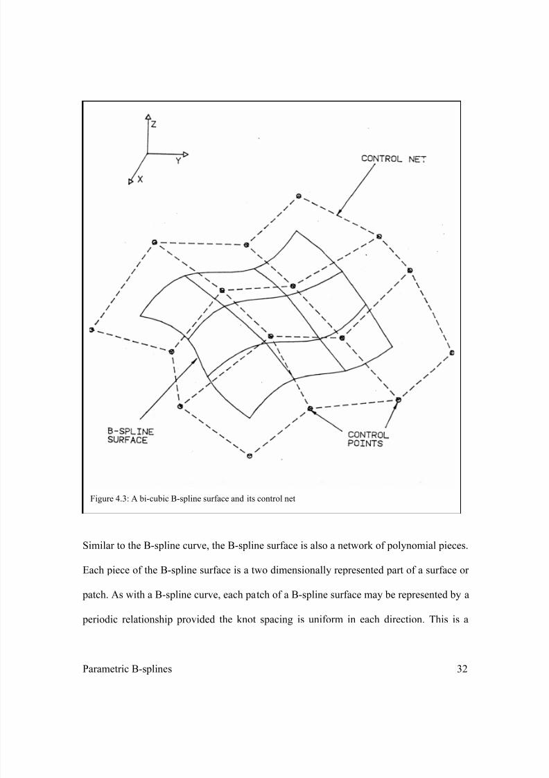
B-spline curve, the B-spline surface approximates the shape of the control net. Figure 4.3
shows a bicubic B-spline surface and the corresponding control net.
7/27/2019 B-spline - Chapter 4.pdf
http://slidepdf.com/reader/full/b-spline-chapter-4pdf 12/24
Parametric B-splines 32
Similar to the B-spline curve, the B-spline surface is also a network of polynomial pieces.
Each piece of the B-spline surface is a two dimensionally represented part of a surface or
patch. As with a B-spline curve, each patch of a B-spline surface may be represented by a
periodic relationship provided the knot spacing is uniform in each direction. This is a
Figure 4.3: A bi-cubic B-spline surface and its control net
7/27/2019 B-spline - Chapter 4.pdf
http://slidepdf.com/reader/full/b-spline-chapter-4pdf 13/24
Parametric B-splines 33
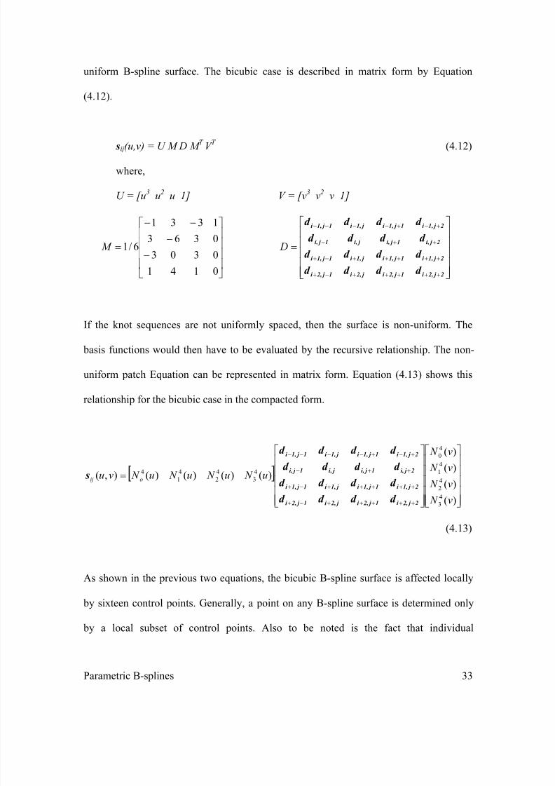
uniform B-spline surface. The bicubic case is described in matrix form by Equation
(4.12).
sij(u,v) = U M D M T
V T
(4.12)
where,
U = [u3
u2
u 1] V = [v3
v2
v 1]
úúúú
û
ù
êêêê
ë
é
-
-
--
=
0141
0303
0363
1331
6/ 1M
ú
úúúú
û
ù
ê
êêêê
ë
é
=
+++++-+
+++++-+
++-
+-+----
2 j 2,i 1 j 2,i j 2,i 1 j 2,i
2 j 1,i 1 j 1,i j 1,i 1 j 1,i
2 j i,1 j i, j i,1 j i,
2 j 1,i 1 j 1,i j 1,i 1 j 1,i
d d d d
d d d d
d d d d
d d d d
D
If the knot sequences are not uniformly spaced, then the surface is non-uniform. The
basis functions would then have to be evaluated by the recursive relationship. The non-
uniform patch Equation can be represented in matrix form. Equation (4.13) shows this
relationship for the bicubic case in the compacted form.
úúúúú
û
ù
êêêêê
ë
é
úúúúú
û
ù
êêêêê
ë
é
=
+++++-+
+++++-+
++-
+-+----
)(
)(
)(
)(
)()()()(),(
4
3
4
2
4
1
4
0
4
3
4
2
4
1
4
v N
v N
v N
v N
u N u N u N u N vuoij
2 j 2,i 1 j 2,i j 2,i 1 j 2,i
2 j 1,i 1 j 1,i j 1,i 1 j 1,i
2 j i,1 j i, j i,1 j i,
2 j 1,i 1 j 1,i j 1,i 1 j 1,i
d d d d
d d d d
d d d d
d d d d
s
(4.13)
As shown in the previous two equations, the bicubic B-spline surface is affected locally
by sixteen control points. Generally, a point on any B-spline surface is determined only
by a local subset of control points. Also to be noted is the fact that individual
7/27/2019 B-spline - Chapter 4.pdf
http://slidepdf.com/reader/full/b-spline-chapter-4pdf 14/24
Parametric B-splines 34
isoparametric curves on a B-spline surface are B-spline curves themselves. For instance,
for a surface defined by Equation (4.10), lines of constant v, i.e., v = v f , are B-spline
curves defined by the Equation (4.14):
)(),(0
u N vuk
i
n
i
f
i f å=
= d s (4.14)
Here f
id are the curve control points. Since this is a parameter curve which lies on the
surface, it can be seen from Equation (4.10) that
åå==
=
m
j
f
k
j ij
n
i
k
i f v N u N v(u,00
)()() d s (4.15)
And therefore
å=
=
m
j
f
k
j ij
f
i v N
0
)(d d (4.16)
This property is used in the thesis to define isoparametric curves lying adjacent to and
normal to the trim boundary for surface interrogation.
Similar to curves, the two knot vectors required to describe a surface have to be
determined using one of the parametrization techniques described earlier. However, due
to the fact that a B-spline surface is a tensor product and constructed of an array of
control points, there are a number of point distances for each individual interval, of each
knot sequence. The solution is typically to calculate a single interval distance based on
the average of all of the point distances.

7/27/2019 B-spline - Chapter 4.pdf
http://slidepdf.com/reader/full/b-spline-chapter-4pdf 15/24
Parametric B-splines 35
4.5 Differential Geometry
The motivation for this topic study is to describe the local curve and surface properties
like curvature. The main tool used for the development of the results is the local
coordinate systems, in terms of which geometric properties are easily described and
studied. As discussed earlier for the case of a B-spline, a curve in E 3
can be described
parametrically as
úúú
û
ù
êêê
ë
é
==)()(
)(
)(u z
u y
u x
u s s , u Î [a,b] Ì R (4.17)
where its Cartesian coordinates x, y, z, are differentiable functions of u (see Figure 4.4). It
is assumed that
0
)(
)(
)(
)( ¹
úúú
û
ù
êêê
ë
é
==
u z
u y
u x
u
s s , u Î [a,b] Ì R (4.18)
where the dots denotes derivatives with respect to u.
Figure 4.4: Parametric curve in space[Fari97].

7/27/2019 B-spline - Chapter 4.pdf
http://slidepdf.com/reader/full/b-spline-chapter-4pdf 16/24
Parametric B-splines 36
An introduction of a special local co-ordinate system called the Frenet frame, linked to a
point s(u) on the curve will significantly facilitate the description of the local curve
properties at the point. The frame (or trihedron) is described by three mutually
perpendicular vectors, t, n and b whose orientation varies as u traces out the curve. The
vector t is called as the tangent vector, n is called main normal vector, and b is called
binormal vector. Figure 4.5 depicts the Frenet frame.
The mathematical relationship of the three vectors with respect to the point s(u) is given
by Equation (4.19)
,
s
s
=t tbn Ù= ,
s s
s s
Ù
Ù
=b , (4.19)
where “Ù” denotes the cross product.
Figure 4.5: The Frenet Frame [Fari97].

7/27/2019 B-spline - Chapter 4.pdf
http://slidepdf.com/reader/full/b-spline-chapter-4pdf 17/24
Parametric B-splines 37
The plane spanned by the point s and the two vectors t, n is called the osculating plane O.
Its equation is given by
úû
ùêë
é
0011
s s sr
det = [ ] s , s s,-r det = 0,
where r denotes any point on O. Its parametric form is
O (u,v) = s s s vu ++ (4.20)
Figure 4.6 explains the relation between the osculating plane and the three mutually
perpendicular vectors and two other planes called the normal plane and the rectifying
plane. The normal and the rectifying planes are perpendicular to each other and each of
them is perpendicular to the osculating plane in turn. The normal and the binormal
vectors determine the normal plane. It is that plane which passes through a point s(u) on
the curve and is perpendicular to the tangent line to the curve at that point. The tangent
and the binormal vectors determine the rectifying plane.
Letting the Frenet frame vary with u provides a good idea of the curve’s behavior in
space. The rate at which the Frenet frame moves with respect to the parameter u gives a
measure of the Curvature and the Torsion of the curve. Curvature (k) is the rate of
turning of the tangent vector and is given by the relation
k = k(u) = 3
s
ss
Ù
(4.21)

7/27/2019 B-spline - Chapter 4.pdf
http://slidepdf.com/reader/full/b-spline-chapter-4pdf 18/24
Parametric B-splines 38
Torsion (t) is a measure of the amount of rotation of the osculating plane. In other words
torsion is a quantity, which indicates whether the curve is twisting rapidly or slowly. It is
expressed mathematically as
t = t(u) =2
det
ss
]s,s,s[
Ù
(4.22)
Figure 4.6: Relation between the normal plane, osculating plane and rectifying plane [Fari97].

7/27/2019 B-spline - Chapter 4.pdf
http://slidepdf.com/reader/full/b-spline-chapter-4pdf 19/24
Parametric B-splines 39
The curvature, torsion and the three Frenet frame vectors t, n, b are related by the
following set of formulas called the Frenet-Serret formulas (Equation 4.23). Figure 4.7
illustrates these formulas
t¢ = +k n,
n¢ = -k t +t b, (4.23)
b¢ = -t n
A point on a curve where k = 0 is called a point of inflection. Since this point is difficult
to locate in most practical cases, another measure called the curvature minima is
employed in finding a point at which the curvature is close to zero and this point can be
considered to be the inflection point, for all practical purposes.
Figure 4.7: The geometric meaning of the Frenet-Serret formulas [Fari97]

7/27/2019 B-spline - Chapter 4.pdf
http://slidepdf.com/reader/full/b-spline-chapter-4pdf 20/24
Parametric B-splines 40
A curve is said to have curvature minima at a point where the following condition holds
true:
k(ui ) - k(ui-1 ) < 0 Ù k(ui+1 ) - k(ui ) ³ 0 (4.24)
Similarly, a curve is said to have curvature maxima at a point where the following holds
true:
k(ui ) - k(ui-1 ) > 0 Ù k(ui+1 ) - k(ui ) £ 0 (4.25)
4.6 Constraint-based B-spline Inversion
B-spline theory was originally developed to define a curve or a surface that approximates
a set of data points. However, a designer is often more interested in using B-splines for
interpolating a set of data points rather than approximating them. The inversion method
addresses this issue by finding the control points for a B-spline curve or a surface given a
set of data points to be interpolated. This process typically consists of setting up and
solving a system of linear equations that are based on interpolation conditions that are
required by the model data. Yamaguchi gives a solution for the inversion of uniform
cubic splines [Yama88] while Gloudamans [Glou89] extends this to a non-uniform case.
Fleming developed an approach to incorporate end constraints to the set of data points to
give the curve or surface a desired level of continuity [Flem92a] [Flem92b].
7/27/2019 B-spline - Chapter 4.pdf
http://slidepdf.com/reader/full/b-spline-chapter-4pdf 21/24
Parametric B-splines 41
For a cubic curve, the inversion process typically consists of setting up and solving for
n+2 control points on n interpolating data points. n equations can be generated based on
these data point constraints. This is accomplished through a knowledge of the behavior of
B-spline basis functions. As previously described, the basis functions are only locally non
zero and any cubic B-spline interval is effected by, at most, four basis functions. At each
knot value ui, however, only three basis functions are non-zero. Therefore, the value of
each data point si can be represented by the following equation.
1iiiiii1-ii
4
1-iii d u N d u N d u N u++++++ ++= )()()()( 2
4
12
4
22 s , i = 1..n (4.26)
This expression, however, is lacking two conditions needed to solve for the n+2 control
points. These conditions, known as the curve end conditions, typically are expressed in
terms of a zero curvature or a tangency condition.
Hence, the control points can be found by solving the following system of equations as
shown in Equation (4.27):
S = N D (4.27)
úúúúúúú
úúúú
û
ù
êêêêêêê
êêêê
ë
é
·
·
··
úúúúúúú
úúúú
û
ù
êêêêêêê
êêêê
ë
é
·
··=
úúúúúúú
úúúú
û
ù
êêêêêêê
êêêê
ë
é
·
··
+
++++-
1
2
1
0
2
4
12
4
2
4
1
4
4
34
4
24
4
1
3
4
23
4
13
n
2
1
conditionend
)()()(
)()()(
)()()(
0conditionend
end
s
s
s
end
n
nnnnnn
4
0
d
d
d
d
u N u N u N
u N u N u N
u N u N u N
7/27/2019 B-spline - Chapter 4.pdf
http://slidepdf.com/reader/full/b-spline-chapter-4pdf 22/24
Parametric B-splines 42
where,
S = Data points
N = basis function values at the knots
D = control points
Surface inversion is slightly more complex than curve inversion and involves solving for
the rectangular array of control points that interpolate to model data points with respect to
two different bases. This process can be described by the following Equation (4.28):
S = N(v) D NT (u) (4.28)
where
S represents the array of data points and end conditions in both directions.
N(v) represents the basis function matrix of the form in Equation (4.27) as a
function of v.
N(u) represents the basis function matrix with respect to u.
D is the array of control points to be solved for.
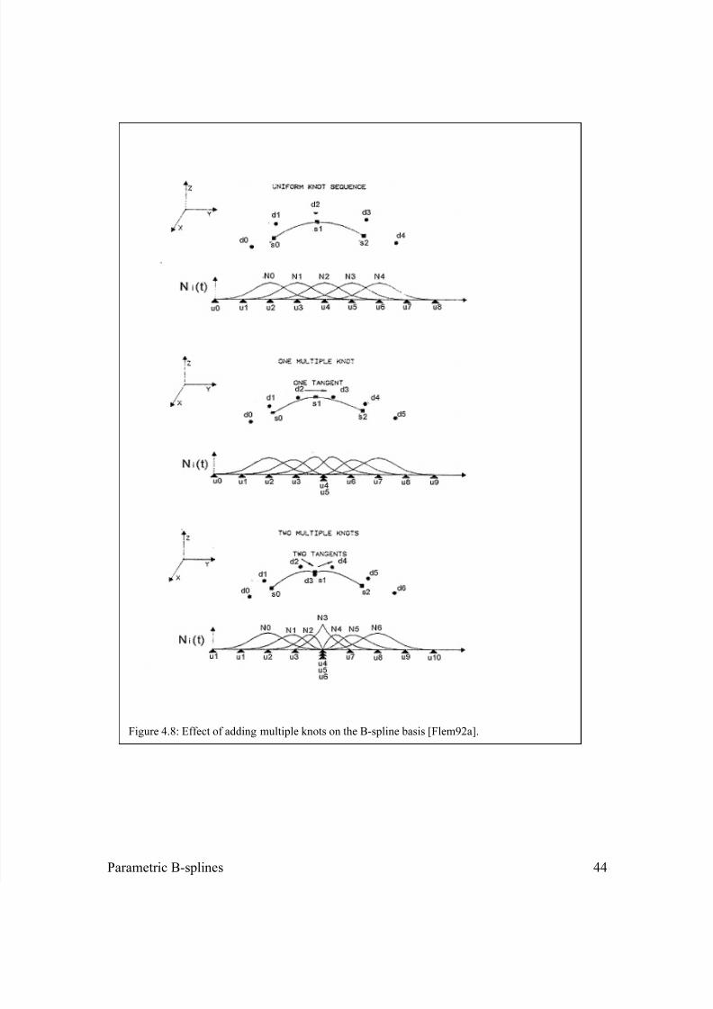
In Fleming’s approach to b-spline inversion, the concept of knot multiplicity is employed.
Knot multiplicity amounts to adding extra knots at points where the continuity has to be
changed. For instance, in order to ensure tangent continuity, one extra knot is required at
the specified point. If instead a sharp corner needs to be modeled, the required knot
multiplicity should be three (two extra knots should be added) to provide with point or C0
continuity at that corner.
7/27/2019 B-spline - Chapter 4.pdf
http://slidepdf.com/reader/full/b-spline-chapter-4pdf 23/24
Parametric B-splines 43
Each time a knot is added, the continuity at that point is reduced. However, the dimension
of the curve is changed and a new basis function is created. Sine a new basis function is
introduced, the number of control points to be solved for also increases which in turn
increases the need for an extra constraint in order to solve for the new control points in
the inversion process. These extra constraints can be provided in terms of tangency
conditions or tangent vectors. For each multiple knot added to the knot sequence, a
tangent vector constraint can be added to the linear system in order to solve for the extra
control points. Thus, for C
1
continuity, one tangent vector is required, whereas for C
0
continuity, two tangent vectors are required; one on either side of the data point
representing the abrupt change in tangency. Figure 4.8 shows the effect adding multiple
knots has on the B-spline basis.
When using continuity constraints, a series of steps have to take place. First, the data
points are parametrized with one of the available techniques (uniform, chord length, etc.).
Next, knot multiplicity is added wherever continuity constraints are required. Once a new
set of knots is defined, all basis functions are calculated so that linear systems including
continuity constraints can be assembled and solved.
7/27/2019 B-spline - Chapter 4.pdf
http://slidepdf.com/reader/full/b-spline-chapter-4pdf 24/24
Figure 4.8: Effect of adding multiple knots on the B-spline basis [Flem92a].


![Bivariate B-spline Outline Multivariate B-spline [Neamtu 04] Computation of high order Voronoi diagram Interpolation with B-spline.](https://static.fdocuments.us/doc/165x107/56649d445503460f94a20e90/bivariate-b-spline-outline-multivariate-b-spline-neamtu-04-computation-of.jpg)

