Elliot Howells Vice President Societies & Campaigns @ SocietiesCSU
Upload
geoffrey-pattersonCategory
view
222download
0
1
B: Overview of Models
Brian Joyce, SEIDenis Hughes, Rhodes University
Mark Howells, KTH
2
Outline
• Brian and Denis describe:– WEAP model of Orange-Senqu– How WEAP model is consistent with other modeling in the region– Initial results showing climate change impacts
• Mark describes:– SAPP model of South African power pool– How SAPP model is consistent with other modeling in the region– Initial results showing climate change impacts

3
Water Modeling
4
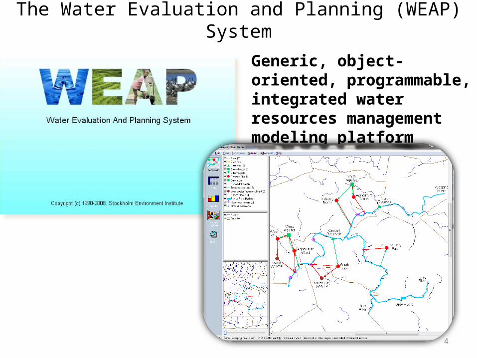
The Water Evaluation and Planning (WEAP) System
Generic, object-oriented, programmable, integrated water resources management modeling platform
5
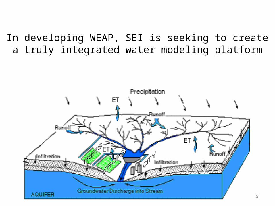
In developing WEAP, SEI is seeking to create a truly integrated water modeling platform

6
WEAP is a globally renowned water modeling platform
WEAP Downloads:
In last day: 14
In last week: 46
In last month: 364
In last 12 months: 3321
Top 10 Forum Members by Country
171 Countries 11602 Members
USA 1090
Iran 982
India 733
Peru 561
China 505
Mexico 473
Colombia 435
Chile 261
Vietnam 258
Germany 243
As of July 2nd 2013
7
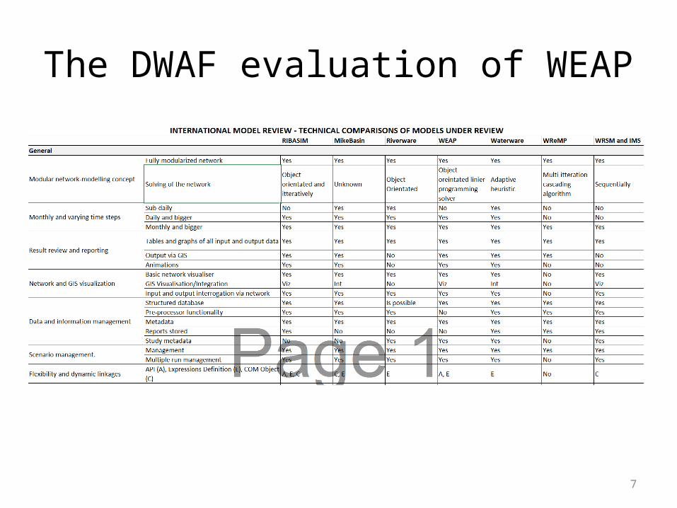
The DWAF evaluation of WEAP

8
Conclusions from DWAF Evaluation
“Even though most of the international models would be able to mimic these water use estimates through their interoperability, the evaluation shows that WEAP and RIBASIM seems to have the most explicitly defined comparative water use definitions to WRSM.”
“WEAP links directly to Qual2K which is currently seen as one of the important eutrophication models and is currently used to assess operational planning in one of the main rivers in South Africa”
“It was found that all the models have similar hydrological and system feature capabilities. MikeBasins, WEAP and Ribasim, however, had strong interoperability capabilities to make provision for any shortcomings in the WRSM capabilities.”
• WEAP water use estimates similar to WRSM
• WEAP water quality routine has regional importance
• Integration of WEAP hydrology seen as benefit
9
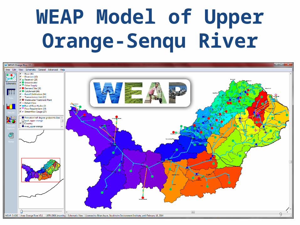
WEAP Model of Upper Orange-Senqu River

10
Two-Step Process for Developing a WEAP Model
from Juizo & Liden, Hydrologic Earth System Sciences (2010)

11
Subcatchment
River Flow
Border
Flow Records
Kraai
Stormberg
Makhaleng
Senqunyane Madibamatso
Matsoku
Seekoei
Leeu
Mopeli
Muelspruit
Brandwater
Lisoloane
Little Caledon
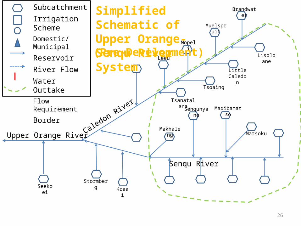
Simplified Schematic of Upper Orange-Senqu River System
Tsanatalana
Tsoaing
(Pre-Development)
Upper Orange River
Senqu River
Caledon River
12
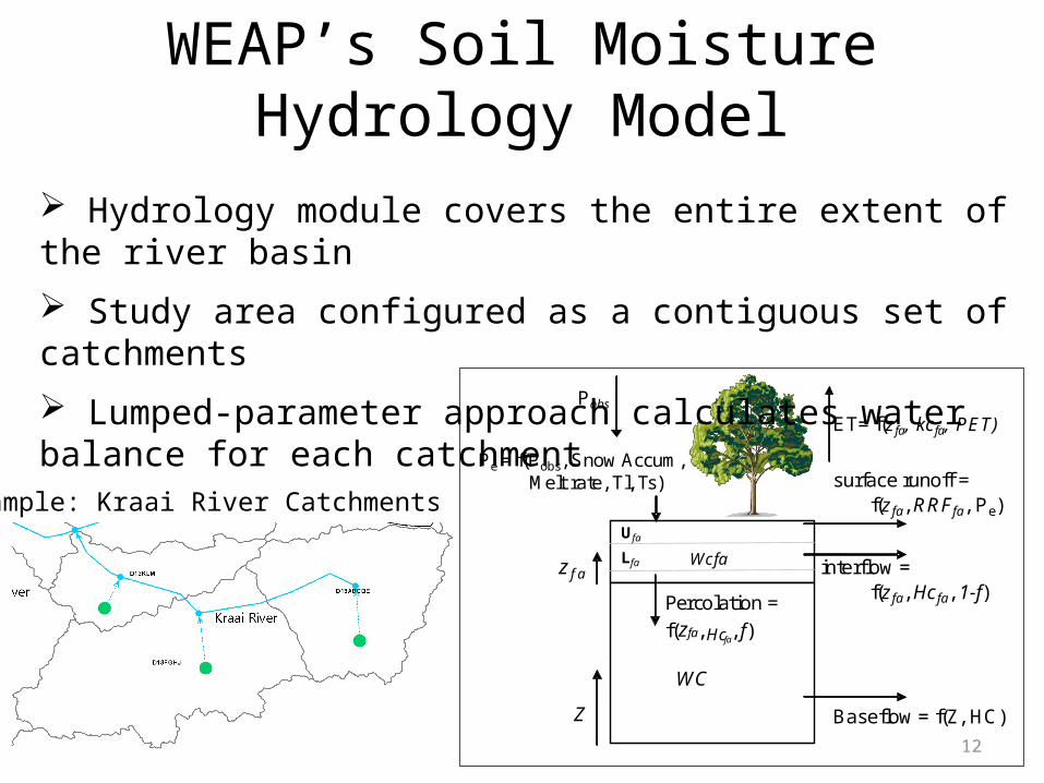
WEAP’s Soil Moisture Hydrology Model
surface runoff =
Baseflow = f(Z, HC)
Ufa
WC
zfa interflow =
Percolation =f( fa Hc
ET= f(zfa, kcfa, PET)
Pe = f(Pobs, Snow Accum,Melt rate, Tl, Ts)
Pobs
Z
f(zfa, RRFfa, Pe)
f(zfa, Hcfa, 1-f)
WcfaLfa
z , )ffa,
Hydrology module covers the entire extent of the river basin
Study area configured as a contiguous set of catchments
Lumped-parameter approach calculates water balance for each catchment
Example: Kraai River Catchments
13
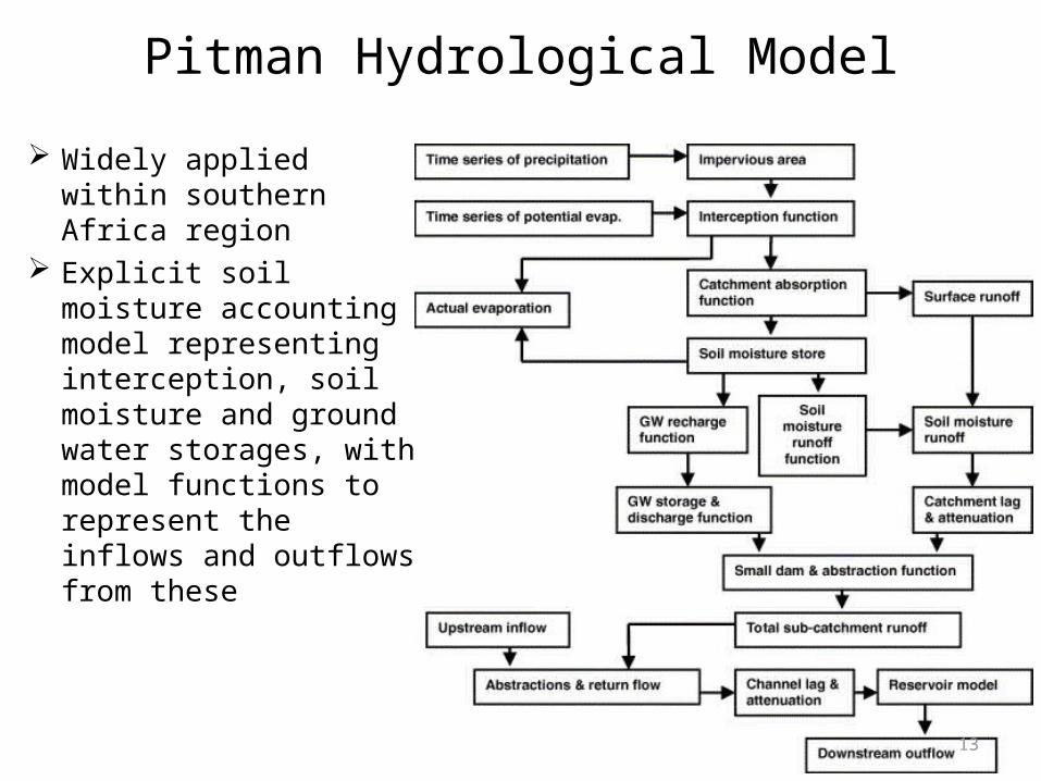
Pitman Hydrological Model Widely applied within
southern Africa region Explicit soil moisture
accounting model representing interception, soil moisture and ground water storages, with model functions to represent the inflows and outflows from these
14
Pitman versus WEAP• Pitman flexibility:
– Represent total stream flow from different sources using built-in components.
• WEAP flexibility:– ‘Expression builder’ allows for additional flexibility
within a relatively simpler model.– Example is using a moisture storage threshold to
limit baseflow outputs and generate zero stream flow in ephemeral rivers.

15
Some specific differences
• Surface runoff generation:– Pitman based on monthly rainfall total only.– WEAP based on combination of monthly rainfall total and
moisture storage state.– Makes comparison between parameter sets of the two
models more difficult.• Flexibility:
– Pitman model flexibility is built-in through more complexity.– WEAP model requires experience in the use of the
‘expression builder’ options.– Ultimately, both require expert knowledge to use effectively.
16
Overall comparison of the two models
• Within the Orange – Senqu system:– Able to calibrate the WEAP model to reproduce very
similar patterns of stream flow as simulated by the Pitman model.
– Most of these achieved with similar water balance components (surface runoff, baseflow, evaporative losses, etc.).
• General conclusions:– Similar uncertainties in the application of the two models.– Given adequate user experience, the calibration efforts
required for the two models are very similar.

17
Orange-Senqu WEAP calibration for natural conditions.
• Learn from Pitman model experience:– Calibration parameters in different parts of the basin.– Pitman model results in un-gauged parts of the basin.– Experience comes from WR90, WR2005, ORASECOM
and some IWR studies in the Caledon River sub-basin.
• Couple Pitman model outputs with observed stream flow data where available (and not impacted by upstream developments) to evaluate WEAP model.

18
Critical headwater inputs: Katse and Mohale dams
Katse Dam inflows Mohale Dam inflows
No substantial differences in the frequency distributions of different monthly flow volumes nor in the seasonal distributions of inflow.

19
Headwaters of the Senqu
Comparisons with ORASECOM simulations for D11 & D16 (WR2005 quaternary catchments)for total period of 1920 to 2005.
Comparisons with observed data at D1H005 (for period 1934 to 1945).
Both WEAP simulations are more than adequate simulations compared to accepted information.

20
Lesotho/South Africa border
Comparisons with ORASECOM
Comparisons with Observed data at D1H009
The ORASECOM comparisons are based on the total simulations period of 1920 to 2005, while the observed data comparisons are based on 1960 to 1992 (avoiding recent development impacts). The results are clearly very favourable.
Time series of monthly flows (WEAP v Observed) suggest that the model is able to capture most of the critical patterns of wet and dry years.
21
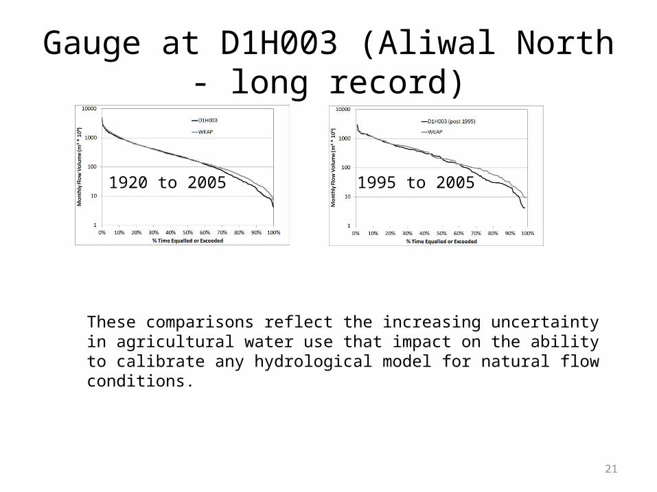
Gauge at D1H003 (Aliwal North - long record)
1920 to 2005 1995 to 2005
These comparisons reflect the increasing uncertainty in agricultural water use that impact on the ability to calibrate any hydrological model for natural flow conditions.
22
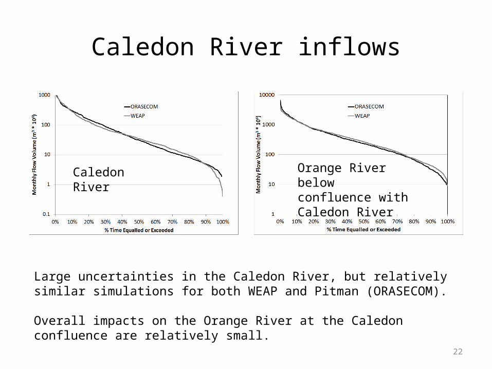
Caledon River inflows
Large uncertainties in the Caledon River, but relatively similar simulations for both WEAP and Pitman (ORASECOM).
Overall impacts on the Orange River at the Caledon confluence are relatively small.
Orange River below confluence with Caledon River
Caledon River
23
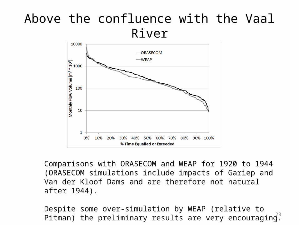
Above the confluence with the Vaal River
Comparisons with ORASECOM and WEAP for 1920 to 1944 (ORASECOM simulations include impacts of Gariep and Van der Kloof Dams and are therefore not natural after 1944).
Despite some over-simulation by WEAP (relative to Pitman) the preliminary results are very encouraging.
24
Natural simulations - refinements• The project team are confident about most of the
simulations.– Particularly in the Senqu River/Lesotho parts of the
basin, when compared with ORASECOM results.• However, there are some areas in the lower parts
of the system where refinements are possible:– Some of these could follow a comparison of simulated
developed conditions with recently observed flows.– Part of the uncertainty is related to the not very well
quantified agricultural use in the South African parts of the Orange and Caledon Rivers.

25
Water infrastructure and demands are nested within the underlying hydrological processes.
Adding Water Resources Management
26
Subcatchment
Irrigation SchemeDomestic/Municipal
Reservoir
River Flow
Water OuttakeFlow Requirement
Border
Kraai
Stormberg
Makhaleng
Senqunyane Madibamatso
Matsoku
Seekoei
Leeu
Mopeli
Muelspruit
Brandwater
Lisoloane
Little Caledon
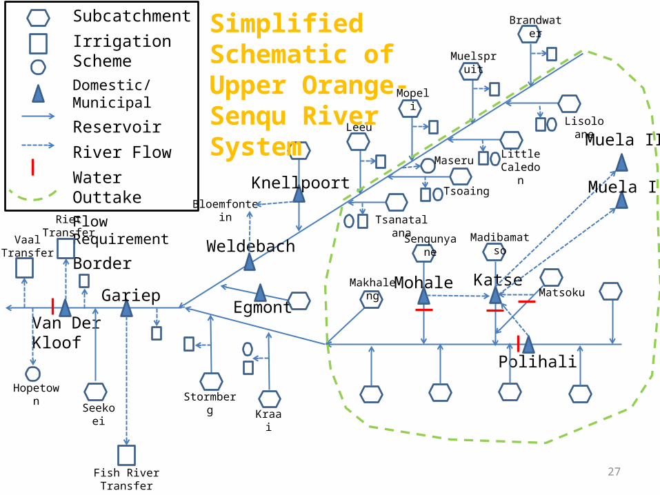
Simplified Schematic of Upper Orange-Senqu River System
Tsanatalana
Tsoaing
(Pre-Development)
Upper Orange River
Senqu River
Caledon River
27
Subcatchment
Irrigation SchemeDomestic/Municipal
Reservoir
River Flow
Water OuttakeFlow Requirement
Border
Gariep
Van Der Kloof
RietTransfer
VaalTransfer
Mohale Katse
Polihali
Muela I
Muela II
Weldebach
Bloemfontein
Knellpoort
Kraai
Stormberg
Makhaleng
Senqunyane Madibamatso
Matsoku
Fish RiverTransfer
Seekoei
Leeu
Mopeli
Muelspruit
Brandwater
Egmont
Lisoloane
Little Caledon
Simplified Schematic of Upper Orange-Senqu River System
Tsanatalana
Hopetown
Tsoaing
Maseru
28
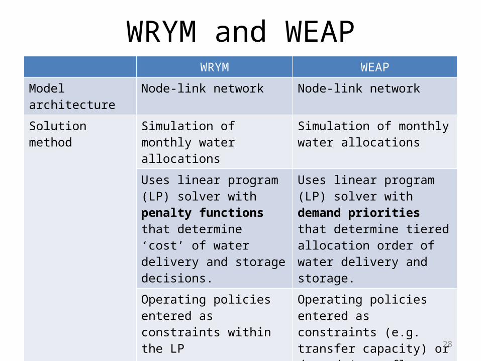
WRYM and WEAPWRYM WEAP
Model architecture Node-link network Node-link network
Solution method Simulation of monthly water allocations
Simulation of monthly water allocations
Uses linear program (LP) solver with penalty functions that determine ‘cost’ of water delivery and storage decisions.
Uses linear program (LP) solver with demand priorities that determine tiered allocation order of water delivery and storage.
Operating policies entered as constraints within the LP
Operating policies entered as constraints (e.g. transfer capacity) or demand (e.g. flow requirement) within the LP
Hydrologic inputs Streamflow timeseries Climate timeseries
Demand projectionsUrban/Domestic
Fixed level of development Transient growth within bounds of uncertainty
Demand projectionsAgriculture
Fixed level of development Climate driven. Subject to transient expansion of area.
29
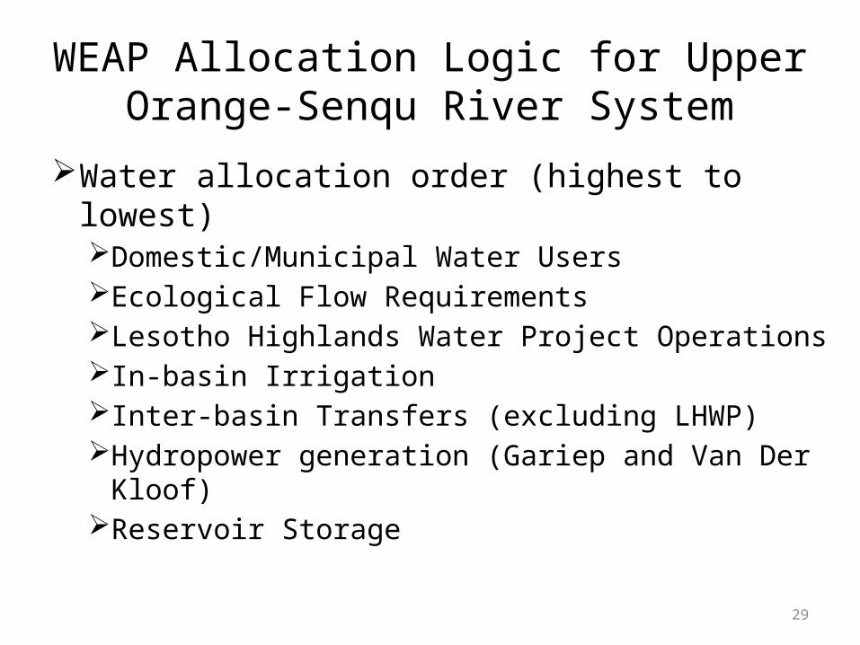
WEAP Allocation Logic for Upper Orange-Senqu River System
Water allocation order (highest to lowest)Domestic/Municipal Water UsersEcological Flow RequirementsLesotho Highlands Water Project OperationsIn-basin IrrigationInter-basin Transfers (excluding LHWP)Hydropower generation (Gariep and Van Der Kloof)Reservoir Storage
30
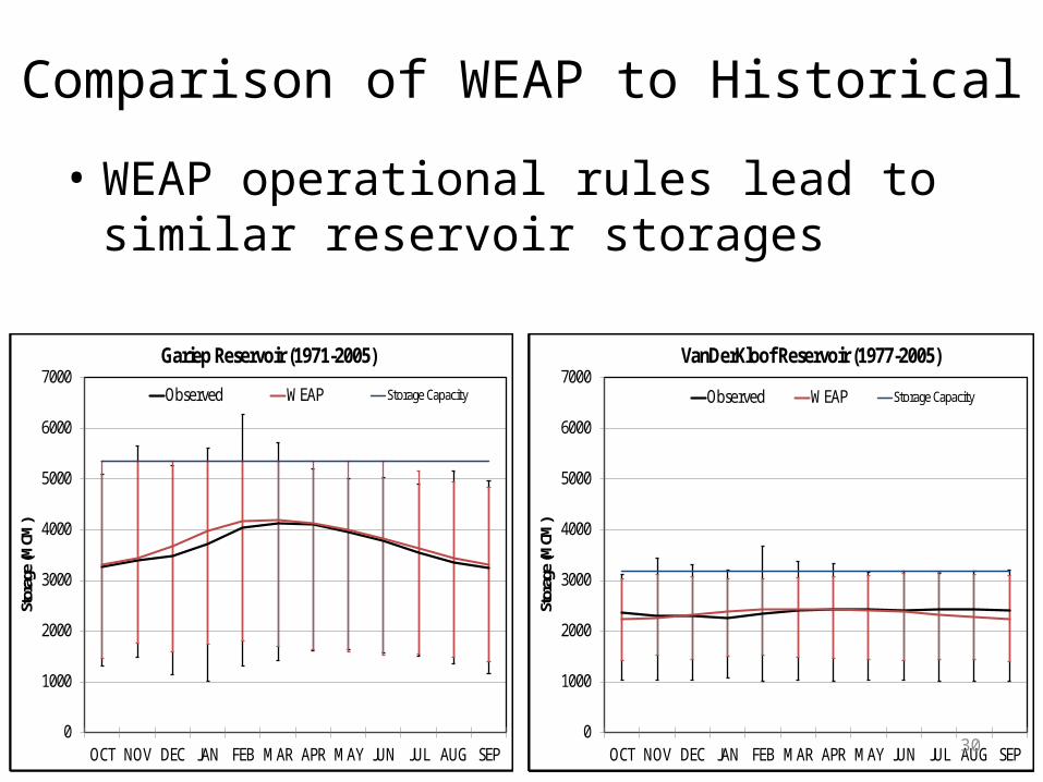
Comparison of WEAP to Historical
• WEAP operational rules lead to similar reservoir storages
0
500
1000
1500
2000
2500
3000
3500
4000
OCT NOV DEC JAN FEB MAR APR MAY JUN JUL AUG SEP
Stor
age (
MCM
)
VanDerKloof Reservoir (1971-2005)
Observed WEAP WRYM Storage Capacity
0
1000
2000
3000
4000
5000
6000
7000
OCT NOV DEC JAN FEB MAR APR MAY JUN JUL AUG SEP
Stor
age (
MCM
)
Gariep Reservoir (1971-2005)
Observed WEAP WRYM Storage Capacity
0
1000
2000
3000
4000
5000
6000
7000
OCT NOV DEC JAN FEB MAR APR MAY JUN JUL AUG SEP
Stor
age
(MCM
)
VanDerKloof Reservoir (1971-2005)
Observed WEAP WRYM Storage Capacity
0
1000
2000
3000
4000
5000
6000
7000
OCT NOV DEC JAN FEB MAR APR MAY JUN JUL AUG SEP
Stor
age
(MCM
)
VanDerKloof Reservoir (1977-2005)
Observed WEAP WRYM Storage Capacity
0
1000
2000
3000
4000
5000
6000
7000
OCT NOV DEC JAN FEB MAR APR MAY JUN JUL AUG SEP
Stor
age
(MCM
)
VanDerKloof Reservoir (1977-2005)
Observed WEAP Storage Capacity
0
1000
2000
3000
4000
5000
6000
7000
OCT NOV DEC JAN FEB MAR APR MAY JUN JUL AUG SEP
Stor
age (
MCM
)
Gariep Reservoir (1971-2005)
Observed WEAP Storage Capacity

31
Energy Modeling

32
An Introduction to OSeMOSYSOpen Source energy MOdeling SYStem • At present there exists a useful, but limited set of
accessible energy systems models. They often require significant investments in terms of human resources, training and software purchases.
• OSeMOSYS is a fully fledged energy systems linear optimisation model, with no associated upfront financial requirements.
• It extends the availability of energy modelling further to researchers, business analysts and government specialists in developing countries.
• An easily ledgible – 500 line long – open source code written in GNU Mathprog with an existing translation into GAMS.
Leading International Partners

33
An Introduction to OSeMOSYS
(6)Constraints
(5) EnergyBalance
(4) Capacity Adequacy
(2)Costs
(3)Storage
(1)Objective
(7)Emissions
Total Capacity
Energy Balance A
Capacity Adequacy A
Discounted Cost
Hydro Facilities
New Capacity
Energy Balance B
Capacity Adequacy B
OperatingCosts
Total Activity
CapitalCosts
Annual Activity
Salvage Value
Reserve Margin
Plain English Description
Mathematical Analogy
Micro Implementation
A Straight forward Building Block based structure• A large user community using and developing different code blocks for OSeMOSYS• Increased tool flexibility with the ability to tailor the code specific modelling
requirements• Easy version change management:
OSeMOSYS to be integrated with a Semantic Media Wiki (SMW) being developed by World Bank-ESMAP
Multiple Levels of Abstraction
Mod
ular
Stru
ctur
e

34
An Introduction to OSeMOSYSUseful for: • Medium- to long-term capacity expansion/investment planning• To inform local, national and multi-regional energy planning• May cover all or individual energy sectors, including heat, electricity and
transport
Main Assumptions• Deterministic linear optimisation model - assumes perfect competition on energy
markets. • Driven by exogenously defined demands for energy services.• These can be met through a range of technologies.• Technologies consume resources, defined by their potentials and costs.• Policy scenarios impose certain technical constraints, economic implications or
environmental targets.• Temporal resolution: consecutive years, split up into ‘time slices’ with specific
demand or supply characteristics, e.g., weekend evenings in summer.
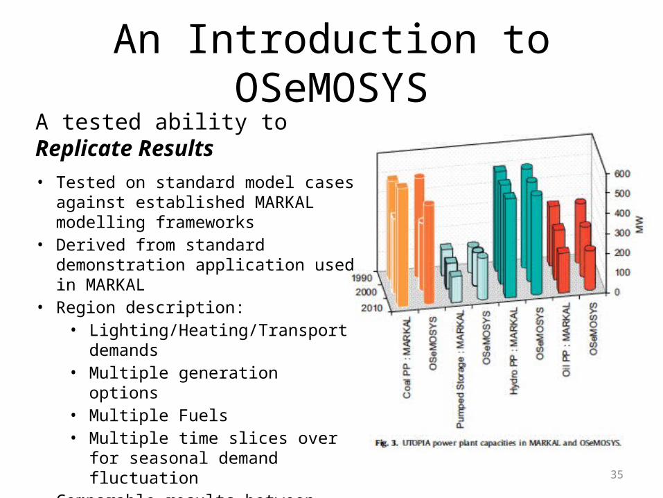
35
An Introduction to OSeMOSYSA tested ability to Replicate Results• Tested on standard model cases against
established MARKAL modelling frameworks• Derived from standard demonstration
application used in MARKAL• Region description:
• Lighting/Heating/Transport demands• Multiple generation options• Multiple Fuels • Multiple time slices over for seasonal
demand fluctuation• Comparable results between both
modelling structures

36
The Southern African Power Pool Model
• Based on latest SAPP consultations
• Hundreds of investment options
• Invests in optimal mix of fossil, hydro, other RE, nuclear and trade to meet growth

37
Energy Model
Water Model
• Energy for water processing • Energy for water pumping• Water available for
hydropower• Water for power plant cooling
C1
• Technology Description Parameters
• Infrastructure description parameters
• Constraints (e.g. resources / emissions etc.)
• Demands per sector
• Detailed optimal cost solution
• Detailed investment plan / capacity plan
• Energy mix and detailed energy flow
• Comprehensive constraints measurement
Inputs Outputs – e.g.
The link to the water modeling
38
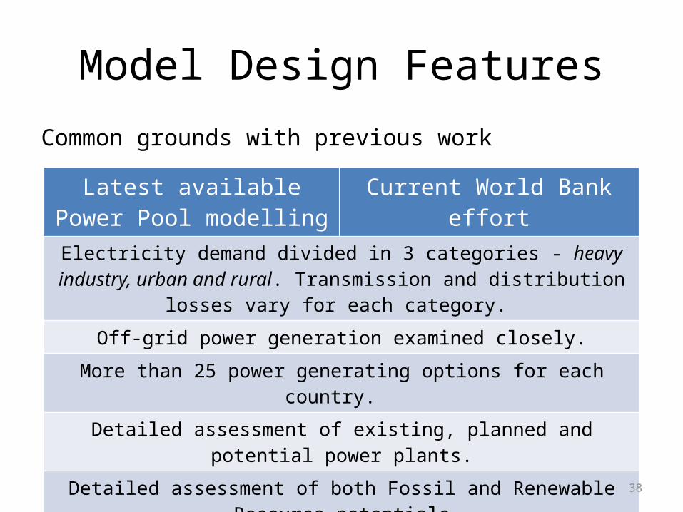
Common grounds with previous work
Model Design Features
Latest available Power Pool modelling
Current World Bank effort
Electricity demand divided in 3 categories - heavy industry, urban and rural. Transmission and distribution losses vary for each category.
Off-grid power generation examined closely.More than 25 power generating options for each country.
Detailed assessment of existing, planned and potential power plants.Detailed assessment of both Fossil and Renewable Resource potentials
39
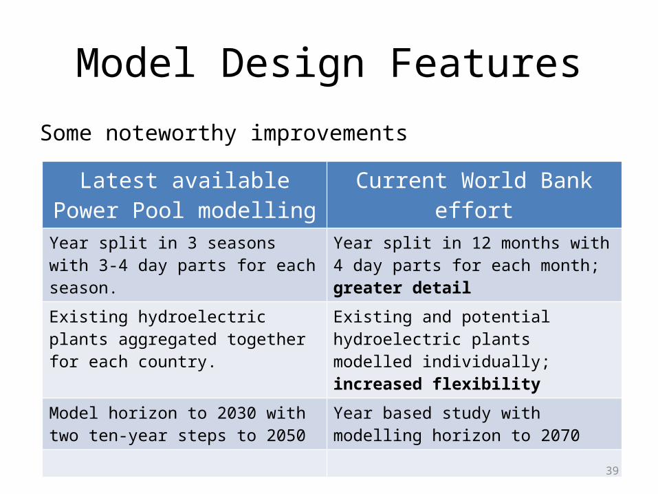
Some noteworthy improvements
Model Design Features
Latest available Power Pool modelling
Current World Bank effort
Year split in 3 seasons with 3-4 day parts for each season.
Year split in 12 months with 4 day parts for each month; greater detail
Existing hydroelectric plants aggregated together for each country.
Existing and potential hydroelectric plants modelled individually; increased flexibility
Model horizon to 2030 with two ten-year steps to 2050
Year based study with modelling horizon to 2070
40
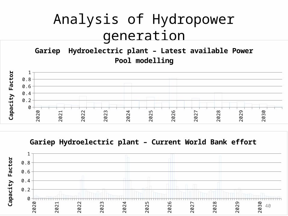
Analysis of Hydropower generation20
20
2021
2022
2023
2024
2025
2026
2027
2028
2029
2030
00.10.20.30.40.50.60.70.80.9
1
Gariep Hydroelectric plant – Latest available Power Pool modelling
Capa
city
Fac
tor
2020
2021
2022
2023
2024
2025
2026
2027
2028
2029
2030
00.10.20.30.40.50.60.70.80.9
1
Gariep Hydroelectric plant – Current World Bank effort
Capa
city
Fac
tor
41
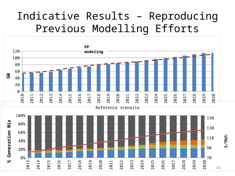
Indicative Results – Reproducing Previous Modelling Efforts
2010
2011
2012
2013
2014
2015
2016
2017
2018
2019
2020
2021
2022
2023
2024
2025
2026
2027
2028
2029
2030
0
20
40
60
80
100
120Latest available SAPP modeling Current World Bank effort
GW
2013
2014
2015
2016
2017
2018
2019
2020
2021
2022
2023
2024
2025
2026
2027
2028
2029
2030
0%10%20%30%40%50%60%70%80%90%
100%
708090100110120130140150
Reference scenario
% G
ener
ation
Mix
$/M
Wh
PP modeling

42
Mozambique Hydro Generation20
11
2012
2013
2014
2015
2016
2017
2018
2019
2020
2021
2022
2023
2024
2025
2026
2027
2028
2029
2030
2031
0
5000
10000
15000
20000
25000
Current World Bank effort
Small HydroHCB North BankMphandaQuedas & OcuaMassingirLuirioOther Historic hydroCahora Basa
GWh
2010
2011
2012
2013
2014
2015
2016
2017
2018
2019
2020
2021
2022
2023
2024
2025
2026
2027
2028
2029
2030
0
5000
10000
15000
20000
25000
Latest available Power Pool modelling
Small HydroHCB North BankMphandaQuedas & OcuaMassingirLuirioOther Historic hydroCahora Basa
GWh

43
Namibia Hydro generation20
10
2011
2012
2013
2014
2015
2016
2017
2018
2019
2020
2021
2022
2023
2024
2025
2026
2027
2028
2029
2030
0
500
1000
1500
2000
2500
3000
Current World Bank effort
Small HydroBaynes
GWh
2010
2011
2012
2013
2014
2015
2016
2017
2018
2019
2020
2021
2022
2023
2024
2025
2026
2027
2028
2029
2030
0
500
1000
1500
2000
2500
3000
Latest available Power Pool modelling
BaynesRuacana
GWh
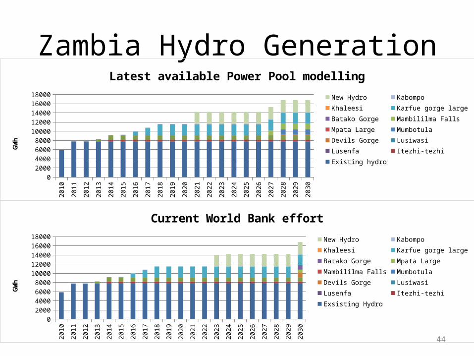
44
Zambia Hydro Generation20
10
2011
2012
2013
2014
2015
2016
2017
2018
2019
2020
2021
2022
2023
2024
2025
2026
2027
2028
2029
2030
0
2000
40006000
800010000
1200014000
1600018000
Latest available Power Pool modellingNew HydroKabompoKhaleesiKarfue gorge largeBatako GorgeMambililma FallsMpata LargeMumbotulaDevils GorgeLusiwasiLusenfaItezhi-tezhiExisting hydro
GWh
2010
2011
2012
2013
2014
2015
2016
2017
2018
2019
2020
2021
2022
2023
2024
2025
2026
2027
2028
2029
2030
0
2000
40006000
800010000
1200014000
1600018000
Current World Bank effortNew HydroKabompoKhaleesiKarfue gorge largeBatako GorgeMpata LargeMambililma FallsMumbotulaDevils GorgeLusiwasiLusenfaItezhi-tezhiExsisting Hydro
GWh
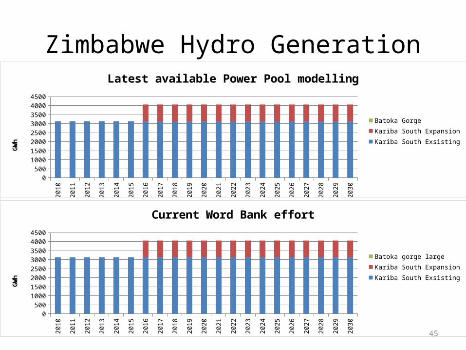
45
Zimbabwe Hydro Generation20
10
2011
2012
2013
2014
2015
2016
2017
2018
2019
2020
2021
2022
2023
2024
2025
2026
2027
2028
2029
2030
0
500
10001500
20002500
30003500
40004500
Latest available Power Pool modelling
Batoka GorgeKariba South ExpansionKariba South Exsisting
GWh
2010
2011
2012
2013
2014
2015
2016
2017
2018
2019
2020
2021
2022
2023
2024
2025
2026
2027
2028
2029
2030
0
500
10001500
20002500
30003500
40004500
Current Word Bank effort
Batoka gorge largeKariba South ExpansionKariba South Exsisting
GWh

46
South Africa Generation Mix 20
10
2011
2012
2013
2014
2015
2016
2017
2018
2019
2020
2021
2022
2023
2024
2025
2026
2027
2028
2029
2030
0%10%20%30%40%50%60%70%80%90%
100%
Latest available Power Pool modelling
NuclearRenewablesHydroFossil fuel
Gene
ratio
n M
ix %
2010
2011
2012
2013
2014
2015
2016
2017
2018
2019
2020
2021
2022
2023
2024
2025
2026
2027
2028
2029
2030
0%
10%
20%
30%
40%
50%
60%
70%
80%
90%
100%
Current World Bank effort
NuclearRenewablesHydroFossil fuel
Gene
ratio
n M
ix %

47
Introducing Climate Projections

48
These Model are Sensitive to Assumptions about Future Climate

49
Climate Impact on Hydropower Generation
• Degree of wetness/dryness of future climate will influence hydropower production
0
250
500
750
1000
1250
1500
1750
2011 - 2030 2031 - 2050
GWH
Firm Hydropower GenerationReference Dry Wet
0
500
1000
1500
2000
2500
3000
3500
4000
0% 10% 20% 30% 40% 50% 60% 70% 80% 90% 100%
GW
H
Percent Non-Exceedence
Annual Hydropower Generation (2011-2050)Reference CC Dry CC Wet
Firm
Yie
ld
0
250
500
750
1000
1250
1500
1750
2011 - 2030 2031 - 2050
GWH
Firm Hydropower GenerationReference Dry Wet
0
500
1000
1500
2000
2500
3000
3500
4000
0% 10% 20% 30% 40% 50% 60% 70% 80% 90% 100%
GW
H
Percent Non-Exceedence
Annual Hydropower Generation (2011-2050)Reference CC Dry CC Wet
Firm
Yie
ld

50
• Irrigation requirements are higher as less water is naturally available within the soil
200
210
220
230
240
250
260
270
280
Dry Dry Wet Wet
Reference 2011-2030 2031-2050 2011-2030 2031-2050
Mill
ion
Cubi
c M
eter
s
Average Irrigation DemandShortage Supply
Climate Impact on Irrigation Requirements

512010
2011
2012
2013
2014
2015
2016
2017
2018
2019
2020
2021
2022
2023
2024
2025
2026
2027
2028
2029
2030
0%
10%
20%
30%
40%
50%
60%
70%
80%
90%
100%
40
80
120
160
200
240
Dry CC
% G
ener
ation
Mix
$/M
Wh
0% 0Fossil fuel Nuclear Renewables Hydro ACOE
2010
2011
2012
2013
2014
2015
2016
2017
2018
2019
2020
2021
2022
2023
2024
2025
2026
2027
2028
2029
2030
0%
10%
20%
30%
40%
50%
60%
70%
80%
90%
100%
40
80
120
160
200
240
Hist CC%
Gen
erati
on M
ix
$/M
Wh
2010
2011
2012
2013
2014
2015
2016
2017
2018
2019
2020
2021
2022
2023
2024
2025
2026
2027
2028
2029
2030
0%
10%
20%
30%
40%
50%
60%
70%
80%
90%
100%
40
80
120
160
200
240
Wet CC
% G
ener
ation
Mix
$/M
Wh

52
- Lesotho - Climate ChangeNuclear Renewables Hydro Fossil fuel
MW
2010
2011
2012
2013
2014
2015
2016
2017
2018
2019
2020
2021
2022
2023
2024
2025
2026
2027
2028
2029
2030
-2500
-2000
-1500
-1000
-500
0
500
1000
1500
2000
2500
Dry Climate Change vs Historical
GWh
2010
2011
2012
2013
2014
2015
2016
2017
2018
2019
2020
2021
2022
2023
2024
2025
2026
2027
2028
2029
2030
-2500
-2000
-1500
-1000
-500
0
500
1000
1500
2000
2500
Wet Climate Change vs HistoricalGW
h
2010
2011
2012
2013
2014
2015
2016
2017
2018
2019
2020
2021
2022
2023
2024
2025
2026
2027
2028
2029
2030
-0.6
-0.4
-0.2
0
0.2
0.4
0.6
Wet Climate Change vs Historical
ACO
E $/
MW
h
2010
2011
2012
2013
2014
2015
2016
2017
2018
2019
2020
2021
2022
2023
2024
2025
2026
2027
2028
2029
2030
-0.4
-0.2
0
0.2
0.4
0.6
0.8
Dry Climate Change vs Historical
ACO
E $/
MW
h

53
We can use our models to explore a range of potential future climate conditions.

54
Previous study of Caledon River using Pitman model indicates a range of possible changes in runoff and critical yield
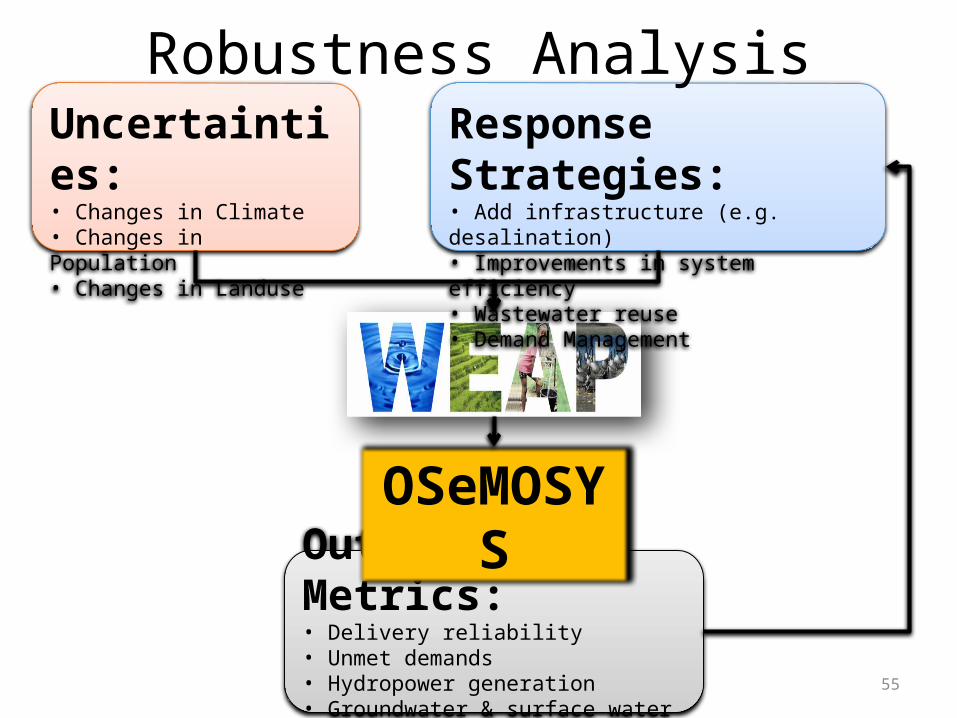
55
Outcome Metrics:• Delivery reliability• Unmet demands• Hydropower generation• Groundwater & surface water storage
Uncertainties: • Changes in Climate• Changes in Population• Changes in Landuse
Response Strategies:• Add infrastructure (e.g. desalination)• Improvements in system efficiency• Wastewater reuse• Demand Management
Robustness Analysis
OSeMOSYS