Journal of Mathematical Sciences, Vol. 176, No. 5, August, 2011

AXIALLY SYMMETRIC TEMPERATURE STRESSES IN AN ELASTIC ISOTROPIC CYLINDER OF FINITE LENGTH

V. V. Meleshko,1 Yu. V. Tokovyy,2 and J. R. Barber3 UDC 539.3

We consider an axially symmetric problem of the thermostressed state of a solid cylinder of finite length with a load-free surface. Using the method of superposition, we have constructed the complete analyti-cal solution of this problem, which is reduced to the solution of a system of linear algebraic equations. We have proposed a method for determining the asymptotic behavior of coefficients in these systems, which enables us to develop an efficient algorithm for the calculation of stresses in the cylinder, includ-ing regions near its end-face circles. Typical examples are considered.

1. Introduction

Beginning from the middle of the 20th century, the problem of thermal stresses in structural elements has been attracting much attention due to important practical problems in the development of new designs of steam and gas turbines, jet and rocket engines, nuclear reactors, etc. Elements of these structures operate under condi-tions of nonuniform and most often nonstationary heating, where there arise temperature gradients and different thermal expansions of their separate parts. Such a nonuniform thermal expansion cannot proceed freely in an elastic body and, therefore, induces heat (thermal, temperature) stresses. Information on the level and character of the action of heat stresses is necessary for the comprehensive analysis of strength of structures.

On the other hand, the study of thermoelasticity as an independent branch of the theory of elasticity began fairly long ago: linear equations for taking into account the influence of heating were deduced independently by Duhamel [25] and Neumann [36]. The nonuniformity of heating of an elastic isotropic body leads to the appear-ance of additional terms, proportional to the temperature, in the Hooke law and a fictitious force, proportional to the temperature gradient, in the Lamé equations for displacements. From that time, the typical problems of thermoelasticity permanently found their place in the classical and present-day textbooks on the theory of elas-ticity, e.g., by Timoshenko [19, Subsec. 66], [43, Subsec. 65, 113–115], [44, Subsec. 148–164], Papkovich [16, Sec. IV, Subsec. 10, 11, Sec. VI, Subsec. 3, Sec. IX, Subsec. 11–13, Sec. X, Subsec. 3, 15, 16], Barber [22, Sec. 14, 22], and Sadd [40, Sec. 12]. In addition, numerous books are devoted to such problems: the textbooks on thermoelasticity by Kovalenko [7, 8, 31] and Hetnarski and Eslami [28] and a series of domestic [1, 10, 12, 13, 17] and foreign [23, 24, 26, 30, 34, 37–39] monographs, containing a detailed bibliography on this subject.

In these works, most attention was given to studying the thermostressed state of an elastic body under con-ditions of a plane problem: plane deformation of a long body of constant cross section, where the thermal proc-esses are independent of the longitudinal coordinate, and the (generalized) plane stressed state of a thin simply connected isotropic plate of constant thickness. Plane quasistatic problems of thermoelasticity in stresses for a known temperature field and in the absence of surface force loads on the body contour are reduced to an inho-

1 Shevchenko National University of Kyiv, Kyiv, Ukraine. 2 Pidstryhach Institute for Applied Problems of Mechanics and Mathematics, Ukrainian National Academy of Sciences, Lviv, Ukraine. 3 University of Michigan, Ann-Arbor, USA.

Translated from Matematychni Metody ta Fizyko-Mekhanichni Polya, Vol. 53, No. 1, pp. 120–137, January–March, 2010. Original arti-cle submitted January 9, 2010.

646 1072-3374/11/1765–0646 © 2011 Springer Science+Business Media, Inc.

AXIALLY SYMMETRIC TEMPERATURE STRESSES IN AN ELASTIC ISOTROPIC CYLINDER OF FINITE LENGTH 647

mogeneous biharmonic equation in a single scalar function for zero values of this function and its normal deriva-tive over the entire boundary [14].

Broad investigations of the three-dimensional problems of thermoelasticity for a finite isotropic cylinder began in the second half of the 20th century in connection with the development of nuclear power engineering [3, 20, 26]. Thermal stresses in the fuel rods of nuclear reactors are fairly high, and, therefore, it is necessary to take them into account for carrying out strength analysis in a three-dimensional temperature field. The influence of end faces of a finite cylinder, free of force loads, for axially symmetric temperature distribution was studied by different analytical and numerical methods [21, 29, 33, 45]. Here, only the radial change in the temperature was studied, and it, generally speaking, does not satisfy the Laplace equation. The general representation of sta-tionary axially symmetric temperature field was considered in [41, 42], where (with extra awkwardness, in our opinion) the solution of the problem was constructed by using the method of superposition. In addition, the ex-ample of a “cube-like” cylinder with a given constant temperature “spot” on its end faces was analyzed. The principal idea of the method of superposition for axially symmetric problems in a finite cylinder lies in using sums of the Fourier and Bessel–Dini series in the complete systems of trigonometric and Bessel functions with respect to the axial and radial coordinates. Each of these series satisfies identically the Lamé equilibrium equa-tions in the region under consideration and has a sequence of coefficients sufficient for satisfying two arbitrary force boundary conditions for the normal and tangential stresses on the end faces and lateral surface of the cyl-inder. Due to the mutual crossing nonorthogonality of functions in these series, the expression for coefficients of one series depends on all coefficients of another and vice versa. This fact leads to the necessity of solving an infinite system of linear algebraic equations, which expresses the dependence between coefficients of the Fourier and Bessel – Dini series, on the one hand, and the applied loads, on the other. Such a system was solved by simple truncation, i.e., using the algorithm of simple reduction. Note that the accuracy of satisfying the bound-ary conditions on the cylinder surface, especially near the end-face circle, was not controlled in any way.

In paper [4], which was later used in textbooks [7, Subsec. 7.3; 8, Subsec. 45; 31, Subsec. 6.2], the method of superposition was used with appropriate analysis of the asymptotics of behavior of the coefficients of these series for large numbers. In particular, it was established that these coefficients tend to a certain common con-stant quantity, which, generally speaking, is not equal to zero. Hence, direct use of the algorithm of simple re-duction for any quantity of equations does not enable one to evaluate correctly the behavior of all coefficients, which is indispensable for clarifying the convergence of these series near boundaries. Koyalovich in his classi-cal treatise [11] considered a typical infinite system, corresponding to the biharmonic problem for a rectangular region, and developed a special theory of limitants, which enables one to determine the upper and lower bounds for all unknown coefficients by the solution of a finite system. In the monograph by Grinchenko [6, Sub-sec. 10], a detailed algorithm of this procedure is presented for determination of the stresses in the entire cylin-der, including its boundary; these results in the form of tables and plots already became canonical. However, in this study, only a quadratic relation temperature vs. radius, independent of the axial coordinate, was chosen, which leads to a thermostressed state of the cylinder that is symmetric with respect to the median plane. In this case, the stationary Laplace equation for the temperature is not satisfied, and, therefore, this canonical example should be considered as a test one in evaluating the possibilities of other analytical and numerical approaches. It is worth noting that the problem of a cylinder, rotating around its central axis with a constant angular velocity [5], is completely identical to the mentioned temperature problem.

The aim of the present work is twofold. First, we consider the complete (symmetric and antisymmetric with respect to the median plane) thermostressed state of a finite cylinder with a surface free of force loads in a sta-tionary temperature field, satisfying the Laplace equation. Second, we improve and somewhat simplify the algo-rithm of calculation of the stresses, based on a more complete use of the law of asymptotic behavior of the coef-ficients, which are determined in the solution of correctly truncated finite system of linear algebraic equations. We also consider specific examples of the application of this algorithm.

648 V. V. MELESHKO, YU. V. TOKOVYY, AND J. R. BARBER

2. Statement of the Thermoelastic Problem and Its Reduction to a Force Problem

Consider an axially symmetric problem of the elastic equilibrium of a solid isotropic cylinder, occupying a domain 0 � r � a , 0 � � � 2� , �h � z � h in the cylindrical coordinate system (r,�, z) . The cylinder is sub-jected to the action of a temperature field T = T (r, z) in the absence of body and surface forces. For this prob-

lem, the radial ur (r, z) and axial uz (r, z) components of the vector of elastic displacements u(r, z) are de-

termined from the Lamé equations [7]

μ�2ur + (� + μ) ���r� μ

ur

r2� (3� + 2μ)�T

�T�r

= 0 ,

μ�2uz + (� + μ) ���z� (3� + 2μ)�T

�T�z

= 0 (1)

under homogeneous boundary conditions for the normal �r and � z and tangential �rz components of the

stress tensor:

�r = 0, �rz = 0, r = a ,

� z = 0, �rz = 0, z = ± h . (2)

Here,

� = 1r��r (rur ) +

�uz

�z

is the volume expansion,

�2 = �2

�r2+ 1

r��r

+ �2

�z2

is the axially symmetric Laplace operator, � and μ are the Lamé elastic constants, and � and �T are

Poisson’s ratio and the coefficient of linear temperature expansion, respectively. The components of the stress tensor are determined via displacements as

�r = 2μ�ur

�r+ �� � (3� + 2μ)�T T , �� = 2μ

ur

r+ �� � (3� + 2μ)�T T ,

� z = 2μ�uz

�z+ �� � (3� + 2μ)�T T , �rz = μ

�ur

�z+�uz

�r�

� �

. (3)

Since the original problem (1), (2) is linear, we may represent the components of the displacement vector as

ur = ur� + ur

(T ) , uz = uz� + uz

(T ) ,

AXIALLY SYMMETRIC TEMPERATURE STRESSES IN AN ELASTIC ISOTROPIC CYLINDER OF FINITE LENGTH 649

where terms with superscript “ (T ) ” indicate the presence of temperature gradients and satisfy inhomogeneous

equations (1). According to (3), these displacements lead to the appearance of temperature stresses [in what fol-lows, also with superscript “ (T ) ”] and, as a result, induce certain external forces on the lateral surface and end

faces of the cylinder. The components of the displacement vector marked with superscript “�” satisfy homo-geneous equations (1), compensating the influence of stresses on the cylinder surface mentioned above in such a way that conditions (2) be satisfied. Thus, we come to boundary conditions

�r� = f (z), �rz

� = s(z), r = a ,

� z� = g± (r ), �rz

� = p± (r), z = ± h , (4)

where f (z) = �� r(T ) (a, z) , s(z) = � �rz

(T ) (a, z) , g± (r) = �� z(T ) (r,±h) , p± (r) = � �rz

(T ) (r,±h) , and the

stresses marked with “�” are determined from (3) in the absence of temperature terms. Note that the conditions of elastic equilibrium impose certain constraints on the right-hand sides of condi-

tions (4), which can be written as

a s(z)dz�h

h

� = r(g� (r) � g+ (r))dr0

a

� ,

a f (z)dz�h

h

� + r(p+ (r) � p� (r))dr0

a

� = ��� dz dr

�h

h

�0

a

� . (5)

There exists a general procedure [2] of integration of the equilibrium equations for deriving integral conditions for the components of the stress tensor.

The “temperature” solution of Eqs. (1) can be found using the Papkovich [15]–Goodier [27] potential � = �(r, z) in the form

ur(T ) = ���r , uz

(T ) = ���z ,

where the function � is a particular solution of the Poisson equation

�2� = 1+ �1� � �T T . (6)

The stresses corresponding to displacements (4) are written in the form

�r(T ) = 2μ �2�

�r2��2��

���

, ��(T ) = 2μ 1

r���r

��2�( ) ,

� z(T ) = 2μ �2�

�z2��2��

���

, �rz(T ) = 2μ �2�

�r�z. (7)

650 V. V. MELESHKO, YU. V. TOKOVYY, AND J. R. BARBER

3. Construction of a Solution of Force Problem

One can construct the components of the displacement vector u� and the corresponding stresses in differ-ent ways. In textbooks on the theory of elasticity and thermoelasticity as well as in special monographs, in par-ticular, [9, 18], devoted exclusively to problems for cylindrical bodies, one can find various approaches to con-structing the general solution of the Lamé equations, which have certain advantages or shortcomings for differ-ent kinds of boundary conditions. In particular, the Love, Weber, Timpe, Papkovich–Neuber, and other stress functions are used here. The Papkovich representation [16] in terms of harmonic scalar and vector functions is used in the textbooks by Kovalenko [7, Subsec. 7.2; 8, Subsec. 45; 31, Subsec. 6.2], and direct integration of the Lamé homogeneous equations (1) in displacements is applied in the monograph by Grinchenko [6, Subsec. 9]. In the case of the problem for a finite cylinder, as, in general, for bodies of finite sizes, the choice of the form of representing the general solution of the Lamé equations is a question of principle only in the sense that the solu-tion being obtained has to contain a sufficient quantity of functions with arbitrary coefficients to enable one to satisfy the boundary conditions (4) over the entire cylinder surface.

In the present work, we use the Love function � = �(r, z) , which satisfies the homogeneous biharmonic

equation [32, Subsec. 99]

�2�2� = 0 .

Then the radial and axial displacements are given by

ur� = � 1

2μ�2��r�z

, uz� = 1

2μ 2(1� �)�2� � �2��z2

���

�

,

and the components of the stress tensor are calculated as

�r� = �

�z��2� � �2�

�r2

���

�

, � z� = �

�z(2 � �)�2� � �2�

�z2

���

�

,

��� = �

�z��2� � 1

r���r

�

� , rz

� = ��r

(1� �)�2� � �2��z2

��

��

. (8)

In the solution of the boundary-value problem, it is reasonable to decompose the stressed state of the cylin-der into parts that are respectively symmetric and antisymmetric, with respect to the plane z = 0 , representing its temperature field as

T (r, z) = T {e} (r, z) + T {o} (r, z) , (9)

where T{e}(r, z) = (T (r, z)+ T (r,�z))/ 2 is the part of temperature distribution symmetric with respect to the

plane cross section of the cylinder z = 0 , and T{o}(r, z) = (T (r, z)� T (r,�z))/ 2 is its antisymmetric part.

3.1. Temperature Distribution Symmetric with Respect to the Coordinate z . Consider the case of elastic

equilibrium of a cylinder subjected to the action of the temperature field T{e}(r, z) . This case was considered

AXIALLY SYMMETRIC TEMPERATURE STRESSES IN AN ELASTIC ISOTROPIC CYLINDER OF FINITE LENGTH 651

in detail in [6, Subsec. 10; 7, Subsec. 7.2; 31, Subsec. 6.2], and, therefore, we here describe it schematically, fo-cusing our attention on separate elements that were passed over.

A stationary (or instantaneous) symmetric temperature field can always be represented by the Fourier series

T {e} (r, z) = Tn

{e} (r)cos knzn=0

�

� , (10)

where

T0

{e} (r) = 12h

T {e} (r, z)dz�h

h

� , Tn{e} (r) = 1

hT {e} (r, z)cos knz dz

�h

h

� ,

kn = n�/h, n = 1, 2,….

Using the given temperature field, we determine a particular solution of Eq. (6) for the thermoelastic potential written in a similar way:

�(r, z) = 1+ �1� � �T �n (r)cos knz

n=0

�

� . (11)

Substitution of (10) and (11) in Eq. (6) with regard for the completeness of the system {cos knz, n = 0,1,…}

for this case gives a differential equation

���n (r) + 1

r��n (r) � kn

2�n (r) = Tn{e} (r), n = 0, 1, 2,… ,

which has solutions presented in [7, Subsec. 7.3]. Here and below, we denote by a prime the differentiation of a function of one variable. The expressions for stresses (7) have the form

�r

(T ) = K [ ���n (r) � Tn{e} (r)]cos knz

n=0

�

� , ��(T ) = K 1

r��n (r) � Tn

{e} (r)�

� �cos knz

n=0

�

� ,

� z

(T ) = �K [kn2�n (r) + Tn

{e} (r)]cos knzn=0

�

� , �rz(T ) = �K kn ��n (r)sin knz

n=0

�

� , (12)

where K = 2μ(1+ �)�T /(1� �) .

With regard for expressions (12), we represent the right-hand sides of “force” load (4) in the form of expan-sions

f (z) = (�1)n fn cos knz,n=0

�

� s(z) = (�1)n sn sin knzn=1

�

� ,

g+ (r) = g� (r) = g(r), g(r) = g0 + g j

J0 (� j r)

J0 (� ja),

j=1

�

� p± (r) � 0 (13)

652 V. V. MELESHKO, YU. V. TOKOVYY, AND J. R. BARBER

with obvious expressions for the coefficients fn and sn [the multiplier (�1)n is introduced to simplify the

writing of subsequent relations]. Then we obtain expressions for g0 and g j by the standard expansion of

functions kn2�n (r)+ Tn

{e}(r) into Bessel–Dini series in the complete system of functions {1 , J0 (� j r) ,

j = 1,2,…} and subsequent summation over the subscript n . Here, � j are the positive roots of equation

J1(�a) = 0 , numbered in ascending order, and J0 and J1 are the zero- and first-order Bessel functions of

the first kind. To construct a solution of the original problem (1), (2) for the temperature field (10), it remains to deter-

mine the components of the stress tensor (8), which satisfy the boundary conditions (4) with right-hand sides (13). We use here the Love function in the form [35]

� = B0z3 + D0r2z + �s + h Yj Rj (z)j=1

�

�J0 (� j r)

� j3J0 (� ja)

+ a (�1)n XnSn (r)n=1

�

� sin knz

kn3

, (14)

where

�s = (�1)n snI0 (knr)I1(kna)

n=1

�

� sin knz

kn3

,

Rj (z) = h coth� jh +2�� j

���

�

sinh� j z

sinh� jh� z

cosh� j z

sinh� jh,

Sn (r) = 2 � �1kn

� aI0 (kna)I1(kna)

���

��

I0 (knr)I1(kna)

+ rI1(knr)I1(kna)

,

B0 , D0 , Yj , Xn , { j,n} = 1,2,… , are unknown coefficients that should be determined from conditions (4)

and (13), and I0 and I1 are the zero- and first-order modified Bessel functions of the first kind. According to

(8) and (14), the corresponding stresses have the form

�r� = 6�B0 + 2(2� �1)D0 +

��z

�2�s ��2�s

�r2

�

� �

��� h Yj �Rj (z)

J1(� j r)

� j2rJ0 (� ja)j=1

�

+

h Yj [� ���Rj (z) + (1� �)� j

2 �Rj (z)]j=1

�

�J0 (� j r)

� j3J0 (� ja)

+ a (�1)n Xn (� �1) ��Sn (r) + �r

�Sn (r) � kn2�Sn (r)�

���

cos knz

kn2

n=1

�

� ,

AXIALLY SYMMETRIC TEMPERATURE STRESSES IN AN ELASTIC ISOTROPIC CYLINDER OF FINITE LENGTH 653

��� = 6�B0 + 2(2� �1)D0 +

z

��2�s �1r�s

r ��

��� + h Yj Rj (z)

J1(� j r)

� j2rJ0 (� ja)j=1

�

�

+

h� Yj [ ���Rj (z) � � j

2 �Rj (z)]j=1

�

�J0 (� j r)

� j3J0 (� ja)

+ a (�1)n Xn � ��Sn (r) + � �1r

�Sn (r) � kn2�Sn (r)�

���

cos knz

kn2

n=1

�

� ,

� z� = 6(1� �)B0 + 4(2 � �)D0 +

��z

(2 � �)�2�s ��2�s

�z2

�

���

�

+

h Yj [(1� �) ���Rj (z)

j=1

�

� + � j2 �Rj (z)]

J0 (� j r)

� j3J0 (� ja)

+ a (�1)n Xn (2 � �) ��Sn (r) + 1r

�Sn (r)( ) � (1� �)kn2Sn (r)�

���

n=1

�

� cos knz

kn2

,

rz� =

r(1� �)�2�s �

2�s

z2

���

��+ h Yj [� Rj (z) + � j

2 Rj (z)]j=1

�

�J1(� j r)

� j2 J0 (� ja)

+

a (�1)n Xn

n=1

�

� 1� �r

(r �Sn (r) ��) � 1r(r �Sn (r))�( ) + �kn

2Sn (r)��

��

sin knz

kn3

. (15)

It is easy to verify that the tangential stresses �rz� satisfy identically the boundary conditions (4) and (13)

on the end faces and lateral surface of the cylinder. Further, satisfying the boundary conditions (4) for the nor-

mal stresses �r� and � z

� , we obtain with the use of (�3), (�12), (�14), (�18), and (�20) two equations

6�B0 + 2(2� �1)D0 = f0 , 6(1� �)B0 + 4(2 � �)D0 = g0 + s0 (16)

and an infinite system of linear algebraic equations

XnPn � Yj4kn

2

(kn2 + � j

2 )2j=1

�

� = fn + snqn , n = 1,2,… ,

Yj� j � Xn

4� j2

(kn2 + � j

2 )2n=1

�

� = � g j � c j , j = 1,2,… , (17)

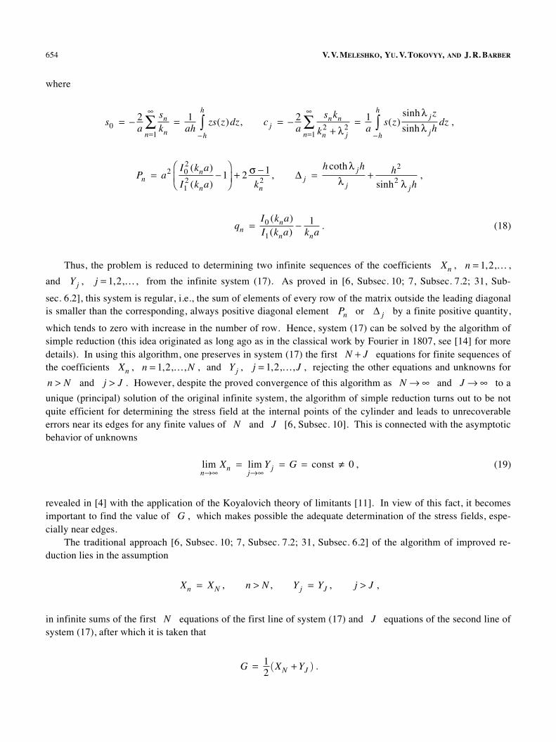
654 V. V. MELESHKO, YU. V. TOKOVYY, AND J. R. BARBER

where

s0 = � 2a

sn

knn=1

�

� = 1ah

zs(z)dz�h

h

� , c j = � 2a

snkn

kn2 + � j

2n=1

�

� = 1a

s(z)sinh� j z

sinh� jhdz

�h

h

� ,

Pn = a2 I02 (kna)

I12 (kna)

�1�

��

�+ 2 � �1

kn2

, � j =h coth� jh

� j+ h2

sinh2 � jh,

qn =I0 (kna)I1(kna)

� 1kna

. (18)

Thus, the problem is reduced to determining two infinite sequences of the coefficients Xn , n = 1,2,… ,

and Yj , j = 1,2,… , from the infinite system (17). As proved in [6, Subsec. 10; 7, Subsec. 7.2; 31, Sub-

sec. 6.2], this system is regular, i.e., the sum of elements of every row of the matrix outside the leading diagonal is smaller than the corresponding, always positive diagonal element Pn or � j by a finite positive quantity,

which tends to zero with increase in the number of row. Hence, system (17) can be solved by the algorithm of simple reduction (this idea originated as long ago as in the classical work by Fourier in 1807, see [14] for more details). In using this algorithm, one preserves in system (17) the first N + J equations for finite sequences of the coefficients Xn , n = 1,2,…, N , and Yj , j = 1,2,…, J , rejecting the other equations and unknowns for

n > N and j > J . However, despite the proved convergence of this algorithm as N � � and J � � to a

unique (principal) solution of the original infinite system, the algorithm of simple reduction turns out to be not quite efficient for determining the stress field at the internal points of the cylinder and leads to unrecoverable errors near its edges for any finite values of N and J [6, Subsec. 10]. This is connected with the asymptotic behavior of unknowns

limn��

Xn = limj��

Yj = G = const � 0 , (19)

revealed in [4] with the application of the Koyalovich theory of limitants [11]. In view of this fact, it becomes important to find the value of G , which makes possible the adequate determination of the stress fields, espe-cially near edges.

The traditional approach [6, Subsec. 10; 7, Subsec. 7.2; 31, Subsec. 6.2] of the algorithm of improved re-duction lies in the assumption

Xn = XN , n > N , Yj = YJ , j > J ,

in infinite sums of the first N equations of the first line of system (17) and J equations of the second line of system (17), after which it is taken that

G = 1

2(XN +YJ ) .

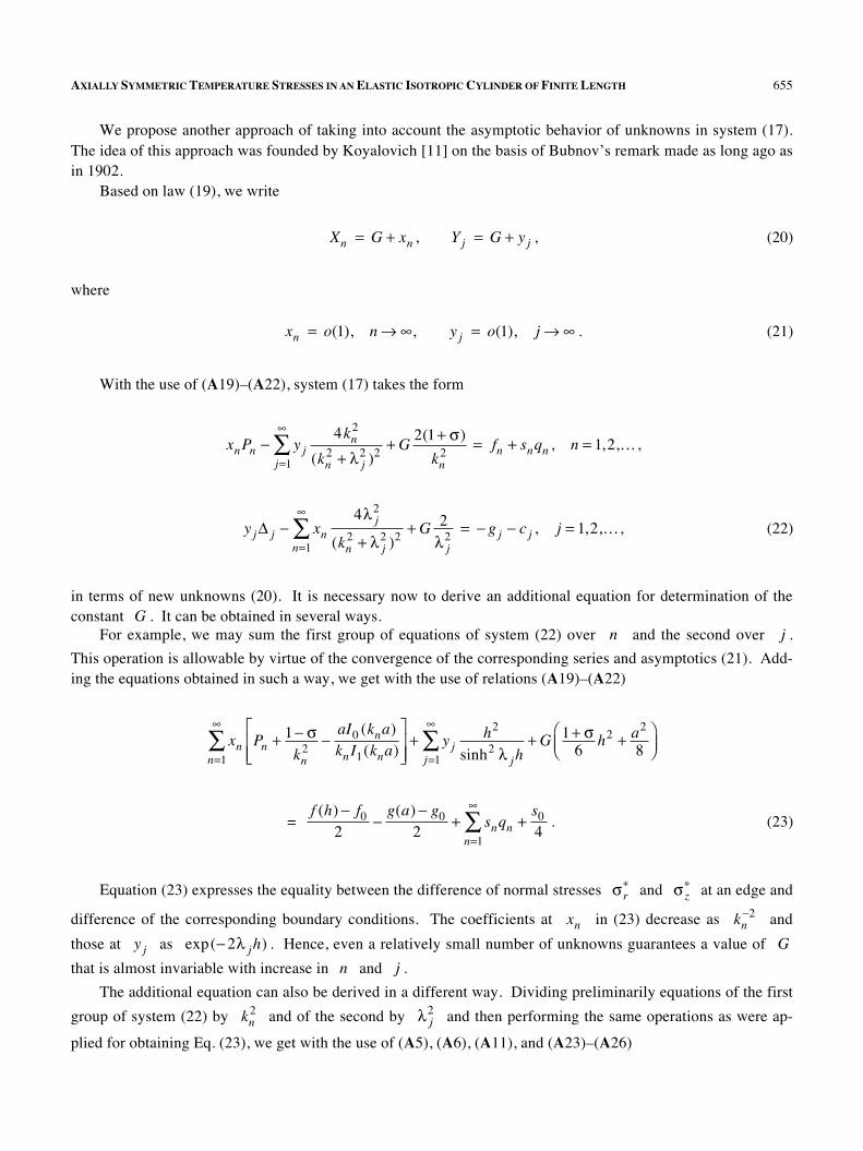
AXIALLY SYMMETRIC TEMPERATURE STRESSES IN AN ELASTIC ISOTROPIC CYLINDER OF FINITE LENGTH 655

We propose another approach of taking into account the asymptotic behavior of unknowns in system (17). The idea of this approach was founded by Koyalovich [11] on the basis of Bubnov’s remark made as long ago as in 1902.

Based on law (19), we write

Xn = G + xn , Yj = G + y j , (20)

where

xn = o(1), n� �, y j = o(1), j � � . (21)

With the use of (�19)–(�22), system (17) takes the form

xnPn � y j4kn

2

(kn2 + � j

2 )2j=1

�

� + G2(1+ �)

kn2

= fn + snqn , n = 1,2,… ,

y j� j � xn

4� j2

(kn2 + � j

2 )2n=1

�

� + G 2� j

2= � g j � c j , j = 1,2,…, (22)

in terms of new unknowns (20). It is necessary now to derive an additional equation for determination of the constant G . It can be obtained in several ways.

For example, we may sum the first group of equations of system (22) over n and the second over j .

This operation is allowable by virtue of the convergence of the corresponding series and asymptotics (21). Add-ing the equations obtained in such a way, we get with the use of relations (�19)–(�22)

xn Pn +1� �

kn2

�aI0 (kna)kn I1(kna)

�

�

���n=1

�

� + y jh2

sinh2 � jhj=1

�

� + G 1+ �6

h2 + a2

8 ��

���

= f (h) � f0

2�

g(a) � g02

+ snqnn=1

�

� +s04

. (23)

Equation (23) expresses the equality between the difference of normal stresses �r� and � z

� at an edge and

difference of the corresponding boundary conditions. The coefficients at xn in (23) decrease as kn�2 and

those at y j as exp(�2� jh) . Hence, even a relatively small number of unknowns guarantees a value of G

that is almost invariable with increase in n and j .

The additional equation can also be derived in a different way. Dividing preliminarily equations of the first

group of system (22) by kn2 and of the second by � j

2 and then performing the same operations as were ap-

plied for obtaining Eq. (23), we get with the use of (�5), (�6), (�11), and (�23)–(�26)

656 V. V. MELESHKO, YU. V. TOKOVYY, AND J. R. BARBER

(1+ �)xn

kn4

n=1

�

� +y j

� j4

j=1

�

� + G 1+ �90

h4 + a4

192���

�

= �h

h

� f (z) 3z2 � h2

24hdz �

0

a

� rg(r) 2r2 � a2

8a2dr +

�h

h

� zs(z)2(z2 � h2 ) � 3

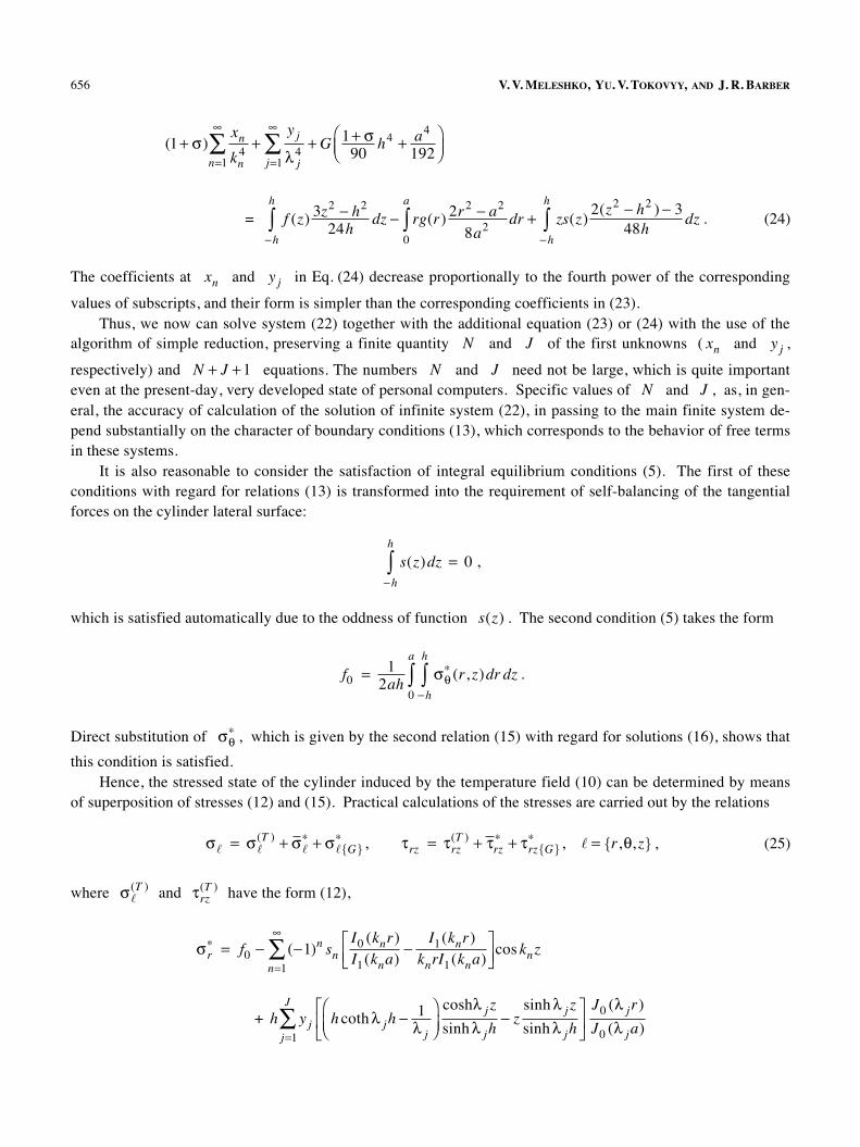
48hdz . (24)

The coefficients at xn and y j in Eq. (24) decrease proportionally to the fourth power of the corresponding

values of subscripts, and their form is simpler than the corresponding coefficients in (23). Thus, we now can solve system (22) together with the additional equation (23) or (24) with the use of the

algorithm of simple reduction, preserving a finite quantity N and J of the first unknowns ( xn and y j ,

respectively) and N + J +1 equations. The numbers N and J need not be large, which is quite important even at the present-day, very developed state of personal computers. Specific values of N and J , as, in gen-eral, the accuracy of calculation of the solution of infinite system (22), in passing to the main finite system de-pend substantially on the character of boundary conditions (13), which corresponds to the behavior of free terms in these systems.

It is also reasonable to consider the satisfaction of integral equilibrium conditions (5). The first of these conditions with regard for relations (13) is transformed into the requirement of self-balancing of the tangential forces on the cylinder lateral surface:

s(z)dz�h

h

� = 0 ,

which is satisfied automatically due to the oddness of function s(z) . The second condition (5) takes the form

f0 = 12ah

��� (r, z)dr dz

�h

h

�0

a

� .

Direct substitution of ��� , which is given by the second relation (15) with regard for solutions (16), shows that

this condition is satisfied. Hence, the stressed state of the cylinder induced by the temperature field (10) can be determined by means

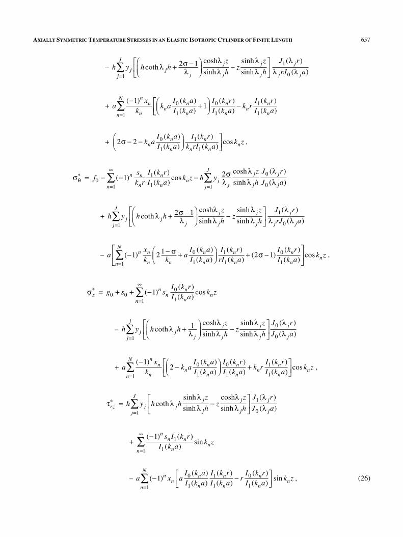
of superposition of stresses (12) and (15). Practical calculations of the stresses are carried out by the relations

�� = ��

(T ) + ��� + ��{G}

� , �rz = �rz(T ) + �rz

� + �rz{G}� , � = {r,�, z} , (25)

where ��(T ) and �rz

(T ) have the form (12),

�r� = f0 � (�1)n sn

I0 (knr)I1(kna)

�I1(knr)

knrI1(kna)��

��cos knz

n=1

�

�

+ h y j h coth� jh �1� j

���

� �

cosh� j z

sinh� jh� z

sinh� j z

sinh� jh

�

�

��

j=1

J

�J0 (� j r)

J0 (� ja)

AXIALLY SYMMETRIC TEMPERATURE STRESSES IN AN ELASTIC ISOTROPIC CYLINDER OF FINITE LENGTH 657

– h y j h coth� jh +2� �1� j

���

� �

cosh� j z

sinh� jh� z

sinh� j z

sinh� jh

�

�

��

j=1

J

�J1(� j r)

� j rJ0 (� ja)

+ a(�1)n xn

knkna

I0 (kna)I1(kna)

+1���

���

I0 (knr)I1(kna)

� knrI1(knr)I1(kna)

��n=1

N

�

+ 2� � 2 � knaI0 (kna)I1(kna)

���

��

I1(knr)knrI1(kna)

��

cos knz ,

��� = f0 � (�1)n sn

knrI1(knr)I1(kna)

cos knzn=1

�

� � h y j2�� j

cosh� j z

sinh� jh

J0 (� j r)

J0 (� ja)j=1

J

�

+ h y j h coth� jh +2� �1� j

���

� �

cosh� j z

sinh� jh� z

sinh� j z

sinh� jh

�

�

��

j=1

J

�J1(� j r)

� j rJ0 (� ja)

– a (�1)n xn

kn2 1� �

kn+ a

I0 (kna)I1(kna)

���

� �

I1(knr)rI1(kna)

n=1

N

� + (2� �1)I0 (knr)I1(kna)

�

�

��cos knz ,

� z� = g0 + s0 + (�1)n sn

I0 (knr)I1(kna)

cos knzn=1

�

�

– h y jj=1

j

� h coth� jh +1� j

���

� �

cosh� j z

sinh� jh� z

sinh� j z

sinh� jh

�

�

��

J0 (� j r)

J0 (� ja)

+ a(�1)n xn

knn=1

N

� 2 � knaI0 (kna)I1(kna)

���

���

I0 (knr)I1(kna)

+ knrI1(knr)I1(kna)

��

��

cos knz ,

�rz� = h y j h coth� jh

sinh� j z

sinh� jh� z

cosh� j z

sinh� jh�

�

��

j=1

J

�J1(� j r)

J0 (� ja)

+ (�1)n sn I1(knr)

I1(kna)sin knz

n=1

�

�

– a (�1)n xn aI0 (kna)I1(kna)

I1(knr)I1(kna)

� rI0 (knr)I1(kna)

���

�n=1

N

� sin knz , (26)

658 V. V. MELESHKO, YU. V. TOKOVYY, AND J. R. BARBER

��{G}� = G �

8(a2 � 3r2 ) + 1+ �

2z2 � h2

3���

�

���

�

, � z{G}� = G a2

4� r2

2���

�

,

�r{G}� = G 1+ �

2z2 � h2

3���

�+ �

8(a2 � r2 )

���

�

, �rz{G}� = 0 . (27)

Relations (26) and (27) were obtained from (15), where, with regard for (20), we took Xn = xn +G , n =

1,2,…, N , Xn = G , n > N , and Yj = y j +G , j = 1,2,…, J , Yj = G , j > J , using (�1)–(�4) and (�11)–

(�18).

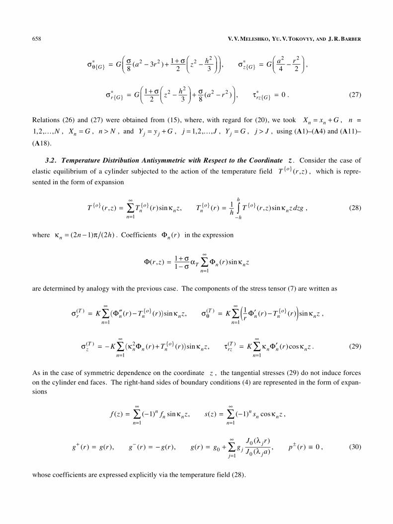
3.2. Temperature Distribution Antisymmetric with Respect to the Coordinate z . Consider the case of

elastic equilibrium of a cylinder subjected to the action of the temperature field T{o}(r, z) , which is repre-

sented in the form of expansion

T {o} (r, z) = Tn

{o} (r)sin�nz,n=1

�

� Tn{o} (r) = 1

hT {o} (r, z)sin�nz dz

�h

h

� g , (28)

where �n = (2n �1)�/(2h) . Coefficients �n (r) in the expression

�(r, z) = 1+ �1� � �T �n (r)sin�nz

n=1

�

�

are determined by analogy with the previous case. The components of the stress tensor (7) are written as

�r

(T ) = K ( ���n (r) � Tn{o} (r))sin�nz

n=1

, ��(T ) = K 1

r��n (r) � Tn

{o} (r)( )sin�nzn=1

,

� z

(T ) = �K (�n2�n (r)+ Tn

{o} (r))sin�nzn=1

, �rz(T ) = K �n ��n (r)cos�nz

n=1

. (29)

As in the case of symmetric dependence on the coordinate z , the tangential stresses (29) do not induce forces on the cylinder end faces. The right-hand sides of boundary conditions (4) are represented in the form of expan-sions

f (z) = (�1)n fn sin�nz,n=1

�

� s(z) = (�1)n sn cos�nzn=1

�

� ,

g+ (r) = g(r), g� (r) = � g(r), g(r) = g0 + g j

J0 (� j r)

J0 (� ja),

j=1

�

� p± (r) � 0 , (30)

whose coefficients are expressed explicitly via the temperature field (28).

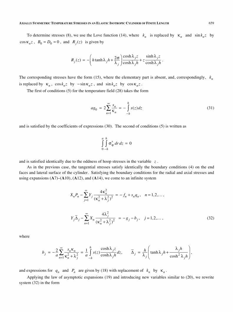
AXIALLY SYMMETRIC TEMPERATURE STRESSES IN AN ELASTIC ISOTROPIC CYLINDER OF FINITE LENGTH 659

To determine stresses (8), we use the Love function (14), where kn is replaced by �n and sin knz by

cos�nz , B0 = D0 = 0 , and Rj (z) is given by

Rj (z) = � h tanh� jh +2�� j

���

�

cosh� j z

cosh� jh+ z

sinh� j z

cosh� jh.

The corresponding stresses have the form (15), where the elementary part is absent, and, correspondingly, kn

is replaced by �n , cos knz by � sin�nz , and sin knz by cos�nz .

The first of conditions (5) for the temperature field (28) takes the form

ag0 = 2sn

�nn=1

�

� = � s(z)dz�h

h

� (31)

and is satisfied by the coefficients of expressions (30). The second of conditions (5) is written as

���

�h

h

�0

a

� dr dz = 0

and is satisfied identically due to the oddness of hoop stresses in the variable z . As in the previous case, the tangential stresses satisfy identically the boundary conditions (4) on the end

faces and lateral surface of the cylinder. Satisfying the boundary conditions for the radial and axial stresses and using expansions (�7)–(�10), (�12), and (�14), we come to an infinite system

XnPn � Yj4�n

2

(�n2 + � j

2 )2j=1

�

� = � fn + snqn , n = 1,2,… ,

Yj� j � Xn

4� j2

(�n2 + � j

2 )2n=1

�

� = � g j � bj , j = 1,2,… , (32)

where

bj = � 2a

sn�n

�n2 + � j

2n=1

�

� = 1a

s(z)cosh� j z

cosh� jhdz

�h

h

� , � j = h� j

tanh� jh +� jh

cosh2 � jh

�

�

�

� ,

and expressions for qn and Pn are given by (18) with replacement of kn by �n .

Applying the law of asymptotic expansions (19) and introducing new variables similar to (20), we rewrite system (32) in the form

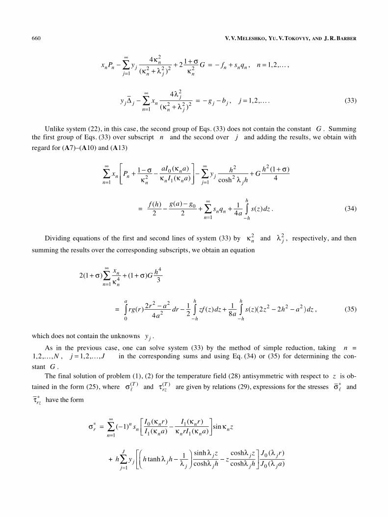
660 V. V. MELESHKO, YU. V. TOKOVYY, AND J. R. BARBER

xnPn � y j4�n

2

(�n2 + � j

2 )2j=1

�

� + 2 1+ ��n

2G = � fn + snqn , n = 1,2,… ,

y j� j � xn

4� j2

(�n2 + � j

2 )2n=1

�

� = � g j � bj , j = 1,2,… . (33)

Unlike system (22), in this case, the second group of Eqs. (33) does not contain the constant G . Summing the first group of Eqs. (33) over subscript n and the second over j and adding the results, we obtain with

regard for (�7)–(�10) and (�13)

xn Pn +1� ��n

2�

aI0 (�na)�n I1(�na)

��

�

� n=1

�

� � y jh2

cosh2 � jhj=1

�

� + Gh2 (1+ �)

4

= f (h)

2�

g(a) � g02

+ snqnn=1

�

� + 14a

s(z)dz�h

h

� . (34)

Dividing equations of the first and second lines of system (33) by �n2 and � j

2 , respectively, and then

summing the results over the corresponding subscripts, we obtain an equation

2(1+ �)xn

�n4+ (1+ �)G h4

3n=1

�

�

=

rg(r) 2r2 � a2

4a2dr

0

a

� � 12

zf (z)dz�h

h

� + 18a

s(z)(2z2 � 2h2 � a2 )dz�h

h

� , (35)

which does not contain the unknowns y j .

As in the previous case, one can solve system (33) by the method of simple reduction, taking n =

1,2,…, N , j = 1,2,…, J in the corresponding sums and using Eq. (34) or (35) for determining the con-

stant G . The final solution of problem (1), (2) for the temperature field (28) antisymmetric with respect to z is ob-

tained in the form (25), where ��(T ) and �rz

(T ) are given by relations (29), expressions for the stresses ��� and

�rz� have the form

�r� = (�1)n sn

I0 (�nr)I1(�na)

�I1(�nr)

�nrI1(�na)�

�� sin�nz

n=1

�

�

+ h y j h tanh� jh �1� j

���

��

sinh� j z

cosh� jh� z

cosh� j z

cosh� jh

�

�

��

j=1

J

�J0 (� j r)

J0 (� ja)

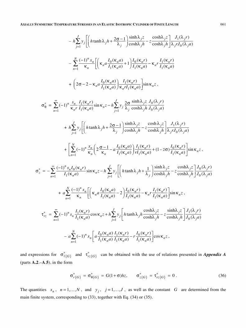
AXIALLY SYMMETRIC TEMPERATURE STRESSES IN AN ELASTIC ISOTROPIC CYLINDER OF FINITE LENGTH 661

– h y j h tanh� jh +2� �1� j

���

� �

sinh� j z

cosh� jh� z

cosh� j z

cosh� jh

�

�

��

j=1

J

�J1(� j r)

� j rJ0 (� ja)

– (�1)n xn

�n�na

I0 (�na)I1(�na)

+1���

��

I0 (�nr)I1(�na)

� �nrI1(�nr)I1(�na)

�n=1

N

�

+ 2� � 2 � �naI0 (�na)I1(�na)

���

�

I1(�nr)�nrI1(�na)

�� sin�nz ,

��� = (�1)n sn

�nrI1(�nr)I1(�na)

sin�nzn=1

� h y j2�� j

sinh� j z

cosh� jhj=1

J

J0 (� j r)

J0 (� ja)

+ h y j h tanh� jh +2� �1� j

���

� �

sinh� j z

cosh� jh� z

cosh� j z

cosh� jh

�

�

��

j=1

J

�J1(� j r)

� j rJ0 (� ja)

+ (�1)n xn

�n2 � �1

�n� a

I0 (�na)I1(�na)

���

� �

n=1

N

� I1(�nr)rI1(�na)

+ (1� 2�)I0 (�nr)I1(�na)

�

�

��sin�nz ,

� z� = �

(�1)n sn I0 (�nr)I1(�na)

sin�nz � hn=1

�

� y j h tanh� jh +1� j

�

���

sinh� j z

cosh� jh� z

cosh� j z

cosh� jh�

�

�

��

j=1

J

�J0 (� j r)

J0 (� ja)

+ a(�1)n xn

�nn=1

N

� �naI0 (�na)I1(�na)

� 2���

��

I0 (�nr)I1(�na)

� �nrI1(�nr)I1(�na)

�

���sin�nz ,

�rz� = (�1)n sn

I1(�nr)I1(�na)

n=1

�

� cos�nz + h y j h tanh� jhcosh� j z

cosh� jh� z

sinh� j z

cosh� jh

�

�

��

J1(� j r)

J0 (� ja)j=1

J

�

– a (�1)n xn aI0 (�na)I1(�na)

I1(�nr)I1(�na)

� rI0 (�nr)I1(�na)

���

�

cos�nzn=1

N

� ,

and expressions for ��{G}� and

�rz{G}� can be obtained with the use of relations presented in Appendix A

(parts �.2.–�.5), in the form

�r{G}� = ��{G}

� = G(1+ �)hz, � z{G}� = �rz{G}

� = 0 . (36)

The quantities xn , n = 1,…, N , and y j , j = 1,…, J , as well as the constant G are determined from the

main finite system, corresponding to (33), together with Eq. (34) or (35).

662 V. V. MELESHKO, YU. V. TOKOVYY, AND J. R. BARBER

Table 1

z N = J = 3 [6, Table 9, p. 107], [7, Table 20, p. 238]

0.0 –6.533 –6.532

0.1 –6.443 –6.457

0.2 –6.180 –6.211

0.3 –5.766 –5.807

0.4 –5.197 –5.218

0.5 –4.447 –4.454

0.6 –3.494 –3.508

0.7 –2.379 –2.426

0.8 –1.245 –1.284

0.9 –0.330 –0.326

1.0 0.059 0.200

4. Examples of Calculations

The basic problem for checking the methods of solution of the problems of thermoelasticity for a finite cyl-inder is the determination of thermal stresses caused by a temperature field that is independent of the axial coor-dinate z and is a polynomial of the radial coordinate r . In particular, the typical example of only radial de-pendence of the temperature field

T = T0r2/a2 , T0 = const (37)

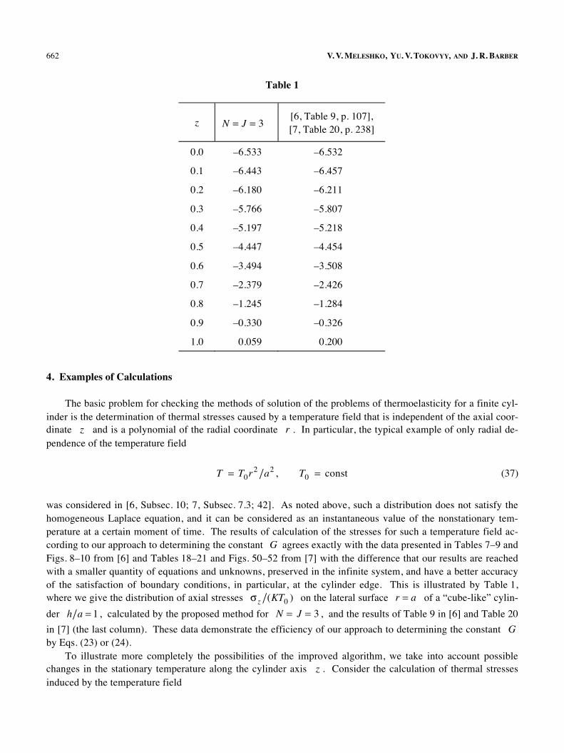
was considered in [6, Subsec. 10; 7, Subsec. 7.3; 42]. As noted above, such a distribution does not satisfy the homogeneous Laplace equation, and it can be considered as an instantaneous value of the nonstationary tem-perature at a certain moment of time. The results of calculation of the stresses for such a temperature field ac-cording to our approach to determining the constant G agrees exactly with the data presented in Tables 7–9 and Figs. 8–10 from [6] and Tables 18–21 and Figs. 50–52 from [7] with the difference that our results are reached with a smaller quantity of equations and unknowns, preserved in the infinite system, and have a better accuracy of the satisfaction of boundary conditions, in particular, at the cylinder edge. This is illustrated by Table 1, where we give the distribution of axial stresses � z /(KT0 ) on the lateral surface r = a of a “cube-like” cylin-

der h/a = 1, calculated by the proposed method for N = J = 3 , and the results of Table 9 in [6] and Table 20

in [7] (the last column). These data demonstrate the efficiency of our approach to determining the constant G by Eqs. (23) or (24).

To illustrate more completely the possibilities of the improved algorithm, we take into account possible changes in the stationary temperature along the cylinder axis z . Consider the calculation of thermal stresses induced by the temperature field

AXIALLY SYMMETRIC TEMPERATURE STRESSES IN AN ELASTIC ISOTROPIC CYLINDER OF FINITE LENGTH 663

T (r, z) = T0 r2 � a2

2� 2 z2 � h2

3���

���+ z2 � 3r2

2���

���

z�

� �, T0 = const , (38)

which represents a harmonic function and, according to (9), can be decomposed into the sum of components even and odd in the variable z :

T {e} (r, z) = T0 r2 � a2

2� 2 z2 � h2

3���

���

�

� �, T {o} (r, z) = T0 z2 � 3r2

2���

���

z . (39)

We normalize all components of the stresses by a constant multiplier KT0 , which is omitted in what follows in

the interest of brevity. We take � = 1/3 in these calculations.

Stresses (12) for the temperature field T{e} , given by relation (39), are written in simple form:

�r(T ) = a2 � r2

4+ 2z2 � 2h2

3, ��

(T ) = a2 � 3r2

4+ 2z2 � 2h2

3,

� z(T ) = a2 � 2r2

2, �rz

(T ) = 0 ,

as also stresses (29) for T{o} :

�r

(T ) = ��(T ) = 3z

2(r2 + h2 � z2 ) ,

� z

(T ) = z(z2 � 3h2 ), �rz(T ) = 3a

2(h2 � z2 ) .

In the case of temperature distribution symmetric with respect to z , the coefficients of boundary conditions (13) are written in the form

f0 = g0 = sn = 0, fn = � 8kn

2, g j = 4

� j2

, (40)

and in the case of antisymmetric distribution, the corresponding functions (30) have coefficients

fn = 6�n

2h2 � 3

�n4h

� 3a2

�n2h

, sn = 6a�n

3h, g0 = 2h3, g j = 0 . (41)

Note that, in the case of temperature field T{e} , given by the first relation (39), the integral conditions (5) are

satisfied due to the equality of the corresponding coefficients (40) to zero, and in the case of T{o} , assigned by

the second relation (39), equality (31) for coefficients (41) takes place.

664 V. V. MELESHKO, YU. V. TOKOVYY, AND J. R. BARBER

Fig. 1

Fig. 2

The main criterion for assessing the accuracy of the calculated stress field (15) is the satisfaction of the cor-

responding boundary conditions by the normal stresses �r� and � z

� , which is connected with the solution of

systems (22) and (33) for a finite quantity of terms in the corresponding sums. For this example, in the case of a

cylinder h/a = 1 and temperature field T{e} , the axial stresses � z

� satisfy the corresponding boundary con-

ditions (4), (13), and (40) to within 5% accuracy at N = J = 1 in system (22). If N = J = 2 , the error is about

2%, and if N = J = 3, it does not exceed 0.4%. For the radial stresses �r� , we have 1.4%, 0.3%, and 0.07%,

respectively. In the case of temperature field T{o} , the axial stresses � z

� satisfy the boundary conditions (4),

(30), and (41) to within 0.1% accuracy already at N = J = 1 in system (33), and the radial stresses to within 0.4% for the same values of N and J . With increase in the ratio h/a , the accuracy of satisfying the bound-

ary conditions becomes better because the influence of cylinder end faces decreases. These facts demonstrate the efficiency of our approach on the whole and, in particular, of the procedure of determining the asymptotic behavior of unknowns in the corresponding infinite systems on the basis of the law of asymptotic expan-sions (19). Therefore, in contrast to the algorithm of simple reduction, the approach considered here enables one to calculate efficiently the thermostressed state of a finite cylinder everywhere, including the points of its edges.

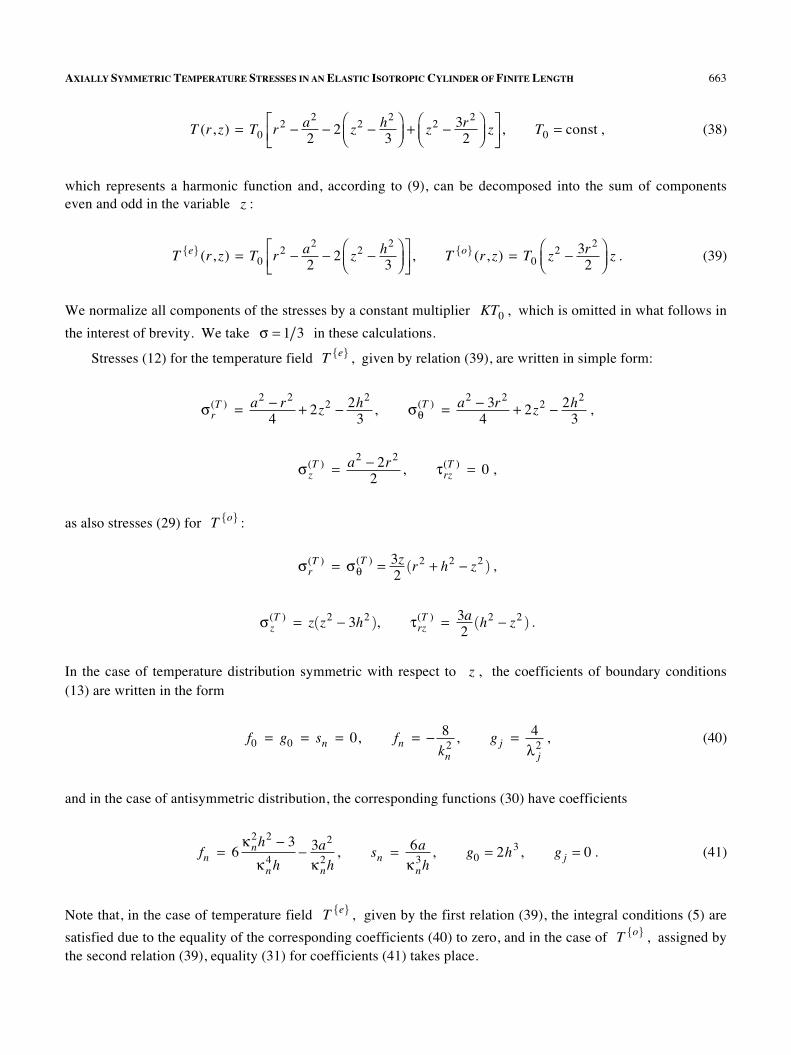
When the temperature field depends on the axial coordinate, the character of the stress distribution is af-fected. In Fig. 1, we show the distribution of axial stresses � z along the coordinate z on radii

r = 0, 0.5, 1.0 , calculated for the temperature field (38) in cylinder h = a = 1 at N = J = 3 in systems (22)

AXIALLY SYMMETRIC TEMPERATURE STRESSES IN AN ELASTIC ISOTROPIC CYLINDER OF FINITE LENGTH 665

and (33). These stresses reach their maximum on the cylinder lateral surface, and, unlike the case of temperature field (37), this maximum is situated not in the central cross section z = 0 , but is shifted to the end face z =

� h , which is caused by the contribution of antisymmetric component T{o} , given by the second relation (39),

to the temperature field (38). Note that these stresses are compressive near the cylinder axis but become tensile over almost the entire cylinder length as the lateral surface r = a is approached, decaying near the end faces. This feature is caused by the fact that the stresses � z satisfy boundary conditions on the end faces z = ±h ,

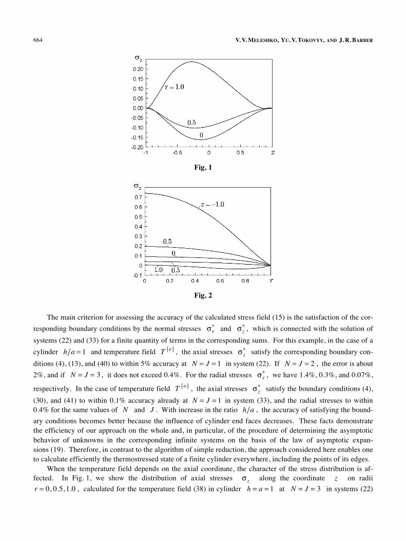
including edges (curve r = 1 ). Figure 2 illustrates the distribution of radial stresses �r along the coordinate r in cross sections z = 0,

± 0.5 , ±1.0 , calculated for the same parameters h = a = 1 and N = J = 3. Comparing curves for the positive

and negative values of z , we detect the influence of dependence of the temperature field on z, as a result of which the maximal values of radial stresses are reached on the end face z = �h on the cylinder axis r = 0 .

The stresses �r satisfy homogeneous conditions on the lateral surface in every cross section z = const , in-

cluding edges (curves z = ±1 ).

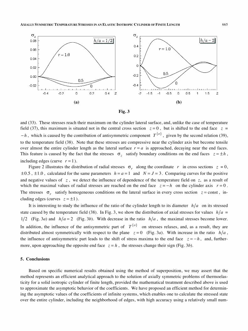
It is interesting to study the influence of the ratio of the cylinder length to its diameter h/a on its stressed

state caused by the temperature field (38). In Fig. 3, we show the distribution of axial stresses for values h/a =

1/2 (Fig. 3a) and h/a = 2 (Fig. 3b). With decrease in the ratio h/a , the maximal stresses become lower.

In addition, the influence of the antisymmetric part of T{o} on stresses relaxes, and, as a result, they are

distributed almost symmetrically with respect to the plane z = 0 (Fig. 3a). With increase in the ratio h/a , the influence of antisymmetric part leads to the shift of stress maxima to the end face z = �h , and, further-

more, upon approaching the opposite end face z = h , the stresses change their sign (Fig. 3b).

5. Conclusions

Based on specific numerical results obtained using the method of superposition, we may assert that the method represents an efficient analytical approach to the solution of axially symmetric problems of thermoelas-ticity for a solid isotropic cylinder of finite length, provided the mathematical treatment described above is used to approximate the asymptotic behavior of the coefficients. We have proposed an efficient method for determin-ing the asymptotic values of the coefficients of infinite systems, which enables one to calculate the stressed state over the entire cylinder, including the neighborhood of edges, with high accuracy using a relatively small num-

(a) (b)

Fig. 3

666 V. V. MELESHKO, YU. V. TOKOVYY, AND J. R. BARBER

ber of equations and unknowns in the main systems. We have revealed the characteristic features of infinite sys-tem in the case of stressed state antisymmetric with respect to the axial coordinate. We have also shown that the presence of components (27) and (36) in the complete expressions for stresses is important for adequate calcula-tion of the stressed state near the cylinder edges. Although the algebraic transformations can seem somewhat sophisticated, the final relations are quite simple for practical calculations. The proposed method of solution of infinite systems, obtained from considering the axially symmetric problems of thermoelasticity for cylinders, provides both a reliable way for the construction of an accurate engineering solution and a series of interesting mathematical results.

Appendix �

�.1. Expansion of functions into Fourier series in the complete system of trigonometric functions 1, cos knz , sin knz , where kn = n�/h , n = 1,2,… :

z2 � h2

3=

4(�1)n

kn2

cos knzn=1

�

� , (�1)

cosh�zsinh�h

� 1�h

=2�(�1)n

h(kn2 + �2 )

cos knzn=1

�

� , (�2)

z sinh�zsinh�h

+ 1� � h coth�h( ) cosh�z

sinh�h=

4(�1)n kn2

h(kn2 + �2 )2

cos knzn=1

�

� , (�3)

z cosh�zsinh�h

� h coth�h sinh�zsinh�h

=4�(�1)n kn

h(kn2 + �2 )2

sin knzn=1

�

� , (�4)

z2= �

(�1)n

knsin knz

n=1

�

� , (�5)

z(z2 � h2 )

12=

(�1)n

kn3

sin knzn=1

�

� . (�6)

�.2. Expansion of functions into Fourier series in the complete systems of trigonometric functions cos�nz , sin�nz , where �n = (2n �1)�/(2h) , n = 1,2,… :

z cosh�zcosh�h

� h tanh�h � 1�( ) sinh�z

cosh�h=

(�1)n+1�n2

h(�n2 + �2 )2

sin�nzn=1

�

� , (�7)

zh2

=(�1)n+1

�n2

sin�nzn=1

�

� , (�8)

AXIALLY SYMMETRIC TEMPERATURE STRESSES IN AN ELASTIC ISOTROPIC CYLINDER OF FINITE LENGTH 667

sinh�zcosh�h

=(�1)n+1 2�h(�n

2 + �2 )sin�nz

n=1

�

� , (�9)

cosh�zcosh�h

=(�1)n+1�n

h(�n2 + �2 )

cos�nzn=1

�

� . (�10)

�.3. Expansion of functions into Fourier–Bessel series in the complete system of functions 1, J0 (� j r) ,

where J1(� ja) = 0 :

r2

2� a2

4= 2

� j2

J0 (� j r)

J0 (� ja)j=1

�

� , (�11)

aI0 (kr)I1(ka)

� 2k= 2k

� j2 + k2

J0 (� j r)

J0 (� ja)j=1

�

� , (�12)

I0 (ka)I1(ka)

I0 (kr)I1(ka)

� ra

I1(kr)I1(ka)

� 4k2a2

= 4k2

a2 (� j2 + k2 )2

J0 (� j r)

J0 (� ja)j=1

�

� , (�13)

ra

I1(kr)I1(ka)

+ 2ka

�I0 (ka)I1(ka)

���

���

I0 (kr)I1(ka)

=4� j

2

a2 (� j2 + k2 )2

J0 (� j r)

J0 (� ja)j=1

�

� . (�14)

�.4. Expansion into Dini series in the complete system of functions J1(� j r) , where J1(� ja) = 0 :

r = � 2� j

J1(� j r)

J0 (� ja)j=1

�

� , (�15)

r(r2 � a2 )

16= 1

� j3

J1(� j r)

J0 (� ja)j=1

�

� , (�16)

aI1(kr)I1(ka)

= �2� j

� j2 + k2

J1(� j r)

J0 (� ja)j=1

�

� , (�17)

ra

I0 (kr)I1(ka)

�I0 (ka)I1(ka)

I1(kr)I1(ka)

=2� j k

a2 (� j2 + k2 )2

J1(� j r)

J0 (� ja)j=1

�

� . (�18)

�.5. Values of infinite sums:

4kn

2

(�2 + kn2 )2

= h� coth�h � �h

sinh2 �h

�

��n=1

�

� , (�19)

668 V. V. MELESHKO, YU. V. TOKOVYY, AND J. R. BARBER

1kn

2= h2

6k=1

�

� , (�20)

4� j

2

(k2 + � j2 )2

= a2 1�I0

2 (ka)

I12 (ka)

�

���

��j=1

�

� + 2ak

I0 (ka)I1(ka)

, (�21)

1� j

2= a2

8j=1

�

� , (�22)

1(kn

2 + �2 )2=

n=1

�

� h4�3

coth�h + �hsinh2 �h

� 2�h

�

��

, (�23)

1kn

4= h4

90n=1

�

� , (�24)

1(k2 + � j

2 )2= a2

4k2

I02 (ka)

I12 (ka)

�1�

���

��j=1

�

� � 1kn

4, (�25)

1� j

4= a4

192j=1

�

� , (�26)

1(�n

2 + �2 )2= h

4�3tanh�h � �h

cosh2 �h

��

���

n=1

�

� , (�27)

1�n

4= h4

6n=1

�

� . (�28)

REFERENCES

1. V. M. Vigak, Control of Temperature Stresses and Displacements [in Russian], Naukova Dumka, Kiev (1988). 2. V. M. Vihak and Yu. V. Tokovyy, “Exact solution of an axially symmetric problem of the theory of elasticity in stresses for a solid

cylinder of a certain length,” Prykl. Probl. Mekh. Mat., No. 1, 55–60 (2003). 3. I. I. Gol’denblatt, Analysis of Temperature Stresses in Nuclear Reactors [in Russian], Énergiya, Moscow (1962). 4. V. T. Grinchenko, “Stationary thermal stresses in a solid cylinder of finite length,” in: Thermal Stresses in Structural Elements

[in Russian], Issue 2 (1962), pp. 41–49. 5. V. T. Grinchenko, “Stressed state of a round thick disk in the field of centrifugal forces,” in: Proceedings of the IV All-Union Con-

ference on the Theory of Plates and Shells [in Russian], Izd. Akad. Nauk Arm. SSR, Yerevan (1964), pp. 423–430. 6. V. T. Grinchenko, Equilibrium and Steady-State Vibrations of Elastic Bodies of Finite Sizes [in Russian], Naukova Dumka, Kiev

(1978). 7. A. D. Kovalenko, Foundations of Thermoelasticity [in Russian], Naukova Dumka, Kiev (1970). 8. A. D. Kovalenko, Thermoelasticity [in Russian], Vyshcha Shkola, Kiev (1975).

AXIALLY SYMMETRIC TEMPERATURE STRESSES IN AN ELASTIC ISOTROPIC CYLINDER OF FINITE LENGTH 669

9. M. A. Koltunov, Yu. N. Vasil’ev, and V. A. Chernykh, Elasticity and Strength of Cylindrical Bodies [in Russian], Vysshaya Shkola, Moscow (1975).

10. B. G. Korenev, Problems of the Theory of Heat Conduction and Thermoelasticity [in Russian], Nauka, Moscow (1980). 11. B. M. Koyalovich, “A study of infinite systems of linear algebraic equations,” in: Transactions of the Steklov Physical-and-

Mathematical Institute [in Russian], Vol. 3 (1930), pp. 41–167. 12. N. N. Lebedev, Temperature Stresses in the Theory of Elasticity [in Russian], ONTI, Leningrad (1937). 13. V. M. Maizel’, Temperature Problem of the Theory of Elasticity [in Russian], Izd. Akad. Nauk Ukr. SSR, Kiev (1951). 14. V. V. Meleshko, “Thermal stresses in rectangular plates,” Mat. Met. Fiz.-Mekh. Polya, 48, No. 4, 140–164 (2005). 15. P. F. Papkovich, “General integral of thermal stresses (on the work ‘Thermal stresses in the theory of elasticity’ by N. N. Lebedev),”

Prikl. Mat. Mekh., 1, No. 2, 245–246 (1937). 16. P. F. Papkovich, Theory of Elasticity [in Russian], Oborongiz, Leningrad (1939). 17. Ya. S. Podstrigach and Yu. M. Kolyano, Unsteady-State Temperature Fields and Stresses in Thin Plates [in Russian], Naukova

Dumka, Kiev (1972). 18. K. V. Solyanik-Krassa, Axially Symmetric Problem of the Theory of Elasticity [in Russian], Stroiizdat, Moscow (1987). 19. S. P. Timoshenko, A Course in the Theory of Elasticity [in Russian], Naukova Dumka, Kiev (1972. 20. I. I. Fedik, V. S. Kolesov, and V. N. Mikhailov, Temperature Fields and Thermal Stresses in Nuclear Reactors [in Russian], Énergo-

atomizdat, Moscow (1985). 21. V. S. Arpaci, “Steady axially symmetric three-dimensional thermoelastic stresses in fuel rods,” Nucl. Eng. Des., 80, 301–307 (1984). 22. J. R. Barber, Elasticity, Springer, New York (2010). 23. B. A. Boley and J. H. Weiner, Theory of Thermal Stresses, Wiley, New York (1960). 24. D. Burgreen, Elements of Thermal Stress Analysis, C.P. Press, Jamaica (1971). 25. J. M. C. Duhamel, “Mémoire sur le calcul des actions moléculaires développées par les changements de la température dans les

corps solides,” Mém. Acad. Sci. Savans Étrang, 5, 440–498 (1838). 26. B. E. Gatewood, Thermal Stresses, with Applications to Airplanes, Missiles, Turbines and Nuclear Reactors, McGraw-Hill, New

York (1957). 27. J. N. Goodier, “On the integration of the thermo-elastic equations,” Philos. Mag. (Ser. 7), 23, 1017–1032 (1937). 28. R. B. Hetnarski and M. R. Eslami, Thermal Stresses. Advanced Theory and Applications, Springer, Dordrecht (2009). 29. G. Horvay, I. Giaver, and J. A. Mirabal, “Thermal stresses in a heat-generating cylinder: The variational solution of a boundary layer

problem in three-dimensional elasticity,” Ing.-Archiv, 27, 179–194 (1959). 30. D. J. Johns, Thermal Stress Analysis, Pergamon, Oxford (1965). 31. A. D. Kovalenko, Thermoelasticity. Basic Theory and Applications, Wolters-Noordhoff, Groningen (1969). 32. A. E. H. Love, A Treatise on the Mathematical Theory of Elasticity, 4th edition, Cambridge Univ. Press, Cambridge (1927). 33. J. R. Matthews, “Thermal stress in a finite heat generating cylinder,” Nucl. Eng. Des., 12, 291–296 (1970). 34. E. Melan and H. Parkus, Wärmespannungen Infolge Stationärer Temperaturfelder, Springer, Wien (1953). 35. V. V. Meleshko, “Equilibrium of an elastic finite cylinder: Filon’s problem revisited,” J. Eng. Math., 46, 355–376 (2003). 36. K. E. Neumann, “Die Gesetze der Doppelbrechung des Lichts in comprimirten oder ungleichförmig erwärmten unkrystallinischen

Körpern,“ Abhandl. Königl. Akad. Wissen. Berlin, No. 2, 1–254 (1841). 37. N. Noda, R. B. Hetnarski, and Y. Tanigawa, Thermal Stresses, Taylor & Francis, New York (2003). 38. W. Nowacki, Thermoelasticity, Pergamon, London (1962). 39. H. Parkus, Instationärer Wärmespannungen, Springer, Wien (1959). 40. M. H. Sadd, Elasticity: Theory, Applications, and Numerics, Academic, Burlington (2009). 41. K. T. Sundara Raja Iyengar and K. Chandrashekhara, “Thermal stresses in a finite solid cylinder due to an axisymmetric temperature

field at the end surface,” Nucl. Eng. Des., 3, 382–393 (1966). 42. K. T. Sundara Raja Iyengar and K. Chandrashekhara, “Thermal stresses in a finite solid cylinder due to steady temperature variation

along the curved and end surfaces,” Int. J. Eng. Sci., 5, 393–413 (1967). 43. S. Timoshenko, Theory of Elasticity, McGraw-Hill, New York (1934). 44. S. P. Timoshenko and J. N. Goodier, Theory of Elasticity, McGraw-Hill, New York (1970). 45. R. A. Valentin and J. J. Carey, “Thermal stresses and displacements in finite, heat-generating cylinders,” Nucl. Eng. Des., 12, 277–

290 (1970).