LNLS is part of the CNPEM an organization certified by the Ministry of Science, Technology, Innovation and

Communication (MCTIC).

Address: Rua Giuseppe Máximo Scolfaro, 10.000 - Polo II de Alta Tecnologia - Caixa Postal 6192 - 13083-970

Campinas/SP

Telephone: +55.19.3512.1010 | www.lnls.cnpem.br

Avizo Guide A quick start

X-Ray Imaging Beamline (IMX)

Julho/2017

2

Documentation History

Date Revision Description Author

31/07/2016 1 Version based on Avizo 9.1 Nathaly L. Archilha

08/08/2017 2 Update to Avizo 9.3 Nathaly L. Archilha

3

Summary

1. How to create a 3D volume of your data............................................................................... 4

Opening your data ............................................................................................................. 4

Adding and checking the ortho slices................................................................................ 9

Adding a scale bar ........................................................................................................... 13

Changing the background ................................................................................................ 14

2. Filtering and Segmentation tools ......................................................................................... 19

Filtering the image .......................................................................................................... 19

Segmenting the image ..................................................................................................... 22

I. Pick and Move ............................................................................................................. 22

II. Brush tool .................................................................................................................... 24

III. Lasso tool (2D and 3D) ........................................................................................... 26

IV. Magic Wand tool ..................................................................................................... 27

V. Propagation Contour ................................................................................................... 29

VI. Blow Tool ................................................................................................................ 30

VII. Threshold tool ......................................................................................................... 31

VIII. TopHat tool ............................................................................................................. 36

IX. Watershed ................................................................................................................ 38

Special applications using segmentation tools ................................................................ 38

I. Removing the background using watershed tool ........................................................ 38

II. Segmenting your image using a mask ......................................................................... 45

3. Quantification ...................................................................................................................... 49

Volume of a label ............................................................................................................ 49

Separate tool .................................................................................................................... 51

Label analysis .................................................................................................................. 55

Connectivity .................................................................................................................... 57

4

1. How to create a 3D volume of your data

Opening your data

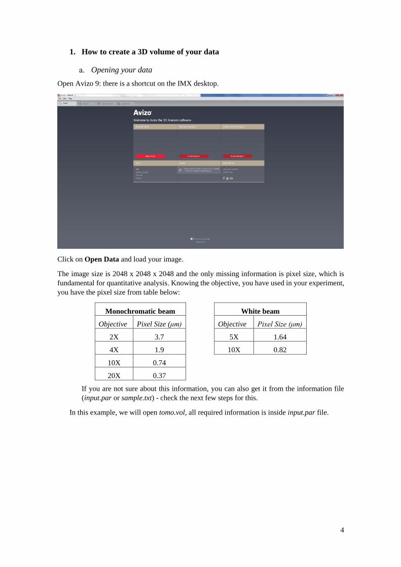
Open Avizo 9: there is a shortcut on the IMX desktop.

Click on Open Data and load your image.

The image size is 2048 x 2048 x 2048 and the only missing information is pixel size, which is

fundamental for quantitative analysis. Knowing the objective, you have used in your experiment,

you have the pixel size from table below:

Monochromatic beam

White beam

Objective Pixel Size (μm)

Objective Pixel Size (μm)

2X 3.7

5X 1.64

4X 1.9

10X 0.82

10X 0.74

20X 0.37

If you are not sure about this information, you can also get it from the information file

(input.par or sample.txt) - check the next few steps for this.

In this example, we will open tomo.vol, all required information is inside input.par file.

5

First, open the information file (input.par), using Notepad++ or gedit.

6

A new window will open. Here, you will find information regarding X and Y dimensions of your

image (red box), Z dimension is always 2048, if all slices were reconstructed (green arrow). Pixel

size (red arrow) is always shown in micrometers. Note: If you cropped your image, use the new

dimensions.

7

Then, open the volume file.

The Out-of-Core Data window will open; select Read complete volume into memory.

8

The Raw Data Parameters window will open and you have to fill it with the following

information:

- Data type: the output of the reconstruction is 32-bit; however, it is possible to transform

the image into 16- or 8-bit using ImageJ (see Section Erro! Fonte de referência não

encontrada.).

- Dimensions: you will find this in the information file (input.par) or if you cropped your

image, this information will be at the file name.

After adding these parameters, the Header value (red arrow) should be zero, as it

subtracts the file size of the requested size. If some information is wrong, the Header

will be different of zero – double check the information you added before you load the

image.

- Voxel size: also defined in the information file. You will find just two values, but it is the

same for the three axes, as the voxel is actually a cube.

9

Click OK and your image will be loaded. Depending on its size, it can take a couple of minutes!

At this point, it is very likely that the software requests the voxel size unit – choose micrometers.

If Avizo doesn´t request this right now, it is still possible to change it later.

This is an example of a toothpick.

Adding and checking the ortho slices

The image above shows an ortho slice of a toothpick sample. This view is automatically loaded

when you open a new image. To add more ortho slices, you have to click on your raw image (red

arrow) and then click on Ortho Slice (red box). Not all commands will be available as Ortho

Slice was. For these cases, you will need to open the dialog box (yellow box), by right clicking

the raw image. You can either look for all the options, by opening each folder (black box), or

write the command (i.e. ortho slice) at the search place (blue arrow).

Create two more ortho slices (red box). They will have the same orientation as the first Ortho

slice. For another view of your sample, click on Ortho Slice 2 and its Properties (green box) will

10

appear. Change its orientation to xz (blue box) and an orange line will appear in your image

(orange arrow).

Make the same for Ortho slice 3, but choose orientation yz for a complete view of your image.

To rotate the sample, click on the hand icon (red arrow), then click on the toothpick image and

drag the mouse.

You´ll see an image like the following one. If you want to change perspective, click on the

perspective icon (red arrow).

11

The new image is slightly different.

Next step is to create the 3D volume rendering of your sample. You can right click on the raw

image and look for Volume Rendering (red box) or you can click on the Volume Rendering button

(red arrow).

12

The result is the following image. If the image you create is not satisfactory, try to change the

threshold of your colormap (red arrows) until you find the best representation of your sample.

You can hide the ortho slices and show only the volume rendering of your sample. Just click on

the orange box in the raw image and it will turn it to gray (red arrow).

13

Adding a scale bar

To add a scale bar, you just need to click on Scalebars (red arrow) or search this in the searching

area (orange arrow)

A scale bar will appear on the left corner of your image. There are many options to edit it, some

of them are:

1) X and Y spatial positions (blue box).

2) X and Y sizes (red box).

3) X and Y frames (pink box): you enable or disable the axis.

4) Units (yellow box): if this box is unavailable/locked (not the case here), Avizo already

knows the units (i.e. you had included this information when you loaded your data).

Suggestion: for quantitative analysis, always include this information prior to your

analysis (Section d shows how to change this).

5) X and Y color and width, font color and type (green box).

14

Changing the background

The default gray background is not appropriate for publications and reports. To change this, go

to View Background.

Change color 1 to white and click on uniform. If the scale bar is white, it will disappear.

15

You simply need to click on Scalebars and change its color.

To correct the units, click on Edit Preferences.

16

Then, click on Units tab and click on Spatial information only (red arrow).

Unclick Lock display units on working units. Avizo working unit is meter, which is huge

comparing to our scale.

17

Click on Display unit and change Coordinates (red arrow) to an appropriated unit (normally

micrometer).

The final image is showed below.

18

To check or include the pixel size, you can click on Crop editor and check the red box. If it is

wrong, you can update these values.

19

2. Filtering and Segmentation tools

Even the best measurement and the most robust reconstruction method generate an image with a

noise. From this image, quantitative and qualitative information can be obtained. Prior to image

analysis, it is very common to take advantage of filters to improve the image quality and,

consequently, facilitate the post processing. The main goal of filtering an image is to remove noise

and this process consists on an image transformation, where the new image is obtained by

neighborhood operations. The next step is the image segmentation, which is the partitioning of an

image (R) into regions (R1, R2, R3,…, Rn) that are homogeneous with respect to some

characteristic, for example, intensity or texture. The idea is to study each label separately from

the others.

See below some filtering and segmentation tools available in Avizo.

Filtering the image

Load your image.

Using the Filter sandbox tool, you can test all the filters on a small piece of your image (little

square in the image bellow). It is useful to help you to decide which filter is the best one for your

case, in a very fast way.

20

Zoon in the image and move the square to a desirable area.

Click on Filter Sandbox (light blue) and its properties will be available. You can see that many

different filters are available (red arrow).

21

Choose the filter you want to test (in this case, it is Non Local Means). As this filter is very robust,

it can take a while to apply to your image. You will see a red bar on the bottom of your screen,

showing its progression.

The filtered image is inside the box.

22

You can make the same procedure to test the other filters. Once you have a decision, you can

apply the filter to the whole image by pressing Apply (red arrow).

Segmenting the image

To access the Segmentation menu, right click on the image to be segmented (normally it is the

filtered image) and type Edit new label field. On its properties menu, you will see many available

tools for segmentation. All of them are described below.

I. Pick and Move

This tool (red arrow) is ideal to select an unconnected segmented area of your image and move it

to another label. In the image below, the segmented area is shown in yellow. As an example, let’s

move one region that was wrongly assigned as pore space (black arrow), to the Matrix label.

23

Using Pick and Move, click on the region you want to select. This is a 3D selection, so check the

3D volume to be sure that you really want to move the whole selection to another label.

Click on the label that you want this region to be moved (in this case, Matrix) and then click add

(+). This region now is part of the Matrix label. See the final segmentation below, where the

matrix is represented by the purple color and the pore space is in yellow. To show or hide a

determined label, click on the small eye (2D or 3D), next to the name of the label (red arrow).

You can also check the label color and modify, by double clicking on the color box (green arrow).

24

II. Brush tool

If you have a connected piece of a label that you want to move to another label, you have to use

brush tool. For example, there are two regions (black arrows) that were wrongly assigned to

Background label, but it should be Matrix.

Go to Brush tool (red arrow), click on Background label (black arrow). Click on Select only

current material and, if necessary, Limited range only (if you know the threshold value that

contains the material you want to select) – if you do not select this, all the Background voxels

will be available for selection.

25

Select the region of interest. Attention, this is a 2D selection; you might change the slice number

to select a 3D region.

Add the selection to the correct label.

26

III. Lasso tool (2D and 3D)

This tool lets the user draw a closed contour, and selects all pixels within the contour. Some

options are available for 2D: free hand, ellipse and rectangle. Using free hand, you can use auto

trace, which will identify the edges of a certain area of the image.

If you want to use the 3D lasso, you have first to select a 2D area (right part of the image below)

and then check this is 3D (left part of the image). Note that you can only modify the selection

shape in the 2D image and, in the third direction (in this case, Z direction), the selection is

automatic.

27

IV. Magic Wand tool

Magic Wand is a region growing algorithm, which starts from a seed point and select all connected

voxels with a gray value in a given tolerance interval. The advantage of magic wand over

threshold tool is that it permits you to choose a single material/structure inside your image, i.e. if

you have other materials/structures with the same gray level, but it is not connected to the region

you want to segment, you will not select these voxels.

Click on magic wand tool (red arrow). In this example, the image is a toothpick with a micro gear

inside (bright region).

Click on the gear (red cross) and change the boundaries values (in this case, to 240 and 255).

28

Changing the boundaries values, you will change the result. In this example, 200 replaced 240

(red arrow), and the gear structure changed (blue arrows).

Choose the best values and add these voxels to a label field.

29

V. Propagation Contour

This tool is a fast-active contour. From a seed, which is created manually, a boundary front

evolves. Few parameters are available to be modified, as stop time and edge sensitivity. In this

example, we will use propagation contour to segment a specific pore of this soil sample. First,

you must create the seeds manually - check the figure below (red crosses).

Then, you click on Do it (red arrow), and the front will start evolving. After it finishes, you can

choose the best Time (green arrow) that represents the pore space.

30

VI. Blow Tool

This tool is useful to detect edges of a region and fill its interior, however it works only in 2D.

Click (and hold the button) on the area of interest. Drag the mouse, and the greater the distance

from the original point is, the more the contour grows. Release the button when the contour is in

a satisfactory place, like shown in the image bellow. The contour will grow in areas with

homogeneous grey values and will stop when it changes abruptly, i.e. when it finds an edge.

The tolerance (red arrow) controls how sharp the edge has to be in order to stop the contour

growing - the smaller this number is, the sharper the edge has to be. If this number is too large,

the contour will stop in weak edges.

After you release the mouse button, the area within the contour will be selected and you

can add to the desirable label.

31

VII. Threshold tool

The threshold tool separates the image into different regions according to the intensity values. To

separate the image using this tool, you just need to choose one or more threshold points in the

gray level histogram.

UPDATE (version 2): Avizo 9.3 has a new button inside the Segmentation Menu, named as

Select Masked Voxels (red arrow), which only appears if you are using the threshold tool. Now,

before adding a group of voxels to a specific label, you have to click on this button to select the

voxels and, only after this, add them to the desirable label.

32

As an example, we have an image of a carbonate rock. Clearly, it is possible to see two different

phases: matrix (light gray) and pores + background (dark gray).

Click on Threshold tool (red circle) and change the grey level values (in this case, to 82 and 255)

– this way, the rock matrix will be selected.

33

Each sample will require different numbers (threshold points). Once you have the best selection,

you have to apply for all slices (red arrow).

Add the selection to a label.

34

For a 3D view of your segmented image, click on the left small eye (red arrow) and check the top

left window.

Once you finish the segmentation, come back to Project window (red arrow). Now you have a

new image (.labels). This is your segmented image. Create an orthoslice and check the image.

35

You can create two more orthoslices and check all views.

You can also create a Volume rendering of your segmented image.

36

VIII. TopHat tool

This tool allows the detection of dark or white areas of the image. This tool is very useful to pick

small regions. As an example, this tool will be used to select the small pores of the following

image.

First, segment the big pores.

37

Then, the missing small pores will be segmented by TopHat tool. Click on Material5

label (red arrow), which represents everything that is not a big pore in this image. Since

all the unsegmented small pores are within this label, click on Select only current material

(green arrow). Choose between black or white – in this case, as the goal is to segment

pores, black is the best choice. Then, click on Compute Top Hat Image (blue arrow) – this

will be an available option at this point of the segmentation process.

Change the range (red arrow) to adjust the selection.

38

And add this region to the pore label (Material6, in this case).

IX. Watershed

Watershed is a robust segmentation toll and the idea consists of placing seeds in different regions

of the image and start growing this until it touches a global maximum (barrier) of the image,

which is determined by the image gradient.

This segmentation method is explained in Section c.I. (Removing the background using watershed

tool). Please, report to this section if you want to learn how to use this tool.

Special applications using segmentation tools

I. Removing the background using watershed tool

Remove the background of an image can be useful in many cases, e.g. you do not want to crop a

region of interest, either due to its heterogeneity or because you want to study its surface, or you

want to study the pore space of the sample - if the pore space is filled with air, there will be no

39

difference in grey level between the internal pores and the background. To remove the

background, follow the next steps.

First, load the image.

Apply a filter, if needed (in this case, NLM). Just be sure that the filter preserves the edges, which

are necessary to create the gradient image.

Click on Edit new label field and click on the full window (red arrow), for a better view.

40

Using threshold tool, select as much as you can of your sample. Do not select the background,

since this selection will be used as seeds.

Start growing (red arrow) the selection until you close all the internal pores (check all the slices,

if necessary, grow a little bit more the selection).

41

Add this selection to a new label (in this case, Material3).

Select (red arrow) the Exterior label and add this to a new label field (in this case, Material4).

42

Select Material3 (the selected area will turn red).

Start shrinking (red arrow) the region and stop when the red area is inside your sample.

43

Add the selection to the Inside label. Now the whole image is divided into three different labels:

Inside label has the seed of you sample (which also contains the internal pores); Material3

contains the border of the sample and Material4 has the seed for the background.

Delete Material3 (that represents the border) by pressing delete or clicking on the Remove the

selected material (red arrow).

44

All the voxels of this material will be moved to the Exterior label.

Go to watershed tool (red arrow), be sure that Inside and Material4 are marked (green arrow),

create a New gradient image (blue arrow) and then click on Apply and create a new label field

(yellow arrow).

The final result is showed bellow. The background is in yellow (Material4 label) and the sample

is in purple (Inside label). Check all slices and if you do not have a satisfactory result, you have

to restart the process taking more care with the seeds selection, growing and shrinking processes.

45

II. Segmenting your image using a mask

Section c.I showed how to separate the image of your sample from the background, i.e. how to

create a label (or mask) for each region. After this, it is possible to segment the sample using this

mask. It is very useful, especially when you want to segment the pore space, which has the same

gray level of the exterior (background).

For this example, let’s use the image of the previews section. The idea is to separate the pore

space from the matrix. For this, let’s will use the Watershed tool again (but you can use any other

segmentation tool).

Go to threshold tool (red arrow), click on Inside label (green arrow) and then, Select only current

material (yellow arrow). This way you are going to use the Threshold tool only on the selected

material, in this case, the purple region.

46

Select the seeds of the matrix. Make sure that there are no matrix seeds within the pore space.

Add this selection to a new material (in this case, Material5).

Click on Inside label (red arrow) again and create the pore space seeds using the threshold tool.

Move all the voxels within the Inside label to the Exterior label.

47

Go to Watershed Tool, be sure that Material4, Material5 and Material6 are selected, click Create

new gradient image and then, click on Apply and create a new label image.

The final result is shown below.

To check if the segmentation is good, you can compare the original and segmented image, side

by side. Go to Project, you will see that there are three new *.labels files. The last one is your

final segmented image – create an orthoslice for this. Click on Two Viewers (red arrow), and

choose the image you want to show by hiding/showing the orthoslice (green arrow).

48

49

3. Quantification

In this chapter, some possibilities of quantification of a segmented image will be shown. So, at

this point, it is very important to have a good segmentation of your image, otherwise, you won’t

have a trustworthy result.

Volume of a label

The image below shows a sandstone rock, filtered with the non-local means and segmented with

a combination of threshold and watershed.

First, move the background to the Exterior label, since this is not a region of interest, in this

example.

It is possible to rename the label, by double clicking on it. This way is easier to understand the

final results.

50

Go to Project and check the labeled image (*.labels), the black region represents the background

and the sample (with its pore space) is represented by both dark and light blue.

Use the Volume Fraction tool to obtain information of the volume of pores and matrix.

51

A table will appear with the volume fraction values (red arrow). Adding both of the values, you

see that it is not equal to 1 (i.e. 100%), just because the software also considers the background

as part of your image, but a simple rule of three can give you the proper fractions.

Separate tool

Separation is a tool to individualize regions of an image, which can be, for example, pores or

grains. Let’s keep the same image used in the previous example, but now, the idea is to transform

the pore space into many individual pores (the same can be done with the matrix). Move all the

labels to the exterior, except the one you want to individualize. In this case, Matrix label will be

moved to the exterior.

52

And only the pore space will be left.

Right click on the image and type Separate Objects.

53

The Properties window will open. This tool is very sensitive to the Marker value (which works

like a seed), so, it might be a good an idea to vary the marker and check the final result, to make

the best decision. For that, click on Auto-refresh (red arrow) and it will create a new file

(*.separate).

To make it easier to check the final result, click on the *.separate image and type Labeling. Now,

every pore will receive a different color.

54

Create an orthoslice for this new image and check the result. There is a repetition of colors, but it

does not mean necessarily that they are the same pore (somehow connected in 3D), it is more

likely due to the high amount of pores and the lack of enough different colors.

If you go back to the Separate Object and change the Marker Extend, you will see that the

separation changes. The above image was with Marker = 3 and the following image, Marker =

10. Choose the best marker for your case.

55

Label analysis

Label analysis is a tool that permits to quantify your image. In this example, we will use the last

image, showed below, to obtain few parameters from each pore. For that, right click on the image

and type Label Analysis.

Clicking on ‘…’ (red arrow), you will open all the possibilities of measurements and you will also

be able to create your own list of measurements.

56

Create your measure group (red arrow) and choose all the properties (from the list) you want to

measure.

Apply to your image and check the table with the results. Each pore is represented by a different

number (red arrow), and you have the selected measures from each one of them. You can also

export your table (green arrow).

57

And save this in different formats and work with your data in any other desirable software.

Connectivity

The final example of this guide is the connectivity tool, which will give you information of the

number of neighbors of each pore (i.e. coordination number of the pore). For that, you must use

the first segmentation of your pore space (before the separation) and use the Auto Skeleton tool.

It will create a new file (*.SptGraph) and to visualize the result, right click on this and type Spatial

Graph View. The result is shown below. Each single pore is represented by one segment and two

dots. The segment represents the pore body and the dots, either an end point (border) or a point

of connection to another pore.

58

If you click on the *.SptGraph file, you will open its Properties window. Go to the Table option

(red arrow) and click on Show and it will open the table with some information regarding the

skeletonization. There you can find information regarding the coordination number of each pore

and the size of the segment (pore body) in the three directions. Note: Z coord is always zero here

because there is just one slice loaded, but in a real 3D image, this number is always bigger than

this.