Algorithms

Dynamic Programming

LCS (Longest Common Subsequence)abcddebbdabaed

Opt (n ,m)={An=Bm1+Opt (n−1 ,m−1 )

An≠ Bmmax {Opt (n ,m−1 )Opt (n−1,m )

d 0 ¿ ¿ ¿ ¿b 0 ¿ ¿ ¿ ¿a 0 ¿ ¿ ¿ ¿ c 0 1 2 ¿ ¿ ¿b 0 1 1 ¿ ¿ ¿a 0 0 0 ¿ ¿ ¿ ϕ 0 0 0 0 0 0 0 0ϕ b c d a b c ¿ ¿ ¿ ¿ ¿ ¿ ¿ ¿ ¿ ¿ ¿ ¿ ¿ ¿ ¿ ¿ ¿ ¿ ¿ ¿ ¿ ¿ ¿ ¿ ¿ ¿ ¿ ¿ ¿ ¿ ¿ ¿ ¿ ¿ ¿

Ramsy TheoryErdes and Szekeresh proved that given a permutation of {1 ,…,n }, at least one increasing or decreasing substring exists with length ¿√n.

For example, observe the following permutation of {1 ,…,10 }:10581436279(1,1 ) (1,2 ) (2,2 ) (1,3 )…

The pairs present the number of the longest increasing substring and longest decreasing substring till that point (accordingly).Since every number raises the length of one of the substrings by one (either the increasing or decreasing) each lengths pair is uniqueDue to this fact, one of the numbers must be at least √n

Bandwidth ProblemThe bandwidth problem is an NP hard problem.

Definition: Given a symmetrical matrix, is there a way to switch the columns s.t. the "bandwidth" of the matrix is smaller than a number received as input.Another variant is to find the column switch that produces the smallest bandwidth.

The bandwidth of a matrix is defined as the largest difference between numbering of end points.

0 1 ¿1 ¿ ¿1 0 1 ¿ ¿1 0 ¿ 1 ¿1 ¿ 0 ¿ ¿

¿¿1¿¿¿0¿¿0 ¿

Special CasesIf the graph is a line, it's very easy finding the smallest bandwidth (it's 1 – need to align the vertices as a line). In case of "caterpillar" graphs however, the problem is already NP hard.("Caterpillars" are graphs that consist of a line with occasional side lines)

Parameterized ComplexityGiven a parameter k, does the graph have an arrangement with bandwidth ≤ k?

One idea, is to remember the last 6 vertices (including their order!), and simply remember the vertices before and after (without order) so that we know not to repeat a vertex twice. A trivial solution would be to simply remember them all. But while it's feasible to remember

the last 6 vertices, remembering the vertices we've passed takes up ( nj−k ) where j is the

step index. In case of j=n2 we would need time exponential in n.

A breakthrough came in the early 80s by Saxe. The main idea is to remember the vertices we've passed implicitly.In order to do so, here are a few observations:

1) Wlog, G is connected (otherwise we can find the connected sub-graphs in linear time and execute the algorithm independently on each of them, concatenating the results at the end)

2) Maximal degree of the graph (if has bandwidth ≤k) is ≤2k.

Due to these observations, a vertex is in the prefix, if it is connected to the active region without using dangling edges.A vertex in suffix must use dangling edges to connect to active region.

--------end of lesson 1

Active RegionPrefix Suffix

Color CodingA ( x ) The measure of complexity would be the expected running time (over random coin tosses of the algorithm) for the worst possible input.

Monte Carlo AlgorithmsThere is no guarantee the solution is correct. It is probably correct.

Las Vegas AlgorithmsYou want the answer to be always correct. But the running time might differ.

Hamiltonian pathA simple path that visits all verties of a graph.

Logest Simple Path

TODO: Draw vertices

We are looking for the longest simple path from some vertex v to some vertex u.Simple path means we are not allowed to repeat a vertex twice.This problem is NP-Hard.

Given a parameter k and find a simple path of length k .A trivial algorithm would work in time nk.

Algorithm 1- Take a random permutation over the vertices. - Remove every “backward” edge- Find the longest path in remaining graph using dynamic programming

TODO: Draw linear numbering

For some permutation, some of the edges go forward, and some go forward. After removing backward edges, we get a DAG.For each vertex v from left to right, record length of longest path that ends at v.

Suppose the graph contains a path of length k .What is the probability all edges of the path survived the first step?

The vertices have k !possible permutations, and only one permutation is good for us. So with

probability 1k ! we will not drop the edges of the path and the algorithm succeeds.

This is not too good! If k=10 it is not too good!

So what do we do? Keep running it until it succeeds.

The probability of a failure is (1−( 1k !)), but if we run it more than once it becomes:

(1−( 1k ! ))ck !

≈ (1e )c

expected running.

Expected running time O (n2k !).

You can approximate k !=≈ kk

ek ≤n , k ≅log nlog log n

Algorithm 2- Color the vertices of the graph at random with k colors.

- Use dynamic programming to find a colorful path.1 2 … k

v1S1 ¿ ¿ ¿¿ v i+S i¿¿¿ ⋮ ¿¿¿¿¿ vnS

2k ¿¿¿¿¿

S is the set of colors we used so far.

Probability that all vertices on path of length k have different colors: k !kk

≈ k k

ek kk =1ek

If k ≅ log n then the success would be 1n1…

.

TournamentsA tournament is a directed graph in which for every pair of vertices there exists an edge (in one direction). An edge exists if the player (represented by the vertex of origin) won another player (represented by the second vertex).We try to find the most consistent ranking of the players.

We want to find a linear order that minimizes the number of upsets.

An upset is an edge going in the other direction of another edge (tour?).

A Feedback Arc Set in a Tournament (FAST) is all the arcs that go backwards.

Another motivationSuppose you want to open a Meta search engine. How can you aggregate the answers given from the different engines?

TODO: Draw the ranking…

The problem is NP-Hard.

k-FASTFind a linear alignment in which there are at most k edges going backwards.

0≤k ≤(n2)2

We will describe an algorithm that is good for n≤k ≤a (n2 )

Suppose there are t subparts that have the optimal solution and we want to merge them into a bigger solution.

If the graph G is partitioned into t parts, and we are given the “true” order within each part, merging the parts takes time nO (t ) (O just for the bookkeeping).

Color CodingPick t (a functionof k ) and color the vertices independently with t colors.We want that: For the minimum feedback arc set F, every arc of F has endpoints of distinct colors. Denote it as “F is colorful”.Why is this desirable?If F is colorful, then for every color class we do know the true order.We use the fact that this is a tournament! The order is unique due to the fact that between every two vertices there is an arc (in some direction).

Lets look at two extreme cases:1) t>2k - the probability the second vertex gets the first color then the probability is

kt<2. However, the runtime would be nO (k )

2) t<√k - not too good! Intuition: You have a √k vertices where the direction of the arcs is essentially random. So you can create a graph that has very bad chances (didn’t provide a real proof).

If t>8√k then with good probability – F is colorful. The probability behaves something like: 1nt . Then the expected running time is nt , and with the previous running time the total

running time is still nO (t ).

→(1− 1t )k

≈( 1e )kt →t ≅ √k ( 1e )

√knO ( √k )

Lemma: Every graph with k edges has an ordering of its vertices in which no vertex has more than √2k forward edges.Why is this true? Pick an arbitrary graph with k edges, and start arranging its edges with the lowest degree first. So each time we put the vertex of lower degree of the suffix.

deg i=¿degree of vid i=¿number of forward edges of vis=n−i

d ≤ s - Because a vertex can have one forward edge to every vertex to its right

d ≤deg i→d∙ s ≤deg i ∙ s≤∑j>i

❑

deg j≤∑j

❑

deg j=2K

Therefore, d2≤2K→d ≤√2K .

The chance of failure for some vertex is bound by d i

t (each neighbor has a chance of having

the wrong color). Therefore, the chance of success is at least 1−d i

t.

However, since d i is blocked by √2K , in order to have a valid expression, t must be larger than √2K .

(1−d i

t )≅ e−d i

t

∏i

❑ (1−d i

t )≤∏❑

❑

e−d i

t =e∑ d i

t =e−2kt =e−√k

-------end of lesson 2

Repeating last week’s lesson:In every graph with m edges, if we color its vertices at random with √8m colors, then w.p.

≥ (2e )−√8m the coloring is proper.

Assume we color the graph with t colors.TODO: Draw the example that shows the coloring is dependent.

Inductive ColoringGiven an arbitrary graph G, you find the vertex with the least degree in the graph. Then remove that vertex. Then find the next one with the least degree and so on…This determines an ordering of the vertices:v1 , v2 ,…,vn vi - has the least degree in G (v i ,…, vn ).Then we start by coloring the last vertex. Each time we color the vertex according to the vertices to its right (so it will be proper).

If d is the maximum right degree of any vertex, then inductive coloring uses at most d+1 colors.

In every planar graph, there is some vertex of degree at most 5.

Corollary: Planar graphs can be colored (easily) with 6 colors.

Every graph with m edges, has an ordering of the vertices in which all right degrees are at most √2m.

So we need at least √2m+1 colors. But we don’t want our chances of success to be too low, so we use twice that number of colors - 2√2m.

Let the list of degrees to the right - d1 , d2 ,…,dn.

∑i=1

n

d i=m

What is the probability of violating the proper coloring for vertex i?

Number of colors left for vertex i - t−d i

t

∏i

❑ ( t−d i

t )=∏i

❑ (1− d i

t )But we know

d j

t≤ √2m

√8m=12

It’s easier to evaluate sums than products.

Suppose d j

t=1k

(a very small number)

Why is this true:

1−1k≥2

−2k

Let’s raise both sides:

(1−1k )k2≥ (2−2

k )k2=12

As long as 1k< 12 , each power only chops off less than half of what remains meaning the left

side won’t for below 12 . So the inequality is true.

So, back to the original formula:

∏i2

−2di

t =2−∑ d i

t =2mt

Maximum weight independent set in a treeGiven a tree. In which, each vertex has a non-negative weight.We need to select an independent set in the tree.In graphs this problem is NP hard, but in trees we can do it in polynomial time.

TODO: Add a drawing of a tree

We pick an arbitrary vertex r as the root.We think of the vertices as being directed “away” from the root.Given a vertex v, denote by T (v ) as the set of vertices reachable from v (in the direction from the root).

So for each vertex, we will keep two variables: W +¿ (v )−¿ ¿ is the maximum weight independent set in the tree T (v ), that contain v.

W−¿ ( v )−¿¿ is the maximum weight independent set in the tree T (v ), that do not contain v.

Need to find W+¿ (r ) ,W−¿(r) ¿¿ and the answer is the largest of the two.

The initialization is trivial. W+¿ (v )=w(v)¿ and W−¿ ( v )=0¿.

For every leaf l of T , determine W +¿ (l )=w(l)¿, W−¿ (l )=0¿ and remove it from the tree.Pick a leaf of the remaining tree, with children u1 ,…,uk.

W+¿ (v )=w ( v )+∑

i=1

k

W−¿ ( ui)¿¿

W−¿ ( v )=0+∑

i=1

k

max¿ ¿¿¿

This algorithm can also work on graphs that are slightly different than trees. (do private calculations for the non-compatible parts).

Can we have a theorem of when the graph is just a bit different than a tree and still the algorithm can run in polynomial time?

Tree Decomposition of a GraphWe have some graph G, and we want to represent it as a tree T .Each node of the tree T would represent a set of vertices of graph G.

Every node of the tree is labeled by a set of vertices of the original graph G.Denote such sets as bags.We also have the following constraints:

1) Moreover, the union of all these sets is all vertices of G.2) Every edge ⟨v i , v j ⟩ in G is in some bag.3) For every vertex v∈G, the bags containing v are connected in T . Meaning, that

they are connected with vertices that contain v, and do not have to pass through vertices that do not contain v.

Given two bags - B1 and B2 s . t .B1⊆B2, they are connected through a single path (because it’s a tree). This path must contain all vertices of B1.

Tree Width of a Tree DecompositionThe Tree width of T is p if the maximal bag size is p+1.Tree width of G is the smallest p for which there is a tree decomposition of tree width p.Intuitively – a graph is closer to a tree when its p is smaller.

Properties regarding Tree width of graphsLemma: If G has tree width p, then G has a vertex of degree at most p.

Observe a tree decomposition of G.It has some leaf v. The bag of this leaf has p+1 vertices at most. It has only one neighbor (since it’s a leaf).Since no bag contains another bag, there is some vertex that exists in its neighbor that is not in v. TODO: Copy the rest

Fact: TW (G ¿ )≤TW (G). Since we can always take the original tree decomposition and remove the vertex.

Corrolery: If G has tree width p then G can be properly colored p+1 colors.Indicates that if G is a tree, its tree width is 1 (since a tree is a bi-part graph and therefore can be colored by 2 colors).A graph with no edges has tree width 0, since you can have each bag as a singleton of a vertex.

A complete graph on n vertices has TW=n−1 (one bad holding all vertices)

A compete graph missing an edge – ⟨u , v ⟩ has TW=n−1:We can construct two bags – G−u and G−v and connect them.

Theorem: G has TW=1 iff G is a tree.

Assume G has TW=1. Has a vertex v of degree 1. Remove v. The graph is still a tree! So we can continue…We assume the graph is connected. But it doesn’t have a cycled! If it had a cycle, we would have a contradiction. A connected graph with no cycles is a tree.

Assume G is a tree. Lets construct the decomposition as follows:Lets define each vertex as a bag with two vertices. An edge is connected to all edges that are other edges of the contained vertices.

Series-Parallel graphs

TODO: Draw resistors…

Series-Parallel graphs are exactly all graphs with TW=2.

Start from isolated vertices.1) Add a vertex in series.2) Add a self loop3) Add an edge in parallel to an existing edge4) Subdivide an edge

Series-Parallel⇒TW (2).

TODO: Draw

------ end of lesson 3

Graph MinorA graph H is a minor of graph G if H can be obtained from G by:

(1) Removing vertices(2) Removing edges(3) Contracting edges

TODO: Draw graph

Definition: A sub-graph is a graph generated by removing edges and veticesDefinition: An induced sub-graph is a graph with a subset of the vertices that includes all remaining edges.

Contracting an edge is joining the two vertices of the edge together, such that the new vertex has edges to all the vertices the original vertices had.

A graph is planar if and only if it does not contain neither K5 nor K3,3 as a minor.

TODO: Draw the forbidden graphs

Definition: A graph is a tree or a forest if it doesn’t contain a cycle⇔A clique of 3 vertices as a minor.

A graph is Series parallel, if it does not contain a k 4 as a minor.

Theorem: There are planar graphs on n vertices with tree width Ω (√n )

Let’s look at an √n by √n grid∙ −¿ ∙ −¿ ∙ −¿ ∙¿ ¿∨¿ ¿ ¿ −¿ ∙ ¿−¿ ∙¿−¿ ∙¿∨¿¿∨¿¿∨¿¿∨¿ ∙¿−¿ ∙¿−¿∙¿−¿ ∙¿∨¿¿∨¿¿∨¿¿∨¿ ∙¿−¿ ∙ ¿−¿ ∙¿−¿ ∙¿

We will construct √n−1 bags.

A bag i contains columns i and i+1

Bags:∙ −¿∙ −¿ ∙ …

This is a tree decomposition by all the properties.

Vertex SeparatorsVertex Separators: A set of S of vertices in a graph G is a vertex separator if removing S

from G, the graph G decomposes into connected components of size at most 2n3

TODO: Draw schematic picture of a graph

It means we can partition the connected components into two groups, none of them with

more than 2n3 vertices.

Every tree has a separator of size 1

Let T be a tree. Pick an arbitrary root r .T ( v )=¿the size of the sub-tree of v (according to r).T (r )=n.

All leaves have size 1. So ∃ v with T ( v )>23n and T (u )≤ 2

3n for all children u of v.

That v is the separator.

If a graph G has tree width p, then it has a separator of size p+1.

My summary:Let D be some tree decomposition.Each bag has at most p+1vertices. We can now find the separator of D and consider its p+1 vertices as the separator of the graph G.Note that when we calculate T (v ) for some v∈D , we should count the number of vertices inside the bags below it (not the number of bags).

His summary:Consider a tree decomposition T of width p.Let r serve as its root. And orient edges of T away from r .

Pick S to be the lowest bag whose sub-tree contains more than 23n vertices.

Every Separator in the √n by √n grid is of size at least √n6

Why is this so?Let’s assume otherwise. So there is such a separator.

Let S be a set of √n6

vertices.

5√n6

rows that do not contain a vertex from S.

Same for columns.

Let’s ignore all vertices in the same row or column with a vertex from S.

So we ignore at most √n6∙√n+ √n

6∙√n=n

3 vertices.

Claim: All other vertices are in the same connected component. Since we can walk on the row and column freely (since no members of S share the same row and column). Therefore

we have 23n connected components – A contradiction.

If G has tree width p, then G is colorable by p+1 colors.

Every planar graph is 5-colorable.Proof: A planar graph has a vertex of degree at most 5.We will use a variation of inductive coloring.Pick the vertex with the smallest degree.Assume we have a vertex with a degree 5. These 5 neighbors cannot form a clique! (since the graph is planar)So one edge is missing. Contract the two vertices of that missing edge with the center vertex (the one with degree 5).

Fact: Contraction of edges maintains planarity. This is immediately seen when thinking of bringing the edges closer in the plain.

Now we color the new graph (after contraction). Then we give all “contracted” vertices the same color in the original graph (before contraction). After the contraction we have degree 4, so we can color it with 5 colors.

Hadwiger: Every graph that does not contain K t as a minor, can be colored with t−1 colors.(A generalization of the 4 colors theorem).

If a graph has tree width p, then we can find its chromatic number in time O (f ( p ) ∙n )

Note: The number of colors is definitely between 1 and p+1 (we know it can be colored by p+1 colors… The question is whether it can be colored with less).

For a value of t ≤ p, is G t -colorable?

Theorem (without proof): Given a graph of tree width p, a tree decomposition with tree width p can be found in time linear in n ∙ f ( p )

TODO: Draw the tree decomposition

For each bag, we will keep a table of size t p+1 of all possible colorings of its vertices. For each entry in the table, we need to keep one bit that determines whether that coloring is legal with the bags below that bag.

We can easily do it for every leaf (0/1 depending on: “is this coloring is legal with sub-graph below bag).A coloring is legal if the sub-tree can be colored such that there is no collision of assignment of colors.

A family F of graphs is minor-closed (or closed under taking minors) if whenever G∈F and H is a minor of G, then H∈F.

Characterizing F:1) By some other property2) List all graphs in the family (only if the family is finite)3) List all graphs not in F (if the complementary of the family is finite) 4) List all forbidden minors5) List a minimal set of forbidden minors

For planar graphs, this minimal set was K5 and K 3,3

A list of minors is a list of graphs: G1 ,G2… such that no graph is a minor of the other.A conjecture by Wagner: Minor relation induces a “well quasi order”⇔No infinite antichain ⇔ A chain of graphs such that no graph is a minor of another graph.So this is always a finite property!!!The conjecture was proved by Robertson and Seymour.

----- End of lesson 4

Greedy AlgorithmsWhen we try to solve a combinatorical problem, we have many options:

- Exhaustive Search- Dynamic Programming

Now we introduce greedy algorithms as a new approach

Scheduling theory

Matroids

Interval SchedulingThere are jobs that need to be performed at certain times that take a certain timej1 s1−t 1j2 s2−t 2⋮ We can’t schedule two jobs at the same time!

TODO: Draw intervals

We can represent the problem as a graph in which two intervals will share an edge if they intersect. Then we will look for the maximal independent set.Such a graph is called interval graph.

There are classes of graphs in which we can solve Independent Set in polynomial time. One such family of graphs is Perfect graphs.

Algorithm: Sort intervals by earliest ending times and use a greedy algorithm to select the interval that ends sooner. Remove all its intersecting intervals and repeat until no more intervals remain.

Why does it work?Proof: Suppose the greedy algorithm picked some intervals g1 , g2,…Consider the optimal solution that has the largest common prefix with the greedy one: o1 , o2 ,…

Consider first index i such that o i≠ gi

Since gi ends at the same time (or sooner) than o i we can generate a new optimal solution that has gi instead of o i. Such a solution would still be optimal (same number of intervals) and is legal ⇒ there exists a solution with a larger common prefix, a contradiction!

Interval Scheduling 2J1 :w1>0 , li>0J1 :w1>0 , li>0w determines how important the job is. l determines how much time would it take for a CPU to perform the job.

Penalty for job i given a particular schedule is the ending time of i×w i

Total penalty is ∑ips ( i )

Find schedule s than minimizes the total penalty.

J1…J i J j… Let’s flip some job: J1 ,…J j J i… And suppose that by flipping the order grew.The penalty for the prefix and the suffix stays the same!So we should only consider what happens to the penalty from J i , J j that resulted the switchw i (t+li )+w j (t+li+l j )w j (t+ l j )+w i (t+l j+li )

w j li<wi l j⇒w j

l j<wi

liSo this suggests the following algorithm:

Schedule jobs in decreasing order of wi

li

This is optimal.Proof: Consider any other schedule which does not respect this order.

Then there must be some i in which w j

l j<w i

li . Then we can reverse the order, and get a

better scheduling – a contradiction!

General Definition of Greedy-Algorithm solvable problems – MatroidsS= {e1 ,…,en } (sometimes we have matroids in which the items represent edges)F = a collection of subsets of S. (Short for “Feasible”. Often called “independent sets”).We want F to be hereditary.Hereditary - If X∈F ,Y ⊂X⇒Y ∈FAnd we also need a cost function:c :S→R+¿¿

Find a set X∈F with maximum cost. ∑e j∈ X

c (e j )

Example: Given a graph G, the items are the vertices of G. F is the independent sets of G, ∀ x . c (x )=1.

MIS (G ) is NP hard.

Definition: A hereditary family F is a matroid, if and only if ∀ X ,Y∈F if |X|>|Y| then ∃ e∈X ,e∉Y such that Y ∪ {e }∈F .

Proposition: All maximal sets in a matroid have the same cardinality.

Suppose |X|>|Y|, then there should be some item in X that we can add to Y to make it feasible, and therefore Y does not have the maximal cardinality.

All maximal sets is called “bases”, and the cardinality of the maximal sets is called the “rank of the matroid”.

We have all sorts of terms: Matroids, Independent Sets, Basis, Rank. How are they related?Consider a matrix. The items are the columns of the matrix.The independent sets are columns that are linearly independent columns. Note that it is hereditary. Because if a set of columns is linearly independent, then any subsets is also linearly independent.The basis of the matrix is the largest set of columns that spans the space. And the rank is also the same as in linear algebra.

Theorem: For every hereditary family F, the greedy algorithm finds the maximum solution for every cost function c ⇔ F is a matroid

Greedy Algorithm: Iteratively, add to the solution the item e j with largest cost that still keeps the solution feasible.

Proof: Assume that F is not a matroid.So (by definition) there are some sets X ,Y such that |X|>|Y|, X ,Y∈ F and ∀ e∈ X ¿ .Y ∪ {e }∉ F.

∀ e∈Y .c (e )=1+ϵ ϵ< 1n if n=|F| (or something similar)

∀ e∈ X ¿ . c (e )=1∀ e∉ X∪Y . c (e )=ϵ 2

Since the elements of Y have the highest cost, they will be selected until the set Y is chosen and cannot increase any further. But the optimal solution would be to select the elements of X – so the greedy algorithm does not solve the problem!

Suppose F is a matroid.Since c :S→R+¿¿ - all weights are positive, the optimal solution is a basis.

But likewise, the greedy algorithm is also a basisSort items in solution in order of decreasing cost.Suppose the items in the greedy solutions are g1 ,…,gr where r is the rank of the matroid.And the items in the optimal solution are o1 ,…,or where r is the rank of the matroid.Suppose the maximum prefix is not the entire list of items. Suppose index j is different. So o j≠g j but o j−1=g j−1.But we know that:c (g j )≥c (o j ) So let’s build another optimal solution.Observe the set:o1 ,…o j−1 , g j Because this is a matroid, we definitely have some item in o1 ,…,o j−1 , o j ,…,or that can be added and still have an element of F. We can continue doing so until the group is just as large as o1 ,…,o j−1 , o j ,…,or. But all added items have to be of the set {o j ,…,or }.But since all items are ordered all of them must have a cost ≥c (o j ) and c (o j )≤c (g j )

Greedy works also for general c, if the requirement is to find a basis.

Graphical MatroidGraph G. items are edges of G.F - forests of G. Sets of edges that do not close a cycle. G is connected – bases⇔spanning trees.Greedy algorithm - Finds maximum weight spanning tree.We can also find minimal spanning tree – Kruskal’s algorithm.

----- End of lesson 5

Matroids – a hereditary family of sets X∈F ,Y ⊂X⇒Y ∈FX ,Y ∈F ,|X|>|Y|⇒e∈X s .t .Y ∪ {e }∈ F

The natural greedy algorithm, given any cost function: c :S→R+¿¿, finds the independent set (members of S) of maximum total weight/cost.

The maximal sets in f all have the same cardinality, r(rank). The maximal sets are called “basis”.

S'⊂ S And for every X⊂ S , X∈ F . X '=X∩S'

This gives rise to a family F '.

If (S ,F ) is a matroid, then so is (S' ,F ' ) |X '|>|Y '|The rank of the new matroid is r '⇒r '≤r

Dual of a MatroidGiven a matroid (S ,F ), it’s dual (S , F¿ ) is the collection of all sets where each X satisfies S¿ still contains a basis for (S ,F )

In the graphical matroid: S edges of graph G.F - forests of graph GThe bases are the spanning trees of the graph.

F ¿ - Any collection of edges that by removing it the graph is still connected.

Theorem: The dual F ¿ of matroid F is a matroid by itself.Moreover, (F¿)¿=F.

Proof: We need to show that the dual is hereditary – but this is easy to see. If we remove an item from x, it still doesn’t interfere with the bases of S.

X ,Y ∈F¿ ,|X|>|Y| ∃ e∈X .Y∪ {x }∈F¿

TODO: Draw sets X and Y .

Let’s look at S'=S−(X∪Y )

We know that (S' ,F ' ) is a matroid, and it has rank r '.If r '=r we can move any item from X to Y and we will still be in F ¿.

So the only case we have a problem is when r '<r (it can’t be larger).

B' be a basis for (S' ,F ' ). |B|=r '

r−r '≤|Y ¿|

Complete B' to a basis of F using B y.The number of elements of B y that we use is exactly r−r '≤Y ¿<X ¿.So some item wasn’t used in X ¿!We can take that item, and add it to Y and therefore still get a basis when Y plus that item is removed from S.

(F ¿)¿=F ?Because the bases of the dual is just the complement of the bases of the original matroid.

|S|=n Also all the bases of the dual are of size n−r. r¿=n−r.

How did we find the minimal spanning tree?We sorted all weights by their weight, and added an edge in the spanning tree as long as it doesn’t close a cycle.Minimum weight basis for F=complement of maximum weight basis for F ¿.

Graphical Matroids on Planar Graphs

TODO: Draw planar graphs

Every interior (a shape closed by edges) is denoted as a vertex. Then every two vertices are connected if they share a common “side” (or edge). The exterior is a single vertex.

A minimal cut set in the primal is a cycle in the dual.The dual of a spanning tree is a spanning tree.The complement of a spanning tree in the primal is a spanning tree in the dual.

Assume we have a planar graph with v vertices, f faces, and e edges.v−1+f−1=e

We can always triangulate a planar graph, thus increasing the number of vertices but keeping it planar.In such graphs 3 f =2 e.

v−1+2e3

−1=e

v−2= e3

e=3 v−6

2( ev )=6−12v =6 minus something – at least one with 5 or less!

(S , F1 ) , (S ,F2 ) We can look at their intersection such that X∈F1 and X∈F2

Partition MatroidPartition S into:S1 , S2 ,…,Sr

And every set that contains at most one item from each partition.

TODO: Draw stuff

A matching is a collection of edges where no two of them touch the same vertex.The intersection of two partition matroids is the set of matchings in bipartite graph.

In a bipartite graph the set of matchings are not a matroid.

TODO: Draw example graph.

Theorem: For every cost function c :S→R+¿¿, one can optimize over the intersection of two matroids in polynomial time.

Intersections of 3 matroids.

TODO: Draw partitions for the matroid.

Given a collection of triples – find a set of maximum cardinality of disjoint triples. This problem is NP-Hard.

Things we will see:1) Algorithm for maximum cardinality matching in bipartite graphs. 2) Algorithm for maximum cardinality matching in arbitrary graphs.3) Algorithm for maximum weight matching in bipartite graphs.

There is also an algorithm for maximum weight matching in arbitrary graphs, but we will not show it in class.

Vertex cover – a set of vertices that cover (touch) all edges.Min vertex cover ≥ maximum matchingMin vertex cover ≤2∙maximal matching.

For bipartite graphs minV.C.=max matching.

Alternating PathsTODO: Draw graphs

Vertices not in our current matching will be called “exposed”.An alternating path connects two exposed vertices and edges alternates with respect to being in the matching.

Given an arbitrary matching M and an alternating path P, we can get a larger matching by switching the matching along P.

Alternating forest: A collection of rooted trees. The roots are the exposed vertices, and the trees are alternating.

TODO: Draw alternating forest

In a single step: - connect exposed vertices- Add two edges to a tree (some tree)

The procedure to extend a tree:Pick an outer vertex, and connect it to

- exposed vertex – alternating path – extend matching- outer vertex – different tree. So we can get from a root of some tree to the root of

another tree.- Extened the tree (alternating forest) by two edges.

Claim: When I’m stuck I certainly have a maximum matching.

Proof by picture.Select the inner vertices as the vertex cover.

--- end of lesson 6

MatchingsTODO: Draw an alternating forest

1) If you find an edge between exposed vertices then you can just add it to the matching

2) An edge between two outer vertices (in different trees) – alternating path3) Edge from outer vertex (the exposed vertices are considered as outer vertices) to an

unused matching edge

In cases 1 and 2 we restart building a forest

Gallai-Edmond’s DecompositionOuter vertices ar denoted as C (components)Inner vertices are denoted as S (separator)The rest are denoted as R (Rest)

We don’t have edges between C and itself otherwise the algorithm would not stopWe also don’t have edges between C and R otherwise it wouldn’t have stopped

In short, we may have edges between C and S, S can have edges between it and itself, S can have edges between it and R and R can have edges between it and itself.

The only choice of matching we used are internal edges of R and edges between C and S.All vertices of R are matched, all vertices of S are matched, and the number of vertices of C participate in the matching is |C|−|S|

Another definition of C , S and R:C is the set of vertices that are not matched some maximum matching.S is all neighbors of CR is the rest

The number of vertices not matched in a maximum matching is exactly |C|−|S|.

General GraphIn general graphs we might have odd cycles. So case 2 doesn’t work anymore (because an edge can exist in the same tree)

We must have a new case:2a) An edge between two outer vertices of the same tree.In this case we get an odd cycle.Contract the odd cycle! The contracted vertex is an outer vertex.

Suppose we had a graph G, and now we have G' as the contracted graph.First note the following: Size of matching in G' is equal to size of matching in G−k if the odd cycle had length 2k+1.

Lift matching from G' to G and restart building a forest (instead of just restart building a forest).

Now we can see why we call the outer vertices C - since they might represent components (contracted odd cycles)

Can be see that each component always represents an odd number of vertices.

Now, we might have components that might have edges to themselves, but not between two components. So the separator really separates the different components from each other and S.

Vertices of S are all matched. Components in C are either connected to some vertex in S or none (at most connected to one vertex in S)But then this is the optimal matching! Which means that the algorithm is correct.

So the algorithm finds a matching that misses |C|−|S|. But this is the minimal number of edges we miss by any covering – so our solution is the optimal one.

Theorem: If in a graph there is a set S of vertices where removal leaves in the graph t components of odd size (and any number of components of even size, then the size of the

maximum matching is at most n−( t−|S|)

2

Minimum Weight Perfect Matching in Bipartite GraphsWeights are non-negative, and we try to find the perfect matching with the maximal weight.

Let’s observe the variant where we search for a maximal weight.If an edge is missing, we can add zeroes instead. Then a perfect matching always exist. And then we can apply a transformation on the maximal variant to make it a minimal variant. So the problem is well defined for non-perfect graphs.

We will use:- Weight Shifting- Primal-Dual method

In our case the primal problem – minimum weight covering of vertices by edges. But a perfect matching is a covering problem with minimal weight.

The dual problem is the packing problem: Assign non-negative weights to the vertices such that for every edge, sum of weights of its endpoints is at most weight the edge. Maximize sum of weights of vertices.

TODO: Draw a bipartite graph

The primal is a minimization problem, so it’s at least as large as the dual.For optimal solution there is equality! We will show that…This is a theorem of Evergary of 1931

Let’s try to reduce the problem to an easier problem.Let wm the smallest weight of an edgeSubtract wm from the weight of every edge.Every perfect matching contains exactly n ∙wmfrom its weight.

As for the dual problem, we can start with the weight of every vertex as 0, and increase the

weight of every vertex by wm

2. The dual we got is a feasible dual, and we decreased the

weight of the edges.

Let v be some vertex. We can subtract w v from all of its edges. Since one of them has to be in the final perfect matching, the perfect matching lost exactly w v

And in the dual, we can increase the weight of v by w v

We will keep the following claims true:- For every edge, the amount of weight it loses is exactly equal to the number of

weight gained by its endpoints.- At any state, edges have non-negative weights.

Consider only edges of zero weight and find maximum matching.There are two possibilities now:

- It is a perfect matching. In this case it is optimal.- It’s not a perfect matching. We can observe the Galai-Edmond decomposition of the

graph.

Let ϵ be the minimum weight of an edge between C and R or an edge of weight 2 ϵ between C and C.For every vertex in C , we will add to its weight +ϵFor every vertex is S we will reduce its weight by ϵ

With respect to the matching, we did not change the weight. But we created one more zero weight edge!(Note that no edges became negative)

Either we increased the matching (for an edge between C and C)Or we increased S (for an edge between C and R, since the new connected component of R now belongs to S since a neighbor of some vertex in C)

Every time we make progress. So in O (n2 ) weight shifting steps, get a perfect matching of weight zero.

--- end of lesson 7

Algebraic Methods for Solving Algorithms

Search of TrianglesBy using exhaustive search, we can go over all triples and do it in O (n3 )The question is, can we do it better?

Multipication of Two Complex Numbers(a+ ib ) (c+i d )=ac−bd+i (ad+bc )Assume the numbers are large!

Multiplications are rather expensive. Much more then addition and subtractions.Let’s compute ac, bd , and then compute:a+b and then c+dAnd then calculate: (a+b ) (c+d )=ac+ad+bc+bdBut then we can use the previous values to extract ad+bc

So the naïve way uses 4 products and 2 additions/subtractions. The new way uses 3 products and 5 additions/subtractions.

Fast Matrix MultiplicationSuppose we have a matrix:

A=[a11 a12 … a1n⋮ ¿ ¿ ¿

¿¿⋮ ¿an1¿…¿…¿ann¿] ,B=(bij ) ,M=AB=(mij) ,mij=∑kaik bkj

So we need n3 products to compute MUnlike the previous problem, we want to reduce both the number of products and the number of additions.

We will show a very known algorithm by Strassen:Assume for simplicity that n is a power of 2. If not we can pad it with zeroes to the next power of 2.

Let’s partition A and B into blocks:

A=[ A11 A12A21 A22 ] ,B=[B11 B12

B21 B22 ]And then:

M=[A11B11+A12B21 A21B11+A22B21A11B12+A12B22 A21B12+A22B22]=[M 11 M 12

M 21 M 22]So T (n )=8T ( n2 )+O (n2 )

After solving the recursion, we get:

T (n )=O (8log n )=n3

If we could compute everything by 7 multiplication (instead of 8) the time will be:

T (n )=7T ( n2 )+O (n2 )=O (7 logn )=O (nlog 7 )=(n2.8 )

¿ B11 B12 B21 B22A11 M11 M 12 ¿A12 ¿ M 11 M 12

A21 M 21 M 22 ¿A22 ¿ M 21 M 22

Products:For example:¿0 +¿+¿0+¿0 +¿+¿0−¿0 −¿−¿00 ¿

0¿0¿0¿0 ¿0¿0¿0¿0¿

What we want:+¿0 0 00 0 +¿00 0 ¿

0¿0¿0¿0¿0¿

If you think of pluses and minuses as +1 and -1 then we have a matrix of rank 2.

As we can see, every multiplication gives a matrix of rank 1!So we must use 7 matrices of rank 1, and generate 8 matrices of rank 2.

P1=[+¿+¿0 00 ¿

0¿0¿+¿+¿0¿0¿0¿0¿0¿0¿]= (A11+A21 ) (B11+B12 )

P2=[0 0 0 00 0 +¿+¿ 0 ¿

0¿0¿0¿0¿+¿+¿]=( A12+A22 ) (B21+B22 )

We can observe that P1+P2=M 11+M 12+M 21+M 22

In other words M 22=P1+P2−M 11−M 12−M 21

So we used two products and we can find one expression. We only need to calculate these three expressions.

P3=[ 0 0 0 00 0 0 0

+¿0 ¿ 0 ¿0¿0¿ ]=A21 (B11+B21 )

P4=[0 0 0 00 0 0 00 0 ¿ ¿

0¿+¿0¿]=( A21+A22 )B21

So we have that M 21=P3+P4

P5=[0 0 0 00 0+¿0 +¿ 0 ¿

0¿0¿0¿0¿0¿0¿]=A12 (B12+B22 )

P6=[0 +¿0 00 −¿0 00 0 ¿

0¿0¿0¿0¿0¿]=( A11−A12 )B12

So we already used 6 products, and generated M 12 , M 21 and are able to compute M 22 later.We are only missing M 11 and only one multiplication left! Can we do it???(the tension!)

P7=[0 0 0 00 ¿ 0 −¿+¿00 0 0 0 ]

M 11=P7+P1−P3−P6We did it!! The world was saved!

But you can even multiply matrices faster!If you divide the matrix into 70 parts you can find algorithms that solve it with n2.79

The best known result is n2.37.Often people specify that matrices can be multiplied with O (nω ) and use it as a subroutine.

The final lower bound is n2

Multiplying Big NumbersMultiplying numbers of size n takes O (n2 ) by using the naïve approach.You can break every number into two and apply an approach similar to the one used when multiplying complex numbers.The best running time is something like: n ∙ log n∙ log logn…

TestingHow can you check that A ∙B=M is correct?Probabilistic test:x∈R0011001…⏟

n

If you got the right answer:A ∙B ∙ x=M ∙ x

But this is rather easy! A multiplication by a vector takes O (n2 ) time, and we can use associativity on the left to multiply x by B first.

Suppose the true answer is M , but we got M '

So with a random vector, there’s a good probability that Mx≠M ' xSince they are different, there must be that M ij≠M ij

'

The chance is exactly ½ that we catch the bad matrix. The reason is too long for the shulaim of this sikum.

The inverse of a matrix can also be calculated using matrix multiplication, so finding an inverse takes O (nω ) as well.

Boolean Matrix MultiplicationThere are settings in which subtraction is not allowed. One such setting is Boolean matrix multiplication.

In this case, multiplication is an AND operation and addition is an OR operation.So it’s clear why we can’t subtract.

In this case, we can replace OR with addition and AND with a regular multiplication then:M ij

' =0⇒M ij=0M ij

' >0⇒Mij=1

If you don’t like big numbers, you can use everything under mod p of some prime variable

But we can think of worst cases such that things stop working. Such as when the OR is replaced by XOR.

Back to Search of Triangles

[v1 … … vn

⋮ ¿ ¿ ⋮ ¿¿vn¿¿¿¿]

Aij=1⇔ (i , j )∈EOtherwise it’s zero.

Let’s look at A2

Aij2=1 if there’s a path of length 2 between vertex i and j

So A2 is a matrix of the number of paths of size at most 2.

At=¿ # length t paths between i , j

So Aii3 is the number of paths of size 3 from i to itself.

But every such path is a triangle!

So trace ( A3 )=¿ # triangles in G times 6 (since for every triangle, there are 2 possible paths from each of the vertices to itself)But you can calculate A3in O (nω )!

Aijt =1⇔ there is a path of length at most t from i to j.

So An actually “hashes” all reachability of a graph!

So by performing log n ∙O (nω ) operations we can find the closure of the graph.

--- end of lesson 8

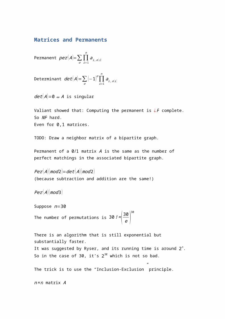
Matrices and Permanents

Permanent per (A )=∑σ∏i=1

n

ai , σ ( i)

Determinant det (A )=∑σ

(−1 )σ∏i=1

n

ai ,σ (i )

det (A )=0⇔A is singular

Valiant showed that: Computing the permanent is ¿P complete. So NP hard.Even for 0,1 matrices.

TODO: Draw a neighbor matrix of a bipartite graph.

Permanent of a 0 /1 matrix A is the same as the number of perfect matchings in the associated bipartite graph.

Per (A ) (mod 2 )=det (A ) (mod 2 )(because subtraction and addition are the same!)

Per (A ) (mod 3 )

Suppose n=30

The number of permutations is 30 !≈( 30e )30

There is an algorithm that is still exponential but substantially faster.It was suggested by Ryser, and its running time is around 2n. So in the case of 30, it’s 230 which is not so bad.

The trick is to use the “Inclusion-Exclusion” principle.

n×n matrix AS non-empty set of columns.

Ri (S ) – Sum of entries in row i and columns from S.

Per (A )=∑S

(−1 )n−|S|∏i=1

n

Ri (S )

Since we go over all S, we have 2n terms. The running time is something around 2n times some polynomial.

Per ( x11 … x1n⋮ ⋱ ⋮xn1 … xn

)=∑σ ∏ix i , σ (i )=¿

Multilinear polynomial. n!monomials. Each monomial is a product of variables. We have n2 variables.This applies both to the determinant and the permanent.

In Ryzer’s formula we only get monomials with n variables – 1 from each row.In the original definition we also get monomials with n variables – 1 from each row. But each of them must be from a different column.

First let’s see that all the terms that should be in Ryzer’s formula are actually there.

∏i=1

n

xi , σ ( i) - only for S=¿ all columns.

This is a monomial that includes 5 variables but only 3 columns:x11 x21 x33 x32 x55

n variables, c columns – {1,3,5 }c⊂S

The number of minus signs: ∑S∨c⊂S

(−1 )n−|S|∙1Term=0

TODO: Draw many partially drawn matrices.

For every variable independently, substitute a random value {0 ,…, p−1 } p>n2 , p is prime. Then compute the determinant.And we can even do the computations modulo p.

Lemma: For every multilinear polynomial in n2 variables, if one substitutes random values from 0 ,…, p−1 and computes modulo prime p, the answer is 0 with probability at most

n2

p.

ax+b=0 (mod p ) the probability is 1p

Suppose the probability is kp for k variables. We want to show it’s

k+1p for k+1 variables.

We can look at the new polynomial as p (x1 ,…, xk+1 ) xk+1 ( p1 (x1 ,…,xk )+ p2 (x1 ,…, xk ))

If p1 and p2 are zero, this happens in probability kp (by induction) and otherwise, there’s

only one possible vale of xk+1 such that everything is zero. So the total probability is (k+1 )p

Kastaleyn: Computing the number of matchings in planar graphs is in polynomial graphs.

Kirchoff: Matrix-tree theorem. Counts the number of spanning trees in a graph.

We have a graph Gand we want the number of spanning trees.

Laplacian of G – L.v1 … vnv1 d1 ¿

¿⋮ ¿0 ¿⋱¿¿vn ¿¿¿dn ¿

li , j=l j , i=−1 ∙ ( ⟨ i , j ⟩∈E )li ,i=¿ degree of vertex i

TODO: Draw the graph and its corresponding matrix(though we got the point)

The algorithm: Generate the Laplacian matrix of the graph. Cross some row and column (same column) and calculate the determinant. This is the number of spanning trees of the graph.

Given G, Direct its edges arbitrarily. Create the incidence matrix of the graph.

e1 e2 e3 e4v1 +1 0 ¿

0¿v2 ¿−1¿−1¿+1¿0¿ v3¿0¿0 ¿−1¿−1¿v4 ¿0¿+1¿0¿+1¿

For each edge you put a +1 for the vertex it is entering and −1 for the vertex it leaves.Denote this matrix M .

If we multiply M ∙M T we get the Laplacian.The incidence matrix has special properties. One of the properties is its “Totally Unimoduler”.Totally unimodular: Every square sub-matrix has determinant either +1 ,−1 or 0.

Theorem: Every matrix in which every column has at most a single +1, at most a single −1 and rest of the entries are zero, is totally unimodular.

--- end of lesson

Given a graph G we have its Laplacian denoted L.Also M is the vertex-edge incidence matrix.We know that MM T=LAnother thing we said about M is that it’s totally unimodular. Which means that every square submatrix has determinant either 0,1 or +1.

Wlog, we always look at the case where m≥n (m is the number of edges, n is the number of vertices).If the number of edges is smaller than the number of vertices, either we can use all edges as a spanning tree or we don’t have a spanning tree.

rank (M )≤n−1

Let’s observe the matrix transposed:TODO: Draw a transposed incidence matrix.

If we take x=[1 … 1 ]Then x∈ ker M

What do we know about a submatrix with a subset of the edges (but all the vertices)

If S is a spanning tree, then the rank is n−1.Otherwise, then rank<n−1

det (M s−i ∙ M s−iT )=det ( M s−i )∙ det (M s−i

T )=1 if S is a spanning tree and 0 otherwise.

Denote M s−i=M S'

So the number of spanning trees = ∑Sdet M S

' ∙ det M S'

Binet-Cauchy Formula for computing a determinant:Let A and B be two matrices. Say A is r ×n and B is r ×n, n>r.

Then det A ∙ BT=∑

S(det AS ) (det BS )

(S ranges over all subsets of r columns)

If r=n then det (A ∙ B )=(det A ) ∙ (det B )If r>n the determinant is zero. So it’s not interesting.If n>rSet A=B=M−i. Then everything comes out.

Prove the Binet-Cauchy formula:

Δn×n

¿=[x1 0 00 ⋱ 00 0 xn

]¿det (A ΔBT )=∑

S(det A ) ∙ (det BS ) ∙(∏i∈S

x i)We will prove this, and this is a stronger statement then the one we need to prove.

The answer A ΔBT is an r ×r matrix:Every entry in the matrix is a linear polynomial in the variable x i. Linear because we never multiply an x i in x j. In addition we don’t have any constant terms.

What is the determinant?

det (A ΔBT ) is a homogenous polynomial of degree r .

We can take any monomial of degree r , and see that the coefficients in both cases are the same.

On the right hand side we don’t have any monomials of degree higher than r or lower than r. We need to prove they are zero on the left side.T=¿ a set of less then r variables.

Substitute 0 for all variables which are not in T .

A Δ' BT

BAAAAHHH. Can’t write anything in this class!

Spectral Graph TheoryNP-Hard problems on random instances.

Like 3SAT , Hamiltonicity k-clique, etc…We sometimes want to look at max-clique (which is the optimization version of k-clique).We can also look at the optimization version of MAX-3SAT.

3XOR or 3LIN:

(x1⊕ x2⊕ x3 )…This problem is generally in p. But if we look for the maximal one we get an NP-Hard problem.

Motivations:- Average case (good news)- Develop algorithmic tools

- Cryptography- Properties of random objects

Heuristics:3SAT: “yes” – Find a satisfying assignment in many cases (yes/maybe).Refutation/”no” – find a “witness” that guarantees that the formula is not satisfyable. (no/maybe).

HamiltonicityGn , p - Esdes-Rengi random graph model:Between any two vertices independently, place an edge with probability p.G

n , p=5n. The p doesn’t have to be a constant.

Process of putting edges in the graph at random one by one.

3SAT: At first, a short list of clauses is satisfyable. But as the formula becomes larger, it is not so sure that it is satisfyable.What is that point?A conjecture is t 4.3 ∙ n.There is a proof of 3.5 ∙ n.However, there is a proof that this is a sharp transition.For refutation, the condition is exactly opposite. The longer the formula, the easier it is to find a witness for “no”.

--- end of lesson

Adjacency matrix:

[ 0 ¿1⋱ ¿ ¿0¿] a i , j=1⇔ (i , j )∈E

For regular graphs, there is no difference between the adjacency matrix and the laplacian. For irregular graphs, we do have differences and we will not get into it.

Properties: Non-negative, symmetric, connected ⇔ irreducibleIrreducible means we cannot represent it as a block matrix such that the upper right block is zeroes.

λ1≥ λ2≥…≥ λn are all real, we might have multiplicities so we also allow equality.v1 ,…,vn eigenvectors.

If we take two distinct eigenvalues λ i≠ λ j then vi⊥v j

Rn has an orthogonal basis using eigenvectors of A.

If we look at the eigenvector that corresponds to the largest eigenvalue, then the eigenvector is positive (all its elements are positive).

λ1> λ2 , λ1≥|λn|(The last 2 properties are only true if the graph is connected)

x is an eigenvector with eigenvalue λ if Ax=λx

In graphs, if we have the adjacency matrix, and we multiply it by x.The values of x corresponds to values we give to some of the vectices of A.

TODO: Draw graph.

If some x is an eigenvector of A, it means every vertex is given a value that is a multiple of the values of its neighbors.

traceA=0∑ λi=trac e

Since λ1>0⇒ λn<0

Bipartite GraphsLet x be an eigenvector with non-zero eigenvalue λ.

TODO: Draw bipartite graph

By flipping the value of x on one site of the bipartite graph, we get a new eigenvector and it has eigenvalue – λ.This is a property only of bipartite graphs (as long as we’re dealing with connected graphs).

Consider an eigenvector x. Then observe:

xT AxxT x

This is called Rayleigh quotientsIf x is an eigenvector of eigenvalue λ⇒xT λxxT x

=λ ∙ xT xxT x

=λ

Let v1 ,…,vn be an orthonormal eigenvector basis of Rn.In this case:x=a1 v1+…+an vn where a i=⟨ x , v i ⟩

A (∑ ai v i )=∑ ai λi v i

(∑ ai bi )T (∑ ai λi v i )=

∑ ai2 λi

∑ a i2

This is like a weighted average where every λ i gets the weight a i2

So this expression cannot be larger than λ1 and cannot be smaller than λn

Suppose we know that x⊥ v1?It means that the result is a weighted average of all vectors except for λ1

Another way of getting the same thing:

∑i , j

aij x1 x j (element-wise multiplication of the matrix A and the matrix x ∙ xT.

Large max cut ⇒ λn is close to −λ1Can show it using rayleigh’s quitients.But the interesting thing is that the opposite direction is not so true!

We looked at the relation between λ1 and λn. Now let’s look at the relation between λ1 and λ2.If a graph is d-regular all 1 eigenvalue.If we have a disconnected d-regular graph, λ1, λ2 are equal! Since 111111… is an eigenvector of both λ1 and λ2.So if they are equal, the graph is disconnected!

What happens if they are close to being equal?

λ2 close to λ1, then G close to being disconnected!

Suppose we have a graph. TODO: Draw the graph we are supposed to have.

We perform a random walk on a graph. What is the mixing time?If a token starts at a certain point, what is the probability it will be in any of the other vertices? If it turns quickly into a uniform distribution then the mixing is good.

Small cuts are obstacles of fast mixing.

If we started on the first vertex, we can say we started with the (probabilities) vector:[1 0 … 0 ]

A∑ ai v i

d

If I do t steps of the random walk it’s: At

d t (∑ ai v i )=∑ ai (λi )

t x i

d t

If λ i≫|λl| then we get a uniform distribution over all vertices.

λ1 for non-regular graphsSuppose the graph has maximum degree Δ and average degree d .So we know λ1≤ ΔBut this is always true: λ1≥d

xT= (1,1,…1 ) and consider xT AxxT x

So:

xT AxxT x

=¿ sum over all entries of A = 2mn

≥ average degree.

c-core of a graph is the largest subgraph in which every vertex has degree ≥c.

Let c¿ be the largest c for which the graph g has a c-core.

At d-regular graphs c¿=d.

λ1≤c¿

v is the eigenvector associated with λ1. Sort vertices by their value in the vector v.So v1 is the largest value and vn is the smallest. And all numbers are positive (according to the provinious bla bla theorem).

The graph cannot have a λ1+1-core.(a vertex cannot be connected to λ1 neighbors above it, since then it cannot equal to a multiple λ1 of the values of its neighbors)

If we look at a star graphΔ=n−1d=2 (a bit less than)And the largest eigenvalue λ1=√n−1We can give the center √n−1 and the rest 1.

Sometimes when we have a graph that is nearly regular but have a small number of vertices with a high degree, we should remove the vertices of high degree since they skew the spectrum!

Let’s use α (G ) to denote the size of the maximum independent set in the graph.And let’s assume that G is d-regular.

α (G )≤−nλn

d−λn

G is bipartite. Then λn=−λ1 and then α (G )=n λ12λ1

=n2

Proof: λn≤xT AxxT x

∀ x

Let S be the largest independent set in G.

TODO: Draw x

So the entries of s will equal n−s and the other vertices will be – s

¿

λ1≤s2 (nd−2ds )−2 s (n−s)ds

s (n−s )2+ (n−s) s2=s2nd−2d s3−2 s2nd+2d s3

s (n−s ) ( (n−s )+s )=

−sdn−s

λn ∙ n− λn s≤−dss (d− λn )≤−λnn

s≤− λnnd− λn

If |λn|≪d we get a very good bound. Otherwise we don’t.

∑ λi=0

We can also look at the trace of A2=∑ (λi )2

On the other hand, it is also ∑ d i

Only for regular graphs, this is n ∙dSo it follows that the average square value: Avg ( λi2 )=d

Avg|λi|≤√d

Recall that λ1=d!

It turns out that in random graphs (regular or nearly regular).

With high probability ∀ i≠1⇒|λi|=O (√d )

In almost all graphs, |λ1|≫|λn|

Therefore: s≤− λnnd− λn

≤ 2√d nd+2√d

≤ 2n√d